Page 1
International Journal of Computer Applications (0975 – 8887)
Volume 129 – No.2, November2015
45
Implementing Entropy Codec for H.264 Video Compression Standard
Mohamed Abd Ellatief Elsayed
Communication Department, Ain shams university
Abdelhalim Zekry Faculty of Engineering, Ain Shams University
ABSTRACT
Entropy coding is a lossless compression technique which is
supported in H.264/AVC standard by different techniques.
According to baseline and the extended profiles of
H.264/AVC, two variable length techniques are for seen. The
first one is context adaptive variable length coding (CAVLC)
and the other is exponential Golomb (Exp-Golomb) one. The
CAVLC is used to quantize transform residues after
reordering them by ZigZag scanning while Exp-Golomb
coding is used to quantize other syntax elements. Within the
frame of realizing the whole H246 standards, this paper,
introduces an implementation of these two codec techniques
for baseline profile using Matlab and Simulink. The main
concept is to implement CAVLC and Exp-Golomb decoder
according to H.264/AVC standard and then device
a technique to implement CAVLC & Exp-Golomb encoder.
The different implementations are utilized to verify each
other.
Keywords
Context adaptive variable length coder (CAVLC),
Entropy coding, Exp-Golomb, H.264/AVC.
1. INTRODUCTION H.264/ MPEG-4 AVC is a video codec standard that is
currently one of the most commonly used formats for the
recording, compression, and distribution of video content.
The standardization of the first version of H.264/AVC was
completed in May 2003. The functional block diagram of
H.264 encoder/decoder is shown in Fig.1.As shown in Fig.1,
entropy coding is the last block in encoder after the
transform quantization and the fist block in decoder before
the inverse quantization. H.264 supports two techniques for
entropy encoding. The first one is the Context adaptive
variable length coding (CAVLC) for the quantized transform
residues after ordering them by ZigZag scanning together
with Exponential Golomb coding, Exp-Golomb, for other
syntax elements. The other technique is to use Context
adaptive binary arithmetic coding (CABAC).CABAC has a
higher compression performance but unlike CAVLC, it is not
supported in all H.264 profile like baseline and extended
profiles [1].
H.264/ MPEG-4 AVC support Context adaptive variable
length coding (CAVLC) as one of entropy encoder methods
to achieve a higher compression ratio [2]. Compared with
previous variable length coding, CAVLC achieves better
coding efficiency. Because of its adaptive part that makes the
encoding of each block depend on the number of non zero
transform coefficient in the upper left part of the block. But
that makes the algorithm complexity higher. CAVLC
decoder is used in all the upcoming media applications that
have adopted H.264 video standard:
- Digital TV (satellite, cable, IPTV, over-the-air broadcast
etc).
- High-Definition Optical Discs (Blu-ray Disc, and
HDDVD).
-Real time Image Processing Applications(video
conferencing and video telephony).
-Portable device applications (cell phones and portable media
players).
Fig: 1 Typical H.264 Encoder/Decoder [1]
In this paper, an implementation of Entropy decoder of
Baseline profile is presented according to standard, which
means to implement Exponential Golomb and CAVLC in
Matlab and in Simulink and propose a method to implement
the Entropy encoder in Matlab and Simulink as the encoder
is not specified in the standard. In the next section the
exponential Golomb design and implementation will be
described in detail.
2. EXPONENTIAL GOLOMB
PRINCIPLES Exponential –Golomb codes are binary codes with variable
length constructed according to a regular pattern.Exp-
Golomb supported by H.264 standard for encoding almost all
syntax elements except those related to quantized transform
coefficients [3][4].Variable length codes such as Exp-
Golomb is considered an efficient way of representing syntax
elements by assigning short code words to frequently
occurring syntax elements and long code words to less
common syntax elements.[5].
Page 2
International Journal of Computer Applications (0975 – 8887)
Volume 129 – No.2, November2015
46
Table 1 shows the first few Exp-Golomb code words that
indexed by code Numbers. Also fromTable1 it is noticed that
these codes have a regular logical construction. So it can be
encoded and decoded logically without the need for look-up
table. An Exp Golomb codeword has the following structure:
[M Zeros Prefix] [1] [INFO] (0)
Table1. Exp-Golomb Code words
Bit string form Range of code Num
1 0
0 1 X0 1…2
0 0 1 X1 X0 3…6
0 0 0 1 X2 X1 X0 7…14
0 0 0 0 1 X3 X2 X1 X0 15…30
0 0 0 0 0 1 X4 X3 X2 X1 X0 31…62
…. ….
Each codeword has a prefix of M zeros followed by 1 which
is followed by INFO. Accordingly it is M-bit field carrying
information. The first codeword has no leading zero or
trailing INFO. Code words 1 and 2 have a single-bit INFO
field; code words 3–6 have a two-bit INFO field and so on.
The length of each Exp-Golomb codeword is (2M + 1) bits
and each codeword can be constructed by the encoder based
on its index code num as following:
M = floor (log2 [code Num + 1]) (1)
INFO = code Num + 1 − 2M (2)
A codeword can be decoded as follows:
1. Count number of zeros till reaches 1 this number is
M.
2. Read M-bit INFO field.
3. Code Num = 2M+ INFO – 1
Code Num can be derived from Syntax element by different
ways according to syntax element type as the standard
supports 4 syntax element types ( Unsigned(Ue) , Signed(Se)
, Mapping(Me) , Truncated (Te)). Mapping of syntax
element to code Num for each type shall be according to the
following procedure:
1-For Unsigned direct mapping, code num = syntax element.
Used for macro block type, reference frame index and others.
2- For Truncated mapping: if the largest possible value of
syntax element is 1, then a single bit b is sent where
b =! Code num, otherwise Ue mapping is used
3- Signed mapping, used for motion vector difference, delta
QP and others. Syntax element is mapped to code num as in
Table2.
Table2. Signed mapping
Code Num Syntax element value
0 0
1 1
2 -1
3 2
4 -2
5 3
6 -3
K (-1)K+1 Ceil(K+2)
4- Mapped symbols: syntax element is mapped to code num
according to a table specified in the standard [1][2].
2.1 Exponential Golomb Implementation
and Verification At first the Exponential – Golomb is implemented as an m-
file in Matlab. Fig 2 shows the flow chart of the exponential-
Golomb encoder implemented by Matlab. First step in
encoder is to define the type of the syntax element. If the
syntax element type is unsigned, then code Num equal
syntax element. If the syntax element type is signed, then
code Num calculates as in table2. If the type is mapping, one
uses certain tables defined in the standard to obtain Code
Num from syntax element. After calculating Code Num, one
calculates M and Info and uses them to obtain encoded bits.
Note that the truncated syntax element type encoded as
unsigned if syntax element has value more than 1.And if
syntax element equal 1 only one bit will be sent .When the
input is a syntax element from unsigned type with a value of
226 to the encoder, it outputs the following result:
Encoded bits = 000000011100011
This result can be confirmed by simple processing of the
input according to equations (0), (1), and (2):-
1-M=Floor [Log2 [226+1]] =Floor 7.826538. Then M=7
zeros.
2-INFO=226+1-27=99 then binary form of info =1100011.
3-I follow that the Encoded bits of 226 should be
000000011100011.
Fig 2: The flow chart for exponential Golomb encoder
Page 3
International Journal of Computer Applications (0975 – 8887)
Volume 129 – No.2, November2015
47
The decoder performs the inverse process of the encoder
where it restores the original data form of decoded one. Fig 3
shows the flow chart of Exponential Golomb decoder
implementation in Matlab. First step in decoder is to count
the number of leading zeros of the received encoded bits to
calculate M. Then calculate Info from the part after the first
one. Then one uses M and Info to calculate code Num. One
has to know the type of the received encoded bits to
determine how to calculate syntax element from it. Note that
the truncated syntax element type decoded as unsigned if
syntax element has value more than 1.And if syntax element
equal 1 only one bit will be received. When the input
encoded bits are “000000011100011” and the syntax type is
unsigned, the output will be a syntax element = 226. To
verify the correctness of the processing in the decoder the
data is calculated according to the steps:
1-Count zeros before the first 1, then M=7
2-INFO=1100011, which means in decimal INFO=99
3- Syntax element =2^7+99-1=226 which is the same
output value from the encoder.
Fig 3: The flow chart of Exponential –Golomb decoder
Fig 4: Simulink Exp-Golomb codec model
Fig 4 shows the Simulink model of the implemented Exp-
Golomb codec built according to the Matlab model
developed in the previous section. The encoder takes syntax
element and type, while in case of mapping type it also takes
chroma and prediction, as input. The first step in encoder is
to calculate Code Num then calculate M and Info then use
them to figure out Encoded bits. The decoder takes encoded
bits and type, while in case of mapping type it also takes
chroma and prediction, as input. The first step is to count
leading zeros to calculate M then uses it to calculate Info and
at last decodes Code Num then calculates syntax element
according to syntax type. The model consists of the encoder
and decoder in a loop back connection for the functional
verification of the whole codec. It is clear from the figure
that the error counter of the difference between the input and
the output is equal to zero proving the correctness of the
Simulink implementation
3. CAVLC PRINCIPLE In this section Matlab implementation of the CAVLC will be
carried out similar to Exp-Golomb codec. The Context
adaptive variable length coding (CAVLC) is an Entropy
coding method which is used to compress digital data by
examining the frequency of patterns within it and
representing frequently occurring patterns with smaller
number of bits. It is used to encode quantized residual data of
4X4 or 2X2 blocks of transform coefficients. A residual
block is the difference between the predicted and the input
video data and is obtained after integer discrete cosine
transform and quantization. In order to increase compression
ratio, CAVLC in h.264 standard introduces the concept of
context model to map the probability of symbols more
accurately. However, to provide such a high compression
ratio the computational complexity becomes higher because
of search for code words in several look-up tables. CAVLC
is designed to take advantage of several characteristics of
quantized 4x4 blocks of transform coefficients such as:
- Existence of long runs of zeros after zigzag scanning.
-Highest number of non-zero coefficients after zigzag
scanning are often sequences of +/-1.
-The number of non-zero coefficients in neighboring blocks
is correlated.
-Level of non-zero coefficients is usually higher at the start
of the reordered array near the DC coefficient, and lower
towards the higher frequencies.
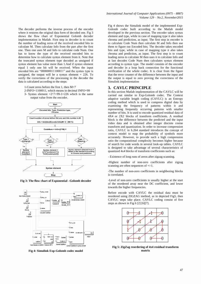
Before encode with CAVLC the residual data must be
reordered using ZIGZAG method, as in depicted Fig5, then
CAVLC steps take place. CAVLC coding consist of five
steps as shown in Fig 6 [2] [6][7].
Fig 5: ZigZag reordering of 4x4 residual transform
matrix
Page 4
International Journal of Computer Applications (0975 – 8887)
Volume 129 – No.2, November2015
48
Fig 6: CAVLC coding flow chart
1-Coeff_token: This step encodes the number of nonzero
coefficients (TNZ) and the number of trailing ones (T1).
TNZ can be anything from 0 to 16 and T1 can take values
from 0 to 3. If there are more than three trailing +/−1s, only
the last three are treated as „special cases‟ and any others are
coded as normal coefficients. There are four choices of look-
up table to use for encoding Coeff_token, three variable-
length code tables and a fixed-length code table. The choice
of table depends on the number of non-zero coefficients in
the left and upper previously coded blocks, nA and nB
respectively [8]
- If nA , nB >0 then nC=nA + nB >>1,
- Else if only nB=0 then nC=nA,
- Else if only nA=0 then nC=nB,
- Else nC=0
After calculating nC parameter, then choose one of look-up
tables for encoding according to Table3.
Table 3. Choice of look-up table for Coeff_token
nC Tables for Coeff_token
0,1 VLC table 1
2,3 VLC table 2
4,5,6,7 VLC table 3
8 or above FLC, fixed length coding
2- Sign of trailing ones: One bit to code the sign of each
trailing ones, 0 for positive sign, and 1 for negative sign.
3- Levels: In this step encode the sign and magnitude of the
remaining nonzero coefficients in reverse order level
composed of two parts, level_prefix and level_suffix.
Level_prefix is a b leading zeros followed by 1 according to
Table4.
Table4. Codeword table for level_prefix
level_prefix bit string
0 1
1 01
2 001
3 0001
4 00001
5 000001
6 0000001
7 00000001
…. …..
Level_suffix is an integer code of size suffix length. Large-
magnitude coefficients have low probability, so, its suffix
length is large. Small-magnitude coefficients have high
probability, so, its suffix length is small. The choice of suffix
Length I subjected to the following rules:
Initial suffix Length = 0, except if ((TNZ>10) and (T1<3))
then initial suffix length =1.
If the magnitude of this coefficient is larger than a threshold,
increment suffix Length, up to a maximum suffix Length = 6
according to table5.
4- Total zeros: the sum of all zeros before each non zero
coefficient it coded according to look up table given by the
standards.
5- Run before: the number of run zeros preceding each
nonzero level in reverse zigzag order.
Table5. Thresholds for determining whether to increment
suffix_length
Current suffix
length
Threshold to increment suffix
length
0 0
1 3
2 6
3 12
4 24
5 48
6 highest value reached
3.1 Matlab CAVLC Encoder/Decoder
Implementation At first the Context adaptive variable length (CAVLC) is
implemented as m-file in Matlab. Fig 7 shows the flow chart
of CAVLC encoder. The Encoder takes syntax elements, nA
and nC as inputs. The first step is to reorder syntax elements
by ZigZag method. Then count the number of trailing ones
and determine the sign of each trailing ones. Then the
encoder calculates nC to define the look up table which is
used to obtain the Coeff_token according to the number of
trailing ones and total number of non zero coefficients
(TNZ). The next step is for- loop repeated by TNZ-trailing
ones to calculate level_prefix and level_suffix for every non
zero coefficient in order to calculate level_code. Finally, it
encodes the number of total zeros and each run of zeros
before each non zero element.
Page 5
International Journal of Computer Applications (0975 – 8887)
Volume 129 – No.2, November2015
49
Fig 7: The flow chart for CAVLC encoder
The decoder performs the inverse processes of the decoder,
where it restores the original form of the data. Fig 8 shows
the flow chart of Context adaptive variable length (CAVLC)
decoder implementation in Matlab. The Decoder takes
encoded bits, nA and nC as inputs. The first step is to
calculate nC to determine which look up table will be used in
calculating Total number of coefficient and number of
trailing ones. After that, the decoder calculates the sign of
each trailing ones according to that 0 means positive sign and
1 means negative sign. The next step is to decode Level and
sign for each total non zero coefficient. Then decode of the
total number of zeros and each run of zeros before every
TNZ. The last step is to reorder the data into 4X4 block
Fig 8: The flow chart for CAVLC decoder
3.1.1 Encoder Implementation Table6. CAVLC encoder example
Element Value Code
Coeff_token Total_Coeff = 5, T1s
= 3 (use Num VLC0)
0000100
T1 sign (4) + 0
T1 sign (3) - 1
T1 sign (2) - 1
Level (1) +1 (level prefix = 1 at
suffix Length = 0)
1
Level (0) +3 (level prefix = 001
at suffix length = 1)
0010
Total Zeros 3 111
run before(4) Zeros Left = 3; run
before =1
10
run before(3) Zeros Left = 2; run
before =0
1
run before(2) Zeros Left = 2; run
before =0
1
run before(1) Zeros Left = 2; run
before =1
01
run before(0) Zeros Left = 1; run
before = 1
No code required;
last coefficient.
The output
code word
000010001110010111101101
Here the encoding process will be demonstrated by an
example. The data to be encoded is given in fig 5 where it is
reordered by zigzag scanning resulting in the data series in
the form of (0, 3 , 0,1,-1, -1,0,1, 0, 0, 0, 0, 0, 0, 0, 0). The
encoding process is carried out according to the algorithm
given previously in fig 7. According to the first step in the
algorithm, the Total_coeff =5, T1=3 and nC is taken zero as
there is no previous encoded blocks. So, from table 3 these
values result in choosing (VLC table1).Two approaches are
used to obtain the VLC of Total_coeff and T1.
The first approach is to use the same order of the standard as
in Table 7 and calculate the required row number by this
equation:
If (Total_coeff >2) then row number=4(Total_coeff-3)
+T1+7,
Else if (Total_coeff ==2), then row number =T1+4,
Else if (Total_coeff ==1), then row number= T1+2,
Else row number =1
Table7: Coeff_token mapping to Total_coeff and trailing
ones
Row number T1 Total_Coeff 0≤ nC<2
1 0 0 1
2 0 1 000101
3 1 1 01
4 0 2 00000111
5 1 2 000100
6 2 2 001
7 0 3 000000111
8 1 3 00000110
9 2 3 0000101
10 3 3 00011
… … … …
Page 6
International Journal of Computer Applications (0975 – 8887)
Volume 129 – No.2, November2015
50
The second approach is to reorder the table of the standard to
make 2D table with 16 rows representing the Total_coeff and
4 columns representing T1 as shown in table 8.
Table8: Method to reorder Coeff_token mapping to
Total_coeff and trialing ones table.
Tota
l_co
eff
T1
0 1 2 3
0 1 ___ ___ ___
1 000101 01 ___ ___
2 00000111 000100 001
3 00000011
1
00000110 0000101 00011
… … … … …
1
5
00000000
00000111
00000000
00001010
00000000
00001001
00000000
00001100
1
6
00000000
00000100
00000000
00000110
00000000
00000101
00000000
00001000
The second Step in the encoding process applied on the
example: here there are three trailing ones with sign +,-,- so
the encoded symbol will be 011 as given in Table 6.
The third Step in the encoding process: this step encodes the
remaining non zero coefficients +3 and +1. Each coefficient
is transformed to level code by transforming positive
coefficient to even level code and negative coefficient to odd
level code according to the following rules:-
Levelcode = 2*Coefficient -2 for positive coefficient,
Levelcode = -2*Coefficient -2 for negative coefficient,
If ((index of coefficient == number of trailing ones) &
(number of trailing ones <3) then,
Levelcode = Levelcode -2
Then each level code encoded has two parts, a level_prefix
which is determined as in table 4 and a level_suffix which is
determined according to the following rules:
Initial suffix_length is calculated as in section 4 and
incremented as in table 5.
If (level_code binary right shifted by suffix_length) <14,
Then level_prefix= (level_code binary right shifted by
suffix_length),
And Levelsuffixsize =suffix_length,
Else if ((level code<30) & (suffix_length==0)),
Then level_prefix=14 and Levelsuffixsize=4,
Else if ((suffix_length>0) & (level_code binary right shifted
by suffix_length==14),
Then level_prefix=14 and Levelsuffixsize= suffix_length,
Else level_prefix=15 and Levelsuffixsize = 12 (as in baseline
profile level_prefix maximum value is 15).
Let us apply the above rules in this example. The first non
zero coefficient is +1.The level code for that coefficient =0
and the initial suffix_length=0. So level_prefix is equal 1
from table 4 and Level_suffixsize =0.Then the codeword for
+1 will be 1. Similarly, the codeword of +3 is 0010 as in
table 6.
The fourth Step for encoding in this example: the total non
zero elements is equal 5 and the total zeros before these
elements is equal 3. From the look up table in the standards,
the code word will be „111‟.
The fifth Step for encoding: in this step the encoder encodes
the number of zeros before each non zero element. In table 6,
the number of non zero elements equals 5, so as shown for
each element, there is a code word except for the last one as
the total zeros are encoded before .This code word is
calculated from a the look up table in the standard . For each
code word, the number of zeros before the non zero
coefficient and the number of zeros left are needed. For
example the first non zero coefficient has 1 zero run before
and the zeros left =3 so from the look up table its code word
is 10 and so on for the remaining run before.
3.1.2 Decoder Implementation Decoder must restore the original data from the encoded data
according to flow chart in fig 8. As has been done with the
encoder, the decoder will be implemented in this section on
the light of an example, where the above encoded sequence
will be the input to the decoder and transformed back to its
original form so the input to the decoder is
000010001110010111101101.
Table 9: CAVLC Decoder example
Code Element Value Output
array
0000100 Coeff_token TotalCoeffs = 5, T1s =
3
Empty
0 T1 sign + 1
1 T1 sign − −1, 1
1 T1 sign − −1, −1,
1
1 Level +1(suffix_Length=0;
increment
suffix_Length)
1, −1,
−1, 1
0010 Level +3 (suffix_Length =
1) 3, 1, −1,
−1, 1
111 Total Zeros 3 3, 1, −1,
−1, 1
10 run before 1 3, 1, −1,
−1, 0, 1
1 run before 0 3, 1, −1,
−1, 0, 1
1 run before 0 3, 1, −1,
−1, 0, 1
01 run before 1 3, 0, 1,
−1, −1,
0, 1
First Step: As shown in Table 9 first the decoder decodes
the TotalCoeffs and T1. This process takes long time, as in
the standard, for the VLC table with 4X4 block there are 62
Page 7
International Journal of Computer Applications (0975 – 8887)
Volume 129 – No.2, November2015
51
elements in the lookup table to be scanned to figure out the
TotalCoeffs and T1.So, it is tried here to subdivide this large
look up table into smaller ones according to the number of
leading zeros as shown in fig 9. Then one has to count the
number of leading zeros of the received stream and choose
the appropriate sub lookup table for it this will reduce the
number of access times of the lookup tables .Here using the
62 element look up table needs 18 access trials to find a
match. While with the use of these smaller look up tables the
access trial will be 3 times. The code word 0000100 means
that the total non zero coefficient =5 and the number of
trailing ones =3.
The second Step: from previous step the number of trailing
ones is 3 so the decoder takes the next 3 bits to determine
their signs.
62 E
lem
ent
look u
p t
able
1
Divide
into smaller look
up tables
000101 000101 000100 01 00011 00000111 000100 0000101 …. 000011 000000000000110 0000100 0000000000000101 0000000000001000 And So
on
Fig9: The large look up table for the Coeff_token is
divided into sub lookup tables according to the number of
leading zeros
Third Step: from step one the number of non zero
coefficients and the number of trailing ones are known.
Then, the difference specifies the number of times to repeat
this step to obtain the value and the sign of the remaining
non zero coefficient. Here the decoder count the no of zeros
to the known level_prefix then Levelsuffixsize is determined
according to the following conditions:
If( (level_prefix==14)&(suffix_length==0)
Then Levelsuffixsize =4,
Else if (level_prefix==15),
Then Levelsuffixsize=12
Else Levelsuffixsize = suffix_length.
After that the decoder converts the levelcode to the non zero
coefficient by the following rules:
Coefficient = (levelcode+2)>>1 for even levelcode.
Coefficient = (-levelcode-1)>>1 for odd levelcode.
As shown in table 9 (the Total non zero coefficient – the
trailing ones =2) so There are two non zero coefficient to be
decoded. The codeword of the first coefficient is „1‟ and
from table 4 it has level_prefix=0 and it has no level_suffix,
then the decoded levelcode = 0 and the decoded coefficient
=+1.By using the above rules once again, the codeword of
the second coefficient ‟0010‟ is decoded as +3.
The fourth Step in decoding: from step one, the total number
of non zero coefficients(TNZ) is 5, which means have to
search in column number 5 in the look up table proposed by
the standard to decode the total number of zeros. Here in this
example the required code word „111‟ and that means total
zeros before non zero elements equal 3 as in table 9.
The fifth Step in the decoding: from step one TNZ =5, so the
decoder has to decode the run before zeros to each
coefficient. There is a look up table in the standard defining
the code word of the run before zeros according to number of
zeros left and number of run before zeros. In this example, at
first the decoder put zero left = total number of zero which
decoded in step number four then zeros left =3.This means
that searching for a match from column number 3 in the look
up table. Here the decoder find a match for code word ‟10‟
which means that before element number five there is one
zero. By the same procedure ‟1‟, ‟1‟ ,‟01‟ means, before
element number four there is no zeros, and before element
number three there is no zeros ,while before element number
two there is one zero. The run before zeros before the
element number one did not have to be encoded because the
number of zero left is known from total zero which here is
one.
3.2 Cavlc Encoder/ Decoder Simulink
Implementation Fig 10 shows the Simulink model of the implemented
CAVLC encoder. The encoder takes Syntax element 4X4
blocks, nA and nB as inputs and run all steps as has been
done in the Matlab implementation. So, the first process in
the encoder is to reorder the input syntax by ZigZag method
then the first, second, fourth and fifth steps take place at the
same time as all these steps not depend on each other. The
third step and the final stage are enabled by the stage of step
1 and 2 block. To encode the remaining non zero coefficients
and after some delay, the first step enables the final stage
which reorder all the outputs from each stage and output the
encoded bits which represent the encoded syntax.
Fig 10: Simulink CAVLC encoder model
Fig 11 shows the Simulink model of the implemented
CAVLC decoder where the processing is carried out in
stages similar to the Matlab decoder model. The decoder
takes encoded bits, nA and nB as inputs. First step in decoder
is to decode token coefficient to calculate TNZ and trailing
ones. Two stages can proceed at the same time, namely the
second and third stage. The second stage is to figure out the
sign of each trailing ones. The third stage is to decode the
level and sign of each non zero coefficient and store these
levels in registers. Then, the fourth stage can proceed to
Page 8
International Journal of Computer Applications (0975 – 8887)
Volume 129 – No.2, November2015
52
decode the total number of zeros. Finally, stage five collect
all outputs from the previous stages and from registers and
decode run before zeros and then reorder all outputs in 4X4
block
Fig 12 shows the encoder and decoder of CAVLC in a loop
back connection for the functional verification of the whole
codec. It is clear from the figure that the error counter of the
difference between the input and the output is equal to zero
proving the correctness of the Simulink implementation.
Fig 11: Simulink CAVLC decoder model
Fig 12: CAVLC codec loop back for verification
Similarly, the CAVLC encoder, decoder and loopback
verification for 2X2 residual blocks are implemented
depicted in Figs 13, 14 and 15, respectively.
Fig 13: CAVLC 2X2 Simulink encoder
Fig 14: CAVLC 2X2 Simulink decoder
Fig 15: CAVLC 2X2 codec loopback for verification
4. CONCLUSION In this paper the implementation of encoders and decoders of
the Exponential Golomb and the CAVLC codec techniques
are carried out according to the standards of the video codec
H264 by Matlab and Simulink. This implementation is a
primary step towards VHDL implementation on FPGA. The
theoretical basis for the implementation is first described and
then appropriate algorithms of the codec are presented.
Matlab m-files are produced for all the encoders and
decoders. Then Simulink model is built for both codec. The
validation of the implementation is verified by straight
forward calculations and also by loopback method. This
project is a part of custom implementation of H264 video
codec.
Future work is to develop a technique to reduce the time of
searching tables in the decoder to reduce the time taken by
the decoder to decode a symbol. Implement encoder and
decoder of Exponential Golomb and CAVLC using VHDL
on FPGA.
5. ACKNOWLEDGEMENT The article is partially supported by a grant of the Foundation
of Computer Science, NY, USA vide FCS/RT56/15”
6. REFERENCES [1] ITU-T Recommendation H.264, 06-2011.
[2] Iain E.RICHARDSON, The H.264 Advanced Video
Compression Standard, Second edition , 2010, John
Wiley & Sons.
[3] Jorn Ostermann, Jan Bormans, Peter List,Detlev Marpe,
Matthias Narroschke, Fernando Pereira, Thomas
Stockhammer, and Thomas Wedi,”Video coding with
H.264/AVC:Tools, Performance, and Complexity”,
FIRST QUARTER 2004, IEEE CIRCUITS AND
SYSTEMS MAGAZINE
Page 9
International Journal of Computer Applications (0975 – 8887)
Volume 129 – No.2, November2015
53
[4] Detlev Marpe and Thomas Wiegand, Heinrich Hertz
Institute (HHI),Gary J. Sullivan, Microsoft
Corporation,” The H.264/MPEG4 Advanced Video
Coding Standard and its Applications”, August 2006,
IEEE Communications Magazine
[5] Iain E. Rechardson, "H.264 and MPEG-4 Video
Compression", 2003, John Wiley & Sons.
[6] ThomasWiegand, Gary J. Sullivan, Senior Member,
IEEE, Gisle Bjøntegaard, and Ajay Luthra, Senior
Member, IEEE, “Overview of the H.264/AVC Video
Coding Standard”, IEEE TRANSACTIONS ON
CIRCUITS AND SYSTEMS FOR VIDEO
TECHNOLOGY, VOL. 13, NO. 7, JULY 2003
[7] Xiaohua Tian, Thinh M. Le, Yong Lian, Entropy
Coders of the H.264/AVC Standard
[8] Algorithms and VLSI Architectures, 2011, SpringerA
HIGH PERFORMANCE AND LOW POWER
HARDWARE ARCHITECTURE FOR H.264 CAVLC
ALGORITHM, Esra Sahin and Ilker Hamzaoglu
Faculty of Engineering and Natural Sciences, Sabanci
University 34956, Orhanli, Tuzla, Istanbul, TURKEY.
IJCATM : www.ijcaonline.org