Portland State University Portland State University PDXScholar PDXScholar Dissertations and Theses Dissertations and Theses Spring 6-10-2014 Implications of Local and Regional Food Systems: Implications of Local and Regional Food Systems: Toward a New Food Economy in Portland, Oregon Toward a New Food Economy in Portland, Oregon Michael Mercer Mertens Portland State University Follow this and additional works at: https://pdxscholar.library.pdx.edu/open_access_etds Part of the Agricultural and Resource Economics Commons, Regional Economics Commons, and the Urban Studies and Planning Commons Let us know how access to this document benefits you. Recommended Citation Recommended Citation Mertens, Michael Mercer, "Implications of Local and Regional Food Systems: Toward a New Food Economy in Portland, Oregon" (2014). Dissertations and Theses. Paper 1892. https://doi.org/10.15760/etd.1891 This Dissertation is brought to you for free and open access. It has been accepted for inclusion in Dissertations and Theses by an authorized administrator of PDXScholar. Please contact us if we can make this document more accessible: [email protected].
Transcript
Portland State University Portland State University
PDXScholar PDXScholar
Dissertations and Theses Dissertations and Theses
Spring 6-10-2014
Implications of Local and Regional Food Systems: Implications of Local and Regional Food Systems:
Toward a New Food Economy in Portland, Oregon Toward a New Food Economy in Portland, Oregon
Michael Mercer Mertens Portland State University
Follow this and additional works at: https://pdxscholar.library.pdx.edu/open_access_etds
Part of the Agricultural and Resource Economics Commons, Regional Economics Commons, and the
Urban Studies and Planning Commons
Let us know how access to this document benefits you.
Recommended Citation Recommended Citation Mertens, Michael Mercer, "Implications of Local and Regional Food Systems: Toward a New Food Economy in Portland, Oregon" (2014). Dissertations and Theses. Paper 1892. https://doi.org/10.15760/etd.1891
This Dissertation is brought to you for free and open access. It has been accepted for inclusion in Dissertations and Theses by an authorized administrator of PDXScholar. Please contact us if we can make this document more accessible: [email protected].
D.2: CORRELATION BETWEEN PARCEL SIZE AND DISTANCE TO THE URBAN CORE ..........201
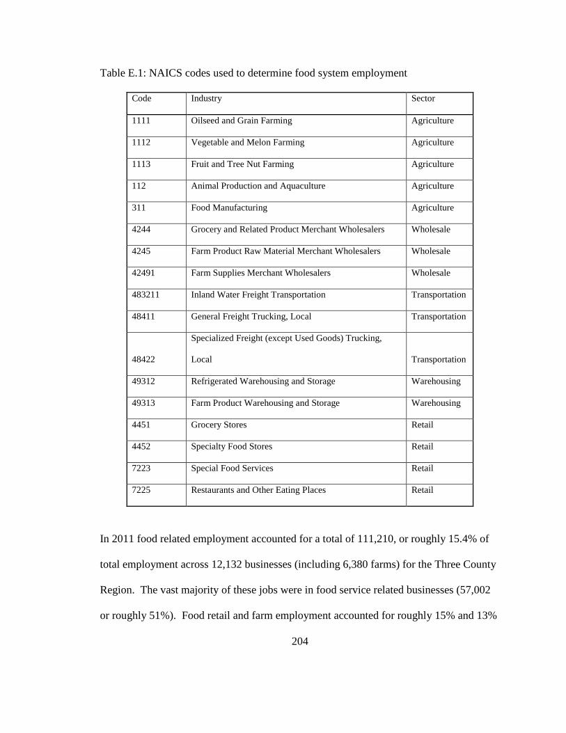
APPENDIX E: EMPLOYMENT IN FOOD RELATED ESTABLISHMEN TS IN
THE THREE COUNTY REGION...............................................................................203
APPENDIX F: AGRICULTURAL PRODUCER CHARACTERISTICS I N
CLACKAMAS COUNTY .............................................................................................207
F.1: FOOD GROWERS AND NON-FOOD GROWERS ............................................................208
ix
LIST OF TABLES
Table 1.1 Differences between global and local supply chains, actors and products
16
Table 2.1 Top retail establishments sales 2004-2012 ($1,000) 36
Table 3.1 Parameter estimates for predictors of proportion of small farms 72
Table 3.2 Number of farms by size class 79
Table 3.3 Acres by farm size class 79
Table 3.4 Farm value by value class 80
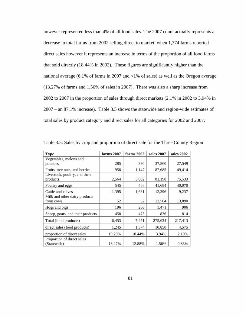
Table 3.5 Sales by crop and proportion of direct sale for the Three County Region.
81
Table 3.6 NAICS codes used to determine food system employment 86
Table 3.7 Regional food system employment by sector 87
Table 4.1 Methods for testing research hypotheses 88
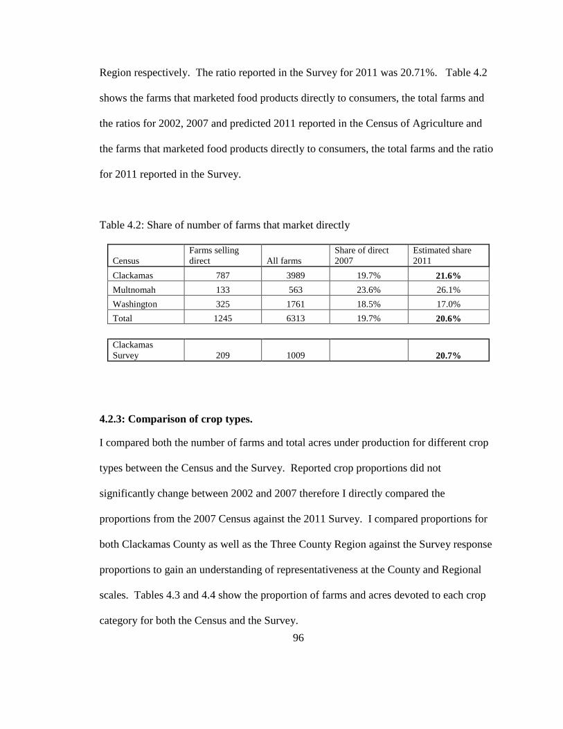
Table 4.2 Share of number of farms that market directly 96
Table 4.3 Proportion of farms of different crop types under production (Census v. Survey comparison)
97
Table 4.4 Proportion of acres of different crop types under production (Census v. Survey comparison)
97
Table 5.1 Sample size for spatial variables considered 111
Table 5.2 Moran’s I at different distance thresholds for Stage I analysis 120
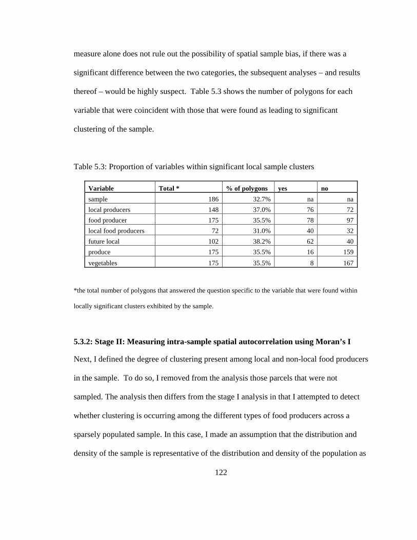
Table 5.3 Proportion of variables within significant local sample clusters 122
Table 5.4 Spatial autocorrelation of food producers at different distance thresholds
124
Table 5.5 Clustering differences of local and non-local food producers at different distance thresholds
128
x
Table 5.6 Impedance values assigned to road types 134
Table 5.7 Urban core neighborhoods 135
Table 6.1 Interviewee characteristics 147
Table 6.2 Parameter estimates for the relationship between off farm employment and urbanization
155
Table 6.3 Agglomeration externalities realized by different producer types 157
xi
LIST OF FIGURES
Figure 1.1 Conceptual model of the food system 11
Figure 1.2 Map of Portland Metro Area and the Three County Region 21
Figure 1.3 Map of Clackamas County Agricultural and Food Production Lands
24
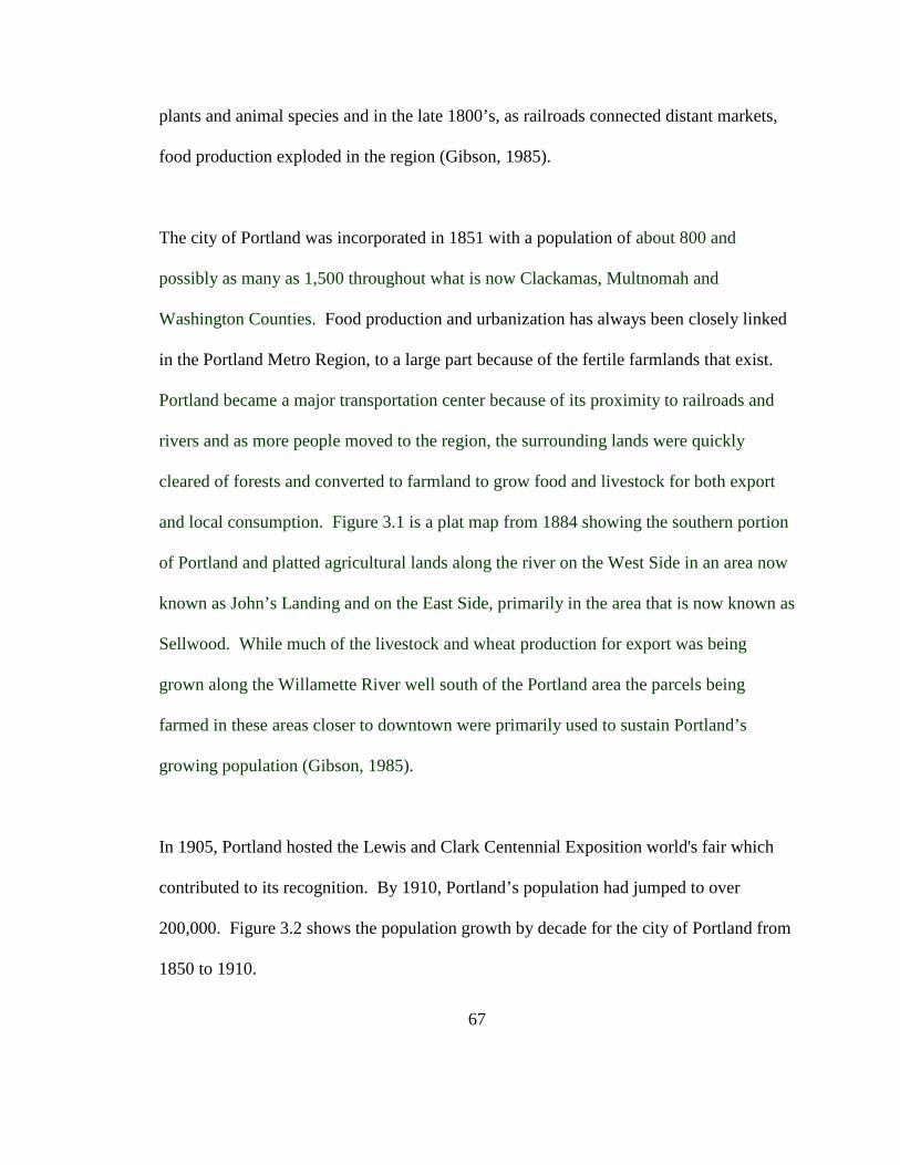
Figure 3.1 1884 plat map showing Downtown Portland and close in agricultural lands
68
Figure 3.2 Portland population growth, 1850 to 1910 68
Figure 3.3 Yamhill Street Market (circa 1919) 73
Figure 3.4 Portland Public Market (circa 1933) 75
Figure 4.1 Graphical representation of the four phase approach 87
Figure 4.2 2002, 2007 and predicted 2007 census age distribution 93
Figure 4.3 2002, 2007 and predicted 2011 census age distribution 94
Figure 4.4 Proportional age class comparison between the 2011 predicted Census of Agriculture and Survey respondents
95
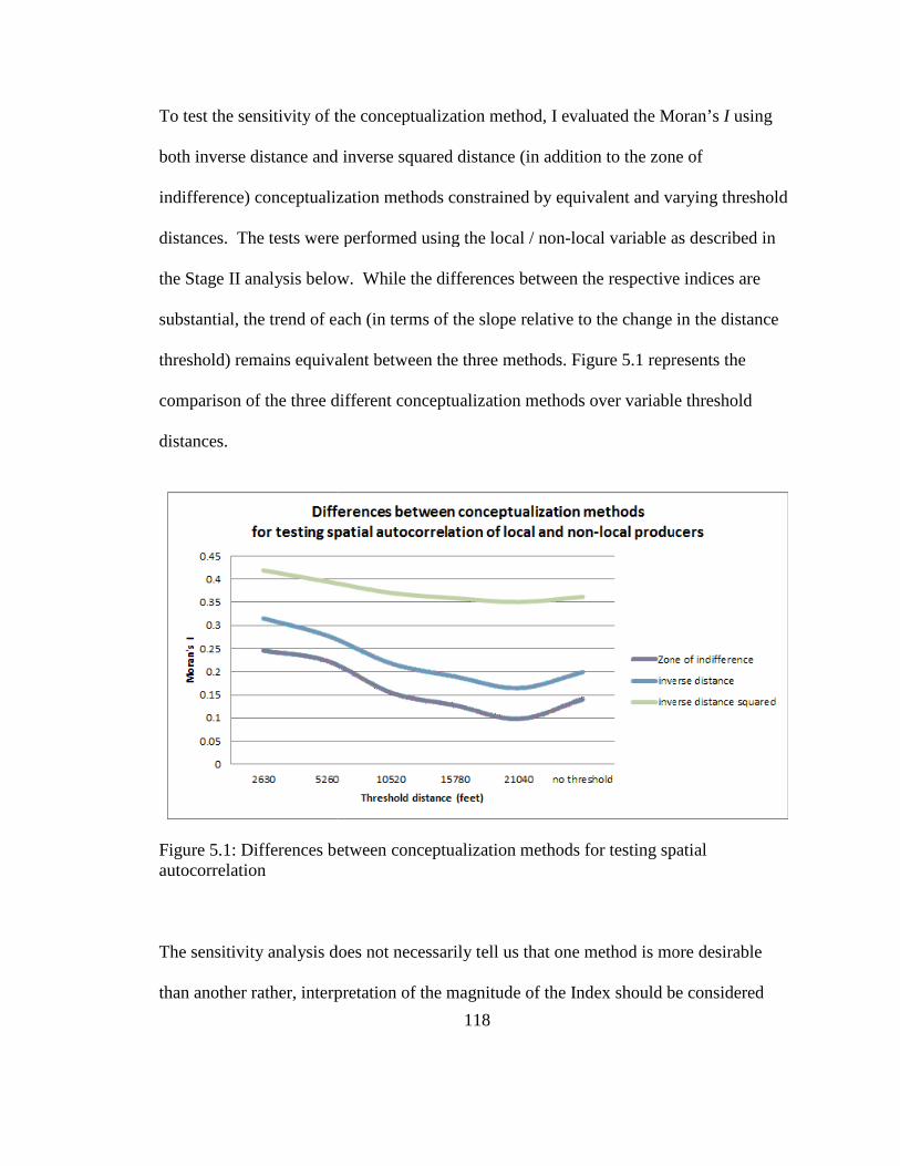
Figure 5.1 Differences between conceptualization methods for testing spatial autocorrelation
118
Figure 5.2 Map of locally significant clusters within the spatial sample 121
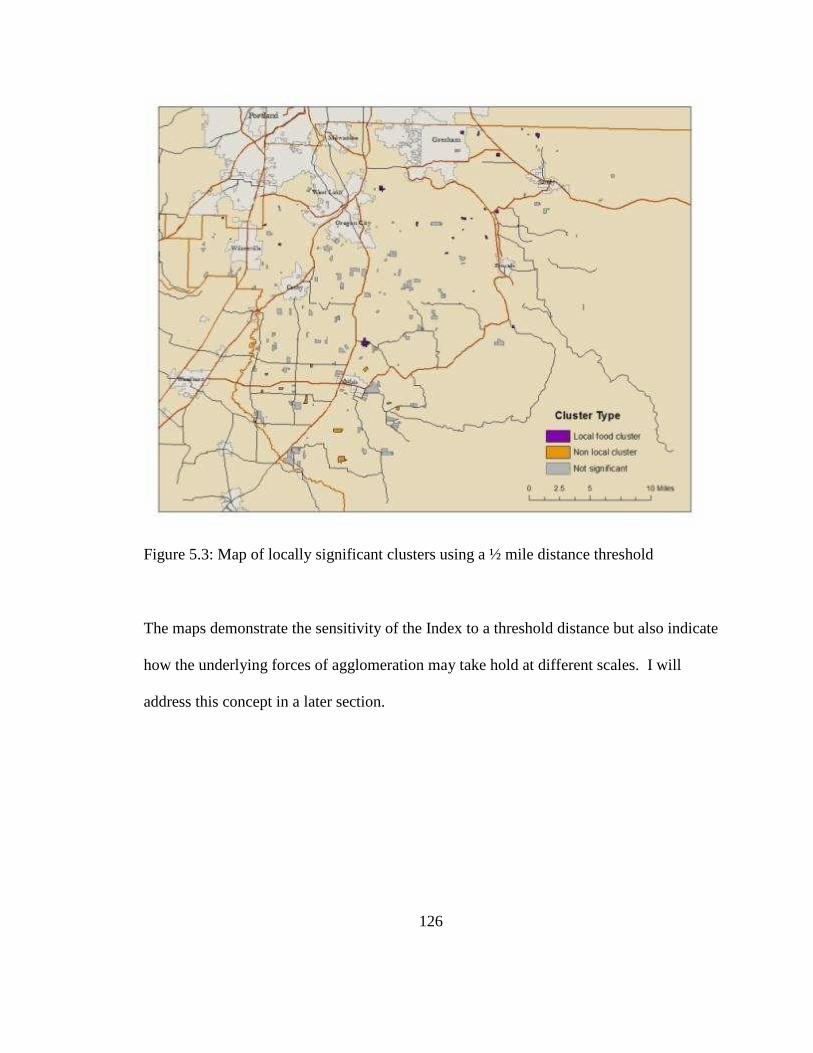
Figure 5.3 Map of locally significant clusters using a ½ mile distance threshold
126
Figure 5.4 Map of locally significant clusters using a three mile distance threshold
127
Figure 5.5 Influence of sample size on the stability of distance thresholds 131
Figure 5.6 Map of travel times to the urban core 136
Figure 6.1 Causes of agglomeration 144
1
CHAPTER I: INTRODUCTION
1.1: OVERVIEW
There has been a recent explosion of interest in the concept of local and regional food
systems as an alternative to the globalized agro-food sector both here in the Pacific
Northwest as well as throughout North America and Europe. Evidence of this emerging
popularity of more local forms of food production and consumption can be seen by both
the increase in alternative outlets such as farmers markets, CSAs and restaurants touting
local ingredients as well as institutional support such as farm to school programs and
other public sector procurement policies. So too has there been an explosion in research
pertaining to alternative food structures because, to a large degree, the many problems
associated with the industrialization of food chains are becoming apparent (Watts et al.
2005).
This recent rise in the prevalence of local and regional foods has been presented by many
as a means to resist the globalized agro-food structures (Hendrickson et al. 2001;
Hendrickson and Heffernan 2002; Allen et al. 2003; Hinrichs 2003; Selfa and Qazi
2005). Primary themes highlighted in the literature of alternative food systems include
embeddedness, authenticity, quality and shortened supply chains. Localization therefore
has been a natural extension of these themes in that “local” represents spaces for
resistance to the global system (Hendrickson and Heffernan 2002). And while the social
and environmental benefits are not explicit outcomes of localizing food supply chains,
the concept of localization often is seen as a panacea for all of the consequences of the
2
globalized system (Morris, Buller 2003). In addition, as an alternative to the social and
environmental failures of the globalized system, some scholars attest localized food
systems offer economic development opportunities that can be attributed to defensive
localism and import substitution (Bellows and Hamm 2001; Winter 2003; Swenson
2009). Yet, while the idea of local foods as an economic driver is clearly capturing the
imagination of a wide range of actors, much of the activity surrounding the issue exists at
the level of advocacy rather than in relation to empirical research that evaluates the extent
and impact of the sector on regional economies (Morris, Buller 2003).
In a 2013 special edition of “Journal of Agriculture, Food Systems, and Community
Development” that focused on research priorities, Boys and Hughes identify the need for
a better understanding of the regional economic benefits resulting from local food
systems particularly in terms of inter-firm networks that are formed through
agglomeration, firm clustering, and ultimately regional competitiveness and a means of
benefit generation through backward and forward supply-chain linkages. Highlighting
these research priorities, the authors point out that to date, little research or evidence has
been produced that draw from these analytical frames to support the thesis that local and
regional food systems actually do offer an opportunity for economic development. The
lack of evidence about the existing structures within the local and regional food sector in
terms of their impact on regional economies is a primary motivation behind the research
presented here.
3
The research pertaining to economic development opportunities associated with localized
food systems that does exist stems primarily from the rural development / re-structuring
paradigm. For example Marsden et al., (1999), Ross et al. (1999), Marsden et al. (2000),
Hinrichs (2003), Winter (2003), and Ikerd (2005) have all suggested that expansion of
local foods may be a development strategy for rural areas, particularly those areas that
have experienced negative effects of globalization. And while many scholars have
highlighted the importance of local food systems to regional economies (Feenstra 1997;
Trobe 2001; Renting et al. 2003; Star et al. 2003; Bhatia and Jones 2011), few have
sought to exploit recent theoretical frames advanced by researchers from the fields of
economic geography and regional science; the fields most concerned with regional
economic development. The concept of local and regional foods as a regional
development strategy and, by extension, the analysis of regional food systems in the
context of the city-region, present a unique theoretical lens of which new insights into the
factors that influence the emergence of such systems can be examined. Disciplines that
evaluate the influence of location and distance on economic activity are uniquely suited
to assess local food systems and the policies that affect them (Boys and Hughes 2013).
When contextualized at the regional scale, economic development takes on a different
meaning. Here, aspects of agglomeration economies become important in terms of the
clusters of economic activities that exist, and the diversity of industries within the region.
The research presented here draws from the disciplines of Economic Geography and
Regional Science to explore how knowledge accumulation and innovation diffusion
4
affect local and regional food system actors in terms of aspects of economic
development. I do so as an extension of, not an alternative to, the social theory and rural
development constructs outlined above. That is, the themes of embeddedness,
authenticity, quality and nature when coupled with and emerging from innovative city-
regions enable the emergence of the new food economy at the regional scale. In this
sense I have situated my analysis in terms of the city-region economy, and investigated
how a regional food system, including all of its components, distinct from that of the
export oriented, agro-food industry, might contribute to that economy.
Throughout this dissertation, I use the term “the new food economy”1 rather than terms
such as community food systems, sustainable agriculture, or alternative food networks as
often cited in the literature. The “new food economy” conjures aspects of economic
development that are not implicit in these other expressions and hence frames the
epistemological approach I have applied in my analysis. That is, I use the regional
economy as my unit of analysis, and while I do address other aspects of local and
regional food systems such as food justice, quality and embeddedness, resistance to
existing global food structures and commodity chains, concerns of environmental
degradation and health implications, my primary focus is on aspects pertaining to
regional economic development. Given this narrow scope, the work presented here
contributes evidence upon which additional research can be built so that economic
1 The “new food economy” was first coined by Winter (2001) and expanded upon by Blay-Palmer and Donald (2006) in their attempt to situate alternative food systems from a city-region and innovations perspective.
5
development professionals, urban and regional planners and concerned stakeholders can
make informed decisions specific to fostering these new food economies. Specifically,
the research presented here addresses the following research questions:
Research Questions:
• How does the new food economy differ from the traditional, globalized agro-food
industry?
• What are the implications of geographic space on how the new food economy
emerges?
• What are the implications for regional economic development stemming from the
new food economy?
In the following chapters I explore these questions through descriptive, qualitative and
quantitative analyses, focusing on a key set of hypotheses grounded in the literature.
Specifically I test three distinct hypotheses that together represent a dissertation of the
research questions. These hypotheses are as follows:
Hypothesis 1: Local and regional food systems in the Portland region and other regions
around North America and Europe can be differentiated from the export-oriented, global
agro-food sector;
Hypothesis 1b: As a sector, local and regional food systems are indeed new
relative to the export-oriented agro-food sector and;
Hypothesis 1c: The new food economy is growing.
6
Hypothesis 2: The new food economy is subject to effects of agglomeration different than
that of the global agro-food sector because it is a nascent industry.
Hypothesis 2b: We would expect this new food sector to be active in product
innovations that are fostered by both “Jacobian” and “Porter” externalities
(relative to the global food system that is vertically integrated, seeks out process
innovations, cheap land and cheap labor) and hence;
Hypothesis 2c: We would expect this new food sector to be dominated by smaller
actors clustered close together and close to the urban core.
Hypothesis 3: Based on the new economic geography and the geography of knowledge
literatures, urban and regional form matter because the distribution of producers,
processors, distributors and consumers will affect the benefits realized from
agglomeration economies.
The above set of hypotheses stem from a unique theoretical perspective; when
contextualized in terms of the city-region, perhaps these food systems can be perceived as
endogenous products of the innovative output of the city-region itself. In her book The
Economy of Cities (1969) Jane Jacobs posited an alternative perspective of how regions
develop. She envisioned rural economies spawning from work that naturally evolved in
cities rather than cities developing on the back of surplus generated by rural agriculture:
7
Just as no real separation exists in the actual world between city-created
work and rural work, so there is no real separation between ‘city
consumption’ and ‘rural production.’ Rural production is literally the
creation of city consumption. That is to say, city economies invent the
things that are to become city imports from the rural world, and then they
reinvent the rural world so it can supply those imports. This, as far as I can
see, is the only way in which rural economies develop at all, . . . (pp 38)
This passage, while admittedly city-centric, represents a unique but critical perspective
on how regions develop as well as how the growth of new systems - even agricultural
systems - emerge from urban areas. It highlights the importance of linkages between the
rural and urban components of a region. And when coupled with theories and methods
stemming from Regional Science and Economic Geography, it becomes a unique
perspective through which to analyze emergent aspects of the new food economy.
The research presented here constitutes an attempt to characterize the local and regional
food system that currently exists in the Portland Metro Region and to bring to light the
opportunities present at the regional scale that link the agricultural periphery to the urban
core. I present two different definitions of local and regional food systems and show how
these different conceptions have very different implications for economic development.
Once defined, I test for differences between local and regional food systems and the
8
export-oriented, agro-food sector by analyzing aspects of geographic space and processes
of knowledge accumulation and innovation in the context of aspects of regional economic
development such as agglomeration economies, knowledge spillovers, business life cycle
and industrial location. My analysis shows that there are significant differences between
local and regional food systems and the export-oriented agro-food industry in terms of
supply chains, actors and products of the different systems. However, these differences
are highly dependent on the very definition of local and regional food systems. And
depending on this definition, there can be a significant amount of overlap between the
local and regional and export-oriented systems, making quantifying effects challenging.
Furthermore, through spatial analysis, I find that there are differences in terms of the
spatial structure and distribution between producers who participate in local and regional
food systems relative to those that focus exclusively on exporting their products. Local
and regional producers tend to cluster closer together at smaller scales, are smaller in size
and are found to be closer to the urban core. Through my qualitative analysis I find that
this clustering facilitates forces of agglomeration economies, particularly non-pecuniary
effects of knowledge accumulation. Information flows were critical for local and
regional producers and depending on the supply chain in which they participated, they
accumulated knowledge in very different ways.
Finally, the contribution of local and regional food systems to regional economies is
highly dependent on the definition of the systems themselves. I present two distinct
9
definitions; one geographic, the other qualitative, and define theoretical rationales for
understanding how the contributions of the systems as described by these two different
definitions may or may not contribute to economic development at the regional scale.
While I do not specifically measure the contribution of local and regional food systems to
economic development here in the Portland Metro Region, I do provide the theoretical
basis for why such a contribution could in fact exist.
1.2: FOOD SYSTEMS DEFINED
Undeniably, all of my hypotheses presented above hinge on the one underlying
assumption that a local food economy is indeed different than and can be differentiated
from the export-oriented, global agro-food sector at a scale of which differences in terms
of economic development can be analyzed. That is, because I draw from the industry
lifecycle literature, and test whether agglomeration forces affect the systems differently,
it is important to understand differences in terms of the components that comprise distinct
sectors of the economy that each system represents.
1.2.1: Evolution of local and regional food systems discourse
Much of the recent research into the agro-food system has focused on how processes of
globalization contribute to the reshaping of food production processes according to
patterns of capital accumulation (Murdoch, 2003). While the term ``food system'' is used
extensively, the concept of a system is often loosely defined and not always linked with
systems theory (Sobal et al., 1998). Systems theory takes a holistic perspective in
10
examining system boundaries, delineating subsystems and their relationships,
emphasizing process and considering relationships between systems. Systems are viewed
as sets of elements that function together as collective units. The most useful
conceptualizations are those that describe a food system as a chain or web of activities
from production to consumption, with particular emphasis on processing and marketing
and the multiple transformations of food that these entail (Ericksen, 2008)
In fact, the modern day food system is a highly complex web of services and activities
that has gone through dramatic transformation over the last century, with different
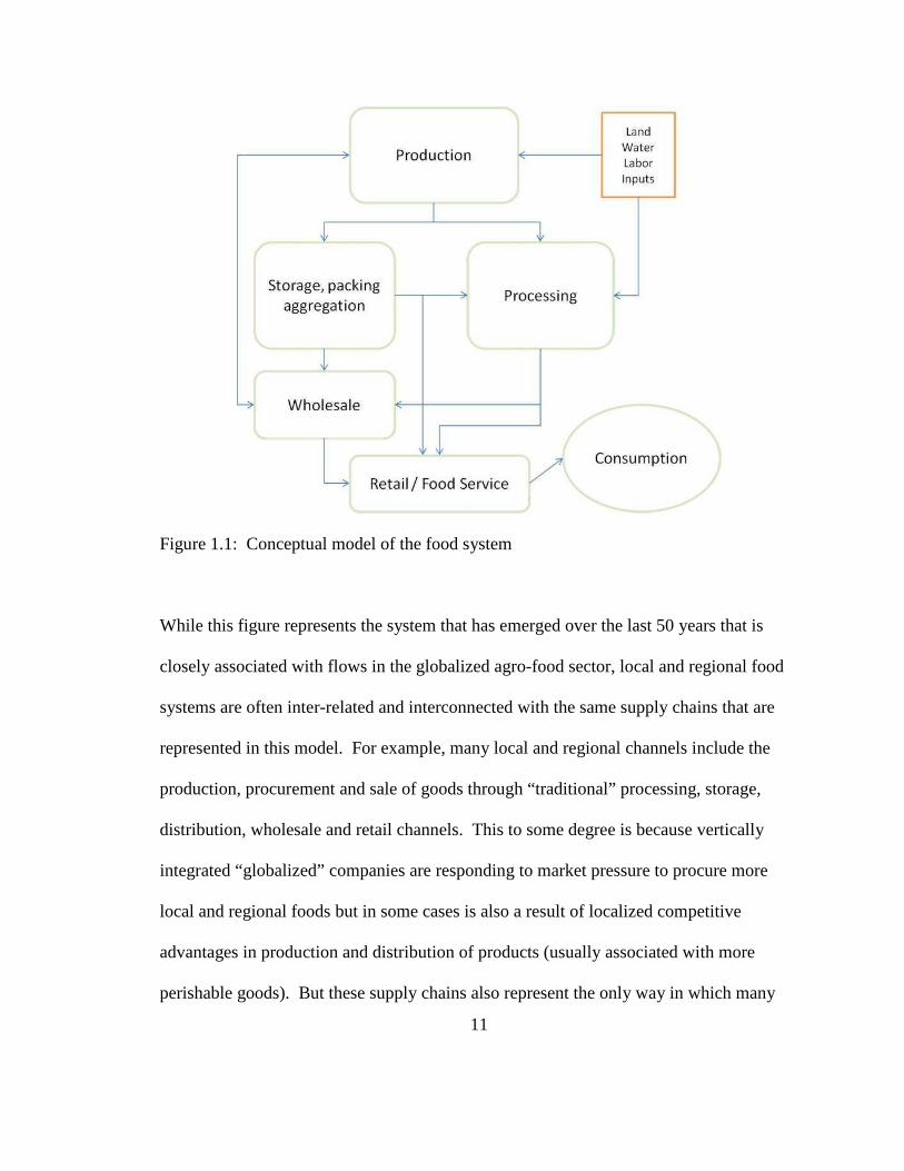
products experiencing dramatically different flows through the system. Figure 1.1
represents the core food system components and product flows of the present day food
system. The blue arrows represent some form of distribution. Many components
actually may function on multiple tiers of the model depending on supply chains and
integration of participating firms (e.g., many vertically integrated food retailers have
systems in place that capture the procurement mechanisms within the system such as
distribution, aggregation and in some cases even processing). Omitted from this model
are aspects of food management, safety and waste management.
11
Figure 1.1: Conceptual model of the food system
While this figure represents the system that has emerged over the last 50 years that is
closely associated with flows in the globalized agro-food sector, local and regional food
systems are often inter-related and interconnected with the same supply chains that are
represented in this model. For example, many local and regional channels include the
production, procurement and sale of goods through “traditional” processing, storage,
distribution, wholesale and retail channels. This to some degree is because vertically
integrated “globalized” companies are responding to market pressure to procure more
local and regional foods but in some cases is also a result of localized competitive
advantages in production and distribution of products (usually associated with more
perishable goods). But these supply chains also represent the only way in which many
12
local producers can get their product to local markets. Not all local and regional foods
however go through these more traditional supply chains and many local and regional
products are often associated with shorter supply chains or even sold directly to
consumers. So what exactly are local and regional foods and how do we know a local
and regional food system when we see it?
A multitude of actors participate in the food system in the Portland Metro Region, many
of whom are agnostic about both the geographic origin and location of final sale of their
products. Food system firms include producers, processors, aggregators and packers,
distributors, institutions, food service and retailers. The majority of these firms cannot be
conveniently partitioned into the distinct categories of local and non-local and
disaggregating the local products from the aggregated supply chains is challenging.
Traditionally, the smaller, locally based firms were more likely to handle products that
were produced and sold locally however in recent years, because of the growth in
popularity of local and regional foods, even the larger, vertically integrated multi-national
conglomerates are sourcing (and selling) local and regional products. For example,
during the summer season, locally sourced produce accounts for 20% of produce
available at WalMart and 30% of produce available at Safeway (Martinez, 2010).
Presumably, these products pass through these companies’ regional distribution centers.
The conflation of local and non-local products among firms occurs primarily within the
intermediaries in the supply chain. For example, according to a survey conducted by
13
Ecotrust (2013) of local and regionally focused distributors in the Portland Metro Area
(see Chapter IV for more detail), all were dedicated to local and regional sourcing of
products; however, none were able to exclusively source locally. The proportion of local
and regional produce ranged from 25% to 80% (during the growing season). These firms
relied on imported products for the success of their businesses, particularly during the
winter months. Likewise, processing facilities have been unable to source exclusively
from local producers because the supply of product is too inconsistent.2
While extensive literature has emerged that has attempted to define local and regional
food systems, no single agreed-upon definition currently exists. The concept of local and
regional food systems emerged for the most part in the late 1990’s, largely presented as
an alternative to the undesirable effects of the globalized food system. These early
scholars articulated alternative food systems as being distinct from the global food system
but much of this work was focused on describing specific case studies or systems that
represented niche markets or supply chains. Murdoch (2002) questioned the degree to
which these alternatives described by many researchers actually created a new structural
configuration.
Furthermore, a primary distinction of these alternative systems included aspects of
shortened supply chains. Inherent in this is the concept of re-spatialization of food
supply chains by which local food became a poster child for the alternative movement.
2 Information derived through my participant observation (see Chapter IV for more detail)
14
However, the perceived social and environmental outcomes associated with sustainable
agriculture (and by extension alternative food systems) should not necessarily be
confused with outcomes of a more local and regional food system. This is what Born and
Purcell (2008) refer to as the “local trap”. The local trap refers to the tendency of food
activists and researchers to assume something inherent about the local scale. However,
local food system advocates as well as researchers and economic development
professionals continue to tout potential benefits that can stem from re-localizing food
systems. I argue, the terms “local” and “alternative” are often used interchangeably
however care must be taken not to confuse the two. The term alternative refers to an
alternative to something. Sonnino and Marsden (2006) point out that such alternative
definitions are variously and loosely defined in terms of “quality”, “transparency”, and
“locality”, and that such newly emerging networks are signaling a shift away from the
industrialized and conventional food sector, towards a re-localized food and farming
regime. While there are elements of this definition that are inherently local, “local” food
systems as defined by many do not necessarily always exhibit the characteristics of
“alternative” systems identified by the social theorists who have juxtaposed alternative
systems as a form of resistance to the global agro-food industry. Here in lies a
fundamental distinction between definitions of local and regional foods. On the one
hand, a purely geographic definition describes local and regional foods as being produced
within some specified distance (or other geographic measure) of where the food is
ultimately consumed. The geographic definition of local and regional foods is subject to
the “local trap” described above. Food may be produced and consumed within the same
15
geography or region with the consumer knowing nothing about the food’s source or
practices used to produce it. It may very well be that these local foods are being
produced by large-scale, export-oriented operations held by multinational corporations
that do little to support local economies, the environment or community well-being.
A qualitative definition of local and regional foods however incorporates the alternative
system into a spatial framework. That is, the qualitative definition of local and regional
foods is a subset of the geographic definition in which products consumed are produced
locally AND are embedded with information pertaining to the source and production
practices. The consumer is consuming not only food but aspects specific to the quality,
nature and authenticity of the food itself. They do so by interacting with the producers
themselves (through directly marketed channels) or through some “trusted” source that
preserves some transparency specific to the supply chain of the product (intermediated
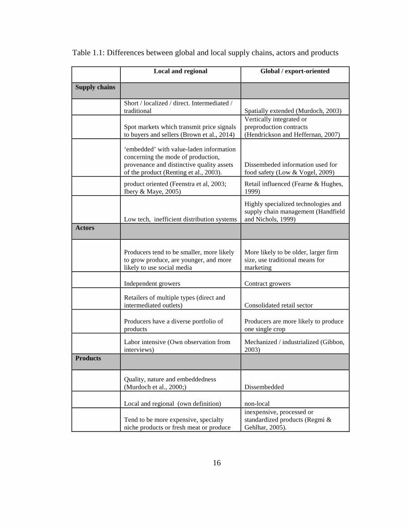
channels). Table 1.1 shows some of the primary differences between local and regional
food systems and the global, export-oriented, agro-food industry. In some cases, the
distinctions apply to the differences between the qualitative definition of local and
regional food systems and the export-oriented food systems and in some cases, the
distinctions may apply to both the geographic and qualitative definitions.
16
Table 1.1: Differences between global and local supply chains, actors and products
Local and regional Global / export-oriented
Supply chains
Short / localized / direct. Intermediated / traditional Spatially extended (Murdoch, 2003)
Spot markets which transmit price signals to buyers and sellers (Brown et al., 2014)
Vertically integrated or preproduction contracts (Hendrickson and Heffernan, 2007)
‘embedded’ with value-laden information concerning the mode of production, provenance and distinctive quality assets of the product (Renting et al., 2003).
Dissembeded information used for food safety (Low & Vogel, 2009)
product oriented (Feenstra et al, 2003; Ibery & Maye, 2005)
Retail influenced (Fearne & Hughes, 1999)
Low tech, inefficient distribution systems
Highly specialized technologies and supply chain management (Handfield and Nichols, 1999)
Actors
Producers tend to be smaller, more likely to grow produce, are younger, and more likely to use social media
More likely to be older, larger firm size, use traditional means for marketing
Independent growers Contract growers
Retailers of multiple types (direct and intermediated outlets) Consolidated retail sector
Producers have a diverse portfolio of products
Producers are more likely to produce one single crop
Labor intensive (Own observation from interviews)
Mechanized / industrialized (Gibbon, 2003)
Products
Quality, nature and embeddedness (Murdoch et al., 2000;) Dissembedded
Local and regional (own definition) non-local
Tend to be more expensive, specialty niche products or fresh meat or produce
inexpensive, processed or standardized products (Regmi & Gehlhar, 2005).
17
My quantitative and spatial analysis for the Portland area focuses on producers who sell
locally through any channel. That is, in the analysis I am interested in actors producing
local food rather than actors participating in local food supply chains. I conducted this
analysis by drawing on a dataset derived from a survey that explicitly asks a series of
questions of producers specific to the geographic distribution of their product in addition
to marketing channels. In this sense, the analysis uses the geographic definition of local
and regional food systems described above. My qualitative analysis on the other hand
focuses on producers who marketed their products through specific supply chains. I
therefore am able to explore aspects of agglomeration forces specific to the qualitative
definition of local and regional food systems.
1.3: GROWTH OF LOCAL FOOD
Growth of both the popularity in the concept of local and regional food as well as the
actual sales of local and regional food products that are directly marketed has been on the
rise. Furthermore this growth has been a recent phenomenon. While historic data
pertaining to local and regional food supply chains is limited to case studies, data does
exist that describes the growth at the firm level. Perhaps the best indicator of growth of
the local and regional food sector can be accounted for in the final sale of local and
regional products through direct markets.
Data on direct-to-consumer food sales were first collected in the 1978 Census of
Agriculture, after the Farmer-to-Consumer Direct Marketing Act was passed (Low and
18
Vogel, 2011). Multiple other sources exist that collect data specific to the number of
outlets by marketing channel as well. Direct-to-consumer marketing amounted to $1.2
billion in sales in 2007, compared with $551 million in 1997 (USDA, 2007). In the
Portland Metro Region of Oregon, there was also a sharp increase from 2002 to 2007 in
the proportion of sales through direct channels. The USDA Census of Agriculture
reported a total of 1,245 farms or 19.29% of all food farms in the Three County Region
(i.e., excluding products such as hay, Christmas trees, or ornamentals) reported direct to
market sales. Furthermore, total direct to consumer sales increased by 87.1% from 2002
to 2007 in the Three County Region.
The number of direct to consumer outlets has been on the rise as well. Farmers’ Markets
voluntarily listed in USDA National Farmers Market Directory are up more than 400%
from 1994 (1,755) to 2013 (8,144). CSAs were first established in the U.S. in mid-1980s
with 2 operations. In the 2007 Census of Agriculture, 12,549 farms reported they had
marketed products through CSAs or some form of subscription agriculture arrangement.
There has been an increase in sales and the number of outlets in the intermediated
channels of local and regional food as well. The number of farm to school programs,
which use local farms as food suppliers for school meals programs, increased to 2,095 in
2009, up from 400 in 2004 (Low and Vogel, 2011). The growth can be seen in the
popularity of locally sourced products in major retail establishments as well. For
19
example, several leading retailers have recently announced local food initiatives
including WalMart, Safeway, Kroger and Ahold (Martinez, 2010).
In the Portland Metro Area, all of Portland’s farmers’ markets (14 in all) with the
exception of Portland Farmers’ Market now located at Portland State University, have
opened since 1994. In 2007, there were 37 farmers’ markets in the Three County Region,
compared to just four in 1994 (Oregon Farmers Market Association, 2013). CSA’s have
also increased dramatically in the last 20 years. The first CSA’s were started in the
Portland Metro Region in the 1990’s (Portland Area Community Supported Agriculture
Coalition). The City of Portland’s Bureau of Planning and Sustainability maintains a list
of self-reported CSA’s. Currently there are over 50 CSA’s listed in the region.
Considering a substantial amount of local and regional products pass through
intermediated channels (Low and Vogel, 2011), and that tracking trends in these channels
is difficult, there is insufficient evidence to point to the growth of local and regional
foods in terms of its geographic definition. It may very well be that recent introduction
of local produce in major retail establishments is merely a function of daylighting pre-
existing supply chains to take advantage of the perceived benefits of local foods. It may
also be that the amount of local and regional products passing through intermediated
channels is in decline as more local and regional producers forego these channels to take
advantage of direct to consumer supply chains. In this sense, the above trends indicate
that there has been substantial growth specific only to the qualitative definition of local
20
and regional foods and that it is the practice of selling food embedded with information
and economic and social relations that constitutes a new and growing sector.
1.4: GEOGRAPHIC SCOPE
The geographic scope of the research presented here is conceptualized at the regional
scale. The growth of cities is directly related to, affect, and are affected by their peri-
urban and rural counterparts. Economic activity plays out at the regional scale. When
considered as a system, the new food economy unfolds at the regional scale as well. For
example, given concepts of localization, embeddedness, and food geographies, both the
supply of food products and the demand for those products are regional in scale.3
Furthermore, agglomeration economies are regional and benefits of both localization
externalities and urbanization externalities can affect how systems organize. My unit of
analysis therefore is the Portland Metro Region of Oregon. And while I will draw on
descriptions of the new food economy in regions throughout North America and Europe,
I have defined my region of interest for this analysis as the three counties in Oregon that
have strong connections in terms of food product flows to the core metro area of
Portland. These include Washington, Multnomah and Clackamas counties (Map 1.1).
While together these counties represent a significant proportion of the state’s agricultural
production, they also are the three most urbanized counties in the state (U.S. Bureau of
Census 2010). Combined, the three counties represent nearly 43% of the state’s total
3 While there is no clear definition of exactly what constitutes local in term of food production, given the unit of analysis presented here is the region, the definition stems from that unit. That is, I only consider food that is produced sold within the region to be local and regional and while food from outside the region, under many definitions, may be considered local and regional, it is not considered in this analysis.
21
population and are home to three of the State’s five largest cities (U.S. Bureau of Census
2010).
In terms of agricultural output, Oregon is the 28th largest producer of agricultural
products in the United States and nearly 45% of all agricultural revenues originate from
the Willamette Valley. Furthermore, of the top five counties in terms of revenue
associated with agricultural products, Clackamas, Washington and Multnomah are 2nd,
4th and 5th respectively (USDA NASS 2007).
Figure 1.2: Map of Portland Metro Area and the Three County Region
22
Agriculture products are among Oregon’s major industries accounting for 9% of
Oregon’s gross state product and 8% of all Oregon jobs (US Bureau of Labor and Statics
2008). In 2010, Oregon produced $3.75 billion in total agricultural output, and the Three
County Region accounted for roughly 20% of this total ($793,244,000) (USDA NASS
2008). Oregon exports roughly 35% of its total agricultural output in value ($1.32
billion) and represents 100% of the nation’s output for blackberries, hazelnuts and two
different types of grass seed (ryegrass and fescue) all of which originate in the Willamette
Valley (USDA ERS 2010).
While the Three County Region is a major exporter of many agricultural products (for
example nursery stock and Christmas trees as well as many types of berries), it also
grows a significant amount of food products that are sold locally relative to other regions
in the Country4. In Portland, a dedicated focus on building rural-urban connections
emerged among food system activists in the 1990s, with organizational leaders that
included Portland Farmers Market, Food Alliance, Portland Chapter of the Chefs
Collaborative, New Seasons Market, Burgerville, Kaiser Permanente, Ecotrust, and many
others (Halweil 2004). The success of these establishments and the social and
environmental values of which they embody, have led regional leaders to take a close
look at concepts around local food as a regional economic development strategy. For
example, both Multnomah County and Clackamas County have begun to investigate how
fostering a regional and local food system “cluster” could contribute to economic
4 USDA NASS 2007 Census of Agriculture reported that nearly 4% of food products grown in the Three County Region were directly marketed to consumers relative to <1% nationally.
23
development.5 Given the unique agricultural landscape in the Three County Region, and
the dense urban population, coupled with the region’s history of land use planning laws
that allow for the persistence of farmland close to the urban core,6 the study area is an
ideal setting to understand potential implications of the new food economy in the context
of the city-region.
While my descriptive and qualitative analyses both focus on the broader Three County
Region, my quantitative and spatial analyses focus on Clackamas County alone.
Clackamas County represents a significant proportion of agricultural output in the region
($397,318,000 relative to Multnomah County: $84,546,000 and Washington County:
$311,380,000) and produces the majority of all vegetables ($19,212,000 relative to
Multnomah County: $11,774,000 and Washington County: $6,874,000) (USDA NASS
2007). Map 1.2 shows Clackamas County agricultural lands and parcels that produce
food products on at least a proportion of their land. Furthermore the County is actively
pursuing a variety of strategies to try and foster local and regional food supply chains.
As part of the County’s strategy, it developed the Clacakamas County producers survey,
of which I have drawn from extensively to both differentiate local and regional food
producers from export oriented producers and conduct my spatial analysis presented in
chapter V.
5 The Multnomah food initiative and the Clackamas County Agricultural Opportunities Assessment are both recent programs that exemplify this focus. 6 Oregon adopted growth management legislation in 1973 and Portland’s UGB was proposed in 1977 and approved by
the state in 1980
24
Figure 1.3: Map of Clackamas County Agricultural and Food Production Lands
1.5: THEORETICAL FOUNDATIONS
Although the research presented here does not attempt to expand on any specific body of
theory, it is not without its theoretical foundations. On the contrary, I have drawn upon
the theoretical foundations of industry life cycle, political economy, endogenous growth
theory, and theories stemming from the knowledge geography literature to formulate my
hypotheses and construct a sound methodology for data analysis.
25
To help differentiate the local regional food system from the export oriented food system
I have drawn extensively from the theoretical underpinnings originating from the agro-
food literature. These stem from three dominant theories: political economy which
situates the food regime as partly about international relations of food, and partly about
the world food economy and regulation of the food regime underpins and reflects
changing balances of power among states, organized national lobbies, classes—farmers,
workers, peasants and capital (Friedmann, 2005); rural sociology which contextualizes
alternative systems as a form of resistance against the globally connected, agro-food
industry and the failures of that system and; actor network theory (e.g. Murdoch et al.
2000; Goodman 2003; Selfa amd Qazi 2005) in which localized forms of food systems
are defined by the value of the networks and the relative importance of how actors in the
system construct notions of local. I draw on each of these theories to characterize
differences between the global and local food systems. However, while the theories of
political economy, rural sociology, and actor network theory all play a key role in
formulating the hypotheses and contextualizing the concept and motivations behind the
emergence of the new food economy, as well as highlighting key differences between the
systems, my motivation behind this specific line of inquiry stems from the fields most
concerned with economic interactions that are constrained by geographic space and
unfold at the regional scale.
Ultimately, the theoretical lens for this research draws from theories that have arisen from
the fields of Economic Geography and Regional Science. Within Economic Geography,
26
I situate my analysis by drawing from those theories concerned with economic growth at
the regional scale including endogenous growth theory and theories of agglomeration
externalities. Endogenous growth theory - postulated by Paul Romer (1994) and Robert
Lucas (1988) - is concerned with the development of regions through endogenous forces
such as human capital, knowledge spillovers and innovation rather than exogenously
through demand for exports. Agglomeration theories attempt to explain the clustering of
activity as a result of positive externalities associated with labor pooling, specialized
services, urbanization externalities and knowledge spillovers.
Closely related although more focused on methods rather than theoretical constructs is
the field of Regional Science. Walter Isard in his book Location and Space Economy
(1956), details historic lines of thought pertaining to general theories applicable to what
would ultimately become the field of Regional Science. Central to Isard’s theories are the
works of three German economists who between them describe the foundational spatial-
economic interactions pertaining to regions: Von Thünen’s isolated state theory builds on
work by Adam Smith to conceptualize how a farmer is expected to maximize his profit
from his farmland; Walter Christaller’s, central place theory builds on Von Thunen's
work to describe how regions grow and are arranged in a spatial context, specifically how
goods and services flow within regions and; Alfred Weber’s theory of industrial location
tries to explain and predict the location patterns of industry at a macro-scale. Together
these three theories provide explanations for where a firm will locate, what the value of
land will be, and how regions grow. All three are drawn from (and prove to be
27
interrelated) by Isard in his formulation of his general theory relating to industrial
location, market areas, land use, trade and urban structure. And all are pertinent to the
concept of how the new food economy emerges at the regional scale.
Each of these disparate bodies of theory provides the foundation for my analysis. And I
draw from the broad set of methodological tools offered by these fields. In the next
section I turn to a general overview of my approach, saving the detail of exact
methodologies for subsequent chapters in which the associated analyses are presented.
1.6: CONCLUSION
Economic development professionals, city and regional planners, decision makers and
food policy advocates are all grappling with ways in which to foster local and regional
food systems for a multitude of reasons. Many of these efforts are focused on expanding
existing clusters of economic activity for the purpose of regional and or rural economic
development. However, research pertaining to the benefits of local and regional food
systems specific to economic development is largely lacking and currently little evidence
exists to support rational investment and intervention strategies to foster the new food
economy. Building on the wide body of literature pertaining to alternative food systems,
and bridging it with the literature specific to Regional Science and Economic Geography,
the research presented here aims to construct a theoretical framework that situates the
new food economy within the context of the city-region. This framework can be used to
support future research for identifying whether new food economies represent an
28
opportunity for regional economic development and will result in evidence that can serve
as a key foundational building block on which to begin to understand strategies for
fostering these new food economies.
The structure of this dissertation is as follows: In the next chapter (chapter II) I present a
literature review of the foundational and substantive works pertaining to the disciplines of
agro-food systems research, Regional Science and Economic Geography – focusing on
aspects of economic development and agglomeration economies and works stemming
from the knowledge geography literature. In chapter III, I provide an historical overview
of the evolution of food systems and agriculture in the Portland Metro Region and detail
the present day structure, paying close attention to the economic, policy and land use
drivers that have set the stage for the emergence of the new food economy in its present
state. In chapter IV, I give a detailed overview of my methods and the data used in my
analyses and then in chapters V and VI, I present my spatial and qualitative analyses in
which I test hypotheses specific to the spatial structure of local and regional food systems
and the processes of knowledge accumulation. Finally in chapter VII, I consider the
implications of the new food economy in terms of regional economic development and
discuss existing barriers and constraints to the emergence of such a system specific to the
two definition presented above before concluding with thoughts on possible future
directions of the system and future research needs.
29
CHAPTER II : LITERATURE REVIEW
2.1: OVERVIEW
I focus my literature review on three distinct bodies of research: the agro-food systems
literature, Regional Science and New Growth Theory. My review of the agro-food
literature provides a theoretical background for describing the existing agro-food
structures both in terms of the characteristics of the dominant regime of the export-
oriented, globally linked agro-food sector as well as the reasons for the emergence of the
new food economy; the New Growth Theory literature helps me frame my hypotheses
and provides a theoretical foundation for contextualizing the emergence of the new food
economy in terms of the city-region and; the Regional Science literature both supports
the theoretical foundations presented by the New Growth Theorists as well as provides a
framework for both my quantitative and spatial analyses. In this chapter, I provide an
overview of each of these distinct bodies of literature and then discuss some of the
theoretical applications of economic development for local and regional food systems
before concluding with an overview of some recent works that have attempted to measure
the impacts of local and regional food systems at the regional scale.
2.2: LOCAL AND REGIONAL FOOD SYSTEMS AND AGRO-FOOD
RESEARCH
The research stemming from the agro-food literature draws on a wide array of theoretical
frames including social theory and economic sociology (Kloppenberg et al. 1996;
30
Murdoch et al. 2000; Hendrickson and Heffernan 2002; Hinrichs 2003; Jaroz 2008), actor
network theory (Goodman 1999; Murdoch et al. 2000; Selfa amd Qazi 2005) and
political economy (Murdoch et al. 2000; Allen et al. 2003; Winter 2003) among others.
Some of the themes that have emerged in recent research elucidate concepts presented by
social theorists such as David Harvey (1996) pertaining to consequences of modernity
and post-modernity and situate alternative systems as a form of resistance to the modern
globally connected agro-food industry. This resistance involves the emergence of
alternative systems defined by themes such as embeddedness, quality, stronger social
connections and connections with nature.
Political economy is often used to describe the existing structure that has emerged as the
dominant regime. The food sector has gone through a broad shift to transnationalization
and globalization and has been integrated into a set of transnational and transectoral
production process (Murdoch et al.2000). Political economy has been used to both
describe this process (Hendrickson et al. 2001) as well as contextualize some of the
consequences of this integration (Mardsen 1988; Friednalnd et al. 1991; McMichael
1994).
Social theory and economic sociology is used extensively throughout the agro-food
literature as a way to situate alternative food structures as a form of resistance to the
globalized systems. For example Hendrickson and Heffernan (2002) argue that food
system alternatives challenge the time space distantiation that characterizes the
31
continuing development of the dominant agro-food system. Local food has recently
emerged as a banner under which people attempt to counteract trends of economic
concentration, social disempowerment and environmental degradation resulting from the
globalized agro-food regime (Hinrichs, 2002). At the center of this discourse is the local
as a place for connections and resistance. For example, Allen et al. (2003) attest that
people are working to construct new initiatives that challenge the existing food system.
Localizing food seems to manifest both oppositional and alternative desires, providing an
opportunity for directly personal relationships between producers and consumers. They
apply concepts articulated by Harvey (1989) such as alternative, oppositional, militant
particularism and global ambition to examine the local as a site of resistance.
However, the local as a site of resistance has been conflated with local as a geographic
specifier and the assumption that local alone can solve the problems resulting from the
failures of the globalized system should be questioned. Recent research interrogates
whether and to what degree this new food paradigm addresses the objectives of social
justice and inclusion, ecological sustainability and economic viability (Jarosz 2008). Born
and Purcell (2008) argue that local food systems are no more likely to be sustainable or
just than systems at other scales. They use scale theory to frame their argument that scale
is socially produced: scales (and their interrelations) are not independent entities with
inherent qualities but strategies pursued by social actors with a particular agenda.
Goodman (2004) argues that the spatial content of local contexts needs to be more
critically examined both to take account of how scale is socially constructed and to
32
understand how social and environmental relations are themselves spatialized. In this
sense, much work is still required to better understand and evaluate the roles that regional
food systems might play in providing for social and natural wellbeing (Martinez et al.
2010).
What have emerged in the literature are two distinct concepts of local food. On the one
hand there exists a geographic definition articulated by the proximity of production and
consumption. On the other hand is a more qualitative definition articulated by themes
such as embeddedness, quality, stronger social connections and connections with nature.
The qualitative definition may also encompass aspects of defensive localism. For
example Winter (2003) found considerable evidence of an ideology of localism based on
sympathy for farmers. That is, the turn to local food may cover many different forms of
agriculture, encompassing a variety of consumer motivations and giving rise to a wide
range of politics (Winter, 2003).
2.3: INSTITUTIONAL STRUCTURES AND THE GLOBALIZED AG RO-FOOD
SYSTEM
In this section I highlight literature that has attempted to characterize some of the more
dominant trends in food systems more broadly. Food systems have gone through
tremendous transformation in the last 50 years. And through this transformation the
global system has emerged. Depending on the frame of reference, this transformation has
been called a variety of terms such as processes of agricultural industrialization (Parrottet
33
al., 2002), or productivism (Ilbery and Bowler, 1998). Regardless of the nomenclature
used, the transformation has been marked by three major trends: 1) rapid advances in
transport and communication technologies; 2) increase in processed and manufactured
products and; 3) substantial consolidation and vertical integration of food system
conglomerates particularly within both the production and retail sub-systems.
2.3.1: Distribution and information technology
The growing flows of freight have been a fundamental component of contemporary
changes in most economic systems at the global scale (Hesse & Rodrigue, 2004) and
food systems are no exception. Advances in transport and communication technologies
have created new opportunities for the development and growth of multinational firms
within the food industry and now represents a significant sub-system within the
globalized agro-food sector.
Logistics consider the wide set of activities dedicated to the transformation and
circulation of goods, such as the material supply of production, the core distribution and
transport function, wholesale and retail as well as the related information flows
(Handfield and Nichols, 1999). The core component of materials management is the
supply chain, the time- and space-related arrangement of the whole goods flow between
supply, manufacturing, distribution and consumption. (Hesse & Rodrigue, 2004). With
the coupling of information technology, marketing and strategic planning with
distribution and materials management, logistics has evolved into supply chain
34
management. The flow-oriented mode of corporate management and organization
currently affects almost every single activity within the entire process of value creation in
the globalized agro-food system (Lummus and Vokurka, 1999).
Management of supply chains that carry food products, particularly perishable products,
have had to respond to the growing demand for year around products. There is now a
considerable supply variation due to seasonality of agricultural production, weather
conditions, and the biological nature of agricultural products, which results in input
variation and unpredictability (Henson and Reardon, 2005). Vertical alliances have
emerged that often aim to smooth supply variation and guarantee the planned delivery of
supplies (Mangina & Vlachos, 2005). Coupled with increased competition these logistics
alliances have resulted in considerable structural changes in food supply chains (Clark &
Hammond, 1997; Fearne & Hughes, 2000). For example, automatic stock replenishment
and deliveries are increasingly becoming the responsibility of retailers such as WalMart
in the United States and Tesco in the UK (Mangina & Vlachos, 2005).
Information technology in most major agro-food sector corporations is integrated with
every function of the business. Supply chain management and information technology
departments often consist of enterprise technology services, IT program management, IT
sales, marketing, IT Corporate and Commercial Systems and Services and IT Supply
Chain Systems and Services (ConAgra, 2013). Such technologies act as a barrier to entry
for many producers and retailers.
35
2.3.2: Processed and manufactured foods
The last three decades have seen tremendous growth in sales of processed food—sales
now total $3.2 trillion, or about three-fourths of the total world food sales (Regmi &
Gehlhar, 2005). The increase in sales in processed and manufactured foods has led to
increased competition as agro-food businesses compete for increased market shares of
this rapidly growing sub-sector resulting in consolidation and strategic alliances (see
section 5.3.3). In the United States, the food manufacturing industry is one of the largest
manufacturing sectors, accounting for more than 10 percent of all manufacturing
shipments (BEA, 2012). The farm share of the “market basket” (i.e. non-processed foods)
remained stable at about 40% from 1960 to 1980 but declined rapidly since then, to 30%
in 1990 and 22.2% in 1998 (Sexton, 2000). The processed food industry has experienced
fairly steady growth over the 1997-2006 period. In 2006, the value of processed food
shipments from the U.S. was $538 billion, an increase of 27 percent from 1997 shipments
(U.S. Census Bureau, 2013).
2.3.3: Consolidation and vertical and horizontal integration
Consolidation is perhaps one of the most relevant aspects of recent trends in globalized
food systems. There were 316 total acquisitions in 2012 in the broader food and
beverage industry, and food processors constituted nearly ¼ of these acquisitions with 83
total mergers (Food Institute, 2013). This consolidation has occurred both at the national
as well as multinational level. Within the United States, perhaps the most striking forms
36
of consolidation can be seen in retail activity whereas multinational activity is a relevant
and an increasing phenomenon in food manufacturing (Senauer & Venturini, 2005).
The last 20 years in particular has seen a marked increase in consolidation activity in the
retail sub-system of the globalized agro-food sector through horizontal integration where
major retail establishments compete for market share through acquisition of companies in
geographically distributed markets. Currently the top five retail establishments represent
over 57% of all retail sales in the United States up from 48% in 2006 (the top four stores
- Tesco, Sainsbury's, Asda, Safeway - account for almost two-thirds of grocery sales in
the UK). Table 5.1 shows the market share of the top five retailers from 2004 to 2012.
Table 2.1. Top retail establishments sales 2004-2012 ($1,000)
Store 2012 2006 2004
WalMart $118,725,880 $98,745,400 $66,465,100
Kroger $61,128,860 $58,544,668 $46,314,840
Safeway $35,504,560 $32,732,960 $29,572,140
Supervalu* $28,229,188 $36,287,940 $31,961,800
Ahold $26,162,500 $23,848,240 $25,105,600
Source: Hendrickson and Heffernan, 2007 and Progressive Grocer’s Super50, 2012 *Supervalu purchased 40% of Albertson’s in 2006. 2004 and 2006 data represent Albertson sales
During the 1990s, supermarkets in the United States and throughout Europe shifted to
reliance on a relatively small number of specialized importers, rather than on traditional
wholesale markets. Importers were expected to engage in active global procurement, as
37
well as to organize the provision of a series of new services that supermarkets required
(Gibbon, 2003).
Retail growth strategies based on location and size (product range and price
competitiveness) have been replaced by strategies based on differentiation such as own
label fresh produce and meat (Fearne & Hughes, 1999). Buyer-driven chains link large
retailers and branded marketers to decentralized networks of producers of low-cost
developing countries (Gibbon, 2003). Buyer-led chains are actively driven in the sense
that large retailers and branded marketers use them not merely to source products, but
increasingly also to reshape their own portfolios of functional activities and to achieve
higher levels of flexibility (Senauer & Venturini, 2005).
As with retail, the production sub-system has seen significant consolidation and strategic
alliances. Hendrickson and Heffernan (2007) identify three major food chain clusters
that represent extensive vertical integration of production activities and account for a
major portion of global production of grain and animal feed. These include the
Cargill/Monsanto cluster, the ConAgra/Dupont cluster, and the Novartis
(Syngenta)/ADM cluster although since their research others may have emerged (e.g.
Smithfield and Tyson). These clusters assume control of food system activity from
genetic seed manufacturing to grain production through to grain collection, aggregation
and processing as well as meat production and processing. For example, ConAgra
purchases high-oil corn seed from DuPont; contracts with farmers to grow the corn; buys
38
it back for animal feed of which they control significant meat feed and processing
operations (the company produces its own livestock feed and ranks third in cattle feeding
in the U.S. and second in cattle slaughtering (Hendrickson and Heffernan 2007)).
In 2007, four firms controlled 60 percent of U.S. terminal grain handling facilities, with
Cargill having the most capacity, followed by Cenex-Harvest States, a farmer cooperative
with which Cargill has now embarked on a joint venture (Hendrickson and Heffernan
2007). Furthermore, With Cargill’s acquisition of Continental, it controlled more than 40
percent of all United States corn exports, a third of all soybeans exports and at least 20
percent of wheat exports. At the global scale, the merger combines what was reported at
the start of the 1990s to be the largest two global grain traders. The emergence of ADM
as a major global grain trader came through the acquisition of parts of Louis Dreyfus and
Pillsbury (Conner, 2003).
Processed foods have also experienced extensive consolidation in recent years. For
example, ConAgra, in 2013 completed a $4.95 billion acquisition of private-label food
maker Ralcorp making it the largest private label food maker in North America (Brown,
2013). ConAgra bought Ralcorp because of its dominating presence in the private-label
food space and now constitutes approximately $4.5 billion in combined annual private
label sales and about $18 billion in total sales. Private-label food sales currently make up
18% of U.S. food sales. (Ziobro, 2013).
39
Kellogg Company became the world's second-largest savory snacks company with the
$2.7 billion purchase of Procter & Gamble's Pringles brand in 2012, which earns $1.5
billion in sales across more than 140 countries (Food Institute, 2013). Campbell Soup Co.
acquired Bolthouse Farms for $1.55 billion, a vertically integrated food and beverage
company focused on high value-added natural products and in possession of significant
market positions in fresh carrots, premium beverages and private label products in the
U.S (Ziobro, 2013).
In 2013, the twelve largest U.S. companies in this sector were PepsiCo, Tyson Foods,
Nestle, Anheuser-Busch, Kraft Foods, General Mills, Smithfield Foods, Dean Foods,
Mars, Coca-Cola and ConAgra Foods (Food Processing, 2013). In 2012, Kraft Foods, the
largest in the industry at that time, employed 103,000 employees, had more than 180
manufacturing and processing facilities worldwide, and reported net revenues of $37
billion (Food Institute, 2013). Kraft currently manufactures some of the industry’s
leading brands, such as Oreo, Nabisco, Oscar Mayer, Philadelphia Cream Cheese, and
Maxwell House coffee.
In 2012 there was 266 percent increase in fruit and vegetable processor mergers. Tomato
producer Lipman bought Branscomb Produce, Combs Produce and the Ace Tomato Co.
packing house across the U.S. in California. In 2013, Seneca Foods also acquired an
ownership interest in Independent Foods, a Sunnyside, Wash.-based processor of canned
pears, apples and cherries (Food Institute 2013).
40
Meat production as well is marked by intense market concentration in which a very small
number of corporate packers accounts for the majority of meat that ends up in the grocery
store. In 2007, four corporations slaughtered 83.5 percent of the nation’s beef, 66 percent
of the pork and 58.5 percent of the poultry (Heffernan and Hendrickson 2007).
2.4: CONSEQUENCES OF GLOBALIZED FOOD SYSTEMS
The major trends in the food industry over the last 50 years has led to a broad shift
toward transnationalization and globalization that has been integrated into a set of
transnational and transectoral production process (Murdoch et al., 2000) and global
commodity chains. These global commodity chains are sector-based structures of
international trade, arising from the twin phenomena of dispersal of production (through
outsourcing) and market integration (through trade liberalization) (Gibbon, 2003). Like
processes of modernization, analysts see globalization in the food sector as derived from
agencies which aim to promote new inter-linkages between the principal actors (e.g.,
farmers, processors, and retailers), spread new uses and forms of knowledge (linked
especially to science and technology), and establish new commodity forms within mass
markets (Murdoch et al., 2000).
However, this globalization of the food system has led a growth of theoretical and
practical critiques of several distinct outcomes: an increasing exploitation of large
segments of society as manifested in increasing inequalities, poverty, hunger, poor health,
41
and loss of cultural diversity (Koc and Dahlberg, 1999); vulnerabilities “created by a
global economy operating in real time” (Gwynne et al., 2003), particularly the herd
behavior of investors and currency traders; and the undemocratic nature of the
governance of global capitalism (Watts et al., 2003); increasing exploitation of the
natural environment, which is manifested in increasing pollution, resource losses and
degradation, and loss of biodiversity (Marsden, 1994) and; an increasing loss of national,
state, and local political power as concentrations of economic and corporate power
increase, with a corresponding reduction of democratic power and social controls (Koc
and Dahlberg, 1999)
It is through these “cracks in the façade” (Leyshon and Lee, 2003) that local and regional
systems have begun to emerge as alternatives to the consequences of the global system.
For example Hendrickson and Heffernan (2002) argue that food system alternatives
challenge the time-space distantiation that characterizes the continuing development of
the dominant agro-food system. Local food has recently emerged as a banner under
which people attempt to counteract trends of economic concentration, social
disempowerment and environmental degradation resulting from the globalized agro-food
regime (Hinrichs, 2002). At the center of this discourse is the local as a place for
connections and resistance. For example, Allen et al. (2003) attest that people are
working to construct new initiatives that challenge the existing food system. Localizing
food seems to manifest both oppositional and alternative desires, providing an
opportunity for directly personal relationships between producers and consumers. They
42
apply concepts articulated by Williams and Harvey such as alternative, oppositional,
militant particularism and global ambition to examine the local as a site of resistance.
2.5: LOCAL AND REGIONAL FOOD SYSTEM STRUCTURES AND SUPPLY
CHAINS
Lack of a publicly recognized definition for “local food” presents a challenge for
identifying differences at the structural scale. Despite the growing use of the term “local”
in academic and civic discourse, there is no consensus on a precise definition. (King,
2010). As mentioned above, most theorizing pertaining to local and regional food
systems has stemmed from a reaction to the external costs of the global system. As such,
a wide variety of themes have emerged in the literature specific to aspects of local and
regional food that are distinct from that of the globalized system. Such themes include
elements of structure (Hendrickson et al, 2001; Hendrickson and Heferman, 2002;
Christopherson, 2006; Wrigley et al, 2005), scale (Born and Purcell, 2006) management
practices, authenticity and embededness (Watts, Ilbery, & Maye, 2005) and geography
(Selfa & Qazi, 2005; Martinez, 2012).
The structural differences between the local and global systems are best articulated
through definitions of supply chains. Local and regional food systems are an example of
where short supply chains present a spatial alternative to conventional supply chains (e.g.
Renting et al., 2003). Using a strictly geographic definition, local food refers to food
produced near its point of consumption in relation to the modern or mainstream food
43
system (Peters et al., 2008). In this sense, the geographically defined of local food may
very well travel through traditional supply chains.
The structural configuration of supply chains associated with the qualitative definition
however is slightly different. What is unique about these local supply chains is that
information must be conveyed about the product that enables consumers to recognize it
as a local food product. That is, local food supply chains strive to establish a bond
between the producer and the consumer, even when separated by intermediary segments
in the supply chain (Renting et al., 2003). Marsden et al. (2000), describes three types of
localized food supply chains: face-to-face, where consumers buy a product direct from
the producer/processor on a face-to-face basis; spatially proximate, where products are
sold through local outlets in the area and consumers are immediately aware of its local
nature and; spatially extended, where products are sold to consumers who are located
outside the local area and who may have no knowledge of that area. Here, the key is to
use product labeling and imagery to transfer information about the production process
and the area to the consumer (Ilbery et al., 2003).
A body of research has also emerged specific to producers selling their products locally.
Here, most research can be placed under the geographic definition of local and regional
food systems as differentiating the supply chains associated with the producers is
challenging. King et al. (2010) found that at the national scale, farms that participate in
local food supply chains relative to export-oriented farms have a more diverse portfolio
44
of products and market outlets. They showed that small farms may diversify product
offerings to defray large fixed costs across multiple sources of revenue, or they may use
multiple types of local market outlets. Outlets used by local and regional food producers
include direct to market channels including farmers’ markets, roadside stands, on-farm
stores, and community-supported agriculture arrangements (CSAs) and intermediated
marketing channels including sales to regional distributors and grocery stores,
restaurants, or other retailers (Martinez, 2010). A small portion of local and regional
foods is also sold through institutional channels such as through farm to school programs.
In 2007, more than half of U.S. local food sales were from farms selling exclusively
through intermediated marketing channels such as grocers, restaurants, and regional
distributors. Farms using both direct-to-consumer and intermediated marketing channels
accounted for a quarter of local food sales ($1.2 billion). Only $877 million (roughly
18%) was generated by farms that participated exclusively in direct to consumer sales
Next, I turn my attention to literature specific to the fields of Regional Science and
Economic Geography. I highlight these fields because I use the theoretical and
methodological formulations to investigate the evolution of the new food economy in
terms of the city-region. First, I focus on the foundational scholars of Regional Science,
for the most part because it is these foundational thinkers that provide the contextual
framework for the theories of economic development and New Growth Theory from
45
which I draw to formulate my hypotheses. Additionally, the field of Regional Science
has given birth to advanced methods of regional analysis, including approaches to
measuring aspects of agglomeration economies. I draw on these methods to perform my
spatial analysis presented in Chapter V. Central to Regional Science is the concept that
geographic space matters. Aspects of the effects of geographic space are addressed in all
of the theoretical underpinnings of the field and many of the methods are concerned with
how to incorporate space into analytical techniques. I focus my review of Regional
Science specifically on location theory and methods of regional and spatial analysis,
primarily because it is these arenas within the field of Regional Science that provide a
useful lens through which to evaluate aspects of the new food economy that I outlined
above.
Location theory is concerned with the macroeconomics of space. Broadly speaking,
location theory provides the theoretical foundations for a wide array of topics including:
analysis of land use patterns and urban form, spatial interaction, spatial diffusion, trade
area analysis, location of decisions of the firm and industrial location analysis, location of
service centers and network analysis. While aspects of regional growth and urban form
related to Walter Christaller’s central place theory, as well as aspects of New Growth
Theory are closely related to - and in many respects subsets of - location theory, I will
address each of these in later sections. Here I focus on location theory as the basis for
locational decisions.
46
Location theory was originally developed because of the recognition for incorporating
transportation costs into price theory. Transportation costs are different from other
production costs because they can impose certain recurring types of spatial arrangements.
Beckmann (1999) identifies two ways in which geographic space affects economic
relationships: through the uneven distribution of natural resources and through distance
separating economic activities. Distance separating activities can be thought of both in
terms of how economic activities affect other activities carried out in adjacent locations
(neighborhood effects) as well as costs incurred by moving goods (transportation costs).
These concepts are the articulation of many of the works outlined above however the
work of Alfred Weber and his theory of industrial location (1909) which tries to explain
and predict the location patterns of the industry and Von Thunen’s isolated state theory
(1826) provide the backbone of this sub-field of Regional Science. Weber’s theory
emphasizes that firms seek a site of minimum transport and labor cost whereas Von
Thunen’s theory attempts to explain the value of land (and subsequent land use patterns)
based on the distance to a marketplace. Whereas Weberian models are concerned with
facility location, Von Thünen based models are interested in the spatial variation of
phenomena across geographic space. When industries function at multiple scales, both of
these types of models can be used to represent the location activity of that sector and in
aggregate and can serve as a framework to begin to understand regional economies as a
whole.
47
Multiple books have been written on location theory (e.g. Beckman, 1968,1990;
Gabszewicz et al. 1986; Nickel and Puerto, 2005; Chan, 2001, among many others) and
a dedicated scientific journal Location Science was devoted to present methods
associated with location problems7 . Modern day location science is concerned primarily
with spatial interaction models -including trade area analyses, spatial diffusion models
and network analyses.
Spatial interaction models are those models concerned with what Beckman termed:
neighborhood effects – that is the effects of economic activities on other activities in
close proximity. There are many examples of such models in the literature spanning a
wide array of journals concerned with topics ranging from geographic analysis, to
business, to urban studies. Such models include spatial interaction (e.g. Fotheringham,
1983; Pooler, 1993; Black 1995; Boyle and Flowerdew. 1997; Fotheringham, et.al.
1999), diffusion models concerned with the distance decay effects on how activity
diffuses over space (e.g. Hagerstrand, 1967; Morrill 1968; Graff and Ashton, 1993;
Mottomley and Fildes 1998; Murnion and Healey 1998; Fingleton, B., & Lopez-Bazo
2006), and gravity models based on Reilly’s law of retail gravitation concerned with trade
area analysis and capture (Huff 1963; Wagner 1974; Carter 1993; Lowe and Sen 1996;
Anderson and van Wincoop 2003).
Most significant however are the contributions of Regional Scientists specific to regional
7 Started in 1995 was eventually incorporated into Computers and Operational Research.
48
analysis and measuring spatial phenomena (e.g. clustering and agglomeration). For
example, Anselin (1995), Anselin et al. (2006), and Anselin and Getis (1992) have
written at length about the application of GIS for Regional Science particularly for
applications pertaining to spatial statistics and spatial econometrics. Additionally, Rey
and Anselin have collaborated on major open source library for spatial analysis pertaining
to spatial statistics and economic analysis (see Rey and Anselin 2007; Rey 2009). I have
drawn extensively from Anselin’s advances in spatial analysis in particular his
specification of how to measure Local Indicators of Spatial Autocorrelation (LISA). I
use LISA statistics to measure aspects of clustering among local and regional food
producers.
2.7: NEW GROWTH THEORY AND AGGLOMERATION
While Regional Scientists have long provided theoretical analyses of industrial location
choice aspects of sources of growth have only recently appeared in the literature.
Following work by Porter (1990) and Krugman (1991), there has emerged a different
strand of literature concerning industrial clusters both in industrial organization and
international trade . New growth theorists argue that economic growth depends on the
accumulation and spillovers of knowledge between individuals. New growth theory is
often attributed to Robert Lucas (1988) and extended by Paul Romer (1994).
Krugman (1991) and Romer (1986) recognized the presence of agglomeration
externalities and suggested they represented a means of increasing returns. Central to
49
their analysis are theoretical perspectives implicit in the field of Regional Science. In
particular is the work of Alfred Marshall in the late 1800’s who theorized the importance
of what Fujita et.al. (1999) refer to as centripetal forces. Marshall identified three
sources of external economies: geographically concentrated industry can support
specialized providers of inputs introducing external economies of scale; an industrial
concentration supports a thick local labor market, especially for specialized skills, so that
employees find it easier to find employers and vice versa, and; a local concentration of
economic activity may create more or less pure external economies via information
spillovers (Krugman 1998). In this sense, increasing returns at the regional level are a
direct result of externalities (centripetal forces) resulting from the geographic clustering
of economic activity.
For Krugman and new economic geography, these externalities represented a mechanism
that facilitated increasing returns. In Krugman’s model, economies bifurcate into a core
that represents industrial agglomeration and a primarily agricultural periphery. Yet
Krugman’s assessment considered only the first two of Marshall’s sources of externalities
as the evaluation of knowledge spillovers in his mind were not tractable because they left
no paper trail. In doing so Krugman turned his back on one of the driving centripetal
forces of agglomeration and resulting structural makeup of regions. Instead Krugman
used his ideas to extend theories of international trade.
50
This is not to say knowledge spillovers are unimportant to economic development: rather
at the core of my analysis of local food systems are the concepts of knowledge
accumulation and innovation diffusion. Both Romer (1991) and Lucas (1988 and 1993)
focused on knowledge spillovers as an important mechanism underlying endogenous
growth (Audretsch and Feldman 2003). The work of Romer and Lucas set the stage for
an extensive body of literature pertaining to the importance of knowledge spillovers and
endogenous processes of technological change for the development of regional
economies. At the same time a empirical work was showing that the knowledge
production function varied at different levels of aggregation. For example, Griliches
(1984) found strong empirical evidence that supported the existence of the knowledge
production function at the level of the country however this relationship became less
robust at finer spatial scales (Audretsch and Feldman 2003). These findings suggest the
presence of an externality – one that subsequent researchers linked to aspects of
agglomeration.
Audretsch and Feldman (2003) provide an excellent framework for understanding the
application of agglomeration effects under different theoretical lenses. They identify
distinct differences between what they call the Marshall-Arrow-Romer model, the Porter
model and the Jacobs model. The former predicts that local monopoly is superior to
competition because it allows firms to capture benefits of investing in R&D whereas both
the Porter model and the Jacobs model advocate competition because greater competition
across firms facilitates the entry of new firms specializing in new products. The Porter
51
model however predicts that benefits of externalities are realized within a specific
industry therefore advocates regional specialization whereas the Jacobs model advocates
regional diversification. Each of these models rely to a large degree on realizing some
positive externality, and both the Porter and Jacobs model inherently invoke the concept
of geographic proximity as a key factor in the development of economies.
With the theoretical structures of endogenous growth, the new economic geography and
diffusion theory in place, a wide body of empirical research began to appear concerning
the spillover of knowledge and the effects of agglomeration on the growth of regions.
Anselin et al. (2006) consider the diffusion of innovation as constrained by geographic
space. They looked at data for 43 states and 125 metro areas in the US to determine the
influence of university research centers have on innovation and found that innovation in
private firms is influenced within 50 miles. Fichser and Varga (2003) also considered
distance effects of knowledge diffusion using Austrian data. They found that factual
knowledge travels much further than tacit knowledge. Rosenthal and Strange (2004)
found that the effect of localization economies in the first mile is from 10 to 1000 times
larger than the effect two to five miles away. Numerous other theoretical and empirical
studies have emerged that analyze the extent of spatial agglomeration of activities for a
variety of industries (see. Fujita and Thisse, 2001 and Rosenthal and Strange, 2004 for
theoretical and empirical examples respectively). These literature directly inform my
hypotheses presented in the first chapter in that I attest that because local and regional
food system actors participate in a nascent industry, they will be more likely to benefit by
52
knowledge related externalities, and empirical work has shown that the degree of such
externalities vary depending on the degree of spatial clustering. In the next section I
explore the literature that link food systems research
2.8: AGRO-FOOD STUDIES AND ECONOMIC DEVELOPMENT
Recently, a body of literature has emerged that looks at whether localized food systems
offer economic development opportunities (Bellows and Hamm 2001; Winter 2003;
Swenson 2009). Mardsen et al., (1999), Ross et al. (1999), Marsden et al. (2000),
Goodman (2002) , Hinrichs (2003), Winter (2003) and Ikerd (2005) have all suggested
that expansion of local foods may be a development strategy for rural areas particularly
those areas that have experienced negative effects of globalization. On the other hand,
others (Goodman 2002; Watts et al. 2005) have questioned the benefits of local foods as
a strategy for economic development. Even with the recent explosion in the agro-food
literature the amount of research pertaining to food systems as a driver of economic
development is lacking. Outside of the work of Blay-Palmer and Donald (2006) and
Donald (2008), and to some degree Winter (2003) and Watts et al. (2005), little attention
has been given to the concept of the city-region as a unit of analysis, and whether
agglomeration externalities are a requisite condition to foster the emergence of new food
system economies. By bridging the literature specific to Regional Science and Economic
Geography with the agro-food literature, there exists an opportunity to evaluate the
impact of local and regional foods in the context of the region.
53
A variety of theoretical rationales have been presented for hypothesizing why local and
regional food systems might benefit regional economies. Most are tied to the concept of
import substitution that is evaluated within the context of export-base theory. The most
common belief is that local and regional supply chains and markets are assumed to
provide farmers with a higher share of the food dollar, and monies spent at these
businesses circulate throughout the region, reducing leakage and creating multiplier
effects resulting in greater regional economic benefits (USDA, 2012). Other rationales
include the hypothesis that they support endogenous growth by attracting and retaining
talented professionals and that they can attract outside government spending and private
investment which in turn results in regional growth. Certainly, there are numerous other
theoretical frames that facilitate the analysis of local and regional foods for contributions
to regional and community well-being (for example, resilience, actor network and or food
nutrition) however, my focus is specific to economic development so I only considered
the frames presented above. Each is briefly described below.
2.8.1: Import substitution
The notion of import substitution was popularized in the 1950s and 1960s as a strategy to
promote economic independence and development in developing countries (Bruton,
1998). Import substitution is - as the name implies - the substitution of goods and
services imported from outside the region with those produced within it. Import
substitution specific to local and regional foods has been presented as a potential
mechanism that might drive economic development mainly associated with reducing
54
“leakage” of economic activity from the system. Traditionally, the concept of import
substitution has been analyzed using a Keynesian framework. While Keynesian models
are generally used to establish the effects of exogenous demand for exports originating
from a region (situated in export base theory), implicit in these model is a region’s
propensity to spend locally. That is, if a region can decrease imports without increasing
its overall propensity to spend, regional income is assumed to grow. In addition to the
decrease in imports (less money leaving the system or leakage), substituting imports
generates a multiplier effect as impressive as promoting exports (Elvin, 2008). Persky
and Carlson (1993) found that every dollar of import substitution in an industry has just
as large an effect on total output as an additional dollar of exports.
In the Portland Metro Region, recent research through a USDA Sustainable Agriculture
Research and Education program (Cogan Owens Cogan, 2012) indicated that the Portland
region currently imports over 95 percent of the food consumed. The report estimates that
if 10% of food currently imported from outside the region was locally produced, this
would generate approximately $470 million in increased local economic wealth per year,
not including economic multipliers.
However, the analysis took a narrow view of import substitution. Viewed from the
classical sense, economists would dismiss such attempts of import substitution largely
because the potential for employment gains resulting from trade theory argues that spatial
divisions of labor involve a superior use of resources (Markusen & Schrock, 2008). If for
55
example, the region is required to reduce productive capacity of other (more productive)
sectors to meet the increase in demand for agricultural output, or reduce its export base to
a greater degree than what the import substitution makes up for (e.g. by taking export
oriented agricultural products that are highly adapted to grow in the Portland region out
of production to have the land to increase local food production, some of which might not
be suitable for that production), the economic benefits might not be realized.
2.8.2: Multiplier effects
Proponents of import substitution point to its ability to reduce leakage resulting in
multiplier effects superior to those that result from exporting goods. Multiplier effects
occur when an injection of extra income in a region leads to more spending, which
creates more income at the regional scale. The multiplier effect refers to the increase in
final income arising from any new injection of spending. In food systems, local and
regional systems are thought to have greater multiplier effects because of both forward
(movement of the product through the system that generate demand for processing or
other services) and backward (purchases of inputs required to grow the product) linkages.
In direct to market supply chains, nearly all wages and proprietor income is retained
locally. Producers receive a greater share of retail prices in local food supply chains than
they do in mainstream chains (King et al. 2010), and producer net revenue per unit in
local chains ranges from about equal to more than seven times the price received in main-
stream chains (Martinez, 2010). However, in a recent national study, King et al. (2010)
56
found that producers in direct to market supply chains assume responsibility for
additional supply chain functions, such as processing, distribution, and marketing, to
capture revenue that would otherwise be accrued by third party sources. Although farms
in direct market supply chains retain nearly 100 percent of the retail price, costs incurred
to bring their product to market total between 13 and 62 percent of the retail price
(Martinez, 2010).
Direct to market producers may also create increased demand for backward linkages. For
example, evidence exists that suggest that large farms are less likely to purchase their
farm inputs locally (Foltz et al., 2002; Foltz & Zeuli, 2005). Because producers that
participate in local and regional food systems tend to be smaller in size, this would
suggest that they purchase more inputs locally, lending to the increase in the multiplier
effect.
However regional economies also retain a large share of income from the traditional,
export oriented agro-food sector. These mainstream supply chains rely on national and
international networks to deliver products to consumers, but many supply chain
functions, such as retail distribution services, are performed locally and contribute to
regional economic activity (King et al., 2010). For example, several national retail
establishments have major distribution centers located in the Portland metro area
contributing significantly to regional income and jobs.
57
Furthermore, many mainstream retailers source locally and, responding to growing
demand for local products, these retailers are beginning to make explicit the products
they do offer from local sources. Whole Foods, the leading natural foods retailer in the
United States, markets locally grown products, touting a variety of social, environmental,
and quality benefits (Whole Foods 2006). Wal-Mart, the top grocery retailer with over
$118 billion in annual sales sources $400 million annually from local sources. In
addition Safeway states that over 30% of their produce is sourced through “regional”
growing partners. Seasonality however plays a major role in the share of revenue
retained locally; some mainstream supply chains obtain products from local growers
during certain times of the year and from national and international growers in the off-
seasons (Martinez et al., 2010). For example, here in the Portland region, Kroger sources
some produce locally but only during the summer months.
Even though mainstream supply chains do benefit regional economies, proponents of
local and regional food systems argue that the local and regional systems retain a much
greater share of the total value of the product and therefore offer greater potential for
multiplier effects. In recent years a growing body of research has been conducted
pertaining to the potential multiplier effects of different production activities. Most of
this research stems from either case studies or economic impact assessments that are used
to measure the multiplier effects of different changes in final demand of different
products. Economic impact assessments measure the economic activity associated with a
specific kind of chain effect of linked purchases. As a business buys from and sells goods
58
and services to businesses in other sectors of the economy and to final users, the firm
stimulates additional economic activity by the other businesses and within other
economic sectors. I highlight some of this research later in this chapter.
2.8.3: Benefiting regional economies by attracting outside dollars
The Keynesian framework also is a convenient lens of which to consider the economic
impacts resulting from infrastructure projects that attract investment (or government
spending) from outside the region such as regional “food hubs”8. As both investment and
government spending are key variables in the analysis of regional income growth in the
Keynesian model, the support of these “food hubs” could potentially lead to increased
regional income if they are successful at attracting either federal spending or investment
from private capital. While sources of funding are available from the former (numerous
federal and grant opportunities exist to support the development of food hubs
nationwide), private investment has traditionally been harder to attract because of the
uncertainty of returns9.
Furthermore, agri-tourism has the capacity to generate additional dollars in the local
economy as visitors from outside the region spend money in associated regional travel.
While agri-tourism has been found to be more common among the larger, more
established farms (Vogel, 2012), many small farms that participate in local and regional
8 A regional food hub is a business or organization that actively manages the aggregation, distribution, and marketing of source-identified food products primarily from local and regional producers to strengthen their ability to satisfy wholesale, retail, and institutional demand (USDA) 9 Based on conversations with key informants.
59
food supply chains commonly offer services related to agri-tourism (Ilbery & Maye,
2005). Agri-tourism activities might include “farm-stays”, u-pick or novelty attractions
(e.g. corn maze’s or tractor rides). Attracting investment or government spending,
tourism and import substitution are all rationale originating from export-base theory.
However, as I highlight in following chapters, the export-base lens is limited in its ability
to evaluate the potential of local and regional food systems as an economic driver. In the
next section I present the concept of local food as an amenity, a concept originating from
endogenous growth. I cover aspects of endogenous growth more thoroughly in later
chapters and examine how it can be used to consider broad impacts of local and regional
food systems to regional economies.
2.8.4: Local food as an amenity
A growing body of research has been conducted regarding the importance of amenities in
terms of regional development (Deller, et al., 2001; Partridge, 2010; McGranahan, et al.,
2011) although no research has specifically looked at a strong food culture as a potential
benefit in terms of amenity-based development. Florida (2002) asserted that a footloose
“creative class” is drawn to high amenity areas, thus providing these areas the advantage
of an influx of knowledge and creativity. As Boschma and Fritsch (2009) note, the
presence and attraction of the creative class in Florida’s (2002) model is part of a
mechanism through which economies grow where people, not jobs, come first. Low-
amenity areas may lack this influx, whatever their level of creative class (McGranahan et
al., 2011).
60
Amenity-based development is especially attractive for rural areas because of their higher
concentrations of natural resources and recreational amenities and because it places a
high priority on protecting existing culture along with economic development. And those
rural areas immediately adjacent to urban areas that are endowed with amenities have the
potential to contribute to the overall health of the region. Recent research pertaining to
the contribution of amenities to regional economic development includes evaluation of
amenities on housing prices (Wu, 2008; Hoehn et al., 1987), population migration (Porel,
2982; Graves, 1983; Knapp and Graves, 1989; Glaeser, 2008) and wages and
employment (Roback 1988; Deller & Tsai, 1999). As mentioned above, no literature
currently exists that consider the impacts of local and regional food systems as an
amenity based asset; an area which is ripe for future research. In the next section, I cover
different methods for measuring impacts, one of which (econometrics) may be used to
understand the contributions of local and regional foods as an amenity in addition to its
ability to create multiplier effects and attract outside dollars.
2.9: MEASURING IMPACTS
Tools used to measure impacts often only cover single components rather than the
broader potential contributions that local and regional food systems do or do not have on
regional economies. Regardless, a variety of techniques have been employed to estimate
the effects of regional food systems on economic development. Most of these tools have
stemmed from the underpinnings of Regional Science presented above. O’Hara and
61
Pirog (2013) identified three distinct classes of methods for measuring impacts: Input-
Output modeling, computable general equilibrium models and econometric methods.
Input-Output (IO) analysis is an economic impact assessment technique widely used by
economists and regional scientists to measure and understand the distributional impacts
or inter-industry linkages across an economy. The IO methodology’s analytical capacity
lies in its ability to estimate the indirect and induced economic effects stemming from the
direct expenditures associated with a change in final demand for the goods and services
produced by an economy. These indirect and induced changes in economic activity result
in multiplier effects described above.
A number of recent attempts have been made to identify the multiplier effect of local and
regional foods using IO models (e.g., Feenstra et al., 2003; Henneberry et al., 2009;
Hughes, et al., 2008; Swenson, 2008, for Iowa). All these studies find positive impacts on
jobs and income. However, while the IO framework can be used to estimate the direct,
indirect and induced effects of increased local and regional food production and
consumption, it does little to tell us of any long term contributions or endogenous factors.
Furthermore, IO models are generally derived from national accounting matrices, relying
on location quotients to calibrate to specific regions. That is, IO models implicitly
assume that there are no significant interregional variations in production and
consumption patterns (i.e. the same inputs are used across all region to produce similar
products). These matrices are established for the traditional food sector and all of its
62
interactions. Extending these models to account for the interactions specific to local and
regional food systems can be an arduous task, and most models only attempt to do so
with case studies or minimal data points.
Very little research has been conducted that evaluates regional economic impacts of food
systems using CGE. A drawback of these models is that their results can be less
transparent since model solutions are calculated by solving many equations
simultaneously. This restricts the number of sectors that can be modeled (O’Hara and
Pirog 2013). Furthermore, the complexity of these models makes them less palatable for
broad dissemination.
Econometric or regression based models provide a robust method for isolating effects of
individual aspects of regional economies. An advantage of these advanced statistical
methods for understanding impacts of local and regional foods is that if the statistical
tests are well designed, the effect of local food sales on economic variables can be
directly estimated (O’Hara and Pirog 2013). While researchers have provided the
analytical frameworks to assess regional economic impacts of a wide array of
characteristics through econometric models and there exists extensive literature
pertaining to the key variables that most affect regional economies (e.g. Pellegrini, et al.,
2013; Anselin, et al., 1997; Kim et al., 2005; Glaeser & Saiz, 2003), until recently these
tools had not been extended to test the effects of the food sector. Low & Vogel (2011),
Ahearn & Sterns (2013) and Brown et al. (2014) are three teams that have begun to
63
explore this topic in more detail although the latter two studies found that local food sales
had small macroeconomic impacts. However, like many of the studies mentioned
previously, they did not include retail institutional purchases of local food (O’Hara and
Pirog 2013).
Perhaps most compelling is the recent work presented by Brown et al. (2014). In their
research they provided an econometric approach to evaluating impacts of direct to market
products and agri-tourism on regional economies by first assessing the impact of the
share of direct to market food products relative to agricultural food products more
broadly and subsequently measuring the impact of these food products on the regional
economy as a whole (measured in terms of change in per-capita income growth). This
two stage process is a common approach in econometrics when there is a potential
endogeneity issue pertaining to a regressor. That is, because an increase in local and
regional food sales may be a result of an increase in growth, an instrument variable is
used to determine the proportion of the regressor that is causing, rather than caused by the
growth itself. They found no significant impacts at the national scale but in some regions
(e.g. the Northeast) they found significant positive effects. While their findings were
inconclusive for the Portland Metro region10, by evaluating the different effects of direct
to market food sales from region to region, the analysis sheds light on some of the
underlying structural characteristics of agriculture as well regional economies more
broadly, that may benefit (or not) from local and regional food systems.
10 Their regional scale of analysis aggregated the Portland Metro area along with the entire west coast (“Far west” as defined by the U.S. Bureau of Economic Analysis)
64
2.10: CONCLUSION
Douglas North and Charles Tiebout argued the downfalls and benefits of a demand side
approach specific to economic development (articulated through export-base policies)
and a supply side approach respectively. North (1955 and 1956) questioned the
application of location theory for explaining growth in U.S. regions primarily because he
attested that such theories were developed in the absence of a capitalistic system in which
firms seek to maximize profits and that they were developed for regions under intense
population pressures. He presented a theory for how regions in the U.S. grow based of
their ability to export-specific commodities. That growth is inherently linked to exports.
Tiebout (1956) argued that if a region is unable to respond to increased demand for
exports it will be unable to take advantage of the growth opportunities. In this sense,
Tiebout recognized the importance of a diversified economy with the ability to provide
increased amounts of non-basic goods and services as a prerequisite to growth.
Furthermore, Tiebout warned that increasing the export-base will often lead to
specialization and shifts away from non-basic goods, increasing reliance on imports.
A decade later Jane Jacobs (1969) wrote at length about sources of growth. She opined
that growth is a function of “import replacement”. That is, while exports remain an
important part of sustaining a region’s economic viability, it is through the process of
replacing imports that adds new work and thus enables an economy to grow. This
replacement of imports by increasing production of non-basic goods and services is a
product of a variety of factors however Jacobs understood the importance of the concepts
65
of competition and inter-industry spillovers presented above. The concepts of “import
replacement” and endogenous growth are directly related to what Markusen and Schrock
(2009) term consumptive growth. Consumptive growth presents an alternative to export-
base and makes the case that distinctive consumption activities drive economies and that
investments in distinctive local-serving capacity may create long-term job growth. Such
theoretical lenses facilitate the understanding of how some regional economies may
actually benefit from the emergence of local and regional food systems; each of which I
draw from in subsequent chapters to situate my analysis.
66
CHAPTER III : HISTORY AND PRESENT DAY STRUCTURE OF
FOOD SYSTEMS IN THE PORTLAND METRO REGION
In this chapter I provide a brief overview of the history of food systems in the Portland
region as a means to describe how the present structure has evolved. Of note in this
evolution is the proximity of fertile farmland to the urban core, the rapid population
increase and it’s interaction with those surrounding farmlands, the emergence of public
markets and distribution networks and the seminal land use laws of the late 1970’s in the
State. My description here is brief, and is in no way intended to be exhaustive rather I
present it to help provide some context to my argument that the local and regional food
system in the Portland Metro Region is best contextualized in terms of the city-region. In
addition I provide an overview of the present day structure of the Portland region food
system as well as a description of food producers in Clackamas County, and compare
local and regional food producers against non-local food producers.
3.1: FOOD, FARMLAND AND POPULATION GROWTH
Food and agriculture has played a major role in the Portland Metro Region as well as
throughout the Pacific Northwest for more than a century. But even before the original
European settlers came to the region, evidence indicates that indigenous peoples actively
cultivated the landscape for numerous foods. And these foods were used for both local
consumption but also traded throughout the region for a wide variety of goods and
materials (Whaley, 2010). In the 1800’s, immigrants to the region brought non-native
67
plants and animal species and in the late 1800’s, as railroads connected distant markets,
food production exploded in the region (Gibson, 1985).
The city of Portland was incorporated in 1851 with a population of about 800 and
possibly as many as 1,500 throughout what is now Clackamas, Multnomah and
Washington Counties. Food production and urbanization has always been closely linked
in the Portland Metro Region, to a large part because of the fertile farmlands that exist.
Portland became a major transportation center because of its proximity to railroads and
rivers and as more people moved to the region, the surrounding lands were quickly
cleared of forests and converted to farmland to grow food and livestock for both export
and local consumption. Figure 3.1 is a plat map from 1884 showing the southern portion
of Portland and platted agricultural lands along the river on the West Side in an area now
known as John’s Landing and on the East Side, primarily in the area that is now known as
Sellwood. While much of the livestock and wheat production for export was being
grown along the Willamette River well south of the Portland area the parcels being
farmed in these areas closer to downtown were primarily used to sustain Portland’s
growing population (Gibson, 1985).
In 1905, Portland hosted the Lewis and Clark Centennial Exposition world's fair which
contributed to its recognition. By 1910, Portland’s population had jumped to over
200,000. Figure 3.2 shows the population growth by decade for the city of Portland from
3.4: OREGON’S LAND USE PLANNING LAWS AND EFFECTS ON FOOD
SYSTEMS
Oregon adopted growth management legislation in 1973 and Portland’s UGB was
proposed in 1977 and approved by the state in 1980 (City of Portland, 2013). Along with
phased development inside Urban Growth Boundaries (UGBs), counties in Oregon were
76
given the authority of zoning rural lands for exclusive farm use and forest conservation
outside these UGBs (Daniels, 1999). In addition, Oregon designated rural residential
zones with 3–5 acre minimum lot sizes outside the UGB.
There has been much debate as to the actual effects of the UGB in the Portland Metro
Region and whether it has actually curbed urban sprawl and preserved farmlands as was
originally intended (Jun, 2004). Empirical analyses show contradicting results about the
effects of UGBs on urban development patterns. Some argue that Portland’s UGB has
contributed to controlling urban sprawl and urbanized density increases (e.g. Patterson,
1999; Kline and Alig, 1999), while others insist that Portland’s trend of suburbanization
and land use patterns is no better than those of other metropolitan areas (e.g. Cox, 2001)
(Jun, 2004)
To test the effects of the Portland Region UGB on farmland structure, I introduced a
dummy variable in the analysis presented in section 3.2 that represented the time periods
after which the UGB was established. By regressing the proportion of small farms (to
total farms) on the population controlled for with the land use law dummy variable, the
models predictive power increased substantially (from R2 = 0.2165 to R2 = 0.4522).
However, there was a negative relationship indicating that after the law was introduced,
the proportion of small farms decreased. The absolute number of small farms however
actually increased after the land use law was put in place. The results indicate that the
land use planning law actually have had significant effects on the structure of the metro
77
area farmlands in that they seemed to benefit medium and large size farms more so than
small farms. While small farms may very well be able to persist close to the urban core
even without urban growth boundary protections, the protections afford the inter-firm
spillover of knowledge within the farming industry. That is, farmers are more likely to
benefit from agglomeration forces related to localization economies because the critical
mass required to support specialty services related to food production will be able to
persist as population increases.
The land use law that established the UGB in the Portland Metro Region, along with the
proximity of fertile farmland to the urban core, and interactions of the urban core and the
rural periphery have all contributed in shaping the structure of the current day local and
regional food system. It is this structure and interaction that I present in subsequent
chapters through an analysis of the differences between local and regional food systems
relative to global export-oriented systems, the potential effects of agglomeration
economies on food system producers and how geographic space plays a key role in how
these effects unfold for different segments of food system participants.
3.5: CURRENT DAY STRUCTURE OF THE PORTLAND METRO RE GION
FOOD SYSTEM
In this section, I present a number of the key characteristics of the regional food
economy; in particular the structure of the agricultural sector and the proportion of direct
to market sales (employment and revenue characteristics of the food system components
78
can be found in Appendix E). While descriptive analysis may help in defining the
regional food economy as a whole, without controlling for the multitude of factors that
affect regional growth, or being able to isolate the underlying elements of this structure
that pertain to the local and regional food system, the analysis does little to tell us of the
contributions of local and regional food systems to the regional economy. I present this
data therefore only as a means to define the regional food economy as a whole.
3.5.1: Farm size and value
Size distribution (structure) of the Portland Metro Region’s agricultural economy is
significantly different than most regions in the U.S. Small farms dominate the landscape,
with the average farm size of just 54 acres in 2007 (relative to the national average of 418
acres) (USDA, NASS, 2007). The 2007 USDA Census of Agriculture reported that in
the Three County region, nearly 80% of all farms are less than 50 acres and over 35% are
less than 10 acres in size. There are only 11 total farms greater than 2,000 acres and 7 of
these are in Clackamas County. Less than 10% of the total area was accounted for by
farms larger than 2,000 acres and more than 20% of the land areas was held by farms of
less than 50 acres. Tables 3.2 and 3.3 show the size distribution and structure by number
of farms and by acres for each county and for the Three County Region.
79
Table 3.2: Number of farms by size class
Farm size category Clackamas Multnomah Washington Total Percent of all
farms
1 to 9 acres 1,502 217 600 2,319 36.73%
10 to 49 acres 1,773 241 716 2,730 43.24%
50 to 69 acres 205 30 97 332 5.26%
70 to 99 acres 153 22 105 280 4.44%
100 to 139 acres 125 14 59 198 3.14%
140 to 179 acres 60 6 34 100 1.58%
180 to 219 acres 33 4 32 69 1.09%
220 to 259 acres 26 3 11 40 0.63%
260 to 499 acres 64 14 52 130 2.06%
500 to 999 acres 36 10 31 77 1.22%
1,000 to 1,999 acres 5 2 20 27 0.43%
2,000 or more acres 7 0 4 11 0.17%
Table 3.3: Acres by farm size class
Farm size category Clackamas Multnomah Washington Total Percent of all farms
1 to 9 acres 7,385 1,016 2,865 11,266 3.34%
10 to 49 acres 40,492 5,314 16,037 61,843 18.36%
50 to 69 acres 11,938 1,737 5,669 19,344 5.74%
70 to 99 acres 12,499 1,916 8,655 23,070 6.85%
100 to 139 acres 14,383 1,615 6,723 22,721 6.74%
140 to 179 acres 9,461 931 5,293 15,685 4.66%
180 to 219 acres 6,459 762 6,420 13,641 4.05%
220 to 259 acres 6,240 1,004 2,578 9,822 2.92%
260 to 499 acres 22,144 4,773 17,872 44,789 13.29%
500 to 999 acres 23,532 7,119 19,749 50,400 14.96%
1,000 to 1,999 acres 6,889 0 27,193 34,082 10.12%
2,000 or more acres 21,321 0 8,930 30,251 8.98%
80
3.5.2: Value of farms, direct sales and revenue
Most farms in the region were valued between $200,000 and $1,000,000 (65%).11 Total
food sales were over $3.5 billion, the majority of these coming from livestock and poultry
and their products. Vegetables, fruits, nuts and berries accounted for just under $1 billion
in sales.12 Table 3.4 shows the value of farms by value class for each county and the
region as a whole.
Table 3.4: Farm value by value class
Farm value class Clackamas Multnomah Washington Total Percent of all
farms $1 to $49,000 246 46 139 431 6.83%
$50,000 to $99,999 198 43 114 355 5.62%
$100,000 to $199,000 302 63 132 497 7.87%
$200,000 to $499,999 1,365 161 494 2,020 32.00%
4500,000 to $999,999 1,369 167 560 2,096 33.20%
$1,000,000 to $1,999,999 367 53 207 627 9.93%
$2,000,000 to $4,999,999 109 20 87 216 3.42%
$5,000,000 to $9,999,999 25 10 24 59 0.93%
$10,000,000 or more 8 0 4 12 0.19%
The 2007 USDA Census of Agriculture also showed that a total of 1,245 farms or
19.29% of all food farms in the Three County Region (i.e., excluding products such as
hay, Christmas trees, or ornamentals) reported direct to market sales. Their direct sales
11 Farm value includes value of land and all structures 12 Figures for farm value and sales are 2007 dollars
81
however represented less than 4% of all food sales. The 2007 count actually represents a
decrease in total farms from 2002 selling direct to market, when 1,374 farms reported
direct sales however it represents an increase in terms of the proportion of all food farms
that sold directly (18.44% in 2002). These figures are significantly higher than the
national average (6.1% of farms in 2007 and <1% of sales) as well as the Oregon average
(13.27% of farms and 1.56% of sales in 2007). There was also a sharp increase from
2002 to 2007 in the proportion of sales through direct markets (2.1% in 2002 to 3.94% in
2007 – an 87.1% increase). Table 3.5 shows the statewide and region-wide estimates of
total sales by product category and direct sales for all categories for 2002 and 2007.
Table 3.5: Sales by crop and proportion of direct sale for the Three County Region
Type farms 2007 farms 2002 sales 2007 sales 2002 Vegetables, melons and potatoes 285 390 37,860 27,549
Fruits, tree nuts, and berries 958 1,147 87,685 49,414 Livestock, poultry, and their products 2,564 3,002 81,198 75,533
Poultry and eggs 545 488 41,684 40,070
Cattle and calves 1,395 1,631 12,396 9,237 Milk and other dairy products from cows 52 52 12,504 13,890
Hogs and pigs 196 266 1,471 906
Sheep, goats, and their products 458 475 836 814
Total (food products) 6,453 7,451 275,634 217,413
direct sales (food products) 1,245 1,374 10,850 4,575
proportion of direct sales 19.29% 18.44% 3.94% 2.10% Proportion of direct sales (Statewide) 13.27% 12.88% 1.56% 0.83%
82
A total of 4,074 farms or 64% of the region's total farms and ranches reported a net loss
in 2007. There are variety of reasons farms stay in operation despite farm losses, but one
common explanation is that the farm provides other types of returns such as asset
appreciation and a dwelling. Furthermore, most families operating small farms rely on
off-farm income for support (Brown et al. 2014). I will cover this point later in the
chapter.
3.6: DIFFERENCES BETWEEN LOCAL AND NON-LOCAL FOOD
PRODUCERS IN CLACKAMAS COUNTY
I conclude with a brief analysis of differences between local and non-local food
producers in Clackamas County to highlight general differences that might be observed at
the regional scale. This analysis draws on the Clackamas County Producers’ Survey
(“the Survey”) used extensively throughout this dissertation. The dataset is described in
detail in the following chapter. For a detailed analysis of all agricultural production in
the County see appendix F. The Survey presented a series of questions specific to the
location of the final sale of products. Four different geographies were specified:
international, national, regional (West Coast) and local (Portland Metro area). Also
included was a category for “other” that allowed room for explanation. Respondents were
able to specify any or all of the geographies and in some cases, respondents specified
both local as well as non-local for their products. A total 719 respondents answered the
question specific to geography of product sales (71.3%). Of these 350 (48.6 %) sold their
products exclusively to local markets, 95 (13.2%) sold some but not all of their product(s)
83
locally (local non-exclusive) and 275 (38.2%) didn’t sell any product locally (non-local).
This indicated that producers to a large degree were either participating in local or non-
local supply chains but rarely both. I therefore stratified the population into two
categories: local-exclusive, and non-local (which included all but three of the producers
who were local-nonexclusive)13.
Of the respondents who answered the question(s) pertaining to geography of product, all
but 23 (696) answered the question pertaining to what types of products they produced
and of these, 326 respondents stated that at least 15%14 of their farm income came from
sales of food products15 however, many of these were ranchers dealing exclusively in
livestock. There were 132 respondents who answered the geography question and stated
that at least 15% of their farm income was derived from food products other than
livestock. Of the 326 food producers (including livestock), 44.8% were non-local and
55.2% were local exclusive. This proportion was roughly equivalent when the livestock
producers were removed (56.1% local exclusive and 43.9% non-local).
I used the above strata to perform a series of group tests to identify differences between
local and non-local producers. Using chi-square tests, I found that local producers were
more likely to grow food (χ2 = 5.1883, df = 1, p-value < 0.1). Of the food producers,
13 There were three respondents who indicated they sold products directly to consumers who also indicated selling product in export markets – these were grouped with local producers. See chapter IV for description. 14 I used 15% as a threshold for classifying food producers assuming anything under this amount was used for subsistence or other non-traded uses. 15 Food product categories included: berries, livestock, eggs, fruits and nuts and vegetables.
84
local food producers were more likely to grow produce. This is likely due to the fact that
produce products are more perishable and as such are more likely to be sold close to
where they are produced. Local food producers were more likely to use social media
than their nonlocal counterparts. Because local food producers are more likely to sell
their product directly (χ2 = 45.4604, df = 1, p-value < 0.001), they probably rely on these
forms of social media to market their products. They were also less likely to have
perceived barriers to markets (χ2 = 6.1268, df = 1, p-value = 0.01332) and less likely to
view access to labor as a barrier (see below). As expected, local food producers (as well
as local producers more broadly) were far more likely to market their products directly.
I also performed series of one-way, analysis of variance (ANOVA) tests to determine
whether there was a difference in the mean age of the producer for local exclusive and
non-local food producers (of all food producers and the subset of non-livestock food
producers) as well as to test whether there was a difference in the number of employees
(estimated fte’s). Local food producers were found to be younger (mean = 60.7 years)
compared to non-local producers (mean = 64.3 years). Results indicated that these means
differed significantly, F(1,282) = 4.791, p < .1. When livestock was removed from the
set of food producers, there remained a difference however this difference was no longer
significant (local producers mean = 57.7, non-local producers mean = 61.2, F(1,117) =
2.265, p = 0.135). Local food producers were also found to employ fewer employees
that these means differed significantly, F(1,218) = 8.412, p < .01. This in all likelihood is
85
directly related to the fact that local producers tend to farm smaller parcels and therefore
have smaller operations. However, it also has economic development implications.
Further analysis showed that local food producers employed more workers per acre (local
producers mean = 2.6, non-local producers mean = 1.2, F(1,117) = 5.161, p = 0.015).
3.7: CONCLUSION
The history and current structure of the Portland Metro Region food system has
implications for economic development, particularly in terms of the distribution of farms
across the landscape and how small farms as well as agricultural land in general, has been
able to persist close to the urban core. This proximity tends to reduce transport costs of
producers transporting goods to urban markets but also facilitates the exchange of
information that originates from the urban core. This is born out in the characteristics of
local food producers relative to non-local producers as I have shown in the previous
section but also is something that I explore at length through my spatial and qualitative
analyses presented in chapters V and VI. In the next chapter I turn to a description of my
methods and the data used throughout this dissertation.
86
CHAPTER IV: DATA AND METHODS USED IN DESCRIPTIVE,
QUANTITATIVE AND QUALITATIVE ANALYSES
4.1 – METHODS
I applied a mixed methods approach that draws on a wide variety of historic records and
documents, contemporary literature, secondary data, a recent survey of producers in
Clackamas County a set of open ended interviews with food producers in the region and
participant observations through two workshops associated with my place of employment
(Ecotrust). I used these data sources to both differentiate the local food system sector
from its more outward facing counterpart through descriptive analysis as well as quantify
differences based on key variables including aspects of geographic space. Subsequently,
through a series of open ended, semi-structured interviews of local food system
participants identified through existing contacts in the community, I explored some of the
key themes pertaining to knowledge accumulation and innovation diffusion in the context
of aspects of regional economic development such as agglomeration economies,
knowledge spillovers, business life cycle and central place characteristics.
My process followed a four phase data collection and analysis approach (figure 4.1) that
included: 1) a comprehensive review and descriptive analysis of existing literature and
historical datasets and quantitative analysis of Clackamas County Producers’ dataset
produced as part of Clackamas County's agricultural opportunities assessment survey to
differentiate the systems by highlighting differences between supply chains, producers
87
and products of each system; 2) manipulation and spatial analysis of the same Clackamas
County Producers’ dataset to identify patterns of clustering; 3) qualitative analysis to
investigate aspects of innovation and knowledge accumulation including primary data
collection through semi-structured interviews of food system participants focusing on
food producers and; 4) an overview of the theoretical frames and potential implications
for economic development resulting from local and regional food systems using the
above data sources, participant observation, and recent empirical research pertaining to
food systems and economic development.
Figure 4.1: Graphical representation of the four phase approach
88
The research design was specifically tailored to test the hypotheses presented above.
Methods for testing each of the hypotheses are covered in table 4.1. A more detailed
description of the four-phased approach follows.
Table 4.1: Methods for testing research hypotheses
Hypothesis Research design Description Data sources
The nfe can
be differentiated
is new and growing
Descriptive
Qualitatively and quantitatively describe the recent emergence of the new food economy in the Portland area as well as around North America and Europe.
USDA agricultural censes (early 1900’s to 2007), USDA economic research service, other secondary data, historic and planning documents Clackamas County Producers Survey and academic research
Actors in the nfe are
subject to aspects of
agglomeration different than
export- oriented
actors
Qualitative analysis
Qualitative analysis to uncover aspects of innovation and innovation diffusion specific to products and marketing of products.
semi-structured interviews with food system actors (producers, distributors, processors and retailers)
NFE actors will cluster
close together and close to urban core
Quantitative / spatial analysis
Stratify the sample according to participation in local food networks and perform a series of spatial analyses using measures of dispersion on each segment.
Clackamas County producers survey, Clackamas County Processors / Distributors database, metro taxlot data,Foodhub database
Urban and regional form will affect the contributions
of nfe to regional
economies
Descriptive / historic
Qualitative and quantitative analysis of how land use and regulatory considerations (e.g. Oregon’s landuse goals) as well as social and political characteristics, affects the efficiencies and emergence of the new food economy.
USDA agricultural censes (early 1900’s to 2007), USDA economic research service, other secondary data, historic and planning documents and academic research
89
1.6.1 – Descriptive analysis
Using secondary data, documents, and academic research for key geographies, I
qualitatively and quantitatively analyzed the recent emergence of the new food economy
in the Portland area, as well as around North America and Europe. This analysis
highlights the key theoretical lenses that have been applied in food systems analyses. I
then use these models to situate my analysis of the Portland Metro Area food system.
There is an abundant amount of literature that attempts to characterize local and regional
food systems by juxtaposing them against the global, dominant systems. I drew on this
literature, coupled with secondary data, in an attempt to differentiate the two systems in
terms of differences pertaining to discrete economic sectors. Data include key statistics
and publications from multiple sources including: USDA agricultural censes (early
1900’s to 2007), USDA Economic Research Service documents and data, processor and
distribution data from Oregon Department of Agriculture and OSU extension reports
among others. I focused my analysis on differentiating key components of the different
systems including; supply chains, producers and products.
90
1.6.2 - Quantitative analysis
At the heart of my quantitative analysis is a dataset resulting from the Clackamas County
Producers’ Survey as part of the Clackamas County Agricultural Opportunities
Assessment. The survey was conducted in late 2011 and early 2012 resulting in a
database representing 1,009 agricultural producers in Clackamas County. In the fall of
2011, Clackamas County Business and Economic Development Division mailed to all
known producers in the County a letter asking for participation in the survey, instructions
on how to fill out the survey through a web based portal and a request form for a paper
version of the survey for those who didn’t have web access or otherwise preferred a hard
copy version. After six weeks, those producers who did not respond to the original
mailing were mailed a supplemental letter asking for their participation in the survey.
4,014 requests were mailed and 1,009 entries were recorded representing over a 25%
response rate. To verify statistical relevance, I compared several questions in the Survey
against estimated 2011 figures from the USDA NASS 2007 Census of Agriculture
(described in detail in the following sections). Although not published publicly, the
County granted me rights to use the data in my analysis. A detailed list of all survey
questions and number of responses for each question can be found in Appendix A.
The data was used to both supplement my analysis of hypothesis 1 - the new food
economy can be differentiated from the export oriented agro-food sector – as well as to
test hypothesis 2b – the new food sector is dominated by smaller actors clustered close
together and close to the urban core - described in section 1.5.3.
91
Using the market and outlet information, I first filtered the data to insure only agro-food
producers were considered (e.g. producers of nursery stock or other non-food items were
not considered in my analysis). Subsequently, I stratified the sample into two discrete
categories – producers that target local and regional markets (Portland metro exclusively)
and producers that export their products outside the region. Less than 10% of food
producers participated in both local and non-local supply chains and only three of these
marketed their products directly. I grouped the three respondents who marketed their
products directly to consumers with the local-exclusive segment and the others with the
non-local category. Using these categories I employed hypothesis-testing statistics to
determine if the segments of the population were significantly different based on a wide
array of variables. I used chi-square and ANOVA tests to determine whether local food
producers are more likely to produce specific types of crops, have smaller farms, have
different demographic characteristics, participate in different supply chain channels, have
different sources of financing, and/or receive their information from different sources.
The analyses are presented in detail in Chapter V.
4.2: TESTING THE REPRESENTATIVENESS OF THE CLACKAMA S COUNTY
PRODUCERS’ SURVEY
To test for representativeness at the County scale and at the Three County Region scale, I
compared several key variables against the USDA NASS 2007 Census of Agriculture.
Specifically, I compared the survey against the Census for age distribution, proportion of
92
farms that market products directly to consumers, the proportion of farms by crop type
and the proportion of acres by crop type. While I used more attributes in my group
comparisons in chapter V, there was no direct way to test for the representativeness of
these attributes, as they were not available in the 2007 Census.
4.2.1: Age distribution comparison
Because the 2012 Census data was unavailable at the time of this analysis, I “grew
forward” the age distribution of the 2007 Census data to insure temporal consistencies
between the Census and the Clackamas County Producers’ Dataset. To do so, I used the
2002 Census data to simulate a number of age distributions by randomly distributing a
sample of individuals across their respective age category in 2002 and adding 5 years to
derive adjusted age categories in 2007. I then took the average residual difference
between the actual 2007 and the adjusted 2007 across 100 simulations for each age
category to estimate the addition or attrition of individuals at each age category. Figure
4.1 shows the 2002, 2007 and predicted 2007 age distributions.
Figure 4.2: 2002, 2007 and predicted 2007 census age distribution
I then added 4 years to a sample of randomly distributed individuals across age categories
in 2007 and applied the average residual by age category derived from the first step
assuming the 2002 to 2007 attrition / addition rates by category were the same between
2007 and 2011, to estimate the age distribution in 2011. Figure 4.2 shows the 2002, 2
and predicted 2011 age categories. Finally, I randomly distributed the predicted 2011
categories across their respective age categories and re
categories reported in the Survey.
93
: 2002, 2007 and predicted 2007 census age distribution
I then added 4 years to a sample of randomly distributed individuals across age categories
2007 and applied the average residual by age category derived from the first step
assuming the 2002 to 2007 attrition / addition rates by category were the same between
2007 and 2011, to estimate the age distribution in 2011. Figure 4.2 shows the 2002, 2
and predicted 2011 age categories. Finally, I randomly distributed the predicted 2011
categories across their respective age categories and re-categorized them to match the age
categories reported in the Survey.
I then added 4 years to a sample of randomly distributed individuals across age categories
2007 and applied the average residual by age category derived from the first step
assuming the 2002 to 2007 attrition / addition rates by category were the same between
2007 and 2011, to estimate the age distribution in 2011. Figure 4.2 shows the 2002, 2007
and predicted 2011 age categories. Finally, I randomly distributed the predicted 2011
categorized them to match the age
Figure 4.3: 2002, 2007 and predi
Figure 4.3 shows the 2011 predicted age distributions and the actual age distributions
reported in the Producers’ survey. The age distributions between the Census and the
Survey match fairly well. As seen in the figure,
represented the older age categories and but seems fairly consistent with other categories.
It is difficult to assess the reason behind this over
results when considering aspects of loc
(2011) showed that producers who are involved with local and regional supply chains
tend to be younger. However, considering the Survey results specific to directly
marketed foods is consistent with the Censu
categories is less of a concern.
94
: 2002, 2007 and predicted 2011 census age distribution
Figure 4.3 shows the 2011 predicted age distributions and the actual age distributions
reported in the Producers’ survey. The age distributions between the Census and the
Survey match fairly well. As seen in the figure, the survey looks to have over
represented the older age categories and but seems fairly consistent with other categories.
It is difficult to assess the reason behind this over-representation but it might affect the
results when considering aspects of local and regional food systems as Lowe and Vogel
(2011) showed that producers who are involved with local and regional supply chains
tend to be younger. However, considering the Survey results specific to directly
marketed foods is consistent with the Census data, the over-representation of older age
categories is less of a concern.
Figure 4.3 shows the 2011 predicted age distributions and the actual age distributions
reported in the Producers’ survey. The age distributions between the Census and the
the survey looks to have over-
represented the older age categories and but seems fairly consistent with other categories.
representation but it might affect the
al and regional food systems as Lowe and Vogel
(2011) showed that producers who are involved with local and regional supply chains
tend to be younger. However, considering the Survey results specific to directly
representation of older age
Figure 4.4: Proportional age class comparison between the 2011 predicted Census of Agriculture and Survey respondents
4.2.2: Comparison of the share of direct sales
I then evaluated the ratio of the total number of farms that directly marketed food
products to consumers relative to all farms for both the 2007 Census of Agriculture and
the Survey (expressed as percent share of farms). I assumed the same annual growth
in terms of this ratio using data from the 2002 and 2007 Census of 0.91% to estimate the
ratio for 2011. The ratio reported in the Census for Clackamas County was 17.99% in
2002 and 19.73% in 2007. The ratio reported in the Census for the Three Coun
was 18.66% and 19.72% for 2002 and 2007 respectively. The estimated ratio from the
Census data for 2011 was 21.26% and 20.44% for the County and the Three County
95
: Proportional age class comparison between the 2011 predicted Census of iculture and Survey respondents
Comparison of the share of direct sales
I then evaluated the ratio of the total number of farms that directly marketed food
products to consumers relative to all farms for both the 2007 Census of Agriculture and
the Survey (expressed as percent share of farms). I assumed the same annual growth
in terms of this ratio using data from the 2002 and 2007 Census of 0.91% to estimate the
ratio for 2011. The ratio reported in the Census for Clackamas County was 17.99% in
2002 and 19.73% in 2007. The ratio reported in the Census for the Three Coun
was 18.66% and 19.72% for 2002 and 2007 respectively. The estimated ratio from the
Census data for 2011 was 21.26% and 20.44% for the County and the Three County
: Proportional age class comparison between the 2011 predicted Census of
I then evaluated the ratio of the total number of farms that directly marketed food
products to consumers relative to all farms for both the 2007 Census of Agriculture and
the Survey (expressed as percent share of farms). I assumed the same annual growth rate
in terms of this ratio using data from the 2002 and 2007 Census of 0.91% to estimate the
ratio for 2011. The ratio reported in the Census for Clackamas County was 17.99% in
2002 and 19.73% in 2007. The ratio reported in the Census for the Three County Region
was 18.66% and 19.72% for 2002 and 2007 respectively. The estimated ratio from the
Census data for 2011 was 21.26% and 20.44% for the County and the Three County
96
Region respectively. The ratio reported in the Survey for 2011 was 20.71%. Table 4.2
shows the farms that marketed food products directly to consumers, the total farms and
the ratios for 2002, 2007 and predicted 2011 reported in the Census of Agriculture and
the farms that marketed food products directly to consumers, the total farms and the ratio
for 2011 reported in the Survey.
Table 4.2: Share of number of farms that market directly
Census Farms selling direct All farms
Share of direct 2007
Estimated share 2011
Clackamas 787 3989 19.7% 21.6%
Multnomah 133 563 23.6% 26.1%
Washington 325 1761 18.5% 17.0%
Total 1245 6313 19.7% 20.6%
Clackamas Survey 209 1009 20.7%
4.2.3: Comparison of crop types.
I compared both the number of farms and total acres under production for different crop
types between the Census and the Survey. Reported crop proportions did not
significantly change between 2002 and 2007 therefore I directly compared the
proportions from the 2007 Census against the 2011 Survey. I compared proportions for
both Clackamas County as well as the Three County Region against the Survey response
proportions to gain an understanding of representativeness at the County and Regional
scales. Tables 4.3 and 4.4 show the proportion of farms and acres devoted to each crop
category for both the Census and the Survey.
97
Table 4.3: Proportion of farms of different crop types under production (Census v.
Survey comparison)
Farms
Clackamas farms
(Census)
Regional Farms
(Census)
Regional Proportion (Census)
Clackamas Proportion (Census)
Survey Farms
Survey Proportion
Fruits and nuts 361 897 13.87% 10.96% 95 11.46%
Other crops 4 7 0.11% 0.12% 8 0.97%
Field crops 48 294 4.55% 1.46% 71 8.56% Vegetables and melons 499 1,115 17.25% 15.15% 63 7.60%
There were fairly significant differences between the Survey and the Census for both the
proportion of farms and proportion of acres for both vegetables and field crops. Many
98
more producers reported growing vegetables in the Survey than in the Census. This may
be due to the amount of vegetable production that does not enter into traditional supply
chains. That is, producers in the Survey may have indicated vegetable production for on-
farm use (consumption, trade or animal feed) whereas the Census only reports vegetables
sold. The differences in field crops were in all likelihood associated with conflation of
seed crops and pasture land.
4.3: SPATIAL ANALYSIS
Geographic Information Systems (GIS) offer an ideal framework for collection, storage,
analysis and display of spatial data. In of itself GIS can be used as a powerful tool to
answer a suite of research questions pertaining to regional food production activity in the
Portland metro region. More importantly, GIS can serve as a framework to answer very
specific questions through spatial analysis that can test the hypotheses specified above.
In particular, GIS is well suited to answer three types of questions: what are the site
characteristics and existing conditions for any given location and how do they differ
between different locations; what are the spatial distribution patterns of actors across the
landscape relative to each other (spatial structure) and; what are important distance
measures in terms of estimating transportation costs and diffusion of knowledge and
technology (spatial diffusion). I used three measures to test hypothesis 2b – participants
in the new food economy farm smaller plots of land, are clustered close together and are
close to the urban core.
99
The starting point for my analysis was to get an understanding of where food system
actors currently exist. Specific locations were assigned to each record in the Clackamas
County producer data set through a process of geo-coding. Geo-coding uses site
addresses to map - in geographic space - the locations of each producer. Once geo-
coded, I performed a series of analyses known as exploratory spatial data analysis
(ESDA) to test for measures of spatial distribution and structure of agricultural producers
in Clackamas County. Distribution refers to the diffusion of actors away from the urban
core and structure refers to the clustering of actors with thematic similarities. The spatial
analyses and results are presented in detail in Chapter VI.
To test the spatial representativeness of the data I tested for measures of spatial
autocorrelation within the spatial sample relative to how agricultural lands are distributed
throughout the County. These methods are described in more detail in chapter VI.
4.4: QUALITATIVE ANALYSIS
One of the fundamental themes underlying my hypotheses is that geographic space
constrains the diffusion of innovation and knowledge accumulation; that innovations for
new sectors are largely an urban process and therefore the emergence of the new food
economy is regional in scale. While I have outlined the theories that support this
hypothesis, empirical data pertaining to innovations and knowledge accumulation are
rarely observable. For this reason, I applied a qualitative approach in which I interviewed
14 food system actors focusing on producers to gain a rich understanding of the processes
100
of innovation and the sources of knowledge and to help explain the findings of my spatial
analysis.
My interviews were conducted in the fall of 2013 and early winter of 2014. Through
these semi-structured interviews I presented a set of open-ended questions leaving room
for as many additional questions as necessary. Prior to conducting these interviews, I
submitted an application for Human Subjects Review to The Institutional Review Board
and Portland State University and subsequently received permission to move forward
with the interviews. I drew on these interviews to test differences in the local / global
binary and support my quantitative analyses. That is, my line of inquiry was focused on
understanding patterns that had emerged in my quantitative analysis specific to producers
who participated in local and regional supply chains. Furthermore, I presented a series of
questions aimed at understanding whether sources of knowledge, inspiration, and
innovation could be used to describe differences from a more globalized system.
Additionally, I asked questions about producers’ backgrounds and sources of knowledge
pertaining to not only production efficiencies and product innovations but also processes
of sales and marketing. Finally I asked several questions pertaining to the meaning of a
“neighbor” and whether “neighbors” were important in product or process innovations –
either directly or indirectly. While each interview did not follow this specific list, I used
it as a framework to conduct my interviews. The general rubric used as a guideline to
conduct my interviews is presented in appendix C.
101
4.4.1: Sample selection
I used a snowball sampling technique (see Thomson, 1997) , where I developed a list of
potential interviewees through my professional, personal, and academic contacts I had
previously made in the local and regional food system community. In addition to
interview questions pertaining to my primary research hypothesis, I asked that they
provide names and contacts of other potential interviewees who they deemed as
knowledgeable in the subject matter. This technique, while not intended to derive a
representative sample, is a well-accepted approach in qualitative research that provides a
means of accessing more impenetrable or hard to identify social groupings.
I contacted 16 individual producers from my original list, eight of whom agreed to
participate in the research. From these interviews, I obtained 12 additional names and
contact information (not on my original list), four of whom agreed to participate in the
research of which I was able to obtain an additional six names and contact information,
two of whom also agreed. I contacted potential interviewees via email and if they agreed,
I sent them a letter of consent prior to the interview. Interviews were conducted in
person or over the telephone. Each interview was recorded and recordings were
subsequently transcribed. I used the transcriptions to both quantify aspects of the
individual interviewees as well as identify themes specific to information flows and
importance of social networks. Data was used as part of my qualitative analysis
presented in Chapter VI.
102
The resulting data were used to supplement my quantitative analyses and derive
information pertaining to producers’ perspectives of processes of knowledge
accumulation.
4.5: PARTICIPANT OBSERVATION
In addition to the qualitative interviews, I participated in two different workshops
attended by experts in local and regional food supply chains and food systems more
broadly. I attended these meeting as a representative of my place of employment
(Ecotrust). The first meeting was held on March 11th, 2014 and included leaders and
stakeholders in the Oregon business community. The meeting was specific to the
research needs for developing strategies to foster economic clusters specific to food
systems. A key topic of the discussion included the potential to foster local and regional
food systems. I contributed input to the meeting, sharing some of my experiences gained
through the research presented here as well as through my experience working in food
systems more broadly. I collected detailed notes of the meetings paying close attention to
the different aspects of cluster development strategies for the different sectors.
Information which I gleaned from this meeting was used to support my synthesis
presented in Chapter VII.
The second meeting was held on April 18th, 2014 and included food systems researchers,
food producers, distributors and retailers, investors and representatives from the Oregon
Department of Agriculture. The focus of this workshop was specific to food
103
infrastructure needs to foster more local and regional production and consumption. Like
the first meeting, I contributed input to the meeting, sharing some of my experiences
gained through my research presented experience working in food systems. Topics
included a top-level discussion around the definition of local and regional food systems,
the primary potential future drivers and barriers to the system and a deep dive into some
of the infrastructure needs specific to different food crops grown here throughout the
State and the Region. I used the information obtained from this workshop to help support
my analysis of the differences between the local and regional and export oriented food
systems as well as to support my analysis of economic develop potential of local and
regional food systems presented in Chapter VII.
4.6: DISTRIBUTORS’ AND PROCESSORS’ SURVEYS
In 2012, Clackamas County Business and Economic Development Division conducted
interviews and administered surveys with 42 unique processors, distributors and
institutional purchasers in the region. Included in the survey were questions specific to
business type, size, revenues, growth plans, perceived trends in the industry, barriers or
challenges to doing business and locational information about origin and final sales of
products. A complete list of questions is listed in Appendix B. I drew on the survey to
support my description of the complexities and interconnections between the local and
regional system and the export oriented system.
104
Additionally, I drew on a set of interviews of regionally based distributors conducted by
Ecotrust in the summer of 2013. The data included interviews with seven distributors
that represent the majority of intermediated local and regional food products in the
region. These data included questions more focused on the local procurement and
logistics including, proportions, barriers and constraints, seasonality and perceived
growth opportunities. Like the Clackamas County Distributors and Processors dataset, I
drew on this survey to support my description of the complexities and interconnections
between the local and regional system and the export-oriented system as well as to define
some of the barriers to fostering local and regional food systems presented in chapter VII.
4.7: SUPPLEMENTAL SECONDARY DATA
As mentioned above, throughout this dissertation I drew from a wide array of secondary
data and academic literature and research. Secondary data included digital data
downloaded or otherwise obtained from a variety of sources including: the USDA,
National Agricultural Statistics Service (NASS) 2007 Census of Agriculture as well as
historic Censes (1910-2007); the Metro Regional Land Information System parcel
boundary data (2010), data from the U.S. Bureau of Economic Analysis (2012) and from
the U.S. Bureau of Census (2010). I have drawn heavily from the U.S. NASS Census of
Agriculture. I provide additional detail of these data, and process steps in the next
section. Detailed metadata specific to each of the other data listed sets can be found
through the websites listed in the references section of this chapter.
105
4.7.1: USDA Census of Agriculture
The United States Department of Agriculture (USDA), National Agricultural Statistics
Service (NASS) conducts an Agricultural Census every five years. The Census provides
a detailed picture of U.S. farms and ranches and the people who operate them. It is the
only source of uniform, comprehensive agricultural data for every state and county in the
United States. For this research, I drew from historic censes dating back to 1910, as well
as the 2002 and 2007 censes to verify the representativeness of the Clackamas County
producers dataset (above) and to perform inferential analysis pertaining to the influence
of urban areas on agriculture over time including aspects of farm size and off-farm
employment and descriptive analysis specific to a wide variety of agricultural
characteristics both nationally, in Clackamas County and in the Three County Region.
The statistical census data are summarized at the county, state, and U.S. levels and are
available in a digital format (for recent years). Historic data required scanning digital
archives and hand entering data into a spreadsheet. Data specific to any single attribute
was rarely available throughout all censes. Furthermore, collection and or recording
processes would sometimes change for a given attribute from one census to the next. As
such, I had to make assumptions about some of the time series attributes used in various
analyses. Specifically, I had to reconcile difference in reporting over time for off-farm
employment, crop categories and farm sizes. Each of these is briefly described below.
106
Data pertaining to off-farm employment used in Chapter VI was not recorded prior to the
1949 census. From 1949 to 1964 data was recorded as: “with other income of family
exceeding the value of farm products sold”; in 1959 to 1969, this attribute was recorded
as: “farms reporting off-farm work of 100 days or more”; in 1974 and 1978 it was
reported as: “farm operators reporting days of work off-farm” which included categories
for 100-199 days as well as 200 or more days. For these censes, data was also recorded
for “principal occupation”; in1982 through 1997 the attribute was recorded as: “operators
by principal operation” and starting in the 2002 census it was reported as: “primary
occupation” which included two categories, one for farming, and the other for “other”.
Given that the 1974 and 1978 data included attributes for both the number of days of off
farm work that matched prior censes and “principle occupation” which matched (to some
degree subsequent censes) and the number of farms reporting more than 100 days of
work coming from off the farm and the principle occupation being “other” were roughly
equivalent, I made the assumption that I could treat each of the reportings from the
different censes as the same variable.
107
CHAPTER V: ANALYSIS OF SPATIAL DISTRIBUTION AND
STRUCTURE OF FOOD PRODUCERS.
5.1: INTRODUCTION
In this chapter I use a series of spatial analyses to test hypothesis 2c: food producers
participating in the new food economy farm smaller plots of land, are clustered close
together and are close to the urban core. This hypothesis directly stems from theoretical
constructs presented by a wide array of disciplines. Specifically, drawing from the
industry lifecycle literature, I posit that because local and regional food producers are
participating in a younger economic sector (as described in Chapter I), they will be more
active in product innovations that are fostered by urbanization economies relative to non-
local producers. The concept of urbanization economies is directly related to aspects of
agglomeration that can be quantified through spatial analyses.
Determinants of agglomeration have been understood and well-studied for over a century
(see chapter II) and numerous theoretical and empirical studies have been carried out to
analyze the extent of spatial agglomeration of activities for a variety of industries (see.
Fujita and Thisse, 2001 and Rosenthal and Strange, 2004 for theoretical and empirical
examples respectively). Presence of agglomeration forces are revealed through both the
spatial distribution and the spatial structure of firms in geographic space16 and while
multiple methods have been proposed for measuring the degree of agglomeration for
different regions and industries, the tendency of local and regional food producers to
16 I use the terms distribution and structure presented by Audretsch and Feldman (2003) to refer to the distribution of firms away from the urban core the proximity of firms to each other respectively.
108
cluster has received little research attention and has not undergone rigorous statistical
analysis (Boys and Hughes, 2013). For my analyses I used Geographic Information
Systems (GIS) and spatial statistics to measure the spatial distribution (distance to the
urban core) and structure (spatial clustering) of food producers in Clackamas County.
In the following section (5.2) I first give a detailed description of the data used
throughout this chapter and the steps in which I prepared the data for spatial analysis. In
section 5.3, I present the different methods for measuring agglomeration and discuss the
rationale for choosing the Moran’s Index as my preferred approach. Next, in sections
5.3.1 through 5.3.4, I describe a three-stage approach to quantifying the presence of
spatial clusters and test for spurious clustering effects. In section 5.4, I quantify the
differences between local and non-local food producers in terms of aspects of spatial
distribution measured as proximity to the urban core before turning to an analysis of the
differences in firm size between local and non-local food producers in section 5.5. In
section 5.6, I conclude with a discussion of the implications of my analyses.
5.2: DATA
The Clackamas County agricultural producers’ dataset represents responses from 1,009
individuals (see chapter III for a detailed description of the dataset, collection
methodology and representativeness). Testing for measures of spatial distribution and
structure required spatially explicit observations with enough information to differentiate
109
the populations of local exclusive and non-local identified in the last chapter17. Of the
1,008 observations, only 491 provided useable addresses and an additional 37 provided
names or business names that could be compared against the Clackamas County
Assessor’s records to identify probable addresses. In order to get the data into a
Geographic Information System for analysis, the data was geocoded. I created a local
Clackamas County Address Locator using address data obtained from the Regional Land
Information System (RLIS) - the Metro regional government’s dataset. I then edited the
address fields and standardized all records to ensure the maximum number of addresses
was correctly matched using the geocoding engine. Each record was validated using
additional mapping sources. When aerial validation showed a non-agricultural land use
the record was removed from the analysis. All respondents who had duplicate entries in
the table were also removed. However, duplicates were maintained whenever there were
different addresses identified indicating that one owner farms multiple agricultural land
parcels.
The geocoder identifies a point along a street route. I then associated the GIS point with a
parcel polygon derived from the Clackamas County Assessor’s office taxlot dataset.
Survey and tabular attributes were maintained in an output GIS data layer. The
geocoding process resulted in a total of 631 parcels representing 313 of the 528
respondents with useable addresses or names with which could be used for matching to
locations. I then compared the remaining 215 entries against the County Assessor’s
17 For the purposes of this analysis, local non-exclusive was grouped with non-local.
110
taxlot database on a record-by-record basis to insure as robust a dataset as possible. An
additional 155 survey respondents were mapped to an additional 273 parcels resulting in
a total of 904 parcels representing 468 respondents. This represented slightly more than
11.7% of the County’s 3,989 producers.18
Because many land owners hold adjacent properties, and these adjacencies would result
in spurious measures of agglomeration, it was necessary to dissolve boundaries of
adjacent parcels with the same owner. Within the GIS, I used an automated tool that
merged these adjacent properties based on the owners name found within the County
Assessors database, resulting in a total of 682 polygons. Many property owners however
are listed with slightly different names (e.g. both as Last, First, Middle initial and Last,
First initial) therefore I conducted an extensive review the assessors database on a
property by property basis to ensure that adjacent polygons did not belong to the same
owner. When I found adjacent polygons that obviously belonged to the same owner but
had slightly different spellings of the names, I standardized the name and re-ran the GIS
process to merge the polygons.
I created unique spatial datasets for testing measures of both spatial structure as well as
spatial distribution for a wide number of variables. These were created by selecting cases
where and individual answered the question specific to the variable under consideration.
For example, to test for clustering of local food producers, I first selected only those
18 USDA, NASS 2007 Census of Agriculture
111
respondents who answered the question of the geographic focus of food sales. A new
spatial data set was then created from this selection. Table 5.1 shows the variables of
interest and the number of records / polygons associated with each respective spatial data
set.
Table 5.1: Sample size for spatial variables considered
Spatial Dataset Variable of interest Number of polygons*
Answered yes to variable of interest
All agricultural parcels In sample 8,251 569 Geography of product Local producer 400 198
Food production Food producer* 493 232 Geography of food Local food producer 232 114
Geography of interest Future local 267 150 Type of product Produce producer*** 493 65 Type of product Vegetable producer**** 493 30
*parcels of contiguous ownership represented as a single polygon
**at least 10% of income comes from food production (not including livestock feed)
**at least 25% of income that comes from berries, fruits and nuts or vegetables
***at least 25% of income that comes from vegetables
The table represents the different sample sizes for different analyses. For example, 400
respondents could be mapped AND answered the question specific to geography. Of
these, 198 said they marketed their products exclusively through local channels.
5.3: ANALYSIS OF SPATIAL CLUSTERS TO TEST FOR THE PRESENCE OF
AGGLOMERATION
My analysis focuses on to what degree firms cluster between the two sectors and at what
scale these clusters unfold. While numerous contributions have been made to measure
agglomeration, there is no general agreement on the criteria that a measure of
112
agglomeration should satisfy (Guillain and Gallo 2007; see also Combes and Overman,
2004; Bertinelli and Decrop, 2005). Furthermore, Duranton and Overman (2002) argued
that measurements of spatial agglomeration should: 1) be comparable across industries;
2) control for overall agglomeration trends across industries; 3) separate spatial
concentration from industrial concentration; 4) be unbiased with respect to the degree of
spatial aggregation and; 5) admit a clear statistical significance test. In addition they
argue that effective agglomeration indices must, for practical reasons, be computable in
closed-form from accessible data and that an index is almost meaningless if it is not
justified by a suitable model.
Guillain and Gallo (2007) argue that measuring spatial agglomeration of economic
activities in a meaningful way requires: first, an evaluation of both the concentration of
activities and their location patterns; second, an assessment of the statistical significance
of these agglomerations; and third, must account explicitly for the spatial dimension of
the data. My selection of a modeling process therefore paid particular attention to these
criteria.
There are two classes of models that have emerged that are used to measure
agglomeration: discrete-space indices and indices of clustering based on distance density
measurements, which are independent of political boundaries or other arbitrary units of
analysis (Lafourcade et.al. 2007). Continuous-space measurements - while difficult to
interpret and very difficult to calculate with accessible data – are based on absolute
113
distance measurements, independent of spatial unit size and hence they are not prone to
the spurious correlations which arise during the aggregation processes in the discrete-
space models.
Having the benefit of a robust dataset, with a wide array of location specific variables, I
applied a continuous-space approach. A number of continuous-space, statistical indices
have been developed. Among such indicators are the statistics proposed by Cliff and Ord
(1981), Getis and Ord (1992), Geary’s C (1954), or Moran (1950). Following Guillain
and Gallo’s approach (2007), I draw on measures of both Local and Global spatial
autocorrelation to quantify the degree of clustering, agglomeration and the structure of
dispersion between the two segments of producers. My process followed a three-stage
analysis. This three-stage analysis required the conditions of previous stages met before
subsequent measures could be tested.
Global spatial autocorrelation can be defined as the coincidence of value similarity with
locational similarity across the study region (Anselin, Varga, & Acs, 2000). Positive
spatial autocorrelation occurs when high or low values of a random variable tend to
cluster (agglomerate) in space. For this analysis I use Moran’s Index as my primary
method for measuring global spatial autocorrelation (as well as a derivative for measuring
local spatial autocorrelation) because of it being both a well-accepted standard as well as
fairly intuitive to interpret.
114
The Moran's formula is given by:
(equation 5.1) Where yi is a measure of activity in location i expressed as the deviation of an attribute
for feature i from its mean (xi – X), wi,j is the spatial weight between feature i and j, M is
equal to the total number of features and S0 is the aggregate of all the spatial weights:
(equation 5.2)
The Moran's I is the correlation coefficient between yi and its neighbors' counterparts that
enables the detection of departures from spatial randomness and to determine whether
neighboring areas are more similar than would be expected under a purely random spatial
distribution (Lafourcade et.al. 2007). I use the Moran’s I (and derivatives of) to test three
primary but different aspects of spatial distribution in the Clackamas County Producers’
dataset. First, I look at the sample itself, to determine if there is any spatial sample bias.
If there appears to be significant - and a large degree of positive – global spatial
autocorrelation, subsequent measures could be subject to the underlying spatial bias of
115
the sample itself. Second, I use Moran’s I to test for clustering of local exclusive vs. non-
local producers (as well as a series of other variables to rule out their influence on any
resulting clustering) and finally, I used a local measure of spatial autocorrelation
proposed by Anselin (1995) known as Anselin’s Local Moran’s to test the significance of
specific clusters to determine if local clusters are more significant and therefore prevalent
across the landscape.
Like the Moran’s I, a local index of spatial autocorrelation (LISA) measures clustering as
a function of distance and the distribution of values of interest. Unlike the Moran’s I
however, a LISA allows for the identification of location specific similarities. A LISA
allows for the decomposition of global indicators such as Moran’s I into the contribution
of each individual observation (Anselin 1995) and thus meeting Guillain and Gallo’s
criteria that the analysis account explicitly for the spatial dimension of the data. Like the
Moran’s I the LISA also returns specific statistics which allow for the interpretation of
the magnitude in addition to the significance of local clustering. This has advantages of
the Getis-Ord approach in that the Getis-Ord identifies local clusters but does not return a
statistical measure that can be used to interpret the significance of the cluster itself.
A LISA can actually use any number of statistical measures of spatial autocorrelation.
Anselin (1995) describes a LISA as any statistic that; 1) for each observation gives an
indication of the extent of significant spatial clustering of similar values around that
116
observation and; 2) the sum of LISA’s for all observations is proportional to a global
indicator of spatial association.
Anselin’s Local Moran’s is given as:
(equation 5.3)
Where xi is the value of an attribute for feature i, Xar is the mean value of the
corresponding attribute for all features, wi,j is the spatial weight between feature i and j
and;
(equation 5.4)
With n equal to the total number of features.
Both the Moran’s I and Anselin’s Local Moran’s draws on an MxM spatial weights
matrix W, as the matrix whose generic element wil is the relative weight of location l for
location i and wii = 0 (Lafourcade et.al. 2007). Definition of wil can rely on a number of
different approaches to identifying neighbors or “proximity. Since weights matrices are
used to create spatial lags that average neighboring values, the choice of how to construct
117
the weights matrix will determine which neighboring values will be averaged. This
leaves the model results sensitive to conceptualization methods for the weights matrix.
This definition of neighbor (or what the analyst means by “close”) is a fundamental
criterion in assessing spatial autocorrelation, and care must be taken in identifying an
appropriate means of defining the spatial weights matrix both in terms of the
conceptualization of the model and any threshold distances that might be used.
Consequently, the different means of this definition also affords the opportunity to
measure different aspects of spatial autocorrelation pertaining to the same dataset. I will
return to this concept in my discussion of the results.
Through informational interviews (see chapter VII) most producers indicated that the
concept of a neighbor holds constant for a fixed threshold and then diminishes with
distance after that threshold. All neighbors within this threshold distance exert the same
influence. Therefore I used a conceptualization method known as the “zone of
indifference” where features within the specified critical distance of a target feature
receive an equal weight in terms of how they influence computations for that feature.
Once the critical distance is exceeded, weights (and the influence a neighboring feature
has on the target feature) diminish with distance. However, given the sensitivity of the
analyses to the conceptualization method, I performed tests to insure results were not
influenced by the method selected.
To test the sensitivity of the conceptualization method, I evaluated the Moran’s
both inverse distance and inverse squared distance (in addition to the zone of
indifference) conceptualization methods constrained by equivalent and
distances. The tests were performed using the local / non
the Stage II analysis below. While the differences between the respective indices are
substantial, the trend of each (in terms of the slope relativ
threshold) remains equivalent between the three methods. Figure 5.1 represents the
comparison of the three different conceptualization methods over variable threshold
distances.
Figure 5.1: Differences between conceptualizautocorrelation
The sensitivity analysis does not necessarily tell us that one method is more desirable
than another rather, interpretation of the magnitude of the Index should be considered
118
To test the sensitivity of the conceptualization method, I evaluated the Moran’s
both inverse distance and inverse squared distance (in addition to the zone of
indifference) conceptualization methods constrained by equivalent and varying threshold
distances. The tests were performed using the local / non-local variable as described in
the Stage II analysis below. While the differences between the respective indices are
substantial, the trend of each (in terms of the slope relative to the change in the distance
threshold) remains equivalent between the three methods. Figure 5.1 represents the
comparison of the three different conceptualization methods over variable threshold
Figure 5.1: Differences between conceptualization methods for testing spatial
The sensitivity analysis does not necessarily tell us that one method is more desirable
than another rather, interpretation of the magnitude of the Index should be considered
To test the sensitivity of the conceptualization method, I evaluated the Moran’s I using
both inverse distance and inverse squared distance (in addition to the zone of
varying threshold
local variable as described in
the Stage II analysis below. While the differences between the respective indices are
e to the change in the distance
threshold) remains equivalent between the three methods. Figure 5.1 represents the
comparison of the three different conceptualization methods over variable threshold
ation methods for testing spatial
The sensitivity analysis does not necessarily tell us that one method is more desirable
than another rather, interpretation of the magnitude of the Index should be considered
119
relative to measures using the same conceptualization method (for each stage of the
analysis) and should not be considered without evaluation of the significance (as
measured by the Z-score). Considering these sensitivities, I now turn to the three-stage
analysis.
5.3.1: Stage I: Using Moran’s I to test spatial bias in the sample
For exploring the distribution of the sample, I measured spatial autocorrelation using a
zone of indifference conceptualization method as specified above. I parameterized my
analysis by testing a range of values resulting from the threshold parameter through this
range. I measured Moran’s I at ½, 1, 2 and 3 miles. These measures were selected based
on conversations with producers who generally thought of their neighbors as people
within a three mile threshold. I developed a spatial weights matrix based on the
neighbors of focal parcels where each neighbor within the threshold distance was given
an equal weight and the parcels outside of this threshold were given a weight that
diminished with distance. Further, as proposed by Anselin (1988), the weights matrix was
row-standardized so that each row was divided by the sum of the row elements. This
mitigated the effects of parcel size on the analysis. The measure was calculated for a
variable that represented whether any given parcel was within the sample. All sampled
parcels were attributed with a value of one and non-sampled parcels (zoned agricultural)
with a value of zero. Table 5.2 shows the results of the analysis for each distance
threshold.
120
Table 5.2: Moran’s I at different distance thresholds for Stage I analysis
Distance Moran's I Z-score P-value
1/2 mile 0.033977 7.1673 <0.001
1 mile 0.01692 6.7232 < 0.001
2 miles 0.00589 4.5263 <0.001
3 miles 0.00476 5.4018 <0.001
While the magnitude of the Index is quite small (indicating relatively little clustering of
the sample) the measure for each distance threshold remains significant. This indicates
that a small number of parcels were significantly clustered, resulting in a small but
significant global measure. This does not necessarily mean that subsequent analyses
(stage II and stage III) will result in spurious clustering; rather the attributes of the
observations that are leading to the significance for each variable must be evaluated
relative to parcels that are leading to the significance of the clustering of the sample. I
used the local measure of spatial autocorrelation described above (Anselin Local
Moran’s) to first identify the nature of the spatial structure of the clustering to which
subsequent measures could then be compared. If values of a given attribute are found
more commonly than others within the set of observations that lead to the significance
measure of the sample, then clustering measures could in fact be attributed to an
underlying spatial bias of the sample itself rather than the explicit variable being tested.
Figure 5.2 shows the location of respondents (independent of their characteristics) that
were significantly clustered close together.
121
Figure 5.2: Map of locally significant clusters within the spatial sample
I found a total of 186 of the 569 polygons of the sample (roughly 33%) to be part of a
significant cluster of respondents using the Anselin Local Moran’s with the zone of
indifference conceptualization method and a two-mile threshold. Of these, 148
answered the question pertaining to the geography of their product sales and roughly ½ of
these were local exclusive (76). Of the polygons that were found to be significantly
clustered and answered the geography related question, there was no significant
difference between those that answered the question as local exclusive and those that
answered either non-local or local non-exclusive (χ2 (1) = 0.322, p > 0.1). Although this
122
measure alone does not rule out the possibility of spatial sample bias, if there was a
significant difference between the two categories, the subsequent analyses – and results
thereof – would be highly suspect. Table 5.3 shows the number of polygons for each
variable that were coincident with those that were found as leading to significant
clustering of the sample.
Table 5.3: Proportion of variables within significant local sample clusters
Variable Total * % of polygons yes no
sample 186 32.7% na na
local producers 148 37.0% 76 72
food producer 175 35.5% 78 97
local food producers 72 31.0% 40 32
future local 102 38.2% 62 40
produce 175 35.5% 16 159
vegetables 175 35.5% 8 167
*the total number of polygons that answered the question specific to the variable that were found within
locally significant clusters exhibited by the sample.
5.3.2: Stage II: Measuring intra-sample spatial autocorrelation using Moran’s I
Next, I defined the degree of clustering present among local and non-local food producers
in the sample. To do so, I removed from the analysis those parcels that were not
sampled. The analysis then differs from the stage I analysis in that I attempted to detect
whether clustering is occurring among the different types of food producers across a
sparsely populated sample. In this case, I made an assumption that the distribution and
density of the sample is representative of the distribution and density of the population as
123
supported by the relatively small indices found from the stage I analysis. Because the
sample is non-contiguous in nature however, there may not be enough observations to
identify clustering within smaller threshold distances. Regardless, I performed the
analysis at the same threshold intervals used in the stage I analysis.
Like the difference between sampled and non-sampled parcels in the stage I analysis, the
parcels within the sample were differentiated between local and non-local with a one and
zero respectively. Once non-sampled parcels were removed, the absolute condition of
every neighbor was definable and therefore any detected clustering can be attributed to
the data itself, given consideration of possible erroneous phenomena such as the
clustering of the sample.
As mentioned above, the weights matrix was defined based on a zone of indifference
relationship between a focal parcel and all of its neighbors, constrained by threshold
distances of one half, one, two, and three miles and diminishing weight with distance past
this threshold distance. Therefore, every neighbor within the threshold distance of the
focal property was assigned an equal weight representing an equivalent conceptual
influence on the focal property regardless of parcel size or proximity. As in the Stage I
analysis the weights matrix was row-standardized. Table 5.4 reports the Moran’s I, the
z-score and significance (p-value) for all food producers for each threshold distance.
124
Table 5.4: Spatial autocorrelation of food producers at different distance thresholds
Distance threshold Moran's I z-score p-value
1/2 mile 0.34884 5.5943 <0.001
1 mile 0.33406 5.3301 < 0.001
2 miles 0.27627 6.3532 <0.001
3 miles 0.19943 5.9944 <0.001
The stage II analysis indicated that there was a strong and significant amount of
clustering among the local and non-local food producers across the study region.
Furthermore, the magnitude of the Index at each distance threshold was significantly
greater than the clustering exhibited by the sample, indicating that while some sample
bias may have influenced the results, it does not explain all of the clustering exhibited.
To illustrate this point, I removed the polygons that were identified as being part of a
significant cluster within the sample and re-ran the stage II analysis on the remaining
polygons in the local food data set (192 polygons) for the one mile threshold. While the
resulting Index decreased it remained significant (I = 0.2123, p < 0.001). This
subsequent analysis, however, was only conducted to assess the degree of uncertainty
introduced by the sample bias to the original measures expressed in table 6.4.
5.3.3: Stage III: Evaluating clustering of local and non-local producers
The stage II analysis was used to determine spatial distribution of local and non-local
food producers at the global scale but tells us little of the spatial structure at the local
125
scale. That is, the stage II results showed that clustering exhibited by the spatial
distribution of local and non-local producers was significantly greater than the clustering
exhibited by the sample itself (stage I analysis) not whether this clustering is a result of
the clustering of the local producers themselves (as compared to the possibility of the
non-local producers clustering).
To test the degree of clustering within the two different segments, I employed a local
index of spatial autocorrelation (Anselin local Moran’s) as described above. Using the
same distance thresholds of one half, one, two and three miles and the zone of
indifference conceptualization method where the influence on the focal polygon is equal
to the distance threshold and diminishes with distance past the threshold, I evaluated the
significance of local clusters specific to the producer categories (local v. non-local). The
LISA identifies those polygons that are found within each significant cluster (local cluster
v. non-local cluster). Figure 5.3 and Figure 5.4 show these clusters for the one half and
three-mile threshold distances respectively.
126
Figure 5.3: Map of locally significant clusters using a ½ mile distance threshold
The maps demonstrate the sensitivity of the Index to a threshold distance but also indicate
how the underlying forces of agglomeration may take hold at different scales. I will
address this concept in a later section.
127
Figure 5.4: Map of locally significant clusters using a three mile distance threshold
I performed a series of group tests (Chi-square) on each threshold distance to determine
whether differences in clustering were significant. Local food producers were
significantly more likely to cluster at the lower threshold distances but there was no
significant difference between the clustering of local and non-local producers at the larger
threshold distances. Table 5.5 shows the proportion of each segment that was found
within significant local clusters and the difference tests at each distance threshold.
128
Table 5.5: Clustering differences of local and non-local food producers at different distance thresholds
1) Proportion of segment found in local cluster 2) Signif. codes: 0 ‘***’ 0.001 ‘**’ 0.01 ‘*’ 0.05 ‘.’ 0.1 5.3.4: Testing for erroneous cluster effects
While clustering is present and more significant among the local producers at the smaller
distance thresholds, this may not necessarily be directly attributed to second nature, non-
pecuniary forces of agglomeration such as knowledge spillovers. Rather, clustering may
occur through other forces such as first nature causes (e.g. factor endowments expressed
as the location of specific growing conditions that support activities that are more likely
to be local or path dependent sources such as land use policies or phenomena that
promote the co-location of activities e.g. small parcels tend to be clustered together).
While this latter effect directly supports my hypothesis (and corroborates the results
identified in section 6.5 of this last chapter) that actors participating in the local and
regional sector are more likely to be smaller (i.e. look for smaller parcels), the spurious
clustering that would result may be misinterpreted. To test for these potential causes of
clustering, I applied both the stage II and stage III analysis on the data for both my
sampled data set as well as the larger, taxlot data of all agricultural producers in the
County.
129
First, nature forces of agglomeration include aspects of factor endowments. In the case
of agricultural production, these include environmental conditions for growing specific
types of crops. Depending on soil and micro-climate conditions, agricultural lands in
Clackamas County are capable of growing a wide range of crop types. Furthermore,
these types of conditions often exhibit spatial heterogeneity across the landscape, varying
only a small amount with distance. The main issue arising from this phenomenon is that
because of the homogenous spatial dispersion of environmental factors that affect the
types of crops and their productivity, clustering could be associated with specific crop
types. As identified in my last chapter, local producers are more likely to produce
vegetables than non-local producers; therefore, the clustering of vegetable growers might
influence the clustering seen among the local producers. To test for this, I performed the
stage II and stage III analyses on a binary attribute that identified units as vegetable
producing.
I found moderate but significant clustering at the global scale (I = .132, z = 3.66, p < -
0.001) of vegetable producers. Using the stage III analysis I found 17 of the 495
respondents who answered the product question that I mapped to be part of a significant
local cluster of vegetable producers at the one-mile distance threshold. Of these, four
were local exclusive and only one of those was found in the local exclusive cluster.
130
I performed both the stage II and stage III analysis on polygon size (merged parcels of the
same owner) to determine if the clustering exhibited among the local food producers was
an effect of parcel size. Row standardization ameliorates spurious significance of
clustering because of parcel size, however; if parcels of the same size are found to cluster
(i.e. smaller parcels are clustered close together) the clustering of the local producers may
be a result of the parcel clustering rather than the hypothesized 2nd nature causes. For the
sample, I found only nominal but significant clustering using the Global Moran’s I (I =
0.082, Z = 2.629, p < 0.01) and a total of nine units as identified as being part of a
significant local cluster of either large or small polygons (stage III analysis). Of these
polygons, eight were associated with the clustering of larger units and only one
associated with smaller parcels. Furthermore, only two of the nine units were identified
as participating in local and regional supply chains, both associated with large unit
clusters. This indicated that the clustering found among the local food producers was not
an artifact of the clustering of parcel sizes.
Evaluation of clustering of parcel sizes for all agricultural taxlots in the County yielded
dramatically different results, however. I found larger degree of significant clustering
using the Global Moran’s I (I = 0.383, Z = 8.241, p < 0.001). A total of twenty-eight of
these units were identified as being part of a significant local cluster of either large or
small polygons (stage III analysis). Of these polygons, fourteen were associated with the
clustering of smaller units and eight of these units were identified as participating in local
and regional supply chains.
131
These seemingly contradictory findings actually indicated that the sample may not be
robust enough in size to evaluate local measures of spatial autocorrelation at the smaller
scales. That is, because my dataset is a sample of the larger population, below a certain
threshold distance, the number of parcels may be too small to accurately predict the
measure. To test this point, I developed an automated model to randomly select samples
of decreasing sizes and test the degree of local spatial autocorrelation after each iteration
on various distance thresholds. For each sample size iteration, 10 sets of sample random
samples were compared. Results showed that the proportion of units that were classified
as being part of either a high or low value local clusters (i.e. high values were clustered
together or low values were clustered together), varied across distance thresholds but this
variation remained consistent after each iteration until the sample size dropped below
500, at which point the half mile distance threshold began to produce inconsistent results
(expressed by the standard deviation across all 10 samples). Below a sample size of 200,
both the one-half mile and one mile distance thresholds produced inconsistent results.
Figure 5.5 shows the relative stability of the distance threshold measures across a range
of sample sizes.
Figure 5.5: Influence of sample siz
The results tell us that given our small sample size (232) of respondents who produce
food and answered the geography
the local indicator of spatial autocorrel
threshold as the sample is too sparse to accurately capture the degree of heterogeneity at
such small scales.
5.4: SPATIAL DISTRIB
Proximity to urban areas is an essential component in business planning for producers
participating in local and regional food supply chains to a large degree because the urban
core is the primary location of their market. But producers benefit from urban
economies as well. For example, Valente (1996) found that innovativeness of Brazilian
farmers was directly related to the number of trips they took to the closest major city. In
addition to key factors such as transportation costs associated with
132
: Influence of sample size on the stability of distance thresholds
The results tell us that given our small sample size (232) of respondents who produce
food and answered the geography-specific question(s) that could be mapped, results of
the local indicator of spatial autocorrelation cannot be trusted under the one mile
threshold as the sample is too sparse to accurately capture the degree of heterogeneity at
5.4: SPATIAL DISTRIB UTION
Proximity to urban areas is an essential component in business planning for producers
participating in local and regional food supply chains to a large degree because the urban
core is the primary location of their market. But producers benefit from urban
economies as well. For example, Valente (1996) found that innovativeness of Brazilian
farmers was directly related to the number of trips they took to the closest major city. In
addition to key factors such as transportation costs associated with both forward and
e on the stability of distance thresholds
The results tell us that given our small sample size (232) of respondents who produce
specific question(s) that could be mapped, results of
ation cannot be trusted under the one mile
threshold as the sample is too sparse to accurately capture the degree of heterogeneity at
Proximity to urban areas is an essential component in business planning for producers
participating in local and regional food supply chains to a large degree because the urban
core is the primary location of their market. But producers benefit from urbanization
economies as well. For example, Valente (1996) found that innovativeness of Brazilian
farmers was directly related to the number of trips they took to the closest major city. In
both forward and
133
backward linkages in the supply chain or access to markets, diffusion effects of
knowledge may also play a key role not only in location decisions but also business
success. As such, I used a distance measure to analyze differences in distance to the
urban core across food producers in the different segments (local and non-local) as a
means to understand the potential benefits from urbanization economies, and how those
may be realized differently than producers participating in export oriented supply chains.
The analysis was conducted to test hypothesis 2c: we would expect local and regional
food producers to be closer to the urban core than their outward facing export oriented
counterparts.
For my distance measure I created a cost surface based on a weighted road distance to all
locations in the study region. The surface was calculated by creation of a least cost-
distance function within a GIS. The cost-distance function is a raster approach based on
the node/link cell representation used in graph theory. Every link is assigned a value that
represents an impedance to move between nodes weighted by the distance between the
nodes. The least cost-distance is determined by the combination of connected links with
the lowest sum from any given node to a specified source node. In this case, the
impedance was derived from the cost surface represented by transportation networks,
weighted by the type of network present at any given location (e.g. freeways represent a
smaller impedance than surface streets). Table 5.6 shows the impedance value used for
each road type.
134
Table 5.6: Impedance values assigned to road types
Road type Surface weight
Freeway 1
Highway or major arterial 2
Arterial 4
Feeder / surface street 6
The impedance value was used as a multiplier in the cost surface analysis, so every grid
cell along the road network contained the value of the minimum distance along the
network back to the urban core, multiplied by the sum of impedance values. The urban
core was identified as those neighborhoods with both a population density of at least 13
people per acre and a land use diversity index of 0.73.19 All neighborhoods selected had
to be contiguous with the downtown neighborhood. Table 5.7 shows the neighborhoods
selected as part of the urban core.
19 Land use diversity index derived from the EPA smart growth database (http://www.epa.gov/smartgrowth/smartlocationdatabase.htm)
135
Table 5.7: Urban core neighborhoods
Name Area (sq miles)
OVERLOOK 3.18
BOISE 0.43
ELIOT 0.84
IRVINGTON 0.65
SABIN-IRVINGTON 0.11
ALAMEDA-IRVINGTON 0.11
NORTHWEST DISTRICT 1.34
GRANT PARK 0.46
PEARL 0.45
HOLLYWOOD 0.18
LLOYD DISTRICT 0.51
SULLIVAN'S GULCH 0.32
LAURELHURST 0.67
KERNS 0.83
OLD TOWN/ CHINATOWN 0.28
GOOSE HOLLOW 0.34
BUCKMAN 1.15
DOWNTOWN 0.94
GOOSE HOLLOW/SOUTHWEST HILLS 0.08
SUNNYSIDE 0.60
HOSFORD-ABERNATHY 1.30
RICHMOND 1.27
CORBETT/TERWILLIGER/LAIR HILL 1.70
BROOKLYN 1.72
I then developed an automated routine using the Mapquest routing API that returns
estimated travel times between two points. I delivered a set of “to” and “from”
coordinate pairs to the routing engine to derive a sample of estimated times from spatially
random locations outside of the urban core (n=640). Because an output of the cost-
distance algorithm is a surface identifying the closest (in cost-distance terms) source cell
(the urban core) to every given cell in the surface, I could match the sampled locations to
136
the closest (in cost-distance terms) location along the edge of the urban core. I then
estimated the relationship between the cost-distance values and the travel times using
Ordinary Least Squares simple regression (R² = 0.8931). The resulting coefficient was
used to predict travel times (in minutes when traveling by automobile) across the entire
cost surface. The output was a continuous surface of travel time estimates that could be
calculated for every parcel in my producer’s data sample. This approach yielded results
that are more accurate than using zonally aggregated travel times (e.g. traffic analysis
zones) as zones in rural areas tend to be larger and therefore subject to well-known issues
pertaining to the modifiable areal unit problem (Openshaw, 1984). Figure 5.6 shows
estimated travel times for the study area.
Figure 5.6: Map of travel times to the urban core
137
I then calculated average travel time for each parcel in the sample and stratified by
segment (local vs. non-local). I performed a one-way, analysis of variance to test
whether there was a difference in the mean distance to the urban core for local exclusive
and non-local food producers. As expected, local producers were found to be closer in
terms of time-distance to the urban core (M = 35.35 minutes) compared to non-local
producers (M = 41.732 minutes). Results indicated that these means differed
significantly, F(1,484) = 65.99, p < .001.
5.5: SIZE OF FIRM
For agricultural producers, acres under production are highly correlated with agricultural
output (Dimitri et. al., 2005), a measure of size of firm. Using the producers’ survey, 547
respondents answered the question pertaining to acres in active production and of these
415 answered the question(s) pertaining to geography. As expected, local producers were
found to have far fewer acres under production (M = 35.64 acres) compared to non-local
producers (M = 107.51 acres). Results of a one-way ANOVA indicated that these means
differed significantly, F(1,413) = 14.47, p < .001.
5.6: DISCUSSION
My results show that local and regional food producers in Clackamas County are more
likely to cluster at smaller scales (1 mile), are found significantly closer to the urban core
and tend to have less acres under production. These findings directly support my
138
hypotheses 2b: “We would expect the new food sector to be dominated by smaller actors
clustered close together and close to the urban core.” However, I was only able to
indirectly control for size of operation in my analysis of spatial structure (clustering) and
was unable to account for the effects of proximity to the urban core on parcel size.
Specifically, one would expect a significant degree of endogeneity pertaining to the
causal relationship between proximity to the urban core and parcel size. An analysis of
the relationship between parcel size and distance to the urban core for the Portland Metro
region yielded an extremely high correlation (R2 = 0.891 - see appendix D). That is,
parcel size is directly related to proximity to the urban core20 and would need to be
controlled for using an instrumental variable. However, data was unavailable to derive a
meaningful instrumental variable to estimate the impact of proximity to urban core on
parcel size.
Likewise, it is highly likely that similar endogeneity issues pertain to the influence of
both proximity to the urban core and parcel size on the spatial structure (clustering) of the
data as spatial distribution and structure are highly correlated in the regional context. So
while I can say that local and regional producers are more likely to be clustered on
smaller parcels close to the urban core, I cannot describe the independent influence each
of these variables has on the outcome (i.e. local or non-local producer).
20 This is directly related to the Von Thunen’s isolated state theory and the concept of land rents relative to central cities: By extension, smaller parcel sizes will be associated with higher land rents.
139
Furthermore, it is impossible to derive from the data a meaningful way to explain the
causes of the resulting distribution and structure. For example, the difference in the
spatial distribution of local and non-local producers may very well be exclusively related
to the economic motivation of the actors to reduce transport costs (local and regional food
producer’s markets are in the urban core whereas export-oriented producers might be
more interested in locating close to transportation networks, processing facilities or
distribution centers often of which are located outside the urban core). However, while
this in all likelihood is a significant motivation behind the distribution patterns of the
local and regional producers it does not preclude these producers from benefiting from
urbanization economies that are different than the non-local producers.
Furthermore, reduction of transportation costs does not explain the variation in the
structure of the segments (i.e. the difference of the degree of clustering between local and
non-local food producers diminishes as the neighborhood size increases). It is possible
that these differences in the scales at which local and non-local producers cluster is due to
the different forces of agglomeration that are at play. Drawing from the industry lifecycle
literature, I posit that because local and regional food producers are participating in a
younger economic sector, they will be more active in product innovations that are
fostered by urbanization economies relative to the non-local producers. That is,
agglomeration externalities may be realized and exploited differently by the different
production segments of the food sector – and that these differences are revealed through
the spatial structure of the firms in each sector. Neffke et.al (2011) found that businesses
140
take advantage of different types of agglomeration externalities along the spectrum of the
industry lifecycle. In later stages of sectoral development, three kinds of spatial
developments are expected: (1) a cumulative causation based process of growth within
the preliminary urban settings; (2) a dispersion process towards suburban and adjacent
rural regions to take advantage of larger parcels and cheaper land, and; (3) spatial growth
transmittance and firm dispersion based on functional network spatial relationships which
are predominantly non-contiguous in character.
On the other hand, actors in younger sectors rely more on non-pecuniary forms of
agglomeration externalities (e.g. knowledge spillovers). The marginal cost of transmitting
tacit knowledge rises with distance (Audretsch 1998). As tacit knowledge and human
interaction become more valuable in the innovation process, geographic proximity
becomes crucial to the innovation process. The theoretical basis for my assessment rests
on the fact that these externalities are realized differently for actors in the new food
economy than they are for actors or firms in the export oriented traditional food sector
and therefore spatial structure can be differentiated between the two sectors.
Forces at work in the agglomeration process therefore depend on the spatial scale
considered (Anas et al., 1998; Rosenthal and Strange, 2001; Fujita and Thisse, 2001).
Guillain and Le Gallo (2007) allude to the inherent differences in scale to the different
forms of agglomeration. As such I have applied measures of agglomeration at varying
scales to detect whether different forces of agglomeration might be present. To date, no
141
such research exists that quantitatively assesses at what specific scales these different
forces unfold.
This does not preclude firms engaged in export oriented food production from benefitting
from non-pecuniary forces of agglomeration, rather the nature of the agglomeration
forces are fundamentally different. I found clustering of the local and regional food
producers at smaller distance thresholds but as you increase the threshold you get an
increase in the proportion of clustering of the non-local producers. This could mean that
pecuniary and non-pecuniary effects of agglomeration unfold at different scales. The
non-local producers are clustering to take advantage of pecuniary effects such as labor
pooling, shared processors, and accesses to distribution networks whereas the local
producers are clustering to take advantage of knowledge spillovers or at the very least
benefit from knowledge spillovers.
These concepts while difficult to quantify given the data, are explored in the next chapter
by drawing on a set of qualitative interviews that I conducted with local and regional
food producers.
142
CHAPTER VI: INNOVATION DIFFUSION AND KNOWLEDGE
ACCUMULATION OF FOOD PRODUCERS IN THE PORTLAND
METRO REGION
6.1: INTRODUCTION
In the last chapter I explored aspects of geographic space in terms of the spatial
dispersion and structure of food producers in Clackamas County. My primary motivation
for doing so was to empirically test differences in how local and regional producers were
spatially arranged relative to export oriented producers. I did so in an attempt to
understand if such differences could be analyzed in terms of the economic development
opportunities inherent in these patterns depicted by forces of agglomeration economies.
That is, forces at work in the agglomeration process depend on the spatial scale
considered (Anas et al., 1998; Rosenthal and Strange, 2001; Fujita and Thisse, 2001)
(Guillain and Le Gallo, 2007) and my analysis sought to investigate the inherent
differences in scale specific to these different forces of agglomeration.
I posit that the new food economy is indeed new, and I have attempted to differentiate it
from the export oriented food sector both in terms of supply chain and participant
characteristics including spatial dispersion and structure of the producers in each system.
As shown in the last chapter, firms participating in the export-oriented system were more
dispersed, and producers who sold their products within the Portland Metro Region were
clustered closer together and closer to the urban core. However, the analysis falls short
of explaining the multitude of factors that may influence firm location decisions and
143
product and market choices. In this chapter, I explore some of these factors, in particular,
the importance of knowledge in business success and how knowledge is accumulated at
the firm level. I draw on a set of qualitative interviews, focusing on producers
throughout the region who participate in local and regional food systems.
Specifically, this chapter is focused on testing hypothesis 2b:
We would expect this new food sector to be active in product innovations that are
fostered by both “Jacobian” and “Porter” externalities (relative to the global food
system that is vertically integrated, seeks out process innovations, cheap land and
cheap labor).
That is, because the fundamental nature of the products and supply chains with which
actors in the new food economy are associated, these actors are affected by very distinct
forces of agglomeration. Given the new food economy is indeed new and growing; I
tested whether the food system actors in the new food economy were affected by
agglomeration forces and if so, to what extent these forces differed for the different actors
and for what reasons. My analysis did not compare how agglomeration forces differed
for local and regional food system producers relative to export-oriented producers.
6.2: FORCES OF AGGLOMERATION
Businesses cluster in geographic space for a variety of reasons. This clustering can be
seen among firms in a specific sector or across firms in different sectors. Firms may
cluster to take advantage of a specific resource (natural or otherwise) that is concentrated
144
in a given location, to take advantage of localization externalities such as industry
specific specialists (i.e. specialized legal services), specialized labor pools or increased
access to intermediate inputs, as well as to take advantage of urbanization externalities
such as access to government services or infrastructure, or urban amenities for
employees. Firms also cluster for non-pecuniary reasons as well, mostly having to do
with the spillover of knowledge. This spillover may take effect across firms in related
industries (Marshall, 1890; Arrow, 1962; Romer, 1986), across firms in the same industry
in a competitive cluster (Porter, 1990) or across firms in different industries (Jacobs,
1969). See Chapter II for a detailed description of literature pertaining to agglomeration
economies. Figure 6.1 represents a conceptual diagram of the different sources of
agglomeration
Figure 6.1 Causes of agglomeration (Adapted from: Christ, J.P. 2009)
145
For food producers, first nature causes are usually thought of as the primary driver behind
location decisions. The natural endowments of specific locations (such as soils and
climates) are primary factors that affect what types of food can be grown where. But
these drivers unfold at large scales as the factors are generally spatially homogenous
across smaller scales like the Portland Metro Region. While first nature causes explain
the types of products and the structure of farmland in a given region, they do little to
explain the variation within a region. Food producers have been shown to benefit from
second nature causes of agglomeration as well. Schultz (1951) hypothesized that farms
benefit from the consequences of economic development originating in cities, including
better markets for capital, labor, inputs and products. Furthermore, urban development
can enhance the farmers’ perceptions of the level of public services and the quality of the
farm family’s social and community life (Heffernan and Elder, 1987). Furthermore,
knowledge has been shown to diffuse in agricultural communities with greater social ties
and when farmers are closer together in geographic space (Hagerstrand, 1967). My
analysis presented here aims to explore some of these forces of agglomeration among
local and regional food producers in the region.
6.3: SELECTED PRODUCERS IN THE PORTLAND METRO REGIO N
In the following sections, I present information that I gleaned from a set of semi-
structured interviews with food producers. The process of sample selection as well as
contact and interview procedures is described in detail in chapter III. Interviews were
146
conducted in late 2013 and early 2014. My aim was identify forces of agglomeration
specific to producers within the local and regional food system. I therefore focused on
local and regional food producers for my interviews. In addition, I have drawn on
supplemental interviews of distributors conducted by Ecotrust in the fall of 2013 and the
distributor / processor survey conducted by Clackamas County in late 2011 as part of the
Clackamas County Agricultural Opportunities Assessment. In addition to questions
specific to processes of innovation diffusion and knowledge accumulation, I also asked
questions pertaining to a suite of characteristics specific producers’ businesses.
I interviewed 14 individual producers, all but three were participants exclusively in local
and regional supply chains, two participated in both local and regional supply chains as
well as more traditional export oriented supply chains and one participated solely in
export oriented supply chains. All of the local exclusive producers I interviewed sold
their products either directly to consumers or to restaurants. The other three used
intermediated supply chains for some of their products. All the interviewees owned or
leased farms in the Portland metro area with the exception of the one export oriented
producer. Acres under production ranged from less than one to over 1,000 acres. All but
two of the producers I interviewed were relatively new to farming or ranching (less than
15 years). Eleven were business owners and three employees of farm businesses. All but
four owned the land that they farmed or grazed. Table 6.1 shows the characteristics of
483211 Inland Water Freight Transportation Transportation
48411 General Freight Trucking, Local Transportation
48422
Specialized Freight (except Used Goods) Trucking,
Local Transportation
49312 Refrigerated Warehousing and Storage Warehousing
49313 Farm Product Warehousing and Storage Warehousing
4451 Grocery Stores Retail
4452 Specialty Food Stores Retail
7223 Special Food Services Retail
7225 Restaurants and Other Eating Places Retail
In 2011 food related employment accounted for a total of 111,210, or roughly 15.4% of
total employment across 12,132 businesses (including 6,380 farms) for the Three County
Region. The vast majority of these jobs were in food service related businesses (57,002
or roughly 51%). Food retail and farm employment accounted for roughly 15% and 13%
205
of total employment respectively. Table E.2 shows the employment, payroll and number
of businesses by industry.
Table E.2: Regional food system employment by sector
Sector Jobs Payroll ($1,000) Businesses
Farming 14,530 235,000* 6,380
Food retail 16,826 397,156 872
Freight trucking 5,697 231,940 394
Warehousing 3,524 168,912 110
Food service 57,002 na 3,917
Wholesalers 6,343 307,999 206
Food manufacturing 7,145 289,503 211
Total 111,069 1,395,510 12,089
*estimated from USDA NASS 2007 Census of Agriculture
The data demonstrate the importance of food outlets (food service and retail) for the
system as a whole, but also highlight the importance of intermediaries. This shows how,
if local food strategies are to be fostered, consideration of intermediated channels is of
importance. The multiplier effects of intermediated local and regional products need to
be accounted for in any analysis. While previous work has analyzed the multiplier
effects of direct to market supply chains, these account for a very small proportion of the
food economy.
206
Furthermore, the portion of farm employment is important as many of these farms
represent employment in the rural periphery. In 2011, farm employment accounted for a
total of 14,530 jobs, roughly 1.3% of total jobs in the Three County Region. From 2001
to 2011, there was a net decrease in farm employment in terms of both net jobs and the
share of total jobs. The Region lost 242 total jobs related to farm employment, a decrease
of 4.4% over the 10 year period. This represents a 13.89% decrease had it grown at the
same rate as its counterpart at the national level since 2001.
Much of the employment in the farm sector however is seasonal. Specific questions
pertaining to seasonal employment were part of The Clackamas Producers’ survey. The
survey indicated that farmers and their families are the primary labor source for farming
operations. 72% of respondents indicated their main source of labor is non-seasonal, local
or family employees. Only 27% of respondents employed non-seasonal workers and 32%
employed seasonal workers. The majority of those respondents that did report they
employed seasonal or non-seasonal workers reported employing between 1 and 5
laborers.
According the USDA 2007 Census of Agriculture, in the Three County Region, a total of
1,902 farms employed seasonal or non-seasonal workers and a total payroll of just over
$235 million dollars. This constitutes only the fourth largest payroll of jobs by food
sector (behind retail, wholesale and food manufacturing). This indicates jobs associated
with on-farm work are lower paying than jobs in the other sectors.
207
APPENDIX F: AGRICULTURAL PRODUCER CHARACTERISTICS
IN CLACKAMAS COUNTY
In this section I present characteristics of food producers in the Portland Metro Region
using data specific to Clackamas County agricultural producers. The data is from a
survey conducted by Clackamas County in 2011. This dataset is used extensively
throughout this dissertation and is described in detail in the following chapter.
I used the Clackamas County Agricultural Producers Survey (the Survey) for my
analysis. While this survey can be considered representative for the County (see the data
section in the next chapter), there are aspects of production in Clackamas County that are
significantly different than the other two counties in the region (total agricultural output,
livestock production, nursery stock and Christmas tree production). Regardless, the
dataset offers a unique opportunity to highlight some of the differences between local and
non-local food producers regardless of marketing channel here in the Portland area
because it explicitly asked the question of whether products are sold locally.
For my analysis, I stratified the database according to a variety of segments to test
measures of scale, locality, food production and economic efficiency. My primary
analysis focused on differences between local and non-local producers however I also
evaluated key characteristics between food producers and non-food producers as well as
diversified producers and the scale of operations.
208
F.1: FOOD GROWERS AND NON-FOOD GROWERS
Clackamas County is made up of a wide variety of agricultural producers and the
Clackamas County Agricultural Producers’ Survey (the Survey) included a sample of all
agricultural producers in the County. Table F.1 shows total agricultural output by type
for all three counties in the region as well as the food production rates.22 While
Clackamas County is the most diverse in terms of total number of products in the State
(OSU, 2012), their food production rate is roughly equivalent to Multnomah County
(27% food v. non food compared to 26% for Multnomah County) and only slightly
higher than Washington county (24%). The food production rate for the three county
region is 26.1% - a rate that has remained fairly consistent for the last two decades
(USDA, NASS Census of Agriculture)
22 Food production rate represents the proportion of total agricultural output that’s associated with food products not including inputs to food production such as hay, silage or other feeds.
209
Table F.1: Agricultural output for the Three County Region and food production rates*
Product Clackamas Multnomah Washington Total
Total value of ag products sold 397,318 84,546 311,380 793,244
Fruits, tree nuts and berries 27,567 7,567 52,551 87,685
Nursery, greenhouse and sod 227,114 60,177 199,317 486,608
Christmas trees 46,898 217 3,213 50,328
Other crops and hay 14,017 1,482 25,009 40,508
Poultry and eggs 41,067 29 588 41,684
Cattle and calves 7,985 852 3,559 12,396
Milk and other dairy products 4,859 0 7,645 12,504
Hogs and pigs 994 11 466 1,471
Sheep and goats 689 51 96 836
Horses 2,306 608 989 3,903
Aquaculture 516 0 100 616
other animals and animal products 3,546 255 2,937 6,738
Total food** 103,438 20,757 79,915 204,110
Total non-food 293,881 62,739 231,465 588,085
Food production ratio 35.20% 33.08% 34.53% 34.71%
Food production ratio not including
grains 34.95% 32.09% 30.01% 32.66%
*2007 dollars
** Food production rate is the proportion of value for livestock and poultry products, fruits and nuts and
vegetable, melons, potatoes and sweet potatoes relative to the total value of agricultural products
Source: USDA NASS 2007 Census of Agriculture.
210
While total value of products was not collected as part of the Survey (only proportion of
value that any crop represented), I used the number of respondents, weighted by the
proportion of the value of the crop grown times the acres under production to estimate the
food production rate equivalent from the survey. Expressed as:
(equation F.1)
Where:
Rs is the Food production rate derived from the survey
P is the proportion of each crop (c) for each respondent (r) and;
A is the total acres under production for each respondent.
Based on this calculation, the results exhibited similar food production rates for
Clackamas County (33%) as well as proportion of non-livestock and poultry product
foods (i.e. vegetables, fruits and nuts and berries). Furthermore, I evaluated the number of
respondents who were considered food growers. Respondents were allowed to indicate
multiple crops for a single property (farm) and I considered a respondent a food grower
based on whether the sum of food crops (in terms of proportion of value) constituted at
least 15% of the total value of production for any given respondent. Of the food growers,
livestock was the most common product identified in the Survey, representing the
majority respondents: 170 or roughly 17% of all respondents. This closely mimics the
211
proportion of the number of livestock producers for Clackamas County recorded in the
2007 Census of Agriculture (15.5%) however is significantly higher than the proportion
of livestock producers at the Three County scale (10%). Table F.2 shows the number of
respondents by agricultural crops based on number of respondents reporting either the
majority of value from a given food crop as well as any value reported from that food
crop.
Table F.2: Number of respondents from the Survey reporting by product type
Product type Number of respondents
Majority Any
Berry farmers 26 54
Livestock 170 264
Egg producers 7 73
Fruit and nut producers 34 66
Vegetable farmers 27 65
Total 264 522
Food growers were found to be more likely to sell either some of their product or all of
their products locally (54% of food growers reported selling their entire product locally
whereas only 39% of non-food growers reported selling all their products locally
(χ2(1)=35.47, p<0.001). Food growers are also more likely to grow more than a single
product category (30% relative to 21%, χ2(1)=7.86 p<0.01), and perceive fewer market
barriers than non-food growers (only 21% of food growers stated they had significant
212
barriers to market penetration whereas 26% of non-food growers perceived barriers to
markets, χ2(1)=2.79, p<0.1). However, food growers are no more likely to sell direct
than non-food growers (χ2(1)=0.198, p>0.1).23
23 Many non-food production operations include production of hay that was sold directly to neighbors or operators of livestock or equestrian operations in close proximity, or Christmas tree operations through u-cut sales.