1

IMPLICATIONS OF THE ELASTICITY OF NATURAL GAS IN MEXICO ON INVESTMENT IN GAS PIPELINES AND IN SETTING THE

ARBITRAGE POINT

Dagobert L. Brito

Department of Economics and Baker Institute, Rice University, and CIDE. Address: [MS-22], 6100 Main Houston, TX 77005; email:brito@rice.edu

Juan Rosellón

CIDE and Senior Fellow, Center for Business and Government, John F. Kennedy School of Government, Harvard University. Address: 79 JFK Street, Cambridge, MA 02138; email: juan_rosellon@harvard.edu

Abstract We address the optimal timing of investment in gas pipelines when the demand for gas is stochastic. We will show that this is a problem that can be solved in theory, but the practical solution depends on functions and parameters that are either subjective or cannot be estimated. We will then reformulate the problem in a manner that can Pareto rank investment strategies. These strategies can be implemented with reasonably straightforward policies. The demand for gas is very inelastic and thus the welfare losses associated from small deviations from a first best optimum are minimal. This implies that the gas pipeline system can be regulated with a relatively simple set of rules without any significant loss of welfare. Regulation of the gas pipeline system can be transparent and a result may be a good candidate for some institutional arrangement in which there is substantial private investment in gas pipelines. 1. Introduction1

Mexico has adopted a policy of pricing natural gas based on the Houston price

adjusted for transport cost. This is am application of the well known Little-Mirrlees Rule

(See Brito and Rosellon, 2002) and results in the market for gas in Mexico having

essentially the same character as the Houston market. Pemex behaves as a price taker and

inasmuch as Mexico is importing gas from the United States, the price of gas to Mexican

consumers reflects the marginal cost of gas to Mexico.

1 The research reported in this paper was supported by grants from the Center for International Political Economy to Baker Institute for Public Policy at Rice University and the Comisión Reguladora de Energía to the Centro de Investigación y Docencia Económicas, A.C (CIDE). The second author also acknowledges support from the Repsol-YPF-Harvard Kennedy School Fellows program, and the Fundación México en Harvard.

2

Since the Houston market determines the price of gas in Mexico, a necessary

condition for this policy to work is that gas be able to move to equilibrate supply and

demand. Thus, it is essential that the pipeline system not be congested. If it does become

congested, then it becomes impossible to supply the amount of gas that will clear the

market at the Houston netback price. There will be excess demand and there are no

institutions in place so that price can be the equilibrating factor. When the pipeline

system becomes congested in the United States, such as in the summer of 2000, there can

be disruptive peaks in the price of gas, rents accrue to agents who have access to the

pipeline, but prices adjust to equilibrate supply and demand. If the pipeline system in

Mexico were to become congested, the CRE’s netback pricing rule would not be feasible.

Further, there would not be any market institutions to equate supply and demand and it

would become necessary to use some political, ad hoc system to allocate the available

gas. This would be very costly to the Mexican economy. Thus it is very important that

there be sufficient pipeline capacity so that congestion does not occur.

Unfortunately, the market is not a good guide to the allocation of resources in

pipeline capacity. It can take as long as three years lead time to increase pipeline

capacity, so it is necessary to rely on forecasts of future demands for the purpose of

planning investment in pipeline capacity. These forecasts are at best uncertain. Mexico’s

economy is to a large extent driven by economic activity in the United States. As we have

seen in the recent past, forecasts of United States economic activity three years in the

future are not always reliable.

In this paper we will address the optimal timing of investment where the demand

for gas is stochastic. We will show that this is a problem that can be solved in theory, but

the solution depends on functions and parameters that are either subjective or cannot be

estimated. We will then reformulate the problem in a manner that can Pareto rank

investment strategies. These strategies are not optimal in the strict sense of the word, but

they can be implemented with reasonably straightforward policies.

The demand for gas is very inelastic and thus the welfare losses associated from

small deviations from a first best optimum are minimal. This implies that the gas

3

pipeline system can be regulated with a reasonably simple set of rules without any

significant loss of welfare. Regulation of the gas pipeline system can be transparent and a

result may be a good candidate for some institutional arrangement in which there is

substantial private investment in gas pipelines.

2. The Production Function for Gas Pipelines

A simplified formula for computing the rate of flow of gas in a pipeline is given

by

(1) Q =871D

83 P1

2 − P22

L

where: D = internal diameter of pipe in inches

L = length of line in miles

Q = throughput in per day P1= absolute pressure at starting point P2 = absolute pressure at ending point

The amount of power needed compress a million cubic feet a day is given by

(2) Z =R

R + RJ5.46 +124Log(R)

0.97 − 0.03P⎛ ⎝ ⎜

⎞ ⎠ ⎟

where: Z = horsepower

R = the compression ratio, absolute discharge pressure divided by absolute

suction pressure

J = supercompressibility factor which we assume to be 0.022 per 100 pounds per

square inch absolute suction pressure.

Assuming as given the discharge pressure, equation (1) can be used to solve for

the necessary pressure as function of the throughput. Equation (2) can then be used to

compute the amount of power necessary. We can use these values to compute the cost of

4

transporting gas. The costs were calculated under the assumptions that the real interest

rate is 10 percent, the cost of pipeline is $25,000 per mile inch, maintenance costs are

assumed to be 3 percent, and the cost of gas to power the pumps is $2.00 per thousand

cubic feet (MCF). The cost of an installed horsepower was assumed to be $600 and the

project life to be fifteen years.

0.01

0.02

0.03

0.04

0.05

0.06

0.07

0.08

0.09

0.10

1,000 2,000 3,000 4,000 5,000 6,000

MC

AC

million cubic feet

dollarsper

1000 cubic feet

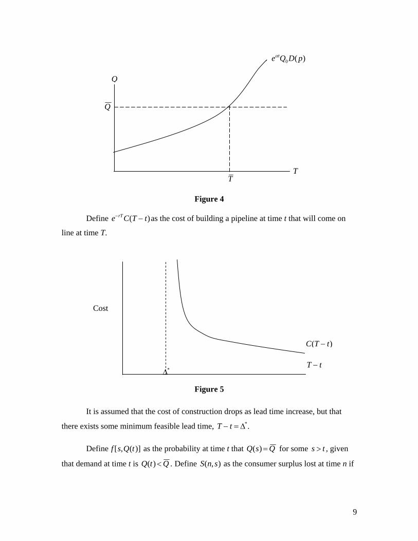
Figure 1

Pipelines have a high fixed cost, and for a substantial portion of their operating

region low marginal costs. The capacity of the pipeline is ultimately limited by the

pressure limits of pipe. Figure 1 illustrates the cost curves for a 48-inch pipeline 100

miles long. At a pressure limit of 1,500 pounds per square inch, the pipeline reached its

limit at approximately 3,800 million cubic feet per day. The dashed line denotes this

limit. At this point it becomes impossible to increase throughput by increasing power

and it becomes necessary to add compressor stations that increases throughput without

exceeding the line limit by increasing the pressure gradient. Note that this formulation

leads to a cost of moving 1 MCF of gas 1000 miles to be $.50.

5

We have shown in an earlier paper (Brito and Rosellon (2002) that the netback-

pricing rule is the solution of a static welfare optimization problem if the fee for

transporting gas is the marginal cost of transporting gas. However, marginal cost pricing

results in a loss or rents. (See Figure 1.) One solution to this problem is to set a fee that

yields a regulated rate of return over the life of the project sufficient to cover all costs. An

alternative, more sophisticated alternative is a two-part tariff with a price cap. The

sophisticated price cap mechanism is efficient in that it sets the marginal cost of

transporting gas equal to the variable change for moving gas. The question is whether the

more efficient allocation of resources merits the additional difficulties in regulation.

Dp()

p

Q

MC

AC

Figure 2

The shaded area in Figure 2 illustrates the welfare loss associated with using

average cost rather than marginal cost in transporting gas. The loss, L, is given by

6

(3) L =AC − MC( )2Qη

2p

where η is the elasticity of the demand for gas. Simple calculations suggest that for

elasticities in the demand for gas in the range of - 0.1 to - 0.2 the welfare loss is of second

order and can be ignored. If we calculate the dead weight loss for 4 million MCF the

price of gas equal to $2.00 per 1,000 cubic feet, an elasticity for the demand for gas equal

to -0.1, and a differential between AC and MC of $0.02, we get that the change in

demand is 4,000,000 cubic feet and the deadweight loss is $40. Since the cost of moving

gas is linear with distance, the deadweight loss over a distance of 1000 miles is $400 for

4 million MCF of gas. At a price of $4.00 per MCF, the welfare loss would be half.

The welfare loss associated with using a rate of return fee structure for transport

pipelines is so small that it is hard to see how the additional complexity in regulation can

be justified given the low elasticity in the demand for gas in Mexico.

The low elasticity of the demand for gas has some implications on the

implementation of the netback rule for pricing natural gas. The net back rule leads to the

optimal price of gas in that the price of gas is the opportunity cost of gas. However, the

price of gas is very sensitive to small in the geographical demand for gas. Since demand

for gas tends to be concentrated at mass point along the pipeline system, a very small

change in demand can result in a substantial change in the price of gas. Initially this was

not an issue of policy concern. Gas from the southern fields was reaching Los Ramones.

However, as of late, the demand for gas in the south of Mexico has increased to the point

where the physical arbitration point is at Cempoala in the south of Mexico. There is

pressure on the CRE to move the point used to price gas south to Cempoala.

In a first best world there is no question that Cempoala is the correct point to price

gas. The opportunity cost of gas to Mexico is the price of gas in Houston corrected fro

transport cost. There are two separate independent arguments that can be made against

moving the arbitration point to Cempoala. First is that it is not a first best world and, in

theory, there exist incentives for Pemex to invest and produce so as to move the

7

arbitration point south. Whether they do so or not is not a question we cannot answer. As

economists all we can say is that the incentives to manipulate the price of gas exist. (See

Brito and Rosellon 2003).

The second reason is political. Because the demand for gas is so inelastic, pricing

gas in Mexico is essentially a question of the redistribution of rents. For example, moving

the arbitration point by 500 miles will cause the price of gas to change by $.50 per MCF.

At a price of $3.50 per MCF the distortion cause by a subsidy is one-third cent per MCF.

(See Figure _3__ below). Given the other distortions in the economy, a distortion that

small is simply not large enough to argue that economic considerations should trump

political considerations in the setting of the arbitrage. Using Houston as a benchmark to

price gas is a useful instrument in deciding whether to use natural gas to produce

ammonia nitrate; it is not a particularly useful tool in allocating the use of gas between

Monterrey and Puebla.

Consider the following example. Suppose the arbitration points were at Los

Ramones and 10 MCF a day of gas was reaching Los Ramones from the southern fields.

Now a tortillería that consumes 20 MCF of gas a day moves form Monterrey to Puebla.

The arbitration point is now at Cempoala. Does it make sense to change the entire pricing

structure of gas in central Mexico because a tortillería has moved from Monterrey to

Puebela?

8

$0.000

$0.001

$0.002

$0.003

$0.004

$0.005

$0.006

$0.007

$0.008

$0.009

$0.010

$0.00 $1.00 $2.00 $3.00 $4.00 $5.00 $6.00 $7.00 $8.00 $9.00 $10.00

Price of Gas

Figure 3

3. Timing of Investment in Pipeline Capacity: The General Case

Let us consider the case when gas is being transmitted a distance L over a pipeline

of diameter D. The demand for gas is given by

(4) Q(t) = eαtQ0D(p)

where α is a random variable with mean α and p is a random variable with mean p .

Some of the stochastic elements are short term such as weather and others are long term

that can reflect macroeconomic conditions tine Mexico and in the United States.

The pressure limit on the pipeline is Q and we will define T such that

Q = eα T Q0D(p ).

9

Figure 4

Define e−rTC(T − t)as the cost of building a pipeline at time t that will come on

line at time T.

Figure 5

It is assumed that the cost of construction drops as lead time increase, but that

there exists some minimum feasible lead time, T − t = ∆*.

Define f [s,Q(t)] as the probability at time t that Q(s) = Q for some s > t , given

that demand at time t is Q(t) < Q . Define S(n, s) as the consumer surplus lost at time n if

∆*

Cost

C(T − t)

T − t

eαtQ0D( p)

Q

Q

T T

10

the constraint the constraint becomes binding at time s. The welfare loss, W (s) of the

constraint binding at time s is thus,

(5) W (s) = S(n, s)dss

T

∫

and the expected welfare lost at time t is:

(6) E[W (t)] = f [s,Q(t)] S(n, s)dndss

T

∫t

T

∫

If the constraint binds, the price of gas will have to increase as gas cannot move to

equilibrate the market at the netback price.

Figure 6

Define R(s,n)as the rents at time n if the constraint becomes binding at time s.

Define the total transfer that results from these rents as Z(s). Thus, if the constraint

binding at time s,

pn

Q

pc

D(p)

S(p)

Q

11

(7) Z(s) = R(s,n)dns

T

∫

and the expected value of transfers at time t is:

(8) E[Z(t)] = f [s,Q(t)] R(s,n)dndss

T

∫t

T

∫

These are transfer from the consumers of gas to Pemex and as such they do not

represent a loss in welfare. The fact that they have chosen not to do so suggests that in

some political or economic calculation that is more general than the timing of investment

in pipelines it was decided that the benefits from taxing gas were out weighed by other

economic or political factors.

Strictly speaking, the calculation of the optimal timing of pipeline investment

should be done in the context of the more general problem. This is not possible, but we

can approximate the more general problem by assigning a cost α to the transfers so that

the cost of the transfers is given by

(9) E[X(t)] = αE[Z(t)], 0 ≤ α ≤1

where α = 0 means that there is no cost to the government associated with transfers cause

by congestion of the pipelines and α =1 means that the interests of the government and

the consumers of gas are identical.

We can then compare the outcome of this maximization with policies that are

Pareto superior under the assumption that the government does not want to tax gas by

collecting the transfers caused congestion. That is to say, we can assume the government

does not want this revenue since they could have collected it by taxation and chose not to

do so. Then, if gas consumers are willing to pay for a level of pipeline capacity that

12

eliminates transfers, then they are better off and no one is worst off. Such a policy would

be Pareto superior to one that could result in congestion and transfers.

4. Optimal Investment in Pipeline

Let us assume that Pemex is trying to time investment in gas pipelines to

minimize a cost function that is the sum of the investment in pipelines, loss of consumer

surplus and a weight sum of the transfers:

(10) Y(t) = e−rTC(T − t) + f [s,Q(t)] S(n,s)dndss

T

∫t

T

∫ + α f [s,Q(t)] R(s,n)dndss

T

∫t

T

∫

this expression can be written as

(11) Y(t) = e−rTC(T − t) + f [s,Q(t)] [S(n,s) + αR(s,n)]dndss

T

∫t

T

∫

If we differentiate with respect to T, we get

(12)

dY(t)dT

= e−rT [∂C(T − t)∂T

− rC(T − t)] + f [T,Q(t)] [S(n,s) + αR(s,n)T

T

∫ ]dn

+ f [s,Q(t)][S(t,s) + αR(t,n)t

T

∫ ]ds

The term f [T,Q(t)] [S(n,s) + αR(s,n)T

T

∫ ]dn = 0 so

(13) dY(t)dT

= e−rT [∂C(T − t)∂T

− rC(T − t)] + f [s,Q(t)][S(t,s) + αR(t,n)t

T

∫ ]ds

and we get the expected result that the target date of completion of the pipeline is when

expected marginal benefits are equal to the marginal cost. There are two problems. First,

13

the distribution function on the probability that the constraint will be binding is not well

defined and depends on such factors as the performance of the United States economy.

Second, the solution depends on the subjective value of the parameter α . The outcome is

substantially a function of the choice of α . If we assume that the demand function is

locally linear then

(14) ∆p =∆QpηQ

and

(15) S(s,n) =∆p∆Q

2

and

(16) R(s,n) = ∆pQ

so ratio

(17) ρ =∆pQ

∆p∆Q2

=2Q ∆Q

=2

eα ( t−T ) −1≈

2α (t − T )

If we assume α = .06 and T − t =1

12, then α (t − T ) = .005 and ρ = 400. Note, however,

that the solution depends on the value of α which is subjective.

5. Timing of Investment in Pipeline Capacity: An Alternate Approach

14

Let us again consider the case when gas is being transmitted a distance L over a

pipe line of diameter D. The demand for gas is given by

(18) Q(t) = eαtQ0D(p)

where α is a random variable with mean α and p is a random variable with mean p . The

pressure limit on the pipeline is Q and we will define T such that Q = eα T Q0D(p ).

Assume that initial demand is given by Q 2

so the expect time for the pipeline to

reach full capacity is t = ln(2)α

Now let us consider a sequence of investment such that

pipeline capacity is doubled every time the pipeline reaches full capacity. Thus there is a

sequence of investments at Ti, where Ti = Ti−1 + t . Let c1 be the charge for transporting

gas. The present value of the revenues of the pipeline are given by

(19) PV1 = e− irt

i= 0

∞

∑ Q 2

c10

t

∫ e(α −r)sds =c1Q

2(1− e−rt )((α − r)[1− e(α −r)t ](1− e−rt )

⎛

⎝ ⎜

⎞

⎠ ⎟

Now consider any other sequence of investment ˜ T i , where ˜ T i = ˜ T i−1 + ˜ t . and let c2 be

the charge for transporting gas. Then

(20) PV2 = e−ir˜ t

i=0

∞

∑ Q 2

c20

˜ t

∫ e(α −ir)sds =c2Q

2(α − r)[1− e(α −r ) ˜ t ](1− e−r˜ t )

⎛

⎝ ⎜

⎞

⎠ ⎟ .

If we assume the consumer of natural gas is paying for the buffer capacity, then

PV1 = PV2 and

15

(21) c1Q 2(1− e−rt )((α − r)

[1− e(α −r )t ](1− e−rt )

⎛

⎝ ⎜

⎞

⎠ ⎟ =

c2Q 2(α − r)

[1− e(α −r ) ˜ t ](1− e−r˜ t )

⎛

⎝ ⎜

⎞

⎠ ⎟

or

(22) c2

c1

=[1− e(α −r )t ](1− e−r˜ t )[1− e(α −r )˜ t ](1− e−rt )

and the difference in he costs can be expressed as a function of c1,

(23) c2 − c1 =[1− e(α −r)t ](1− e−r˜ t )[1− e(α −r)˜ t ](1− e−rt )

−1⎛

⎝ ⎜

⎞

⎠ ⎟ c1.

The cost per thousand cubic feet of gas transported for maintaining a t − ˜ t buffer of

excess capacity, ∆C is given by substituting into equations (19) and (20).

(24)∆C = c1 e−rt

0

t

∫ [1− e(α −r)t ](1− e−r˜ t )[1− e(α −r)˜ t ](1− e−rt )

−1⎛

⎝ ⎜

⎞

⎠ ⎟ dt =

1r

[1− e(α −r)t ](1− e−r˜ t )[1− e(α −r)˜ t ](1− e−rt )

−1⎛

⎝ ⎜

⎞

⎠ ⎟ (1− e−r˜ t )c1

Let us calculate a simple example assuming that r = .12 and α = .06 , and that the

cost without a buffer is $.10 per 1000 cubic feet. If there is no buffer then at a growth rate

of six percent a year, t =11.5. Table 1 below gives the cost per MCF of maintaining

excess buffer capacity.

Cost per Year of Pipeline Buffer Capacity Year Change in Tariff

dollars Present Value of Cost

dollars 1 .006 9.37 2 .013 19.32 3 .020 29.12 4 .027 41.12 5 .035 53.04

Table 1

16

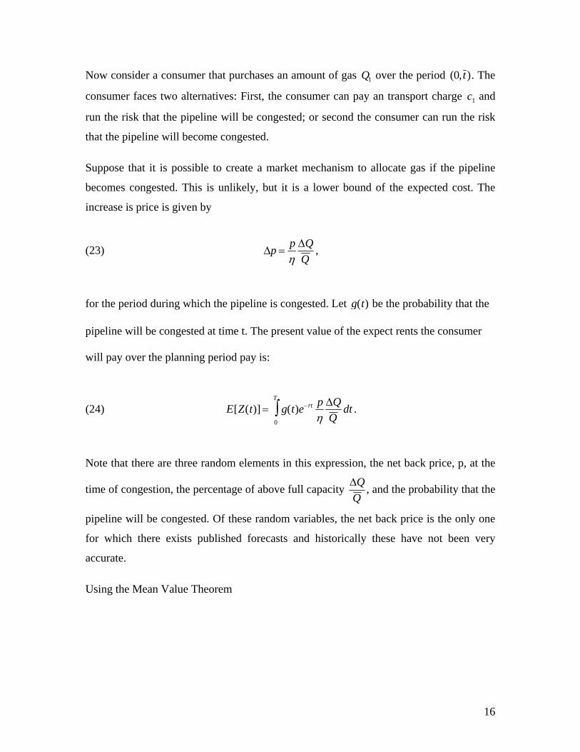
Now consider a consumer that purchases an amount of gas Q1 over the period (0, t ). The

consumer faces two alternatives: First, the consumer can pay an transport charge c1 and

run the risk that the pipeline will be congested; or second the consumer can run the risk

that the pipeline will become congested.

Suppose that it is possible to create a market mechanism to allocate gas if the pipeline

becomes congested. This is unlikely, but it is a lower bound of the expected cost. The

increase is price is given by

(23) ∆p =pη

∆QQ

,

for the period during which the pipeline is congested. Let g(t) be the probability that the

pipeline will be congested at time t. The present value of the expect rents the consumer

will pay over the planning period pay is:

(24) E[Z(t)] = g(t)e−rt

0

T

∫ pη

∆QQ

dt .

Note that there are three random elements in this expression, the net back price, p, at the

time of congestion, the percentage of above full capacity ∆QQ

, and the probability that the

pipeline will be congested. Of these random variables, the net back price is the only one

for which there exists published forecasts and historically these have not been very

accurate.

Using the Mean Value Theorem

17

(25) g(t)e−rt

0

t

∫ pη

∆QQ

dt =ˆ p η

∆ ˆ Q Q

g(t)e−rt

0

t

∫ dt > e−rt ˆ p η

∆ ˆ Q Q

t

Since we are evaluating the integral at the end point, T. The expression, e−rT ˆ p η

∆ ˆ Q Q

T , is a

lower bound of the expected cost of congestion to the consumer. If we assume that

consumers are risk neutral, we can construct a variable such that

(26) e−rT ˆ p η

∆ ˆ Q Q

T = e−rT ˆ p η

∆ ˆ Q Q

πt = e−rT ˆ p η

θt

In this formulation, θ =∆ ˆ Q Q

π is the expected over capacity and t is the number of days

the pipeline is congested. Thus we an express a lower bound of the tradeoff for

consumers between buffer capacity to the pipeline and days of expected over capacity for

a given value of θ .

(27) e−rt ˆ p η

θt =1r

[1− e(α −r )t ](1− e−r˜ t )[1− e(α −r )˜ t ](1− e−rt )

−1⎛

⎝ ⎜

⎞

⎠ ⎟ (1− e−r˜ t )c1

which can be solved for t.

(28) t =ert ηθˆ p r

[1− e(α −r) t ](1− e−r˜ t )[1− e(α −r) ˜ t ](1− e−rt )

−1}⎛

⎝ ⎜

⎞

⎠ ⎟ (1− e−r˜ t )c1

Figure A below gives the relationship for a price of gas of $3.00 per MCF. To

illustrate, an individual whose subjective expectation is that θ = .04 would rather pay the

costs associated with two years of excess capacity rather than risk 31.6 days of

18

congestion. An individual whose subjective expectation is that θ = .12 would rather pay

the costs associated with two years of excess capacity rather than risk 10.6 days of

congestion.

Price of Gas $3.00 MCF

10

15

20

25

30

35

2 3 4

Years of Buffer Capacity

1

.12

.10

.04

.08

.06

5

Figure 7

Similar calculations can be performed for other assumptions about the price of

gas. Alternatively, it is possible to examine the relationship between days of congestion

and the price of gas for a fixed amount of amount of buffer. This is illustrated in Figure

B. Suppose the price of gas is expected to be in the range of $3.00 to $6.00, then

individuals whose subjective expectation of θ was greater than .04 would rather pay for

two years of excess capacity rather than risk 30 days of congestion.

19

0

5

10

15

20

25

30

35

40

45

50

0 1 2 3 4 5 6 7 8

.04

.12

Max & Min for Two Year Buffer

Price of Gas

Figure 8

An Example 2-24-

To get an intuitive insight as to what could lead to 30 days of congestion, it is

useful to compute a simple example. Assume that a pipeline has an increase of

throughput that grows at six percent a year. If initial throughput is Q 2

where the capacity

of the pipeline is Q we can expect the pipeline to be congested in 11.5 years. Now

suppose that after 9.5 years the growth rate increased by a one percent so that α = .07.

The question is how days of congestion will result at θ = .04 ? The quick answer is 34. If

Days of Congestion

20

throughput is growing at a rate α = .06, then after 8.5 years throughput will be equal to

1.67Q 2

. At a growth rate of .07 after the ninth year the pipeline will reach capacity after

11.12 years. The number of days of congestion at θ = .04 is

Tc =(e.07t

0

.43

∫ −1)dt

.04 × .43= 34.

The numerator is the cumulative θ and the dominator normalizes it for θ = .04 .

Using very naïve calculations, a growth rate of .07 rather than .06 in the last three years

of the planning period would result in over 30 days of congestion. The real world is very

much more complicated and there are problems such as construction delays, weather,

macro-economic shocks, or war in the Middle East. The cost of buffer capacity is low

and the cost of transfers that result from congestion to the consumers of gas of congestion

is very high.

This completely ignores social and political costs that would result if the gas

pipeline system becomes congested and gas cannot flow to clear the market.

6. Conclusions

The fact that the demand for gas is very inelastic in Mexico is a two edged sword

with respect to the administration of the net back rule for pricing gas. On one hand, a

very small change in the demand for gas can lead to a large change in the arbitration

point, however on the other hand the fact that the demand for gas is very inelastic means

that the welfare loss associated with the pricing of gas based on an artificial pricing point

is very small. Cempoala is about 500 miles from Los Ramones so a shift of the arbitrage

point from Los Ramones to Cempoala would lead to a change in the price of gas of

approximately $.50 per MCF. However at a price of $3.50 per MCF the welfare loss

associated keeping the arbitrage point at Los Ramones is on the order of one third cent

per MCF. Since very small changes in the demand for gas can lead to substantial changes

in the net back price and since the welfare losses from maintaining an artificial point for

price are low, the question is more political than economic. The opportunity cost of gas

21

based on the Houston market can be used to argue why natural gas in Mexico should not

be used to produce ammonia nitrate. It is harder to use that price to justify why a factory

in Puebla should pay substantially more for gas than a factory in Monterrey. As

illustrated in the example of the tortillería, this is particularly true when a very small

change in the pattern of demand can lead to a substantial change in the price of gas. The

fact that the demand for gas is very inelastic means that the welfare cost of keeping price

of gas stable in Mexico is low.

Similarly, the fact that the demand for gas is very inelastic in Mexico is a two

edged sword with respect to pipeline capacity. A ten percent increase in demand would

result in a one hundred percent increase in the price that would clear the market is gas is

not free to flow to maintain the net back price. However the fact that the demand is so

inelastic permits the implementation of a very simple rate structure and appears to justify

investment in substantial buffer capacity. Such capacity may be Pareto superior.

Substantiation of the latter conjecture is beyond the limited scope of this paper. However,

calculations suggest that users would prefer to pay for excess capacity in the pipeline

system than to risk the consequences of congestion. Since the parameters needed to

calculate this result are subject, it must remain a conjecture. Experience in the United

States suggests that such periods of congestion do occur. The price of gas in the United

States is set by market forces and an equilibrium can be reached. The netback rule,

however, requires that gas be able to flow to achieve equilibrium.

References Adelman, M.A, 1963, The Supply and Price of Natural Gas, (B. Blackwell, Oxford). Brito, D. L., W. L. Littlejohn and J. Rosellón, 2000, “Pricing Liquid Petroleum Gas in

Mexico, Southern Economic Journal, 66 (3), 742-753. Brito, D. L. and J. Rosellón, 2003, “Strategic Behavior and Pricing of Gas,” manuscript. Brito, D. L. and J. Rosellón, 2002, “Pricing Natural Gas in Mexico: an Application of the

Little-Mirrlees Rule,” The Energy Journal, 23 (3), 81-93. Comisión Reguladora de Energía, 1996, "Directiva sobre la Determinacion de Precios y

Tarifas para las Actividades Reguladdas en materia de Gas Natural," MEXICO. (WEB SITE:http://www.cre.gob.mx)

22

Little, I. M. D. and J.A. Mirrlees, 1968, Manual of Industrial Project Analysis in

Developing Countries, (Development Centre of the Organization for Economic Co-Operation and Development, Paris)

Pemex, 1998, “Indicadores Petroleros y Anuario Estadístico”. Rosellon, J. and J. Halpern, 2001, “Regulatory Reform in Mexico’s Natural Gas Industry:

Liberalization in Context of Dominant Upstream Incumbent,” Policy Research Working Paper 2537, The World Bank.

Secretaría de Energía, 1998, “Prospectiva del Mercado de Gas Natural, 1998-2007.”

(WEB SITE:http://www.energia.gob.mx/frame4.html)