S. L. Davis, M. D. Dukes A Tribute to the Career of
Terry Howell, Sr.
ABSTRACT. In unincorporated Orange County, Florida, 57% to 62% of single-family residential homes were found to regularly over-irrigate, resulting in the need to find better ways to schedule automatic irrigation. The objective of this research was to evaluate the effects of programming for identical virtual landscapes to further explore the water savings potential of evapotranspiration (ET) controllers. As a virtual test, three Rain Bird ET controllers were studied: the ESP-SMT controller with two firmware options (original and an updated), and the ESP-SMTe, a replacement product for the ESP-SMT. Irrigation was scheduled for a virtual central Florida landscape by altering possible program settings of plant type, microclimate, soil type, and density that relate directly to parameters used in the soil water balance. The ESP-SMTe consistently applied similar amounts of irrigation to the ESP-SMT with updated firmware, indicating that controller updates were minor between the two models. The settings were optimized for Florida landscapes by selecting a heavier soil type, increasing the shade, and selecting a medium stand for a custom plant type, resulting in reductions in irrigation application. The ESP-SMTe and ESP-SMT with updated firmware were different from the ESP-SMT with original firmware, where newer models applied more water despite identical settings, averaging 12 to 21 mm more per month than the original firmware. Additionally, all of the controllers were unable to fully account for rainfall throughout the test resulting in a minimum of 51% in over-irrigation compared to the gross irrigation requirement (GIR). Increasing the accuracy of rainfall accounting would be extremely beneficial to overall water conservation and efficiency. In a separate, independent ET controller study, there was a large discrepancy in irrigation application among multiple brands programmed to irrigate the same virtual landscape. This further shows the importance of understanding the algorithms behind the program settings.
lorida is currently ranked as the third most populous state with an average increase in population of 803 new residents per day, estimated from July 2013 to July 2014 (U.S. Census Bureau,
2014). Central Florida continues to be faced with positive population growth combined with limitations to available groundwater resources. When increasing pumping capacity to address population growth is not an option, increasing water conservation and efficiency becomes a top priority of utilities.
Targeting efficiency in automatic irrigation has become increasingly important with estimates of over half of total
household water use going toward landscape irrigation (Haley et al., 2007; Devitt et al., 2008). Specifically for Orange County Utilities (unincorporated Orange County, Fla.), 57% to 62% of single-family residential homes were regularly over-irrigating compared to calculated landscape irrigation requirements (Romero and Dukes, 2014). Finding better ways to schedule automatic irrigation has become a high priority as the installation of automatic irrigation systems continues to be standard practice.
A technological method for scheduling irrigation is a smart controller that can adjust or override irrigation based on weather or soil conditions (Dukes, 2012). Currently, there are two commercially-available products designated as smart controllers. Weather-based irrigation controllers, or evapotranspiration (ET) controllers, typically use weather information, user-selected program settings, and proprietary algorithms to determine the irrigation schedule instead of relying on manually selected runtimes. Soil moisture sensor (SMS) controllers bypass irrigation events when the measured soil moisture is greater than a user set threshold. More detailed descriptions of smart controller functionality and performance can be found in Davis et al. (2009), McCready et al. (2009), Davis and Dukes (2010), McCready and Dukes (2010), and Cardenas-Lailhacar and Dukes (2012).
Submitted for review in January 2015 as manuscript number NRES
11182; approved for publication by the Natural Resources &Environmental Systems Community of ASABE in January 2016. Presented at the 2014 ASABE Annual Meeting as Paper No. 2144234.
The authors are Stacia L. Davis, ASABE Member, Assistant Professor, Louisiana State University Agricultural Center, Bossier City,Louisiana; and Michael D. Dukes, ASABE Member, Professor,Agricultural and Biological Engineering, Director, Center for LandscapeConservation & Ecology, Institute of Food and Agricultural Sciences,University of Florida, Gainesville, Florida. Corresponding author: StaciaL. Davis, Assistant Professor, Louisiana State University AgriculturalCenter, Red River Research Station, 262 Research Station Drive, BossierCity, LA, 71112-9638; phone: 318-741-7430; e-mail: [email protected].
F
252 APPLIED ENGINEERING IN AGRICULTURE
To address the growing public water demands in Orange County, a study was conducted to determine the water conservation potential of smart controllers implemented on residential landscapes of excessive irrigators (Davis and Dukes, 2015a; 2015b). All single-family homes within the Orange County Utilities service area were evaluated for over-irrigation tendencies by comparing estimated irrigation application from billing data and parcel information to the calculated gross irrigation requirement (GIR) as a monthly landscape irrigation ratio (LIR) using the methods described in Romero and Dukes (2014). Once the 167 participants were selected for the study, they were re-evaluated with site-specific information and were found to have excessive irrigation patterns, averaging 6 to 8 times the GIR (Davis and Dukes, 2015a), thus confirming the methodology for selecting high outdoor water users.
A portion of the Orange County smart controller study (Davis and Dukes, 2015a; 2015b) focuses on differences in irrigation application based on the program settings supplied to the ET controllers by the contractor or recommended optimized settings based on previous UF-IFAS work. Davis and Dukes (2015b) showed that the ET controller with contractor settings typically applied less irrigation per week than the comparison group with no smart technology, depending on season. An additional decrease in average weekly irrigation application resulted when the ET controller was programmed with optimized settings. However, it is unclear how the differences in these program settings helped to reduce irrigation application. The objective of this research was to evaluate the effects of irrigation application by changing ET controller program selections for identical virtual landscapes as a way to further explore their water savings potential.
MATERIALS AND METHODS A total of three independent studies were conducted as a
part of this evaluation: (a) central Florida smart controller study, (b) virtual test of Rain Bird ET controllers, and (c) independent virtual test of multiple brands. The central Florida smart controller study, as was discussed in the introduction and in Davis and Dukes (2015a; 2015b), was a field study conducted in Orange County, Florida, with single-family homes using smart technologies. The virtual test of Rain Bird ET controllers was conducted as a portion of the field study to further evaluate program settings of the controllers (and is the focus of this article). The independent virtual test of multiple brands was conducted as part of a completely separate study conducted in conjunction with a manufacturer to evaluate product brands irrigating a single virtual landscape scenario.
VIRTUAL TEST OF RAIN BIRD ET CONTROLLERS In a virtual test, four ET controllers were installed at an
outdoor testing site located on the University of Florida main campus in Gainesville, Florida (fig. 1). Three controllers were the ESP-SMT (Rain Bird Corporation, Azusa, Calif.) and one controller was the ESP-SMTe (Rain Bird Corporation, Azusa, Calif.); all controllers and
program selections were chosen to represent variations of the treatments implemented in the central Florida smart controller study (Davis and Dukes, 2014a; 2015b) (fig. 2).
Two ESP-SMT controllers were installed with factory-packaged components thus utilizing the original version of firmware (2009-2010). It was found in Davis et al. (2009) that replications of ET controllers of the same model, and firmware, had identical performance since the scheduling algorithms are identical. The third ESP-SMT was installed with a panel that utilized updated firmware released in 2011.
The ESP-SMTe is the current model of ET controller offered by the Rain Bird Corporation. Some of the product features of both the ESP-SMT and ESP-SMTe are available in product literature, including a few of the differences between the models, but most algorithms are proprietary and unknown. The most obvious differences were the removal of density selections when the plant type is a turfgrass material, slight modifications to crop coefficient values, and the removal of efficiency factors.
Figure 1. Four Rain Bird ET controllers were installed on the University of Florida campus located at the corner of Hull Road (south) and Museum Road (west).
Figure 2. Three ESP-SMT and one ESP-SMTe were programmed to schedule irrigation for multiple configurations of landscape settings possible in central Florida. Each controller had an independent rain gauge (fourth gauge not pictured).
32(2): 251-262 253
A total of 28 zones were programmed on the three ESP-SMT controllers with 15 zones using the original firmware and 13 zones using the updated firmware (tables 1-2). The ESP-SMTe was programmed with 18 zones that replicated settings of zones on the ESP-SMT for direct comparison (table 3). Program settings for each zone varied by a single variable to determine the effect of monthly irrigation application as a result of that variable. Variables included plant type, microclimate, soil type, and density.
The controllers were installed in an outdoor location to maintain proper functionality of the weather-based devices, such as taking accurate measurements of temperature and rainfall, but they were not associated with physical irrigation systems or turfgrass plots. Instead, all 46 zones were wired to a series of circuit panels connected to a field laptop personal computer running an executable program coded in Visual Basic (fig. 3). When a zone was activated by the controller, a timestamp was generated to signify the start of the electrical signal. Another timestamp occurred when the electrical signal disappeared, indicating that the zone deactivated. Accuracy of the timestamps fell within two seconds. The timestamp data was output to a text file that was periodically downloaded from the computer.
Manual irrigation data was transcribed from all four controllers during the study period to verify results provided by the data logging system. Gross irrigation was calculated from the timestamps using the application rates programmed for the corresponding zones.
As a comparison, the gross irrigation requirement (GIR) was calculated to provide an estimate of theoretical irrigation needs using a soil water balance, similar to the functionality of an ET controller. In a virtual test such as this, there are no measured irrigation depths for comparison; thus, the GIR was considered to be a benchmark for evaluating ET controller performance. The GIR was calculated by multiplying the net irrigation water requirement (IWRnet) by an efficiency factor, which was identical to the value programmed into the controllers. The IWRnet is the amount of irrigation required to replenish available water holding capacity (AWC) of the soil, or the maximum depth of water that can be stored after gravitational drainage (Irrigation Association, 2005). The IWRnet was determined from mass conservation of soil water content (Irrigation Association, 2005):
IWRnet = PWR − Re (1)
Table 1. Program settings for zones running on the Rain Bird ESP-SMT controllers with the original firmware.
Panel[a] Zone Application Rate
(mm/h) Efficiency Crop Coefficient
(KC) Root Zone
(mm) Microclimate Soil Type Density A 1 41 1 0.6 203 25% Shade Loamy Sand Dense A 2 41 1 0.6 203 25% Shade Sandy Loam Dense A 3 41 0.65 WT[b] 76 Full Sun Sand Dense A 4 41 0.65 WT 76 Full Sun Loamy Sand Dense A 5 41 0.65 0.6 203 25% Shade Loamy Sand Dense A 6 41 0.65 0.6 203 Full Sun Loamy Sand Dense A 7 41 1 0.6 203 25% Shade Loamy Sand Medium A 8 41 1 0.6 203 25% Shade Sand Dense B 1 41 0.65 CT[c] 76 Full Sun Loamy Sand Dense B 2 41 0.65 CT 76 Full Sun Sand Dense B 3 41 0.65 WT 76 Full Sun Loamy Sand Medium B 4 41 1 0.6 203 25% Shade Loam Dense B 5 41 1 0.6 203 50% Shade Loamy Sand Dense B 6 41 1 0.6 203 75% Shade Loamy Sand Dense B 7 41 1 0.6 203 Full Sun Loamy Sand Dense
[a] Two controllers having the same firmware were used to program all 15 zones. [b] WT represents warm season turfgrass as the plant type settings with crop coefficients selected for Bermudagrass in the SWAT testing protocol
(Irrigation Association, 2008). [c] CT represents cool season turfgrass as the plant type settings with crop coefficients selected for Tall Fescue in the SWAT testing protocol (Irrigation
Association, 2008).
Table 2. Program settings for zones running on the Rain Bird ESP-SMT controller with the updated firmware.
Zone Application Rate
(mm/h) Efficiency Crop Coefficient
(KC) Root Zone
(mm) Microclimate Soil Type Density 1 41 1 WT[a] 76 Full Sun Sand Medium 2 11 1 WT 76 Full Sun Sand Medium 3 41 1 CT[b] 76 Full Sun Sand Medium 4 41 1 WT 76 Full Sun Loamy Sand Medium 5 41 1 WT 76 Full Sun Sandy Loam Medium 6 41 1 WT 76 25% Shade Loamy Sand Medium 7 41 1 WT 76 50% Shade Loamy Sand Medium 8 41 1 WT 76 75% Shade Loamy Sand Medium 9 41 1 0.6 203 25% Shade Loamy Sand Dense 10 41 1 0.6 203 25% Shade Loamy Sand Medium 11 41 1 0.6 203 Full Sun Sand Medium 12 41 1 WT 76 Full Sun Loam Medium 13 41 1 WT 76 Full Sun Sand Dense
[a] WT represents warm season turfgrass as the plant type settings with crop coefficients selected for Bermudagrass in the SWAT testing protocol (Irrigation Association, 2008).
[b] CT represents cool season turfgrass as the plant type settings with crop coefficients selected for Tall Fescue in the SWAT testing protocol (IrrigationAssociation, 2008).
254 APPLIED ENGINEERING IN AGRICULTURE
The PWR is the plant water requirement (mm) and Re is effective rainfall (mm). The IWRnet was accumulated daily, but was applied only when the soil water level fell below management allowable depletion (MAD), calculated as 50% of AWC (Irrigation Association, 2005). The AWC was selected to represent the two main soil types in Orange County, 43 mm for flatwoods soils, characterized as poorly to moderately drained sands, and 24 mm for uplands soils, characterized as excessively to moderately drained sands, based on a root zone depth of 305 mm for turfgrass (Davis and Dukes, 2015a). Deep percolation and surface runoff can be considered negligible with proper design and management of the irrigation system. Since this was a virtual test, it was assumed that the irrigation system would have been designed and maintained properly thus avoiding the need for estimating the parameters.
The PWR is the amount of water necessary to maintain healthy plant material (Irrigation Association, 2005) and was calculated as the plant-specific evapotranspiration (ETC) by taking into account plant characteristics using coefficients specific to the crop (KC), microclimate (KMC), and density (KD).
PWR = KC * KMC * KD * ETO (2)
Reference evapotranspiration (ETO) is the estimated evapotranspiration of a short reference crop assumed to be a dense, well-watered, cool-season turfgrass maintained at a 0.12 m height. The ETO was calculated by the American Society of Civil Engineers – Environmental and Water Resources Institute (ASCE-EWRI) standardized ET equation (ASCE, 2005). This equation used temperature, relative humidity, solar radiation, and wind speed collected from a weather station located on-site and maintained by the UF-IFAS research team from April 2012 through August 2013. Rainfall depths were also collected at this weather station. When data from this station was unavailable (Sept. 2013-Oct. 2014), the data was substituted from the weather station located 1.5 km away. As a comparison to the weather conditions during the study period, historical ETO and rainfall were estimated from 37 years of weather data collected from the National Weather Service weather station located at the Gainesville Regional Airport, approximately 10 km from the test site. Historical ETO was calculated using the ASCE-EWRI standardized ET equation.
The KC values are ratios of average ETC to average ETO. These values incorporate distinguishing characteristics of the specific crop to the reference crop such as crop height, crop-soil surface resistance, and albedo of the crop-soil surface (Allen, 2000). The KC values selected for these studies were updated monthly for warm season turfgrass located in central Florida with values of 0.45 (Dec.-Feb.), 0.60 (Nov.), 0.65 (Mar.), 0.70 (Jul., Aug., Oct.), 0.75 (Jun., Sep.), 0.80 (Apr.), and 0.90 (May) (Jia et al., 2009). For the
Table 3. Program settings for zones running on the Rain Bird ESP-SMTe controller.
Zone Application Rate
(mm/h) Efficiency Crop Coefficient
(KC) Root Zone
(mm) Microclimate Soil Type Density 1 41 1 WT[a] 76 Full Sun Sand NA[b] 2 11 1 WT 76 Full Sun Sand NA 3 41 1 CT[c] 76 Full Sun Sand NA 4 41 1 WT 76 Full Sun Loamy Sand NA 5 41 1 WT 76 Full Sun Sandy Loam NA 6 41 1 WT 76 25% Shade Loamy Sand NA 7 41 1 WT 76 50% Shade Loamy Sand NA 8 41 1 WT 76 75% Shade Loamy Sand NA 9 41 1 0.6 203 25% Shade Loamy Sand Dense 10 41 1 0.6 203 25% Shade Loamy Sand Medium 11 41 1 0.6 203 Full Sun Sand Medium 12 41 1 WT 76 Full Sun Loam NA 13 41 1 WT 76 Full Sun Sand NA 14 41 1 0.6 203 25% Shade Loamy Sand Medium 15 41 1 0.6 203 25% Shade Loamy Sand Medium 16 41 1 WT 203 25% Shade Loamy Sand NA 17 41 1 WT 203 25% Shade Loamy Sand NA 18 41 1 WT 203 25% Shade Loamy Sand NA
[a] WT represents warm season turfgrass as the plant type settings with crop coefficients selected for Bermudagrass in the SWAT testing protocol (Irrigation Association, 2008).
[b] Density is not an applicable setting when warm season turfgrass or cool season turfgrass settings are selected. [c] CT represents cool season turfgrass as the plant type settings with crop coefficients selected for Tall Fescue in the SWAT testing protocol (Irrigation
Association, 2008).
Figure 3. All four ET controllers were wired to circuit boardsconnected to a laptop running a Visual Basic program that recordstimestamps of irrigation events. This test was virtual, thus thecontrollers did not control physical irrigation systems.
32(2): 251-262 255
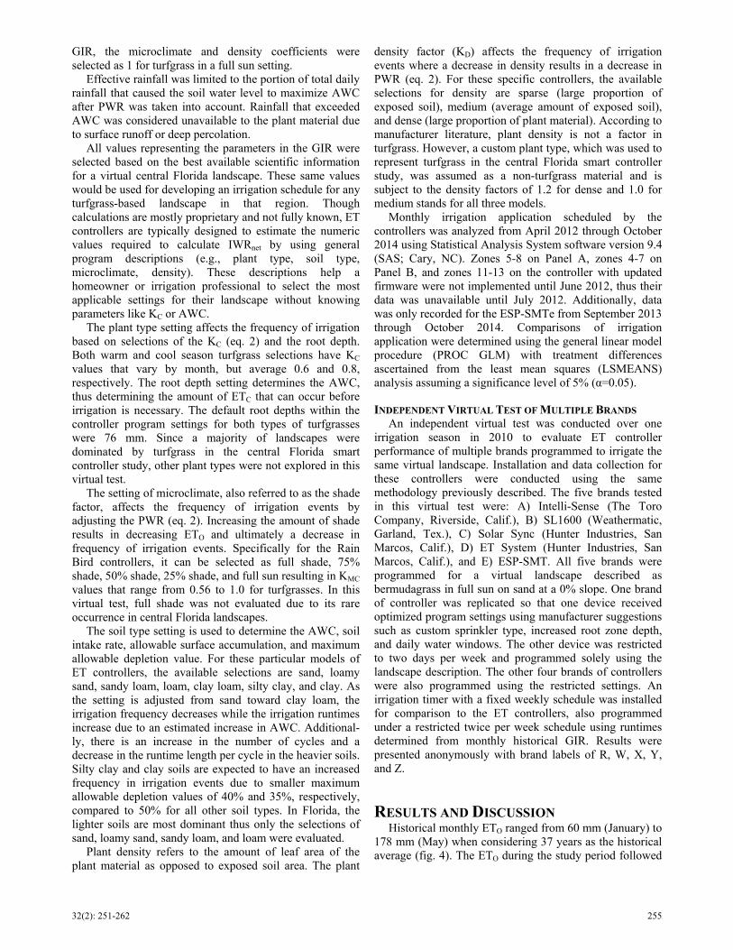
GIR, the microclimate and density coefficients were selected as 1 for turfgrass in a full sun setting.
Effective rainfall was limited to the portion of total daily rainfall that caused the soil water level to maximize AWC after PWR was taken into account. Rainfall that exceeded AWC was considered unavailable to the plant material due to surface runoff or deep percolation.
All values representing the parameters in the GIR were selected based on the best available scientific information for a virtual central Florida landscape. These same values would be used for developing an irrigation schedule for any turfgrass-based landscape in that region. Though calculations are mostly proprietary and not fully known, ET controllers are typically designed to estimate the numeric values required to calculate IWRnet by using general program descriptions (e.g., plant type, soil type, microclimate, density). These descriptions help a homeowner or irrigation professional to select the most applicable settings for their landscape without knowing parameters like KC or AWC.
The plant type setting affects the frequency of irrigation based on selections of the KC (eq. 2) and the root depth. Both warm and cool season turfgrass selections have KC values that vary by month, but average 0.6 and 0.8, respectively. The root depth setting determines the AWC, thus determining the amount of ETC that can occur before irrigation is necessary. The default root depths within the controller program settings for both types of turfgrasses were 76 mm. Since a majority of landscapes were dominated by turfgrass in the central Florida smart controller study, other plant types were not explored in this virtual test.
The setting of microclimate, also referred to as the shade factor, affects the frequency of irrigation events by adjusting the PWR (eq. 2). Increasing the amount of shade results in decreasing ETO and ultimately a decrease in frequency of irrigation events. Specifically for the Rain Bird controllers, it can be selected as full shade, 75% shade, 50% shade, 25% shade, and full sun resulting in KMC values that range from 0.56 to 1.0 for turfgrasses. In this virtual test, full shade was not evaluated due to its rare occurrence in central Florida landscapes.
The soil type setting is used to determine the AWC, soil intake rate, allowable surface accumulation, and maximum allowable depletion value. For these particular models of ET controllers, the available selections are sand, loamy sand, sandy loam, loam, clay loam, silty clay, and clay. As the setting is adjusted from sand toward clay loam, the irrigation frequency decreases while the irrigation runtimes increase due to an estimated increase in AWC. Additional-ly, there is an increase in the number of cycles and a decrease in the runtime length per cycle in the heavier soils. Silty clay and clay soils are expected to have an increased frequency in irrigation events due to smaller maximum allowable depletion values of 40% and 35%, respectively, compared to 50% for all other soil types. In Florida, the lighter soils are most dominant thus only the selections of sand, loamy sand, sandy loam, and loam were evaluated.
Plant density refers to the amount of leaf area of the plant material as opposed to exposed soil area. The plant
density factor (KD) affects the frequency of irrigation events where a decrease in density results in a decrease in PWR (eq. 2). For these specific controllers, the available selections for density are sparse (large proportion of exposed soil), medium (average amount of exposed soil), and dense (large proportion of plant material). According to manufacturer literature, plant density is not a factor in turfgrass. However, a custom plant type, which was used to represent turfgrass in the central Florida smart controller study, was assumed as a non-turfgrass material and is subject to the density factors of 1.2 for dense and 1.0 for medium stands for all three models.
Monthly irrigation application scheduled by the controllers was analyzed from April 2012 through October 2014 using Statistical Analysis System software version 9.4 (SAS; Cary, NC). Zones 5-8 on Panel A, zones 4-7 on Panel B, and zones 11-13 on the controller with updated firmware were not implemented until June 2012, thus their data was unavailable until July 2012. Additionally, data was only recorded for the ESP-SMTe from September 2013 through October 2014. Comparisons of irrigation application were determined using the general linear model procedure (PROC GLM) with treatment differences ascertained from the least mean squares (LSMEANS) analysis assuming a significance level of 5% (α=0.05).
INDEPENDENT VIRTUAL TEST OF MULTIPLE BRANDS An independent virtual test was conducted over one
irrigation season in 2010 to evaluate ET controller performance of multiple brands programmed to irrigate the same virtual landscape. Installation and data collection for these controllers were conducted using the same methodology previously described. The five brands tested in this virtual test were: A) Intelli-Sense (The Toro Company, Riverside, Calif.), B) SL1600 (Weathermatic, Garland, Tex.), C) Solar Sync (Hunter Industries, San Marcos, Calif.), D) ET System (Hunter Industries, San Marcos, Calif.), and E) ESP-SMT. All five brands were programmed for a virtual landscape described as bermudagrass in full sun on sand at a 0% slope. One brand of controller was replicated so that one device received optimized program settings using manufacturer suggestions such as custom sprinkler type, increased root zone depth, and daily water windows. The other device was restricted to two days per week and programmed solely using the landscape description. The other four brands of controllers were also programmed using the restricted settings. An irrigation timer with a fixed weekly schedule was installed for comparison to the ET controllers, also programmed under a restricted twice per week schedule using runtimes determined from monthly historical GIR. Results were presented anonymously with brand labels of R, W, X, Y, and Z.
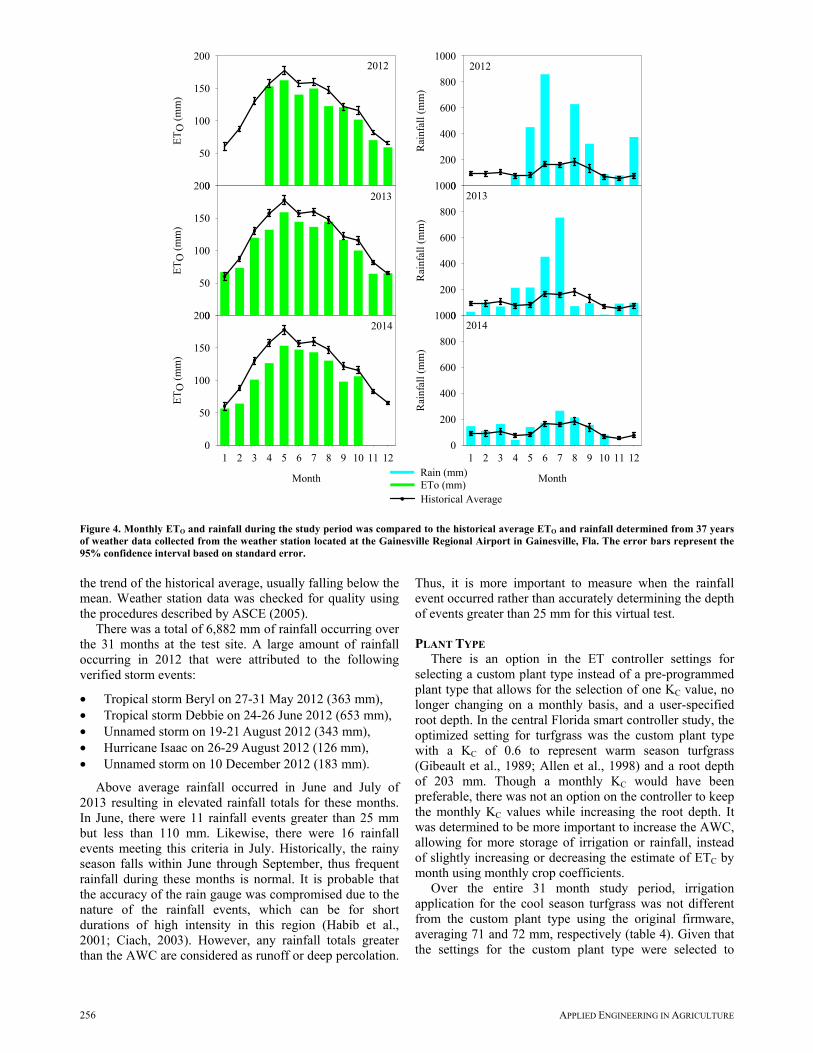
RESULTS AND DISCUSSION Historical monthly ETO ranged from 60 mm (January) to
178 mm (May) when considering 37 years as the historical average (fig. 4). The ETO during the study period followed
256 APPLIED ENGINEERING IN AGRICULTURE
the trend of the historical average, usually falling below the mean. Weather station data was checked for quality using the procedures described by ASCE (2005).
There was a total of 6,882 mm of rainfall occurring over the 31 months at the test site. A large amount of rainfall occurring in 2012 that were attributed to the following verified storm events:
• Tropical storm Beryl on 27-31 May 2012 (363 mm), • Tropical storm Debbie on 24-26 June 2012 (653 mm), • Unnamed storm on 19-21 August 2012 (343 mm), • Hurricane Isaac on 26-29 August 2012 (126 mm), • Unnamed storm on 10 December 2012 (183 mm).
Above average rainfall occurred in June and July of 2013 resulting in elevated rainfall totals for these months. In June, there were 11 rainfall events greater than 25 mm but less than 110 mm. Likewise, there were 16 rainfall events meeting this criteria in July. Historically, the rainy season falls within June through September, thus frequent rainfall during these months is normal. It is probable that the accuracy of the rain gauge was compromised due to the nature of the rainfall events, which can be for short durations of high intensity in this region (Habib et al., 2001; Ciach, 2003). However, any rainfall totals greater than the AWC are considered as runoff or deep percolation.
Thus, it is more important to measure when the rainfall event occurred rather than accurately determining the depth of events greater than 25 mm for this virtual test.
PLANT TYPE There is an option in the ET controller settings for
selecting a custom plant type instead of a pre-programmed plant type that allows for the selection of one KC value, no longer changing on a monthly basis, and a user-specified root depth. In the central Florida smart controller study, the optimized setting for turfgrass was the custom plant type with a KC of 0.6 to represent warm season turfgrass (Gibeault et al., 1989; Allen et al., 1998) and a root depth of 203 mm. Though a monthly KC would have been preferable, there was not an option on the controller to keep the monthly KC values while increasing the root depth. It was determined to be more important to increase the AWC, allowing for more storage of irrigation or rainfall, instead of slightly increasing or decreasing the estimate of ETC by month using monthly crop coefficients.
Over the entire 31 month study period, irrigation application for the cool season turfgrass was not different from the custom plant type using the original firmware, averaging 71 and 72 mm, respectively (table 4). Given that the settings for the custom plant type were selected to
Figure 4. Monthly ETO and rainfall during the study period was compared to the historical average ETO and rainfall determined from 37 years of weather data collected from the weather station located at the Gainesville Regional Airport in Gainesville, Fla. The error bars represent the 95% confidence interval based on standard error.
ET
O (
mm
)0
50
100
150
200
ET
O (
mm
)
0
50
100
150
200
Month
1 2 3 4 5 6 7 8 9 10 11 12
ET
O (
mm
)
0
50
100
150
200
ETo (mm) Historical Average
Rai
nfal
l (m
m)
0
200
400
600
800
1000
Rai
nfal
l (m
m)
0
200
400
600
800
1000
Month
1 2 3 4 5 6 7 8 9 10 11 12
Rai
nfal
l (m
m)
0
200
400
600
800
1000
Rain (mm)
2012 2012
2013 2013
2014 2014
32(2): 251-262 257
represent a warm-season turfgrass, the lack of difference between the results for these two plant types was unexpected. However, the warm season turfgrass setting on the original firmware resulted in less irrigation application and was different from the other settings, averaging 52 mm. The results on the updated firmware, however, showed that the cool season turfgrass setting applied the most irrigation, averaging 82 mm, and was different from the warm season turfgrass and custom plant type, both applying 69 mm of irrigation. The results for the updated firmware showed that the custom plant type, representing a warm-season turfgrass, was not different in monthly irrigation application from the warm-season turfgrass setting.
When considering only the period when the ESP-SMTe controller was active, the pattern in differences for irrigation application based on plant type for both ESP-SMT controllers were the same (table 5). The ESP-SMTe applied 88 mm of irrigation for the cool season turfgrass setting. The cool season turfgrass setting was different from both warm season turfgrass and the custom plant type for the ESP-SMTe, applying 70 and 69 mm, respectively.
Though the Florida climate cannot support cool season turfgrasses as a perennial crop, it was included in the analysis because this default setting was found frequently on the controllers programmed by the contractor in the central Florida smart controller study. When the controllers were initially installed with the original firmware, the default setting of cool season turfgrass would not have resulted in increased irrigation compared to the custom settings. However, there would have been an increase in irrigation application as a result of the cool season turfgrass setting on the updated firmware. Also, there was an increase from a cool season turfgrass setting if the ESP-SMTe was used. There was no improvement by using the
custom setting over the warm season turfgrass setting in the newer models. However, the ability to further optimize the program with a variable KC for the custom plant type, reflecting true evapotranspiration estimates in Florida, may have further reduced irrigation application compared to both turfgrass settings.
MICROCLIMATE Over the 31 month study period, both controllers with
different firmware had differences between all four microclimates with monthly average irrigation application ranging from 38 to 78 mm for the original firmware and 46 to 77 mm for the updated firmware (table 6). This pattern was also observed for all three controllers evaluated over the 14 month period, with irrigation application by the ESP-SMTe ranging from 39 to 68 mm (table 7). This indicates that increasing the amount of shade would effectively reduce irrigation application of the zone for all controller models.
SOIL TYPE It was expected to see a decreasing pattern in irrigation
application from sand to loam due to a larger AWC
Table 4. Comparison of varying plant type settings for the Rain Bird ESP-SMT controllers averaged over 31 months.
Variable Setting Description Crop Coefficients
(KC) Root Zone Depth
(mm) Original Firmware Irrigation Application[a] (mm/month)
Cool season turfgrass Varies monthly 76 71 a 82 a Warm season turfgrass Varies monthly 76 52 b 69 b Custom 0.6 203 72 a 69 b [a] Statistical significance is represented by letters within the column. Identical settings were full sun, loamy sand, and dense stand. [b] Statistical significance is represented by letters within the column. Identical settings were full sun, sand, and medium stand.
Table 5. Comparison of varying plant type settings for the Rain Bird ESP-SMT controllers and the ESP-SMTe controller over 14 months.
Variable Setting
Description
Crop Coefficients
(KC)
Root Zone Depth (mm)
Original Firmware Irrigation
Application[a] (mm/month)
Updated Firmware Irrigation
Application[b]
(mm/month)
ESP-SMTe Irrigation
Application[c]
(mm/month)Cool
season turfgrass
Varies monthly 76 65 a 85 a 88 a
Warm season
turfgrass Varies
monthly 76 44 b 69 b 70 b Custom 0.6 203 69 a 74 b 69 b
[a] Statistical significance is represented by letters within the column. Identical settings were full sun, loamy sand, and dense stand.
[b] Statistical significance is represented by letters within the column. Identical settings were full sun, sand, and medium stand.
[c] Statistical significance is represented by letters within the column. Identical settings were full sun, sand, and medium stand.
Table 6. Comparisons of various program settings for microclimate, soil type, and density settings for each panel over 31 months.
Variable Setting Description[a]
Original Firmware Irrigation Application
(mm/month)
Updated Firmware Irrigation Application
(mm/month) Microclimate[b]
Full Sun 78 a 77 a 25% Shade 63 b 66 b 50% Shade 56 c 54 c 75% Shade 38 d 46 d
Soil Type[c] Sand 68 a 75 ab
Loamy Sand 63 ab 77 a Sandy Loam 59 b 70 bc
Loam 61 b 67 c Density and Identical Settings
Dense Custom[d] 65 b 82 a Medium Custom 50 c 66 b
Dense Turfgrass[e] 55 c 96 a Medium Turfgrass 57 c 74 b
[a] Statistical significance is specific to within each column and category for microclimate and soil type due to differences in settings other than the variable. Significance for density is specific to the category only.
[b] Identical settings for the original firmware were custom plant type (KC = 0.6, root depth = 203 mm), loamy sand, and dense stand. Identical settings for the updated firmware were warm season turfgrass, loamy sand, and medium stand.
[c] Identical settings for the updated firmware were custom plant type (KC
= 0.6, root depth = 203 mm), 25% shade, and dense stand. Identical settings for the updated firmware were warm season turfgrass, full sun, and medium stand.
[d] Identical settings for both firmware were custom plant type (KC = 0.6, root depth = 203 mm), 25% shade, and loamy sand.
[e] Identical settings for both firmware were warm season turfgrass, full sun, and loamy sand.
258 APPLIED ENGINEERING IN AGRICULTURE
allowing for more effective rainfall throughout the rainy periods. However, this was not seen over the 31 month period for either firmware option. Irrigation application for the ET controller with original firmware ranged from 59 mm for the sandy loam to 68 mm for the sand setting with no difference between loamy sand, sandy loam, and loam averages (table 6). For the updated firmware, there was no difference by changing the soil type from sand (75 mm) to loamy sand (77 mm) and no difference from sandy loam (70 mm) to loam (67 mm).
Over the 14 month period, there was a clearer decreas-ing pattern for the original firmware with irrigation ranging from 52 mm for the loam soil type to 61 mm for the sand soil type (table 7). There was no difference in average irrigation application by adjusting the soil type by one setting such as sand to loamy sand. The same pattern occurred with the ESP-SMTe with average irrigation application ranging from 57 to 70 mm for loam and sand, respectively. For the ET controller with updated firmware, there was no difference between the sand and loamy sand settings, applying 75 and 71 mm, respectively. There was also no difference between sandy loam and loam settings, both averaging 63 mm. There was, however, a difference between the two sets of settings with a decrease in average irrigation application for the heavier soils.
DENSITY AND IDENTICAL SETTINGS Both controllers reduced average irrigation application
as a result of a medium setting compared to the dense setting for the custom plant type over the 31 month period (table 6). Because identical settings were used for all controllers evaluated for density differences, results can also be evaluated across controllers by plant type. Irrigation application ranged from 50 mm for the medium setting on the original firmware to 82 mm for the dense setting on the updated firmware for the custom plant setting. Thus, irrigation increased by 64% when the settings changed to dense using the updated firmware compared with the medium setting on the original firmware. The increase in irrigation application when changing the density factor from medium to dense was 30% and 37% for the original and updated firmware, respectively, despite an increased factor of only 20%. The updated firmware scheduled more irrigation than the original firmware for both density settings, thus contradicting the goal of water conservation.
According to the manufacturer, program settings of turfgrass were not supposed to be affected by the density setting. This was true for the original firmware with no differences in the two density options, averaging 57 and 55 mm for medium and dense settings, respectively (table 6). However, there was a difference in irrigation application for the updated firmware, averaging 96 mm for the dense setting and 74 mm for the medium setting. Just as with the custom plant type, the updated firmware had increased irrigation application compared to the original firmware.
When evaluating the 14 month period for all three controllers, there was a difference between density settings for the custom plant type (table 7). Irrigation application ranged from 41 mm (original) to 62 mm (updated) for the medium setting and 61 mm (original) to 79 mm (updated) for the dense setting. More irrigation occurred for the dense setting with the custom plant type than for the medium setting on all controllers. Just as in the 31 month period, irrigation application for the updated firmware was different from the original firmware, resulting in an increase in irrigation when settings were identical. There was no difference in irrigation application between the ESP-SMTe and the updated firmware.
As the manufacturer had stated, density was not considered for turfgrass during the 14 month period for any of the controllers (table 7). Similar to the results using the custom plant type, the original firmware, applying 49 mm (dense) to 52 mm (medium), was different from the other evaluated controllers, but there was no difference between the updated firmware, applying 74 mm (medium) and 75 mm (dense), and the ESP-SMTe, applying 71 mm (medium) to 75 mm (dense). These results also show that there was no difference between the updated firmware and the ESP-SMTe, but the original firmware applied less irrigation.
There were some results that were unexpected with the clearest example occurring with the difference in average irrigation application as a result of the density setting in turfgrass for the updated firmware (table 6). The manual recordings of the controller logs sometimes varied from the
Table 7. Comparisons of various program settings for microclimate, soil type, and density settings for each panel over 14 months.
Variable Setting Description[a]
Original Firmware Irrigation
Application (mm/month)
Updated Firmware Irrigation
Application (mm/month)
ESP-SMTe Irrigation
Application (mm/month)
Microclimate[b] Full Sun 74 a 71 a 68 a
25% Shade 59 b 62 b 56 b 50% Shade 50 c 51 c 47 c 75% Shade 36 d 42 d 39 d
Soil Type[c] Sand 61 a 75 a 70 a
Loamy Sand 59 ab 71 a 67 ab Sandy Loam 54 bc 63 b 61 bc
Loam 52 c 63 b 57 c Density and Identical Settings
Dense Custom[d] 61 b 79 a 74 a Medium Custom
41 d 62 b 53 c
Dense Turfgrass[e]
49 B 75 A 75 A
Medium Turfgrass
52 B 74 A 71 A
[a] Statistical significance is specific to within each column and category for microclimate and soil type due to differences in settings other than the variable. Significance for density is specific to the category only.
[b] Identical settings for the original firmware were custom plant type (KC = 0.6, root depth = 203 mm), loamy sand, and dense stand. Identical settings for the updated firmware and ESP-SMTe were warm season turfgrass, loamy sand, and medium stand.
[c] Identical settings for the updated firmware were custom plant type (KC
= 0.6, root depth = 203 mm), 25% shade, and dense stand. Identical settings for the updated firmware and ESP-SMTe were warm season turfgrass, full sun, and medium stand.
[d] Identical settings for all controllers were custom plant type (KC = 0.6, root depth = 203 mm), 25% shade, and loamy sand.
[e] Identical settings for all controllers were warm season turfgrass, full sun, and loamy sand.
32(2): 251-262 259
data logger output by small amounts due to measurement accuracy. The logger records to the second whereas the logs on the ET controller record to the closest minute. When controller data was substituted for logger data during periods when the logger data was unavailable, the differences were compounded for each month due to frequent and short irrigation events at high application rates. For example, a 2.7 min runtime at an application rate of 51 mm/h could be recorded by the controller as 3 min resulting in 11% error in irrigation application for one event. The accuracy of the data logger was verified in the lab. Thus, it is unknown whether the controller intended an irrigation event of 2.7 min and recorded as a whole number in the log or if the controller was inaccurate in timing a 3 min runtime.
In both periods of evaluation, irrigation application for the custom plant type was affected by the default density setting when compared to the warm season turfgrass setting (tables 4-5). The default setting for density was dense for the original firmware and medium for the updated firmware resulting in a higher density factor for a custom plant type with a dense stand (1.2) compared to warm season turfgrass on the original firmware (1.0), but was the same as warm season turfgrass on the updated firmware (1.0). This difference contributed to the increase in average irrigation application for the original firmware that did not occur for the updated firmware.
COMPARISON TO FIELD STUDY RESULTS Two of the treatments in the central Florida smart
controller study involved the comparison of the contractor-installed settings, determined to be default settings from when the controller initially receives power, and optimized settings selected by UF-IFAS that were specific to the landscape. All participants with ESP-SMT controllers in central Florida smart controller study utilized faceplate panels with the updated firmware. Generally, the changes made by UF-IFAS consisted of increasing the AWC through soil and plant types, decreasing the microclimate factor, selecting an appropriate sprinkler application rate
and efficiency combination most closely representing the system in the field, and restricting irrigation events to three days per week instead of everyday. The cooperators that received the optimized programming also received an additional opportunity for learning about the ET controller through a one-on-one interaction to discuss its operation and ask questions.
Results from the central Florida smart controller study showed that the optimized programming reduced irrigation application compared to ET controllers with contractor defaults after 22 months of evaluation (Davis and Dukes, 2015b). However, none of the treatments performed with high efficiency in all seasons and neither of the ET controller treatments were able to maintain irrigation within the expected achievable to high efficiency range. In some cases, the ET controllers with default settings were unable to reduce irrigation from the comparison group (Davis and Dukes, 2015b), shown to over-irrigate by 6 to 8 times the GIR (Davis and Dukes, 2015a).
Over the 31 month controller virtual test in Gainesville, the default settings for the updated firmware applied 97 mm of irrigation, resulting in a difference from the optimized settings of the same firmware, applying 67 mm (table 8). However, the optimized settings for the original firmware resulted in more irrigation on average than the default settings, applying 65 and 53 mm, respectively, resulting in a difference. There was no difference between the firmware options when using the custom plant type.
Similar patterns occurred during the 14 month period where the default settings on the updated firmware applied the most irrigation, averaging 75 mm, with the optimized settings resulting in a reduction in irrigation application, averaging 62 mm (table 9). Once again, the original firmware had the opposite result where the optimized settings applied more irrigation than the default settings on the original firmware, averaging 61 mm and 41 mm, respectively. There was no difference in irrigation application for the default settings on the ESP-SMTe (75 mm) and the updated firmware. There was a difference in optimized settings, applying 52 mm, compared to the
Table 8. Comparison of irrigation application over a 31 month period for the default contractor settings and optimized program settings used during educational trainings that was typically implemented in the central Florida smart controller study.
Representative Soil Type Settings Panel Plant Type Micro-climate Soil Type Density
Irrigation Application (mm/month)[a]
Sand Default Original Warm turfgrass Full Sun Sand Dense 53 c Sand Optimized Original Custom 25% Shade Loamy Sand Dense 65 b Sand Default Updated Warm turfgrass Full Sun Sand Dense 97 a Sand Optimized Updated Custom 25% Shade Loamy Sand Medium 67 b
[a] Statistical significance is represented by letters within the column.
Table 9. Comparison of irrigation application over a 14 month period for the default contractor settings and optimized program settings used during educational trainings that were typically implemented in the central Florida smart controller study.
Representative Soil Type Settings Panel Plant Type Micro-climate Soil Type Density
Irrigation Application (mm/month)[a]
Sand Default Original Warm turfgrass Full Sun Sand Dense 41 d Sand Optimized Original Custom 25% Shade Loamy Sand Dense 61 b Sand Default Updated Warm turfgrass Full Sun Sand Dense 75 a Sand Optimized Updated Custom 25% Shade Loamy Sand Medium 62 b Sand Default ESP-SMTe Warm turfgrass Full Sun Sand NA 75 a Sand Optimized ESP-SMTe Custom 25% Shade Loamy Sand Medium 52 c
[a] Statistical significance is represented by letters within the column.
260 APPLIED ENGINEERING IN AGRICULTURE
default settings on the ESP-SMTe. There was also a difference between optimized settings of the ESP-SMTe and updated firmware indicating that the newest model of controller would be more water conservative if program settings were optimized.
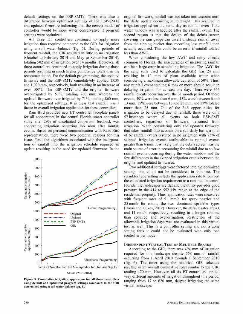
All three ET controllers continued to apply more irrigation than required compared to the GIR for irrigation using a soil water balance (fig. 5). During periods of frequent rainfall, the GIR resulted in little to no irrigation (October to February 2014 and May to September 2014), totaling 502 mm of irrigation over 14 months. However, all three controllers continued to apply irrigation during those periods resulting in much higher cumulative totals than the recommendation. For the default programming, the updated firmware and the ESP-SMTe cumulatively applied 1,039 and 1,020 mm, respectively, both resulting in an increase of over 100%. The ESP-SMTe and the original firmware over-irrigated by 51%, totaling 760 mm, whereas the updated firmware over-irrigated by 71%, totaling 860 mm, for the optimized settings. It is clear that rainfall was a factor in overall irrigation application for these controllers.
Rain Bird provided new ET controller faceplate panels for all cooperators in the central Florida smart controller study after 29% of unsolicited cooperator feedback was concerning irrigation occurring too soon after rainfall events. Based on personal communication with Rain Bird representatives, there were two potential reasons for this issue. First, the algorithms associated with the incorpora-tion of rainfall into the irrigation schedule required an update resulting in the need for updated firmware. In the
original firmware, rainfall was not taken into account until the daily update occurring at midnight. This resulted in irrigation applied on the same day as rainfall even if the water window was scheduled after the rainfall event. The second reason is that the design of the debris screen covering the rain gauge can divert unsteady rainfall away from the tipping bucket thus recording less rainfall than actually occurred. This could be an error if rainfall totaled less than AWC.
When considering the low AWC and rainy climate common to Florida, the inaccuracies of measuring rainfall can be a large error in scheduling irrigation. The AWC for the sand soils used to calculate the GIR was 24 mm resulting in 12 mm of plant available water when considering a maximum allowable depletion of 50%. Thus, any rainfall event totaling 6 mm or more should result in delaying irrigation for at least one day. There were 346 rainfall events occurring over the 31 month period. Of these events, 49% were less than 6 mm, 13% were between 6 and 13 mm, 15% were between 13 and 25 mm, and 23% totaled more than 25 mm. Out of the 346 opportunities for irrigation to be delayed due to rainfall, there were only 57 instances where all events on both ESP-SMT controllers, regardless of firmware, refrained from irrigation. When considering only the updated firmware that takes rainfall into account on a sub-daily basis, a total of 62 rainfall events resulted in no irrigation with 73% of skipped irrigation events attributable to rainfall events greater than 6 mm. It is likely that the debris screen was the main source of error in accounting for rainfall due to so few rainfall events occurring during the water window and the few differences in the skipped irrigation events between the original and updated firmwares.
Two additional settings were factored into the optimized settings that could not be considered in this test. The sprinkler type setting selects the application rate to convert the calculated irrigation requirement to a runtime. In central Florida, the landscapes are flat and the utility provides good pressure in the 414 to 552 kPa range at the edge of the residential property. Thus, application rates were measured with frequent rates of 51 mm/h for spray nozzles and 25 mm/h for rotors, the two dominant sprinkler types (Davis and Dukes, 2012). However, the default rates are 41 and 11 mm/h, respectively, resulting in a longer runtime than required and over-irrigation. Restriction of the allowable irrigation days was not evaluated in this virtual test as well. This is a controller setting and not a zone setting thus it could not be evaluated with only one controller per model.
INDEPENDENT VIRTUAL TEST OF MULTIPLE BRANDS According to the GIR, there was 494 mm of irrigation
required for this landscape despite 558 mm of rainfall occurring from 1 April 2010 through 1 September 2010 (fig. 6). The timer using the historical GIR schedule resulted in an overall cumulative total similar to the GIR, totaling 470 mm. However, all six ET controllers applied very different amounts of irrigation throughout this period, ranging from 17 to 620 mm, despite irrigating the same virtual landscape.
Figure 5. Cumulative irrigation application for all three controllersusing default and optimized program settings compared to the GIRdetermined using a soil water balance (eq. 1).
Cum
ulat
ive
Irri
gati
on
App
lica
tion
(m
m)
0
200
400
600
800
1000
1200
Month (2013-2014)
Sep Oct Nov Dec Jan Feb Mar Apr May Jun Jul Aug Sep Oct
Cum
ulat
ive
Irri
gati
on
App
lica
tion
(m
m)
0
200
400
600
800
1000
1200Original Updated ESP-SMTe GIR
Default Programming
Educational Programming
32(2): 251-262 261
The optimized settings of the R controller resulted in increased irrigation application compared to the R controller with restricted settings, which included water windows occurring two days per week and the use of landscape descriptions for program settings. The program setting optimization in this independent virtual test corresponded to the results for the ESP-SMT controllers with the original firmware, but contradicted the results of the ESP-SMT controllers with the updated firmware (table 6). Additionally, the other four ET controllers of varying brands had highly variable irrigation schedules despite irrigating the same virtual landscape. Thus, it is important to have knowledge concerning the algorithms and values associated with the settings as well as the way the controller uses those values based on both the brand and model of ET controller to irrigate efficiently. The effect of the program settings on the irrigation schedule would be beneficial to the professional installer in effort to maximize the water conservation potential of the technology.
CONCLUSION The newest Rain Bird ET controller, the ESP-SMTe,
consistently applied similar amounts of irrigation as the ESP-SMT with updated firmware, indicating that controller updates were minor between the two models. Plant types specific to central Florida were not a factor in irrigation application. However, selecting a heavier soil type, increasing the shade, and selecting a medium stand when a custom plant type was chosen resulted in reductions in irrigation application. These two controllers were different from the ESP-SMT with original firmware since the newer models applied more irrigation with identical programming.
The optimized settings on both newer models, selected as a combination of custom plant type, heavier soil type, increased shade, and medium stand, resulted in a reduction in irrigation application compared to the default values. Combining these custom settings with accurate sprinkler application rates and restricted irrigation days could produce an even larger reduction. As a result, these custom setting selections continue to be the UF-IFAS recommend-ed optimized settings for the Rain Bird ET controllers. However, an independent virtual test showed that selecting settings using a single landscape description (e.g., irrigation of St. Augustinegrass with spray heads on sand) resulted in highly variable irrigation totals, ranging from 17 to 620 mm, when evaluating multiple brands of ET controllers over an irrigation season. Thus, recommended settings cannot be generalized, making them specific to the ET controller brand and model. Despite the commitment of considerable time and effort, it is recommended that the user of the ET controller become familiar with the brand and model by observing the irrigation schedules after installation and adjusting the program settings to meet the needs of the landscape. Until manufacturers accept the benefits of increased technological adoption by end users from providing the algorithms behind the program settings, it would be advantageous to consult an irrigation professional or knowledgeable extension personnel to help with this process.
The accurate measurement and incorporation of rainfall into irrigation scheduling in Florida’s humid climate is extremely important due to frequent and variable rainfall events. However, these controllers were unable to fully account for rainfall throughout the virtual test. This can easily cause over-irrigation of 51-100%+ above the GIR. Increasing the accuracy of rainfall accounting would be extremely beneficial to overall water conservation and efficiency. Adjusting options for settings to allow for tailored irrigation schedules, such as being able to automatically adjust crop coefficients when increasing the root depth would also contribute to improved efficiency.
ACKNOWLEDGEMENTS The authors would like to thank the Water Research
Foundation, Orange County Utilities, St. John’s River Water Management District, South Florida Water Management District, and Florida Agricultural Experiment Station for their generous support of this research. We would also like to acknowledge Michael Gutierrez, Alessandra Smolek, Sara Wynn, Maria Zamora-Re, and Eliza Breder for their hard work and dedication to maintaining the quality of the research throughout their involvement in this study.
REFERENCES Allen, R. G. (2000). Using the FAO-56 dual crop coefficient
method over an irrigated region as part of an evapotranspiration intercomparison study. J. Hydrol., 229(2000), 27-41. http://dx.doi.org/10.1016/S0022-1694(99)00194-8
Figure 6. Cumulative irrigation was compared among five brands ofET controllers (labeled R, W, X, Y, and Z), an irrigation timer with arain sensor, and the GIR determined using a soil water balance (eq. 1)for a landscape description of bermudagrass on a sand in full sun.
Date (2010)
4/1 5/1 6/1 7/1 8/1 9/1
Cum
ulat
ive
Irri
gati
on A
ppli
cati
on (
mm
)
0
100
200
300
400
500
600
700
Dai
ly R
ainf
all (
mm
)
0
20
40
60
80
100
R (Restricted) R (Optimized) Timer W X Y Z GIR Rainfall
Allen, R. G., Pereira, L. S., Raes, D., & Smith, M. (1998). Crop evapotranspiration: Guidelines for computing crop requirements. Irrig. Drain. Paper No. 56. Rome, Italy: FAO.
ASCE Task Committee on Standardization of Reference Evapotranspiration. (2005). The ASCE standardized reference evapotranspiration equation. (R. G. Allen, Ed.) Reston, Va.: ASCE.
Cardenas-Lailhacar, B., & Dukes, M. D. (2012). Soil moisture sensor landscape irrigation controllers: A review of multi-study results and future implications. Trans. ASABE, 55(2), 581-590. http://dx.doi.org/10.13031/2013.41392
Ciach, G. J. (2003). Local random errors in tipping-bucket rain gauge measurements. J. Atmos. Oceanic Technol., 20, 752-759. http://dx.doi.org/10.1175/1520-0426(2003)20<752:LREITB>2.0.CO;2
Davis, S. L., & Dukes, M. D. (2010). Irrigation scheduling performance by evapotranspiration-based controllers. Agric. Water Manag., 98(2010), 19-28. http://dx.doi.org/10.1016/j.agwat.2010.07.006
Davis, S. L., & Dukes, M. D. (2012). Implementation of smart controllers in Orange County, Fla: Results from year 1. Irrig. Assoc. 2012 Int. Irrig. Show. Falls Church, Va.: Irrig. Assoc.
Davis, S. L., & Dukes, M. D. (2015a). Methodologies for successful implementation of smart irrigation controllers. J. Irrig. Drain. Eng., 141(3), 04014055. http://dx.doi.org/10.1061/(ASCE)IR.1943-4774.0000804
Davis, S. L., & Dukes, M. D. (2015b). Implementing smart controllers on single-family homes with excessive irrigation. J. Irrig. Drain. Eng., 141(12), 04015024. http://dx.doi.org/10.1061/(ASCE)IR.1943-4774.0000920
Davis, S. L., Dukes, M. D., & Miller, G. L. (2009). Landscape irrigation by evapotranspiration-based irrigation controllers under dry conditions in southwest Florida. Agric. Water Manag., 96(2009), 1828-1836. http://dx.doi.org/10.1016/j.agwat.2009.08.005
Devitt, D. A., Carstensen, K., & Morris, R. L. (2008). Residential water savings associated with satellite-based ET irrigation controllers. J. Irrig. Drain. Eng., 134(1), 74-82. http://dx.doi.org/10.1061/(ASCE)0733-9437(2008)134:1(74)
Dukes, M. D. (2012). Water conservation potential of landscape irrigation smart controllers. Trans. ASABE, 55(2), 563-569. http://dx.doi.org/10.13031/2013.41391
Gibeault, V. A., Cocker-ham, S., Henry, J. M., & Meyer, J. (1989). California turfgrass: Its use, water requirement and irrigation. Cal. Turfgrass Culture, 39(3), 1-9.
Habib, E., Krajewski, W., & Kruger, A. (2001). Sampling errors of tipping-bucket rain gauge measurements. J. Hydrol. Eng., 6(2), 159-166. http://dx.doi.org/10.1061/(ASCE)1084-0699(2001)6:2(159)
Haley, M. B., Dukes, M. D., & Miller, G. L. (2007). Residential irrigation water use in central Florida. J. Irrig. Drain. Eng., 133(5), 427-434. http://dx.doi.org/10.1061/(ASCE)0733-9437(2007)133:5(427)
Irrigation Association. (2005). Landscape irrigation scheduling and water management. Falls Church, Va: Irrig. Assoc.
Irrigation Association. (2008). Smart Water Application Technology (SWAT) turf and landscape irrigation equipment testing protocol for climatologically based controllers: 8th draft. Falls Church, Va.: Irrig. Assoc. Retrieved from www.irrigation.org
Jia, X., Dukes, M. D., & Jacobs, J. M. (2009). Bahiagrass crop coefficients from eddy correlation measurements in central Florida. J. Irrig. Sci., 28(1), 5-15. http://dx.doi.org/10.1007/s00271-009-0176-x
McCready, M. S., & Dukes, M. D. (2010). Landscape irrigation scheduling efficiency and adequacy by various control technologies. Agric. Water Manag., 98(4), 697-704. http://dx.doi.org/10.1016/j.agwat.2010.11.007
McCready, M. S., Dukes, M. D., & Miller, G. L. (2009). Water conservation potential of smart irrigation controllers on St. Augustinegrass. Agric. Water Manag., 96(2009), 1623-1632. http://dx.doi.org/10.1016/j.agwat.2009.06.007
Romero, C. C., & Dukes, M. D. (2014). Estimation and analysis of irrigation in single-family homes in central Florida. J. Irrig. Drain. Eng., 140(2), 04013011. http://dx.doi.org/10.1061/(ASCE)IR.1943-4774.0000656
U.S. Census Bureau. (2014). Florida passes New York to become the nation’s third most populous state, Census Bureau reports. Press Release CB14-232. Retrieved from http://www.census.gov/newsroom/press-releases/2014/cb14-232.html