Important ECG diagnosis aiding indices of ventricular

septal defect children with or without congestive

heart failure

Meihui Guo and Mong-Na Lo Huang

Dept. of Applied Mathematics, National Sun Yat-sen University, Kaohsiung, Taiwan

Tel: (886)-7-5252000 X-3820, X-3811

E-mail: guomh@math.nsysu.edu.tw, lomn@math.nsysu.edu.tw

Zhidong Bai

Dept. of Mathematics, National Univ. of Singapore, Singapore

Tel: (65)-874-2738

E-mail: matbaizd@leonis.nus.edu.sg

Kai-Sheng Hsieh

Pediatrics, Kaohsiung Veteran General Hospital, Kaohsiung, Taiwan

Important ECG diagnosis aiding indices of ventricular

defect children with or without congestive heart

failure

SUMMARY

In this paper, we perform a statistical study of the conventional RR intervals and two

newly defined PR′and RT intervals of ECG data. A quadratic classification rule is ap-

plied to extract several important ECG diagnosis-aiding indices among normal children

and children with ventricular septal defect (VSD) with or without congestive heart failure

(CHF). The results show that certain statistics computed from PR′, RR and RT intervals

are important diagnosis-aiding indices. Best classification vectors are searched for pairwise

classification. Two methods, minimum distance criterion and a two stage classification pro-

cedure, are considered for three way classification. Furthermore, logistic regression models

based on transformations of these important diagnosis-aiding indices are proposed. The

receiver operating characteristic curves of the proposed models show better performance

than those of linear and quadratic logistic models. In order to proceed this study, a com-

puter algorithm of automatically detecting the three intervals is developed and the related

ECG data are collected and analyzed. The algorithm is also enhanced with an outlier

detection procedure for the automatic measurements of the PR′and RT intervals.

1 Introduction

The incidence of congenital heart disease (CHD) is about 1% of the live births. This in-

cidence is about the same throughout the world. Of all the CHD, the ventricular septal

defect (VSD) commonly known as “ a hole in the heart” is the most common malformation

accounting for about 30% of the CHD. With the VSD, there is a communication between

the right and left ventricles and causes increased volumes, pressures on the right and left

ventricles and thus increased work-load for both right and left ventricles. Depending on

the size of the defect and the pressure in the pulmonary circulation, the defect may result

in variable degree of increased load to the heart and cause different degree of circulatory

disturbances. These circulatory disturbances, when prominent, are collectively called as

congestive heart failure (CHF). The symptoms of CHF includes increasing heart rate, in-

creasing respiratory rate, difficulty in breathing, swelling of legs, enlarged liver · · · and

so on. Thus, CHF represents a more severe form of symptoms in patients with VSD.

Many of the cases with VSD have benign natural course with possibility of spontaneous

closure or can be managed surgically with good result. But a number of them will develop

complications such as CHF, recurrent respiratory tract infection or irreversible pulmonary

hypertension. All of these complications are related to large amount of left to right shunt

and the resulting CHF. Therefore, early and correct recognition of VSD/CHF is very im-

portant for these patients. Generally speaking, the detection of VSD/CHF is based on

clinical evidence such as physical examination, history taking and many imaging modal-

ities. These conventional methods do have some limitations. Among them, subjectivity

and/or complexity are the most obvious ones. Therefore other adjunct methods should

be sought. In this study, we attempt to study the possible changes of electrocardiograph

(ECG) in patients with VSD/CHF using time-domain parameters. Our long term objective

is to establish an automatic diagnostic aiding system of some specific cardiovascular situ-

ations by the collected long term ECG data. At present, our goal is to identify important

1

classification variables of ECG which are useful in determining VSD/CHF status.

In the literature, the variables such as RR interval, PR interval, QT interval, P wave

and T wave are all well known to be significant characteristics of ECG. However, only RR

intervals have been studied systematically in the literature in terms of long term time series

spectral analysis, see for example Kluge et al.(1988), Yamamoto and Hughson(1991) and

Chan et al.(1996). In this paper, we will study not only the RR intervals but also two newly

defined intervals called PR′intervals (the intervals between the peaks of P waves and the

peaks of the consecutive QRS complex) and the RT intervals (the intervals between the

peaks of QRS complex and the consecutive peaks of T waves), see Fig. 1. These three

intervals represent different time intervals of the cardiac impulse transmission. The RR

interval records the time intervals from the peak of a ventricular depolarization to its next

peak. The electric activation process spreads through the sinus node and the A-V node then

to the whole cardiac muscle. The reciprocal of the RR interval is the instantaneous heart

rate. The PR′interval records the time interval from the peak of an atrial depolarization

to the next peak of the ventricular depolarization. The activation process only spreads

through the atrio-A-V nodal junction and part of the whole cardiac muscle. While the RT

interval is the time interval from the peak of a ventricular depolarization to the consecutive

peak of the ventricular polarization. The activation process does not spread through any

nodes. This interval also includes part of the recovery process. Our studies show that the

medians and the log transformed standard deviations of PR′, RR and RT intervals provide

additional information to differentiate normal children from VSD children with or without

CHF.

Note that this newly defined PR′interval is different from the PR interval defined in

medical science, which is the intervals starting from the onset of P wave and ending at

the onset of QRS complex (see Fig. 1). There are two reasons for us to analyze the PR′

interval instead of the conventional PR interval. The first reason is due to the difficulty of

2

identifying the onsets of P wave and QRS complex displayed on the monitor by computers.

In order to extract the feature characteristics of the conventional PR interval, generally a

bandpass filter (Tompkins, 1993) or wavelet transform (Li, Zheng and Tai, 1995) have to

be applied to the data first, then the intervals are computed based on the smoothed data.

Our proposed PR′intervals are extracted from the original data and are relatively easier

to be calculated. Secondly, in our preliminary study (Guo et al., 1997), we found that the

proposed PR′

interval and the conventional PR interval have strong correlation. Thus,

the results of PR′interval might be applied to the conventional PR interval. Based on the

similar reasons, we will analyze the RT interval instead of the conventional QT interval.

In order to analyze the ECG data more effectively, we develop a computer algorithm in

next section to calculate the PR′, RR and RT intervals. The algorithm is also enhanced

with an outlier detection procedure. Our objective is to correctly classify patients into

three groups: Normal, VSD without CHF and VSD with CHF. A quadratic classification

rule based on the medians and log transformed standard deviations of the PR′, RR and

RT intervals is applied to allocate the status of patients. By computing the specificities,

sensitivities and the odds ratios of the allocations, we select three sets of important ECG

diagnosis-aiding indices for various cardiovascular situation. Based on these indices, a two

stage classification procedure is introduced to classify patients of Normal, VSD without

CHF and VSD with CHF groups. Finally, logistic regression models were built based on

these diagnosis-aiding indices.

The article is organized as follows. In section 2, we describe the congenital heart

data set and the data collection procedure. In section 3, a quadratic classification rule is

introduced. The minimum distance criterion and a two stage classification procedure are

considered for three way classification. The logistic regression models are also introduced.

In section 4, the results of our empirical study are presented. Several important diagnosis-

aiding indices were extracted from the PR′, RR and RT intervals based on the classification

3

results. Logistic regression models and the Receiver Operating Characteristic (ROC) curves

are also generated. Discussion is given in section 5.

2 Congenital heart data set

This study is a joint project with Department of Pediatrics, Kaohsiung Veteran General

Hospital of Taiwan which is a major general hospital in southern Taiwan. We collect

data from patients in the cardio-vascular surgery intensive care unit three times a week.

The medical history of the patients are given. By connecting personal computer with

the HPM/1165A/66A Component Monitoring System, digitized ECG data is collected

and saved in a portable hard disk then brought back to the University to proceed further

analysis. Since the status of the patients are known beforehand, we perform a retrospective

study to classify patients into three groups (Normal, VSD with CHF and VSD without

CHF) by their ECG characteristics. In the following, we describe the three main steps in

collecting the data.

(A) First, the electrodes are stuck by nurses on patients’ chests, the electric waves pro-

duced by the cardiac physiological activities will then be transmitted by the elec-

trodes and forwarded to HPM/1165A/66A Component Monitoring System. At the

same time, the ECG waves will be shown on the monitor of the system.

(B) The analog signal converter (M1002A ECG/RESP) installed in the Monitoring System

will convert the ECG waves to analog signals and transmit to computer.

(C) The analog digital converter (Model PCL-818H High Performance Data Acquisition

Card) installed in the computer will then transfer the input analog signals to digital

signals. Finally, the digital signals are transferred to numerical read-out by the

computer software and stored in the hard disk of the computer.

4

In Fig. 2, we plot an example of the discrete ECG waves transferred by the computer. The

sampling rate of the computer is 1/500 second and the sampling duration is ten minutes.

There are approximate three hundred thousands points in a data set. In general, we collect

three consecutive ten-minute ECG data sets of each sampled patient. If interruptions occur,

fewer data sets might be collected. To avoid personal multiple effect, only one ten-minute

data set of each person is used in the analysis. Since the collected data is a long term

continuous ECG data, it is frequently interrupted by different kinds of intervention such as

patient’s irritation and routine medical treatment · · · etc. These unexpected interruptions

usually would cause abruptly variation of the collected ECG data, which makes the calcu-

lation of the interested intervals difficult or even impossible. To obtain computable data,

ECG data of the patients have to be collected again when the patients get back to stable

condition (e.g. no irritation or finish medical treatment). However due to the hospital

schedule, our data collection procedure is limited to two hours each day. In general, there

is no time left to collect the data again while interruptions occur. Therefore, collecting

usable data has been a difficult and time consuming task in our current research. Recently,

the hospital is planning to have an automatic ECG data collection system developed by a

computer company. After the system is implemented, we can collect long term data of all

patients monitored under the system remotely through the network between the hospital

and our university any time. By that time, computable data can be collected more easily.

In the past three years, we collected hundreds of data, among them there are 89 children

that can be classified into the three groups (Normal, VSD without CHF and VSD with

CHF). In this work, we study the ECG data sets of lead II of these 89 children ranged

from one month old to nine years old. In consideration of cardiac condition, data collected

from children under one month old is excluded from this study. Table 1 lists the clinical

profile of these children.

5

Table 1. List of data

Status Normal VSD without CHF VSD with CHFData No. 30 28 31

In general, there are approximate one thousand PR′, RR and RT intervals, respectively,

in a ten-minute ECG data. In order to calculate these intervals effectively, we develop the

following computer algorithm. For brevity, the peaks of QRS, T and P complexes will be

called Rmax, Tmax and Pmax, respectively.

Step-1 The first Rmax was searched using the following preset thresholds.

(i) For each ten minute data set, we define

index1 =1

5( max1≤i≤400

Vi − min1≤i≤400

Vi)

index2 =2

5( max1≤i≤400

Vi − min1≤i≤400

Vi),

where Vi denote the i-th recorded amplitude of the ECG data. We search the

first Vj such that

|Vj − Vj+3| > index1 and |Vj − Vj+6| > index2,

then search the maximum point of the nearby 25 points before and after Vj.

The first Rmax will be the maximum of {Vk, j − 25 ≤ k ≤ j + 25}.

(ii) The next Rmax is searched from the previous Rmax plus 50 points by repeating

(i). The searching process will keep on until all Rmax’s in the collection period

are found.

The number of points between the consecutive Rmax multiplied by 1/500 second is

the RR interval. We exam the plot of each ten minute RR intervals. If the plots

exhibit regular variation, then we proceed the following Step-2. If few outliers occur

in the plot, we will identify these points and correct the mistaken ones. If the plots

6

show large abnormal variation, then we will reset index1 and index2 to be the one

fifth and two fifth of the range of the first 600 recorded amplitudes, respectively. Then

apply these new indices to repeat (i). In our experience, this will fix the problem and

find the correct RR intervals.

Step-2 The first local maximum point behind the Rmax is Tmax. We search Tmax

between 20 points (= 0.04 second) after the Rmax and two-thirds of the total points

of the incident RR interval. For our data set, there are no Tmax’s occur outside the

range of 20 points and two-thirds RR interval. Yet for other ECG data of different

age groups, the searching range might have to be adjusted accordingly. The number

of points between Rmax and Tmax multiplied by 1/500 second is the RT interval.

Step-3 The first local maximum point behind the Tmax is Pmax. We search Pmax

between the points after Tmax and before the next Rmax minus 30 or 40 points. For

our data set, the time of 30 or 40 points (=0.08 second) is short enough to exclude

the occurrence of Pmax. The number of points between Pmax and the consecutive

Rmax multiplied by 1/500 second is the PR′interval.

Note that the quality of collected ECG is easily influenced by muscle related electric

noise, 60 Hz interference, baseline wander and T -wave interference, see for example Pan and

Tompkins (1985) and Hamilton and Tompkins (1986). These interferences may occasionally

induce incorrect automatic measurements of PR′and RT intervals, yet have little impact

on the measurements of the RR intervals. The error rates of the algorithm in searching the

RR intervals are below 5%. To exclude the noise artifact, we enhanced the above algorithm

with the following outlier detection procedure in searching PR′and RT intervals.

The sample autocorrelation functions (ACF) of PR′and RT intervals show slow decay,

yet the sample ACF of their corresponding first difference sequences, {∇PR} and {∇RT}

are analogous to that of moving average processes of orders 1 or 2 (see Fig. 5). Guo et

7

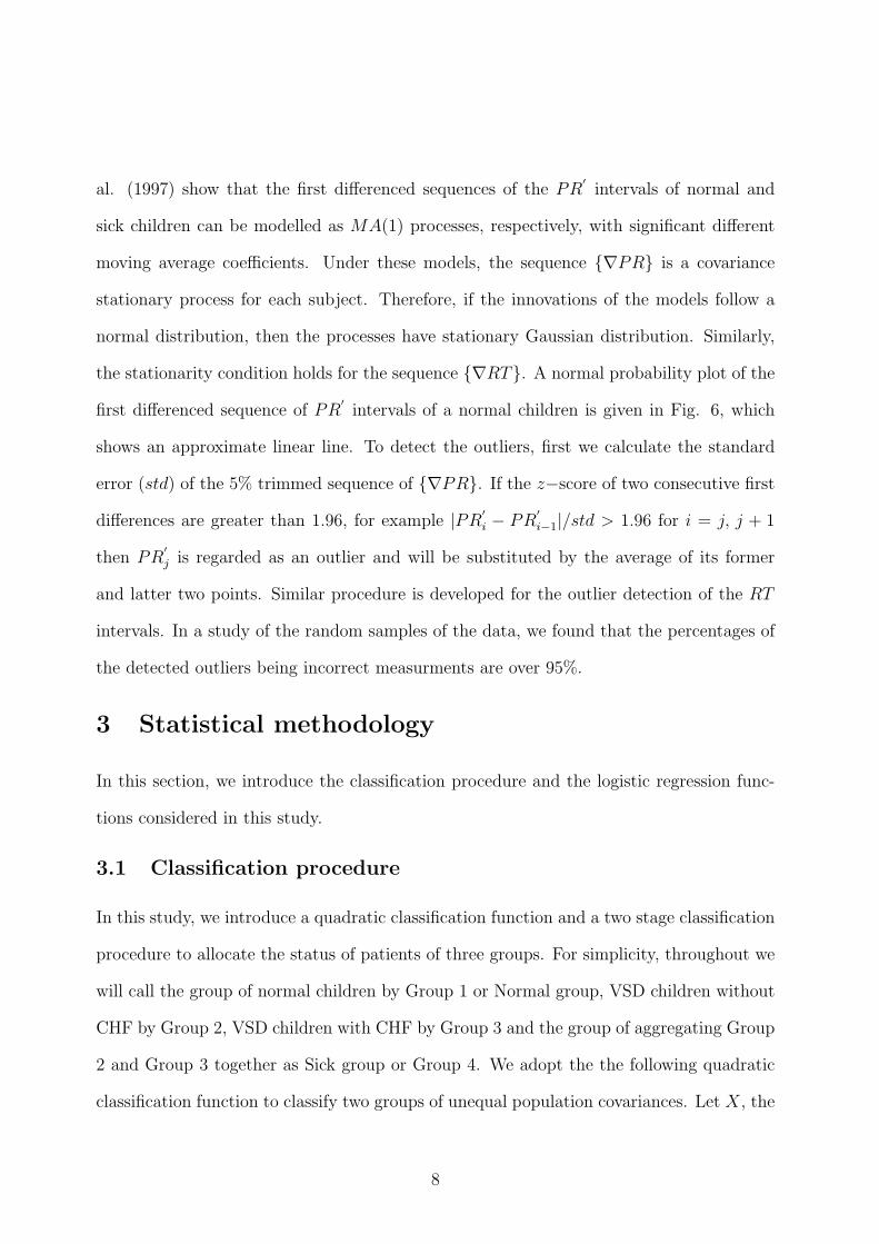
al. (1997) show that the first differenced sequences of the PR′

intervals of normal and

sick children can be modelled as MA(1) processes, respectively, with significant different

moving average coefficients. Under these models, the sequence {∇PR} is a covariance

stationary process for each subject. Therefore, if the innovations of the models follow a

normal distribution, then the processes have stationary Gaussian distribution. Similarly,

the stationarity condition holds for the sequence {∇RT}. A normal probability plot of the

first differenced sequence of PR′intervals of a normal children is given in Fig. 6, which

shows an approximate linear line. To detect the outliers, first we calculate the standard

error (std) of the 5% trimmed sequence of {∇PR}. If the z−score of two consecutive first

differences are greater than 1.96, for example |PR′i − PR

′i−1|/std > 1.96 for i = j, j + 1

then PR′j is regarded as an outlier and will be substituted by the average of its former

and latter two points. Similar procedure is developed for the outlier detection of the RT

intervals. In a study of the random samples of the data, we found that the percentages of

the detected outliers being incorrect measurments are over 95%.

3 Statistical methodology

In this section, we introduce the classification procedure and the logistic regression func-

tions considered in this study.

3.1 Classification procedure

In this study, we introduce a quadratic classification function and a two stage classification

procedure to allocate the status of patients of three groups. For simplicity, throughout we

will call the group of normal children by Group 1 or Normal group, VSD children without

CHF by Group 2, VSD children with CHF by Group 3 and the group of aggregating Group

2 and Group 3 together as Sick group or Group 4. We adopt the the following quadratic

classification function to classify two groups of unequal population covariances. Let X, the

8

classification vector, denote a subset vector of the following six interval statistics

X1 = (log s(PR′), m(PR

′), log s(RR), m(RR), log s(RT ), m(RT ))

′,

where m(·) and log s(·) and denote the medians and the logarithmic transformation of

the standard deviations of the intervals, respectively. Let the classification function be

Di(X) = (X − µi)′Σ−1

i (X − µi), where µi and Σi are the mean and covariance matrix of

the i-th group, i = 1, 2, 3, 4, respectively. The function Di(·) is also known as a Mahalanobis

distance (Mahalanobis, 1936, Rencher, 1995) which will be used to classify groups in Section

4.2. In practice, we use X̄i (the sample mean) and Si (the sample covariance matrix)

to estimate the unknown parameters µi and Σi, the resulting classification function are

denoted by D̂i(X). Let Dij(X) = D̂i(X) − D̂j(X), i = 1, j = 2, 3, 4 and i = 2, j = 3. For

Group i v.s. Group j, we assign a subject to Group i or Group j depending on its Dij(X)

is negative or positive. Throughout, we use a resubstitution method to classify a subject

and a retrospective study was performed based on the data listed in Table 1. The following

classification table, for example consider Group 1 v.s. Group 2, can then be obtained for

each classification vector X.

Table 2. Classification Table for Two GroupsActual group Predicted group observation no.

Group 1 Group 2Group 1 n11 n12 n1

Group 2 n21 n22 n2

The classification vector with the largest sensitivity (=n22/n2) and specificity (=n11/n1) is

considered as the best classification vector. In the case when the best classification vector

defined as above does not exist or is not unique, it is regarded as the one with the largest

odds ratio(= (n11n22)/(n12n21)) among those vectors with both sensitivity and specificity

greater than 0.7.

The best classification vectors of Group 1 v.s. Group 2, Group 1 v.s. Group 3, Group 2

v.s. Group 3 and Normal v.s. Sick will be searched in Section 4.2 for pairwise classification.

9

To further classify the three groups simultaneously, we consider two approaches. The first

method is to classify a subject to Group i if D̂i(X1) is the minimum of {D̂1(X1), D̂2(X1)

and D̂3(X1)}. The second approach is the following two stage classification procedure.

The classification results are given in Section 4.2.

(Stage-1) First, a subject is classified into Normal or Sick groups. The best classification vector

of Normal v.s. Sick is X1 (= the six interval statistics) with specificity = 0.733 and

sensitivity = 0.813. We found that the sensitivity can be further improved by using

the following rule. A subject is classified into Normal group if both its corresponding

D12(X1) and D13(X2) are less than 0, otherwise it is classified into Sick group. The

vectors X1 and X2 (see Section 4.2) are the best classification vectors of Group 1

v.s. Group 2 and Group 1 v.s. Group 3, respectively. Under this rule, a subject is

allocated to Normal group, if it is classified to Group 1 for both pair comparisons,

Group 1 v.s. Group 2 and Group 1 v.s. Group 3, based on their corresponding best

classification vectors.

(Stage-2) For subjects allocated into Sick group, they are further classified into Group 2 if their

D23(X3) < 0, or to Group 3 if their D23(X3) ≥ 0. The vector X3 denotes the best

classification vector of Group 2 v.s. Group 3.

3.2 Logistic Analysis

The logistic regression models are used to establish parametric relationship between the

classification vector X1 and the log-odds ln[P (Y =1|X1)P (Y =0|X1)

]. The notation Y = 1 represents

that a subject is allocated into the group of more sever symptom. For example, Y = 1

represents a subject is allocated to Group 2 for Group 1 v.s. Group 2; to Group 3 for

Group 1 v.s. Group 3 and Group 2 v.s. Group 3; to Sick group for Normal v.s. Sick

groups. Assume that P (Y = 0) = π0 and P (Y = 1) = π1 for some physically defined

probabilities π0 and π1. Denote the conditional probability of X1 given Y = j (j = 0, 1)

10

by fj(X1), then by Bayes’ theorem,

P (Y = 1|X1) =f1(X1)π1

f0(X1)π0 + f1(X1)π1

so that the log odds,

ln(P (Y = 1|X1)

P (Y = 0|X1)) = ln(

π1

π0

) + ln(f1(X1)

f0(X1)).

If the logistic p.d.f.

P (Y = 1|X1) =exp(α0 + α

′1X1)

1 + exp(α0 + α′1X1)

is adopted, the function ln(f1(X1)f0(X1)

) is a linear function of X1 and the following linear logistic

regression model can be build,

ln(P (Y = 1|X1)

P (Y = 0|X1)) = α0 + α

′

1X1 + ε. (1)

In next section, Model (1) will be built for Normal v.s. Sick and Group 2 v.s. Group 3,

respectively.

In this study, we propose to build the logistic regression models based on transforma-

tions of the best classification vectors. In Section 4.3, we will show the dominance of this

proposed model over the linear and quadratic models by the Receiver Operating Charac-

teristic (ROC) curves. In the following, we illustrate the idea of this new model. In many

cases, the function ln(f1(X1)f0(X1)

) can be expressed as a linear function of a transformation of

X1 (Kay and Little, 1987). For example, consider Group 1 v.s. Group 2, if f0(·) and f1(·)

both have the following elliptically symmetric distributions, f1(X) = |∑2 |−1/2q(D2(X))

and f0(X) = |∑1 |−1/2q(D1(X)), where D1 and D2 are defined as in Section 3.1 and q(·)

is a function on [0,∞), then

ln(f1(X1)

f0(X1)) = −1

2ln(

|∑2 ||∑1 |

) + ln(q(D2(X1))

q(D1(X1))).

In particular, if f0(·) and f1(·) are multivariate Normal distributions, then

ln(f1(X1)

f0(X1)) = −1

2ln(

|∑2 ||∑1 |

) +1

2(D1(X1)−D2(X1)).

11

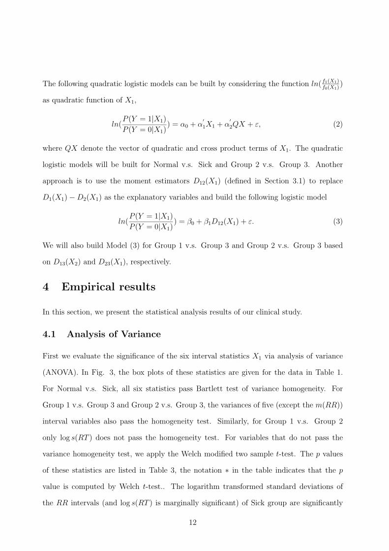
The following quadratic logistic models can be built by considering the function ln(f1(X1)f0(X1)

)

as quadratic function of X1,

ln(P (Y = 1|X1)

P (Y = 0|X1)) = α0 + α

′

1X1 + α′

2QX + ε, (2)

where QX denote the vector of quadratic and cross product terms of X1. The quadratic

logistic models will be built for Normal v.s. Sick and Group 2 v.s. Group 3. Another

approach is to use the moment estimators D12(X1) (defined in Section 3.1) to replace

D1(X1)−D2(X1) as the explanatory variables and build the following logistic model

ln(P (Y = 1|X1)

P (Y = 0|X1)) = β0 + β1D12(X1) + ε. (3)

We will also build Model (3) for Group 1 v.s. Group 3 and Group 2 v.s. Group 3 based

on D13(X2) and D23(X1), respectively.

4 Empirical results

In this section, we present the statistical analysis results of our clinical study.

4.1 Analysis of Variance

First we evaluate the significance of the six interval statistics X1 via analysis of variance

(ANOVA). In Fig. 3, the box plots of these statistics are given for the data in Table 1.

For Normal v.s. Sick, all six statistics pass Bartlett test of variance homogeneity. For

Group 1 v.s. Group 3 and Group 2 v.s. Group 3, the variances of five (except the m(RR))

interval variables also pass the homogeneity test. Similarly, for Group 1 v.s. Group 2

only log s(RT ) does not pass the homogeneity test. For variables that do not pass the

variance homogeneity test, we apply the Welch modified two sample t-test. The p values

of these statistics are listed in Table 3, the notation ∗ in the table indicates that the p

value is computed by Welch t-test.. The logarithm transformed standard deviations of

the RR intervals (and log s(RT ) is marginally significant) of Sick group are significantly

12

smaller than that of Normal group, which indicates the cardiac variability of Sick group

is less active. To evaluate the significance of the classification functions, we also perform

two sample t-test for D12(X1), D13(X2) and D23(X3). Their corresponding box plots are

given in Fig. 4. The result is listed in Table 4, all three variables are significant for each

pair comparison. We will show in Section 4.2, these statistics also play important roles

in classification and prediction. Also note that, for Group 1 v.s. Group 2, although none

of the interval statistics are significant, yet their function D12(X1) is significant in the

ANOVA.

Table 3. p values of the interval statisticslog s(PR

′) m(PR

′) log s(RR) m(RR) log s(RT ) m(RT )

Normal v.s. Sick 0.6182 0.2306 0.0483 0.1250 0.0614 0.1793Group1 v.s. Group2 0.7265 0.5926 0.7790 0.8239 0.2329∗ 0.7800Group1 v.s. Group3 0.2934 0.0131 0.0014 0.0033∗ 0.0638 0.0094Group2 v.s. Group3 0.1560 0.0012 0.0090 0.0017∗ 0.3622 0.0085

∗ indicates that the p values are computed by Welch t-test.

Table 4. p values of D12(X1), D13(X2) and D23(X3)D12(X1) D13(X2) D23(X3)

Normal v.s. Sick 0.0001 0.0003Group 1 v.s. Group 2 0.0003Group 1 v.s. Group 3 0.0001Group 2 v.s. Group 3 0.0001

4.2 Classification results

The selection of the best classification vectors is performed by a backward procedure. That

is we consider the six, five and four · · · interval statistics as the classification vectors step

by step. We compute the specificities, sensitivities and odds ratios of these classification

vectors then select the best ones according to the rule given in Section 3.1. The best

classification vector of Group 1 v.s. Group 2 is X1= the vector of six interval statistics; of

Group 1 v.s. Group 3 is X2 = (m(PR′), log s(PR

′), m(RR), m(RT ), log s(RT ))

′; of Group

2 v.s. Group 3 is X3 = (m(PR′), m(RR), m(RT ), log s(RT ))

′. In Table 5, we list the

13

sensitivities, specificities and odds ratios of X1, X2 and X3, respectively. Obviously, the

sensitivity of Group 2 v.s. Group 3 is the highest among the four cases.

Table 5. Specificities, sensitivities and odds ratios of X1, X2 and X3

Comparison pair Classification vector Specificity Sensitivity Odds ratioGroup 1 v.s. Group 2 X1 0.767 0.786 12.05Group 1 v.s. Group 3 X2 0.80 0.839 20.8

Normal v.s. Sick X1 0.733 0.813 12Normal v.s. Sick X1, X2(Stage− 1) 0.733 0.881 20.4

Group 2 v.s. Group 3 X3 0.75 0.903 28

For three way classification, we adopt two methods. In the first method, we allocate

subjects of three groups by the minimum of D̂1(X1), D̂2(X1), and D̂3(X1). In the second

method, we classify subjects by the two stage classification procedure introduced in Section

3.1. In Table 6, we list the correct classification rates of the three way classification by

these two methods. The results show that correct rates of the two stage classification are

slightly higher for both Group 2 and Group 3 .

Table 6. Correct classification rates of three way classification

classification method Group 1 Group 2 Group 3

min{D̂1, D̂2D̂3} 0.73 0.53 0.81Two stage method 0.73 0.57 0.87

To further investigate the two stage classification procedure, we show the dispersion situ-

ation of D12(X1) and D13(X2) of Normal v.s. Sick in Fig. 7. Since most of the subjects

in Normal group lie in the third quadrant and most subjects in Sick group lie in the other

three quadrants, the diagram justify the applicability of the classification rule of Stage-1.

Similarly for Group 2 v.s. Group 3, Fig. 8 shows the dispersion situation of D23(X3).

4.3 Logistic regression models

For linear and quadratic logistic models, we select the significant explanatory variables by

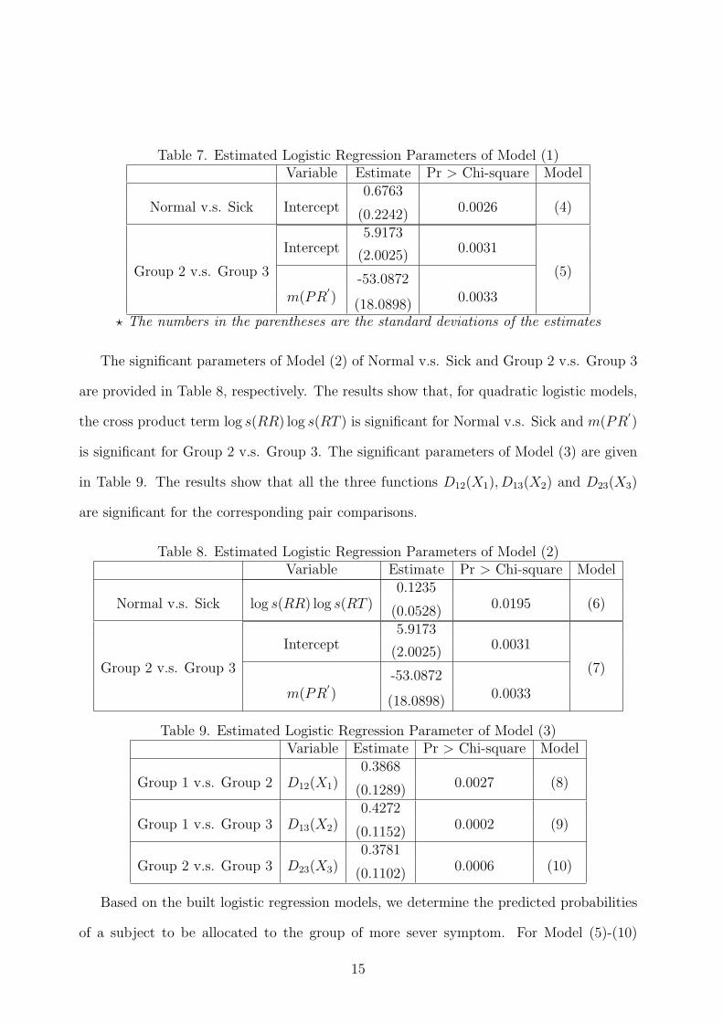
a forward stepwise procedure. The results of Table 7 show that for linear logistic model,

there is no significant explanatory variables for Normal v.s. Sick groups and m(PR′) is the

only significant variable for Group 2 v.s. Group 3.

14

Table 7. Estimated Logistic Regression Parameters of Model (1)Variable Estimate Pr > Chi-square Model

0.6763Normal v.s. Sick Intercept

(0.2242)0.0026 (4)

5.9173Intercept

(2.0025)0.0031

Group 2 v.s. Group 3-53.0872

(5)

m(PR′)

(18.0898)0.0033

? The numbers in the parentheses are the standard deviations of the estimates

The significant parameters of Model (2) of Normal v.s. Sick and Group 2 v.s. Group 3

are provided in Table 8, respectively. The results show that, for quadratic logistic models,

the cross product term log s(RR) log s(RT ) is significant for Normal v.s. Sick and m(PR′)

is significant for Group 2 v.s. Group 3. The significant parameters of Model (3) are given

in Table 9. The results show that all the three functions D12(X1), D13(X2) and D23(X3)

are significant for the corresponding pair comparisons.

Table 8. Estimated Logistic Regression Parameters of Model (2)Variable Estimate Pr > Chi-square Model

0.1235Normal v.s. Sick log s(RR) log s(RT )

(0.0528)0.0195 (6)

5.9173Intercept

(2.0025)0.0031

Group 2 v.s. Group 3-53.0872

(7)

m(PR′)

(18.0898)0.0033

Table 9. Estimated Logistic Regression Parameter of Model (3)Variable Estimate Pr > Chi-square Model

0.3868Group 1 v.s. Group 2 D12(X1) (0.1289)

0.0027 (8)

0.4272Group 1 v.s. Group 3 D13(X2) (0.1152)

0.0002 (9)

0.3781Group 2 v.s. Group 3 D23(X3) (0.1102)

0.0006 (10)

Based on the built logistic regression models, we determine the predicted probabilities

of a subject to be allocated to the group of more sever symptom. For Model (5)-(10)

15

(Model (4) is excluded, since only intercept is significant), we use the values C ∈ A =

{0.30, 0.35, · · · , 0.70, 0.75} as the ”cutpoints” for the probability of classifying individual

subjects to the group of more sever symptom. For each model, the sensitivity and specificity

are determined at each cutpoint and the Receiver Operating Characteristic (ROC) curves

can then be generated. For Normal v.s. Sick, we generate the ROC curves of Model (6)

and of considering Model (8) and Model (9) together. That is for a given cutpoint C, using

Stage-1 classification rule, if either of the predicted probabilities computed from Model (8)

or Model (9) is greater than C, then the subject is classified into Sick group. The results

of Normal v.s Sick and Group 2 v.s. Group 3 are given in Fig. 9 and Fig. 10, respectively.

The figures show that the specificities and sensitivities based on the predicted probabilities

of Model (3) dominate the linear and quadratic models. Furthermore, since Model (10)

do not include the intercept, the sensitivity and specificity at the cutpoint 0.5 ( e.g. when

D23(X3) = 0) are the same as that of the best classification vector for Group 2 v.s. Group

3. In such case, this approach will guarantee that one point of the R.O.C. curve has the

largest odds ratio than the other classification vectors.

5 Discussion

ECG is an economic and noninvasive tool of detecting cardiovascular situations. How-

ever, due to the lack of long term data and the difficulties of computing the conventional

quantities such as PR interval, P wave and T wave displayed on the monitor, a lot of the

information are not utilized or analyzed efficiently. In this research, we have proposed two

newly defined PR′and RT intervals to analyze the ECG data, which are relatively easier

to calculate and their corresponding statistics can efficiently differentiate among normal

children and VSD children with or without CHF. In the future, we plan to apply the results

to establish a diagnosis-aiding rule for normal children v.s. VSD/CHF children in clinical

trial. The long term goal is to implement an automatic diagnostic aiding system. Further-

16

more, the Mahalanobis distance has been used here successfully as a classification function.

By applying functions of the Mahalanobis distance, we built the logistic regression Model

(3). Compared with Model (1) and Model (2), the R.O.C. curve of Model (3) show better

performance for Normal v.s. Sick and Group 2 v.s. Group 3.

Acknowledgements

This research was supported in part by the grants NSC 87-2118-M-110-004 and NSC 87-

2118-M-075B-001 from the National Science Council of Taiwan.

REFERENCES

1. Chan, H.L., Lin, J.L., Du, C.C., Lin,I.N., Lin, K.T., Wu, C. P. and Lien, W.P. ‘The high-

resolution time-frequency characteristics of slower frequency heart rate variability in

patients of chronic refractory congestive heart failure- the implications of beta-blocker

therapy.’ Biomedical Engineering Applications, Basis & Communications 8, 447-461

(1996).

2. Guo, M., Huang, M.N. L., Bai, Z.D., Chen, H.T. and Hsieh K.S. ‘Statistical analysis

and modelling for PR Intervals of ECG.’ Journal of Chinese Statistical Association

35, 1-25 (1997).

3. Hamilton, P.S. and Tompkins W.J. ‘Quantitative investigation of QRS detection rules

using MIT/BIH arrhythmia database.’ IEEE Transactions on Biomedical Engineer-

ing BME-33, 1157-1187 (1986).

4. Kay, R. and Little S. ‘Transformations of the explanatory variables in the logistic re-

gression model for binary data.’ Biometrika 74, 495-501 (1987).

5. Kluge, K.A., Happer, R.M., Schechtman, V.L., Wilson, A.J., Hoffman, H.J., and

Southall, D.P. ‘Spectral analysis accessment of respiratory sinus arrhythmia in nor-

17

mal infants who subsequently died of sudden Infant Death Syndrome.’ Pediatric

Research 24, 677-682 (1988).

6. Li, C., Zheng, C. and Tai, C. ”Detection of ECG characteristic points using wavelet

transforms. IEEE Transactions on Biomedical Engineering BME 42, 2-28 (1995).

7. Mahalanobis, P.C. ‘On the generalized distance in statistics.’ Proceedings of the Na-

tional Institute of Sciences of India 12, 49-55 (1936).

8. Pahlm, O., Case D., Howard, G., Pope, J. and Kaisty, W.K. ‘Decision rules for the ECG

diagnosis of inferior myocardial infarction.’ Computers and Biomedical Research 23,

332-345 (1990).

9. Pan, J. and Tompkins, W.J. ‘A real-time QRS detection algorithm.’ IEEE Transactions

on Biomedical Engineering BME-32, 230-236 (1985).

10. Rencher, A.C. Methods of Multivariate Analysis. John Wiley & Sons, Inc., New York

(1995).

11. Tompkins, W.J. Biomedical digital signal processing : C-Language examples and lab-

oratory experiments for the IBM PC. Englewood Cliffs, N.J. : Prentice Hall (1993).

12. Yamamoto, Y. and Hughson, R.L. ‘Coarse-graining spectral analysis: new method for

studying heart rate variability.’ Journal of Applied Physiology 74, 1143-1150 (1991).

18

Fig. 1 ECG of Normal sinus Beat (Lead II)

19

Fig. 2 Discrete ECG Collected by Computer

20

Fig. 3 Box Plots of Interval Statistics

Fig. 4 Box plots of D12(X1), D13(X2) and D23(X3)

21

Fig. 6 Normal Probability Plot of ∇PR

22

Fig. 7 Dispersion of D12(X1) and D13(X2), Normal v.s. Sick

Fig. 8 Dispersion of D23(X3), Group2 v.s. Group3

23

24