JSS Journal of Statistical Software April 2009, Volume 30, Issue 4. http://www.jstatsoft.org/ Importing Vector Graphics: The grImport Package for R Paul Murrell The University of Auckland Abstract This article describes an approach to importing vector-based graphical images into statistical software as implemented in a package called grImport for the R statistical com- puting environment. This approach assumes that an original image can be transformed into a PostScript format (i.e., the opriginal image is in a standard vector graphics format such as PostScript, PDF, or SVG). The grImport package consists of three components: a function for converting PostScript files to an R-specific XML format; a function for read- ing the XML format into special Picture objects in R; and functions for manipulating and drawing Picture objects. Several examples and applications are presented, including annotating a statistical plot with an imported logo and using imported images as plotting symbols. Keywords : PostScript, R, statistical graphics, XML. 1. Introduction One of the important features of statistical software is the ability to create sophisticated statistical plots of data. Software systems such as the lattice (Sarkar 2008) package in R (R Development Core Team 2008) can produce complex images from a very compact expression. For example, the following code is all that is needed to produce the image in Figure 1, which shows density estimates for the number of moves in a set of chess games, broken down by the result of the games. R> xyplot(Freq ~ nmoves | result, data = chess.df, type = "h", + layout = c(1, 3), xlim = c(0, 100)) On the other hand, statistical graphics software does not typically provide support for pro- ducing more free-form or artistic graphical images. As a very simple example, it would be
This article describes an approach to importing vector-based graphical images intostatistical software as implemented in a package called grImport for the R statistical com-puting environment. This approach assumes that an original image can be transformedinto a PostScript format (i.e., the opriginal image is in a standard vector graphics formatsuch as PostScript, PDF, or SVG). The grImport package consists of three components: afunction for converting PostScript files to an R-specific XML format; a function for read-ing the XML format into special Picture objects in R; and functions for manipulatingand drawing Picture objects. Several examples and applications are presented, includingannotating a statistical plot with an imported logo and using imported images as plottingsymbols.
One of the important features of statistical software is the ability to create sophisticatedstatistical plots of data. Software systems such as the lattice (Sarkar 2008) package in R (RDevelopment Core Team 2008) can produce complex images from a very compact expression.For example, the following code is all that is needed to produce the image in Figure 1, whichshows density estimates for the number of moves in a set of chess games, broken down by theresult of the games.
R> xyplot(Freq ~ nmoves | result, data = chess.df, type = "h",
+ layout = c(1, 3), xlim = c(0, 100))
On the other hand, statistical graphics software does not typically provide support for pro-ducing more free-form or artistic graphical images. As a very simple example, it would be
2 Importing Vector Graphics: The grImport Package for R
nmoves
Fre
q
0
2
4
6
20 40 60 80
win0
2
4
6draw
0
2
4
6loss
Figure 1: A statistical plot produced in R using the lattice package. The data are from chessgames involving Louis Charles Mahe De La Bourdonnais between 1821 and 1838 (originalsource: http://www.chessgames.com/).
Figure 2: A free-form image of a chess pawn. This is an example of the sort of artistic graphicthat is difficult to produce using statistical software.
difficult to produce an image of a chess piece, like the pawn shown in Figure 2, using statisticalsoftware.
In the case of R, there is a general polygon-drawing function, but determining the verticesfor the boundary of this pawn image would be non-trivial. These sorts of artistic images areproduced much more easily using the tools that are provided by drawing software such asthe GIMP (Kylander and Kylander 1999, http://www.gimp.org/) or Inkscape (Bah 2007,http://www.inkscape.org/), not to mention that producing an aesthetically pleasing resultfor this sort of image also requires a healthy dose of artistic skill.
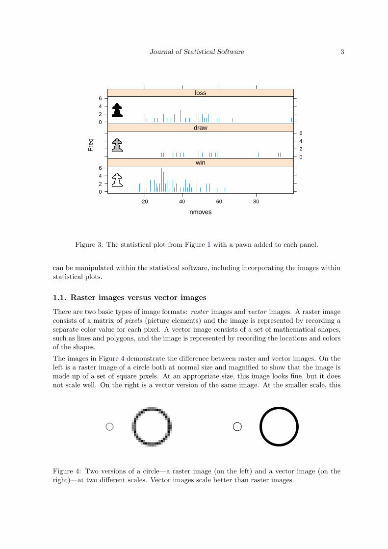
However, there are situations where it is useful to be able to include artistic images as partof a statistical plot. Figure 3 demonstrates this sort of annotation by adding a pawn to eachpanel of the plot from Figure 1, to provide an additional visual cue as to whether the gamesin the panel were won (white pawn), drawn (grey pawn) or lost (black pawn).
This is one example of the problem that is addressed in this article. Stating the issue moregenerally, this article is concerned with the ability to import graphical images that have beengenerated using third party software into a statistical software system so that the images
Figure 3: The statistical plot from Figure 1 with a pawn added to each panel.
can be manipulated within the statistical software, including incorporating the images withinstatistical plots.
1.1. Raster images versus vector images
There are two basic types of image formats: raster images and vector images. A raster imageconsists of a matrix of pixels (picture elements) and the image is represented by recording aseparate color value for each pixel. A vector image consists of a set of mathematical shapes,such as lines and polygons, and the image is represented by recording the locations and colorsof the shapes.
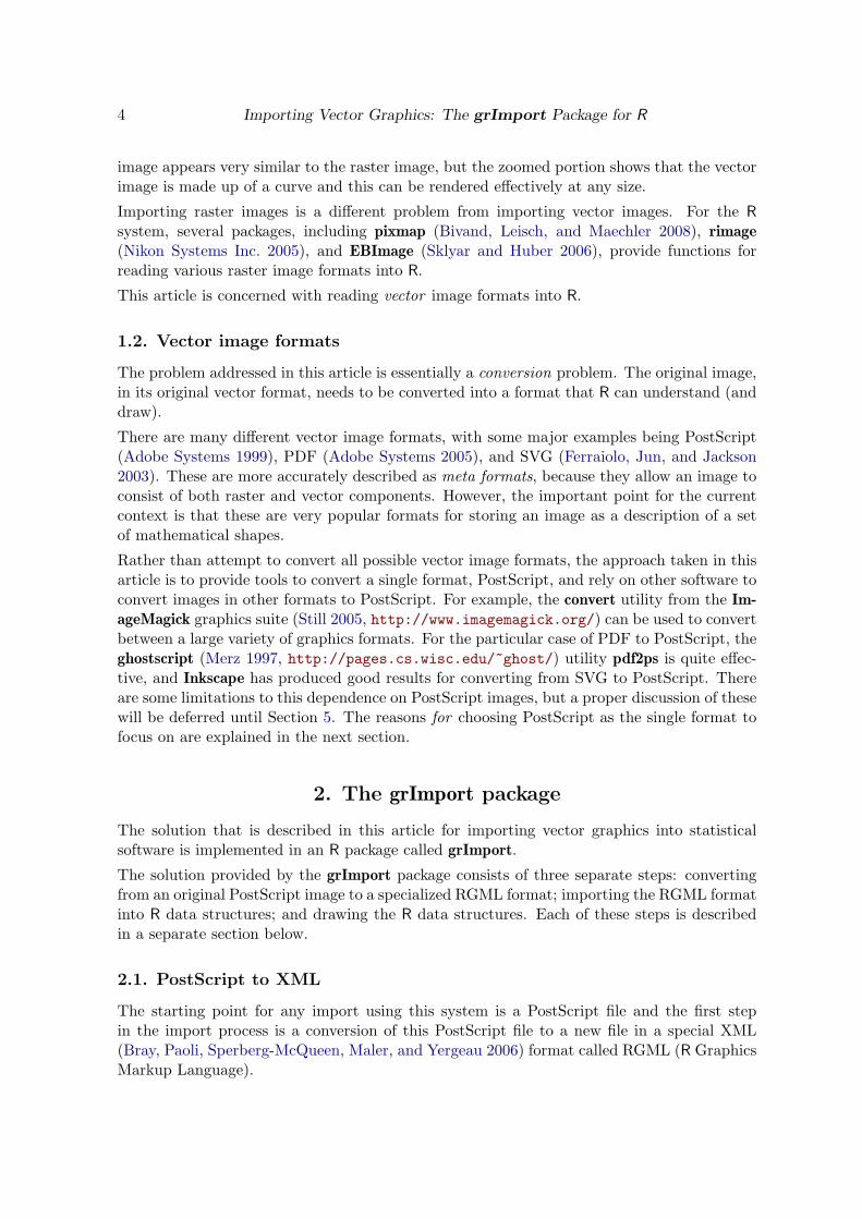
The images in Figure 4 demonstrate the difference between raster and vector images. On theleft is a raster image of a circle both at normal size and magnified to show that the image ismade up of a set of square pixels. At an appropriate size, this image looks fine, but it doesnot scale well. On the right is a vector version of the same image. At the smaller scale, this
●
Figure 4: Two versions of a circle—a raster image (on the left) and a vector image (on theright)—at two different scales. Vector images scale better than raster images.
4 Importing Vector Graphics: The grImport Package for R
image appears very similar to the raster image, but the zoomed portion shows that the vectorimage is made up of a curve and this can be rendered effectively at any size.
Importing raster images is a different problem from importing vector images. For the Rsystem, several packages, including pixmap (Bivand, Leisch, and Maechler 2008), rimage(Nikon Systems Inc. 2005), and EBImage (Sklyar and Huber 2006), provide functions forreading various raster image formats into R.
This article is concerned with reading vector image formats into R.
1.2. Vector image formats
The problem addressed in this article is essentially a conversion problem. The original image,in its original vector format, needs to be converted into a format that R can understand (anddraw).
There are many different vector image formats, with some major examples being PostScript(Adobe Systems 1999), PDF (Adobe Systems 2005), and SVG (Ferraiolo, Jun, and Jackson2003). These are more accurately described as meta formats, because they allow an image toconsist of both raster and vector components. However, the important point for the currentcontext is that these are very popular formats for storing an image as a description of a setof mathematical shapes.
Rather than attempt to convert all possible vector image formats, the approach taken in thisarticle is to provide tools to convert a single format, PostScript, and rely on other software toconvert images in other formats to PostScript. For example, the convert utility from the Im-ageMagick graphics suite (Still 2005, http://www.imagemagick.org/) can be used to convertbetween a large variety of graphics formats. For the particular case of PDF to PostScript, theghostscript (Merz 1997, http://pages.cs.wisc.edu/~ghost/) utility pdf2ps is quite effec-tive, and Inkscape has produced good results for converting from SVG to PostScript. Thereare some limitations to this dependence on PostScript images, but a proper discussion of thesewill be deferred until Section 5. The reasons for choosing PostScript as the single format tofocus on are explained in the next section.
2. The grImport package
The solution that is described in this article for importing vector graphics into statisticalsoftware is implemented in an R package called grImport.
The solution provided by the grImport package consists of three separate steps: convertingfrom an original PostScript image to a specialized RGML format; importing the RGML formatinto R data structures; and drawing the R data structures. Each of these steps is describedin a separate section below.
2.1. PostScript to XML
The starting point for any import using this system is a PostScript file and the first stepin the import process is a conversion of this PostScript file to a new file in a special XML(Bray, Paoli, Sperberg-McQueen, Maler, and Yergeau 2006) format called RGML (R GraphicsMarkup Language).
%!PSnewpath % start a new shape0 0 moveto % move to a start location-5 10 lineto % line to a new location-10 20 10 20 5 10 curveto % curve to a third location5 10 lineto % line to a fourth locationclosepath % connect back to the start location0 setgray % set the drawing colour to blackfill % fill the current shape
Table 1: The file petal.ps, which contains PostScript code to draw a simple “petal” shape(shown to the right of the code).
The RGML format is specific to the grImport package. It is a very simple graphics formatthat describes an image in terms that the R graphics system can understand. It will bedescribed in more detail in later sections.
As a simple example to follow through in detail, Table 1 shows a file, petal.ps, that consistsof PostScript code for drawing a simple “petal” shape, which is shown to the right of the codein Table 1.
This simple example demonstrates some basic PostScript commands. A shape, called a path,is defined by specifying lines and curves between a set of points and this shape is then filledwith a color.
Another common PostScript operation involves drawing just the boundary outline of theshape. This could be achieved in the example in Table 1 by replacing the command fill (thelast line of Table 1) with the command stroke (PostScript calls drawing the outline strokinga path).
The user interface provided by grImport for the conversion from PostScript to RGML formatis very simple, consisting of a single function, PostScriptTrace(). In the most basic usage,the only required argument is the name of the PostScript file to convert, as in the code below.The resulting RGML file, petal.ps.xml is shown in Table 2.
R> PostScriptTrace("petal.ps")
The RGML format in this example is roughly a one-to-one translation of the PostScript code.The shape is recorded as a <path> element that has a type attribute with the value fillindicating that the shape should be filled. The <context> element for this shape specifies thecolour to be used to fill the shape and then a series of <move> and <line> elements describethe outline of the shape itself. A <summary> element provides information on how many pathsthere are in the image, plus bounding box information.
One detail to notice is that the curveto in the PostScript file has become a series of <line>elements in the RGML file. We will discuss this issue further in Section 3. The main pointto focus on for now is that the image has become a set of (x, y) locations that describe theoutline of the shape in the image, as illustrated in Figure 5.
One reason for choosing PostScript as the original format to focus on is that it is a sophis-ticated graphics language. PostScript has commands to draw a wide variety of shapes and
6 Importing Vector Graphics: The grImport Package for R
Table 2: The file petal.ps.xml, which contains RGML code created by callingPostScriptTrace() on the PostScript code in Table 1.
Journal of Statistical Software 7
●
●
●
●●
● ● ● ●●●
●●
●
Figure 5: The PostScriptTrace() function breaks a path into a series of locations on theboundary of the path. This image shows how the curved petal shape from Table 1 can beconverted into a set of points describing the outline of the petal shape.
Table 3: The file flower.ps, which contains PostScript code to draw a simple “flower” shape(shown to the right of the code).
PostScript provides advanced facilities to control the placement of shapes and to controlsuch things as the colors and line styles for filling and stroking the shapes. This means thatPostScript is capable of describing very complex images; by focusing on PostScript we shouldbe able to import virtually any vector image no matter how complicated it is.
This is not to say that PostScript is the most sophisticated graphics language—PDF and SVGare also sophisticated graphics languages with various strengths and weaknesses compared toPostScript. The point is that, amongst graphics formats, PostScript is one of the sophisticatedones.
PostScript is also a complete programming language. As a simple demonstration of this,Table 3 shows a file, flower.ps, that contains PostScript code for drawing a simple “flower”shape, which is shown to the right of the code in Table 3.
The important feature of this PostScript code is that it defines a “macro” that describes howto draw a petal, then it runs this macro five times (at five different angles) to produce theoverall flower.
This complexity presents an imposing challenge for us. How can we convert PostScript codewhen the code can be extremely complicated? The approach taken by the grImport packageis to use the power of PostScript against itself.
8 Importing Vector Graphics: The grImport Package for R
%!PS/printtwo {
/printnum {100 mul round 100 div 20 string cvs print
Table 4: The file convert.ps, which contains PostScript code to process the PostScript filepetal.ps.
The first part of the solution is based on the fact that it is possible to write PostScript codethat runs other PostScript code. The basis for the conversion from an original PostScript fileto an RGML file is a set of additional PostScript code that processes the original PostScriptfile.
The other part of the solution is based on the fact that it is possible to redefine some ofthe core PostScript commands. For example, the grImport PostScript code redefines themeaning of the PostScript commands stroke and fill so that, instead of drawing shapes,these commands print out information about the shapes that would have been drawn.
Table 4 shows a very simplified version of how the grImport PostScript conversion codeworks. This code first defines a macro, printtwo that prints out two values. It also definesa macro, donothing, which does nothing. The next macro, fill, is the important one.This is redefining the standard PostScript fill command. This macro, instead of filling ashape, breaks any curves in the current path into short line segments (flattenpath), then itcalls the pathforall command. This command converts the current path into four possibleoperations: a move, a line, a curve, or a closing of the path (joining the last location in thepath back to the first location in the path). The four values in front of pathforall specifywhat to do for each of these operations. Overall, the code says that, if there is a move or aline in the path, then we should print out two values (the position moved to or the position“lined” to). For curves and closes, we do nothing. The final line of code in Table 4 says torun the PostScript code in the file petal.ps.
The PostScript code in the grImport package is a lot more complicated than the code inTable 4, but this demonstrates the main idea.
At this point, we have new PostScript code that can process the original PostScript code andprint out information about the shapes in the original image. However, we still need softwareto run the new PostScript code. The grImport package uses ghostscript for this purpose. For
Journal of Statistical Software 9
example, the code below shows how to run the simplified conversion code in Table 4, with theresulting output shown below that. Several of the values printed out should be recognisablefrom the PostScript code in the file petal.ps (see Table 1).
This dependence means that ghostscript must be installed for the grImport package to work,but it is readily available for all major platforms. On Windows, the R_GSCMD environmentvariable may also need to be set appropriately.
The beauty of this solution is that, no matter how complicated the PostScript code gets, itultimately calls stroke or fill to do the actual drawing. For example, the code in Table 3performs a loop to draw five petals, but we do not have to write code that understandsPostScript loops; all we have to do is to ensure that whenever the PostScript code ultimatelytries to fill one of the petals, we intervene and simply print out the information about thepetal instead.
Table 5 shows the RGML file that results from running PostScriptTrace() on the PostScriptcode in the file flower.ps. Many of the <line> elements have been left out in order to showthe overall structure of the file.
R> PostScriptTrace("flower.ps")
The overall effect is that the PostScript program in the file flower.ps has become a muchlonger, but much simpler RGML file consisting simply of descriptions of the five shapes thatwould have been drawn if the PostScript file had been viewed normally. The PostScript codethat is used to perform the conversion from the original PostScript file to an RGML file canbe found within the file PostScript2RGML.R of the grImport package.
At this point, there might appear to be little cause for celebration. All that we have managedto achieve is to convert the PostScript file into an RGML file. It is important to highlighthow much closer that has taken us to working with the image in R.
The main point is that the RGML format is simple. An RGML file only contains shapedescriptions, so all R has to do is read the information about each shape and draw it. Itis also important that the shape descriptions are simple enough for R to be able to draw(the R graphics system does not have some of the sophisticated features of the PostScriptformat). With the XML package (Temple Lang 2008), reading an XML file into R is relativelystraightforward and R has facilities for drawing each of the shapes in the RGML file.
10 Importing Vector Graphics: The grImport Package for R
Table 5: The file flower.ps.xml, which contains RGML code created by callingPostScriptTrace() on the PostScript code in Table 3. Most of the <line> elements havebeen removed and replaced with ... so that the overall structure of the complete file can bedisplayed.
Journal of Statistical Software 11
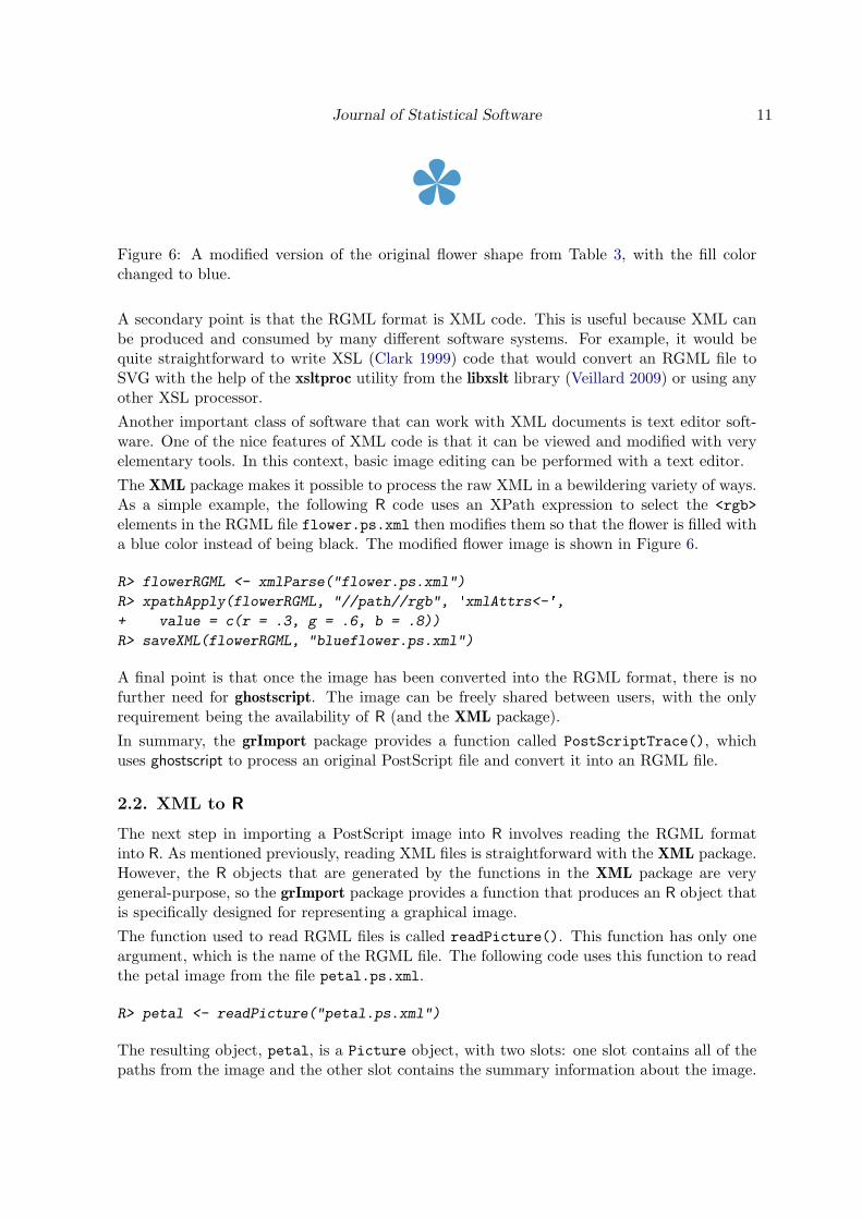
Figure 6: A modified version of the original flower shape from Table 3, with the fill colorchanged to blue.
A secondary point is that the RGML format is XML code. This is useful because XML canbe produced and consumed by many different software systems. For example, it would bequite straightforward to write XSL (Clark 1999) code that would convert an RGML file toSVG with the help of the xsltproc utility from the libxslt library (Veillard 2009) or using anyother XSL processor.Another important class of software that can work with XML documents is text editor soft-ware. One of the nice features of XML code is that it can be viewed and modified with veryelementary tools. In this context, basic image editing can be performed with a text editor.The XML package makes it possible to process the raw XML in a bewildering variety of ways.As a simple example, the following R code uses an XPath expression to select the <rgb>elements in the RGML file flower.ps.xml then modifies them so that the flower is filled witha blue color instead of being black. The modified flower image is shown in Figure 6.
A final point is that once the image has been converted into the RGML format, there is nofurther need for ghostscript. The image can be freely shared between users, with the onlyrequirement being the availability of R (and the XML package).In summary, the grImport package provides a function called PostScriptTrace(), whichuses ghostscript to process an original PostScript file and convert it into an RGML file.
2.2. XML to R
The next step in importing a PostScript image into R involves reading the RGML formatinto R. As mentioned previously, reading XML files is straightforward with the XML package.However, the R objects that are generated by the functions in the XML package are verygeneral-purpose, so the grImport package provides a function that produces an R object thatis specifically designed for representing a graphical image.The function used to read RGML files is called readPicture(). This function has only oneargument, which is the name of the RGML file. The following code uses this function to readthe petal image from the file petal.ps.xml.
R> petal <- readPicture("petal.ps.xml")
The resulting object, petal, is a Picture object, with two slots: one slot contains all of thepaths from the image and the other slot contains the summary information about the image.
12 Importing Vector Graphics: The grImport Package for R
In this case, there is only one path and it is a PictureFill object (i.e., a shape that shouldbe filled with a color).
R> str(petal)
Formal class 'Picture' [package "grImport"] with 2 slots..@ paths :List of 1.. ..$ path:Formal class 'PictureFill' [package "grImport"] with 4 slots.. .. .. ..@ x : Named num [1:36] 0 -50 -54 -56.6 -57.9 ..... .. .. .. ..- attr(*, "names")= chr [1:36] "move" "line" "line" "line" ..... .. .. ..@ y : Named num [1:36] 0 100 109 118 125 ..... .. .. .. ..- attr(*, "names")= chr [1:36] "move" "line" "line" "line" ..... .. .. ..@ rgb: chr "#000000".. .. .. ..@ lwd: num 1.33..@ summary:Formal class 'PictureSummary' [package "grImport"] with 3 slots.. .. ..@ numPaths: Named num 1.. .. .. ..- attr(*, "names")= chr "count".. .. ..@ xscale : Named num [1:2] -58 58.. .. .. ..- attr(*, "names")= chr [1:2] "xmin" "xmax".. .. ..@ yscale : Named num [1:2] 0 175.. .. .. ..- attr(*, "names")= chr [1:2] "ymin" "ymax"
The Picture object has a clear one-to-one correspondence with the information in the XMLfile and, again, we might question what we have gained by generating this object. Why notjust draw the information from the RGML file directly?The main reason for having the special S4 class of Picture objects in R is that we can workwith the image using all of the powerful data processing tools that are available in R. Onespecific example that is explicitly supported by the grImport package is the ability to subsetpaths from an image.As a simple example of subsetting, consider the Picture object that is generated by readingin the RGML file that was generated from the PostScript file flower.ps (see Table 5). Onlythe summary information for this Picture object is shown.
R> PSflower <- readPicture("flower.ps.xml")
R> str(PSflower@summary)
Formal class 'PictureSummary' [package "grImport"] with 3 slots..@ numPaths: Named num 5.. ..- attr(*, "names")= chr "count"..@ xscale : Named num [1:2] 29.6 370.4.. ..- attr(*, "names")= chr [1:2] "xmin" "xmax"..@ yscale : Named num [1:2] 44.1 375.. ..- attr(*, "names")= chr [1:2] "ymin" "ymax"
This Picture object has five paths, corresponding to the five petals. A subsetting methodfor Picture objects is defined by the grImport package so that we can extract just some ofthe petals from the image as shown in the code below.
Journal of Statistical Software 13
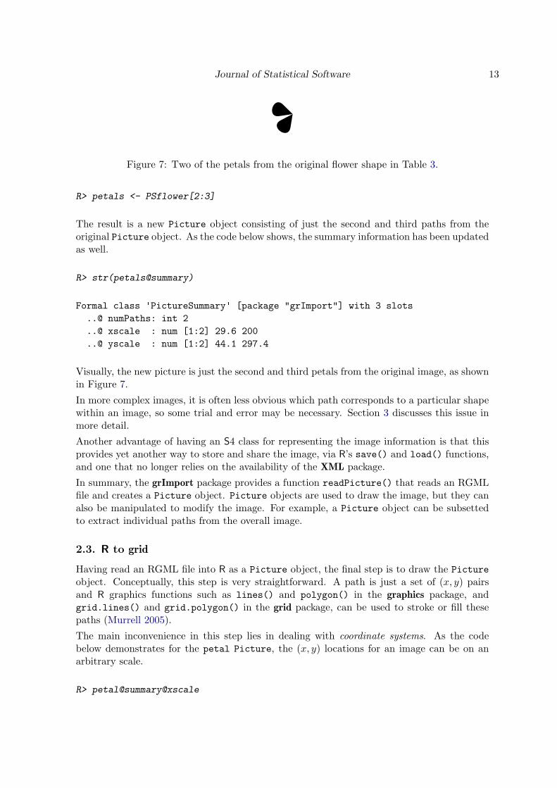
Figure 7: Two of the petals from the original flower shape in Table 3.
R> petals <- PSflower[2:3]
The result is a new Picture object consisting of just the second and third paths from theoriginal Picture object. As the code below shows, the summary information has been updatedas well.
R> str(petals@summary)
Formal class 'PictureSummary' [package "grImport"] with 3 slots..@ numPaths: int 2..@ xscale : num [1:2] 29.6 200..@ yscale : num [1:2] 44.1 297.4
Visually, the new picture is just the second and third petals from the original image, as shownin Figure 7.
In more complex images, it is often less obvious which path corresponds to a particular shapewithin an image, so some trial and error may be necessary. Section 3 discusses this issue inmore detail.
Another advantage of having an S4 class for representing the image information is that thisprovides yet another way to store and share the image, via R’s save() and load() functions,and one that no longer relies on the availability of the XML package.
In summary, the grImport package provides a function readPicture() that reads an RGMLfile and creates a Picture object. Picture objects are used to draw the image, but they canalso be manipulated to modify the image. For example, a Picture object can be subsettedto extract individual paths from the overall image.
2.3. R to grid
Having read an RGML file into R as a Picture object, the final step is to draw the Pictureobject. Conceptually, this step is very straightforward. A path is just a set of (x, y) pairsand R graphics functions such as lines() and polygon() in the graphics package, andgrid.lines() and grid.polygon() in the grid package, can be used to stroke or fill thesepaths (Murrell 2005).
The main inconvenience in this step lies in dealing with coordinate systems. As the codebelow demonstrates for the petal Picture, the (x, y) locations for an image can be on anarbitrary scale.
R> petal@summary@xscale
14 Importing Vector Graphics: The grImport Package for R
xmin xmax-58.0078 58.0078
R> petal@summary@yscale
ymin ymax0 175
In order to position and size the image in useful ways, the (x, y) locations for the paths needto be scaled. Viewports in the grid package provide a convenient way to establish appropriatecoordinate systems for drawing, so the grImport package provides several functions based ongrid for drawing Picture objects.The first of these, the grid.symbols() function, can be used to draw several copies of aPicture object at a set of (x, y) locations and at a specified size. The following code makesuse of this function to draw the PSflower image as data symbols on a lattice scatterplot (seeFigure 8). The important arguments are the Picture object to draw, the (x, y) locations (andthe coordinate system that those locations refer to), and the size of the individual images (inthis case, each flower image is 5mm high).
R> library("cluster")
R> xyplot(V8 ~ V7, data = flower,
+ xlab = "Height", ylab = "Distance Apart",
+ panel = function(x, y, ...) {
+ grid.symbols(PSflower, x, y, units = "native",
+ size = unit(5, "mm"))
+ })
This example also demonstrates one of the major reasons for going to all of the effort toimport an image into R in order to combine it with an R plot. An alternative approach toadding an image to a plot is to only create the plot using R and then combine that plot withother images using tools such as ImageMagick’s compose utility. However, the problem withthat approach is that it is impractical, if not impossible, to position the images relative tothe coordinate systems within the plot. By importing an image to R, the image can be drawnwithin the same set of coordinate systems that are used to produce the plot, so the positioningof images is straightforward and accurate.In addition to the grid.symbols() function, grImport also provides a grid.picture()function. This is used to add a single copy of an image to a page. The grid.picture()function also provides a little more flexibility in how the image is drawn, compared to thegrid.symbols() function; an example of this flexibility will be described in Section 3.7.As a simple demonstration of the grid.picture() function, the following code converts,reads, and draws the“tiger”example PostScript file that is distributed with ghostscript (minusits grey background rectangle). The tiger image in Figure 9 is produced by R.
R> PostScriptTrace("tiger.ps")
R> tiger <- readPicture("tiger.ps.xml")
R> grid.picture(tiger[-1])
Journal of Statistical Software 15
Height
Dis
tanc
e A
part
10
20
30
40
50
60
50 100 150 200
Figure 8: A statistical plot produced in R using the lattice package, with an imported “flower”image used as the plotting symbol. The data are the heights of 18 popular flower varietiesand the distance that should be left between plants when sowing seeds. These data are in adata frame called flower in the cluster package.
Figure 9: A tiger image from the ghostscript distribution that has been imported and drawnusing R.
16 Importing Vector Graphics: The grImport Package for R
In summary, the grImport package provides two functions for drawing Picture objects:grid.picture() and grid.symbols(). The grid.picture() function draws a single copy ofthe Picture at a particular location and size and the grid.symbols() function draws severalcopies of the Picture at a set of (x, y) locations.
The overall steps involved in importing an original image into R are as follows: generate aPostScript version of the original image; use PostScriptTrace() to convert the image to anRGML format; use readPicture() to read the RGML file into a Picture object; and usegrid.picture() or grid.symbols() to draw the Picture object.
3. Further details
The previous section provided an overview of the structure of the grImport solution to import-ing vector graphics into statistical software. In order to make that overview as straightforwardas possible, some important details were ignored; this section fills in some additional detailsabout how the grImport package works.
3.1. Flattening PostScript paths
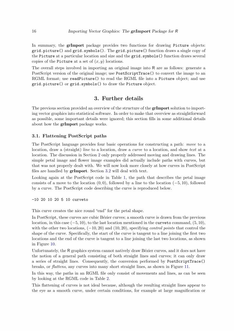
The PostScript language provides four basic operations for constructing a path: move to alocation, draw a (straight) line to a location, draw a curve to a location, and show text at alocation. The discussion in Section 2 only properly addressed moving and drawing lines. Thesimple petal image and flower image examples did actually include paths with curves, butthat was not properly dealt with. We will now look more closely at how curves in PostScriptfiles are handled by grImport. Section 3.2 will deal with text.
Looking again at the PostScript code in Table 1, the path that describes the petal imageconsists of a move to the location (0, 0), followed by a line to the location (−5, 10), followedby a curve. The PostScript code describing the curve is reproduced below.
-10 20 10 20 5 10 curveto
This curve creates the nice round “end” for the petal shape.
In PostScript, these curves are cubic Bezier curves; a smooth curve is drawn from the previouslocation, in this case (−5, 10), to the last location mentioned in the curveto command, (5, 10),with the other two locations, (−10, 20) and (10, 20), specifying control points that control theshape of the curve. Specifically, the start of the curve is tangent to a line joining the first twolocations and the end of the curve is tangent to a line joining the last two locations, as shownin Figure 10.
Unfortunately, the R graphics system cannot natively draw Bezier curves, and it does not havethe notion of a general path consisting of both straight lines and curves; it can only drawa series of straight lines. Consequently, the conversion performed by PostScriptTrace()breaks, or flattens, any curves into many short straight lines, as shown in Figure 11.
In this way, the paths in an RGML file only consist of movements and lines, as can be seenby looking at the RGML code in Table 2.
This flattening of curves is not ideal because, although the resulting straight lines appear tothe eye as a smooth curve, under certain conditions, for example at large magnification or
Journal of Statistical Software 17
●
● ●
●(−5, 10)
(−10, 20) (10, 20)
(5, 10)
Figure 10: An illustration of how a bezier curve is drawn relative to four control points.
●
● ●
●(−5, 10)
(−10, 20) (10, 20)
(5, 10)●●
●
●
●
●
●●
●●●●
●
●
●
●
●
●
Figure 11: An illustration of how the import process “flattens” a bezier curve into a series ofstraight lines.
when lines are very thick, the corners where the straight lines meet can become noticeable.Because of this, PostScriptTrace() has an argument called setflat, which controls howmany straight lines the curve is broken into. Larger values (up to a maximum of 100) resultin fewer straight lines and smaller values (down to a minimum of 0.2) result in more straightlines. The downside of a small value of setflat is that the RGML file will be much largerbecause there will be many more <line> elements produced.
3.2. Text
The previous section explained how PostScript curves are handled by grImport, but theability to display text in a PostScript file has been completely ignored up to this point. Thatomission is rectified in this section.
One reason for ignoring text in PostScript files is because the main focus of this article is onimporting images that are made up of shapes rather than text
Another good reason for ignoring text in PostScript files is the fact that importing text ishard. In particular it is very difficult to replicate the exact font that is used in the originalPostScript file because that information can be extremely complex.
Despite these objections, the grImport package provides two simple approaches to importingtext from a PostScript image. Neither of these approaches is ideal, but they may be betterthan nothing for certain images.
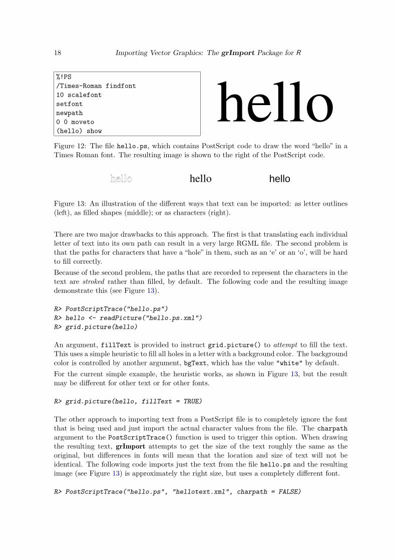
As a simple example to demonstrate these approaches, we will work with the file shown inFigure 12, which displays the word “hello” in a Times Roman font.
The first approach to importing this text into R is to convert each character in the text into(flattened) paths. The advantage of this approach is that the resulting text will look quite alot like the original text because it will be based on the actual outlines of the characters inthe original text.
18 Importing Vector Graphics: The grImport Package for R
%!PS/Times-Roman findfont10 scalefontsetfontnewpath0 0 moveto(hello) show
helloFigure 12: The file hello.ps, which contains PostScript code to draw the word “hello” in aTimes Roman font. The resulting image is shown to the right of the PostScript code.
hello
Figure 13: An illustration of the different ways that text can be imported: as letter outlines(left), as filled shapes (middle); or as characters (right).
There are two major drawbacks to this approach. The first is that translating each individualletter of text into its own path can result in a very large RGML file. The second problem isthat the paths for characters that have a “hole” in them, such as an ‘e’ or an ‘o’, will be hardto fill correctly.
Because of the second problem, the paths that are recorded to represent the characters in thetext are stroked rather than filled, by default. The following code and the resulting imagedemonstrate this (see Figure 13).
R> PostScriptTrace("hello.ps")
R> hello <- readPicture("hello.ps.xml")
R> grid.picture(hello)
An argument, fillText is provided to instruct grid.picture() to attempt to fill the text.This uses a simple heuristic to fill all holes in a letter with a background color. The backgroundcolor is controlled by another argument, bgText, which has the value "white" by default.
For the current simple example, the heuristic works, as shown in Figure 13, but the resultmay be different for other text or for other fonts.
R> grid.picture(hello, fillText = TRUE)
The other approach to importing text from a PostScript file is to completely ignore the fontthat is being used and just import the actual character values from the file. The charpathargument to the PostScriptTrace() function is used to trigger this option. When drawingthe resulting text, grImport attempts to get the size of the text roughly the same as theoriginal, but differences in fonts will mean that the location and size of text will not beidentical. The following code imports just the text from the file hello.ps and the resultingimage (see Figure 13) is approximately the right size, but uses a completely different font.
Figure 14: A modification of the flower shape from Table 3, with each petal drawn just inoutline rather than being filled.
R> hellotext <- readPicture("hellotext.xml")
R> grid.picture(hellotext)
One problem that can completely stymie attempts to import text from a PostScript file isthat some font outlines are “protected” by the font creator, which means that the font outlinecannot be converted to flattened paths, so they will resist grImport’s attempts to extractthem.
3.3. Bitmaps
As mentioned back in Section 1.2, PostScript is really a meta format rather than just avector graphics format, which means that a PostScript file can contain raster elements aswell as shapes and text. Currently, grImport will completely ignore any raster elements in aPostScript file.
3.4. Graphical parameters
The description of an image in a PostScript file consists of a description of shapes, or paths,plus a description of whether to stroke or fill each path, plus a description of what colors andline styles to use when filling or stroking each path. This section addresses the last part: howdoes grImport handle importing graphical parameters such as colors and line styles?
Whenever a path is converted from PostScript to RGML, in addition to recording the set oflocations that describe the path, PostScriptTrace() records the color, as an RGB triplet,and the line width that are used to stroke or fill the path. A minor detail is that the linewidth is scaled up by a factor of 4/3 because a line width of 1 corresponds to 1/72 inches inPostScript, but a line width of 1 corresponds to roughly 1/96 inches on R graphics devices.
By default, the colors and line widths that are recorded in the RGML file are used when draw-ing the image in R. This was vividly demonstrated on page 16 with the tiger image. However,both the grid.picture() and grid.symbols() functions provide a use.gc argument thatallows the default graphical parameters to be overridden. As a simple example, the followingcode draws just the outline of the flower image by turning off the default graphical parametersettings and specifying a transparent fill and a black border instead (see Figure 14).
R> grid.picture(PSflower, use.gc = FALSE,
+ gp = gpar(fill = NA, col = "black"))
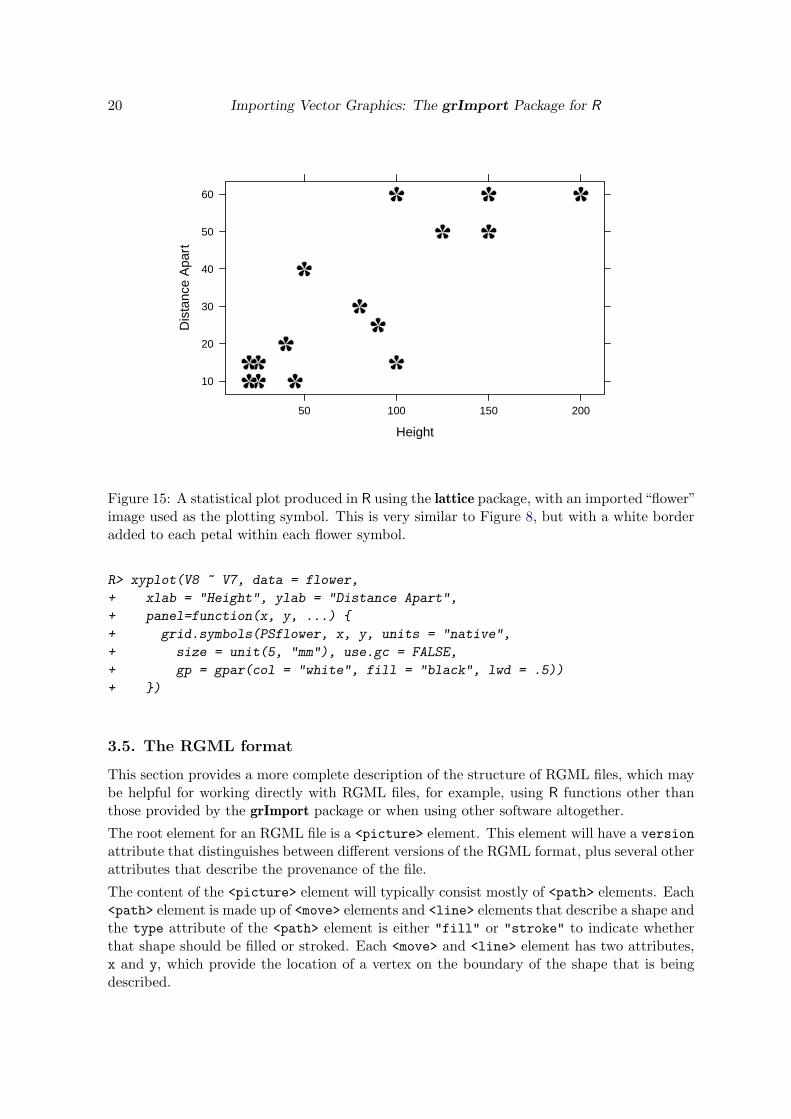
The following code demonstrates a similar usage of grid.symbols(), except in this case theblack fill has been retained and a white border has been added. This makes it is easier to seewhere flower images overlap within the plot. Figure 15 shows the resulting plot.
20 Importing Vector Graphics: The grImport Package for R
Height
Dis
tanc
e A
part
10
20
30
40
50
60
50 100 150 200
Figure 15: A statistical plot produced in R using the lattice package, with an imported“flower”image used as the plotting symbol. This is very similar to Figure 8, but with a white borderadded to each petal within each flower symbol.
R> xyplot(V8 ~ V7, data = flower,
+ xlab = "Height", ylab = "Distance Apart",
+ panel=function(x, y, ...) {
+ grid.symbols(PSflower, x, y, units = "native",
+ size = unit(5, "mm"), use.gc = FALSE,
+ gp = gpar(col = "white", fill = "black", lwd = .5))
+ })
3.5. The RGML format
This section provides a more complete description of the structure of RGML files, which maybe helpful for working directly with RGML files, for example, using R functions other thanthose provided by the grImport package or when using other software altogether.
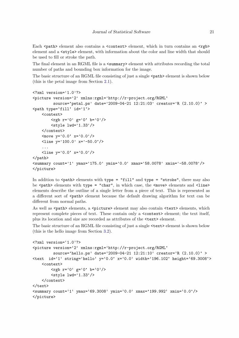
The root element for an RGML file is a <picture> element. This element will have a versionattribute that distinguishes between different versions of the RGML format, plus several otherattributes that describe the provenance of the file.
The content of the <picture> element will typically consist mostly of <path> elements. Each<path> element is made up of <move> elements and <line> elements that describe a shape andthe type attribute of the <path> element is either "fill" or "stroke" to indicate whetherthat shape should be filled or stroked. Each <move> and <line> element has two attributes,x and y, which provide the location of a vertex on the boundary of the shape that is beingdescribed.
Journal of Statistical Software 21
Each <path> element also contains a <context> element, which in turn contains an <rgb>element and a <style> element, with information about the color and line width that shouldbe used to fill or stroke the path.
The final element in an RGML file is a <summary> element with attributes recording the totalnumber of paths and bounding box information for the image.
The basic structure of an RGML file consisting of just a single <path> element is shown below(this is the petal image from Section 2.1).
In addition to <path> elements with type = "fill" and type = "stroke", there may alsobe <path> elements with type = "char", in which case, the <move> elements and <line>elements describe the outline of a single letter from a piece of text. This is represented asa different sort of <path> element because the default drawing algorithm for text can bedifferent from normal paths.
As well as <path> elements, a <picture> element may also contain <text> elements, whichrepresent complete pieces of text. These contain only a <context> element; the text itself,plus its location and size are recorded as attributes of the <text> element.
The basic structure of an RGML file consisting of just a single <text> element is shown below(this is the hello image from Section 3.2).
22 Importing Vector Graphics: The grImport Package for R
The grImport package provides a DTD file, rgml.dtd, and an equivalent XML Schema,rgml.xsd, that formalize the RGML document structure.
3.6. The Picture class
This section provides a more complete description of the Picture class, and the other asso-ciated classes, that are used to represent imported images in R. This information is useful fordealing directly with Picture objects.
As mentioned previously, the components of a Picture data structure have a one-to-onecorrespondence with the elements of an RGML file, so most elements and attributes fromthe previous section are represented as slots in an R object within this section. For example,where an RGML file has one or more <path> elements, the Picture class has a paths slotcontaining a list of paths.
A Picture object has two slots: the paths slot contains a list of shapes that describe theimage and the summary slot contains the summary information for the image.
R> slotNames(petal)
[1] "paths" "summary"
The components of the list in the paths slot are all S4 objects, each with a class correspondingto one type of <path> or <text> element in an RGML file:
RGML element S4 class<path type = "stroke"> PictureStroke<path type = "fill"> PictureFill<path type = "char"> PictureChar<text> PictureText
PictureStroke, PictureFill, and PictureChar objects all have four slots: the x and y slotscontain numeric vectors that specify the locations of the vertices of the path, an rgb slotcontains the color for the path, and an lwd slot contains the line width.
The following code and output shows the first (and only) path in the imported petal image.This path is a PictureFill object.
R> str(petal@paths[[1]])
Formal class 'PictureFill' [package "grImport"] with 4 slots..@ x : Named num [1:36] 0 -50 -54 -56.6 -57.9 ..... ..- attr(*, "names")= chr [1:36] "move" "line" "line" "line" .....@ y : Named num [1:36] 0 100 109 118 125 ..... ..- attr(*, "names")= chr [1:36] "move" "line" "line" "line" .....@ rgb: chr "#000000"..@ lwd: num 1.33
Journal of Statistical Software 23
A PictureText object has three additional slots: the string slot contains the text to draw,and the w and h slots contain the width and height of the text, respectively.
The following code and output shows the first (and only) path in the imported text image.This path is a PictureText object.
R> str(hellotext@paths[[1]])
Formal class 'PictureText' [package "grImport"] with 7 slots..@ string: Named chr "hello".. ..- attr(*, "names")= chr "string"..@ w : num 196..@ h : num 69.3..@ x : num 0..@ y : num 0..@ rgb : chr "#000000"..@ lwd : num 1.33
The summary slot of a Picture object is a PictureSummary object with slots for the numberof shapes in the image, plus bounding box information. The following code and output showsthe summary information from the imported petal image.
R> str(petal@summary)
Formal class 'PictureSummary' [package "grImport"] with 3 slots..@ numPaths: Named num 1.. ..- attr(*, "names")= chr "count"..@ xscale : Named num [1:2] -58 58.. ..- attr(*, "names")= chr [1:2] "xmin" "xmax"..@ yscale : Named num [1:2] 0 175.. ..- attr(*, "names")= chr [1:2] "ymin" "ymax"
3.7. Picture objects to grid grobs
The grid.picture() function uses the grid package to draw a Picture object.
This involves two steps: first the Picture object is converted into several grid grobs (graphicalobjects) and then those grobs are drawn within a grid viewport that takes care of all of thenecessary coordinate system transformations.
The grid.picture() function converts a Picture object to grobs by calling the functiongrobify() on each component of the paths slot in the Picture object. The grobify() func-tion is an S4 generic function with methods for PictureFill, PictureStroke, PictureChar,and PictureText objects. For example, the grobify() method for PictureFill objectscreates a polygon grob, whereas the method for PictureText objects creates a text grob.
The grid.picture() function provides an argument called FUN that allows the grobify()function to be replaced with a custom function. This makes it possible to fully control theconversion of the Picture paths into grid grobs.
24 Importing Vector Graphics: The grImport Package for R
rgb <- col2rgb(inrgb)RGB <- RGB(t(rgb)/255)# Special case "black"if (all(coords(RGB) == 0))
RGB <- RGB(0, 0, .1)LCH <- as(RGB, "polarLUV")lch <- coords(LCH)# Scale the chroma so greys become blueshcl(240, 20 + .8*lch[2], lch[1])
}
Table 6: R code that defines a function to convert an RGB color into a corresponding shadeof blue.
Table 7 shows an example of this sort of customization. An S4 generic function calledblueify() is defined, with methods for PictureFill and PictureStroke objects. ThePictureFill method produces a polygon grob and the PictureStroke method producesa polyline grob, just like the standard grobify() function would do. The difference is thatthe blueify() methods set the fill and border colors for these grobs by converting the orig-inal RGB color from the the original image to a corresponding shade of blue (using theblueShade() function that is defined in Table 6).
With this blueify() generic function defined, we can draw the tiger image that we saw onpage 16, but this time using different shades of blue. The following code does this drawingand the resulting image is shown in Figure 16.
R> grid.picture(tiger[-1], FUN = blueify)
3.8. Complex paths
One of the more sophisticated features of PostScript is that it allows paths to be quite complex.For example, a path may intersect itself and a path may be disjoint, being composed of morethan one shape, with the shapes able to overlap and create holes within one another. Thiscan create a problem for importing such an image to R because R graphics cannot draw suchcomplex paths.
In order to demonstrate these ideas, the next example introduces a new image, which is alogo for the GNU project (designed by Aurelio A. Heckert). The original file is in an SVGformat and this was converted to a PostScript format using Inkscape. The PostScript file,GNU.ps, can be imported using the tools described previously, as shown by the following code.However, the result is not quite right.
Table 7: R code that defines a custom transformation from Picture paths to grid grobs.The function blueify() is an S4 generic function with methods for PictureFill andPictureStroke objects. This function generates grobs that have a fill color or border colorbased on the original colors from the image, but converted into a corresponding shade of blue,using the blueShade() function from Table 6.
Figure 16: A modification of the tiger image from Figure 9 with all colors drawn as shades ofblue.
26 Importing Vector Graphics: The grImport Package for R
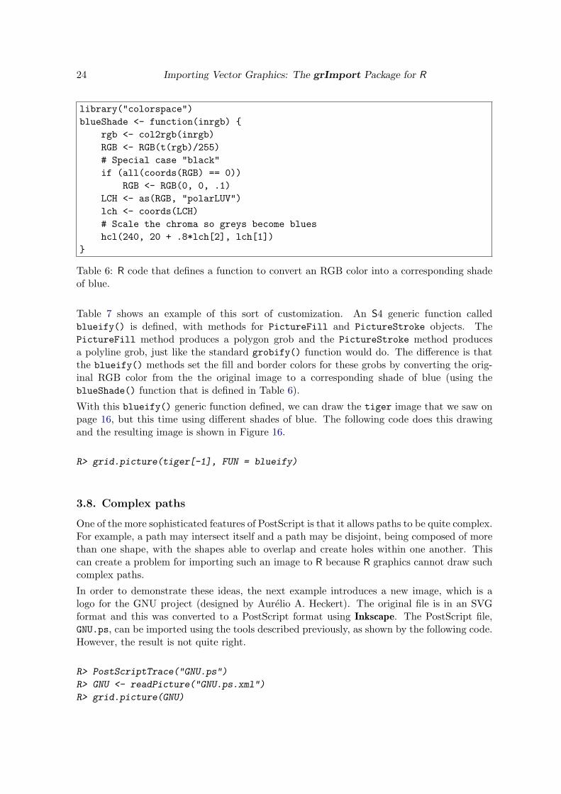
Figure 17: The original GNU logo (left), the default image after importing and drawing withR (middle), and a zoomed view of the problem area with R’s version (right).
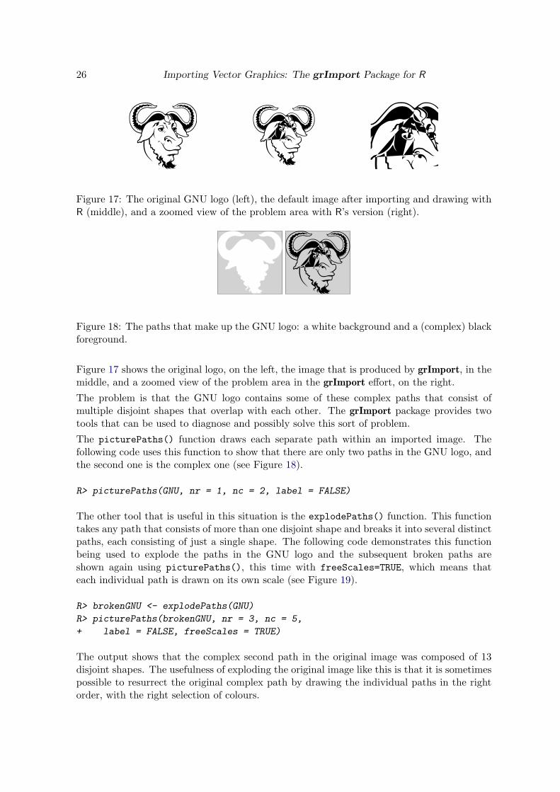
Figure 18: The paths that make up the GNU logo: a white background and a (complex) blackforeground.
Figure 17 shows the original logo, on the left, the image that is produced by grImport, in themiddle, and a zoomed view of the problem area in the grImport effort, on the right.
The problem is that the GNU logo contains some of these complex paths that consist ofmultiple disjoint shapes that overlap with each other. The grImport package provides twotools that can be used to diagnose and possibly solve this sort of problem.
The picturePaths() function draws each separate path within an imported image. Thefollowing code uses this function to show that there are only two paths in the GNU logo, andthe second one is the complex one (see Figure 18).
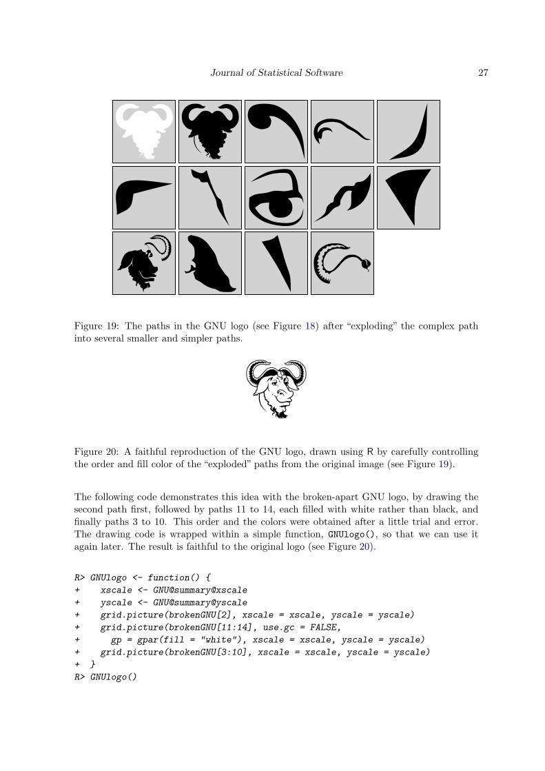
The other tool that is useful in this situation is the explodePaths() function. This functiontakes any path that consists of more than one disjoint shape and breaks it into several distinctpaths, each consisting of just a single shape. The following code demonstrates this functionbeing used to explode the paths in the GNU logo and the subsequent broken paths areshown again using picturePaths(), this time with freeScales=TRUE, which means thateach individual path is drawn on its own scale (see Figure 19).
R> brokenGNU <- explodePaths(GNU)
R> picturePaths(brokenGNU, nr = 3, nc = 5,
+ label = FALSE, freeScales = TRUE)
The output shows that the complex second path in the original image was composed of 13disjoint shapes. The usefulness of exploding the original image like this is that it is sometimespossible to resurrect the original complex path by drawing the individual paths in the rightorder, with the right selection of colours.
Journal of Statistical Software 27
Figure 19: The paths in the GNU logo (see Figure 18) after “exploding” the complex pathinto several smaller and simpler paths.
Figure 20: A faithful reproduction of the GNU logo, drawn using R by carefully controllingthe order and fill color of the “exploded” paths from the original image (see Figure 19).
The following code demonstrates this idea with the broken-apart GNU logo, by drawing thesecond path first, followed by paths 11 to 14, each filled with white rather than black, andfinally paths 3 to 10. This order and the colors were obtained after a little trial and error.The drawing code is wrapped within a simple function, GNUlogo(), so that we can use itagain later. The result is faithful to the original logo (see Figure 20).
28 Importing Vector Graphics: The grImport Package for R
4. Applications and examples
This section describes and demonstrates some possible uses of the grImport package.
A straightforward use of the grid.symbols() function is to import an external image as acustom plotting symbol for a scatterplot, as was previously demonstrated in Figure 8 (Sec-tion 2.3).
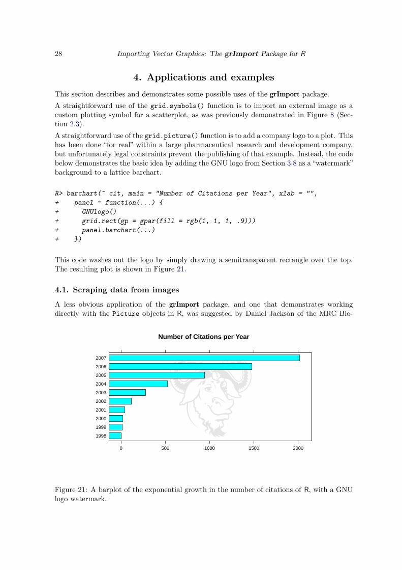
A straightforward use of the grid.picture() function is to add a company logo to a plot. Thishas been done “for real” within a large pharmaceutical research and development company,but unfortunately legal constraints prevent the publishing of that example. Instead, the codebelow demonstrates the basic idea by adding the GNU logo from Section 3.8 as a “watermark”background to a lattice barchart.
R> barchart(~ cit, main = "Number of Citations per Year", xlab = "",
+ panel = function(...) {
+ GNUlogo()
+ grid.rect(gp = gpar(fill = rgb(1, 1, 1, .9)))
+ panel.barchart(...)
+ })
This code washes out the logo by simply drawing a semitransparent rectangle over the top.The resulting plot is shown in Figure 21.
4.1. Scraping data from images
A less obvious application of the grImport package, and one that demonstrates workingdirectly with the Picture objects in R, was suggested by Daniel Jackson of the MRC Bio-
Number of Citations per Year
1998
1999
2000
2001
2002
2003
2004
2005
2006
2007
0 500 1000 1500 2000
Figure 21: A barplot of the exponential growth in the number of citations of R, with a GNUlogo watermark.
Journal of Statistical Software 29
statistics Unit in Cambridge (private communication). The context for this application is thepractice of meta-analysis, specifically in the area of survival data.
A problem that researchers face in this area is how to obtain data from published articles whenthe original data are not provided. An article may include summary tables and plots, butraw data values may not be available. In practice, researchers sometimes resort to measuringplots, such as survival curves, with a pencil and ruler in order to retrieve at least some rawdata points. If an article of interest is published in an electronic format, it may be possibleto use the grImport package to radically improve both the accuracy and efficiency of such atask.
In order to demonstrate this idea, the following example will process a survival curve thatwas published in the newsletter of the R project for statistical computing (Lumley 2004).
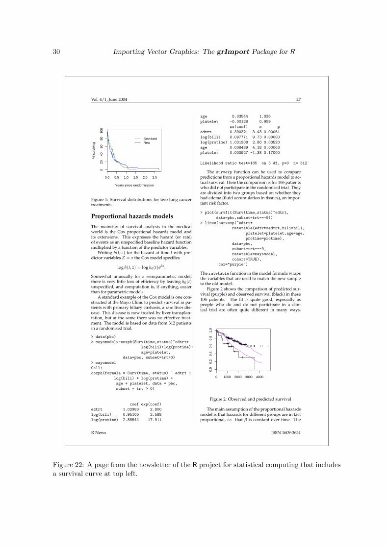
A survival plot appears on page 27 of this R News issue. Figure 22 shows the original contextof the plot.
A number of tools can be used to extract just a single page from a multiple-page PDFdocument and convert that page to PostScript format. In this case, the resulting file is calledpage27.ps and this is converted to RGML format by the following code.
R> PostScriptTrace("page27.ps")
We do not need the entire page, but using the picturePaths() function and a little trial anderror, it is possible to determine which paths constitute the survival plot in the top-left cornerof the page. The following code reads the RGML file into a Picture object and extracts justthe paths that make up the crucial part of the plot: paths 3 to 16 draw the axes, path 18 isthe green curve, and path 27 is the blue curve.
R> page27 <- readPicture("page27.ps.xml")
R> survivalPlot <- page27[c(3:16, 18, 27)]
The following code draws the extracted paths and the result is shown in Figure 23.
R> pushViewport(viewport(gp = gpar(lex = .2)))
R> grid.picture(survivalPlot)
R> popViewport()
The original image shows that the outer tick marks are at locations 0 and 100 on the y-axisand 0 and 2.5 on the x-axis. These locations can be matched to the locations of the pathsthat make up those tick marks in the Picture object in order to establish a scale for thepaths that make up the green and blue curves. For example, the picturePaths() functioncan be used to determine that the lowest tick mark on the y-axis is drawn by the ninth pathin survivalPlot and zero on the vertical scale is at the y-location of this path.
R> zeroY <- survivalPlot@paths[[9]]@y[1]
R> zeroY
move6308.73
30 Importing Vector Graphics: The grImport Package for R
Vol. 4/1, June 2004 27
0.0 0.5 1.0 1.5 2.0 2.5
020
4060
8010
0
Years since randomisation
% s
urvi
ving
StandardNew
Figure 1: Survival distributions for two lung cancertreatments
Proportional hazards models
The mainstay of survival analysis in the medicalworld is the Cox proportional hazards model andits extensions. This expresses the hazard (or rate)of events as an unspecified baseline hazard functionmultiplied by a function of the predictor variables.
Writing h(t; z) for the hazard at time t with pre-dictor variables Z = z the Cox model specifies
log h(t, z) = log h0(t)eβz.
Somewhat unusually for a semiparametric model,there is very little loss of efficiency by leaving h0(t)unspecified, and computation is, if anything, easierthan for parametric models.
A standard example of the Cox model is one con-structed at the Mayo Clinic to predict survival in pa-tients with primary biliary cirrhosis, a rare liver dis-ease. This disease is now treated by liver transplan-tation, but at the same there was no effective treat-ment. The model is based on data from 312 patientsin a randomised trial.
The survexp function can be used to comparepredictions from a proportional hazards model to ac-tual survival. Here the comparison is for 106 patientswho did not participate in the randomised trial. Theyare divided into two groups based on whether theyhad edema (fluid accumulation in tissues), an impor-tant risk factor.
The ratetable function in the model formula wrapsthe variables that are used to match the new sampleto the old model.
Figure 2 shows the comparison of predicted sur-vival (purple) and observed survival (black) in these106 patients. The fit is quite good, especially aspeople who do and do not participate in a clin-ical trial are often quite different in many ways.
0 1000 2000 3000 4000
0.0
0.2
0.4
0.6
0.8
1.0
Figure 2: Observed and predicted survival
The main assumption of the proportional hazardsmodel is that hazards for different groups are in factproportional, i.e. that β is constant over time. The
R News ISSN 1609-3631
Figure 22: A page from the newsletter of the R project for statistical computing that includesa survival curve at top left.
Journal of Statistical Software 31
Figure 23: The survival plot from the R News article, which is drawn by importing the originalpage and subsetting the relevant paths from that page.
Similarly, the uppermost tick mark is path 14, so a unit step on the vertical scale is 1100th of
the difference between the y-location of this path and that of path 9.
The survival percentages from the green curve (path 15 of survivalPlot) can now be de-termined using this scale information. Each y-value repeats twice because the green curve isdrawn as a step function.
Happily, these numbers match quite well with the values that were used to produce the originalplot.
R> library("survival")
R> sfit <- survfit(Surv(time, status) ~ trt, data = veteran)
R> originalGreenY <- sfit$surv[1:sfit$strata[1]]
R> head(round(originalGreenY*100, 1), n = 9)
[1] 98.6 97.1 95.7 92.8 89.9 88.4 85.5 84.1 82.6
32 Importing Vector Graphics: The grImport Package for R
Figure 24: An example of a sequence logo produced by the WebLogo software.
The x-values for the green curve and the data from the blue curve could be extracted in ananalogous fashion.
This idea of importing images just to extract the locations from the boundaries of shapes inthe image might also be usefully applied to map data that is only available in pictorial form.
4.2. Importing WebLogo images
The next example demonstrates a more sophisticated use of grid.picture() based on workby Toby Dylan Hocking (http://www.ocf.berkeley.edu/~tdhock/). The images to be im-ported are sequence logos (Schneider and Stephens 1990) as generated by the WebLogo soft-ware (Crooks, Hon, Chandonia, and Brenner 2004, http://weblogo.berkeley.edu/).
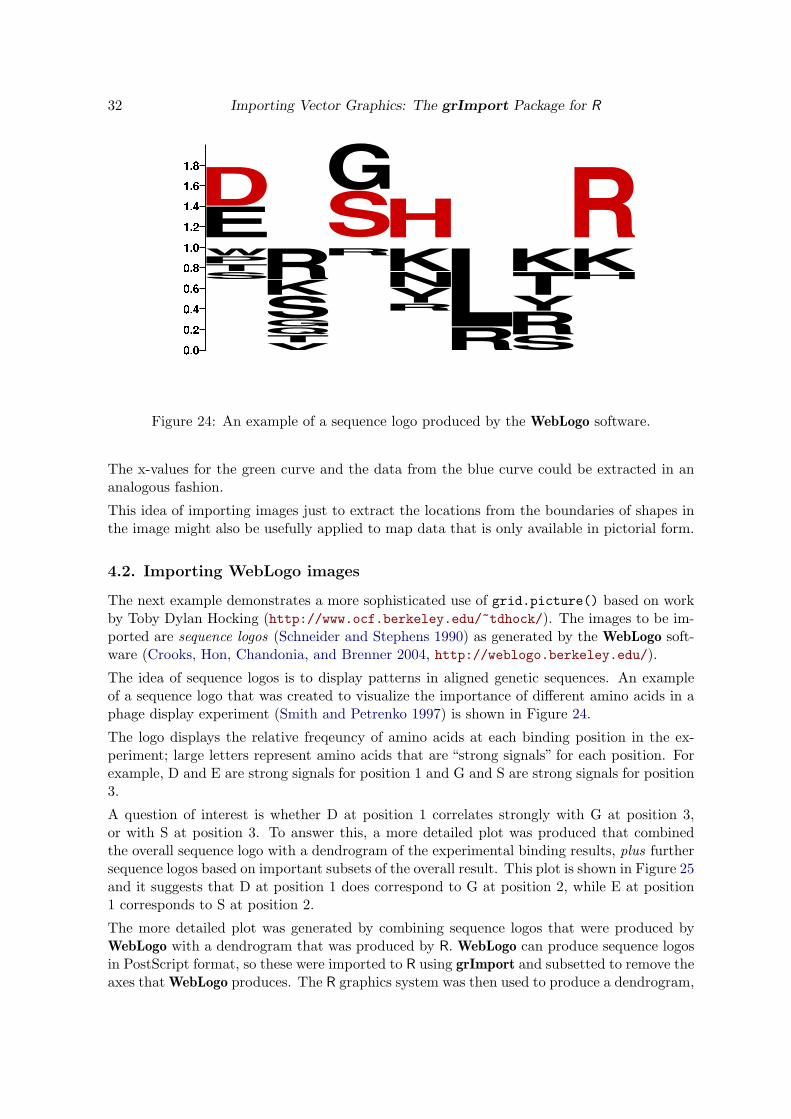
The idea of sequence logos is to display patterns in aligned genetic sequences. An exampleof a sequence logo that was created to visualize the importance of different amino acids in aphage display experiment (Smith and Petrenko 1997) is shown in Figure 24.
The logo displays the relative freqeuncy of amino acids at each binding position in the ex-periment; large letters represent amino acids that are “strong signals” for each position. Forexample, D and E are strong signals for position 1 and G and S are strong signals for position3.
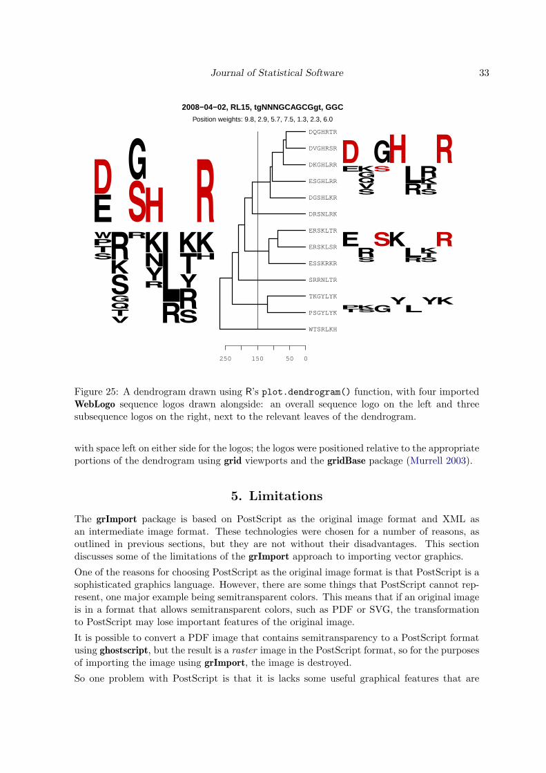
A question of interest is whether D at position 1 correlates strongly with G at position 3,or with S at position 3. To answer this, a more detailed plot was produced that combinedthe overall sequence logo with a dendrogram of the experimental binding results, plus furthersequence logos based on important subsets of the overall result. This plot is shown in Figure 25and it suggests that D at position 1 does correspond to G at position 2, while E at position1 corresponds to S at position 2.
The more detailed plot was generated by combining sequence logos that were produced byWebLogo with a dendrogram that was produced by R. WebLogo can produce sequence logosin PostScript format, so these were imported to R using grImport and subsetted to remove theaxes that WebLogo produces. The R graphics system was then used to produce a dendrogram,
Position weights: 9.8, 2.9, 5.7, 7.5, 1.3, 2.3, 6.0
Figure 25: A dendrogram drawn using R’s plot.dendrogram() function, with four importedWebLogo sequence logos drawn alongside: an overall sequence logo on the left and threesubsequence logos on the right, next to the relevant leaves of the dendrogram.
with space left on either side for the logos; the logos were positioned relative to the appropriateportions of the dendrogram using grid viewports and the gridBase package (Murrell 2003).
5. Limitations
The grImport package is based on PostScript as the original image format and XML asan intermediate image format. These technologies were chosen for a number of reasons, asoutlined in previous sections, but they are not without their disadvantages. This sectiondiscusses some of the limitations of the grImport approach to importing vector graphics.
One of the reasons for choosing PostScript as the original image format is that PostScript is asophisticated graphics language. However, there are some things that PostScript cannot rep-resent, one major example being semitransparent colors. This means that if an original imageis in a format that allows semitransparent colors, such as PDF or SVG, the transformationto PostScript may lose important features of the original image.
It is possible to convert a PDF image that contains semitransparency to a PostScript formatusing ghostscript, but the result is a raster image in the PostScript format, so for the purposesof importing the image using grImport, the image is destroyed.
So one problem with PostScript is that it is lacks some useful graphical features that are
34 Importing Vector Graphics: The grImport Package for R
Figure 26: An example of complex clipping: the pattern on the left is clipped to the shape ofthe text “hello” on the right.
eofill fill
Figure 27: An illustration of the difference between the non-zero winding rule (right) and theeven-odd rule (left) for filling the same polygon.
available in other vector formats. A different problem with using PostScript is that it pos-sesses some useful graphical features that R graphics lacks. An example of this problemwas discussed in Section 3.8; a PostScript path can be more complex than R is capable ofdrawing. Previous sections have also mentioned that a PostScript file can contain raster ele-ments, which grImport just ignores, and Bezier curves, which grImport flattens into a seriesof straight lines.
Some other PostScript features that are not supported by either R graphics in general orgrImport specifically are:
Clipping to arbitrary paths: PostScript allows clipping to the current path, which can bea very complex shape. As a simple example, the image in Figure 26 shows a pattern ofradiating lines on the left; the image on the right in Figure 26 shows this pattern beingclipped to the outline of a piece of text.
R graphics only allows clipping to a rectangle and grImport currently completely ignoresany clipping in a PostScript image, so an original image that makes uses of clipping canbe imported but will not be reproduced correctly in R.
The path fill rule: When a self-intersecting path is filled with a color, there are two mainways to decide what constitutes the “inside” of the resulting shape. The two algorithmsare called the non-zero winding rule and the even-odd rule. The image in Figure 27demonstrates the difference by showing exactly the same (self-intersecting) path beingfilled with the two algorithms (the even-odd rule is on the left).
PostScript can perform either type of fill, but R graphics only uses the non-zero windingrule, so an original PostScript image that uses the even-odd rule can be imported, butit will not reproduce correctly in R.
Moving on to the choice of XML as an intermediate format, the main problem is that XMLis a verbose language that can result in large files. However, this problem has so far provento be an inconvenience rather than an insurmountable obstacle.
Journal of Statistical Software 35
6. Availability
The grImport package is available from the Comprehensive R Archive Network (R Foundationfor Statistical Computing 2008) at http://CRAN.R-project.org/package=grImport. Thisarticle describes version 0.4-3 of the package.
7. Conclusion
The grImport package implements a three-stage approach to importing vector-based graphicalimages into the R software environment for statistical computing and graphics.
It is assumed that the original image can be converted to a PostScript format, then functionsin the grImport package are provided to convert the PostScript file to an intermediate RGMLformat, to read the RGML file into S4 objects in R, and to manipulate and draw those objects.
There are limitations to the system, due to the limitations of the PostScript language anddue to the limitations of the R graphics system, although some of these issues can be workedaround. Furthermore, despite these limitations, the grImport package has been employed ina variety of ways in several real-world applications.
One of the important ideas to take away is that the grImport package is not just aboutdrawing pictures. The package starts with a vector image and transforms the image intodata. One of the things that can be done with data in R is to draw it, but there are manyother potential applications for the image data.
Acknowledgments
Richard Walton made contributions to the grImport package during a Faculty of Sciencesummer scholarship at the University of Auckland (2005/2006).
Thanks to the authors of the freely-available images that are used in this article. The chesspawn is from a public domain chess board image in SVG format by Jose Hevia, whichwas originally sourced from the Open Clip Art Library http://openclipart.org/clipart//recreation/games/chess/chess_game_01.svg, but is now available from http://www.public-domain-photos.com/free-cliparts/other/chess/chess_game_01-3657.htm. TheGNU logo is by Aurelio A. Heckert and is available from http://commons.wikimedia.org/wiki/Image:Heckert_GNU_white.svg under a Free Art Licence. The tiger image is dis-tributed as part of the ghostscript software system.
Thanks also for ideas and data to Toby Dylan Hocking and Daniel Jackson. The R citationdata used in Figure 21 were taken from an email to the R-help mailing list by John Maindonald.
Comments and suggestions from the anonymous reviewers were extremely useful in focusingand improving the final manuscript.
References
Adobe Systems (1999). Postscript Language Reference. 3rd edition. Addison-Wesley. ISBN9780201379228.
36 Importing Vector Graphics: The grImport Package for R
Adobe Systems (2005). PDF Reference Version 1.6. 5th edition. Adobe Press. ISBN9780321304742.
Bah T (2007). Inkscape: Guide to a Vector Drawing Program. Prentice Hall Press, UpperSaddle River, NJ, USA. ISBN 9780131357945.
Bivand R, Leisch F, Maechler M (2008). pixmap: Bitmap Images (“Pixel Maps”). R packageversion 0.4-9, URL http://CRAN.R-project.org/package=pixmap.
Bray T, Paoli J, Sperberg-McQueen CM, Maler E, Yergeau F (2006). Extensible MarkupLanguage (XML) 1.0. World Wide Web Consortium (W3C). URL http://www.w3.org/TR/2006/REC-xml-20060816/.
Clark J (1999). XSL Transformations (XSLT). World Wide Web Consortium (W3C). URLhttp://www.w3.org/TR/xslt/.
Crooks GE, Hon G, Chandonia JM, Brenner SE (2004). “WebLogo: A Sequence Logo Gen-erator.” Genome Research, 14, 1188–1190.
Ferraiolo J, Jun F, Jackson D (2003). Scalable Vector Graphics (SVG) 1.1 Specification. WorldWide Web Consortium (W3C). URL http://www.w3.org/TR/SVG11/.
Kylander OS, Kylander K (1999). GIMP: The Official Handbook. Coriolis Value. ISBN1576105202.
Lumley T (2004). “The survival Package.” R News, 4(1), 26–28. URL http://CRAN.R-project.org/doc/Rnews/.
Merz T (1997). Ghostscript User Manual. URL ftp://mirror.cs.wisc.edu/pub/mirrors/ghost/gs5man_e.pdf.
Murrell P (2003). “Integrating grid Graphics Output with Base Graphics Output.” R News,3(2), 7–12. URL http://CRAN.R-project.org/doc/Rnews/.
Murrell P (2005). R Graphics. Chapman & Hall/CRC, Boca Raton, FL. ISBN 1-584-88486-X,URL http://www.stat.auckland.ac.nz/~paul/RGraphics/rgraphics.html.
Nikon Systems Inc (2005). rimage: Image Processing Module for R. R package version 0.5-7,URL http://CRAN.R-project.org/package=rimage.
R Development Core Team (2008). R: A Language and Environment for Statistical Computing.R Foundation for Statistical Computing, Vienna, Austria. ISBN 3-900051-07-0, URL http://www.R-project.org/.
R Foundation for Statistical Computing (2008). Comprehensive R Archive Network. URLhttp://CRAN.R-project.org/.
Sarkar D (2008). lattice: Multivariate Data Visualization with R. Springer-Verlag, New York.ISBN 9780387759685.
Schneider TD, Stephens RM (1990). “Sequence Logos: A New Way to Display ConsensusSequences.” Nucleic Acids Res, 18, 6097–6100.
Sklyar O, Huber W (2006). “Image Analysis for Microscopy Screens.” R News, 6(5), 12–16.URL http://CRAN.R-project.org/doc/Rnews/.
Smith GP, Petrenko VA (1997). “Phage Display.” Chemical Reviews, 97(2), 391–410.
Still M (2005). The Definitive Guide to ImageMagick. Apress. ISBN 9781590595909.
Temple Lang D (2008). XML: Tools for Parsing and Generating XML Within R and S-PLUS.R package version 1.95-3, URL http://CRAN.R-project.org/package=XML.
Veillard D (2009). “The XSLT C Library for GNOME.” http://xmlsoft.org/XSLT/.
Affiliation:
Paul MurrellDepartment of StatisticsThe University of AucklandPrivate Bag 92019Auckland, New ZealandTelephone: +64/9/3737599-85392E-mail: [email protected]: http://www.stat.auckland.ac.nz/~paul/
Journal of Statistical Software http://www.jstatsoft.org/published by the American Statistical Association http://www.amstat.org/