Imports in the Washington State Economy: Importance and Regional Effects of Import Liberalization 1 Christine Wieck 2 and Thomas I. Wahl IMPACT Center and School of Economic Sciences, Washington State University Pullman, WA Selected Paper/Poster American Agricultural Economics Association Portland, Oregon, July 29 - August 1, 2007 Abstract This paper focuses on the import side of a regional economy quantifying the economic impact of import levels and trade liberalization. An innovation represents the linkage of a regional with a national model by combining two separate Computable General Equilibrium models into one framework. This allows for import price formation in liberalization scenarios on the national level and subsequent incorporation of these nationally simulated prices into the regional model. The regional model is applied to Washington State, one of the most trade dependent states of the U.S, the national model to the U.S. Data for the two identically structured models origin from the IMPLAN database which divides the U.S. and Washington economy into 509 industries. For both models, Monte Carlo techniques are used to mitigate parameter uncertainty inherent in CGE specifications. Two scenarios are simulated that differ in the assumptions about the macroeconomic and factor market adjustment options of the economies. Keywords: Computable General equilibrium, regional modelling, trade liberalization JEL classification: C68, R13, F17 1 Copyright 2007 by Christine Wieck and Thomas I. Wahl. All rights reserved. The authors gratefully acknowledge helpful comments and suggestions by Dr. David Holland, Washington State University. 2 Corresponding author: Christine Wieck ([email protected]) 1
Transcript
Imports in the Washington State Economy: Importance and Regional Effects of Import Liberalization1
Christine Wieck2 and Thomas I. Wahl
IMPACT Center and School of Economic Sciences, Washington State University
Pullman, WA
Selected Paper/Poster
American Agricultural Economics Association
Portland, Oregon, July 29 - August 1, 2007
Abstract This paper focuses on the import side of a regional economy quantifying the economic impact of import levels and trade liberalization. An innovation represents the linkage of a regional with a national model by combining two separate Computable General Equilibrium models into one framework. This allows for import price formation in liberalization scenarios on the national level and subsequent incorporation of these nationally simulated prices into the regional model.
The regional model is applied to Washington State, one of the most trade dependent states of the U.S, the national model to the U.S. Data for the two identically structured models origin from the IMPLAN database which divides the U.S. and Washington economy into 509 industries. For both models, Monte Carlo techniques are used to mitigate parameter uncertainty inherent in CGE specifications. Two scenarios are simulated that differ in the assumptions about the macroeconomic and factor market adjustment options of the economies.
Keywords: Computable General equilibrium, regional modelling, trade liberalization
JEL classification: C68, R13, F17
1 Copyright 2007 by Christine Wieck and Thomas I. Wahl. All rights reserved. The authors gratefully acknowledge helpful comments and suggestions by Dr. David Holland, Washington State University. 2 Corresponding author: Christine Wieck ([email protected])
The trend towards more integrated economies that depend on the international exchange
of goods has been accelerated over the past decades. Between 1980 and 1998, the
worldwide trade volume increased at an average annual growth rate of 5.6%, much
higher than the 3.3% growth rate for global production (OFM, 2000). Washington State is
one of the most trade dependent states of the U.S., consistently ranking in the top five
states in exports during the last decade (OFM, 2005). Due to its geographical location,
Washington State serves as one of the nation’s gateways to East Asia. The ports of
Tacoma and Seattle are the second largest container load centers in the U.S., ahead of
New York/New Jersey and second only to Los Angeles/Long Beach (WITC 2003). The
value of imports and exports that were processed through the port system of Washington
State continuously increased over the past decade and accounted for $98 billion in the
year 2003 (Figure 1).
Figure 1 Value of imports and exports (“Pass-through”)
Washington State
010,00020,00030,00040,00050,00060,00070,000
1981
1983
1985
1987
1989
1991
1993
1995
1997
1999
2001
2003
Mill
ion
$
Exports Imports
Note: All data are based on goods laded or unladed in Washington State regardless of goods origin or destination. Nominal values.Source: Department of Community, Trade and Economic Development, Washington State.
With a Gross State Product (GSP) of around $262 billion in the year 2004, Washington
State rank 14 in the U.S. in absolute terms. Important contribution to the state GSP are
provided by the real estate sector, information, manufacturing, retail and wholesale trade,
2
and the professional and technical service sectors as Figure 2 indicates. The comparison
of figures over time shows that overall contribution to the total GSP increased for the
information sector by 1.8% to 9.2% in 2004 of total state GSP, as well as the retail trade
(+1.1% to 8.2% in 2004), professional and technical services (+1.4;6.6%), and health
care sectors (+0.4;6.2%). For manufacturing we observe a decrease by -1.4% to 9.1% in
2004 as well as for the contribution of the government sectors to total GSP by around
1.8% (to 13.4% in 2004).3
Figure 2 Value added of private industries in Washington State: Development over time
0
5,000
10,000
15,000
20,000
25,000
30,000
35,000
40,000
Rea
l esta
te
Info
rmatio
n
Manu
factur
ing
Reta
il trad
e
Prof
ession
al se
rvice
s
Who
lesale
trade
Hea
lth ca
re
Finan
ce and
insu
rance
Con
struc
tion
Adm
in. +
waste
servi
ces
Tran
sport
ation
Hote
l + fo
od se
rvice
s
Othe
r serv
ices
Agri
cultu
re
Mana
gemen
t of c
ompa
nies
Utili
ties
Arts
+ rec
reatio
n
Edu
catio
nal s
ervice
s
Mill
ion
$ (r
eal)
1997 2004
Note: Real values in 2000 dollars. Source: Bureau of Economic Analysis (BEA).
In terms of employment, the statistics reveal that in 2004, manufacturing contributes to
16% of total employment and various service sectors (including government) account for
the rest. Among the service sectors, retail trade (12% in total employment), education and
health (12%), and the leisure and hospitality sector (10%) capture most of the
employment. A view on the trend shows that the importance of the service sectors
increased over time (+3.6%) on the costs of manufacturing jobs.
3 All numbers in this paragraph rely on information drawn from the BEA Regional Economic Accounts website.
3
Past bilateral, regional, and multilateral trade agreements have expanded both
export opportunities and import competition. Further future trade liberalization under the
Central American Free Trade Agreement and the Doha Round of the World Trade
Organization is expected to come and will intensify this trend. Conceptually, one may
expect that rising exports would help the state economy while rising imports would hurt
it. However, in fact, the situation is more complex affecting both manufacturing and
services, and previous studies (e.g. Chase and Pascall, 1999) indicated that also rising
imports contributed to economic growth in certain industries and that the impact of trade
liberalization will depend on the character of the regional industries.
The growth of imports over the last decade affected the regional economy both
directly and indirectly. From a consumer’s point of view, these are positive developments
given that the availability of imports increases the variety of products and services
available for purchase and may reduce their costs. On the production side, the rise of
imports can be seen both, positively and negatively. To the extent that imports are used in
the production process, an increase in availability at a potentially lower price decreases
production costs and enable the firm to remain competitive. On the negative side, imports
may have an dampening effect on the economic development of industries if they become
a new source of competition and substitute for goods and services that otherwise would
have been produced regionally. In addition, an economy like Washington State that is an
important gateway for im- and exports, benefit from increased trade volumes through all
services that are required for the processing of the shipments. Impacts of imports on
employment are most likely to fall on sectors that have a heavy component of imports as
part of total final consumption and where the industries are relevant to the regional
economy. Economic effects of these developments will include changes in production
and consumption pattern, factor valuation, employment, and state GSP.
Over the last decade, research has been done on several aspects of the importance
of foreign trade for regional economies. Recent work on determinants foreign trade
earnings is provided by Leichenko and Silva (2004) whereas several other studies
quantify the importance of imports (Chase and Pascall, 1999) or exports (Gosh and
Holland, 2004) for the regional economy and trade liberalization (Dixon et al., 2006)
using mostly input-output or Computable General Equilibrium (CGE) models.
4
Leichenko and Silva (2004) studied the effect of international trade on rural
manufacturing communities in the U.S. using a regression model where manufacturing
earnings and employment is explained by regional endowment factors, exchange rates
and indicators of regional export and import orientation. Their model suggests that the
regional impacts of trade are complex and must be differentiated for rural and urban
counties and dependent on the import or export orientation of the regional communities.
Chase and Pascall (1999) analyze the importance of imports for the Washington
State economy. First, they provide a description of trends and current situation of pass-
through trade and imports with Washington as final destination, and highlight the most
import dependent sectors and major trading partners. Afterwards, they use a model
(“Washington Input-Output model”) to estimate both, the economic impacts of pass-
through trade, i.e. all trade that is e.g. handled by the ports of Seattle and Tacoma but
further shipped to destinations mainly in the Midwest, and the economic impacts of
imports terminating in Washington State. They conclude that 7% of all employment in
Washington is import-related and that the entire trade-related employment base is around
32%.
Gosh and Holland (2004) analyze the role of agriculture and food processing
exports on the Washington economy using a social accounting matrix for 2000 that is
based on IMPLAN data. Their results indicate that there are significant indirect and
induces effects of non-agriculturally related service sectors like wholesale and retail
trade, and business, health, banking and insurance services.
Dixon et al. (2006) use a detailed U.S. CGE model to analyze the impact of the
removal of major tariffs and quotas. In addition, they implement an approach to
regionalize the national results. Using regression analysis they search for further
explanatories that beyond the regional break-down of national indicators may explain
regional differences. Their results indicate that further import liberalization would have
only small long-run effects on the U.S. economy. For most industries output changes are
in the range -/+ 1%, however there are a few industries (sugar, butter, textile) where
larger negative output changes can be expected. State employment effects are estimated
to be in the range of -0.5% to +0.2% with Idaho and North Carolina being at the negative
end of these effects and Washington State at the positive end of employment
5
developments. These state results are mainly influenced by the trade orientation of
important regional industries.
As a reason of the widespread use of input-output models and the underlying
economic base theory approach, most work in this area focused on the assessment of the
export base of a regional economy.4 However, this paper aims at expanding this picture to
the import side quantifying the economic importance of current impact levels as well as
prospects of the economy as a whole under further trade liberalization. Therefore, this
study is driven by the following research questions:
How dependent is the regional economy on imports?
What is the effect of the removal of import restraints on WA?
The analysis is undertaken using a CGE modeling framework. However, an innovation in
this approach represents the integration of the regional economy into the national picture
by combining two separate models that represent the regional economy of Washington
State and the national economy of the U.S. into one modeling framework In addition, in
both models, Monte Carlo techniques will be used in order to address parameter
uncertainty inherent in the specification of CGE models.
The remainder of the paper is organized as follows: In the next section, indicators
regarding the regional economic importance of imports are analyzed. In the third section
an import restraint liberalization scenario using CGE methodology is simulated. The last
section concludes.
2 The import picture of the regional economy
Imports of goods (or services) into an economy mainly serve two purposes: they either
enter the production chain of the regional economy as inputs in the manufacturing
process or enter the marketing or transportation chain to satisfy final consumption and
service demands by household or other institutions.5 The following graphs and tables will
4 An approach that is extended by Waters et al. (1999) including service export, extraregional income, and government transfers into the economic base estimation and related industry importance indicators. 5 This also holds for so-called “pass-through” imports that are landed at a port and then transported to a final destination that is outside of the regional economy. In this case, these imports make use of warehouse, transportation, and processing services provided by the region.
6
provide an overview on the import picture in Washington State. Year of presentation is
2003, the most recent data set available from IMPLAN (Impact Analysis for Planning)6.
2.1 Value added and employment
Overview
Table 1 provides an overview on aggregated economic indicators for Washington State as
represented in the IMPLAN database for the year 2003. Around 3.5 million jobs in
Washington State generate a value added of nearly $240 billion. Imports in the value of
$157 billion arrive in Washington State of which around $19 billion originate from
foreign destinations. Total factor return for labor (“labor earnings”) for the 3.5 million
jobs account for around $142 billion.
Table 1 Value added, employment, and imports for Washington State State aggregate ValueValue added Million $ 238,633Employment # of jobs 3,541,345Total WA imports Million $ 157,360 Foreign imports Million $ 137,455 Imports from rest of the U.S. Million $ 19,905Total labor earnings Million $ 141,662 Source: Own representation based on IMPLAN data.
Breakdown by industries
Figure 3 provides an overview on the importance of the difference industries in terms of
share in value added7 in total state value added and share of employment in total state
employment in the respective industries. While the public sectors (e.g. education,
military, waste management) accounts for both the highest value added share and
employment, other industries such as money and banking, communication also contribute
significantly to the GSP but show less importance in terms of employment. Here,
personal services (e.g. rental, legal, repair, or personal care services), other retail stores,
6 IMPLAN provides regional social accounting matrices for all counties and states of the U.S. consistent with the accounting conventions used by the BEA. 7 Value added for an industry is defined as the gross output minus intermediate inputs, i.e. it is the value added of labor and capital in that industry. The sum over all industries gives the Gross State Product, i.e. the value added of the state economy.
7
health care, construction, other business services (e.g. management and administrative
services, office support service) and hotels and restaurants also are important employers
Note: Employment in public sector: 656904. Value added share in public sector is 20%. Source: Own representation based on IMPLAN data.
In Figure 4, the same indicators are displayed but for agricultural and food related
industries. Food retail and hotel and out-of-house food services and drinking places have
by far the most importance for the state in terms of value added and employment, but all
other activities in the food production and processing sector sum up to around 136,000
employees and a value added share of around 3.5%.
8
Figure 4 Employment and value-added share for food and agricultural industries, Top 25
05000
100001500020000250003000035000400004500050000
FRETAIL
HOTREST
FORESTFRUIT
FISHF
OAGRVEGE
FROFOO
SEAFOOD
BAKERY
GREENH
CANNED
GRAIN
SOFTD
MEATPRO
BREWERY
SNACKS
OFOOD
POULTFWIN
E
POULPRO
FLMILK
SWEETS
FLOUR
DRYMLK
Empl
oym
ent
012345678
% s
hare
Employment Value Added Share
Note: Employment in food retail (FRETAIL): 185144; hotels and restaurants (HOTREST): 237230. Source: Own representation based on IMPLAN data.
2.2 The relevance of imports
Within the framework of the IMPLAN social accounting matrix (SAM), production
activities, i.e. industry sectors, produce (multiple) outputs, often called commodities.
Imports into the economy are recorded in the commodity accounts, and together with the
domestically produced output, represent the supply in the economy that can be allocated
to total domestic and export demand.8 Hence from the available data, we know the
quantity of imports of a commodity but not what it is used for in the economy
(intermediate input or final consumption). This makes some assumptions necessary in
order to come up with an estimate of the importance of imports in an economy. In the
following, the different steps of this calculation will be elaborated.
We start be looking at the import share in total consumption (Figure 5) at the
commodity level. The commodities are ranked by their share of imports. In addition, we
display the use of the good, that is, if it is mainly used as a final consumption good for
8 Here, total domestic demand (consumption) is defined as the sum of final household consumption plus intermediate use of goods. In CGE models, this total domestic demand usually further includes investment demand and government consumption. These two items are displayed in the above table but not considered in the calculations here.
9
households and institutions or as an intermediate input in the production process.9 The
display of the use of the commodity allows us to draw conclusions on the main use
imports may take in the economy and may hint at industries and consumers that will be
affected by changes in trade policy (to be further analyzed in the next section).
Figure 5 Import shares and use of commodities as final consumption good or intermediates in manufacturing, Top 25
02000400060008000
100001200014000160001800020000
FISHF
TEXTILE
MININ
G
FURNIT
AUTOM
MACHINWIN
E
ELECTR
TRANM
METALS
OILFAT
FRUIT
BREWERY
PAPERBUILD
GREENH
CANNED
OFOOD
CHEMI
SWEETS
TOBDIS
FROFOO
WOOD
FORESTVEGE
Mill
ion
dolla
rs
0
10
20
30
40
50
60
70
80
% im
port
sha
re
Final consumption Intermediate good Import share
Source: Own representation based on IMPLAN data.
Commercial fishing output, textiles, and mining show the highest import shares with
around 40%-80%. Textile products, automobiles, and furniture as well as the food and
beverage products, brewery output, canned food, sweets, tobacco and distilled items, and
frozen foods are mostly destined for the final consumption whereas for the other listed
industries intermediate use of the products in other production processes prevails (e.g.
fish commodities are mainly used as intermediate products in seafood processing as well
as the hotel and restaurant business, and as final goods in household consumption).
If we want to go one step further, and draw conclusions from the commodity
import share to the importance of imports for the industry, i.e. the production activities,
we have to make some assumptions. IMPLAN provides us with a full overview on all
inputs used in the production process of a specific commodity. We know for example that
9 Final consumption goods are defined as goods that are directly consumed by households or institutions. Intermediate goods are used as industry inputs that are accounted as inputs in the production process. Goods may serve as both, final consumption good and intermediate input. e.g. fruits and vegetables that can be consumed fresh or be used as an input in the canning industry.
10
seafood processing requires as inputs fish, other food products such as flour or fat,
construction input (building) and maintenance for the processing site, and various
business activities, just to mention a few of the inputs. Hence, if we assume that the
imports in each commodity are proportionally allocated to the various uses of the
commodity, we can add up the intermediate inputs weighted by its import shares for each
specific industry. This provides us with an estimate of the quantity of imports used in a
production processes (activities).
The next two figures disclose the share of imports in the production process
broken down to industry level. Furthermore, once we know the share of imports in the
industry, we can multiply value added generated by the industry and employment with
this industry specific import share to result in an approximation of what the contribution
of imports to the economic performance of the industry is. Hence, this calculation
assumes that the proportion of industry total cost due to imported inputs is associated
with the same proportion of value added and employment created by the industry. This
means, that e.g. employment from imports as represented in Figure 6, provides an
estimation of the number of jobs that are created due to the use of imports in the
production process.
Figure 6 Share of imports in production, employment and value added related to imports, Top 25
0500
100015002000250030003500400045005000
UTILITY
SEAFOOD
TEXTILE
CHEMI
AUTOM
MININ
G
TRANM
ELECTR
MACHINWIN
E
FURNIT
BUILD
METALS
CONST
SOFTD
BREWERY
PUBLIC
PAPER
CANNED
PERSONA
COFFEE
PROGRA
GREENHFRUIT
WOOD
Mill
ion
dolla
rs/N
umbe
r of j
obs
0.00
5.00
10.00
15.00
20.00
25.00
30.00
% s
hare
of i
mpo
rts
in in
dust
ry
Value added from imports Employment from imports Import share in industry
Note: Employment from imports: transportation equipment manufacturing: 9991; construction: 19432; public sector: 44150; personal services: 20337. Source: Own representation based on IMPLAN data.
Figure 6 shows that the highest share of imports with around 20% are used in the utilities
industry, seafood production, textile manufacturing, the chemical and automobile
11
industry. However, value added generated by imports is strongest in the public sector,
construction, and transportation equipment manufacturing. Accordingly, employment
benefits are the largest in employment centered industries such as transportation
equipment manufacturing, construction, the public sector, and personal services.
In Figure 7 the same information is displayed, but focusing on the top 25
industries in agricultural and food processing with high import shares. Besides seafood
processing, the wine industry and soft drink production show import shares that are
around 10%. A number of food and agricultural sectors provide an overall contribution to
employment, where significant value added is only generated in the seafood industry.
Figure 7 Share of imports in production, employment and value added related to imports for food and agricultural industries, Top 25
050
100150200250300350400450500
SEAFOODWIN
E
SOFTD
BREWERY
CANNED
COFFEE
GREENHFRUIT
WOOD
OFOOD
OILFAT
GRAIN
SUGARFVEGE
FROFOOOILS
ENUTS
BAKERY
SWEETS
SNACKSFISHF
ICEDES
FOREST
OAGRMill
ion
dolla
rs/N
umbe
r of j
obs
0.00
5.00
10.00
15.00
20.00
25.00
30.00
% s
hare
of i
mpo
rts
in in
dust
ry
Value added from imports Employment from imports Import share in industry
Note: Employment from imports: seafood processing: 1668; fruit industry: 1124; wood production: 929; grain production: 640. Source: Own representation based on IMPLAN data.
Summing these indicators across all industries, we are able to calculate the overall impact
of imports on the economy of Washington State (Table 2). Around 5.1% of the statewide
value added, or $12.1 billion, are supported by foreign imports. Similarly, 169,000 jobs,
4.8% of the total job base, benefits from international trade. This generates
overproportional labor earnings of approximately $7.8 billion (5.5% of total labor
earning), indicating that part of these jobs must be in the industries with higher than
12
average factor returns.10 On industry level11, we observe an average import share of about
9%. Value added generated from imports is around $202 million for the average industry,
and the average employment effect results in around 2,800 jobs and provides labor
returns of around $130 million.
Table 2 Value added, employment, and labor earnings supported by imports State aggregate ValueValue added supported by imports Million $ 12,134Share in total value added % 5.08Employment supported by imports # of jobs 168,956Share in total employment % 4.77Labor earnings supported by imports Million $ 7,776Share in total labor earnings % 5.49
Industry level ValueAverage import share % 8.78Average value added supported by imports Million $ 202Average employment supported by imports # of jobs 2,816Average labor earning supported by imports Million $ 130 Source: Own representation based on IMPLAN data.
3 The regional effects of import liberalization
In this chapter, the effects of the removal of tariffs and other import restraints on the
Washington economy will be presented. For this purpose, two CGE models, representing
the U.S. and the Washington economy are constructed and linked to each other. Next,
model, data, and scenario design will be discussed, followed by the presentation of results
for both, the U.S. and the Washington economy.
3.1 Model description for the U.S. and Washington CGE model
In order to perform the analysis, CGE models for both, the U.S. and the Washington
economy were developed that are similar to standard CGE methodology provided by 10 Compared to the estimate of about 117,000 jobs supported by imports by Chase and Pascall (1999) for 1997, import supported employment seem to have increased slightly over time. In addition, the breakdown by industry indicates a shift in sector importance. Chase and Pascall identified wholesale and retail trade as the sectors where most of the jobs were originated whereas, in the present study, most of the jobs seem to be located in the manufacturing industries. In order to further investigate this shift in size and relevance, more information on the used methodology of the Chase and Pascall study as well as consistent time series information would be necessary. 11 The 509 industries in IMPLAN for Washington State are aggregated to 65 industries in this paper.
13
Hertel (1997) or Lofgren et al. (2002). A CGE model mathematically represents the inner
working of the economy with Walrasian market clearing in all sectors. Representative
agents for producers and consumers in the various sectors apply microeconomic
behavior, i.e. maximize an objective function (profit/utility) subject to certain constraints.
All markets are interconnected and consistent. Endogenous equilibrium prices ensure that
that commodity and factor markets clear and that macroeconomic identities hold. By
Walras law, all prices and exchange rates are normalized to one in the base period. The
consumer price index (CPI) is set to be the numeraire. Because of the inter-linkages of
the sectors, shocks in any sector will seep through the economy and impact the other
sectors. Given that we use a derivative of a standard CGE model, and the basic structure
is thus familiar, in the following the specification of only some of the agents will be
briefly explained.
A linear expenditure system, generated by a Stone Geary utility function is used to
model consumer behavior where we assume utility maximization subject to a budget
constraint. We consider nine different household categories whose demand is determined
by available net income12, and several “institutional” categories (e.g. investment and
government). After allocation of the household expenditure to the different consumption
goods, an Armington specification based on a constant elasticity of substitution (CES)
function determines the composition of demand from domestically produced and
imported goods. In the Washington State model, the Armington aggregator applies to two
levels – in the first stage the substitution between domestic goods (produced in
Washington) and imported goods is allowed; in the second stage domestic imports
(imports from rest of the U.S.) and foreign imports are differentiated (imports from rest
of the world), and substitution between them may take place.
Each economy is assumed to be composed of a set of competitive industries,
where each industry uses the given endowments of primary factors of production and
intermediate inputs that are outputs of other industries, in a Leontief-cum-constant
elasticity of substitution (CES) production function to produce primary and secondary
12 Net income is defined as gross income less household savings or borrowing.
14
commodities. The Leontief part of the production function ensures “weak separability”
between primary (labor and capital) and intermediate factors.
The produced commodities can be either exported (with the same distinction as on
the import side: domestic, i.e. to the rest of the U.S., and foreign exports) or domestically
consumed with the transformation between the two being defined by a constant elasticity
of transformation (CET) function. The world price of imported goods is held constant. In
the U.S. model, the price of exported goods is derived from a constant elasticity of
demand (CED) function representing export demand of the rest of the world whereas in
the Washington State model export prices are defined exogenously (see section 3.3 for a
detailed explanation).
Choice of exogenous parameter values in the behavioral functions and the closure
rules governing this modeling system will be also discussed in the scenario description in
section 3.3. The model is implemented in levels form in the software GAMS and solved
with the PATH solver. An overview of the equation system can be found in Stodick et al.
(2004)13.
3.2 Base year social accounting matrices
For the empirical analysis, SAMs were constructed for both, the U.S. and the Washington
State model. The data in the SAM captures a detailed and consistent representation of the
economic interaction of various activities at a certain point in time. Thus, the SAM
includes the complete circular flow of all the transactions in the production, factor,
household, government and rest of the world sector. The data source of the SAM for our
economic model is the IMPLAN data base of the year 2003. IMPLAN divides the
economy into 509 industries that may be aggregated according to the needs of the
researcher. In the current application, we divide the U.S. and Washington economy into
56 sectors with special focus on the agricultural and food industries (see Appendix 6.1 for
the sectoring scheme).
Table 3 represents an overview on the base year data of the Washington SAM. As
usual for SAM accounts all industries are represented only in monetary terms and no 13 Available at: http://www.agribusiness-mgmt.wsu.edu/Holland_model/docs/Documentation.pdf.
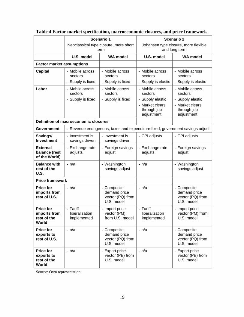
Government - Revenue endogenous, taxes and expenditure fixed, government savings adjust
Savings/ Investment
- Investment is savings driven
- Investment is savings driven
- CPI adjusts - CPI adjusts
External balance (rest of the World)
- Exchange rate adjusts
- Foreign savings adjust
- Exchange rate adjusts
- Foreign savings adjust
Balance with rest of the U.S.
- n/a - Washington savings adjust
- n/a - Washington savings adjust
Price framework
Price for imports from rest of U.S.
- n/a - Composite demand price vector (PQ) from U.S. model
- n/a - Composite demand price vector (PQ) from U.S. model
Price for imports from rest of the World
- Tariff liberalization implemented
- Import price vector (PM) from U.S. model
- Tariff liberalization implemented
- Import price vector (PM) from U.S. model
Price for exports to rest of U.S.
- n/a - Composite demand price vector (PQ) from U.S. model
- n/a - Composite demand price vector (PQ) from U.S. model
Price for exports to rest of the World
- n/a - Export price vector (PE) from U.S. model
- n/a - Export price vector (PE) from U.S. model
Source: Own representation.
19
For both scenarios hold that the current account is fixed (at the benchmark year
level) so that the foreign exchange rate fluctuates to maintain the current account balance.
Hence, depreciation or appreciation of the domestic currency unit (the dollar) may occur
in order to correct the external balance. This would simultaneously result, in the case of
depreciation, in a reduction of imports (reduction of spending) and an increase of exports
(increase export earnings). Government expenditure and investment are exogenous in the
model.
The regional open economy of Washington State is modeled in the first scenario,
as one where only short term adjustment are allowed, whereas the second scenario allows
for longer term adjustment to the changes in trade policy and represents a probably more
realistic picture. The factor market assumptions in the regional model follow U.S.
specifications. For the closure of the savings/investment balance, the state CPI is allowed
to adjust so that endogenous state savings may balance investment (fixed in real terms).
This seems a reasonable assumption in terms of regional macro behavior since there is no
mechanism to regulate the current account balance at the state level. This means that
policies or shocks at the state level that are inflationary will set off CPI changes that
reduce consumption and regulate state saving and investment. As a closure for the
external balance, the foreign exchange rate is kept fixed so that the state current account
has to adjust. This is a plausible assumption on regional level given that a regional
economy usually cannot influence foreign exchange rates. For the closure of the current
account balance with the U.S., a similar assumption is chosen where U.S. savings may
adjust.
With respect to the price framework that is relevant in the regional model, we
assume that it is determined by national market developments. Hence, in both scenarios,
national price effects of the tariff removal are estimated with the national CGE model and
these prices then are implemented and treated exogenously in the Washington model.
This step reflects the assumption that a regional economy embedded in a national context,
should face prices and macroeconomic conditions that follow national (U.S.)
developments. The endogenous market clearing implies that policy changes such as
import restraint liberalization, or movement in the exchange rate or CPI are indirectly
included in the prices. Consequently, we use the U.S. price vectors in the regional model
20
as displayed in Table 4. Different choices can be made regarding the import/export price
to and from the rest of the U.S. The national producer price (PX) can be used under the
assumption that all of Washington’s imports from the rest of the U.S. are strictly U.S.
produced. But, if some of Washington’s rest of the U.S. imports involves goods that were
originally imported from third countries, then the blended (composite) U.S. price (PQ) is
the appropriate measure. We opted for the latter one given that the U.S. in overall is a
very open economy running a trade deficit since many years.14
After the decision on model closure and exogenous elasticity values, the model is
solved initially to appropriately calibrate all the behavioral functions of the model to the
respective base year SAM. Empirical estimates of the Armington elasticities are used in
this model and are reported in Appendix 6.2 for both models. For the U.S. model, the
Armington elasticities show values in the range of 1.9-5 and result from work done by the
International Trade Commission (Donnelly et al., 2004). For the regional model, lower
substitutability is reported from empirical estimation (Bilgic et al., 2001). This reflects
the understanding that commodity imports and domestic production for a given
commodity at the national level cover more product varieties within that commodity than
is the case on a regional level. Hence, more substitution is expected among imports and
domestically produced products on the national level for a given commodity than is the
case for that same commodity at the regional level.
In order to address the uncertainty about the exogenous model parameters we
implement a sensitivity analysis based on Monte Carlo techniques as described in Abler
et al. (1999) or Gilbert (2003). The use of the Monte Carlo approach of repeated
randomized samples is only one method to systemize the uncertainty that is introduced in
the model via the parameter choices. Other possible methods include Gaussian quadrature
that approximate the underlying parameter distributions (Arndt 1996, Abler et al. 1999),
and so-called conditional (Harrison et al. 1993, Abler et al. 1999) or unconditional
systematic sensitivity analysis (Harrison and Vinod 1992, Abler et al. 1999) where only a
14 Note that in both simulations the average U.S. producer price is slightly higher than the U.S. composite price (e.g. PX=1.001% against PQ=0.997% in scenario 1) so that a small underestimation of the export effect from Washington State to the U.S. as well as a small overestimation of the import effect from the U.S. to Washington State may occur.
21
selected number of alternative values one-by-one or jointly will be tested. However,
given that these methods require either a still very high computational burden (Gaussian
quadrature) or are inferior with respect to the validity of the results, we follow Abler et al.
(1999) and Gilbert (2003) in the pragmatic approach using Monte Carlo simulation.
Elasticity of transformation between domestic (regional) and export (U.S./foreign) destination (CET)
2 1.1 – 2.9 2 1.1 – 2.9
Elasticity of transformation between rest of the U.S. and foreign destination (CET)
n/a n/a 5 2.75 – 7.25
Elasticity of substitution between domestic output and imports (Armington)
1.9 to 5.0
1.01 – 2.76 to 2.75 – 7.25
0.5 to 1.84 0.275 – 0.725 to 1.012 – 2.668
Elasticity of substitution between rest of the U.S. and foreign imports (Armington)
n/a n/a 1.9 to 5.0
1.01 – 2.76 to 2.75 – 7.25
Elasticity of demand of world export function (CED)
-2 -1.1 – 2.9 -5 -2.75 - -7.25
Income elasticity 1 0.55 – 1.45 1 0.55 – 1.45
Note: Armington elasticities are commodity specific. Source: Own compilation.
Hence, in the present study, we specify a prior distribution for the above listed
parameters, and sets of parameter values are drawn at random from these distributions
assuming that the parameters vary simultaneously and independently. We assume that
each parameter is independently normally distributed with mean values as indicated in
Table 5 and a standard deviation of 15% of the mean.15 Given that we treat the exogenous
parameters as random, all the model results subsequently are thus also random. We draw
5,000 sets of pseudo-random parameter values from their respective distribution,
15 In the choice of these values we follow Gilbert (2003). The advantage of this specification lies in the fact that virtually all variation will lie within 50% of the mean in either direction.
22
subsequently solve the model with this parameter vector, and store the simulation results.
Each outcome is an independent observation and we can estimate the expected outcome
(mean value), sensitivity of that outcome (standard deviation) and significance (t-value)
of each outcome variable.
3.4 Results
The result section is divided into two parts. First, a brief overview on the impact of tariff
reduction in the U.S. model is given. Afterwards, a more detailed presentation of the
regional impact of trade liberalization under the two different scenarios is provided. All
following tables present changes from the baseline values for selected variables. As
indicated before, all values are the mean outcomes of the respective model variables from
the 5,000 model repetitions in each scenario. Standard deviations16 for each mean
outcome are reported in italic and a star behind the variable indicates that it is
significantly different from zero at the 5% level. Most mean outcomes are robust with
respect to variation in the exogenous parameter values and only small standard deviations
of the results can be observed. This indicates that magnitude and sign of the simulated
results are rather reliable under the given model specifications. In Appendix 6.3, an
overview is given for selected variables on the variation in model variables under
different drawings from the exogenous parameter vector.
3.4.1 U.S. model
As expected, the liberalization of the trade regime in 11 of the 56 sectors brings a
stimulation of imports by around +1.1% - +1.5% for the overall U.S. economy in the two
scenarios (Table 6). Individual sector import stimulation is much higher as can be seen in
Table 7. The increased import volume slightly reduces the average price level of
composite demand (-0.002%, both scenarios) and affects total composite demand to a
small extent (-0.08% - +0.88%). This small demand decrease in the first scenario is
mainly caused by reduced savings (-2.48%) since the savings/investment balance implies
that investment demand as part of total composite demand is also moving downwards by
16 Only reported for the Washington model in this draft version.
23
around -2%. This downward movement of one component of total demand cannot be
offset by the other components of total demand that show a positive trend due to the
modest decrease in composite prices: final household consumption and demand for
intermediate goods.
Table 6 Macroeconomic and factor market changes: U.S. model
Scenario 1 Scenario 2
Savings/Investment balance
Savings -2.48% * -
CPI - 0.09% *
External balance
Exchange rate 3.09% * 3.69% *
Imports 1.11% * 1.49% *
Exports 3.15% * 4.30% *
Factor markets
Labor
Factor return 0.32% * 1.31% *
Wage rate 0.24% * -
Total employment - 1.20% * (+1,994,100 *)
Capital
Factor return 0.26% * 1.26% *
Interest rate 0.26% * 0.70% *
Total capital demand - 0.56% *
Total demand -0.08% 0.88%
GDP at market costs 0.3% * (+ $33,289 *) 1.29% * (+ $142,013 *)
Equivalent variation $18,861 * $68,525 *
Note: All values are mean outcomes from the 5000 model repetitions. Source: Own calculations.
Given the fixed external current account balance, the import increase makes an exchange
rate adjustment necessary. We observe a slight real devaluation of the domestic currency
(+3.1% - +3.7%) which induces an increase in exports by around +3.2% - +4.3%. The
sector specific effect of this exchange rate adjustment is displayed in Table 8 for the most
export dependent products. On the factor markets we observe a small increase in factor
returns. In the second scenario where total employment is allowed to adjust, we observe a
24
slight stimulation of the job market with a plus in employment of +1.2% or 1.1 million
new jobs created. These jobs are mainly created in the export oriented sectors as well as
the service industries. This positive demand for services results mainly from the increase
in equivalent variation, i.e. household income, which is with an average +$178 - $649
positive across all household categories (not presented here).
In total, the value added of the economy (GDP at market costs), is positive in both
scenarios (+0.3% - +1.3%) where the gains result mainly from increased factor returns
and household income, and a slight decrease in the composite demand price level. The
overall picture under the two macroeconomic scenarios leads to the conclusion that the
neoclassical type, short term closure allows for less adjustment of the economy to the
changes in the trade pattern compared to the more flexible specification.17
Table 7 Sectors with import restraints and the effect of reducing these: U.S. model
Next, a more detailed sector specific breakdown of the developments on the output,
import, and export side is displayed. In particular for sweet product manufacturing
(sugar) and butter processing (Table 7), the two sectors with the highest import restraints
in the benchmark, we observe a strong increase in imports that go along with a significant
output reduction. For the other products, we still observe significant import surges, but 17 Findings on exchange rate, GDP, import and export volume are quite similar to what has been simulated by Dixon et al. (2006) in a very comparable exercise with the USAGE-ITC model.
25
the impact on domestic production is less pronounced. The negative import development
for frozen food is due to the very small tariff reduction in this sector that is offset by the
increase in the exchange rate. Hence, their foreign products lose competitiveness on the
domestic market even though tariffs are reduced. In some sectors, even though higher
imports reach the domestic markets, we see output stimulation instead of the expected
output decrease. This happens in sectors that display a rather high share of exports in total
output. Their output is stimulated due to the strong export incentives introduced by the
domestic exchange rate devaluation.
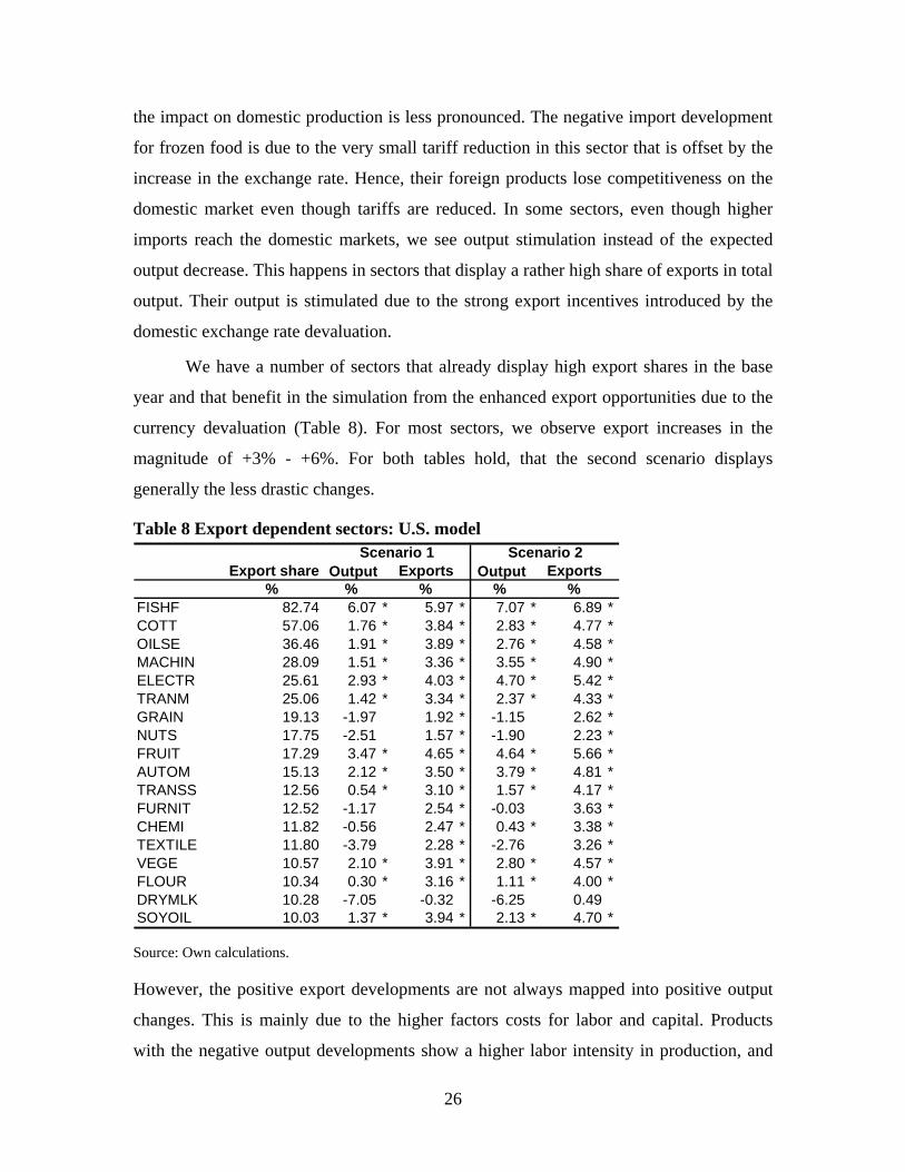
We have a number of sectors that already display high export shares in the base
year and that benefit in the simulation from the enhanced export opportunities due to the
currency devaluation (Table 8). For most sectors, we observe export increases in the
magnitude of +3% - +6%. For both tables hold, that the second scenario displays
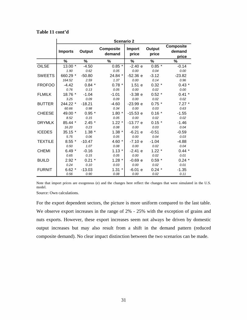
However, the positive export developments are not always mapped into positive output
changes. This is mainly due to the higher factors costs for labor and capital. Products
with the negative output developments show a higher labor intensity in production, and
26
hence they are strongly affected by the wage rate increase. This impact of increased
factor costs cannot be offset by the pull from the export market, and hence leads to a
decrease in output.
3.4.2 Washington State model
The macroeconomic variables in the Washington State model (Table 9) behave similar to
the developments observed at national level. However, trade flows show a more
pronounced reaction with imports18 in the short term model (scenario 1) increase by
around 1.7% while in the second, more flexible scenario they increase by around +2.7%.
Exports in both scenarios are stimulated by the currency deflation that took place in the
U.S. model and rise around +8.4% - +9.4%. In order to equilibrate the foreign external
balance, strong adjustments in the savings part of the balance have to be made (+140%
U.S. savings - +135% rest of the world savings). In line with the developments on
national level, demand for final consumption and intermediate inputs is slightly decreased
in the first scenario (-0.1%), whereas it increases by +1.3% in the second scenario. Even
tough we observe a slight increase in factor returns and wages and capital interests, the
household gains are apparently not strong enough in the first scenario to trigger strong
demand, and offset losses that occur in the manufacturing sectors (due to the higher
factor costs).
In total, the value added of the regional economy (GDP at market costs), is
positive in both scenarios (+0.01% - +0.04% or +$1billion - $4billion in absolute terms)
where the gains result mainly from increased factor returns and household income, and a
slight decrease in the composite demand price level.
18 In this section, the term “imports” always refer to imports from the rest of the world. If we talk about imports from rest of the U.S. this is explicitly stated.
27
Table 9 Macroeconomic and factor market changes: Washington State model Scenario 1 Scenario 2
Savings/Investment balance
Investment -3.34% (0.22) -
CPI - 0.21% * (0.02)
External balance
Foreign imports 1.71% * (0.56) 2.67% * (0.55)
Foreign exports 8.43% * (0.51) 9.39% * (0.46)
ROW savings 1.80% * (0.60) 135.14% * (6.84)
U.S. savings 140.76% * (7.68) 3.17% * (0.55)
Factor markets
Labor
Factor return 0.56% * (0.01) 1.84% * (0.09)
Wage rate 0.26% * (0.01) -
Total employment (% change) - 1.77% * (0.09)
(absolute change) - + 62,651 * (3135.42)
Capital
Factor return 0.23% * (0.01) 0.57% * (0.07)
Interest rate 0.23% * (0.01) 1.73% * (0.07)
Total capital demand - 1.15% * (0.07)
Total demand -0.10% (0.02) 1.25% * (0.05)
GDP at market costs (% change) 0.46% * (0.01) 1.81% * (0.04)
Note: The 15 sectors with the largest absolute changes in the labor returns are displayed. The employment column contains actual number of jobs. In scenario 1, total change in number of jobs adds up to zero, since labor supply was assumed fixed. absd = absolute difference against benchmark. Source: Own calculations.
For the sectors that are most impacted by the removal of the import restraints, such as
sugar or dairy production, we observe large job displacement. However, on the other
33
side, we see sectors that benefit significantly, as e.g. the fruit industry, where the
currency devaluation boosted exports. Regarding job creation in second scenario, we see
an overall positive effect of around 1.7% increase in jobs, or about 62650 jobs in absolute
terms.19
4 Conclusions
This paper focuses on the import side of a regional economy quantifying the economic
impact of import levels and trade liberalization. Analyzing the benchmark situation in the
year 2003, across all industries in Washington State around $12.1 billion of value added
are supported by imports as well as around 169,000 jobs. When reducing import barriers
in the form of tariffs and quotas, value added of the national and regional economies
increase and positive import developments are recorded. However, for the sectors that are
most impacted by the reduction of the import restraints, such as sugar or dairy
production, we observe large job displacement. Nevertheless, under the given model
assumptions, these employment effects are offset by positive job developments in other
industries that, due to the restrictions in the current account balance, benefit from a more
competitive export environment. So in a scenario where the supply of labor was
considered to be variable, around 62,000 additional jobs are created.
Several extensions of this study are possible. One would be to turn to industry
level to analyze how more competitive imports affect the production process and
substitution with domestically produced goods. Another way of adding on to this work
may be, to have a closer look in the spatial dimension of the impact, i.e. to analyze which
regions and counties are positively and negatively affected by trade liberalization.
5 References
Abler, D. G., Rodriguez, A. G., Shortle, J. S. (1999) Parameter uncertainty in CGE modeling of the environmental impacts of economic policies, Environmental and Resource Economics, 14, 75-94.
19 These employment results are in line with the findings in Dixon et al. (2006) who identify a positive but small employment effect (0.214%) for Washington State.
34
Arndt, C. (1996) An introduction to systematic sensitivity analysis via Gaussian Quadrature, GTAP Technical Working Paper No. 2, Center for Global Trade Analysis, Purdue University, West Lafayette, IN.
Chase, R., Pascall, G. (1999). Washington State Foreign Imports. Washington State Community, Trade and Economic Development.
Dixon, P.B., Rimmer, M.T., Tsigas, M.E. (2006). Regionalizing Results from a Detailed CGE Model: Macro, Industry, and State Effects in the U.S. of Removing Major Tariffs and Quotas. Working Paper, Centre of Policy Studies, Monash University, Victoria (Australia).
Donnelly, W.A., Johnson, K, Tsigas, M. (2004) Revised Armington elasticities of substitution for the USITC model and the concordance for constructing a consistent set for the GTAP model, Office of Economics Research Note No. 2004-01-A, U.S. International Trade Commission.
Gilbert, J. (2003) Trade liberalization and employment in developing economies of the Americas, Economie Internationale, 94-95, 155-174.
Gosh, J., Holland, D.W. (2004). The Role of Agriculture and Food Processing in the Washington Economy: an Input-Output Perspective. Technical Working Paper TWP-2004-114, IMPACT Center, Washington State University.
Harrison, G.W., Jones, R., Kimbell, L.J., Wigle, R. (1993) How robust is applied general equilibrium analysis? Journal of Policy Modeling, 15, 99-115.
Harrison, G.W., Vinod, H.D. (1992) The sensitivity analysis of applied general equilibrium models: completely randomized factorial sampling design, Review of Economics and Statistics, 74, 357-362.
Hertel, T., ed. (1997). Global Trade Analysis Modeling and Applications, Cambridge University Press, Cambridge, MA: 403pp.
IMPLAN. (1999) IMPLAN Pro Version 2.0, User’s guide, analysis guide, data guide, MIG Inc, Stillwater, MN.
Leichenko, R., Silva, J. (2004). International Trade, Employment and Earnings: Evidence from US Rural Counties. Regional Studies 38: 355-374.
Lofgren, H., Lee Harris, R., Robinson, S. (2002) A standard computable general equilibrium (CGE) model in GAMS, Microcomputers in Policy Research 5, International Food Policy Research Institute.
OFM (2000). International Trade and Washington Exports. Washington Economic Trends. Research Brief No. 8. Washington State Office of Financial Management.
OFM (2005). Washington Economic Trends. Online Publication, Washington State Office of Financial Management. Available at: http://www.ofm.wa.gov /trends/tables/fig106.asp, accessed: 5/4/2006.
Stodick, L, Holland, D., Devadoss, S. (2004). Documentation for the Idaho-Washington CGE Model. Technical working document. School of Economic Sciences.
35
Washington State University. Available at: http://www.agribusiness-mgmt.wsu.edu/Holland_model/docs/Documentation.pdf
Washington Council on International Trade (2003). The Year in Trade 2003. The Washington State Trade Picture. Seattle, WA.
Waters, E.C., Weber, B.A., Holland, D.W. (1999). The Role of Agriculture in Oregon’s Economic Base: Findings from a Social Accounting Matrix, Journal of Agricultural and Resource Economics 24: 266-280.
6 Appendices
6.1 Sectoring scheme
Coding Sector Coding Sector
OILSE Oilseed farming BREWERY Breweries
GRAIN Grain farming WINE Wineries
SUGARF Sugarcane and sugar beet farming
PETS Pet food
VEGE Vegetables MINING Minerals mining
NUTS Tree nuts CONST Construction and Maintenance
FRUIT Fruit farming TEXTILE Textile apparel leather
GREENH Greenhouse And Nursery Products
WOOD Wood products
POULTF Poultry And Eggs PAPER Paper manufacturing
OAGR Other agricultural activites (cattle, other crops, other animals)
CHEMI Chemical plastic rubber manufacturing
FOREST Logging and Forest stuff BUILD Construction material manufacturing
FISHF Commercial Fishing METALS Metals and metal products
FLOUR Milled flour products MACHIN Machinery and equipment manufacturing
SOYOIL Soybean processing ELECTR Electronics and computer manufacturing
OILFAT Oils and fats AUTOM Automobile manufacturing
SWEETS Breakfast and sweets TRANM Transportation equipment manufacturing
FROFOO Frozen food manufacturing FURNIT Furniture luxury personal items manufacturing
Note: U.S. elasticities result from Table 1, 3, 4 of Donnelly et al. (2004). Elasticities for Construction and building are guessed based on the values in the other sectors. Source: Own compilation based on Donnelly et al. (2004) and Bilgic et al. (2001).
38
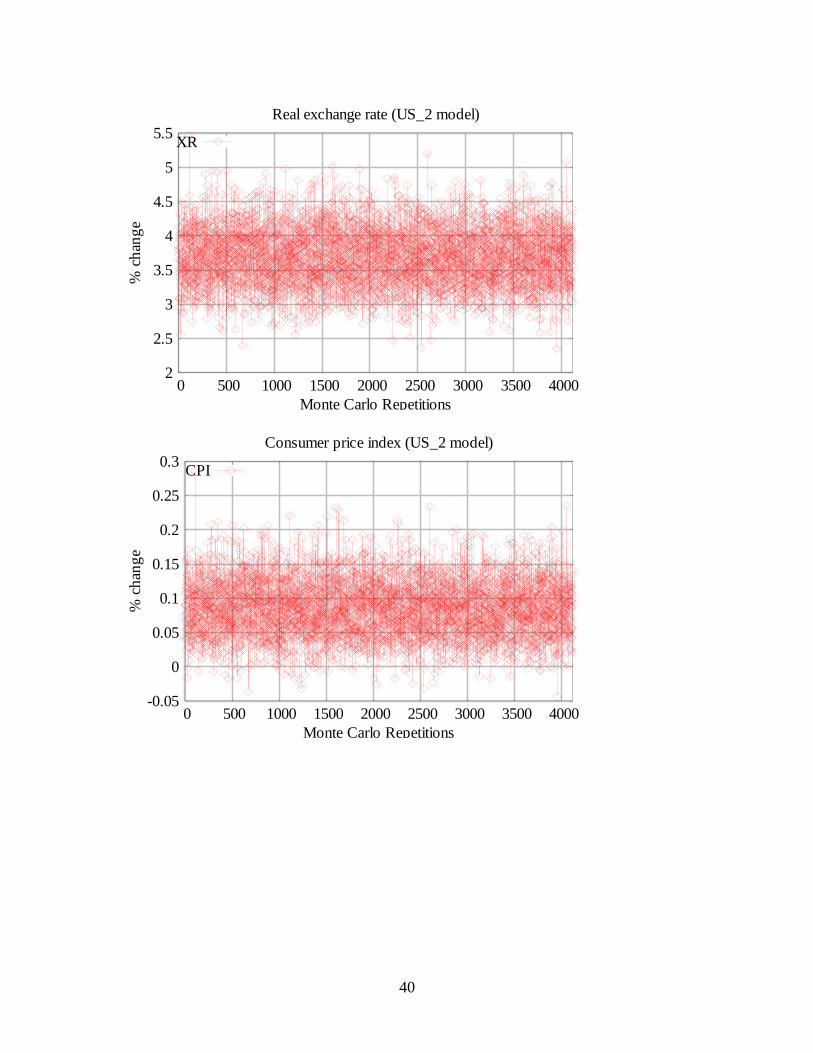
6.3 Variation in model variables under different exogenous parameter
assumptions
6.3.1 U.S. model variables – Scenario 2
Note: 82.6% of the models have been successfully solved, e.g. around 4,100 outcomes of
the each result variable are available.
Source for all figures: Own calculations.
100000
110000
120000
130000
140000
150000
160000
170000
180000
0 500 1000 1500 2000 2500 3000 3500 4000
Abs
olut
e ch
ange
(Mill
ion
Dol
lar)
Monte Carlo Repetitions
Value added (US_2 model)
GDP
1.4e+006
1.6e+006
1.8e+006
2e+006
2.2e+006
2.4e+006
2.6e+006
0 500 1000 1500 2000 2500 3000 3500 4000
Abs
olut
e ch
ange
(wor
kers
)
Monte Carlo Repetitions
Total employment (US_2 model)
QFS
39
2
2.5
3
3.5
4
4.5
5
5.5
0 500 1000 1500 2000 2500 3000 3500 4000
% c
hang
e
Monte Carlo Repetitions
Real exchange rate (US_2 model)
XR
-0.05
0
0.05
0.1
0.15
0.2
0.25
0.3
0 500 1000 1500 2000 2500 3000 3500 4000
% c
hang
e
Monte Carlo Repetitions
Consumer price index (US_2 model)
CPI
40
0.9
1
1.1
1.2
1.3
1.4
1.5
1.6
0 500 1000 1500 2000 2500 3000 3500 4000
% c
hang
e
Monte Carlo Repetitions
Factor return: Capital (US_2 model)
FR
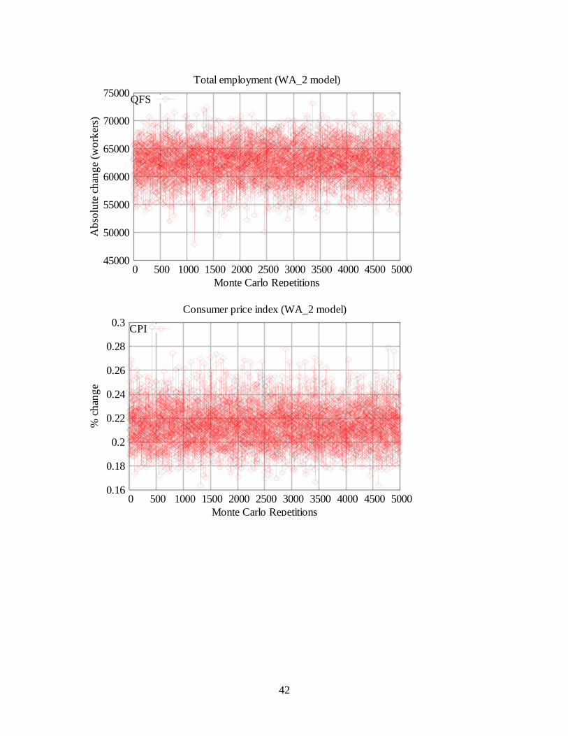
6.3.2 Washington State model variables – Scenario 2
Note: 96.8% of the models have been successfully solved, e.g. around 4,900 outcomes of