Improved Added Mass and Wet Modes Calculation for Naval...

Defence R&D Canada

Improved Added Mass and Wet Modes

Calculation for Naval Structures

M.J. Smith

Technical Memorandum

DRDC Atlantic TM 2003-084

May 2003

Copy No.________

Defence Research andDevelopment Canada

Recherche et développementpour la défense Canada

Improved Added Mass and Wet ModesCalculation for Naval Structures

M. J. Smith

Defence R&D Canada – Atlantic

Technical Memorandum

DRDC Atlantic TM 2003-084

May 2003

Abstract

Several improvements have been made to the added mass and wet mode calculation mod-ules in DRDC’s VAST finite element program. The performance of the improved softwareis described on the basis of accuracy and computational efficiency. For finite element mod-els with approximately two thousand boundary elements on the wetted surface of the struc-ture, the performance of the added mass computation module is improved by a factor ofthirty. In larger problems the performance gain is even greater. Moreover, it is shown thatthese improvements are achieved without any loss of accuracy.

Methods for predicting the natural vibration modes of floating or submerged naval struc-tures are also reviewed. The dry mode approximation method is shown to be capable ofcalculating the low frequency wet modes with good accuracy and much better performancethan a direct eigensolution of the wetted structure. The performance of the dry mode ap-proximation has also been improved for large models. Finally, the VAST sparse solver isimplemented for use in the direct eigensolution and dynamic response of wetted structures.The performance achieved with the sparse solver is shown to be significantly better thanthat obtained with VAST’s profile solver.

Resume

Nous avons apporte plusieurs ameliorations aux modules de calcul de masse ajoutee et decalcul en mode humide dans le logiciel VAST, le programme de calculs par elements finisde RDDC. Nous presentons les ameliorations apportees au logiciel, notamment au chapitrede la precision et de l’efficacite des calculs. Les calculs du module de la masse ajouteepour un modele d’elements finis comportant pres de deux mille elements de frontiere surla surface immergee d’une structure sont trente fois plus rapide que ceux de la versionanterieure. Pour les grands problemes, l’amelioration du rendement est encore plus grande.De plus, nous demontrons que ces ameliorations ne sont pas accompagnees par une pertede precision.

Nous examinons egalement les methodes de predictions des modes de vibration naturelle destructures navales flottantes ou immergees. Nous montrons que la methode d’approximationen � mode sec � permet de calculer les modes humides a basse frequence avec une bonneprecision et plus rapidement qu’une solution propre directe de la structure immergee. Lerendement de l’approximation du mode sec est egalement meilleur pour les grands modeles.Finalement, nous utilisons le solutionneur de matrice creuse pour calculer la solution propredirecte et la reponse dynamique des structures immergees. Nous montrons que le rendementdu solutionneur de matrice creuse est tres superieur a celui du factorisateur par methode deprofil.

DRDC Atlantic TM 2003-084 i

This page intentionally left blank.

ii DRDC Atlantic TM 2003-084

Executive summary

Background

When predicting the vibration or dynamic response of a floating or submerged naval struc-ture, the influence of the surrounding water has to be accounted for. This is called the fluidadded mass effect. DRDC’s VAST finite element program can be used to predict the fluidadded mass and its influence on a structure’s behaviour. But recent work to determine theslamming response of the KINGSTON class structure has revealed a number of limitationsin VAST for this type of analysis. The present work describes the improvements that havebeen made to the VAST code and documents the resulting performance gains.

Principal Results

For models with about 2000 fluid panel elements, the VAST module for calculating fluidadded mass runs about thirty times faster than it did before. In larger problems, the perfor-mance gains are even greater. Several test problems illustrate the high level of performancethat can now be achieved. Two methods for calculating the vibration behaviour of a floatingor submerged structure are presented. In one, the vibration modes of the wet structure areapproximated from those of the dry structure. In the other method, the modes of the wetstructure are calculated directly. It is shown that the approximate method is much moreefficient and generally provides acceptable accuracy.

Significance of Results

As a result of the improvements described in this study, the slamming analysis of theKINGSTON class was able to proceed in a timely manner. Added mass and wet modecalculation of this naval hull structure, which was previously beyond the capability of thesoftware, can now be done in about an hour using a standard desktop computer.

As the HALIFAX class approaches midlife and design changes are being considered as partof a future refit, rapid evaluations of the vibration modes and other response characteristicsof the structure will be necessary. It is shown in this study that the primary hull girdervibration modes of the HALIFAX class structure, including added mass effects, can nowbe calculated in just a few minutes.

M. J. Smith; 2003; Improved Added Mass and Wet Modes

Calculation for Naval Structures; DRDC Atlantic TM 2003-084;

Defence R&D Canada – Atlantic.

DRDC Atlantic TM 2003-084 iii

Sommaire

Contexte

Il est necessaire de tenir compte de l’influence de l’eau, lorsque l’on predit les vibrations oula reponse dynamique d’une structure navale flottante ou immergee. On parle de l’effet dela masse ajoutee par le fluide. On peut predire la masse ajoutee par le fluide et son influencesur le comportement d’une structure a l’aide du logiciel VAST, le programme de calculs parelements finis de RDDC. Or, des travaux recents pour etudier la reponse de la structure desnavires de la classe Kingston au tossage ont permis de deceler certaines limites du logicielpour ce type d’analyse. Le present rapport presente les ameliorations effectuees au logicielVAST et ses documents connexes, ainsi que les gains de rendement obtenus.

Resultats principaux

Lors du calcul de modeles comportant 2000 elements de panneaux immerges, la nouvelleversion du module VAST de calcul de la masse ajoutee s’est averee trente fois plus rapideque la version anterieure. Pour les problemes plus grands, le gain est encore superieur. Plu-sieurs problemes tests illustrent le haut rendement actuellement atteint par le programme.Nous presentons deux methodes de calcul du comportement vibratoire des structures flot-tantes ou immergees. Dans la premiere, on approxime les modes de vibration de la structureimmergee a partir de ceux de la structure seche. La seconde calcule directement les modesde la structure immergee. Nous montrons que la methode par approximation est beaucoupplus efficace et qu’en general, elle est suffisamment precise.

Importance des resultats

A la suite des ameliorations decrites dans ce rapport, on a pu proceder rapidement a l’ana-lyse du tossage des navires de la classe Kingston. Il est maintenant possible de realiser surun ordinateur de bureau ordinaire, en une heure environ, des calculs de masse ajoutee etdans le mode humide qui etaient impossibles avec la version anterieure du logiciel.

La moitie de la vie utile des navires de la classe Halifax sera bientot ecoulee et, dans le cadred’une refonte a venir, l’on etudie les changements de conception. Ainsi, il sera necessairede pouvoir evaluer rapidement les modes de vibration et d’autres caracteristiques de lareponse de la structure. Cette recherche nous a permis de montrer que seulement quelquesminutes sont necessaires au calcul des modes de vibration de la poutre-coque principale desstructures de la classe Halifax, incluant les effets de masse ajoutee.

M. J. Smith; 2003; Ameliorations apportees aux modules de calcul de

la masse ajoutee et de calcul en mode humide pour les structures

navales; DRDC Atlantic TM 2003-084; RDDC Atlantique.

iv DRDC Atlantic TM 2003-084

Table of contents

Abstract . . . . . . . . . . . . . . . . . . . . . . . . . . . . . . . . . . . . . i

Resume . . . . . . . . . . . . . . . . . . . . . . . . . . . . . . . . . . . . . i

Executive summary . . . . . . . . . . . . . . . . . . . . . . . . . . . . . . . iii

Sommaire . . . . . . . . . . . . . . . . . . . . . . . . . . . . . . . . . . . . iv

Table of contents . . . . . . . . . . . . . . . . . . . . . . . . . . . . . . . . v

List of figures . . . . . . . . . . . . . . . . . . . . . . . . . . . . . . . . . . vi

List of tables . . . . . . . . . . . . . . . . . . . . . . . . . . . . . . . . . . . vi

1 Introduction . . . . . . . . . . . . . . . . . . . . . . . . . . . . . . . 1

2 Improvements to the Fluid Added Mass Calculation . . . . . . . . . . 1

2.1 Inversion Algorithm . . . . . . . . . . . . . . . . . . . . . . . 4

2.2 Storage Files . . . . . . . . . . . . . . . . . . . . . . . . . . 5

2.3 Transformation to Finite Element Coordinates . . . . . . . . . 6

2.4 Generalization of Reflection Planes . . . . . . . . . . . . . . . 7

3 Vibration Modes of Marine Structures . . . . . . . . . . . . . . . . . 9

3.1 Review of Wet Mode Calculation Methods . . . . . . . . . . . 9

3.1.1 Direct Method . . . . . . . . . . . . . . . . . . . . . . 9

3.1.2 Dry Mode Approximation . . . . . . . . . . . . . . . 10

3.2 Improvements to the Wet Mode Calculation . . . . . . . . . . 10

3.2.1 Direct Analysis with the Sparse Solver . . . . . . . . . 10

3.2.2 Improved Efficiency in Dry Mode Approximation . . . 11

4 Sample Test Problems . . . . . . . . . . . . . . . . . . . . . . . . . . 12

4.1 Cylinder Models . . . . . . . . . . . . . . . . . . . . . . . . 12

4.2 Stiffened Panel Model . . . . . . . . . . . . . . . . . . . . . . 16

DRDC Atlantic TM 2003-084 v

4.3 HALIFAX Class Global Model . . . . . . . . . . . . . . . . . 17

4.4 KINGSTON Class STC Hull Structure . . . . . . . . . . . . . 20

5 Conclusion . . . . . . . . . . . . . . . . . . . . . . . . . . . . . . . 20

References . . . . . . . . . . . . . . . . . . . . . . . . . . . . . . . . . . . . 22

Annex . . . . . . . . . . . . . . . . . . . . . . . . . . . . . . . . . . . . . . 23

A List of symbols, abbreviations, acronyms and initialisms . . . . . . . 23

List of figures

1 KINGSTON class hull structure in way of sewage treatmentcompartment (STC) . . . . . . . . . . . . . . . . . . . . . . . . . . . 2

2 Organization of VAST’s Added Mass Module ADMAS5. . . . . . . . 3

3 Image Sources Produced by Reflections in a Symmetry Plane and aFree Surface. . . . . . . . . . . . . . . . . . . . . . . . . . . . . . . 8

4 Cylinder model showing the wet surface (magenta) in the floatingcondition. . . . . . . . . . . . . . . . . . . . . . . . . . . . . . . . . 14

5 KINGSTON class stiffened panel model . . . . . . . . . . . . . . . . 17

6 HALIFAX class global model . . . . . . . . . . . . . . . . . . . . . 18

List of tables

1 Models for testing fluid mass . . . . . . . . . . . . . . . . . . . . . . 13

2 Added mass results for a submerged cylinder . . . . . . . . . . . . . 13

3 Execution times in seconds for added mass and modal calculations . . 14

4 Added mass results for a floating cylinder . . . . . . . . . . . . . . . 15

5 Execution times in seconds for factorization . . . . . . . . . . . . . . 15

6 Execution times in seconds for eigenvalue solutions . . . . . . . . . . 15

vi DRDC Atlantic TM 2003-084

7 Wet natural frequencies (Hz) for the cylinder models . . . . . . . . . 16

8 Wet natural frequencies (Hz) for the stiffened panel model . . . . . . 18

9 Wet modes (Hz) for the HALIFAX global model . . . . . . . . . . . . 19

10 Hull girder mode shape notation (� denotes an integer value) . . . . . 19

11 Wet natural frequencies (Hz) for the STC detail model. . . . . . . . . 21

DRDC Atlantic TM 2003-084 vii


viii DRDC Atlantic TM 2003-084

1 Introduction

Natural frequency and dynamic analyses of marine structures require the inclusionof the inertia of water entrained by the motion of the structure. This is knownas the fluid added mass effect. In finite element analysis, the use of fluid addedmass became standard practice in the 1980s, and methods for calculating the fluidmass were implemented in DRDC’s VAST [1] finite element code at that time. Ithas long been noted that structural analysis with VAST using fluid added mass wasexcessively time consuming, whether it was through using the fluid volume elementor boundary element (panel) method. In the case of the panel method, models withmore than four thousand panels were generally impractical to analyse because ofthe excessive cost of calculating the fluid added mass matrix.

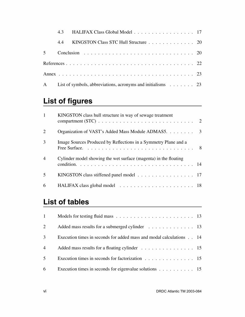
Recently, a slamming analysis was performed on the KINGSTON class structureduring the course of which a number of deficiencies in VAST came to light in re-lation to its handling of fluid added mass and its effects. In particular, with a hullstructure model with more than five thousand panels (Figure 1), the fluid addedmass calculation executed for more than twenty-four hours without nearing com-pletion. By contrast, the eigenvalue analysis of the dry structure could be performedin just a few minutes using the new sparse solver in VAST [2]. Given this widediscrepancy in performance, it was apparent that the VAST fluid mass calculationmodule ADMAS5 had serious problems that required addressing. This report de-scribes and demonstrates the improvements made.

2 Improvements to the Fluid Added MassCalculation

Fluid added mass can be calculated using either the fluid volume element methodor the boundary element (panel) method. Vernon [3] showed that the panel methodwas much more efficient than the fluid volume element method. The principaladvantages of the panel method are as follows:

1. Only the wet surface of the structure is modelled;

2. An unbounded fluid domain is systematically accounted for;

3. Including the fluid added mass in the structural model does not increase thenumber of degrees of freedom.

The main drawback of the panel method is that the fluid added mass is nonsymmet-ric and fully coupled.

DRDC Atlantic TM 2003-084 1

Figure 1: KINGSTON class hull structure in way of sewage treatment compartment(STC)

The boundary element fluid mass calculation currently in VAST was originally de-veloped at DREA in the late 1980s as a standalone program called ADMASS. Laterit was incorporated into the VAST program as the module ADMAS5. Theoreticaldescription and implementation details are given in Reference [3], and will not berepeated here except where necessary. Two boundary element formulations wereprovided: a “source” formulation and a “dipole” formulation. The user can also in-clude a free surface if the structure is floating, and a symmetry plane can be definedfor half-models of symmetric structures.

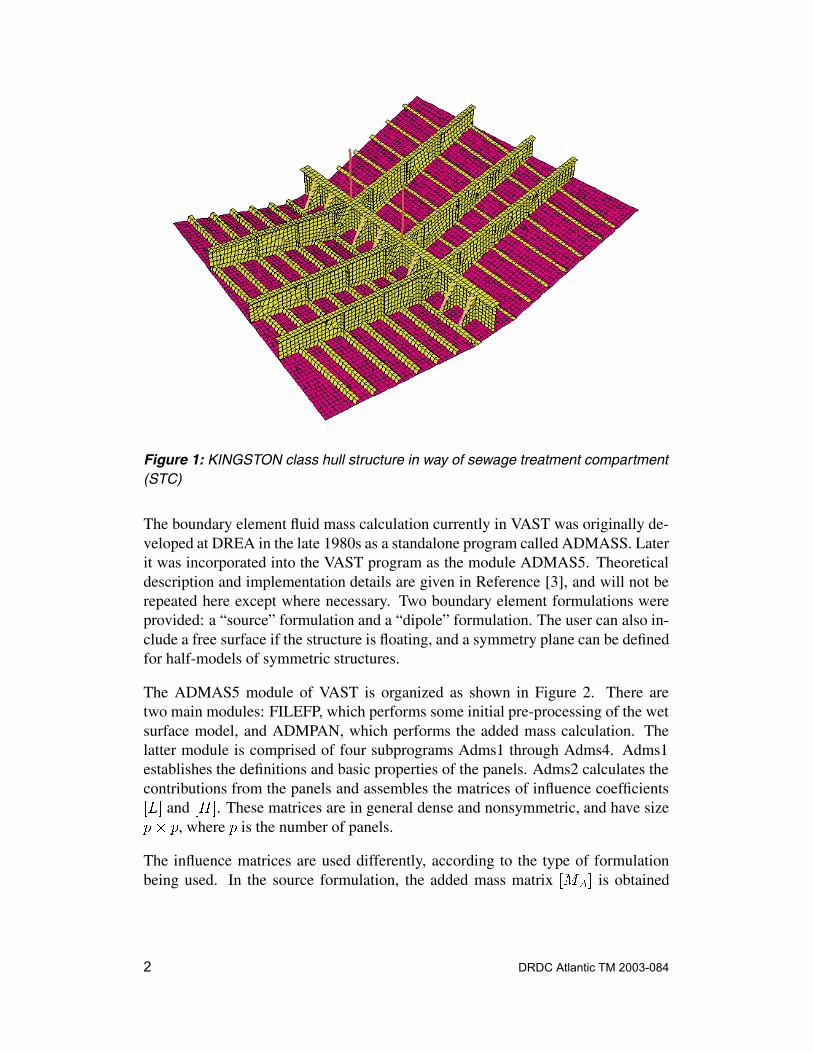
The ADMAS5 module of VAST is organized as shown in Figure 2. There aretwo main modules: FILEFP, which performs some initial pre-processing of the wetsurface model, and ADMPAN, which performs the added mass calculation. Thelatter module is comprised of four subprograms Adms1 through Adms4. Adms1establishes the definitions and basic properties of the panels. Adms2 calculates thecontributions from the panels and assembles the matrices of influence coefficients�� and ��. These matrices are in general dense and nonsymmetric, and have size�� , where � is the number of panels.

The influence matrices are used differently, according to the type of formulationbeing used. In the source formulation, the added mass matrix �� is obtained

2 DRDC Atlantic TM 2003-084

FILEFPPre-processing

ADMPANAdded mass calculation

Adms1Panel definitions

Adms2Influence coeffs [L], [H]

Adms3Inversion of [L]

Adms4Calculate & store [MA]

Figure 2: Organization of VAST’s Added Mass Module ADMAS5.


through the following matrix product

�� (1)

whereas the dipole formulation uses:

�� (2)

Here, �� is a diagonal matrix of the panel surface areas, and �� is a coordinatetransformation matrix between the finite element nodal coordinates and the panelnormal coordinates. The �� obtained from these formula is square and not sym-metric. Since symmetric mass matrices are usually required for structural analysis,the calculated �� can be explicitly made symmetric by averaging off-diagonalpairs. This is not believed to greatly detract from the accuracy [3].

In the original version of ADMAS5, the Adms3 subprogram calculated �� from�� using an iterative (Gauss-Seidel) inversion algorithm and stored the inverse ina scratch file. Adms4 then performed the matrix products in the above formulas,using the stored ��. This approach to the numerical computation of �� isseriously flawed for reasons that are explained in the following subsections.

2.1 Inversion Algorithm

The calculation of �� or �� is computationally the most expensive stepin the formation of the added mass matrix. This step must be performed efficientlyif good performance is to be achieved. Explicitly inverting �� and then pre- or post-multiplying the inverse with �� is a poor way to compute these products. A muchbetter way is to calculate the matrix products directly by solving a linear system ofequations. For example, with the dipole formulation solving,

�� (3)

and for the source formulation solving,

�� (4)

gives the desired results � � �� and � � ��, respectively.

Efficient solution of (3) and (4) involves LU factorization of �� (or �� ) followedby backward and forward solutions of the factorized equations. LU factorization of�� requires �� floating point operations (flops), while the forward and backwardsolution of each right-hand side requires � and � flops respectively [4]. Thus thetotal flops needed to obtain the solutions is �� . Bycontrast, the iterative solution using Gauss-Seidel requires �� flops per iteration,


per right-hand side vector [4]. Assuming an average of three iterations per solutionvector, a complete inversion of �� would require �� flops. Add to thatthe �� flops needed for the subsequent matrix-matrix product and the total effort is��. Using the factorization approach therefore saves �� flops. In addition, thesmaller number of operations reduces the risk of round-off error occuring, whichcan be a serious concern when manipulating large matrices in single precision.

The implementation of the new approach in Adms3 was accomplished by usingLAPACK [5] subroutines SGETRF and SGETRS for the LU factorization and so-lution steps, respectively. LAPACK is public domain software for numerical linearalgebra applications which was developed through the collaborative efforts of sev-eral government and university institutions in the United States. The software isavailable through www.netlib.org.

The function of Adms3 has changed by virtue of this modification to the algorithm.Originally, Adms3 provided only ��, while in the new form, it provides one ofthe two product forms �� or ��, according to the formulation beingused. This reduces the work that needs to be subsequently performed in Adms4.

With the LAPACK routines now implemented, the LU factorization and solutionsteps are performed in core, and no auxiliary storage is required. Two �� singleprecision matrices are used for these operations. One holds the original �� (or �� )matrix and is overwritten with the LU factorization as it is being calculated. Theother holds the original �� (or �� ) matrix, and is used to hold the solution vectors� (or � ) as they are calculated. The solution vectors are then passed directly toAdms4 without temporary storage and retrieval.

In the original version of Adms3, one � � � single precision matrix was used plussome additional working arrays. But because of an implementation error, the �� matrix was dynamically allocated in double precision, and was therefore using theequivalent of two �� single-precision matrices. Since the new version of Adms3requires two � � � single-precision matrices, the memory used by the new versionis about the same as in the old version.

2.2 Storage Files

The original ADMASS program was designed to run on the computers of the dayand thus relied heavily on auxiliary storage to pass data from one subprogram toanother. An example of this was the storage of �� in Adms3 and its retrieval inAdms4. Scratch files were also used to temporarily store data within subroutines,for example during matrix-matrix product calculations.

As a result of the changes made to Adms3 described in the previous section, the


matrix �� is not explicitly formed, and therefore the INVERS.MAS file used tostore this matrix is no longer needed.

In the original version of Adms4, the �� matrix was retrieved row-by-row fromINVERS.MAS and either pre- or post-multiplied by the influence matrix ��, de-pending on which formulation is being used. The product of these two matriceswas then stored row-by-row on a scratch file PREFX.RAN. By directly passing thesolution vectors to Adms4, this storage and retrieval to and from PREFX.RAN isavoided.

The total savings in I/O achieved through these changes is ��.

2.3 Transformation to Finite Element Coordinates

Once the matrix product �� or �� has been formed, the next step is topremultply by ��, the diagonal matrix of panel areas. This is a relatively trivial stepand is performed with small cost. This operation produces a nonsymmetric fluidadded mass matrix in panel coordinates, and will be denoted as ��, to distinguishit from the nodal fluid added mass matrix ��. At this point symmetry can beenforced on ��.

The final step is to apply the matrix �� to transform the matrix from panel coordi-nates to finite element nodal coordinates. The matrix �� has size �� , where �is the number of nodes on the wetted surface. It is also a highly sparse matrix andcan be stored in a compact form. For example, if the wetted surface is meshed with4-node boundary elements the �� matrix can be condensed to size �� .

In the original version of Adms4, a fairly laborious process was used to perform thepre-multiplication by �� and post-multiplication by �� . The steps taken were asfollows.

1. The ��matrix �� was held in memory, and the columns of �� were formedin succession and post-multiplied with ��.

2. The resulting �� matrix �� was stored in a scratch file.

3. Each each row of �� was then formed and premultiplied by the entire matrix�� , which had to be read column-by-column from its scratch file.

4. The resulting columns of �� are permanently stored on the file PREFX.T36

As �� has �� rows, �� had to be retrieved a total of �� times in Step 3. Thetotal number of I/O operations for the above four-step process is �� .


For models where � is large and � � �, the above I/O requirements are so excessivethat the added mass calculation is all but impossible. For example, with � � � ��, over 2000 GB of I/O is needed in Adms4. Note that finite element modelswith four thousand panels on the wetted surface are by no means unusual by today’sstandards.

To correct this problem, the code was modified so that �� is assembled in com-pact form and held in memory during the pre- and post-multiplications. The orderof loops in the pre-multiplication could then be reversed so that each column of�� can premultiplied by the whole of �� directly. The pre-multiplication op-eration can thus be performed with a single retrieval of �� from scratch. This,combined with the original storage of �� on scratch and the permanent storageof ��, makes the total I/O requirement for Adms4 equal to �� , which issmaller than the original requirement by a factor of about ��. For example, in amodel with � � ��, the total I/O now needed is now about 900 MB.

The cost of this improvement is that �� now has to be held in memory. But it wasfound that the memory used to store the LU factorization of �� in Adms3 could bere-used for storing �� in Adms4. Since �� is generally smaller than ��, the totalmemory requirement for Adms4 is not increased over what is required for Adms3.

2.4 Generalization of Reflection Planes

The original version of ADMASS allowed the user to define two types of reflectionplane: a free surface and a symmetry plane. The program provided options forinvoking one, or the other, or both of these reflection planes together. A free surface,if defined, had to be in the global XY plane; a symmetry plane had to be in theglobal XZ plane. These restrictions are too limiting for practical use, as it mayoften be convenient to orient a model of a surface ship with the Y axis, not theZ, for example, as the vertical. Furthermore, it may be convenient to offset a freesurface or symmetry plane from one of the global coordinate planes.

The latter problem is easier to address than the former. A wetted surface modelcan be translated in any direction without affecting the resulting fluid added massmatrix. The pre-processing module FILEFP already allows for this type of trans-lation to position a free surface on the global XY plane. It is a simple matter togeneralize this feature to allow translation of the model along any of the coordinateaxes so as to position either a free surface or a symmetry plane on the desired globalcoordinate planes.

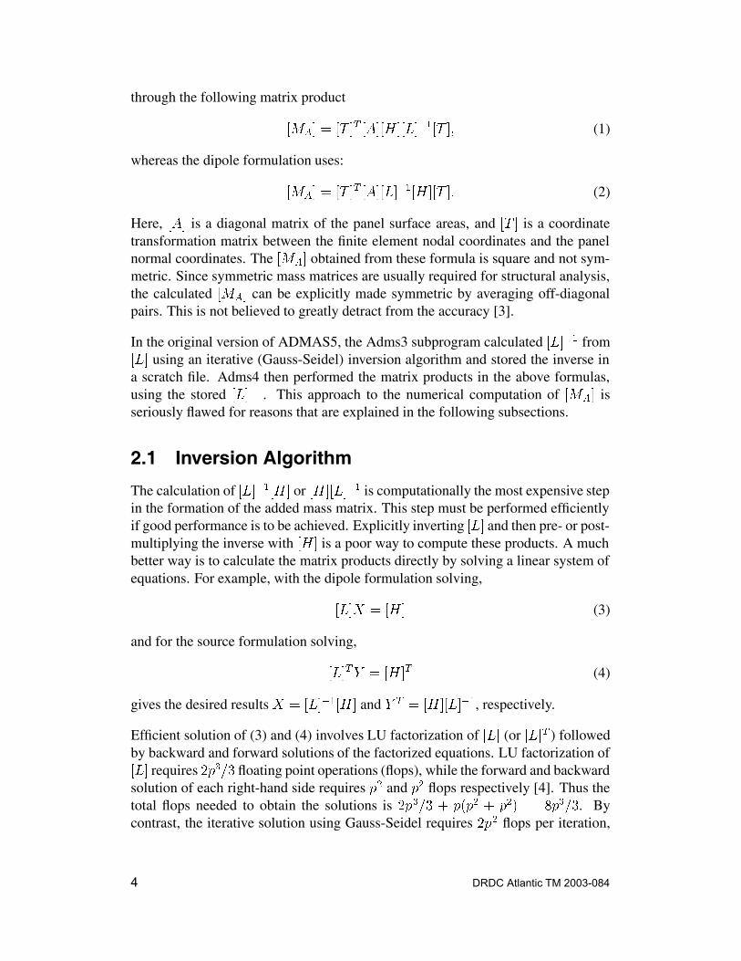
To allow different orientations of the reflection planes, one possible solution is tosimply rotate the wetted surface model until a reflection plane is parallel to the


Image -Q

Image +QSource +Q

Free surface

Symmetry plane

+ +

++Image -Q

Wet surface

Figure 3: Image Sources Produced by Reflections in a Symmetry Plane and aFree Surface.

desired global coordinate plane. But such a rotation changes the values in the re-sulting fluid added mass matrix, requiring a subsequent counter-rotation of the fluidmass terms to obtain a matrix that is compatible with the original model. This isan impractical way of approaching the problem. Instead, it was decided to directlygeneralize the reflection plane definitions where they are implemented in the codeso that any of the global planes can be used as either a free surface or a symmetryplane.

Reflection planes are used in the boundary element calculation of the influencecoefficients that make up �� and ��. Details about the computation of these termsare given in Reference [3]. Each of these terms represent the influence of one panelon another, where one panel acts as a “source” and the other panel as a “receiver”.The Green’s function between the two determines the strength of the influence.When a reflection plane is present, imaging of the source point occurs. Figure 3shows the imaging of a source point of strength� in a free surface and a symmetryplane. For reflections in a free surface a negative image can be used to create azero-pressure condition at the plane of the surface.

Generalization of the reflection planes was achieved by altering the code to allowfor more generalized positioning of the image sources. It was found that this couldbe done without a great amount of modification of the existing code. Subsequenttesting of models with free surface or symmetry planes showed that the resultingnet added mass was the same for different orientations of the model.

It should be noted that the definitions of the waterplane and symmetry planes arestill somewhat restrictive in that they still must be parallel to one of the coordinate


planes. But this should not be a very great restriction as ship models are usuallyoriented so that their principal axes are aligned with the coordinate axes. Moreover,it is convenient to orient marine structures with symmetry so that their planes ofsymmetry are parallel to the coordinate planes.

3 Vibration Modes of Marine Structures

3.1 Review of Wet Mode Calculation Methods

In the past, various methods for calculating the modes of submerged or floatingstructures have been studied numerically and experimentally [6, 7]. Based on thiswork, two methods for calculating the undamped natural vibration modes of wettedstructures were implemented in VAST. These are reviewed in the following.

3.1.1 Direct Method

In this method the fluid added mass matrix is assembled directly into the governingalgebraic eigenvalue equation as follows:

�� (5)

where �� and �� are the stiffness and mass matrices of the structure. Note thatthe fluid added mass �� is only nonzero at translational degrees of freedom onthe wetted surface of the structure. The matrix �� is needed to transform �� soas to make it compatible with the assembled structural matrices.

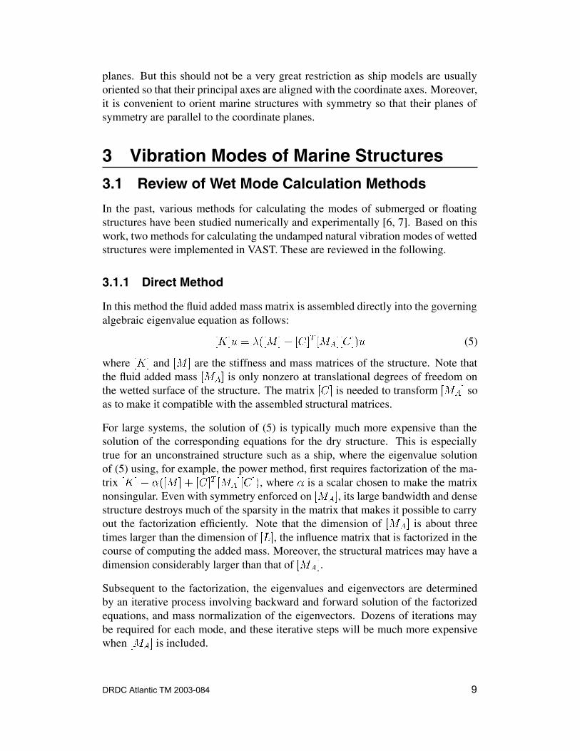
For large systems, the solution of (5) is typically much more expensive than thesolution of the corresponding equations for the dry structure. This is especiallytrue for an unconstrained structure such as a ship, where the eigenvalue solutionof (5) using, for example, the power method, first requires factorization of the ma-trix �� , where � is a scalar chosen to make the matrixnonsingular. Even with symmetry enforced on ��, its large bandwidth and densestructure destroys much of the sparsity in the matrix that makes it possible to carryout the factorization efficiently. Note that the dimension of �� is about threetimes larger than the dimension of ��, the influence matrix that is factorized in thecourse of computing the added mass. Moreover, the structural matrices may have adimension considerably larger than that of ��.

Subsequent to the factorization, the eigenvalues and eigenvectors are determinedby an iterative process involving backward and forward solution of the factorizedequations, and mass normalization of the eigenvectors. Dozens of iterations maybe required for each mode, and these iterative steps will be much more expensivewhen �� is included.


3.1.2 Dry Mode Approximation

An alternative approach is to use a dry mode approximation for the wet modes ofthe structure. Denote �� as a matrix whose columns are eigenvectors for the drystructure calculated from the equation

�� (6)

Let � be the number of dry modes included in ��, where � is typically muchsmaller than � , the total number of degrees of freedom in the structure. The equa-tion

� � �� (7)

represents a transformation from modal coordinates � to physical coordinates �. Inpractical terms it signifies that the range of values for � is limited to those that canbe expressed as a linear combination of the columns of ��.

Applying (7) to (5), and premultiplying by �� gives the following symmetric

system of equations:

��

� �� (8)

It can be assumed without loss of generality that the dry modes are normalized suchthat �� and ��

� �� , where �� is the identity matrixand �� is a diagonal matrix containing the eigenvalues of the dry structure. Thefollowing simplified eigenvalue equation is then obtained

�� (9)

This system of equations is the approximate, or reduced, eigenvalue problem for thewetted structure. The coefficient matrices have dimension�� and can thereforebe solved at small cost. The eigenvalue, eigenvector pairs �� define the wetmodes of the structure. The wet eigenvectors can be reconstructed in physical spaceusing (7).

3.2 Improvements to the Wet Mode Calculation3.2.1 Direct Analysis with the Sparse Solver

A sparse equation solver was previously developed at DRDC and implemented inVAST for static, dynamic, and eigenvalue analysis of dry structures [2]. The perfor-mance obtained with the sparse solver was extremely good, and so it was decidedto extend its implementation to modal and dynamic analysis of wetted structures.

It was determined that the best way to include the fluid mass in the sparse solveris to treat the entire fluid added mass matrix as a special element type with a fullcoupled element mass and zero stiffness. This approach required two main tasks:


1. Inclusion of the connectivity array for the fluid added mass in the node orderingalgorithm.

2. Assembly of the fluid added mass into the global effective stiffness matrix (forunrestrained or partially restrained structures) and the global mass matrix.

It is expected that the fully coupled nature of the fluid mass will effectively destroymuch of the sparsity in the global matrices, thereby depriving the sparse solverof its primary advantage. Nonetheless, it was hoped that the sparse solver wouldstill provide better performance than the existing profile solver due to its betterhandling of memory and I/O. The implementation was successfully completed andthe performance of the sparse solver with fluid added mass is given for various testproblems in Section 4 (see Tables 5 and 6).

3.2.2 Improved Efficiency in Dry Mode Approximation

Calculation of wet modes using the dry mode approximation is implemented in theVAST module EIGNWM, and is made up of three major tasks:

1. Formation of the reduced equation (9);

2. Solution of the eigenvalues and eigenvectors of (9);

3. Reconstruction and normalization of the wetted eigenvectors in physical space.

Inspection of the algorithms in EIGNWM immediately revealed some areas whereimprovement was possible. In the forming the equation (9), the most costly opera-tion is computing the matrix product �� . In performing this ma-trix product, �� is never explicitly formed but is rather invoked implicitly throughinteger connectivity arrays.

The EIGNWM module is arranged so that the matrix product is performed intwo steps: the formation of the � � � array �� , followed by pre-multiplication by ��

� . In the existing version of the code, the first step is per-formed for each mode in turn, so that �� has to be read from disk a total of� times. The computed vectors (dimension � � �) are written to a scratch file.In the premultiplication step, these vectors were retrieved from scratch and pre-multiplied by each dry mode in turn, this required a total of � retrievals of eachvector. In addition to this, the dry modes themselves were stored on a random ac-cess scratch file and were retrieved once in the post-multiplication, and once in thepre-multiplication steps. Thus the total amount of data stored or retrieved duringStep 1 was�� .

The goal of the changes made in this study was to reduce the amount of I/O in theStep 1 calculation at the cost of increased memory usage. This was thought to be a


worthwhile trade-off, given that the existing EIGNWM under-utilized the availablememory. The approach was to allocate two arrays of size��, one to hold the drymodes ��, and the other to hold the product vectors �� . The innerproduct calculation can then be done with a single retrieval of �� from disk. Noother I/O is required to complete Step 1, and so the total I/O is now ��, a reductionof more than a factor of �. The cost is an increase in memory usage by ��.

A second area where improvement was achieved is in Step 3. The normalization ofthe wet modes was formerly performed in physical space by calculating the gener-alized masses

� � �� (10)

where �� denotes a wet mode in physical coordinates. The �� are then scaled sothat the generalized mass will be one. This inner product was performed for eachmode in turn, so that a total of � retrievals of �� from disk were required.

Substituting the dry mode approximation �� into the generalized massexpression gives,

� � ��

� �� (11)

The term in parenthesis on the right is identical to the reduced-order mass matrixin (9). Thus the generalized masses in physical and modal space are the same,and normalizing the eigenvectors � is equivalent to normalizing ��. The reduced-order mass matrix has already been calculated in Step 1, and is small enough tobe held in core. The normalization of � can therefore be performed at little cost,and this avoids the greater expense of computing the inner products in (10). It alsoeliminates a further� retrievals of �� from disk, and eliminates the need to storethe dry modes on a random-access scratch file. An additional simplification is thatthe structural mass �� is no longer needed in the wet mode calculation: only thedry modes ��, �� and the fluid mass �� are required.

4 Sample Test Problems

The accuracy and efficiency of the modified version of ADMAS5 has been testedon several models ranging in size from 630 to 10,818 nodes. A summary of the testmodels is given in Table 1. Detailed description of the testing performed is given inthe following sections.

4.1 Cylinder Models

Theoretical values for fluid added mass are available for infinitely long rigid cylin-ders. For a fully submerged cylinder in lateral motion, the added mass per unit


Table 1: Models for testing fluid mass

Model Structural Nodes Fluid Panels Total DOFFloating Cylinder 630 300 3780Submerged Cylinder 630 600 3780Stiffened panel 2362 1658 14,172HALIFAX global 7853 1976 47,118STC detail 10,818 5566 64,908

Table 2: Added mass results for a submerged cylinder

ADMAS5 Added Mass (tonnes)Version Source DipoleExisting 29.04 29.04Modified 29.03 29.03

length is ��, where � is the density of water, and � is the cylinder radius. Fora floating cylinder in which half of the volume is submerged, the theoretical addedmass per unit length is �� in heave and �� in sway.

The cylinder model in Figure 4 was tested in both fully submerged and floatingconditions. The model has a radius of one metre, a length of ten metres, and ismeshed with 600 4-node shell elements. The ends of the cylinder are neglected. Thefully submerged cylinder has 600 4-node boundary elements on the wet surface,whereas the floating cylinder has just 300 elements on the wet surface.

The total added mass computed for the submerged cylinder is given in Table 2 forboth the existing and modified versions of ADMAS5, and for the source and dipoleformulations. The theoretical value for this cylinder is 31.4 tonnes. The differenceof less than ten percent between the theoretical and ADMAS5 results is due to theassumption of an infinite length in the theoretical result. There is no appreciabledifference between the source and dipole formulations in this example. Table 3gives the execution times for the two versions ADMAS5, demonstrating the muchimproved performance of the modified version even for this relatively small model.The execution times were obtained on a desktop PC with a Pentium 4, 1.8 GHzprocessor, and 1 GB of RAM. The timings for the source and dipole formulationsare nearly the same, and so only one set of times is reported.

The results computed for the floating cylinder are given in Table 4. A reflectingplane with a pressure-release condition was included to represent the free surfacein these calculations. The theoretical values for this case are 15.7 tonnes in heave


Figure 4: Cylinder model showing the wet surface (magenta) in the floatingcondition.

Table 3: Execution times in seconds for added mass and modal calculations

Model Existing ModifiedFloating Cylinder

ADMAS5 11.64 2.89EIGEN1 (20 modes) 6.50 5.02

Submerged CylinderADMAS5 65.75 8.88EIGEN1 (20 modes) 8.44 6.30

Stiffened PanelADMAS5 1540.1 52.41EIGEN1 (20 modes) 81.88 54.97

HALIFAX globalADMAS5 2560.5 82.36EIGEN1 (30 modes) 553.99 430.75

STC detailADMAS5 � ��

� 1385.7EIGEN1 (60 modes) 20,331 2163.8


Table 4: Added mass results for a floating cylinder

ADMAS5 Added Mass (tonnes)Version Source Dipole

Sway Heave Sway HeaveExisting 6.46 14.51 6.46 14.51Modified 6.46 14.51 6.46 14.51

Table 5: Execution times in seconds for factorization

Model DMA Sparse Direct Profile DirectFloating Cylinder 0.58 11.47 24.00Submerged Cylinder 0.67 82.19 52.95Stiffened Panel 1.80 3.05 320.03HALIFAX global 49.02 7341.0 139,730STC detail 35.67 85.33 –

and 6.37 tonnes in sway. Both are reasonably well approximated by the ADMAS5results, given the finite length of the cylinder.

The wet natural frequencies were computed for the two cylinder problems by threemethods: the dry mode approximation (DMA), the direct method using the sparsesolver, and the direct method using the old profile solver. Tables 5 and 6 give theexecution times for the factorization and eigensolution steps of the three methods.The eigensolution times for the DMA method include both the computation of thedry modes and the wet modes. The computational advantages of the DMA methodare clearly apparent.

To assess the accuracy of the dry mode approximation vis-a-vis the direct method,

Table 6: Execution times in seconds for eigenvalue solutions

Model DMA Direct MethodsModes Time (s) Modes Sparse Profile

Floating Cylinder 20 5.02 20 49.78 213.02Submerged Cylinder 20 6.30 20 99.91 266.81Stiffened Panel 20 54.97 10 497.67 1075.1HALIFAX global 30 430.75 16 37,804 253,470STC detail 60 2163.8 15 154,590 –


Table 7: Wet natural frequencies (Hz) for the cylinder models

Floating Cylinder Submerged CylinderMode Direct DMA Direct DMA

1-6 0 0 0 07 16.1 16.1 12.5 12.58 16.5 16.5 12.5 12.59 16.5 16.5 13.1 13.1

10 16.9 16.9 13.1 13.111 34.4 34.6 29.7 29.712 35.8 36.0 29.7 29.713 48.8 49.1 39.8 39.814 49.4 49.7 39.8 39.815 49.5 50.0 40.6 40.516 50.0 50.5 40.6 40.617 54.9 55.4 44.4 44.418 55.1 55.8 44.4 44.419 64.5 68.0 58.5 58.520 65.8 69.7 58.5 58.5

the natural frequencies for the cylinder models are compared in Table 7. Twentydry modes were used in the approximation, including the six rigid body modes.The results in the table indicate that excellent accuracy is obtained in the naturalfrequencies with the dry mode approximation. The only significant differencesappear in modes 19 and 20 of the floating cylinder.

4.2 Stiffened Panel Model

Figure 5 shows a finite element model of a warped stiffened panel structure whichforms part of the hull of the KINGSTON class patrol vessel. This model was de-veloped to determine the natural frequencies of the plating below the waterline.Simply-supported restraints are applied to the boundaries of the plating and theends of the stiffeners.

Both a ten-mode and a twenty-mode approximation were used to calculate the wetmodes, and a comparison with the natural frequencies obtained by the direct methodis given in Table 8. The accuracy of the ten mode approximation is good enough togive less than two percent error in the first nine natural frequencies; the twenty modeapproximation greatly improves mode 10, but otherwise the difference is slight.

The execution times shows the great improvement in the performance of ADMAS5


Figure 5: KINGSTON class stiffened panel model

in larger problems. With 1658 panels, the added mass computation time (Table3) is improved by a factor of nearly thirty. The eigensolution timings (Table 6)indicate that the DMA method runs nearly twenty-five times faster than the sparsedirect method. But unlike the cylinder models, the assembly and decompositiontimes are not significantly different. This is due to the stiffened panel model beingfully restrained, and that therefore only the stiffness matrix needs to be factorized;the cylinder models are unrestrained, and therefore an effective stiffness matrix�� , is factorized.

4.3 HALIFAX Class Global Model

Figure 6 shows the global model of the HALIFAX class frigate. The first sixteenvibration modes (including the six rigid body modes) were calculated using DMAand the direct method. For this model, a reflecting plane with a zero-pressure con-dition was included to represent the free surface. The results in Table 9 indicatethat all but one of the ten flexible-mode frequencies are calculated to within twopercent error. The mode shapes predicted using DMA are similar to those obtainedwith direct analysis.

The modified added mass calculation method is about thirty times faster than theexisting method (Table 3). The free surface is parallel to the global XZ plane, andtherefore it was not possible to include this reflecting plane in the analysis withthe existing version of ADMAS5. Although neglecting this reflecting plane willsignificantly affect the resulting added mass values, it does not affect the executiontimes.


Table 8: Wet natural frequencies (Hz) for the stiffened panel model

Mode Direct DMA DMA(10 mode) (20 mode)

1 35.8 36.7 36.72 44.3 44.8 44.63 48.5 48.9 48.74 52.9 53.4 53.25 57.9 58.4 58.26 64.1 64.3 64.27 69.4 70.4 69.68 70.3 71.1 70.69 75.2 76.8 75.510 82.0 90.0 82.0

Figure 6: HALIFAX class global model


Table 9: Wet modes (Hz) for the HALIFAX global model

Direct DMAMode Shape Freq (Hz) Shape Freq (Hz)1-6 RBM 0 RBM 07 2NV 1.59 2NV 1.598 2NH 2.29 2NH 2.299 3NV 3.33 3NV 3.3410 3NH 4.51 3NH 4.5811 4NV 5.03 4NV 5.0712 1NT 5.28 1NT 5.2913 5NV 6.15 5NV 6.2014 4NH 6.80 4NH 6.9615 5NV+HBF 8.04 5NV+HBF 8.2016 6NV 8.24 6NV 8.40

Table 10: Hull girder mode shape notation (� denotes an integer value)

RBM rigid-body mode�NH �-node horizontal mode�NT �-node torsional mode�NV �-node vertical modeHBF hull bottom flexure


The timings for factorization and eigensolution (Table 6) show how attractive theDMA approach can be. Whereas the direct method using the sparse solver requiredover twelve hours of computation, the DMA method was able to give accurateresults for the first seven flexible modes in less than five minutes using a commondesktop computer. Also note that direct analysis (factorization plus eigensolution)is about ten times faster with the sparse solver than with the profile solver.

4.4 KINGSTON Class STC Hull Structure

Figure 1 shows a finite element model of the KINGSTON class hull structure inthe vicinity of its sewage treatment compartment (STC). This model was developedto investigate the effect of slamming loads on secondary and tertiary structure inthis compartment. There are bulkheads immediately fore and aft (not included inthe model) and the structure extends out on either side of the keel as far as the firstchine. The model is rigidly restrained around the edges, and the wet surface in-cludes the entire exterior of the hull plating. Fluid added mass is computed withoutuse of a free surface.

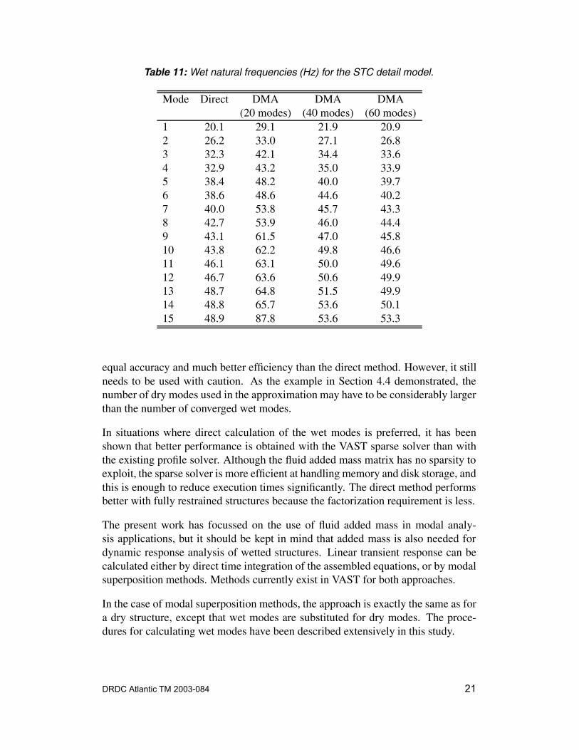
The wet natural frequencies for the direct method and DMA are given in Table 11.The DMA results are provided for three levels of approximation. Here, the numberof dry modes used in the approximation is considerably larger than the number ofconverged wet modes, and it is apparent that the convergence of the wet modes ismuch slower than was found in the previous examples. The slow convergence isdue to a large number of dry modes involving lateral vibration of the frames whichmake little contribution to the fifteen lowest wet modes. Unfortunately, it is notpossible to determine a priori which modes will be important to the approximationof the wet modes, and so many of the dry modes included may in fact be of littleinterest. If in this case a higher degree of accuracy is needed, the direct analysis ofthe wet modes may be the best option in spite of its larger computational cost.

With over 5500 panels on the wet surface, the added mass calculation for this modeltakes a little over twenty minutes using the modified code (Table 3). By contrast, thesame calculation with the existing method ran for over twenty-four hours withoutfinishing.

5 Conclusion

The work described in this study has resulted in significant improvement to DRDC’sfluid added mass and wet mode computational capability. Analyses that previouslytook several hours can now be performed in several minutes. The dry mode approx-imation for the wetted structural vibration modes has been shown to have nearly


Table 11: Wet natural frequencies (Hz) for the STC detail model.

Mode Direct DMA DMA DMA(20 modes) (40 modes) (60 modes)

1 20.1 29.1 21.9 20.92 26.2 33.0 27.1 26.83 32.3 42.1 34.4 33.64 32.9 43.2 35.0 33.95 38.4 48.2 40.0 39.76 38.6 48.6 44.6 40.27 40.0 53.8 45.7 43.38 42.7 53.9 46.0 44.49 43.1 61.5 47.0 45.810 43.8 62.2 49.8 46.611 46.1 63.1 50.0 49.612 46.7 63.6 50.6 49.913 48.7 64.8 51.5 49.914 48.8 65.7 53.6 50.115 48.9 87.8 53.6 53.3

equal accuracy and much better efficiency than the direct method. However, it stillneeds to be used with caution. As the example in Section 4.4 demonstrated, thenumber of dry modes used in the approximation may have to be considerably largerthan the number of converged wet modes.

In situations where direct calculation of the wet modes is preferred, it has beenshown that better performance is obtained with the VAST sparse solver than withthe existing profile solver. Although the fluid added mass matrix has no sparsity toexploit, the sparse solver is more efficient at handling memory and disk storage, andthis is enough to reduce execution times significantly. The direct method performsbetter with fully restrained structures because the factorization requirement is less.

The present work has focussed on the use of fluid added mass in modal analy-sis applications, but it should be kept in mind that added mass is also needed fordynamic response analysis of wetted structures. Linear transient response can becalculated either by direct time integration of the assembled equations, or by modalsuperposition methods. Methods currently exist in VAST for both approaches.

In the case of modal superposition methods, the approach is exactly the same as fora dry structure, except that wet modes are substituted for dry modes. The proce-dures for calculating wet modes have been described extensively in this study.


In the case of direct time integration methods, it should first be noted that, for drystructures, the VAST sparse solver was recently extended for use in direct linear andnonlinear time-integration calculations [2]. It turns out that the same algorithms thatwere developed for direct calculation of the wet modes can be re-used in direct time-integration calculations. This is analogous to the algorithm re-use that was achievedin the sparse solver developments for dry structures, as described in Reference [2].Thus the extension of the VAST sparse solver to time-integration analysis requiredlittle additional effort over what has already been described in this report.

References

1. Martec Limited. (2002). VAST – Vibration and Strength Analysis. Version 8.3User’s Manual.

2. Smith, M. J. (2002). A Sparse Solver for VAST. (DRDC Atlantic TM2002-140). DRDC Atlantic.

3. Vernon, T. A., Bara, B. and Hally, D. (1988). A Surface Panel Method for theCalculation of Added Mass Matrices for Finite Element Models. (DREA TM88/203). Defence Research Establishment Atlantic.

4. Golub, G. H., and Van Loan, C. F. (1989). Matrix Computations. Second Ed.Baltimore: The Johns Hopkins University Press.

5. Anderson, E., Bai, Z., Bischof, C., Blackford, S., Demmel, J., Dongarra, J., DuCroz, J., Greenbaum, A., Hammarling, S., McKenney, A., and Sorensen, D.(1999). LAPACK Users’ Guide, Third Ed. Philadelphia: Society for Industrialand Applied Mathematics.

6. Glenwright, D. G., and Hutton, S. G. (1987). Experimental and Finite ElementInvestigation of Added Mass Effects on Ship Structures. (DREA CR/87/464).Defence Research Establishment Atlantic.

7. Hutton, S. G., and Yang, J. (1990). Comparison of Added Mass Modeling forShips. (DREA CR/90/450). Defence Research Establishment Atlantic.


Annex AList of symbols, abbreviations, acronymsand initialisms

Symbols

�� diagonal matrix of fluid panel areas�� transformation between wet surface and structural nodal coordinates��, �� influence coefficient matrices�� identity matrix�� structural stiffness matrix�� structural mass matrix� number of dry modes�� fluid added mass matrix (in panel coordinates)�� fluid added mass matrix (in nodal coordinates) number of structural nodes on the wet surface total number of structural nodes� number of fluid panels� generalized structural displacement vector fluid panel source strength�� transformation matrix between fluid panel and nodal coordinates� structural displacement vector�� global Cartesian coordinates� shift parameter�� diagonal matrix of dry eigenvalues�� matrix of dry mode shapes�� wet mode shape

Abbreviations, acronyms and initialisms

DOF degree of freedomDMA dry mode approximationDRDC Defence R&D CanadaDSA detail stress analysisFEA finite element analysisflops floating point operationsISSMM Improved Ship Structure Maintenance ManagementIST ISSMM Software ToolRBM rigid body modeVAST Vibration and Strength Analysis




Date post:	10-Feb-2018
Category:	Documents
Upload:	ngoquynh
View:	221 times
Download:	1 times

Improved Added Mass and Wet Modes Calculation for Naval...

Documents