1

IMPROVED BONE DRILLING PROCESS THROUGH MODELING AND TESTING

By

KRITHIKA S PRABHU

A THESIS PRESENTED TO THE GRADUATE SCHOOL OF THE UNIVERSITY OF FLORIDA IN PARTIAL FULFILLMENT

OF THE REQUIREMENTS FOR THE DEGREE OF MASTER OF SCIENCE

UNIVERSITY OF FLORIDA

2007

2

© 2007 Krithika S. Prabhu

3

To my parents.

4

ACKNOWLEDGMENTS

I would like to thank my parents, Srikar and Vasudha Prabhu, for their love and

encouragement over my entire life. I thank my cousin Dr. Ganesh Rao for supporting me through

my graduate studies.

Special thanks go to my advisor, Dr. Tony Schmitz, for the advice and guidance

throughout my graduate studies. Also, thanks go to the other members of my committee, Dr.

John Schueller and Dr.Peter Ifju, for their support and involvement with this project.

A big thanks to all the members of the Machine Tool Research Center Lab for their advice and

help. I thank to Dr. Hahn and his student Leia Shanyfelt at the Laser-Based Diagnostic Laboratory

for their help with the laser ablation study.

5

TABLE OF CONTENTS page

ACKNOWLEDGMENTS ...............................................................................................................4

LIST OF TABLES...........................................................................................................................7

LIST OF FIGURES .........................................................................................................................8

ABSTRACT...................................................................................................................................10

CHAPTER

1 INTRODUCTION ..................................................................................................................12

2 LITERATURE SURVEY.......................................................................................................15

Parameters Influencing the Temperature Increase During Drilling .......................................16 Drill Rotational Speed .....................................................................................................16 Feed Rate .........................................................................................................................17 Drill Parameters...............................................................................................................17

Helix angle ...............................................................................................................17 Point angle................................................................................................................18 Drill diameter ...........................................................................................................18 Drill sharpness..........................................................................................................18 Flute..........................................................................................................................19 Irrigation...................................................................................................................19

Parameters Influencing the Drilling Force .............................................................................20 Force Temperature Correlation...............................................................................................20 Non Conventional Osteotomy (Bone Surgery) Methods........................................................21

Ultrasound Method..........................................................................................................21 Laser Method...................................................................................................................22 Pressurized Water Jet ......................................................................................................22

3 FINITE ELEMENT ANALYSIS ...........................................................................................25

Procedure ................................................................................................................................25 FE Model ................................................................................................................................25

Boundary Conditions.......................................................................................................25 Assumptions ....................................................................................................................26

Results.....................................................................................................................................26

4 EXPERIMENT DESCRIPTION............................................................................................37

Specimen and Preparation ......................................................................................................38 Sawbones.........................................................................................................................38 Bovine Bone ....................................................................................................................39

6

Experimental Equipment ........................................................................................................39 Experimental Procedure..........................................................................................................39

Sawbones Setup...............................................................................................................40 Bovine Bone Setup ..........................................................................................................40

5 RESULT AND DISCUSSION...............................................................................................49

Force Data...............................................................................................................................49 Temperature Data ...................................................................................................................51 Wear Study .............................................................................................................................51 Chip Formation.......................................................................................................................52 Hole Description.....................................................................................................................53

6 CONCLUSIONS AND DISCUSSIONS................................................................................67

7 FUTURE WORK....................................................................................................................69

APPENDIX

A LASER BONE ABLATION ..................................................................................................70

B MATLAB CODE....................................................................................................................75

LIST OF REFERENCES...............................................................................................................83

BIOGRAPHICAL SKETCH .........................................................................................................87

7

LIST OF TABLES

Table page 3-1 Bone material properties. ...................................................................................................35

3-2 Stress value for best, intermediate and worst case sequencing..........................................36

4-1 Description of drills. ..........................................................................................................48

5-1 Axial force results for sawbones........................................................................................64

5-2 Axial force results for bovine bone testing. .......................................................................64

5-3 Rank-ordered normalized axial force results for sawbones material.................................65

5-4 Rank-ordered axial force results for bovine bone testing. .................................................65

5-5 Temperature results and chip type for sawbones...............................................................66

5-6 Temperature results and chip type for bovine bone testing. ..............................................66

A-1 Laser ablation parameters for the holes. ............................................................................74

8

LIST OF FIGURES

Figure page 1-1 Figure showing the cancellous and cortical (compact) part of bone. ................................14

2-1 Drill geometry....................................................................................................................24

3-1 Setup showing work-piece bolted to aluminum fixture.....................................................28

3-2 Picture of the sawbones work-piece with the 16 holes. .....................................................29

3-3 Work-piece showing the hole numbering. .........................................................................30

3-4 Classification of holes based on stress...............................................................................31

3-5 Stress distribution during drilling of last hole of the best case. .........................................32

3-6 Stress distribution during drilling of first hole of the worst case.......................................33

3-7 Stress at each hole for best, intermediate and worst case. .................................................34

4-1 Drill wandering and surface preparation using an end mill ...............................................42

4-2 Bone work-piece before milling. .......................................................................................43

4-3 Bone work-piece with its drilling surface flattened by milling. ........................................44

4-4 Picture of the drills with reference number........................................................................45

4-5 Photograph of drilling setup...............................................................................................46

4-6 Photograph of drilling setup showing bone sample, vise, and drill/chuck. .......................47

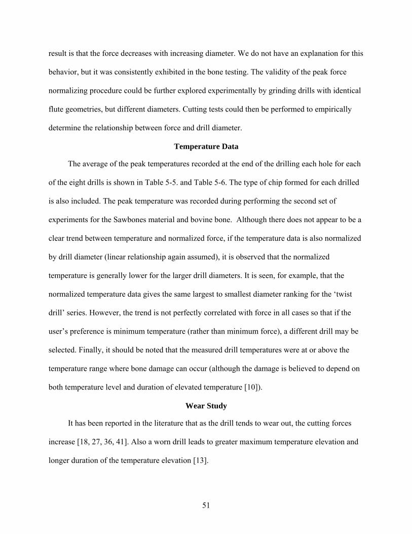
5-1 Drill setup showing the direction of positive X, Y and Z axis. .........................................54

5-2 Sample force result for Sawbones material showing X, Y and Z forces. ..........................55

5-3 Sample force result for bovine bone showing X, Y and Z forces......................................56

5-4 Peak axial drilling force as a function of drill diameter for ‘twist drill’ series with no normalization. ....................................................................................................................57

5-5 Photograph of the twist drills with reference number........................................................58

5-6 Axial drilling force versus drill hole number for Sawbones material wear study. ............59

5-7 Axial drilling force versus drill hole number for bovine bone wear study........................60

9

5-8 Continuous chip in case of Sawbones material..................................................................61

5-9 Sample chips obtained from 210444 drill. .........................................................................62

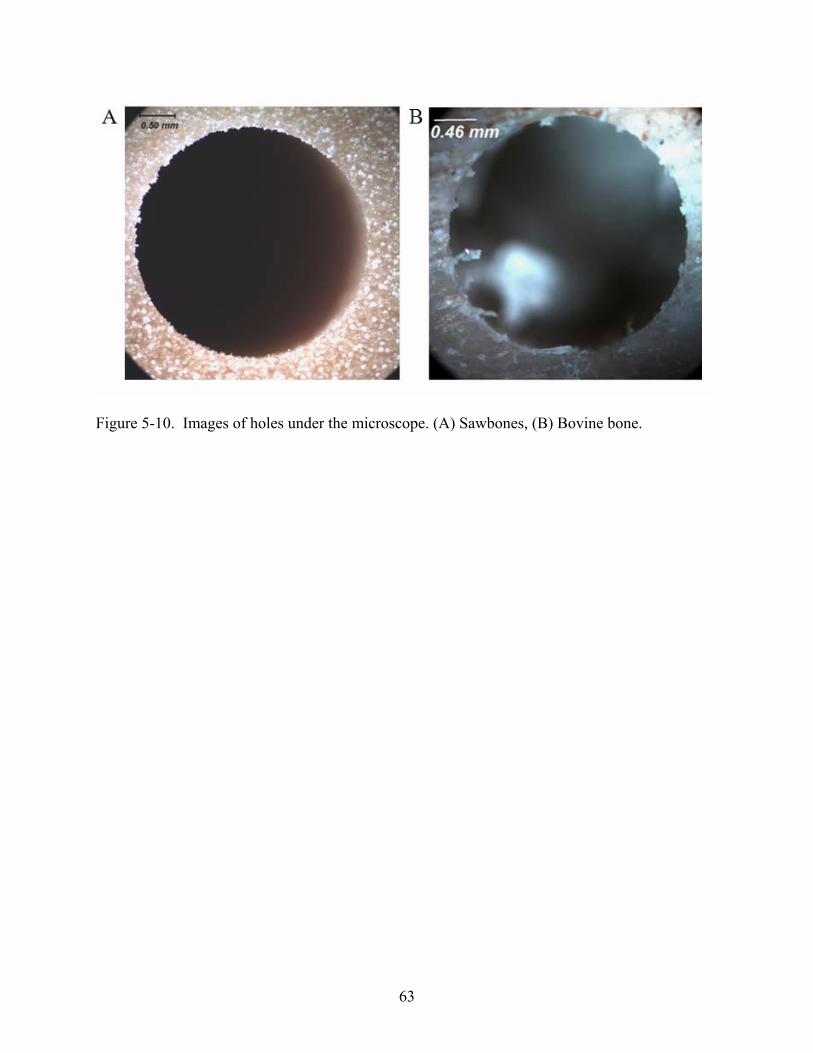
5-10 Images of holes under the microscope...............................................................................63

A-1 Laser ablation setup. ..........................................................................................................71

A-2 Microscopic image of the bone work-piece under 1x magnification. ...............................72

A-3 Example holes in bovine bone sample by mechanical drilling and laser ablation.............73

10

Abstract of Thesis Presented to the Graduate School of the University of Florida in Partial Fulfillment of the

Requirements for the Degree of Master of Science

IMPROVED BONE DRILLING PROCESS THROUGH MODELING AND TESTING

By

Krithika S. Prabhu

December 2007

Chair: Tony L. Schmitz Major: Mechanical Engineering

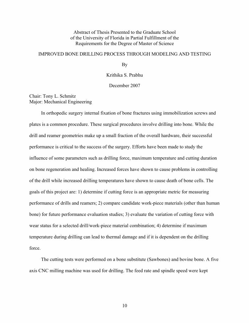
In orthopedic surgery internal fixation of bone fractures using immobilization screws and

plates is a common procedure. These surgical procedures involve drilling into bone. While the

drill and reamer geometries make up a small fraction of the overall hardware, their successful

performance is critical to the success of the surgery. Efforts have been made to study the

influence of some parameters such as drilling force, maximum temperature and cutting duration

on bone regeneration and healing. Increased forces have shown to cause problems in controlling

of the drill while increased drilling temperatures have shown to cause death of bone cells. The

goals of this project are: 1) determine if cutting force is an appropriate metric for measuring

performance of drills and reamers; 2) compare candidate work-piece materials (other than human

bone) for future performance evaluation studies; 3) evaluate the variation of cutting force with

wear status for a selected drill/work-piece material combination; 4) determine if maximum

temperature during drilling can lead to thermal damage and if it is dependent on the drilling

force.

The cutting tests were performed on a bone substitute (Sawbones) and bovine bone. A five

axis CNC milling machine was used for drilling. The feed rate and spindle speed were kept

11

constant. The axial force was measured using a three component dynamometer and the

maximum temperature was measured using a K-type thermocouple.

Results showed that for force comparison, the Sawbones material provided a reasonable

replacement for bone. Wear is not a primary issue for a reasonable number of holes per drill.

Also drill point temperature measurements showed levels which could lead to bone damage for

the selected cutting conditions. But there was no clear correlation seen between the drilling force

and maximum temperature. There were clear force differences between drill geometries with the

same diameter and the force per unit diameter was generally lower for larger diameter drills. A

mechanistic model of drilling force based on the geometry which quantifies the effect of changes

in drill geometry on force remains an area for future work.

12

CHAPTER 1 INTRODUCTION

Bone fracture has been a problem for a while. It is important to return the fracture parts

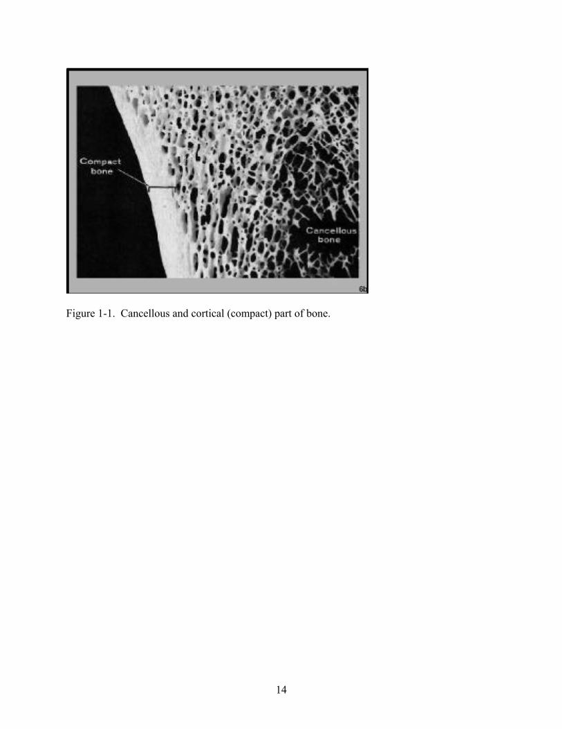
into their initial position and fixate them. Bone is made up of inter-cellular calcified material. It

has an outer hard layer called the cortical bone and inner spongy later called cancellous bone as

shown in Figure 1-1. The outer surface of the bone is covered by tough layer called the

periosteum while the inner surface is lined by endosteum. When bone is broken these two layers

provide bone forming cells which helps in bridging the fracture. Adequate stabilizing of the

fracture fragments of bone until healing occurs is crucial. This can be done by immobilization of

the fractured parts or by drilling the bone around the fracture site and setting immobilization

screws, plates and/or wires and perform bone fixation [1-3]. Power tools like burs, ultrasonic

cutters, chisels, drills and saws are used for these purposes [4]. Drilling is the most widely used

preliminary step in insertion of pins or screws during repair of fractures or installation of

prosthetic device. It is also the most difficult to satisfactorily perform [5].

The various requirements to satisfy the orthopedic surgery are rapid cutting to minimize

operating time, relative ease of instrument control for the surgeon, rapid bone regeneration,

reduction in thermal tissue damage, precision, reduction in loss of bone tissue and its dispersion

into operating area [6]. The success of the orthopedic fixation devices depend partially on the

quality and quantity of the host bone. The traumatologist needs to apply pressure on the drilling

tool in order to ensure uniform penetration of the drill through the bone. This results in

temperature increase caused by plastic deformation of the bone chips and friction between the

drill tool and the bone. When the temperature of the bone is raised above 47°C thermal necrosis

of the bone occurs due to irreversible death of the bone cells. This has adverse effects on bone

regeneration and healing [1, 7-12].

13

Increased force during penetration causes poor control of the drill, uncontrolled bursting

through cortex or drill breakage [11]. New mechatronic drills using the cutting force information

are used to assist surgeons during the cutting intervention [13]. Also there are other problems

during trauma surgery such as drill hole accuracy, maintaining free hand control even when

using drill guide, drill walking and unpredictable situation due to non-homogeneity of the bone

material [3, 5, 6].

Reaming is performed to finish the drilled hole. It increases the contact area between the

bone and the implant and makes the drilled passage more uniform. It helps in providing a more

stable fixation and allowance for the use of larger and stronger implants that are less likely to fail

by fatigue. It also promotes healing by creating grafts at the fracture site. Typically the

temperature increase due to reaming does not exceed the limits that would produce bone

necrosis. The reason being that reaming process typically does not take more than forty seconds.

The average contact time during reaming is around fifteen seconds. Hence even if the

temperature goes around 70°C it would not result in necrosis [14].

14

Figure 1-1. Cancellous and cortical (compact) part of bone.

15

CHAPTER 2 LITERATURE SURVEY

In orthopedic surgery high-speed cutting tools are often applied to bone. Mechanized

cutting tools such as drills produce heat which raises the temperature of both the tool and the

material. Bone has a low thermal diffusivity which is in the region of 0.1 cm2/s as compared to

9.43 cm2/s for Titanium [3]. Hence, the heat generated is of particular concern in these

operations because the heat generated during drilling is not dissipated quickly but remains

around the drilled holes. Studies have shown that, if the temperature of the bone is raised above a

threshold thermal necrosis will ensue. The duration of exposure to elevated temperature has a

significant influence on the amount of damage done [15].

Hence it is important to keep temperatures below this threshold since thermal necrosis can

have a negative impact on the outcome of surgical drilling procedures. For example, operations

that require rigid fixation of pins can fail because the implants become encapsulated by soft

tissue instead of new bone if the bone matrix around the pin is damaged. Postoperative

complications such as infections and loosening in the necrotic bone surrounding the pin insertion

site after the pins were removed can occur. Even though strong external skeletal fixation frame

units are used the loosening of pins can cause detrimental effects [2]. Furthermore, fractures can

occur across the pin insertion defects. There can be failure due to an increase in resorption of

bone from around the drilled bone. Also delay in healing is associated with elevated cortical

temperatures [2, 8, 9, 16-18]. These problems arise because the mechanical properties of the

living bone are altered by overheating [8, 9]. Dehydration, desiccation, shrinkage and

carbonization of the bone occur due to high temperature which causes the cell metabolism to halt

[15].

16

Although the problem has been investigated many times through experiment, conflicting

results were produced, leading to disagreement in the proper approach to surgical drilling.

Literature review reveals that temperature recorded for bone drilling varies considerably. This

inconsistency may be probably due to variation in experimental conditions from one test case to

another. Surgical parameters such as drill geometry, drill wear, drill speed, applied pressure,

irrigation, etc, vary in each case [19].

For example, holes were drilled into bone specimens from a variety of species and

anatomical locations for the purpose of determining the thermal impact of the drill rotational

speed. Significant difference is seen between physical properties of different bones and separate

regions in the same bone. Bone is a heterogeneous anisotropic material [20-22]. Variation in

bone mineralization, collagen content and orientation as well as the degree of collagen cross-

linking influences its mechanical properties [23]. In some cases force is applied during drilling.

This in turn affects the temperature increase during drilling. Also there is irrigation in some cases

in form of water or forced air and some cases there is no irrigation. Different cutting tools are

employed and feed rates are also varied [10].

Parameters Influencing the Temperature Increase During Drilling

Drill Rotational Speed

There has been no consistent trend reported for the effect of drill rotation speed on heat

production. Some show an increase in temperature with increasing speed whereas some show a

decrease [10].

A trend in decreasing temperature by increasing the drill axial speed has been reported by

some. In this case, the time required for drilling is reduced due to increased speed of penetration.

This in turn reduces the temperature as heat penetrates for a lesser amount of time. If the duration

of temperature above critical values is less than 1 minute, there is no thermal necrosis. For

17

human bone this threshold is 47 °C for 1 minute [16]. Some studies show that tissue damage is

avoided at speeds above 200,000 rpm [1, 7, 16]. Microscopic examination has shown less initial

inflammatory response, smoother cut edge, and faster recovery in case of ultra speed drilling

[24].

However an increasing trend has been reported in some citations. It has been reported that

the maximum temperature and resultant thermal damage increases with drill rotational speed.

This is true in the range of 400 rpm to 10,000 rmp [25]. There is a significant softening of the

bone at higher rotational speed indicated by lower shear stress value. Hence the drill rotational

speed should be reduced as much as possible [1, 2, 10, 16, 26-28]. But as the rotation speed is

increased above 10,000 rpm there is a decreasing trend observed until 24,000 rpm after which it

is constant [25]. Though at lower speeds the edge of the drilled hole was not clearly cut and there

was lower degree of circularity [28]. Some have reported no influence of drill rotation speed on

temperature [8]. It is recommended to drill in the speed range of 750-1250 rpm to take the

advantage of the decrease in the flow stress of the material at these speeds [26].

Feed Rate

There is an inverse relation of drilling temperature with feed rate. As the feed rate

increases the time required for drilling reduces and hence there is shorter time of friction

between the drilling tool and the bone with a consequent lower drilling temperature [1].

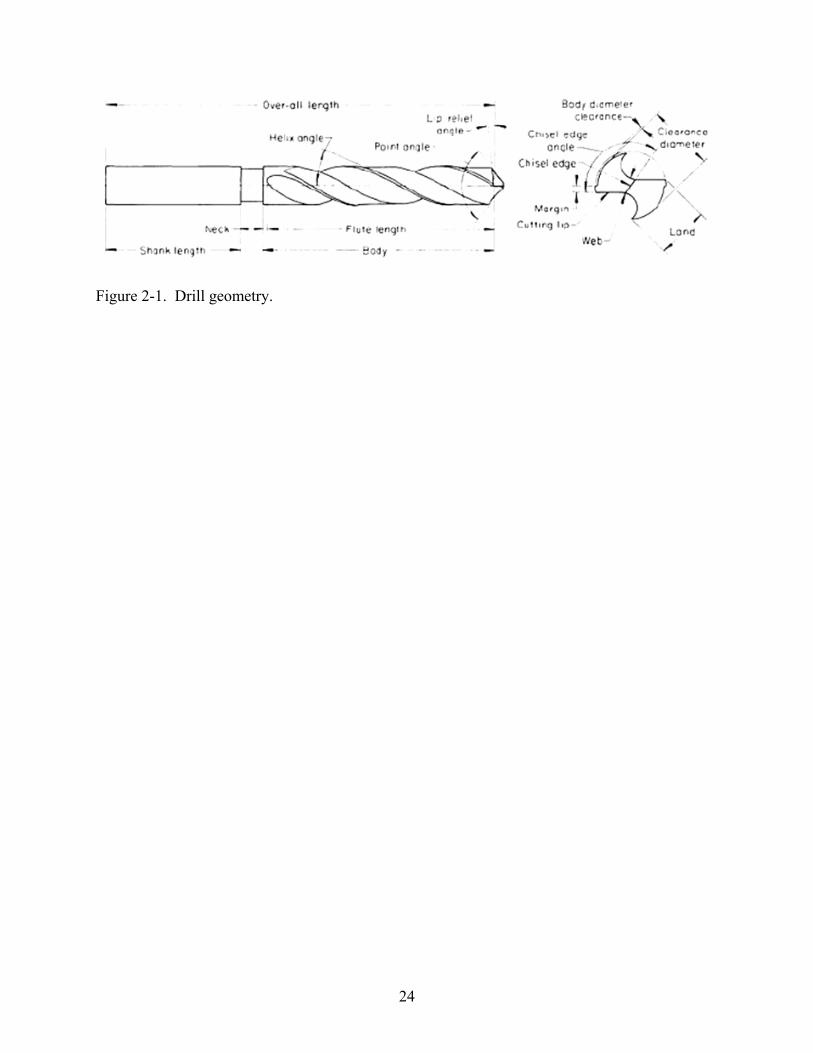
Drill Parameters

Figure 2-1. shows the drill geometry. The influence of the drill parameters are mentioned

below.

Helix angle

The helix angle of the drill influences the temperate rise during drilling. The helix angle of

a drill bit varies with the drill diameter; larger angles are used for larger diameter drills. The

18

optimum range for the helix angle has been reported as 24–36° [12]. Usually most standard

orthopedic drills have a slow helix angle. This geometry is ideal in case of drilling into dry bone

as there is short chipping and the debris is cleared off easily. But in vitro case, the debris is wet

and mixed with medullar fat, hence a theoretical a quick helix angle would be more efficient in

clearing the debris [11].

Point angle

It is not possible to locate a flat surface while drilling into the bone. Using a drill guide is

not always possible. Hence the surgical drill must be self centering and it should not walk while

initiating a hole in the cortex of a long bone. An optimum point angle is desirable to prevent drill

from walking on the surface [26]. For standard orthopedic drills it is 90° as it leads to lower

temperatures during drilling. The periosteum obstructs the chip flow through the drill flutes. The

chisel edge of the drill catches the periosteum and eventually carries it to the flutes where it

obstructs the chip flow. A spilt point design offers a solution to this problem by imparting a

positive rake angle and cutting action to the chisel edge. Theoretically a split point reduces the

friction and in turn the heat generated [11]. Larger helix and point angles impart a positive rake

angle for a greater proportion of the cutting lip. This improves bone drill efficiency [3].

Drill diameter

The maximum temperature increases with drill diameter.

Drill sharpness

Blunt drill bits are reported to produce more thermal damage [6, 11, 27, 29]. A worn tool

causes greater maximum temperature elevation and longer duration of temperature elevation. In

the case of reaming, worn reamers has been shown to produce higher temperatures of about 10°C

higher than sharper reamers [19].

19

Flute

After removal of bone by formation of chips, it is necessary to remove the chips from the

cutting zone while the drill continues to penetrate. This requires that the chip material from each

major cutting edge should follow the spiral path up along the flutes to the work piece surface.

The flutes may clog when the depth of the hole being drilled becomes appreciable to the

diameter thus leading to a substantial increase in the torque and specific cutting energy. This

leads to significant increase in temperature. Bone chips in the flutes exert a pressure against the

internal surface of the hole being drilled and friction at this interface gives rise to a

circumferential shear traction stress. Also there is very limited access for the irrigation fluid.

Drill flute geometry has a significant effect upon the ease with which the bone chips are

extracted from the cutting zones during drilling [13, 22]. Flutes for surgical drills have

traditionally been helical with U grooves. Parabolic flute design has proved to be effective in

ejecting and smoothly removing bone chips from the cutting zone, especially when the length of

the hole was 5–6 times the drill diameter [4]. Also temperature is lower in case of a two phase

drill as compared to a classical surgical drill. This is because in the former case the bone is pre

drilled with a smaller diameter drill [1].

Irrigation

The thermal damage is influenced by irrigation. Usage of coolant reduces the temperature

during drilling [6, 28, 30]. Water coolant and internal irrigation is shown to reduce the frictional

heat [31]. Coolant sprayed on the cutting tool decreases the temperature but does not completely

prevent a temperature change in the bone [15, 27].

In case of reaming, room temperature saline is shown to reduce the cortical bone

temperature. It is effective even in the case of single pass reaming is more aggressive than

stepwise reaming [32].

20

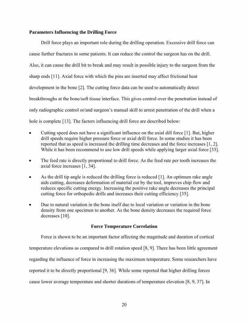
Parameters Influencing the Drilling Force

Drill force plays an important role during the drilling operation. Excessive drill force can

cause further fractures in some patients. It can reduce the control the surgeon has on the drill.

Also, it can cause the drill bit to break and may result in possible injury to the surgeon from the

sharp ends [11]. Axial force with which the pins are inserted may affect frictional heat

development in the bone [2]. The cutting force data can be used to automatically detect

breakthroughs at the bone/soft tissue interface. This gives control over the penetration instead of

only radiographic control or/and surgeon’s manual skill to arrest penetration of the drill when a

hole is complete [13]. The factors influencing drill force are described below:

• Cutting speed does not have a significant influence on the axial dill force [1]. But, higher drill speeds require higher pressure force or axial drill force. In some studies it has been reported that as speed is increased the drilling time decreases and the force increases [1, 2]. While it has been recommend to use low drill speeds while applying larger axial force [33].

• The feed rate is directly proportional to drill force. As the feed rate per tooth increases the axial force increases [1, 34].

• As the drill tip angle is reduced the drilling force is reduced [1]. An optimum rake angle aids cutting, decreases deformation of material cut by the tool, improves chip flow and reduces specific cutting energy. Increasing the positive rake angle decreases the principal cutting force for orthopedic drills and increases their cutting efficiency [35].

• Due to natural variation in the bone itself due to local variation or variation in the bone density from one specimen to another. As the bone density decreases the required force decreases [10].

Force Temperature Correlation

Force is shown to be an important factor affecting the magnitude and duration of cortical

temperature elevations as compared to drill rotation speed [8, 9]. There has been little agreement

regarding the influence of force in increasing the maximum temperature. Some researchers have

reported it to be directly proportional [9, 36]. While some reported that higher drilling forces

cause lower average temperature and shorter durations of temperature elevation [8, 9, 37]. In

21

recent studies, Abouzgia and James have reported a temperature rise with force to a certain point

and then a fall with greater force. This rise and fall of temperature with force is attributed to

competing factors such as the rate of heat generation and the duration. The product of these two

factors is the total heat generated. Since the rate of heat increases with load while the duration

decreases, the resultant product varies. Ideally the heat should increase as the force increases

from zero, which is the case initially. But as the force increases to higher values, the temperature

decreases indicating that the duration is the dominant factor among the two.

These conflicts in results could be attributed to difference in the drill speed range and the

force applied while drilling. The drill speed reported is the free-running (manufacturer's listed

speed) speed which is assumed to be the speeds during drilling. Though, it is shown that the

speed of an electrically powered drill is dependent on the applied force and the differences are as

high as 50% between operating speed (speed under load) and free-running speed [36].

Non Conventional Osteotomy (Bone Surgery) Methods

There are disadvantages of mechanical method of drilling in to bone such as cracking and

splintering of bone rotation, thermal damage due to vibration and spread of bone particles in the

surrounding area [38]. This has motivated researchers to look into alternative methods. Since

bone is a composite material, industrial machining techniques such as ultra sonic devices, lasers

or pressurized jets used for machining composites can be used for machining it [6].

Ultrasound Method

Ultrasound devices have been used for bone surgery. But usage of coolant to dissipate heat

is strongly recommended. The healing response in this case is comparable to the conventional

method. The primary advantages of this method are maneuverability at the surgical sites which

limits the risks of damaging the adjacent tissues, precision, hemorrhage control and uneventful

healing with an absence of post operative sequel. The cut surfaces are reported to be smoother

22

than conventional methods and the necrosed zones are sufficiently small not to affect

regeneration. It is useful when the object is small and high precision is required [6, 39-41]. The

main disadvantage of this method is the prolonged cutting time leading to high temperature rise,

lack of knowledge concerning the long term effects and fatigue failure of osteotome parts [6, 40].

To overcome the problem of thermal damage ultra sound surgical instruments employing peizo-

electric materials are used. Ultra sonic vibrations are used to perform operations. In this method

the frequency can be regulated in order to control the temperature [41]. Hence this method offers

the advantage of a haemostatic effect at the level of the cut surface, precision, and temperature

control. However this method is restricted to shallow cuts [42].

Laser Method

The main advantages are reduced operative field, enhanced maneuverability, limited

damage to surrounding issue, reduced operation time, cauterization effect, absence of physical

contact and simulation of granulation tissue. CO2 lasers are usually used for cutting bone. In this

method, the target surface absorbs a large quantity of energy which causes ablation of the bone

fragment by photodecomposition. The main disadvantage of this method is that the thermal

necrosis threshold is exceeded. This leads to a delay in healing after use of laser [6].

Pressurized Water Jet

In this method water is brought to very high pressure, of the order of 108 Pa, and then

directed onto the cutting area where it is expelled through an orifice with a small cross section,

less than a square millimeter. It is thus possible to cross through the cortical wall of a dry

femoral bone and obtain an extremely fine cutting line. Furthermore, there does not appear to be

any significant temperature rise at the level of the cutting surface. However there are certain

problems encountered to its use in surgery. If the cortical part of the bone is cut, control of the jet

is lost at the medullar level and can cause serious damage. Given the power of the jet, if it is not

23

directed onto the bone structure, there is a risk of damaging the surrounding tissue. But with

improvements, such as jet control and pressure optimization, this technique could be of interest

in surgical fields [6].

24

Figure 2-1. Drill geometry.

25

CHAPTER 3 FINITE ELEMENT ANALYSIS

Finite Element Analysis is used in order to determine an optimum sequence for drilling

holes. Sequencing is done in a fashion so as to reduce the maximum stresses induced in the work

piece.

Procedure

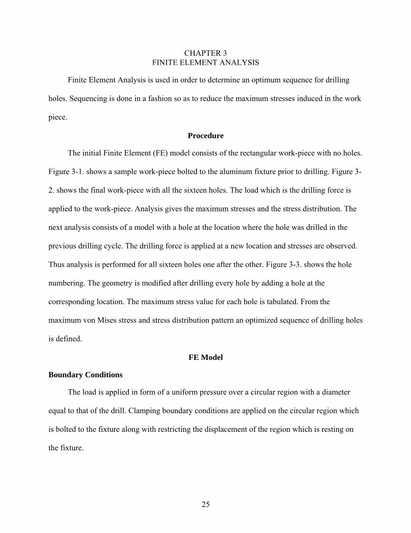
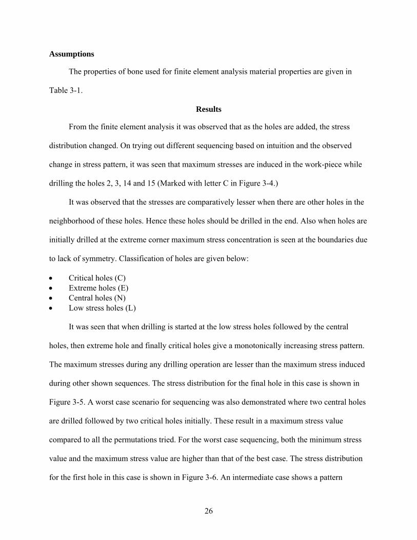
The initial Finite Element (FE) model consists of the rectangular work-piece with no holes.

Figure 3-1. shows a sample work-piece bolted to the aluminum fixture prior to drilling. Figure 3-

2. shows the final work-piece with all the sixteen holes. The load which is the drilling force is

applied to the work-piece. Analysis gives the maximum stresses and the stress distribution. The

next analysis consists of a model with a hole at the location where the hole was drilled in the

previous drilling cycle. The drilling force is applied at a new location and stresses are observed.

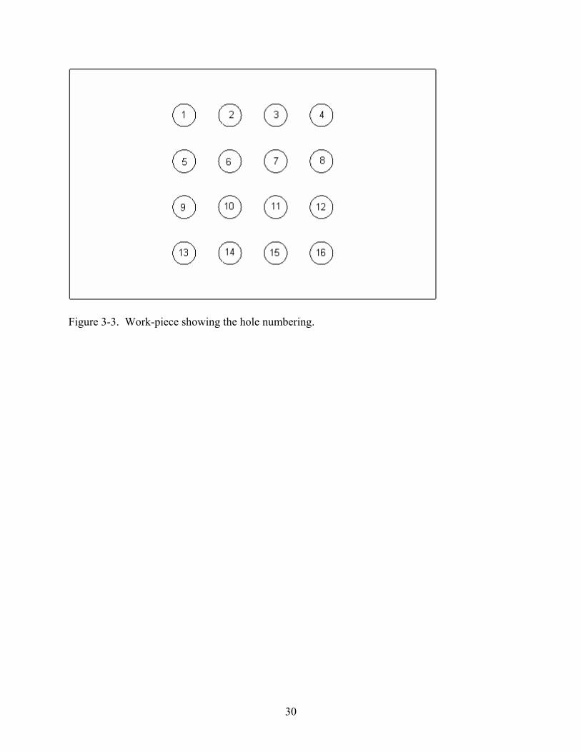
Thus analysis is performed for all sixteen holes one after the other. Figure 3-3. shows the hole

numbering. The geometry is modified after drilling every hole by adding a hole at the

corresponding location. The maximum stress value for each hole is tabulated. From the

maximum von Mises stress and stress distribution pattern an optimized sequence of drilling holes

is defined.

FE Model

Boundary Conditions

The load is applied in form of a uniform pressure over a circular region with a diameter

equal to that of the drill. Clamping boundary conditions are applied on the circular region which

is bolted to the fixture along with restricting the displacement of the region which is resting on

the fixture.

26

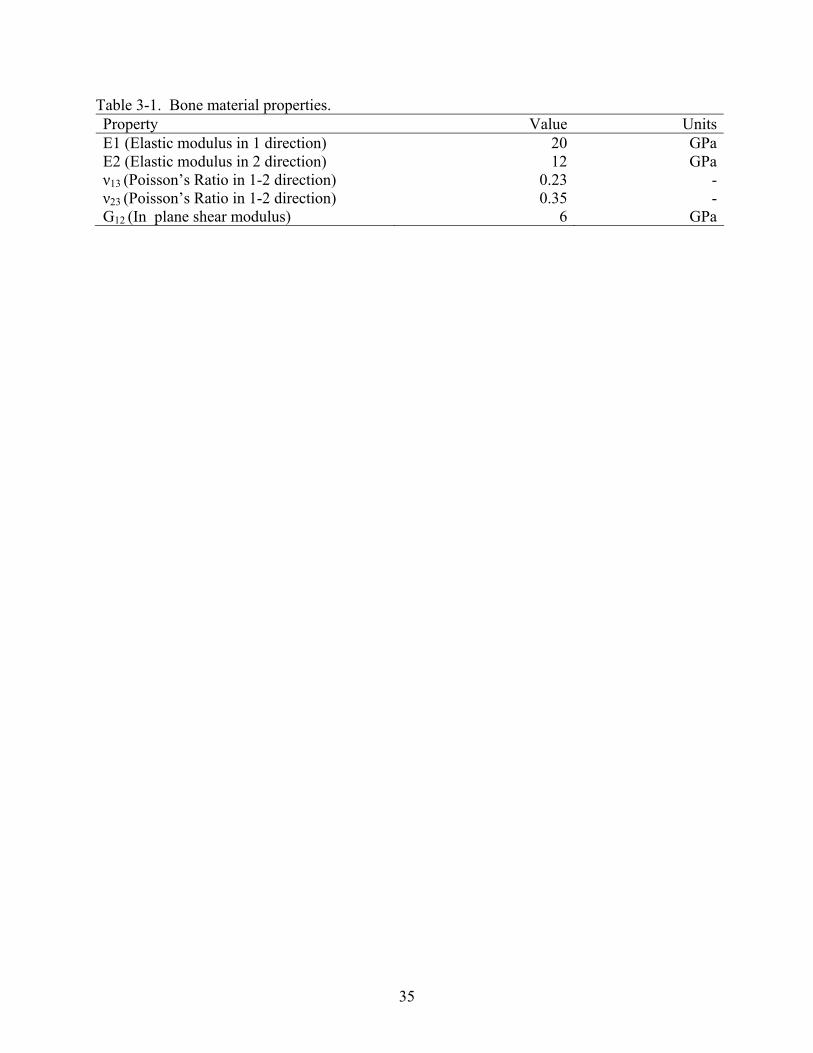
Assumptions

The properties of bone used for finite element analysis material properties are given in

Table 3-1.

Results

From the finite element analysis it was observed that as the holes are added, the stress

distribution changed. On trying out different sequencing based on intuition and the observed

change in stress pattern, it was seen that maximum stresses are induced in the work-piece while

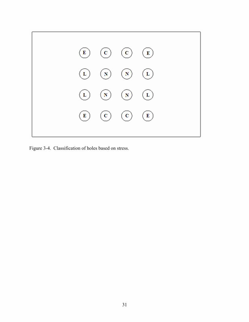
drilling the holes 2, 3, 14 and 15 (Marked with letter C in Figure 3-4.)

It was observed that the stresses are comparatively lesser when there are other holes in the

neighborhood of these holes. Hence these holes should be drilled in the end. Also when holes are

initially drilled at the extreme corner maximum stress concentration is seen at the boundaries due

to lack of symmetry. Classification of holes are given below:

• Critical holes (C) • Extreme holes (E) • Central holes (N) • Low stress holes (L)

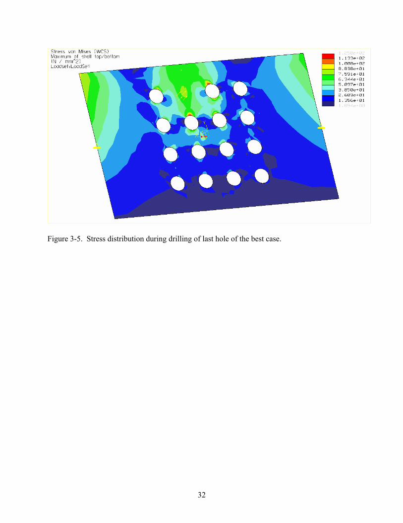
It was seen that when drilling is started at the low stress holes followed by the central

holes, then extreme hole and finally critical holes give a monotonically increasing stress pattern.

The maximum stresses during any drilling operation are lesser than the maximum stress induced

during other shown sequences. The stress distribution for the final hole in this case is shown in

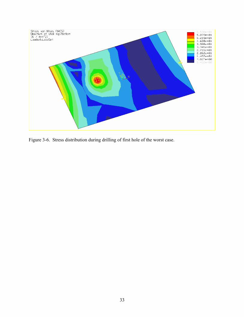
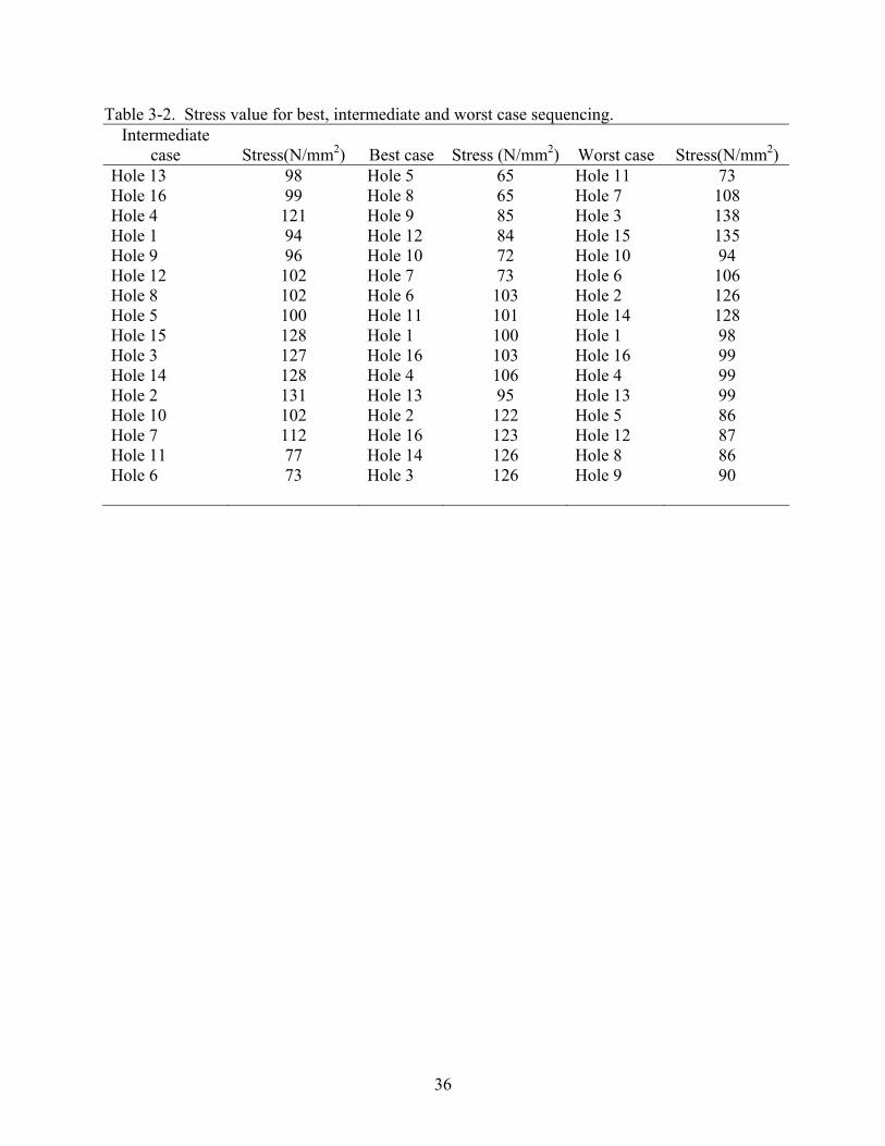
Figure 3-5. A worst case scenario for sequencing was also demonstrated where two central holes

are drilled followed by two critical holes initially. These result in a maximum stress value

compared to all the permutations tried. For the worst case sequencing, both the minimum stress

value and the maximum stress value are higher than that of the best case. The stress distribution

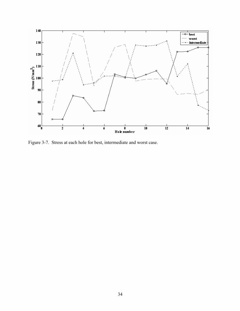
for the first hole in this case is shown in Figure 3-6. An intermediate case shows a pattern

27

between the best and worst case. The stress values for the best, intermediate and worst cases are

shown in Table 3-2. and the trend for each case is plotted against hole number in Figure 3-7.

An experimental validation of this analysis has not been performed.

28

Figure 3-1. Setup showing work-piece bolted to aluminum fixture.

29

Figure 3-2. Picture of the sawbones work-piece with the 16 holes.

30

Figure 3-3. Work-piece showing the hole numbering.

31

Figure 3-4. Classification of holes based on stress.

32

Figure 3-5. Stress distribution during drilling of last hole of the best case.

33

Figure 3-6. Stress distribution during drilling of first hole of the worst case.

34

Figure 3-7. Stress at each hole for best, intermediate and worst case.

35

Table 3-1. Bone material properties. Property Value UnitsE1 (Elastic modulus in 1 direction) 20 GPaE2 (Elastic modulus in 2 direction) 12 GPaν13 (Poisson’s Ratio in 1-2 direction) 0.23 -ν23 (Poisson’s Ratio in 1-2 direction) 0.35 -G12 (In plane shear modulus) 6 GPa

36

Table 3-2. Stress value for best, intermediate and worst case sequencing. Intermediate

case Stress(N/mm2) Best case Stress (N/mm2) Worst case Stress(N/mm2) Hole 13 98 Hole 5 65 Hole 11 73 Hole 16 99 Hole 8 65 Hole 7 108 Hole 4 121 Hole 9 85 Hole 3 138 Hole 1 94 Hole 12 84 Hole 15 135 Hole 9 96 Hole 10 72 Hole 10 94 Hole 12 102 Hole 7 73 Hole 6 106 Hole 8 102 Hole 6 103 Hole 2 126 Hole 5 100 Hole 11 101 Hole 14 128 Hole 15 128 Hole 1 100 Hole 1 98 Hole 3 127 Hole 16 103 Hole 16 99 Hole 14 128 Hole 4 106 Hole 4 99 Hole 2 131 Hole 13 95 Hole 13 99 Hole 10 102 Hole 2 122 Hole 5 86 Hole 7 112 Hole 16 123 Hole 12 87 Hole 11 77 Hole 14 126 Hole 8 86 Hole 6 73 Hole 3 126 Hole 9 90

37

CHAPTER 4 EXPERIMENT DESCRIPTION

The variable factors involved in orthopedic surgery include the type of bone, drill

geometry, rotational speed of the drill, force applied while drilling, duration of drilling, use of

coolant, and variation between operators, among others. From the range of drills available for

bone drilling, eight different drills were selected. Because the majority of the drills were very

long and the intent of this study was to understand the relationship between drill geometry and

force levels (independent of dynamic effects due to drill flexibility), all drills were cut to an

equal length.

The drilling tests were performed to compare the peak axial force for the different drill

geometries. Hence the feed per revolution and the spindle speed were maintained at constant

levels.

The properties of human bone vary from site to site within the body, with the age of the

person, and due to any pathological processes that may have occurred. It is difficult to obtain

fresh human bone in quantities required for significant experimental testing. Hence initial

experiments were performed using a bone substitute, Sawbones©, which is widely used in

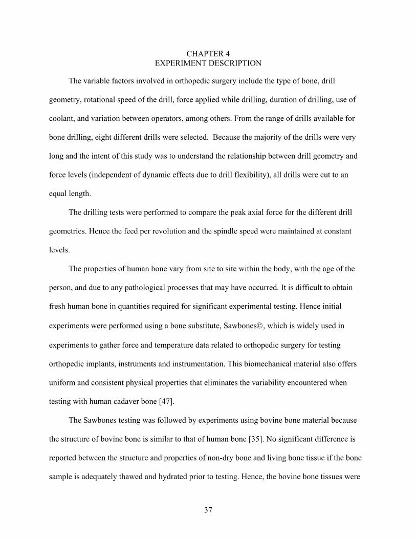
experiments to gather force and temperature data related to orthopedic surgery for testing

orthopedic implants, instruments and instrumentation. This biomechanical material also offers

uniform and consistent physical properties that eliminates the variability encountered when

testing with human cadaver bone [47].

The Sawbones testing was followed by experiments using bovine bone material because

the structure of bovine bone is similar to that of human bone [35]. No significant difference is

reported between the structure and properties of non-dry bone and living bone tissue if the bone

sample is adequately thawed and hydrated prior to testing. Hence, the bovine bone tissues were

38

kept in cold storage [12, 45]. Also, for cortical bone there not a significant difference in the

energy absorbed to failure and maximum stress at room temperature (21°) and body temperature

(37°) [12]. The experiments were therefore carried out at room temperature.

Differences in cortical thickness can influence the drilling temperature. There is a strong

correlation between the cutting depth and heat generation [13]. Using samples of uniform

thickness, each drill removed the same depth of cortical material over an identical time period

prior to temperature measurement (completed using a contact thermocouple probe applied to the

drill tip immediately after exiting the material). It was believed that this was important to enable

temperature comparisons between individual drill geometries. The majority of the holes drilled

into bones for insertion of screws are made in the shaft of the long bones [46]. The material

properties are less consistent at bone ends [47]. Therefore, the samples were taken from the

center portion of the shaft of each bone. Also, the drilling direction was always radial (toward the

bone center) due to the anisotropic material behavior of bone and material from the bone ‘shank’

(away from the ends) was used because the material properties are less consistent at the bone

ends [1].

Specimen and Preparation

The specimen preparation procedure for Sawbones and bovine bone material has been

specified below.

Sawbones

Samples of the Sawbones material were prepared in the form of blocks with dimensions of

80 mm x 44 mm x 10 mm. For this, first the Sawbones material blocks were sectioned using a

band saw. The sectioned test blocks were then finished machined.

39

Bovine Bone

The bone specimens were prepared by sectioning the femur along its long axis using a

band saw. Two specimens were taken from the medial and lateral quadrants of the mid-

diaphysis. The cross section of the bone samples were measured before machining [12]. The

specimens were about 107.2 mm in length, 71 mm in width and 30.7 mm in depth. The average

depth of the cortical portion was 7.5 mm. All soft tissue was stripped from the specimen to clear

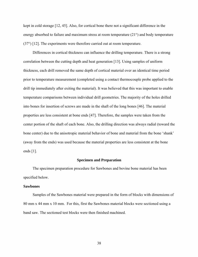
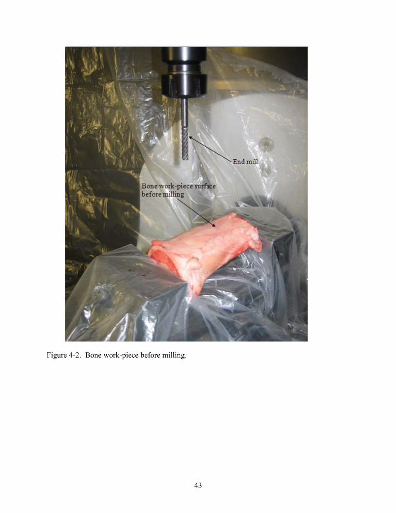
the surface. This included the periosteum. Furthermore, since the samples in this case did not

have a regular shape, an end-mill was used to prepare a flat surface perpendicular to the drill axis

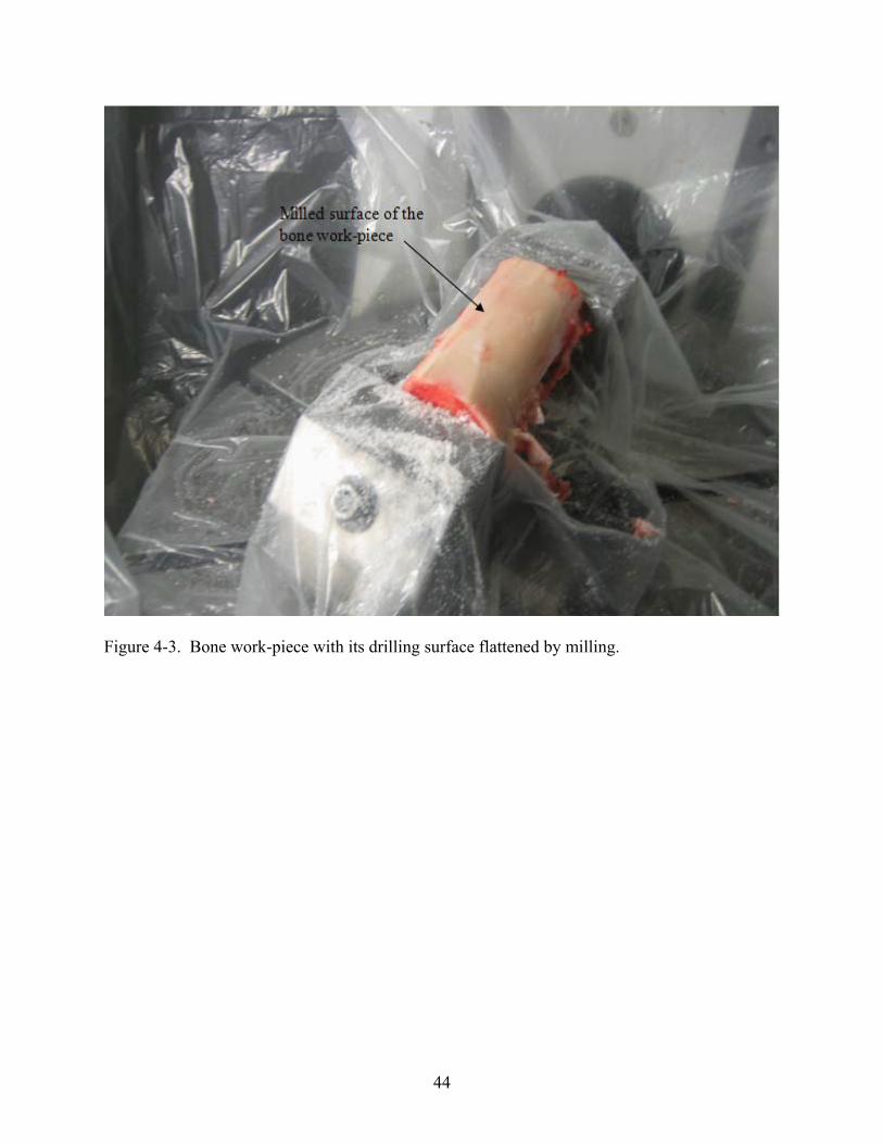
prior to carrying out the drilling tests. This is demonstrated schematically in Figure 4-1. The

bone work-piece prior to facing is shown in Figure 4-2. The milled surface is shown in Fig. 4-3.

Experimental Equipment

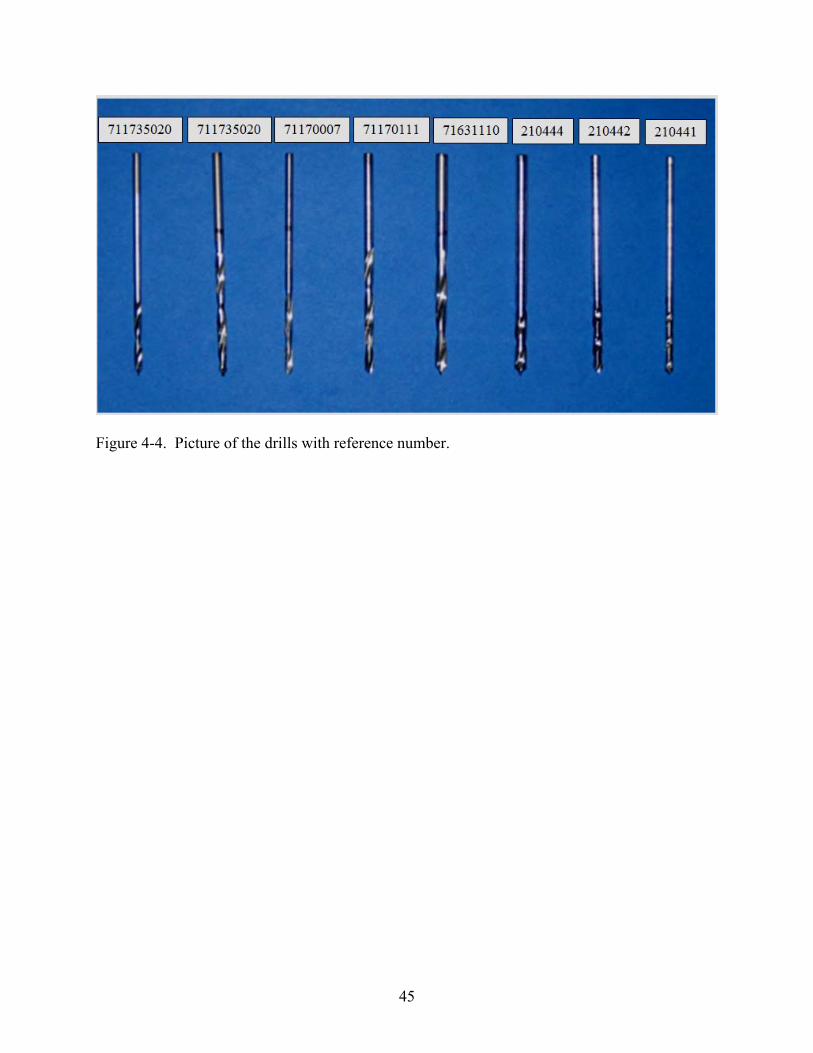
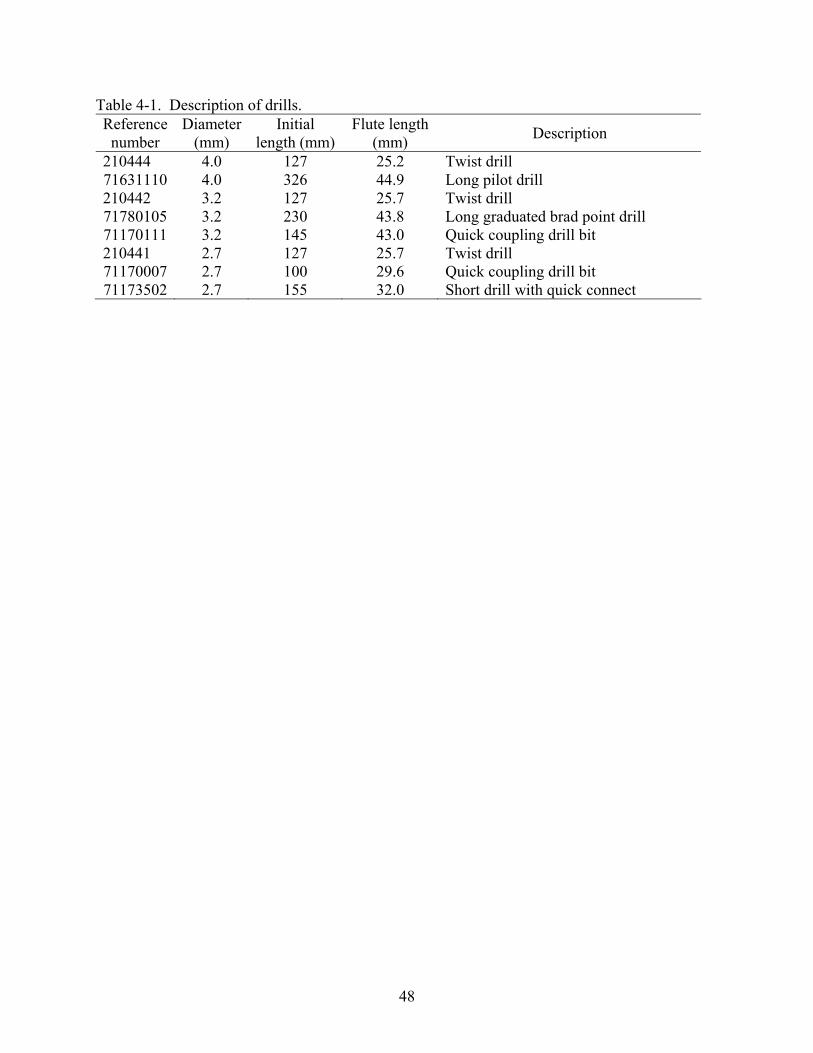
The drills were cut to a uniform length of 72mm using a grinding wheel. The edges were

smoothed and burrs were removed. Details for the drills tested in this study are summarized in

Table 4-1. Figure 4-4 shows the drill geometry and reference number for all the drills tested. To

compare the axial forces during drilling for each drill a 5 axis computer-numerically controlled

milling machine (Mikron UCP 600 Vario) was used. A Kistler 9257B three component

dynamometer was used to measure the axial force. The axial force signals were amplified using a

Kistler Type 5010 charge amplifier and digitally recorded (83,333 sampling frequency) to obtain

the force versus time data. A K type thermocouple was used for drilling temperature

measurement.

Experimental Procedure

The procedure for experiments performed using Sawbones and bovine bone material have

been described below.

40

Sawbones Setup

The Sawbones work-piece was bolted to the aluminum fixtures. The fixtures were in turn

bolted to the dynamometer. The holes were drilled a 4 x 4 pattern with 4 mm spacing between

hole centers. The drilling depth was 10mm. Each drill was used to create a single row (4 holes)

on the work piece. A total of 8 holes per drill were drilled to verify the force repeatability. The

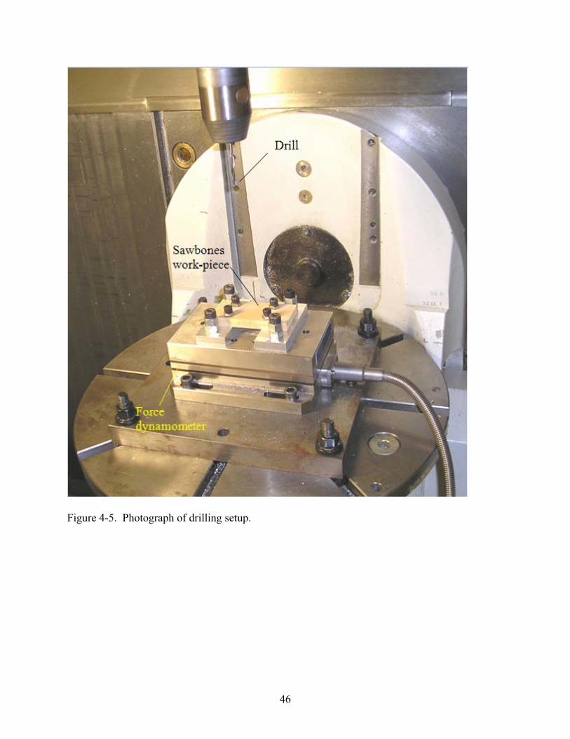
feed per revolution was 0.1 mm/rev (0.004 in/rev) and the spindle speed was 750 rev/min. The

experimental setup for the Sawbone material is shown in the Figure 4-5. The computer

numerically controlled (CNC) drilling sequence for force and temperature measurement was:

• Bolt the sample on to the aluminum fixture (the aluminum fixture was bolted on to the dynamometer).

• Select drill from tool magazine. • Set spindle speed to 750 rpm. • Approach work-piece and drill at constant feed rate (0.1 mm/rev) completely through 10

mm thick test block. • Retract drill. • Immediately (range of 2-4 seconds) measure the temperature at the drill tip using a

contacting K-type thermocouple. • Reposition 4 mm to the right in Figure.4-4. Drill the second hole. • Repeat for a row of four holes. • Select new drill. • Repeat steps 3-8 to drill new row.

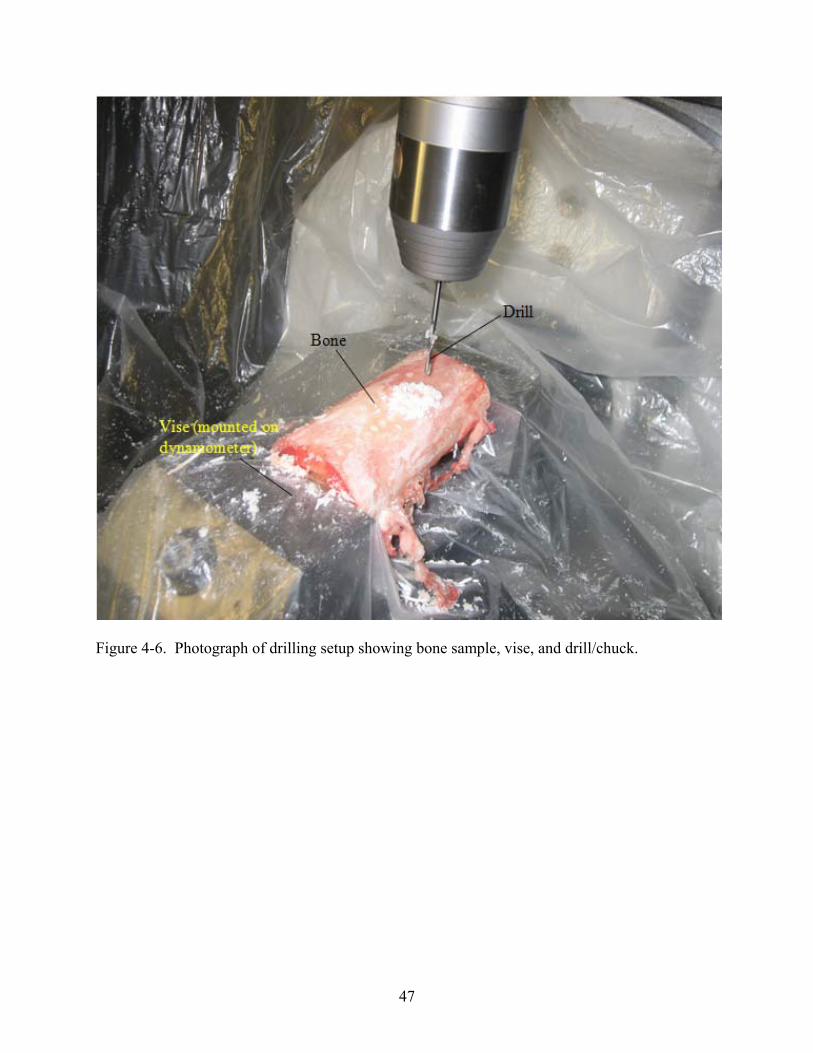
Bovine Bone Setup

A small mounting vise was mounted on the dynamometer. The bovine bone work-piece

was clamped in the vise. The experimental setup for the bovine bone material is shown in the

Figure 4-6. Additionally, in order to improve repeatability in the drilling conditions from one test

to another, a fixed drilling depth in cortical bone only was selected. Therefore, each drill

removed the same depth of cortical material over an identical time period prior to temperature

measurement. It was believed that this was important to enable temperature comparisons

41

between individual drill geometries. The CNC drilling sequence for the force and temperature

measurements was:

• Clamp sample in vise (the vise was mounted on the force dynamometer). • Mill small, localized flat surface on sample using square endmill. • Select drill from tool magazine. • Set spindle speed to 750 rpm. • Approach work-piece and drill at constant feed rate (0.1 mm/rev) through cortical bone to

fixed depth (do not penetrate into cancellous bone). • Retract drill. • Immediately (range of 2-4 seconds) measure the temperature at the drill tip using a

contacting K-type thermocouple. • Reposition 4mm to the top in Figure 4-5. Drill the second hole. • Repeat for a column of 8 holes. • Select new drill. • Repeat steps 4-9 to drill a new column.

42

Figure 4-1. Drill wandering and surface preparation using an end mill. (A) If the drilling surface

is not perpendicular to the drill axis, the drill tends to wander rather than penetrate (picture is exaggerated), (B) Milling a flat surface provides more consistent experimental conditions. Note that the drilling depth was constant and drilling completed in cortical bone only (for temperature measurement consistency).

43

Figure 4-2. Bone work-piece before milling.

44

Figure 4-3. Bone work-piece with its drilling surface flattened by milling.

45

Figure 4-4. Picture of the drills with reference number.

46

Figure 4-5. Photograph of drilling setup.

47

Figure 4-6. Photograph of drilling setup showing bone sample, vise, and drill/chuck.

48

Table 4-1. Description of drills. Reference number

Diameter (mm)

Initial length (mm)

Flute length (mm) Description

210444 4.0 127 25.2 Twist drill 71631110 4.0 326 44.9 Long pilot drill 210442 3.2 127 25.7 Twist drill 71780105 3.2 230 43.8 Long graduated brad point drill 71170111 3.2 145 43.0 Quick coupling drill bit 210441 2.7 127 25.7 Twist drill 71170007 2.7 100 29.6 Quick coupling drill bit 71173502 2.7 155 32.0 Short drill with quick connect

49

CHAPTER 5 RESULT AND DISCUSSION

The results obtained by performing tests on Sawbones material and bovine bone are

presented below.

Force Data

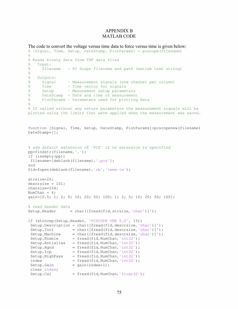
Matlab code is used to convert the voltage versus time data into force versus time data.

Appendix B includes the code used. The force in the X, Y and Z axes are retrieved. The X, Y, Z

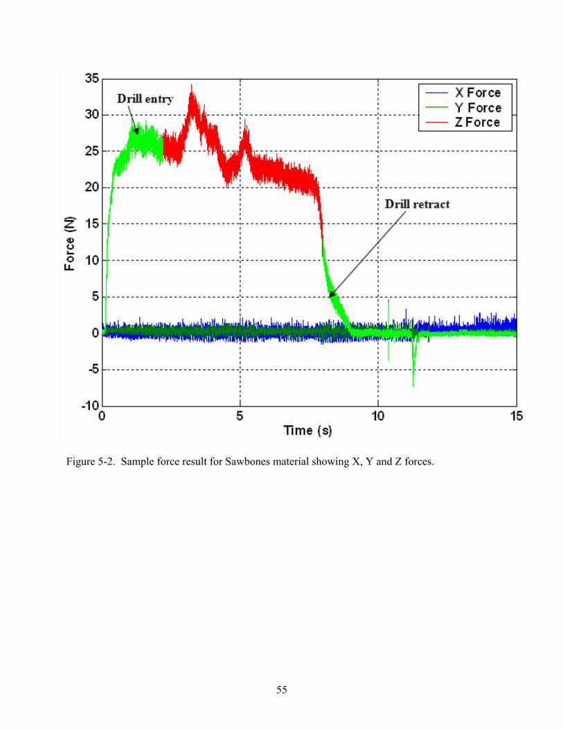
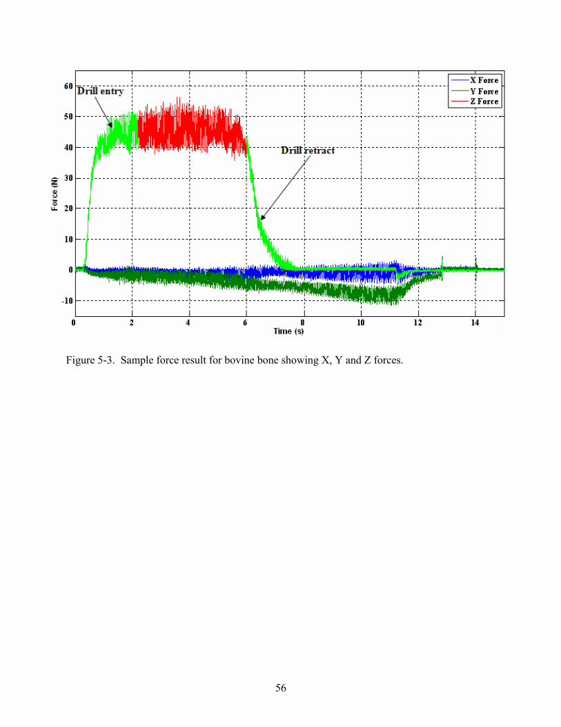
directions are shown in Figure 5-1. Example force record for sawbones and bovine bone material

is shown below in Figure 5-2. and Figure 5-3. The X, Y and Z forces are shown as functions of

drilling time. The entry and exit portions of the hole drilling is included and shown in Figure 5-2.

and Figure 5-3. for each case. This general trend was observed for all eight drills for Sawbones

and bovine bone material.

To compare the force levels between the individual drills, it was necessary to take the drill

diameter into account. Generally, the axial force is considered to be proportional to the hole

(drill) diameter [2]. In other words, if two drills have identical geometries, but one is twice the

diameter of the other, then the axial force would be expected to be twice as high for the larger

diameter drill. To incorporate the influence of diameter, we normalized the peak force to drill

diameter in order to determine the “best” drill from the eights drills considered in this study. The

results for the Sawbones testing are shown in Table 5-1. The table also includes the standard

deviation in the peak force value for 8 repeats per drill to provide an indication of the force

repeatability. The largest percentage for the standard deviation to peak force ratio is 8.4% (for

the long pilot drill with 4.0 mm diameter (71631110), which suggests that the repeatability is

probably sufficient to draw conclusions based on this data. Two sets of tests were performed for

the Sawbones material and bovine bone. For each set, eight holes were drilled using each drill

50

under identical conditions. The experiment was then performed on bovine bone material under

the conditions mentioned in the experimental description for the bovine bone testing. The results

are shown in Table 5-2.

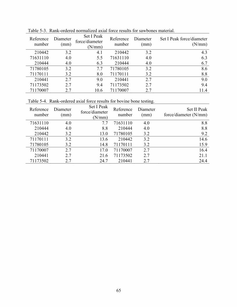
Drills are rank-ordered according to the normalized force value (peak force/diameter). Data

from both the first (I) and second (II) test sets are provided for the Sawbones material and bovine

bone in Table 5-3. and Table 5-4. respectively. In case of Sawbones the normalized peak force

values are identically ordered for sets (I) and (II). For the bovine bone, the position change in

the rank-ordering is never more than two levels between the two independent test sets. It is two

levels for 71780105 (up two relative to the previous data), while it is not more than one level (up

or down) for all the rest. Three of the eight were ranked identically. This is a reasonable result

given the material property variations from one bone sample to another (and variations in

properties from one location to another in the same sample) due to, for example, changes in bone

mineral density.

Tables 5-3 and Table 5-4. both include the drill diameters. It is somewhat suspicious that

the ordering coincides directly with drill diameter (i.e., the largest diameter leads to the smallest

normalized force). With only one exception in case of Sawbones material (drill number 210442)

the ordering is similar to that mentioned above. Recall that the normalized value was obtained by

dividing the peak axial force by the drill diameter (to account for the increase in material

removal); this linear assumption is commonly used in drilling studies with metallic materials

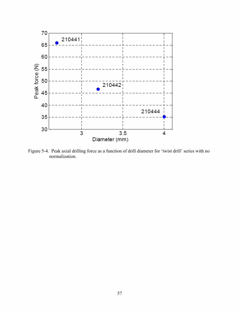
[49]. Although the full details of the edge geometry were not made available, if we assume that

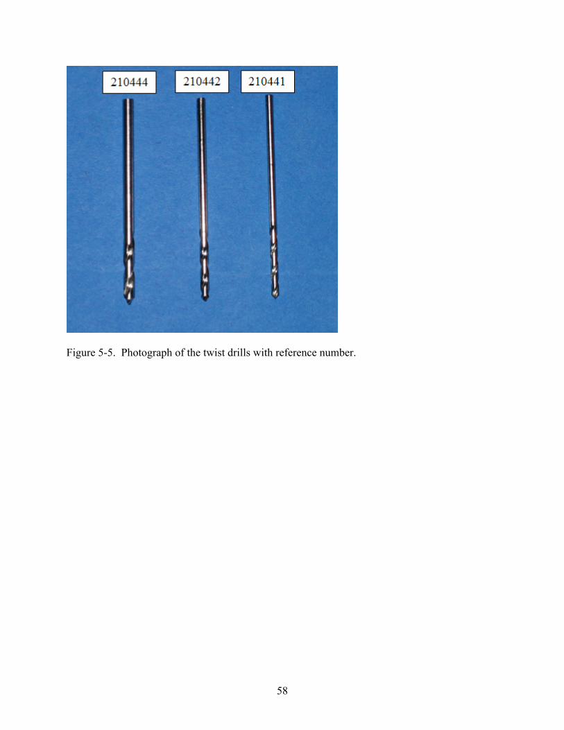
the ‘twist drill’ series – 21044, 210442, and 210441 –only differ by diameter, a comparison of

the peak axial forces can completed. Figure 5-4. shows the peak force as a function of drill

diameter for the ‘twist drills’ in bone. The drill geometry is shown in Figure 5-5. The surprising

51

result is that the force decreases with increasing diameter. We do not have an explanation for this

behavior, but it was consistently exhibited in the bone testing. The validity of the peak force

normalizing procedure could be further explored experimentally by grinding drills with identical

flute geometries, but different diameters. Cutting tests could then be performed to empirically

determine the relationship between force and drill diameter.

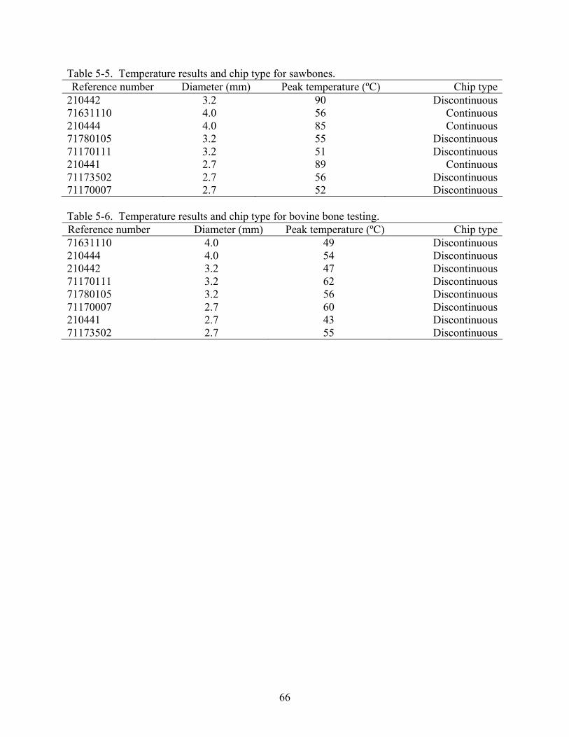
Temperature Data

The average of the peak temperatures recorded at the end of the drilling each hole for each

of the eight drills is shown in Table 5-5. and Table 5-6. The type of chip formed for each drilled

is also included. The peak temperature was recorded during performing the second set of

experiments for the Sawbones material and bovine bone. Although there does not appear to be a

clear trend between temperature and normalized force, if the temperature data is also normalized

by drill diameter (linear relationship again assumed), it is observed that the normalized

temperature is generally lower for the larger drill diameters. It is seen, for example, that the

normalized temperature data gives the same largest to smallest diameter ranking for the ‘twist

drill’ series. However, the trend is not perfectly correlated with force in all cases so that if the

user’s preference is minimum temperature (rather than minimum force), a different drill may be

selected. Finally, it should be noted that the measured drill temperatures were at or above the

temperature range where bone damage can occur (although the damage is believed to depend on

both temperature level and duration of elevated temperature [10]).

Wear Study

It has been reported in the literature that as the drill tends to wear out, the cutting forces

increase [18, 27, 36, 41]. Also a worn drill leads to greater maximum temperature elevation and

longer duration of the temperature elevation [13].

52

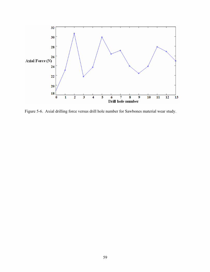
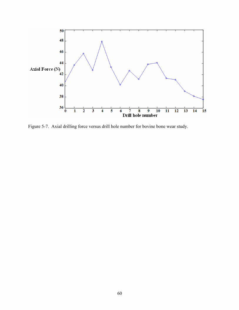
A wear study was performed on the Sawbones and bovine bone material. In this study, 16

holes were made using the same drill. This number was selected since it was representative of

the typical maximum number of holes created by a single drill in a surgical procedure (the drills

are discarded afterwards). The peak axial forces and maximum temperatures were recorded for

each hole. The drill was allowed to cool to room temperature before making the next hole in

order to ensure accurate temperature readings. The plot of peak force and maximum temperature

versus the drill hole number for the two cases have been shown in Figure 5-6. and Figure 5-7.

Chip Formation

The study of chip formation during orthogonal machining of bone has shown that chip

formation occurs by a series of discrete fractures for all cutting orientations. The direction of

fracture propagation is in relation to cutting direction and successive spacing between fractures

during chip formation is found to depend on the orientation of bone specimen during cutting and

depth of cut. It has been reported that the failure tends to be parallel to the predominant direction

of the fibrous matrix of the bones. Values of fracture energy show that it is energetically

favorable for the bone to break in a longitudinal rather than a transverse direction [9]. This

mechanism prevails during drilling as well, although the geometry at the cutting edge for drilling

is much more complex [22].

Microscopic examinations were made of the chips produced by drilling in order to provide

an indication of the chip formation mechanism. At low magnification the chips appear as tight

spirals similar to chips produced while drilling metals. The chips are composed of segments

which are not strongly connected and the shape of the segments indicates that they are separated

from one another by a fracture process, as in case of orthogonal machining. There is also

evidence of deformation caused by the action of the chisel edge. This has been verified in the

literature [22]. Some variation in the chips is brought out about by anisotropy of the bone [9]. A

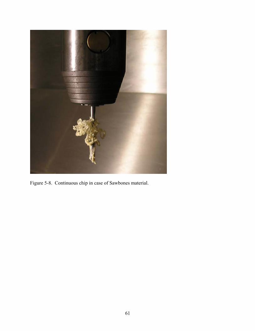
53

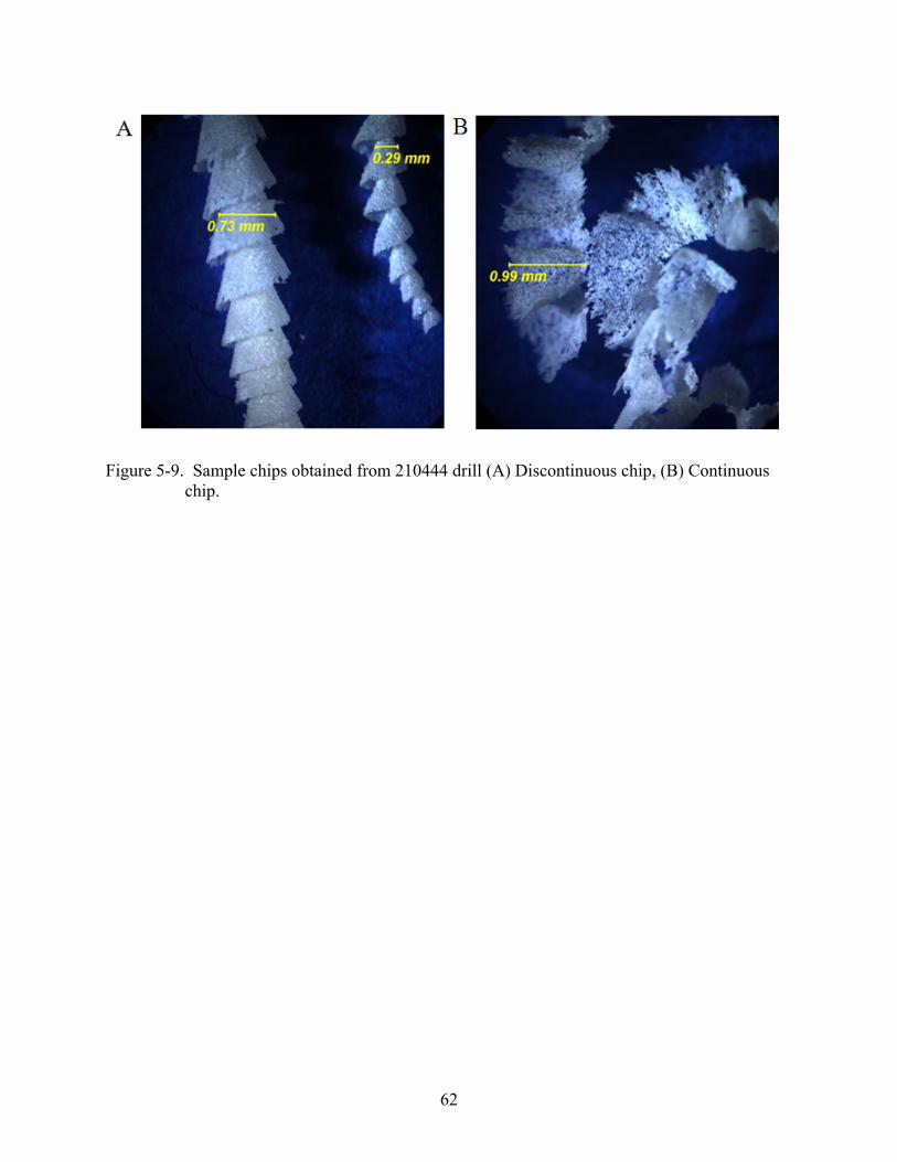
continuous chip formed during the drilling cycle (drill 71631110) is shown by the photograph in

Figure 5-8. Images of chips were collected using a microscope (with CCD camera); examples for

the 210442 (discontinuous) and 210444 (continuous) drills are shown in Figure 5-9.

Hole Description

Images of holes were also collected. A representative example for the Sawbones material

and bovine bone are provided in Figure 5-10. Significant burr formation or edge defects were not

observed on the underside of the drilled holes.

54

Figure 5-1. Drill setup showing the direction of positive X, Y and Z axis.

55

Figure 5-2. Sample force result for Sawbones material showing X, Y and Z forces.

56

Figure 5-3. Sample force result for bovine bone showing X, Y and Z forces.

57

Figure 5-4. Peak axial drilling force as a function of drill diameter for ‘twist drill’ series with no normalization.

58

Figure 5-5. Photograph of the twist drills with reference number.

59

Figure 5-6. Axial drilling force versus drill hole number for Sawbones material wear study.

60

Figure 5-7. Axial drilling force versus drill hole number for bovine bone wear study.

61

Figure 5-8. Continuous chip in case of Sawbones material.

62

Figure 5-9. Sample chips obtained from 210444 drill (A) Discontinuous chip, (B) Continuous chip.

63

Figure 5-10. Images of holes under the microscope. (A) Sawbones, (B) Bovine bone.

64

Table 5-1. Axial force results for sawbones. Set I Set IIReference

number Diameter

(mm) Peak force

(N)

Standard deviation

(N)

Peak force/diameter

(N/mm)

Peak force

(N)

Standard deviation

(N)

Peak force/diameter

(N/mm)71170007 2.7 28.8 1.9 10.6 30.0 0.6 11.471631110 4.0 23.1 1.0 5.5 25.1 2.2 6.3210441 2.7 24.3 1.4 9.0 24.3 0.1 9.0210442 3.2 13.2 0.9 4.1 13.8 0.5 4.371170111 3.2 25.6 1.8 8.0 28.3 2.4 8.8210444 4.0 25.3 1.9 6.3 26.6 0.4 6.771780105 3.2 29.0 1.9 7.7 27.5 0.7 8.671173502 2.7 25.4 1.9 9.4 25.5 0.8 9.4 Table 5-2. Axial force results for bovine bone testing.

Set I Set IIReference number

Diameter (mm) Peak

force (N)

Standard deviation

(N)

Peak force/diameter

(N/mm)

Peak force

(N)

Standard deviation

(N)

Peak force/diameter

(N/mm)71170007 2.7 46.1 0.5 17.0 44.4 4.1 16.471631110 4.0 30.8 3.8 7.7 35.1 0.8 8.8210441 2.7 58.3 9.1 21.6 65.9 2.5 21.1210442 3.2 41.76 3.8 13.0 46.7 0.3 9.271170111 3.2 43.4 2.8 13.6 50.9 2.2 14.6210444 4.0 35.1 2.5 8.8 35.0 0.6 8.871780105 3.2 47.3 8.6 14.8 29.4 2.1 15.971173502 2.7 66.8 1.1 24.7 57.0 1.6 24.4

65

Table 5-3. Rank-ordered normalized axial force results for sawbones material.

Reference number

Diameter (mm)

Set I Peak force/diameter

(N/mm)

Reference number

Diameter (mm)

Set I Peak force/diameter (N/mm)

210442 3.2 4.1 210442 3.2 4.371631110 4.0 5.5 71631110 4.0 6.3

210444 4.0 6.3 210444 4.0 6.771780105 3.2 7.7 71780105 3.2 8.671170111 3.2 8.0 71170111 3.2 8.8

210441 2.7 9.0 210441 2.7 9.071173502 2.7 9.4 71173502 2.7 9.471170007 2.7 10.6 71170007 2.7 11.4

Table 5-4. Rank-ordered axial force results for bovine bone testing.

Reference number

Diameter (mm)

Set I Peak force/diameter

(N/mm)

Reference number

Diameter (mm)

Set II Peak force/diameter (N/mm)

71631110 4.0 7.7 71631110 4.0 8.8210444 4.0 8.8 210444 4.0 8.8210442 3.2 13.0 71780105 3.2 9.2

71170111 3.2 13.6 210442 3.2 14.671780105 3.2 14.8 71170111 3.2 15.971170007 2.7 17.0 71170007 2.7 16.4

210441 2.7 21.6 71173502 2.7 21.171173502 2.7 24.7 210441 2.7 24.4

66

Table 5-5. Temperature results and chip type for sawbones. Reference number Diameter (mm) Peak temperature (ºC) Chip type

210442 3.2 90 Discontinuous71631110 4.0 56 Continuous210444 4.0 85 Continuous71780105 3.2 55 Discontinuous71170111 3.2 51 Discontinuous210441 2.7 89 Continuous71173502 2.7 56 Discontinuous71170007 2.7 52 Discontinuous Table 5-6. Temperature results and chip type for bovine bone testing. Reference number Diameter (mm) Peak temperature (ºC) Chip type71631110 4.0 49 Discontinuous210444 4.0 54 Discontinuous210442 3.2 47 Discontinuous71170111 3.2 62 Discontinuous71780105 3.2 56 Discontinuous71170007 2.7 60 Discontinuous210441 2.7 43 Discontinuous71173502 2.7 55 Discontinuous

67

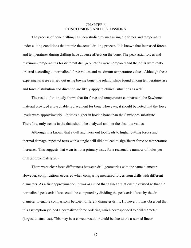
CHAPTER 6 CONCLUSIONS AND DISCUSSIONS

The process of bone drilling has been studied by measuring the forces and temperature

under cutting conditions that mimic the actual drilling process. It is known that increased forces

and temperatures during drilling have adverse affects on the bone. The peak axial forces and

maximum temperatures for different drill geometries were compared and the drills were rank-

ordered according to normalized force values and maximum temperature values. Although these

experiments were carried out using bovine bone, the relationships found among temperature rise

and force distribution and direction are likely apply to clinical situations as well.

The result of this study shows that for force and temperature comparison, the Sawbones

material provided a reasonable replacement for bone. However, it should be noted that the force

levels were approximately 1.9 times higher in bovine bone than the Sawbones substitute.

Therefore, only trends in the data should be analyzed and not the absolute values.

Although it is known that a dull and worn out tool leads to higher cutting forces and

thermal damage, repeated tests with a single drill did not lead to significant force or temperature

increases. This suggests that wear is not a primary issue for a reasonable number of holes per

drill (approximately 20).

There were clear force differences between drill geometries with the same diameter.

However, complications occurred when comparing measured forces from drills with different

diameters. As a first approximation, it was assumed that a linear relationship existed so that the

normalized peak axial force could be computed by dividing the peak axial force by the drill

diameter to enable comparisons between different diameter drills. However, it was observed that

this assumption yielded a normalized force ordering which corresponded to drill diameter

(largest to smallest). This may be a correct result or could be due to the assumed linear

68

relationship between diameter and axial force. Further testing will be required. It was seen that

the force per unit diameter was inversely proportional to drill diameter.

Drill point temperature measurements showed levels which could lead to bone damage for

the selected cutting conditions. The findings suggest that drilling parameters should be changed

to reduce the temperature from the point of view of thermal damage. Normalizing the maximum

temperature to drill diameter provided an ordering sequence with a trend similar to force data

(larger drills generally gave a lower normalized temperature), but did not give exact correlation.

Therefore, a drill which exhibited the lowest force may not yield the lowest temperature. The

factors associated with higher forces, temperature and other clinical consideration appear to

dictate the choice of drill/reamers for a particular cutting operation.

The current study did have some limitations:

• Though the bone is thawed to room temperature, there is a difference between actual body temperature and room temperature. Also vivo blood flow helps in reducing the cortical bone temperature. This does not have a significant effect as the flow rate is small and coagulation of these small vessels occurs due to heating.

• There are variations along the bone due to difference in properties in the bone sample [3, 4].

• In vitro there is less specific heat than vivo bone because of less water content; hence, less energy is required to produce the same temperature increase.

• A five axis CNC machine was used instead of an orthopedic surgical drill. Drill speeds close to actual surgical speeds were used with constant axial force, but the axial force varies in actual practice due to variation in pressure applied by surgeon [13]. It has been reported that for electrically powered drills, the speeds depend on the applied force and the differences are as high as 50% between free running speed (manufacturer's listed speed) and the speed under load [6].

69

CHAPTER 7 FUTURE WORK

Force appears to provide a reasonable metric to rate drill performance. In future work a

mechanistic model of drilling force based on the geometry which quantifies the effect of changes

in drill geometry on force should be developed. Given that temperature is also a critical issue in

drilling success, the mechanistic drilling model could be augmented to perform heat transfer

calculations and estimate drilling temperature.

Optimization of drill geometry consists of reducing cutting effort to a minimum level, as

well as limiting the rise in bone temperature and effective removal of bone chips. Factors such as

time taken for drilling the bone cortex, elimination of walking on curved bone, and required

dimensional tolerance are also instrumental in determining the geometry of the drill [6].

Geometrical parameters such as rake angle, point angle, helix angle, flute geometry, and chisel

edge can be varied to optimize drill design. Drill geometry modeling requires knowledge of the

material being used in order to determine the physical characteristic of the bit. It is also

necessary to account for inherent variation in bone material properties from one subject to the

next and from one location to another in a single bone [12]. Because the mechanistic/thermal

model will require: a) calibration data for force; and b) heat transfer characteristics of the bone,

the predictions should be made over the anticipated range in the simulation input values. This

will enable the user to see the influence of their variation and verify that the effects of drill

geometry changes are not obscured by the effects of material property changes. Another area to

be explored would be to use nonconventional machining processes such as laser drilling.

Appendix A is included which describes the initial results from laser drilling in bone.

70

APPENDIX A LASER BONE ABLATION

This section holds the results of the laser drilling test. In this case, rather than mechanically

removing the bone material, it was ablated by the laser (photon) energy.

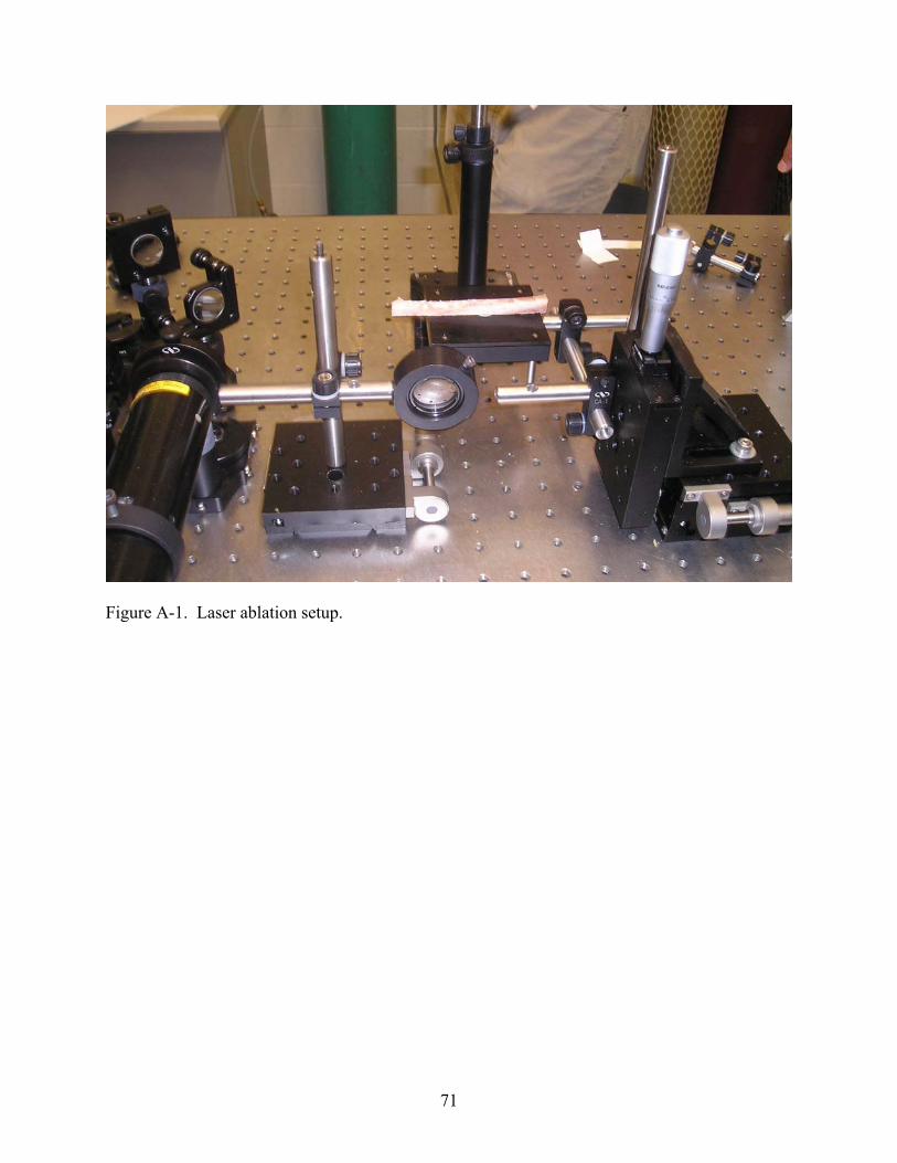
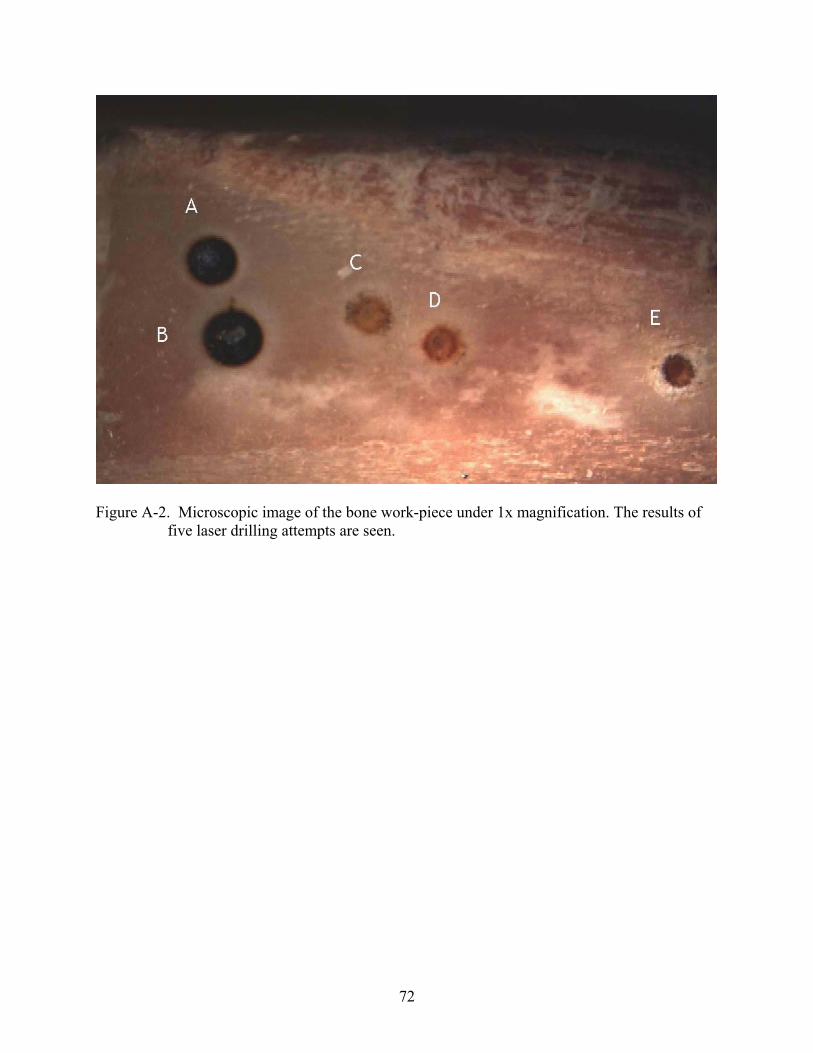
It was performed using a 193 nm wavelength ArF excimer laser. Figure A-1 shows the

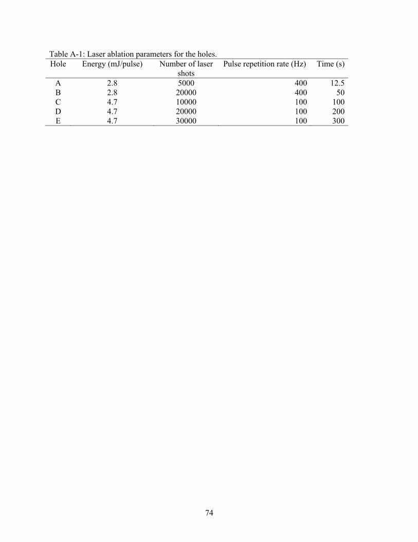
laser ablation setup. Figure A-2 shows five hole making attempts in the bovine bone using the

parameters identified in Table A-1. It appeared that there was a laser energy threshold which

needed to be exceeded to remove materials. Attempts A and B did not lead to holes; instead the

bone was simply charred. With increased energy, however, holes were created for tests C-E. The

increased number of laser pulses from test to test led to progressively deeper holes. It is

estimated that the E condition yielded a 1 mm diameter hole with a depth of approximately 1

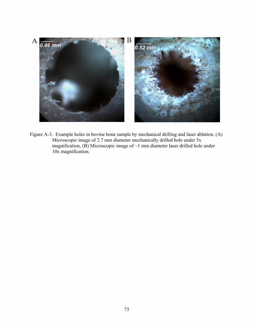
mm. Microscopic images of a mechanically drilled hole and the laser drilled hole E are provided

in Figure A-3. for comparison purposes (same bone work-piece, different locations).

71

Figure A-1. Laser ablation setup.

72

Figure A-2. Microscopic image of the bone work-piece under 1x magnification. The results of five laser drilling attempts are seen.

73

Figure A-3. Example holes in bovine bone sample by mechanical drilling and laser ablation. (A)

Microscopic image of 2.7 mm diameter mechanically drilled hole under 5x magnification, (B) Microscopic image of ~1 mm diameter laser drilled hole under 10x magnification.

74

Table A-1: Laser ablation parameters for the holes. Hole Energy (mJ/pulse) Number of laser

shots Pulse repetition rate (Hz) Time (s)

A 2.8 5000 400 12.5B 2.8 20000 400 50C 4.7 10000 100 100D 4.7 20000 100 200E 4.7 30000 100 300

75

APPENDIX B MATLAB CODE

The code to convert the voltage versus time data to force versus time is given below: % [Signal, Time, Setup, DateStamp, PlotParams] = pcscope(filename) % % Reads binary data from TXF data files % Input: % filename - PC Scope filename and path (matlab text string) % % Outputs: % Signal - Measurement signals (one channel per column) % Time - Time vector for signals % Setup - Mesurement setup parameters % DateStamp - Date and time of measurement % PlotParams - Parameters used for plotting data % % If called without any return parameters the measurement signals will be plotted using the limits that were applied when the measurement was saved. function [Signal, Time, Setup, DateStamp, PlotParams]=pcscopenew(filename) DateStamp=[]; % add default extension of 'PCS' if no extension is specified pp=findstr(filename,'.'); if (isempty(pp)) filename=[deblank(filename),'.pcs']; end fid=fopen(deblank(filename),'rb','ieee-le'); strsize=26; descrsize = 101; charsize=104; NumChan = 4; gain=[0.5; 1; 2; 5; 10; 20; 50; 100; 1; 2; 5; 10; 20; 50; 100]; % read header data Setup.Header = char([fread(fid,strsize,'char')]'); if (strncmp(Setup.Header, 'PCSCOPE VER 5.0', 15)) Setup.Description = char([fread(fid,descrsize,'char')]'); Setup.Tool = char([fread(fid,descrsize,'char')]'); Setup.Machine = char([fread(fid,descrsize,'char')]'); Setup.Enable = fread(fid,NumChan,'int32'); Setup.Antialias = fread(fid,NumChan,'int32'); Setup.Agnd = fread(fid,NumChan,'int32'); Setup.Icp = fread(fid,NumChan,'int32'); Setup.HighPass = fread(fid,NumChan,'int32'); index = fread(fid,NumChan,'int32'); Setup.Gain = gain(index+1); clear index; Setup.Cal = fread(fid,NumChan,'float32');

76

Setup.Unit(1,:) = char([fread(fid,strsize,'char')]'); Setup.Unit(2,:) = char([fread(fid,strsize,'char')]); Setup.Unit(3,:) = char([fread(fid,strsize,'char')]); Setup.Unit(4,:) = char([fread(fid,strsize,'char')]); Setup.Name(1,:) = char([fread(fid,strsize,'char')]'); Setup.Name(2,:) = char([fread(fid,strsize,'char')]); Setup.Name(3,:) = char([fread(fid,strsize,'char')]); Setup.Name(4,:) = char([fread(fid,strsize,'char')]); Setup.TrigMethod = fread(fid,1,'int32'); Setup.TrigLevel = fread(fid,1,'float32'); Setup.TrigSlope = fread(fid,1,'int32'); Setup.TrigMode = fread(fid,1,'int32'); Setup.TrigSource = fread(fid,1,'int32'); Setup.TrigTimer = fread(fid,1,'float32'); Setup.TrigTimerUnits = fread(fid,1,'float32'); Setup.SampFreq = fread(fid,1,'float32'); Setup.Decimate = fread(fid,1,'int32'); Setup.SampTime = fread(fid,1,'float32'); Setup.PretrigTime = fread(fid,1,'float32'); Setup.Window = fread(fid,NumChan,'int32'); Setup.Integration = fread(fid,NumChan,'int32'); Setup.Autoscale(1).min = fread(fid, 1, 'float64'); Setup.Autoscale(1).max = fread(fid, 1, 'float64'); Setup.Autoscale(2).min = fread(fid, 1, 'float64'); Setup.Autoscale(2).max = fread(fid, 1, 'float64'); Setup.Autoscale(3).min = fread(fid, 1, 'float64'); Setup.Autoscale(3).max = fread(fid, 1, 'float64'); Setup.Autoscale(4).min = fread(fid, 1, 'float64'); Setup.Autoscale(4).max = fread(fid, 1, 'float64'); Setup.FftSize = fread(fid,1,'int32'); Setup.Harmonics = fread(fid,1,'int32'); Setup.DataLogEnable = fread(fid,1,'int32'); Setup.DataLogLogFilename = char([fread(fid,512,'char')]'); Setup.DataLogStartLogNum = fread(fid,1,'int32'); Setup.DataLogLogDurationUnits = fread(fid,1,'int32'); Setup.DataLogLogDurationfval = fread(fid,1,'float32'); for i=1:10 Setup.Filtertype(i) = fread(fid,1,'int32'); Setup.Filterorder(i) = fread(fid,1,'int32'); Setup.Filterfreq(i) = fread(fid,1,'float32'); Setup.Filterband(i) = fread(fid,1,'float32'); Setup.Filterharm(i) = fread(fid,1,'int32'); Setup.Filterchan(i) = fread(fid,1,'int32'); end DateStamp.Year = fread(fid,1,'int16'); DateStamp.Month = fread(fid,1,'int16');

77

DateStamp.Dayofweek = fread(fid,1,'int16'); DateStamp.Day = fread(fid,1,'int16'); DateStamp.Hour = fread(fid,1,'int16'); DateStamp.minute = fread(fid,1,'int16'); DateStamp.Second = fread(fid,1,'int16'); DateStamp.Millisecond = fread(fid,1,'int16'); for i=1:4 PlotParams.EnableAutoscale(i) = fread(fid,1,'int32'); PlotParams.Xmin(i)= fread(fid,1,'float64'); PlotParams.Xmax(i)= fread(fid,1,'float64'); PlotParams.Xdiv(i)= fread(fid,1,'int32'); PlotParams.Ymin(i)= fread(fid,1,'float64'); PlotParams.Ymax(i)= fread(fid,1,'float64'); PlotParams.Ydiv(i)= fread(fid,1,'int32'); PlotParams.CursorIndex(i) = fread(fid,1,'int32'); end elseif (strncmp(Setup.Header, 'PCSCOPE VER 4.0', 15)) Setup.Description = char([fread(fid,descrsize,'char')]'); Setup.Tool = char([fread(fid,descrsize,'char')]'); Setup.Machine = char([fread(fid,descrsize,'char')]'); Setup.Enable = fread(fid,NumChan,'int32'); Setup.Antialias = fread(fid,NumChan,'int32'); Setup.Agnd = fread(fid,NumChan,'int32'); Setup.Icp = fread(fid,NumChan,'int32'); Setup.HighPass = fread(fid,NumChan,'int32'); index = fread(fid,NumChan,'int32'); Setup.Gain = gain(index+1); clear index; Setup.Cal = fread(fid,NumChan,'float32'); Setup.Unit(1,:) = char([fread(fid,strsize,'char')]'); Setup.Unit(2,:) = char([fread(fid,strsize,'char')]); Setup.Unit(3,:) = char([fread(fid,strsize,'char')]); Setup.Unit(4,:) = char([fread(fid,strsize,'char')]); Setup.Name(1,:) = char([fread(fid,strsize,'char')]'); Setup.Name(2,:) = char([fread(fid,strsize,'char')]); Setup.Name(3,:) = char([fread(fid,strsize,'char')]); Setup.Name(4,:) = char([fread(fid,strsize,'char')]); Setup.TrigMethod = fread(fid,1,'int32'); Setup.TrigLevel = fread(fid,1,'float32'); Setup.TrigSlope = fread(fid,1,'int32'); Setup.TrigMode = fread(fid,1,'int32'); Setup.TrigSource = fread(fid,1,'int32'); Setup.SampFreq = fread(fid,1,'float32'); Setup.SampTime = fread(fid,1,'float32'); Setup.PretrigTime = fread(fid,1,'float32'); Setup.Window = fread(fid,NumChan,'int32'); Setup.Integration = fread(fid,NumChan,'int32');

78

Setup.Autoscale(1).min = fread(fid, 1, 'float64'); Setup.Autoscale(1).max = fread(fid, 1, 'float64'); Setup.Autoscale(2).min = fread(fid, 1, 'float64'); Setup.Autoscale(2).max = fread(fid, 1, 'float64'); Setup.Autoscale(3).min = fread(fid, 1, 'float64'); Setup.Autoscale(3).max = fread(fid, 1, 'float64'); Setup.Autoscale(4).min = fread(fid, 1, 'float64'); Setup.Autoscale(4).max = fread(fid, 1, 'float64'); Setup.FftSize = fread(fid,1,'int32'); Setup.Harmonics = fread(fid,1,'int32'); DateStamp.Year = fread(fid,1,'int16'); DateStamp.Month = fread(fid,1,'int16'); DateStamp.Dayofweek = fread(fid,1,'int16'); DateStamp.Day = fread(fid,1,'int16'); DateStamp.Hour = fread(fid,1,'int16'); DateStamp.minute = fread(fid,1,'int16'); DateStamp.Second = fread(fid,1,'int16'); DateStamp.Millisecond = fread(fid,1,'int16'); PlotParams.Xmin(1)= fread(fid,1,'float64'); PlotParams.Xmax(1)= fread(fid,1,'float64'); PlotParams.Xdiv(1)= fread(fid,1,'int32'); PlotParams.Ymin(1)= fread(fid,1,'float64'); PlotParams.Ymax(1)= fread(fid,1,'float64'); PlotParams.Ydiv(1)= fread(fid,1,'int32'); PlotParams.Xmin(2)= fread(fid,1,'float64'); PlotParams.Xmax(2)= fread(fid,1,'float64'); PlotParams.Xdiv(2)= fread(fid,1,'int32'); PlotParams.Ymin(2)= fread(fid,1,'float64'); PlotParams.Ymax(2)= fread(fid,1,'float64'); PlotParams.Ydiv(2)= fread(fid,1,'int32'); elseif (strncmp(Setup.Header, 'PCSCOPE VER 3.0', 15) | strncmp(Setup.Header, 'PCSCOPE VER 3.1', 15)) Setup.Description = char([fread(fid,descrsize,'char')]'); Setup.Tool = char([fread(fid,descrsize,'char')]'); Setup.Machine = char([fread(fid,descrsize,'char')]'); Setup.Enable = fread(fid,NumChan,'int32'); Setup.Antialias = fread(fid,NumChan,'int32'); index = fread(fid,NumChan,'int32'); Setup.Gain = gain(index+1); clear index; Setup.Cal = fread(fid,NumChan,'float32'); Setup.Unit(1,:) = char([fread(fid,strsize,'char')]'); Setup.Unit(2,:) = char([fread(fid,strsize,'char')]); Setup.Unit(3,:) = char([fread(fid,strsize,'char')]); Setup.Unit(4,:) = char([fread(fid,strsize,'char')]); Setup.Name(1,:) = char([fread(fid,strsize,'char')]'); Setup.Name(2,:) = char([fread(fid,strsize,'char')]); Setup.Name(3,:) = char([fread(fid,strsize,'char')]); Setup.Name(4,:) = char([fread(fid,strsize,'char')]);

79

Setup.TrigMethod = fread(fid,1,'int32'); Setup.TrigLevel = fread(fid,1,'float32'); Setup.TrigSlope = fread(fid,1,'int32'); Setup.TrigMode = fread(fid,1,'int32'); Setup.SampFreq = fread(fid,1,'float32'); Setup.SampTime = fread(fid,1,'float32'); Setup.PretrigTime = fread(fid,1,'float32'); Setup.Window = fread(fid,NumChan,'int32'); Setup.Integration = fread(fid,NumChan,'int32'); Setup.Autoscale(1).min = fread(fid, 1, 'float64'); Setup.Autoscale(1).max = fread(fid, 1, 'float64'); Setup.Autoscale(2).min = fread(fid, 1, 'float64'); Setup.Autoscale(2).max = fread(fid, 1, 'float64'); Setup.Autoscale(3).min = fread(fid, 1, 'float64'); Setup.Autoscale(3).max = fread(fid, 1, 'float64'); Setup.Autoscale(4).min = fread(fid, 1, 'float64'); Setup.Autoscale(4).max = fread(fid, 1, 'float64'); Setup.FftSize = fread(fid,1,'int32'); Setup.Harmonics = fread(fid,1,'int32'); DateStamp.Year = fread(fid,1,'int16'); DateStamp.Month = fread(fid,1,'int16'); DateStamp.Dayofweek = fread(fid,1,'int16'); DateStamp.Day = fread(fid,1,'int16'); DateStamp.Hour = fread(fid,1,'int16'); DateStamp.minute = fread(fid,1,'int16'); DateStamp.Second = fread(fid,1,'int16'); DateStamp.Millisecond = fread(fid,1,'int16'); PlotParams.Xmin(1)= fread(fid,1,'float64'); PlotParams.Xmax(1)= fread(fid,1,'float64'); PlotParams.Xdiv(1)= fread(fid,1,'int32'); PlotParams.Ymin(1)= fread(fid,1,'float64'); PlotParams.Ymax(1)= fread(fid,1,'float64'); PlotParams.Ydiv(1)= fread(fid,1,'int32'); PlotParams.Xmin(2)= fread(fid,1,'float64'); PlotParams.Xmax(2)= fread(fid,1,'float64'); PlotParams.Xdiv(2)= fread(fid,1,'int32'); PlotParams.Ymin(2)= fread(fid,1,'float64'); PlotParams.Ymax(2)= fread(fid,1,'float64'); PlotParams.Ydiv(2)= fread(fid,1,'int32'); elseif (strncmp(Setup.Header, 'PCSCOPE VER 2.0', 15)) Setup.Description = char([fread(fid,descrsize,'char')]'); Setup.Tool = char([fread(fid,descrsize,'char')]'); Setup.Machine = char([fread(fid,descrsize,'char')]'); Setup.Enable = fread(fid,NumChan,'int32'); Setup.Antialias = fread(fid,NumChan,'int32'); index = fread(fid,NumChan,'int32'); Setup.Gain = gain(index+1); clear index;

80

Setup.Cal = fread(fid,NumChan,'float32'); Setup.Unit(1,:) = char([fread(fid,strsize,'char')]'); Setup.Unit(2,:) = char([fread(fid,strsize,'char')]); Setup.Unit(3,:) = char([fread(fid,strsize,'char')]); Setup.Unit(4,:) = char([fread(fid,strsize,'char')]); Setup.TrigMethod = fread(fid,1,'int32'); Setup.TrigLevel = fread(fid,1,'float32'); Setup.TrigSlope = fread(fid,1,'int32'); Setup.TrigMode = fread(fid,1,'int32'); Setup.SampFreq = fread(fid,1,'float32'); Setup.SampTime = fread(fid,1,'float32'); Setup.PretrigTime = fread(fid,1,'float32'); DateStamp.Year = fread(fid,1,'int16'); DateStamp.Month = fread(fid,1,'int16'); DateStamp.Dayofweek = fread(fid,1,'int16'); DateStamp.Day = fread(fid,1,'int16'); DateStamp.Hour = fread(fid,1,'int16'); DateStamp.minute = fread(fid,1,'int16'); DateStamp.Second = fread(fid,1,'int16'); DateStamp.Millisecond = fread(fid,1,'int16'); PlotParams.Xmin(1)= fread(fid,1,'float64'); PlotParams.Xmax(1)= fread(fid,1,'float64'); PlotParams.Xdiv(1)= fread(fid,1,'int32'); PlotParams.Ymin(1)= fread(fid,1,'float64'); PlotParams.Ymax(1)= fread(fid,1,'float64'); PlotParams.Ydiv(1)= fread(fid,1,'int32'); PlotParams.Xmin(2)= fread(fid,1,'float64'); PlotParams.Xmax(2)= fread(fid,1,'float64'); PlotParams.Xdiv(2)= fread(fid,1,'int32'); PlotParams.Ymin(2)= fread(fid,1,'float64'); PlotParams.Ymax(2)= fread(fid,1,'float64'); PlotParams.Ydiv(2)= fread(fid,1,'int32'); elseif (strncmp(Setup.Header, 'PCSCOPE VER 1.0', 15)) Setup.Description = char([fread(fid,descrsize,'char')]'); Setup.Enable = fread(fid,NumChan,'int32'); Setup.Antialias = fread(fid,NumChan,'int32'); index = fread(fid,NumChan,'int32'); Setup.Gain = gain(index+1); clear index; Setup.Cal = fread(fid,NumChan,'float32'); Setup.Unit(1,:) = char([fread(fid,strsize,'char')]'); Setup.Unit(2,:) = char([fread(fid,strsize,'char')]); Setup.Unit(3,:) = char([fread(fid,strsize,'char')]); Setup.Unit(4,:) = char([fread(fid,strsize,'char')]); Setup.TrigMethod = fread(fid,1,'int32'); Setup.TrigLevel = fread(fid,1,'float32'); Setup.TrigSlope = fread(fid,1,'int32'); Setup.TrigMode = fread(fid,1,'int32');

81

Setup.SampFreq = fread(fid,1,'float32'); Setup.SampTime = fread(fid,1,'float32'); Setup.PretrigTime = fread(fid,1,'float32'); end if (strncmp(Setup.Header, 'PCSCOPE VER 5.0', 15)) for i=1:4 ShowChan(i) = fread(fid,1,'uint32'); end iFftStart(1)=fread(fid,1,'int32'); iFftStart(2)=fread(fid,1,'int32'); iFftWindow(1)=fread(fid,1,'int32'); iFftWindow(2)=fread(fid,1,'int32'); end % TimLen is set to NumSampPerChan and set active channels and number of channels NumSampPerChan=fread(fid,1,'uint32')-1; ActiveChans = find(Setup.Enable == 1); NumChanSamp=length(ActiveChans); Signal = [reshape(fread(fid,NumChanSamp*NumSampPerChan,'int16'), NumSampPerChan,NumChanSamp)]'; Signal = Signal' * diag((Setup.Cal(ActiveChans))./(Setup.Gain(ActiveChans))) / 409.6; Time = [0:NumSampPerChan-1]'/Setup.SampFreq; fclose(fid); % if there are no return parameters, plot the data on screen with the same limits % used when the measurement was saved if nargout == 0 hax = gca; % change plot colors MatlabColors = get(hax, 'ColorOrder'); PCScopeColors = [0,0,255;255,0,0;0,180,80;255,0,255]/255; Samp = 1; for i=1:4 if Setup.Enable(i) ~= 0 MatlabColors(Samp,:) = PCScopeColors(i,:); Samp = Samp + 1; end end set(hax,'ColorOrder',MatlabColors); % plot all channels on one plot plot(Time, Signal) grid hxl=xlabel('Time, s'); htl=title(Setup.Description);

82

% set font size set([hxl,htl,hax],'FontSize',12); zoom on % clear return parameters to prevent echoing to the terminal clear Signal Time Setup DateStamp PlotParams end

83

LIST OF REFERENCES

1. Udiljak, Ciglar, Skoric, 2007, “Investigation into bone drilling and thermal bone necrosis,” Advances in production engineering and management, 2(3), pp 103-112

2. Egger el, Histand MB, Blass CE, Powers BE, 1986, “Effect of fixation pin insertion on the bone-pin interface,” Veterinary surgery, 15 (3), pp 246-252

3. Hillery M.T., Shuaib I, 1999, “Temperature effects in the drilling of human and bovine bone,” Journal of Materials Processing Technology, 92-93, pp 302-308

4. Hobkirk, J.A. and Rusiniak, K.J., 1977, “Investigation of Variable Factors in Drilling,” Bone Oral Surgery, 35, pp 968-973

5. Wiggins Kl, Malkin S, 1976, “Drilling of bone,” Journal of biomechanics, 9 (9), pp 553

6. J -Y Giraud, S Villemin, R Darmana, J -Ph Cahuzac, A Autefage and J -P Morucci,

7. 1991, “Bone cutting,” Clin. Phys. Physiol. Meas, 12(1), pp 1-19

8. Mustafa , abouzgia, david f. James, 1995, “Measurements of shaft speed while drilling through bone,” International journal of oral & maxillofacial surgery, pp 1315- 1316

9. Larry s. Matthews and Carl Hirsch, 1972, “Temperatures measured in human cortical bone when drilling,” Journal of bone and joint surgery, 54, pp 297-308

10. Kent N. Bachus, Matthew T. Rondina , Douglas T. Hutchinson, “The effects of drilling force on cortical temperatures and their duration : an in vitro study,”

11. Sean R. H. Davidson and David F. James, 2003, “Drilling in Bone: Modeling Heat Generation and Temperature Distribution,”, Journal of Biomechanical Engineering, 125(3), pp 305-314

12. Natali C, Ingle P, Dowell J, 1996, “Orthopaedic bone drills-can they be improved? Temperature changes near the drilling face,” Journal of Bone and Joint Surgery ( Br), 78(3), pp 357-62

13. Eriksson A, Albrektsson T, Grane B, Mcqueen D, 1982, “Thermal-Injury To Bone - A Vital-Microscopic Description Of Heat-Effects,” International Journal of Oral Surgery, 11 (2), pp 115-121

14. Allotta B, Belmonte F, Bosio L, Dario P, 1996, “Study on a mechatronic tool for drilling in the osteosynthesis of long bones tool-bone interaction, modeling and experiments,” Mechatronics(Oxford), 6(4), pp 447-459

84

15. Oscar G. Riquelme García, Fausto López Mombiela, Consuelo Jiménez de la Fuente, Margarita Gimeno Aránguez, Dolores Vigil Escribano, Javier Vaquero Martín, 2004, “The Influence of the Size and Condition of the Reamers on Bone Temperature During Intramedullary Reaming,” The Journal of Bone and Joint Surgery (American), 86, pp 994-999

16. Lavelle C, Wedgwood D, 1980, “Effect of internal irrigation on frictional heat generated from bone drilling,” Journal of Oral Surgery,38(7), pp 499-503

17. Abouzgia MB, Symington JM, 1996, “Effect of drill speed on bone temperature,” International Journal of Oral & Maxillofacial Surgery, 25(5), pp 394-9

18. LS Matthews, CA Green and SA Goldstein, 1984, “The thermal effects of skeletal fixation-pin insertion in bone,” Journal of bone and joint surgery, 66, pp 1077-1083

19. , 1997, “Temperature rise during drilling through bone,” The International Journal of Oral & Maxillofacial Implants, 12(3), pp 342-53

20. Eriksson AR, Albrektsson T, Albrektsson B, 1984, “Heat caused by drilling cortical bone - temperature measured invivo in patients and animals,” Acta orthopaedica scandinavica, 55 (6), pp 629-631

21. Sedlin ED, Hirsch C, 1966, “ Factors affecting determination of physical properties of femoral cortical bone,” Acta Orthopaedica Scandinavica, 37 (1), pp 29

22. Influence of strain rate on the mechanical behavior of cortical bone interstitial lamellae at the micrometer scale

23. Cody, D.D.; McCubbrey, D.A., Divine, G.W., Gross, G.J., Goldstein, S.A., 1996, "Predictive Value of Proximal Femoral Bone Densitometry in Determining Local Orthogonal Material Properties," Journal of Biomechanics 29 (6), pp 753-762

24. Wachter N.J.1; Krischak G.D.; Mentzel M.; Sarkar M.R.; Ebinger T.; Kinzl L.; Claes L.; Augat P, 2002, “Correlation of bone mineral density with strength and microstructural parameters of cortical bone in vitro,” Bone, 31(1), pp. 90-95

25. Sherman spatz , “Early reaction in bone following the use of burs rotating at conventional and ultra high speeds”

26. Reingewirtz Y, Szmukler-Moncler S, Senger B., 1997, “Influence of different parameters on bone heating and drilling time in implantology,” Clinical Oral Implants Research, 8(3), pp 189-97

27. Jacob CH, Berry JT, 1976, “A study of the bone machining process-drilling,” Journal of Biomechanics, pp 343-9

28. Jacobs RL, Ray RD, 1972, “ Effect of heat on bone healing - disadvantage in use of power tools,” Archives of surgery, 104 (5), pp 687

85

29. Ohashi H, Therin M, Meunier A, Christel P , 1994, “The Effect Of Drilling Parameters On Bone .1. General Healing Response,” Journal of Materials Science-Materials in Medicine, 5 (4), pp 225-231

30. Allan W, Williams ED, Kerawala CJ, 2005, “Effects of repeated drill use on temperature of bone during preparation for osteosynthesis self-tapping screws,” British Journal of Oral and Maxillofacial Surgery, 43, pp 314-9

31. Ercoli C, Funkenbusch PD, Lee HJ, Moss ME, Graser GN , 2004, “The influence of drill wear on cutting efficiency and heat production during osteotomy preparation for dental implants: A study of drill durability,” International Journal of Oral & Maxillofacial Implants, 19 (3), pp 335-349

32. Lavelle C, Wedgwood D, 1980, “Effect of internal irrigation on frictional heat generated from bone drilling,” Journal of Oral Surgery, 38 (7), pp 499-503

33. Higgins TE (Higgins, Thomas E.), Casey V (Casey, Virginia), Bachus K (Bachus, Kent), 2007, “Cortical heat generation using an irrigating/aspirating single-pass reaming vs conventional stepwise reaming,” Journal of Orthopedic Trauma, 21 (3), pp 192-197

34. Toews AR, Bailey JV, Townsend HGG, Barber SM, 1999, “Effect of feed rate and drill speed on temperatures in equine cortical bone,” American Journal of Veterinary Research, 60 (8), pp 942-944

35. Krause WR, Bradbury DW, Kelly JE, Lunceford EM, “Temperature elevations in orthopedic cutting operations,”

36. Jacobs CH, Pope MH, Berry JT, Hoaglund F, 1974, “A study of the bone machining process-orthogonal cutting,” Journal of Biomechanics, 7(2), pp 131-6

37. Peyton, 1952, “Temperature rise and cutting efficiency of rotating instrument,” NY Sent J, 18, pp 439-450

38. Larry S. Matthews, Carl Hirsch, 1972, “Temperatures measured in human cortical bone when drilling,” The journal of bone and joint surgery (American), 54, pp 297-308

39. Volkov MV, Shepeleva IS, 1974, “Use of ultrasonic instrumentation for transection and uniting of bone tissue in orthopedic surgery,”Reconstruction Surgery and Traumatology, 14, pp 147-152

40. Horton Je, Tarpley Tm, Jacoway Jr, 1981, “Clinical-Applications Of Ultrasonic Instrumentation In The Surgical Removal Of Bone ,” Oral Surgery Oral Medicine Oral Pathology Oral Radiology And Endodontics, 51 (3), pp 236-242

41. Gruber RM, Kramer FJ, Merten HA, Schliephake H,, 2005, “Ultrasonic surgery - an alternative way in orthognathic surgery of the mandible - A pilot study,” International Journal of Oral and Maxillofacial Surgery, 34 (6), pp 590-593

86

42. Dong Sun, Zhou, Z.Y., Liu Y.H., Shen, W.Z., 1997, “Development and application of ultrasonic surgical instruments,” Biomedical Engineering, IEEE Transactions, 44(6), pp 462-467

43. Eggers G, Klein J, Blank J, Hassfeld S, 2004, “Piezosurgery: an ultrasound device for cutting bone and its use and limitations in maxillofacial surgery,” British Journal of Oral and Maxillofacial Surgery, 42(5), pp 451-3

44. Ong, F.R. and Bouazza-Marouf, K., 2000, “Evaluation of bone strength: correlation between measurements of bone mineral density and drilling force,” Proc. Instn. Mech. Engrs, 214(Part H), pp 385-399.

45. Wiggins KL, 1978, “Orthogonal Machining of Bone,” Journal of Biomechanical Engineering-Transactions of The Asme, 100, pp 122

46. www. Sawbones.com

47. D. Mccrohan, Keith Bryan, David Tallon, 2006, “Orthogonal cutting of bovine bone,” Proceedings of Bioengineering (Ireland), 27th and 28th of January

48. Karmani S, Lam F, 2004, “The design and function of surgical drills and K-wires,” Current Orthopaedics, 18(6), pp 484-490

87

BIOGRAPHICAL SKETCH

Krithika Prabhu was born in Bangalore, India to Srikar and Vasudha Prabhu. She attended

Ramnivas Ruia Junior College, Mumbai and graduated in May of 2000. Krithika studied at

Government College of Engineering Pune and was awarded the degree of Bachelor of

Engineering in Mechanical Engineering from University of Pune in May 2004. Krithika worked

for Geometric Software Solutions Limited, India from June 2004 until December 2006. She

joined the Machine Tool Research Center (MTRC) under the guidance of Dr. Tony Schmitz in

January 2007 and is scheduled to complete her Master of Science degree in December 2007.