Electrical Power and Energy Systems 60 (2014) 153–164

Contents lists available at ScienceDirect

Electrical Power and Energy Systems

journal homepage: www.elsevier .com/locate / i jepes

Improved harmony search algorithm for transmission expansionplanning with adequacy–security considerations in the deregulatedpower system

http://dx.doi.org/10.1016/j.ijepes.2014.02.0360142-0615/� 2014 Elsevier Ltd. All rights reserved.

⇑ Corresponding author. Tel.: +98 918 3387196.E-mail address: abdollah.rastgo@gmail.com (A. Rastgou).

Abdollah Rastgou ⇑, Jamal MoshtaghDepartment of Electrical and Computer Engineering, University of Kurdistan, Sanandaj, PO Box 416, Kurdistan, Iran

a r t i c l e i n f o

Article history:Received 11 June 2013Received in revised form 6 February 2014Accepted 25 February 2014

Keywords:Harmony search algorithmOptimization in power systemsN-1 contingency modelingTransmission expansion planning

a b s t r a c t

Transmission Expansion Planning (TEP) is one of the major components of the electric power industry. Inderegulated power systems, transmission systems provide the required environment for the competitionamong the power market participants. In this paper a mathematical model and a dynamic transmissionexpansion methodology is presented using an optimization framework. Investment cost, reliability (bothadequacy and security), and congestion cost are considered in this optimization. To overcome the diffi-culties in solving the non-convex and mixed integer nature of the optimization problems, this paperoffers an improved harmony search algorithm (HSA) to solve this problem. HSA was imagined usingthe musical process of searching for a perfect state of harmony, similar to the optimization process looksfor finding a global solution that is determined by an objective function. HSA can be used to optimize anon-convex optimization problem with both continuous and discrete variables. In this paper it is shownthat HSA, like other heuristic optimization algorithms, can solve the problem in a better manner comparewith other methods such genetic algorithm (GA). The proposed model is applied to the IEEE 24-bus andIEEE 118-bus test systems. The obtained results show the feasibility and capability of the proposed algo-rithm. A comprehensive analysis of the GA methodology with the proposed method is also presented.

� 2014 Elsevier Ltd. All rights reserved.

1. Introduction mathematical formulation of the problem. Due to the impossibility

The transmission expansion planning problem consist in findingthe optimal plan for the electrical system expansion, that is, it mustspecify the transmission lines and/or transformers that should beconstructed so that the system can operate in an adequate wayin a specified planning horizon. The TEP problem is a large-scalemixed integer optimization, complex and nonlinear combinatorialproblem where the number of candidate solutions increases expo-nentially with system size [1]. The accurate solution of the TEPproblem is fundamental in order to plan power systems in botheconomic and efficient manner. In recent years a number of com-putational techniques have been proposed to solve the problem.The applied methods for solving TEP are divided into twocategories:

1.1. Mathematical optimization models

The mathematical optimization models find an optimumexpansion plan by using a calculation procedure that solves a

of considering all aspects of the TEP problem, the plan obtained isthe optimum only under some simplifications and should be tech-nically, from a financial standpoint and environmentally verified,among other alternatives, before the planner makes a decision[2]. Several methods have been proposed to obtain the optimumsolution for TEP problem, mostly using classical optimization tech-niques like linear programming [1,3,4], dynamic programming [5],non-linear programming [6], benders decomposition [7] and mixedinteger programming [1,8]. A review of various computationalintelligence techniques for TEP has come in [9,10]. Usually, practi-cal obstacles appear to obtain the ‘‘optimal’’ solution when math-ematical optimization techniques are used for solving the TEP,which is non-linear and non-convex in nature [2].

1.2. Heuristic optimization models

The heuristic methods are the current alternative of mathemat-ical optimization models. The term ‘‘heuristic’’ is used to describeall those techniques that, instead of using a classical optimizationapproaches, go step-by-step generating, evaluating and selectingexpansion options, with or without the user’s help. However, theycannot guarantee to achieve global solution. The TEP has been

Nomenclature

IC total investment cost of candidate lines that should bebuild

Cij investment cost to build a line in the right-of-wayi–j ($/year)

nij number of new circuit added to the right-of-way i–jX set of all new right-of-waysCC congestion cost ($/hour)fij active power flow in the right-of-way i–jPG vector of active power generationsPD vector of active loadsB linearized Jacobian matrixH matrix of linearized line flowsd vector of voltage angles in radianPmin

G ; PmaxG vectors of minimum and maximum active power

generation limits. (These vectors are submitted byproducers)

ng number of generatorspgi

generated active power in bus ipdi

connected load in bus iai; bi coefficient of bid function of generator i�f ‘ maximum capacity of branch ‘

n0‘ number of available branches in corridor ‘

�n‘ maximum number of new added branchesgi vector of Lagrange multipliers for inequality constraintrk curtailed load at bus k in normal operationrmn

k curtailed load at bus k while a line in right-of-way m–nis out of service

C set of load busesW set of selected contingenciesD discount factorTPL total planning horizonpf a large penalty factorsT node-branch incidence matrixf(t) vector of active power flows in time period tg(t) vector of generated active powers in time period tr(t) vector of load curtailment in time period td(t) vector of predicted loads in time period tcðtÞij susceptance of the circuits in right-of-way i–j in time

period t�gðtÞ vector of maximum generation capacities in time

period tdðtÞi voltage angle at bus i in time period t

154 A. Rastgou, J. Moshtagh / Electrical Power and Energy Systems 60 (2014) 153–164

solved using heuristic models, for example, game theory [11], sim-ulated annealing [12], tabu search [13–15], genetic algorithm [16–20], expert systems [21], fuzzy sets theory [22,23], particle swarmoptimization (PSO) [24–26] and ant colony optimization [27].

Based on the treatment of planning horizon, TEP can be tradi-tionally classified into two categories, namely static (single-stage)and dynamic (multi-stage) planning. In static planning, only a sin-gle time period is considered as planning horizon. In contrast, dy-namic planning considers the planning horizon by separating theperiod of study into multiple stages [2]. For static planning, theplanner searches for an appropriate number of new circuits thatshould be added into each branch of the transmission systemand in this case, the planner is not interested in scheduling whenthe new lines should be constructed and the total expansioninvestment is carried out at the beginning of the planning horizon[28]. Many research works regarding the static TEP are presentedin [3,29–39] that are solved using a variety of the optimizationtechniques. In contrast various stages are considered in dynamicplanning while an optimal expansion schedule or strategy is con-sidered for the entire planning period. Thus, multi-stage TEP is alarger-scale and more complex problem as it deals with not onlythe optimal quantity, placement and type of transmission expan-sion investments but also the most appropriate times to carryout such investments. Therefore, the dynamic TEP unavoidablyconsiders a great number of variables and constraints that conse-quently require huge computational effort to obtain an optimalsolution, particularly for large-scale real-world transmission sys-tems. Many research works regarding the dynamic TEP have beenreported [4,6,12,28,34,39–41]. Recently, Geem et al. [42] devel-oped a harmony search algorithm (HSA) as a meta-heuristic ap-proach that was imagined using the musical process of searchingfor a perfect state of harmony. Compared to the earlier meta-heu-ristic optimization algorithms, HSA imposes fewer mathematicalrequirements that can be easily adopted for various types of engi-neering optimization problems [43,44]. The potential of HSA insolving complex power system problems are shown in [44–46].In [46,47] HSA algorithm has been used in TEP but the models ap-plied to this problem is incomplete, for example the model is staticwhile the TEP nature problem is dynamic. Also in [46] it has notbeen explained how the parameters of HSA algorithm are obtained

and sensitivity analysis has not been done on the algorithm, this becould a defect. In [47] the system to maximize social welfare. Theprimary goal of TEP in power systems is to determine an optimalstrategy to expand the existing transmission network to meet thedemand of possible load growth and the proposed generators,while maintaining reliability and security performance of thepower system. The commonly used objective function for TEP isto maximize the social welfare. Deregulation of power systemhas introduced new objectives and requirements for transmissionexpansion planning problem. Also, the unbundling of electricityindustry introduced new approaches like competition in market.Under these circumstances there is an emerging need for newplanning models to cope with restructured electricity industryrequirements. In this paper a new model is developed based onoptimization process which can consider different stakeholders’objectives and requirements. So the contributions of this paper in-clude is a mathematical model which account of adequacy–secu-rity among market participants to solve a multi-stage planningproblem. Based on Locational Marginal Prices (LMPs), a completeplanning framework is proposed including the investment cost,congestion cost and the network adequacy–securityconsiderations.

The remainder of the paper is organized as follows: Section 2presents the proposed objective function in deregulated environ-ment. Section 3 presents the proposed optimization techniqueand Section 4 conducts the numerical simulations and presents acomparison among HSA and GA method used to solve TEP andeventually, concluding remarks are discussed.

2. Transmission expansion problem formulation

Several targets have been introduced for the development ofTEP. Some of these objectives have been used in classical methodsand regarding their importance, they still exist in the new meth-ods. Alongside these objectives, new objective functions have alsobeen introduced which only are conceived in restructurednetworks. All of objective functions have not equal importance ordo not apply in restructured networks.

Due to high volume of investment required for lines and lack offinancial resources in infrastructure sector, which is the problem of

A B

$10

MW

$20

MW

A. Rastgou, J. Moshtagh / Electrical Power and Energy Systems 60 (2014) 153–164 155

almost all countries and transmission companies, minimizinginvestment costs of lines have always been noticed as the mostimportant objective in TEP. The construction cost minimizationcan be formulated as [30]:

100MW

200MW

100MW

100MW

0MW

(a)

100MW

150MW

50MW

100MW

50MW

A B

$10

MW

$20

MW

(b)

Fig. 1. Tow zone system. (a) No congestion and (b) with 50 MW transfer limit.

min IC ¼Xði;jÞ2X

cijnij ð1Þ

Congestion is a situation when the demand for transmissioncapacity exceeds the transmission network capabilities [48]. Obvi-ously that overload of the branches is not a new problem, it cancause problems in the new network which it’s most importantproblem is the low level of market competitiveness. Congestionin transmission lines makes an imperfect market which meansreduction of social welfare and imposing additional costs on theusers of the network. According to [49] the performance of a mar-ket is measured by its social welfare. Social welfare is a combina-tion of the cost of the energy and the benefit of the energy tosociety as measured by society’s willingness to pay for it. If the de-mand for energy is assumed to be independent of price, that is, ifdemand has zero price elasticity, then the social welfare is simplythe negative of the total amount of money paid for energy. It can beshown that a perfect market has maximum social welfare. Realmarkets always operate at lower levels of social welfare. When agenerator is a price taker, it can be shown that maximizing its prof-it requires bidding its incremental costs. When a generator bidsother than its incremental costs, in an effort to exploit imperfec-tions in the market to increase profits, its behavior is called strate-gic bidding. If the generator can successfully increase its profits bystrategic bidding or by any means other than lowering its costs, itis said to have market power. The obvious example of marketpower is a non-regulated monopoly with a zero elasticity demand,where the generator can ask whatever price it wants for electricenergy. Market power results in market inefficiency. There aremany possible causes of market power, among them congestion.Consider a simple example of a two zone system connected byan interface, shown in Fig. 1. Let each zone have a 100-MW con-stant load. Zone A has a 200 MW generator with an incrementalcost of 10 $/MW h. Zone B has a 200 MW generator with an incre-mental cost of 20 $/MW h. Assume both generators bid their incre-mental costs. If there is no transfer limit between zones, all200 MW of load will be bought from generator A at 10 $/MW h,at a cost of 2000 $/h, as shown in Fig. 1(a). If there is a 50 MWtransfer limit, then 150 MW will be bought from A at 10 $/MW hand the remaining 50 MW h must be bought from generator B at20 $/MW h, a total cost of 2500 $/h. Congestion has created a mar-ket inefficiency of 25% of the optimal costs, even without strategicbehavior by the generators. Congestion has also created unlimitedmarket power for generator B. B can increase its bid as much as itwants, because the loads must still buy 50 MW from it. GeneratorB’s market power would be limited if there was an additional gen-erator in zone B with a higher incremental cost, or if the loads hadnonzero price elasticity and reduced their energy purchase asprices increased. In the real power system, cases of both limitedand unlimited market power due to congestion can occur. Unlim-ited market power is probably not socially tolerable. The creationof market inefficiency due to congestion in an otherwise perfectmarket is not a bad thing, as the cost of market inefficiency canbe traded off against the cost of improving the transmission systemand thus serves as an economic signal for transmission reinforce-ment. Even the creation of limited market power can be viewedin this framework. However, unlimited market power, and marketpower arising from factors other than congestion or the number ofgenerators in a congested zone, such as loopholes in market rules,exploitation of technical parameters, or conflict of interest (such asif generator B were permitted to schedule maintenance outages of

the interface), does not provide useful economic signals. With re-gards to LMPs based market, the congestion cost can deterministi-cally be calculated as follows [50]:

min CC ¼Xði;jÞ2B

fijðLMPj � LMPiÞ ð2Þ

where LMPi means locational marginal price at bus i. The LMPs areobtained from the following optimization:

minXng

i¼1

pGiðaipGi

þ biÞ ð3Þ

s:t : Bd� PG þ PD ¼ 0

�pmax‘ 6 Hd 6 pmax

‘

pminG 6 PG 6 pmax

G

The Lagrangian is formulated as:

wðPGi; k;g;u; c; 1Þ ¼

XN

i¼1

ðpGi� ðaipGi

þ biÞÞ � kTðBd� PG þ PDÞ

� gTðHd� pmax‘ Þ �uTð�Hd� pmax

‘ Þ� cTðPG � pmax

G Þ � 1Tð�PG þ pminG Þ ð4Þ

That, k, g, u, c, 1 are Lagrange multipliers of the associated con-straints that are obtained from Karsh Kuhn Tucker (KKT) condi-tions [51–53].

LMP of a bus is defined as the amount of the additional cost forproviding 1 MW power in the same bus, hence it can be written:

@JðPGÞ@PD

����optimal point

¼ @wðPG; k;g;u; c; 1Þ@PD

����optimal point

¼ k� ð5Þ

According to the above definition, LMP of bus i is equal to theshadow price of power flow equation of bus i.

One of the major reasons of network expansion in practice ismaintaining and enhancing network reliability. Single contingencysecurity (N � 1) is the most applied criteria for evaluating reliabil-ity of transmission network, which has also been accepted by NERC

156 A. Rastgou, J. Moshtagh / Electrical Power and Energy Systems 60 (2014) 153–164

[54]. According to this criterion, power system, in addition to nor-mal mode at the time losing components have to meet the user’sneeds without any overload, unauthorized voltage drop and loadcurtailment. So, the mathematical formulation of the third objec-tive function, providing static security, is as follows:

min ðW0 þW1Þ ð6Þ

W0 ¼Xk2C

rk; W1 ¼X

mn2W

Xk2C

rmnk ð7Þ

Note that the formulation presented in (6) has two advantages:first, the optimization problem will be always feasible due to thepresence of the loss of load and second, defining the reliability cri-teria as an objective will allow the decision maker to run a cost-benefit analysis.

The proposed objective function has been shown by (8) is tominimize the total discounted line investment cost and the totaldiscounted congestion cost and maximizing reliability over the en-tire planning horizon

minXTPL

t¼1

Xði;jÞ2X

Cij � nðtÞij

ð1þ DÞðt�1Þ þXTPL

t¼1

CCðtÞð1þ DÞðt�1Þ

þ pf �XTPL

t¼1

Xk2C

rðtÞk þXTPL

t¼1

Xmn2W

Xk2C

rmnðtÞk

!!ð8Þ

where the first term represents the total planning costs in one year,the second term represents the congestion cost in one year and thethird term represents the network reliability.

Transmission network expansion planning has been done intwo stages. In first stage different options of transmission networkexpansion with simple model like DC power flow as reinforcementand expansion plans obtained. The reinforcement plans like addinglines to circuits and expansion plans like constructive a new line. Insecond stage the options that obtained from first stage evaluated inaccuracy consideration like AC power flow in different levels ofloads, short circuit and reliability analysis. Since at this paperand many journals, TEP has been done in first stage so the con-straints of the above optimization problem are mainly those ofDC optimal power flow in normal and contingency operating con-ditions as follows:

sT f ðtÞ þ gðtÞ þ rðtÞ ¼ dðtÞ

f ðtÞij � cðtÞij ðn0ðtÞij þ nðtÞij Þðd

ðtÞi � dt

j Þ ¼ 0

jf tij j 6 ðn

0ðtÞij þ nðtÞij Þ�f

ðtÞij

0 6 gðtÞ 6 �gðtÞ;0 6 rðtÞ 6 dðtÞ

0 6 nðtÞij 6�nij8ði; jÞ 2 X

ð9Þ

The constraints of the modified network topology related tooutage of every branch in W must be added to the previous con-straints. The constraints of the modified network topology relatedto the outage of line are as follows:

sT f mnðtÞ þ gmnðtÞ þ rmnðtÞ ¼ dðtÞ

0 6 gmnðtÞ6 �g; 0 6 rmnðtÞ

6 dðtÞ

f mnðtÞij � cmnðtÞ

ij ðn0ðtÞij þ nðtÞij � 1ÞðdmnðtÞ

i � dmnðtÞj Þ ¼ 0 ij ¼ mn

jf mnðtÞij j 6 ðn0ðtÞ

ij þ nðtÞij � 1Þ�f ðtÞij ij ¼ mn

f mnðtÞij � cmnðtÞ

ij ðn0ðtÞij þ nðtÞij Þðd

mnðtÞi � dmnðtÞ

j Þ ¼ 0 ij–mn

jf mnðtÞij j 6 ðn0ðtÞ

ij þ nðtÞij Þ�fðtÞij ij–mn

ð10Þ

Parameters with subscript mn denote the modified branch sus-ceptances and bus voltage angles after outage of one of the lines inright-of-way mn.

3. Harmony search algorithm

Harmony search algorithm was derived by adopting the ideathat the existing meta-heuristic algorithms are found in the para-digm of natural phenomena. The algorithm was recently developedin an analogy with music improvisation process, where musicplayers improvise the pitches of their instruments to obtain betterharmony [44,55]. The pitch of each musical instrument determinesthe aesthetic quality, just as the objective function value is deter-mined by the set of values assigned to each decision variable.The general steps of the procedure of HSA are follow as [43]:

Step 1 Initialize the optimization problem and algorithmparameters.

Step 2 Initialize the harmony memory (HM).Step 3 Improvise a new harmony from the HM.Step 4 Update the HM.Step 5 Repeat steps 3 and 4 until the termination criterion is

satisfied.

These steps are described in the next five subsections [43,44]:

3.1. Initialization of the optimization problem and algorithmparameters

In this step the optimization problem is specified as follow:

Minimize f ðxÞSubject to xi 2 Xi; i ¼ 1;2; . . . ;N

where f(x) is the objective function, x is a candidate solution con-sisting of N decision variables (xi). Xi is the set of possible range ofvalue for each decision variable, that is, Xi = {xi(1), xi(2), . . ., xi(k)}for discrete decision variables (xi(1) < xi(2) < . . . < xi(k)) orLxi 6 Xi 6 Uxi for continuous decision variables, where Lxi and Uxi

lower and upper bounds for each decision variable, respectively. Nis the number of decision variables and K is the number of possiblevalues for the discrete variables. In addition, HSA parameters thatare required to solve the desired optimization problem are specifiedin this step. These parameters are the harmony memory size (HMS)or the number of solution vectors, harmony memory consideringrate (HMCR), pitch adjusting rate (PAR) and termination criterion(maximum number of searches). HMCR and PAR are parameters thatare used to improve the solution vector; both are defined in step 3.

3.2. Initialization of the harmony memory

In this step, the harmony memory (HM) matrix, shown in Eq.(11), is filled with as many randomly generated solution vectorsas HMS and sorted by the values of the objective function, f(x).

HM ¼

x11 x1

2 � � � x1N

x21 x2

2 � � � x2N

..

.� � � � � � � � �

xHMS1 xHMS

2 � � � xHMSN

266666664

377777775

ð11Þ

3.3. Improvising new harmony from the harmony memory

A new harmony vector, x0 ¼ ðx01; x02; . . . ; x0NÞ is generated from theHM based on memory considerations, pitch adjustments, and ran-domization. For instance, the value of the first decision variableðx01Þ for the new vector can be chosen from any value in the spec-ified HM range ðx01 � xHMS

1 Þ values of the other decision variables ðx0iÞcan be chosen in the same manner. There is a possibility that the

GG

G

G

G

G

GG

G

G

1 2

3

4 5 6

2221

9 10

13

1415

16

18

17

19 20

23

24

7

8

11 12

Fig. 2. IEEE 24-bus test system.

A. Rastgou, J. Moshtagh / Electrical Power and Energy Systems 60 (2014) 153–164 157

new value can be chosen using the HMCR parameter, which variesbetween 0 and 1 as follows:

x0i x0i 2 fx01i ; x02i ; . . . x0HMS

i g with probability HMCRx0i 2 Xi with probability ð1-HMCRÞ

(ð12Þ

The HMCR sets the rate of choosing one value from the historicvalues stored in the HM, and (1-HMCR) sets the rate of randomlychoosing one possible value not limited to those stored in theHM. A HMCR value of 1.0 is not recommended, because there is achance that the solution will be improved by values not stored inthe HM. This is similar to the reason why genetic algorithms usea mutation rate in the selection process. On the other hand, everycomponent of the new harmony vector, x0 ¼ ðx01; x02; . . . ; x0NÞ is exam-ined to determine whether it should be pitch-adjusted. This proce-dure uses the PAR parameter that sets the rate of adjustment forthe pitch chosen from the HM as follows:

x0i Yes with probability PAR

No with probability ð1� PARÞ

�ð13Þ

The pitch adjusting process is performed only after a value ischosen from the HM.

The value (1-PAR) sets the rate of doing nothing. A PAR of 0.3indicates that the algorithm will choose a neighboring value, with30% � HMCR probability. If the pitch adjustment decision for xi isYes and x0i is assumed to be xi(k), i.e., the Kth element in Xi, thepitch-adjusted value of xi(k) will be:

x0i xiðkþmÞ for discrete decision variables

x0i x0i þ a for continuous decision variables

where m is the neighboring index, m e {. . ., �2, �1, 0, 1, 2, . . .}; a isthe value of bw � u(�1,1), bw is an arbitrary distance bandwidthfor the continuous design variable, and u is a uniform distributionbetween �1 and 1. The HMCR and PAR parameters, introduced inthe harmony search, help the algorithm find globally and locally im-proved solutions, respectively.

3.4. Updating the harmony memory

In this stage, if the new harmony vector is better than the worstharmony vector, the existing worst harmony is replaced by thenew harmony. The HM is then sorted by the objective functionvalue.

3.5. Termination criterion

The computations are terminated when the termination crite-rion (maximum number of improvisations) is satisfied. Otherwise,steps 3 (improvising new harmony from the HM) and 4 (updatingthe HM) are repeated.

The HMCR and PAR parameters introduced in Step 3 help thealgorithm to find globally and locally improved solutions, respec-tively [46]. PAR and bw in HSA are very important parameters infine-tuning of optimized solution vectors, and can be potentiallyuseful in adjusting convergence rate of algorithm to optimal solu-tion. The traditional HS algorithm uses fixed value for both PAR andbw. In the HSA method, adjusted PAR and bw values in initializationstep (Step 1) cannot be changed during new generations. The keydifference between improved HSA and traditional HSA method isin the way of adjusting PAR and bw. To improve the performanceof the HSA algorithm and eliminate the drawbacks lies with fixedvalues of PAR and bw, improved HSA algorithm uses variablesPAR and bw in improvisation step (Step 3). PAR and bw changedynamically with generation number expressed as follow [56]:

PARðgnÞ ¼ PARmin þPARmax � PARmin

NI� gn ð14Þ

where PARmin and PARmax are minimum and maximum pitch adjust-ing rate respectively. NI is number of solution vector generationsand gn is generation number also.

bwðgnÞ ¼ bwmax � e

Lnbwminbwmax

� �NI �gn

0@

1A

ð15Þ

where bw(gn) is bandwidth for each generation, bwmin is minimumbandwidth and bwmax is maximum bandwidth.

4. Case studies

In this section, some simulation results of the proposed modelare reported. The first case is the IEEE 24-bus test system andthe second one is the IEEE 118-bus test system. The lower boundsof all generators are set to 0. It is assumed that GENCOs’ bid func-tions (incremental costs) will not change during the planning hori-zon as follow in [57]:

4.1. IEEE 24 bus system

The TEP algorithm was applied to the IEEE 24-bus test systemshown in Fig. 2. This system has 24 buses, 34 existing branches,32 generators connected at 10 buses, and 15 loads. Network datafor this system can be found in [58,59]. It was assumed that thesystem should be expanded for an operation horizon 10 years withload incremental rate 8% and discount rate of 15%. It was also as-sumed that the candidate branches can be constructed in all 34existing right-of-ways plus ten new right-of-ways which their datacan be found in the Table 1. Parameters of new branches in theexisting right-of-ways are the same as the parameters of the exist-ing branches in their right-of-ways.

4.2. IEEE 118 bus system

The IEEE 118-bus test system has 118 buses, 186 existingbranches, 54 generators, and 91 loads. The initial topology is

Table 1Candidate line data for the IEEE 24-bus system.

Number Corridor Rating (MW) Cost (10,000 $/year)

1 1–8 35 1752 2–8 33 1753 6–8 18 1754 6–7 50 1755 7–2 25 1756 13–14 62 5007 14–23 86 5008 16–23 114 5009 19–23 84 500

10 20–22 36 175

Table 2Candidate line data for the IEEE 118-bus system.

Number Corridor Rating (MW) Cost (10,000 $/year)

1 3–5 8.73 1202 8–5 8.17 2003 8–9 16.43 2004 30–17 21.22 2005 8–30 8.67 1206 26–30 11.22 2007 55–56 14.66 1208 38–65 13.74 2009 77–78 8.97 120

10 83–85 10.65 12011 85–86 22.77 20012 65–68 18.41 20013 38–37 19.24 20014 103–110 15.7 12015 110–112 18.71 12016 17–113 17.54 12017 12–117 3.18 120

158 A. Rastgou, J. Moshtagh / Electrical Power and Energy Systems 60 (2014) 153–164

shown in Fig. 3. All the system parameters data can be found in[60]. Notice that in the previous case study, every corridor in whicha line exists is considered as a valid corridor for building anotherline. However in actual power systems, due to physical and regula-tory limits it is often impractical to consider building a line in everycorridor [1]. In this case study, seventeen lines have been selectedas the candidate lines without loss of generality. Thus the numberof decision variables is 17. The complete candidate line set and therelated information are provided in Table 2. It has been assumedthat the system should be expanded for a 10 year operation hori-zon with incremental load of rate 8% and discount rate of 10%.

6 7

G

G

G5

4

3

1 2

G

G

G

8

9

10

G

27

28

29

14

117

15

12

G

33

19

17

13

11

G

34

18G

30 20

21

22

23

31

32

G113

114

115

26

25

G

8885

8687

84

G

G

39

40

G

G

35

38

G

16

Fig. 3. IEEE 118 bu

4.3. Applied HAS and GA to the systems

The block diagram of the proposed algorithm is shown in Fig. 4.The proposed model has been successfully applied to two testcases. In order to show the impact of important control parameters

G

24

G

70

7271

73

74

75

G

G

G

G

118

9395 94

9289

90

77

82

G

83

G

91

G

102 101

96

97

80

100

104

105107

G

103

G

G

GG

106

111

110112

108

109

G

G

G

GGGGG

37

36

41 42 53 54 56 55 59

52

44

43

45

G

46

47

48

57 58 63

60

61

64

50

51

49

G

67

66 62

65

69

68

116

G

G

G

G

79

7881

99

98

76

G

G

G

GG

G

s-test system.

Initialize network data for TEP problem and initialize parameters of optimization algorithm such HMCR, HM, HMS, ...

end

Yes

start

Year=1

Calculate objective function

Create a new harmony

Calculate LMP of unitsDetermining constructive cost of candidate lines

Calculate congestion cost

Securityconstraints

Are the new harmonies better than harmonies that stored?

Update harmony memory

Termination criteria satisfied for this year?

results saved for using at later year

No

Yes

Harmony memory improvised?

Planning horizon are be considered?

No

Yes

No

No

Yes

Fig. 4. Flowchart of proposed method.

A. Rastgou, J. Moshtagh / Electrical Power and Energy Systems 60 (2014) 153–164 159

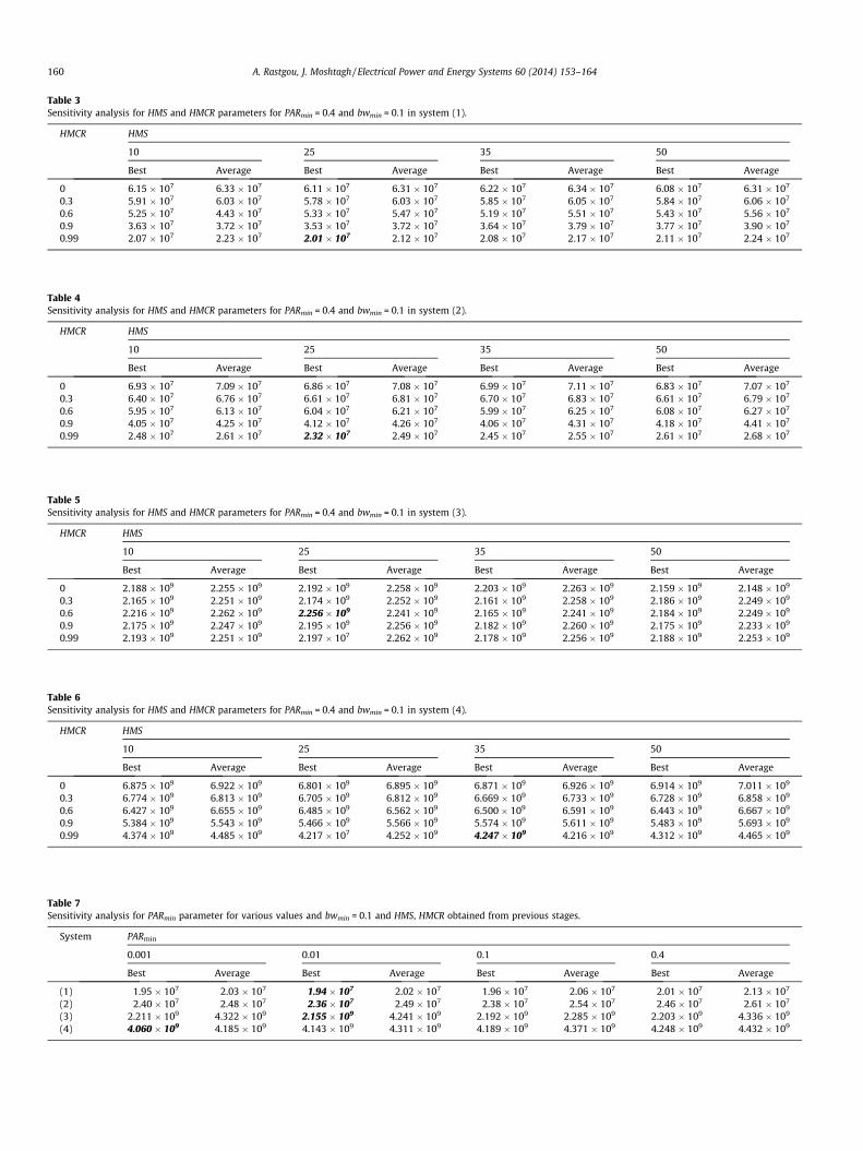
in finding the optimum solution of the problem, HMCR, HMS,PARmin and bwmin are varied within their permissible range bykeeping the rest parameters constant to the aforementioned val-ues. For implementation of improved Harmony search algorithm,first sensitivity analysis on the four efficacy parameters HMS,HMCR, PARmin and bwmin were done. Other parameters of the algo-

rithm like bwmax and PARmax are the constant values 0.9 and 0.99,have been considered respectively. The number of iterations forsimulation is considered 10,000. To obtain optimal values for eachparameter, the algorithm has been implemented 25 times and thebest values of the objective function with its mean in the presentedtables. In this analysis, the IEEE 24-bus test system without

Table 3Sensitivity analysis for HMS and HMCR parameters for PARmin = 0.4 and bwmin = 0.1 in system (1).

HMCR HMS

10 25 35 50

Best Average Best Average Best Average Best Average

0 6.15 � 107 6.33 � 107 6.11 � 107 6.31 � 107 6.22 � 107 6.34 � 107 6.08 � 107 6.31 � 107

0.3 5.91 � 107 6.03 � 107 5.78 � 107 6.03 � 107 5.85 � 107 6.05 � 107 5.84 � 107 6.06 � 107

0.6 5.25 � 107 4.43 � 107 5.33 � 107 5.47 � 107 5.19 � 107 5.51 � 107 5.43 � 107 5.56 � 107

0.9 3.63 � 107 3.72 � 107 3.53 � 107 3.72 � 107 3.64 � 107 3.79 � 107 3.77 � 107 3.90 � 107

0.99 2.07 � 107 2.23 � 107 2.01 � 107 2.12 � 107 2.08 � 107 2.17 � 107 2.11 � 107 2.24 � 107

Table 4Sensitivity analysis for HMS and HMCR parameters for PARmin = 0.4 and bwmin = 0.1 in system (2).

HMCR HMS

10 25 35 50

Best Average Best Average Best Average Best Average

0 6.93 � 107 7.09 � 107 6.86 � 107 7.08 � 107 6.99 � 107 7.11 � 107 6.83 � 107 7.07 � 107

0.3 6.40 � 107 6.76 � 107 6.61 � 107 6.81 � 107 6.70 � 107 6.83 � 107 6.61 � 107 6.79 � 107

0.6 5.95 � 107 6.13 � 107 6.04 � 107 6.21 � 107 5.99 � 107 6.25 � 107 6.08 � 107 6.27 � 107

0.9 4.05 � 107 4.25 � 107 4.12 � 107 4.26 � 107 4.06 � 107 4.31 � 107 4.18 � 107 4.41 � 107

0.99 2.48 � 107 2.61 � 107 2.32 � 107 2.49 � 107 2.45 � 107 2.55 � 107 2.61 � 107 2.68 � 107

Table 5Sensitivity analysis for HMS and HMCR parameters for PARmin = 0.4 and bwmin = 0.1 in system (3).

HMCR HMS

10 25 35 50

Best Average Best Average Best Average Best Average

0 2.188 � 109 2.255 � 109 2.192 � 109 2.258 � 109 2.203 � 109 2.263 � 109 2.159 � 109 2.148 � 109

0.3 2.165 � 109 2.251 � 109 2.174 � 109 2.252 � 109 2.161 � 109 2.258 � 109 2.186 � 109 2.249 � 109

0.6 2.216 � 109 2.262 � 109 2.256 � 109 2.241 � 109 2.165 � 109 2.241 � 109 2.184 � 109 2.249 � 109

0.9 2.175 � 109 2.247 � 109 2.195 � 109 2.256 � 109 2.182 � 109 2.260 � 109 2.175 � 109 2.233 � 109

0.99 2.193 � 109 2.251 � 109 2.197 � 107 2.262 � 109 2.178 � 109 2.256 � 109 2.188 � 109 2.253 � 109

Table 6Sensitivity analysis for HMS and HMCR parameters for PARmin = 0.4 and bwmin = 0.1 in system (4).

HMCR HMS

10 25 35 50

Best Average Best Average Best Average Best Average

0 6.875 � 109 6.922 � 109 6.801 � 109 6.895 � 109 6.871 � 109 6.926 � 109 6.914 � 109 7.011 � 109

0.3 6.774 � 109 6.813 � 109 6.705 � 109 6.812 � 109 6.669 � 109 6.733 � 109 6.728 � 109 6.858 � 109

0.6 6.427 � 109 6.655 � 109 6.485 � 109 6.562 � 109 6.500 � 109 6.591 � 109 6.443 � 109 6.667 � 109

0.9 5.384 � 109 5.543 � 109 5.466 � 109 5.566 � 109 5.574 � 109 5.611 � 109 5.483 � 109 5.693 � 109

0.99 4.374 � 109 4.485 � 109 4.217 � 107 4.252 � 109 4.247 � 109 4.216 � 109 4.312 � 109 4.465 � 109

Table 7Sensitivity analysis for PARmin parameter for various values and bwmin = 0.1 and HMS, HMCR obtained from previous stages.

System PARmin

0.001 0.01 0.1 0.4

Best Average Best Average Best Average Best Average

(1) 1.95 � 107 2.03 � 107 1.94 � 107 2.02 � 107 1.96 � 107 2.06 � 107 2.01 � 107 2.13 � 107

(2) 2.40 � 107 2.48 � 107 2.36 � 107 2.49 � 107 2.38 � 107 2.54 � 107 2.46 � 107 2.61 � 107

(3) 2.211 � 109 4.322 � 109 2.155 � 109 4.241 � 109 2.192 � 109 2.285 � 109 2.203 � 109 4.336 � 109

(4) 4.060 � 109 4.185 � 109 4.143 � 109 4.311 � 109 4.189 � 109 4.371 � 109 4.248 � 109 4.432 � 109

160 A. Rastgou, J. Moshtagh / Electrical Power and Energy Systems 60 (2014) 153–164

Table 8Sensitivity analysis for bwmin parameters for various values HMS, HMCR and PARmin obtained from previous stages.

System bwmin

0.0001 0.01 0.1 0.4

Best Average Best Average Best Average Best Average

(1) 7.95 � 106 8.79 � 106 7.93 � 106 8.55 � 106 1.96 � 107 2.04 � 107 3.30 � 107 3.46 � 107

(2) 1.09 � 107 1.21 � 107 1.16 � 107 1.27 � 107 2.31 � 107 2.49 � 107 3.64 � 107 3.85 � 107

(3) 2.083 � 109 2.158 � 109 2.137 � 109 2.208 � 109 2.192 � 109 2.215 � 109 2.158 � 109 2.248 � 109

(4) 2.809 � 109 3.001 � 109 2.874 � 109 2.934 � 109 2.874 � 109 4.301 � 109 5.061 � 109 5.174 � 109

1t =

2t =

2

1 2−

L

...0 03 2 0

1 3− 1 5− 14 23− 16 23− 19 23−

1 1 2 000 ...

Fig. 5. Codification of solutions.

Table 9Comparison of computational time between HSA and GA for the two systemsconsidered.

System Time (min)

HSA GA

(1) 3.42 5.03(2) 6.11 10.06(3) 20.23 30.40(4) 38.01 50.47

Table 11TEP results for the IEEE 118-bus system.

Year Corridors to build

HSA GA

Adequacy Security Adequacy Security

1 3–5 3–52 55–56 55–563 8–9 8–945 83–85 55–566 77–78 77–78 30–17, 26–307 8–5, 38–65 38–6589 55–56 77–78, 55–5610 55–56 110–112 38–65, 110–112, 55–56Total Cost (M$) 2083 2809 2333 3542

A. Rastgou, J. Moshtagh / Electrical Power and Energy Systems 60 (2014) 153–164 161

security, IEEE 24-bus test system with security, IEEE 118-bus testsystem without security and IEEE 118-bus test system withsecurity are shown by number of (1)–(4) respectively. From Tables3–6, for systems (1)–(4) it can be seen that large values of theparameter HMCR make convergence algorithm faster. The best val-ues for HMS and HMCR for systems (1) and (2), are 25 and 0.99, forsystem (3) is 35 and 0.3 and for system (4) is 35 and 0.99. In Table 7sensitivity analysis has been done on parameter PARmin with HMCRand HMS that obtained from the previous stage, for systems (1), (2)and (3) this parameter equal to 0.01 and 0.001 for system (4). InTable 8 sensitivity analysis has been done on bwmin parameter

Table 10TEP results for the IEEE 24-bus system.

Year Corridors to build

HSA

Adequacy Security

12 16–19 6–8, 15–163 12–23 14–234 4–9 1–8, 2–85 6–7, 6–10, 1–2 1–8, 6–8, 16–19, 7–2,6 12–23, 1–2,4–97 10–11*, 17–22, 3–9 6–7, 9–11*, 9–12*, 108 4–9, 6–10 6–8, 17–189 10–11* 17–1810 20–23, 16–17 9–11*, 9–12*, 2–6, 6–Total cost (M$) 7.93 10.9

* Is meant to increase the transformer capacity.

for HMCR, HMS and PARmin that obtained from Tables 3–7. Accord-ing to these tables the best mode for bwmin parameter is 0.0001 forsystems (2), (3) and (4), and 0.01 for system (1). This problem wasimplemented using genetic algorithm. Fig. 5 shows the codificationof solutions has been used in this study [39,34]. Every numeric va-lue of each gene in a chromosome corresponds to the number ofnew added lines. The number of the right-of-ways gives the lengthof the chromosomes. In this codification, each solution is repre-sented by a t � l matrix corresponding to t planning stages and lright-of-ways (existing and new right-of-ways). The matrix valuesshow the number of new lines added to the corresponding right-of-way. For example, Fig. 5 shows that two new circuits are addedin right-of-way 1–2 in stage one, and one circuit is also added tothis right-of-way in stage two. Objective function is consideredas the fitness function. Since each chromosome represents a net-work expansion plan, a higher fitness is equal to better design. Inthis paper the crossover operator is performed in such way thateach child (child 1 and child 2) produced from parents as in (16):

GA

Adequacy Security

19–23 1–5, 2–419–20 8–92–8 9–12*

9–11* 17–18, 10–11*

19–23 6–8, 10–12*, 17–22 9–12, 11–14, 7–2, 20–231–2, 1–3, 1–5 9–12*, 10–12*

–11* 9–11*, 9–12* 3–9, 3–24, 11–1316–23 8–10, 17–22, 21–226–10, 12–14 17–22, 16–19, 10–11*

10 10–12* 11–13, 9–12*, 6–88.03 12.4

0 1000 2000 3000 4000 5000 6000 7000 8000 9000 10000

2

4

6

8

10x 106

Iteration

Cos

t ($/

year

)

(a)

0 1000 2000 3000 4000 5000 6000 7000 8000 9000 100000

2

4

6

8

10x 106

Cos

t ($/

year

)

Iteration(b)

Fig. 6. Optimization procedure by (a) HSA, (b) GA, for system (1).

0 1000 2000 3000 4000 5000 6000 7000 8000 9000 100002

2.2

2.4

2.6

2.8

3

x 109

Iteration

Cos

t ($/

year

)

(a)

0 1000 2000 3000 4000 5000 6000 7000 8000 9000 10000

2.4

2.6

2.8

3

3.2

3.4

x 109

Iteration

Cos

t ($/

year

)

(b)

Fig. 7. Optimization procedure by (a) HSA, (b) GA, for system (3).

1 2 3 4 5 6 7 8 9 100

5

10

15

20

25

30

Unit

LMP

($/M

wh)

GAHSA

Fig. 8. The comparison of LMPs between HAS and GA for system (1).

0 10 20 30 40 50 6044

45

46

47

48

49

Unit

LMP

($/M

wh)

HSAGA

Fig. 9. The comparison of LMPs between HAS and GA for system (3).

0 10 20 30 40 50 6042

44

46

48

50

52

54

56

Unit

LMP

($/M

wh)

not plannedplanned

Fig. 10. Comparison of the LMPs at each unit for system (4).

162 A. Rastgou, J. Moshtagh / Electrical Power and Energy Systems 60 (2014) 153–164

child 1 ¼ j½C � parent1þ ð1� CÞ � parent 2�jchild 2 ¼ j½C � parent 2þ ð1� CÞ � parent 1�j

ð16Þ

where C is a random number in the range between zero and one.|[.]| Operator is bracket function. Mutation operator is to be per-formed that if the corresponding scheme of a chromosome is over-load, a mutation gene whose value is less than its maximum israndomly chosen and its gene value is increased, i.e., adding lines.Otherwise, a mutation gene whose value is more than zero is se-lected and its gene value is decreased, i.e., reducing lines. Table 9shows the comparison of computational time between HSA andGA for the two systems considered. The best results of the HSAand GA have been presented in Tables 10 and 11. In Figs. 6 and 7for systems (1), (3) the rate of change objective function versusnumber of iterations for both algorithms are illustrated. In Figs. 8and 9 comparison of LMPs between HSA and GA for the two systems(1), (3) has been considered. However, notice that the objective ofpower system planning is to maximize the social welfare, not tominimize the LMPs. Therefore the planned system does not

A. Rastgou, J. Moshtagh / Electrical Power and Energy Systems 60 (2014) 153–164 163

necessarily have lower LMPs at every unit. The DC model based LMPprofile of the initial network with and without additional lines atthe end of the horizon is compared in Fig. 10. One can observe thatthe LMPs for the planned system at the end of the horizon are muchflatter than not planned for system (4). This is because more con-gestion in system exists initially.

5. Conclusion

In this paper, by expanding harmony search method, as one ofthe latest evolutionary algorithms, a new methodology is pre-sented for solving transmission expansion planning problem. Inthe proposed model in addition to construction’s costs, which isa fundamental part of TEP, congestion cost and security cost arealso considered. The proposed methodology and genetic algorithmare applied on the IEEE 24-bus and IEEE 118-bus test systems. Thetransmission expansion plans resulted from each algorithm arealso presented and compared. According to obtained results theproposed algorithm has a less investment cost rather than the ge-netic algorithm. It is worth mentioning that the proposed methodis a better algorithm regarding its convergence rate. Simulation re-sults show that the proposed approach is accurate and efficient,and has the potential to be applied to large scale power systemplanning problems.

References

[1] Zhang H, Vittal V, Heydt GT, Quintero J. A mixed-integer linear programmingapproach for multi-stage security-constrained transmission expansionplanning. Power Syst, IEEE Trans 2012;27:1125–33.

[2] Latorre G, Cruz RD, Areiza JM, Villegas A. Classification of publications andmodels on transmission expansion planning. Power Syst, IEEE Trans2003;18:938–46.

[3] Hashimoto S, Romero R, Mantovani J. Efficient linear programming algorithmfor the transmission network expansion planning problem. Generation,transmission and distribution, IEE proceedings: IET; 2003. p. 536–42.

[4] Shayeghi H, Bagheri A. Dynamic sub-transmission system expansion planningincorporating distributed generation using hybrid DCGA and LP technique. Int JElectr Power Energy Syst 2013;48:111–22.

[5] Dusonchet Y, El-Abiad A. Transmission planning using discrete dynamicoptimizing. Power Apparatus Syst, IEEE Trans 1973:1358–71.

[6] Youssef H, Hackam R. New transmission planning model. Power Syst, IEEETrans 1989;4:9–18.

[7] Asadamongkol S, Eua-arporn B. Transmission expansion planning with ACmodel based on generalized benders decomposition. Int J Electr Power EnergySyst 2013;47:402–7.

[8] Bahiense L, Oliveira GC, Pereira M, Granville S. A mixed integer disjunctivemodel for transmission network expansion. Power Syst, IEEE Trans2001;16:560–5.

[9] Dewani B, Daigavane M, Zadgaonkar A. A review of various computationalintelligence techniques for transmission network expansion planning. Powerelectronics, drives and energy Systems (PEDES), 2012 IEEE InternationalConference: IEEE; 2012. p. 1–5.

[10] Hemmati R, Hooshmand R-A, Khodabakhshian A. State-of-the-art oftransmission expansion planning: comprehensive review. Renew SustainEnergy Rev 2013;23:312–9.

[11] Handschin E, Heine M, Konig D, Nikodem T, Seibt T, Palma R. Object-orientedsoftware engineering for transmission planning in open access schemes.Power Syst, IEEE Trans 1998;13:94–100.

[12] Gallego R, Alves A, Monticelli A, Romero R. Parallel simulated annealingapplied to long term transmission network expansion planning. Power Syst,IEEE Trans 1997;12:181–8.

[13] Da Silva EL, Ortiz JA, De Oliveira GC, Binato S. Transmission network expansionplanning under a tabu search approach. Power Syst, IEEE Trans 2001;16:62–8.

[14] Gallego RA, Romero R, Monticelli AJ. Tabu search algorithm for networksynthesis. Power Syst, IEEE Trans 2000;15:490–5.

[15] Wen F, Chang C. Transmission network optimal planning using the tabu searchmethod. Electric Power Syst Res 1997;42:153–63.

[16] Babic AB, Saric AT, Rankovic A. Transmission expansion planning based onlocational marginal prices and ellipsoidal approximation of uncertainties. Int JElectr Power Energy Syst 2013;53:175–83.

[17] Miranda V, Proença LM. Probabilistic choice vs. risk analysis-conflicts andsynthesis in power system planning. Power industry computer applications,1997 20th international conference: IEEE; 1997. p. 16–21.

[18] Mahdavi M, Shayeghi H, Kazemi A. DCGA based evaluating role of bundle linesin TNEP considering expansion of substations from voltage level point of view.Energy Convers Manage 2009;50:2067–73.

[19] Foroud AA, Abdoos AA, Keypour R, Amirahmadi M. A multi-objectiveframework for dynamic transmission expansion planning in competitiveelectricity market. Int J Electr Power Energy Syst 2010;32:861–72.

[20] Mahmoudabadi A, Rashidinejad M. An application of hybrid heuristic methodto solve concurrent transmission network expansion and reactive powerplanning. Int J Electr Power Energy Syst 2013;45:71–7.

[21] Teive R, Silva E, Fonseca L. A cooperative expert system for transmissionexpansion planning of electrical power systems. Power Syst, IEEE Trans1998;13:636–42.

[22] Sun H, Yu D. A multiple-objective optimization model of transmissionenhancement planning for independent transmission company (ITC). Powerengineering society summer meeting, 2000 IEEE: IEEE; 2000. p. 2033–8.

[23] Silva Sousa A, Asada EN. Combined heuristic with fuzzy system totransmission system expansion planning. Electric Power Syst Res2011;81:123–8.

[24] Kamyab G-R, Fotuhi-Firuzabad M, Rashidinejad M. A PSO based approach formulti-stage transmission expansion planning in electricity markets. Int J ElectrPower Energy Syst 2014;54:91–100.

[25] Shayeghi H, Mahdavi M, Bagheri A. An improved DPSO with mutation based onsimilarity algorithm for optimization of transmission lines loading. EnergyConvers Manage 2010;51:2715–23.

[26] Shayeghi H, Mahdavi M, Bagheri A. Discrete PSO algorithm based optimizationof transmission lines loading in TNEP problem. Energy Convers Manage2010;51:112–21.

[27] Leite da Silva AM, Rezende LS, da Fonseca Manso LA, de Resende LC. Reliabilityworth applied to transmission expansion planning based on ant colonysystem. Int J Electr Power Energy Syst 2010;32:1077–84.

[28] Escobar AH, Gallego RA, Romero R. Multistage and coordinated planning of theexpansion of transmission systems. Power Syst, IEEE Trans 2004;19:735–44.

[29] Romero R, Rocha C, Mantovani J, Sánchez I. Constructive heuristic algorithmfor the DC model in network transmission expansion planning. Generation,transmission and distribution, IEE proceedings: IET; 2005. p. 277–82.

[30] Romero R, Monticelli A, Garcia A, Haffner S. Test systems and mathematicalmodels for transmission network expansion planning. IEE Proc-Generation,Transm Distribution 2002;149:27–36.

[31] Ekwue A, Cory B. Transmission system expansion planning by interactivemethods. Power Apparatus Syst, IEEE Trans 1984:1583–91.

[32] Haffner S, Monticelli A, Garcia A, Mantovani J, Romero R. Branch and boundalgorithm for transmission system expansion planning using a transportationmodel. IEE Proc-Generation, Transm Distribution 2000;147:149–56.

[33] Haffner S, Monticelli A, Garcia A, Romero R. Specialised branch-and-boundalgorithm for transmission network expansion planning. Generation,transmission and distribution, IEE Proceedings: IET; 2001. p. 482–8.

[34] Romero R, Rocha C, Mantovani M, Mantovani J. Analysis of heuristic algorithmsfor the transportation model in static and multistage planning in networkexpansion systems. Generation, transmission and distribution, IEEProceedings: IET; 2003. p. 521–6.

[35] Romero R, Gallego R, Monticelli A. Transmission system expansion planning bysimulated annealing. Power Syst, IEEE Trans 1996;11:364–9.

[36] Gallego R, Monticelli A, Romero R. Transmission system expansion planning byan extended genetic algorithm. Generation, transmission and distribution, IEEProceedings: IET; 1998. p. 329–35.

[37] Al-Saba T, El-Amin I. The application of artificial intelligent tools to thetransmission expansion problem. Electric Power Syst Res 2002;62:117–26.

[38] Rider M, Garcia A, Romero R. Transmission system expansion planning by abranch-and-bound algorithm. Generation, Transm Distribution, IET2008;2:90–9.

[39] Silva IdJ, Rider MJ, Romero R, Murari CA. Genetic algorithm of Chu and Beasleyfor static and multistage transmission expansion planning. Power EngineeringSociety General Meeting, 2006 IEEE: IEEE; 2006. p. 7.

[40] Asada EN, Carreno E, Romero R, Garcia AV. A branch-and-bound algorithm forthe multi-stage transmission expansion planning. Power Engineering SocietyGeneral Meeting, 2005 IEEE: IEEE; 2005. p. 171–6.

[41] Leou R-C. A multi-year transmission planning under a deregulated market. IntJ Electr Power Energy Syst 2011;33:708–14.

[42] Geem ZW, Kim JH, Loganathan G. A new heuristic optimization algorithm:harmony search. Simulation 2001;76:60–8.

[43] Lee KS, Geem ZW. A new structural optimization method based on theharmony search algorithm. Comput Struct 2004;82:781–98.

[44] Afkousi-Paqaleh M, Rashidinejad M, Pourakbari-Kasmaei M. Animplementation of harmony search algorithm to unit commitment problem.Electr Eng 2010;92:215–25.

[45] Vasebi A, Fesanghary M, Bathaee S. Combined heat and power economicdispatch by harmony search algorithm. Int J Electr Power Energy Syst2007;29:713–9.

[46] Parizad A, Baghaee H, Dehghan S, Kiyani B. Application of harmony search fortransmission expansion planning considering security index and uncertainty.Electric Power and Energy Conversion Systems, 2009 EPECS’09 InternationalConference: IEEE; 2009. p. 1–8.

[47] Verma A, Panigrahi B, Bijwe P. Harmony search algorithm for transmissionnetwork expansion planning. Generation, Trans Distribution, IET2010;4:663–73.

[48] Shrestha G, Fonseka P. Congestion-driven transmission expansion incompetitive power markets. Power Syst, IEEE Trans 2004;19:1658–65.

[49] Christie RD, Wollenberg BF, Wangensteen I. Transmission management in thederegulated environment. Proc IEEE 2000;88:170–95.

164 A. Rastgou, J. Moshtagh / Electrical Power and Energy Systems 60 (2014) 153–164

[50] Buygi MO, Balzer G, Shanechi HM, Shahidehpour M. Market-basedtransmission expansion planning. Power Syst, IEEE Trans 2004;19:2060–7.

[51] Bazaraa MS, Jarvis JJ, Sherali HD. Linear programming and networkflows. Wiley-Interscience; 2011.

[52] Luenberger DG. Introduction to linear and nonlinear programming; 1973.[53] Boyd SP, Vandenberghe L. Convex optimization. Cambridge university press;

2004.[54] North American Electric Reliability Council (NERC). (1997, Nov.) GAPP

experiment, six month report. <http://www.nerc.com>.[55] Lee KS, Geem ZW. A new meta-heuristic algorithm for continuous engineering

optimization: harmony search theory and practice. Comput Methods ApplMech Eng 2005;194:3902–33.

[56] Mahdavi M, Fesanghary M, Damangir E. An improved harmony searchalgorithm for solving optimization problems. Appl Math Comput2007;188:1567–79.

[57] Maghouli P, Hosseini SH, Buygi MO, Shahidehpour M. A multi-objectiveframework for transmission expansion planning in deregulated environments.Power Syst, IEEE Trans 2009;24:1051–61.

[58] Grigg C, Wong P, Albrecht P, Allan R, Bhavaraju M, Billinton R, et al. The IEEEreliability test system-1996. A report prepared by the reliability test systemtask force of the application of probability methods subcommittee. Power Syst,IEEE Trans 1999;14:1010–20.

[59] Fang R, Hill DJ. A new strategy for transmission expansion in competitiveelectricity markets. Power Syst, IEEE Trans 2003;18:374–80.

[60] Electrical and Computer Engineering Department, Illinois Institute ofTechnology (IIT), IEEE 118-Bus System Data. <http://motor.ece.iit.edu/Data/JEAS_IEEE118.doc>.