July 2006 CEA - Bruyères-le-Châtel Improved predictive sampling using quasi-Monte Carlo with application to neutron-cross-section evaluation Ken Hanson T-16, Nuclear Physics; Theoretical Division Los Alamos National Laboratory This presentation available at http://kmh-lanl.hansonhub.com LA-UR-05-3096
Transcript
July 2006 CEA - Bruyères-le-Châtel 1
Improved predictive sampling using quasi-Monte Carlo with application to
neutron-cross-section evaluation
Ken HansonT-16, Nuclear Physics; Theoretical Division
Los Alamos National Laboratory
This presentation available at http://kmh-lanl.hansonhub.com
LA-UR-05-3096
July 2006 CEA - Bruyères-le-Châtel 2
Collaborators and counselors Toshihiko Kawano, Patrick Talou, Mark Chadwick
Stephanie Frankle, Bob Little
Mike Fitzpatrick, David Haynor, Dave Brown, Brandon Gallas
Chris Orum, Bill Press
Dave Higdon, Brian Williams, Rick Picard, David Mease, Mike McKay
Max Gunzburger, Vicente Romero, Steve Wojtkiewicz
Tony Warnock, Paul Pederson
July 2006 CEA - Bruyères-le-Châtel 3
Overview• Quasi-Monte Carlo (QMC) – purpose • Digital halftoning – purpose and constraints• New approaches to generating sample sets with uniform spacing
► halftoning algorithm provides good point sets for QMC► leads to Repulsive Particle Model (RPM) and Centroidal Voronoi
Tessellation (CVT)
• Point sets for sampling distributions in high dimensions► predictive sampling – estimate prediction mean and uncertainty
• Neutron cross-section evaluation► combine directly measured neutron cross sections for fission of 239Pu
with a high-accuracy criticality measurement► Bayesian update► objective – to characterize prediction uncertainty using 30 samples for 30
input parameters
July 2006 CEA - Bruyères-le-Châtel 4
Context – big physics simulation codes• Computer simulation codes
► many input parameters, many output variables► very expensive to run; days to weeks on super computers
• Important to assess uncertainties in predictions -thus need to ► compare codes to experimental data; make inferences► use advanced methods to estimate sensitivity of simulation outputs to inputs
• Latin square (hypercube), stratified sampling, quasi-Monte Carlo, CVT
• Examples of complex simulations► nuclear-reactor design ► ocean and atmosphere modeling► aircraft design; space shuttle design► casting of metals
calculations can take 3 months!
July 2006 CEA - Bruyères-le-Châtel 5
Our application• Focus on neutron cross sections• Aim to improve our knowledge of
the cross sections by incorporating a high-precision criticality measurement; integral constraint
• Criticality experiment simulated with a discrete-ordinate code, based on 30 energy bins
• Ultimate goal is to use the improved cross sections to predict other similar physical situations
• Need to characterize prediction uncertainties; 30-D parameter space
Criticality experiment
Neutron fission cross section
July 2006 CEA - Bruyères-le-Châtel 6
Monte Carlo integration techniques• Generic purpose of Monte Carlo
► estimate integral of a function over a specified region R in m dimensions, based on evaluations at n sample points
• Constraints► integrand not available in analytic form, but calculable► function evaluations may be expensive, so minimize number
• Algorithmic approaches – want best accuracy with fixed number of function evaluations n► simple quadrature (Riemann sum) – good for few dimensions; rms err ~ n-1
► Monte Carlo – useful for many dimensions; rms err ~ n-1/2
► quasi-Monte Carlo – reduce number of evaluations; rms err ~ n-1
1
( ) ( )n
ii
x x x=
= ∑∫ R
R
Vf d fn
July 2006 CEA - Bruyères-le-Châtel 7
Quasi-Monte Carlo• Purpose
► estimate integral of a function over a specified domainin d dimensions
► obtain better rate of convergence of integral estimation than occurs in classic Monte Carlo
• Constraints► integrand function not available analytically, but calculable► function known (or assumed) to be reasonably well behaved, e.g. smooth
• Standard QMC approaches use low-discrepancy sequences; product space (Halton, Sobel, Faure, Hammersley, …)► most studies usually involve many samples in a few dimensions
• Propose here new ways of generating sample point sets► our focus is on a few samples in high dimensions
July 2006 CEA - Bruyères-le-Châtel 8
Point set examples (2-D)• Scatter plots of different kinds of point sets (400 points)• Halton sequence reduces clustering that occurs in random seqs.• If quasi-MC sequences have better integration properties than
random, . . . is halftone pattern even better?
Random(independent)
Quasi-Random (Halton sequence)
Halftone(DBS sky)
July 2006 CEA - Bruyères-le-Châtel 9
Digital halftoning techniques• Purpose
► render a gray-scale image by placing black dots on white background► make halftone rendering look like original gray-scale image► related to characteristics of human observer► important for laser printers
• Constraints► resolution – size and closeness of dots, number of dots► speed of rendering
• Various algorithmic approaches► error diffusion, look-up tables, blue-noise, …► concentrate here on Direct Binary Search (Allebach et al.)
July 2006 CEA - Bruyères-le-Châtel 10
Direct Binary Search example• DBS produces halftone images
with excellent visual quality• Sky region has uniform density;
quasi-random pattern • Computationally intensive
Li and Allebach, IEEE Trans. Image Proc. 9, 1593-1603 (2000)
July 2006 CEA - Bruyères-le-Châtel 11
Direct Binary Search (DBS) algorithm• Consider digital halftone image to be composed of black or
white pixels• Cost function is based on perception of two images
► where d is the dot image, g is the gray-scale image to be rendered, * represents convolution, and h is the image of the blur function of the human eye, for example,
• To minimize φ► start with a collection of dots with average local density ~ g► iterate sequentially through all image pixels;► for each pixel, swap value with neighborhood pixels, or toggle its value to
reduce φ
• Edge effects must be dealt with► in above, dot image surrounded by field of uniform density
2( )ϕ = ∗ −h d g
3/ 2( )−2 2w + r
July 2006 CEA - Bruyères-le-Châtel 12
Minimum Visual Discrepancy (MVD) algorithmInspired by Direct Binary Search halftoning algorithm:
• Start with an initial set of points• Goal is to create uniformly distributed set of points• Cost function is variance in blurred point image
► where d is the point (dot) image, h is the blur function of the human eye, and * represents convolution
• Minimize ψ by► starting with some point set (random, stratified, Halton,…)► visiting each point in random order;► moving each point in 8 directions, and accept move that lowers ψ the
most
var( )ψ = ∗h d
July 2006 CEA - Bruyères-le-Châtel 13
Minimum Visual Discrepancy (MVD) algorithm• MVD result; start with 95 points from Halton sequence• MVD objective is to minimize variance in blurred image• Effect is to force points to be evenly distributed, or as far apart
from each other as possible• Might expect global minimum is a regular pattern
MVD, 95 Blurred image
July 2006 CEA - Bruyères-le-Châtel 14
MVD results• In each optimization, final pattern depends on initial point set
► algorithm seeks local minimum, not global (as does DBS)
• Patterns somewhat resemble regular hexagonal array► similar to lattice structure in crystals or glass► however, lack long-range (coarse scale) order► best to start with point set with good long-range uniformity
MVD, 1000MVD, 400MVD, 95
July 2006 CEA - Bruyères-le-Châtel 15
Point set examples• Compare various kinds of point sets (400 points)
► varying degrees of randomness and uniformity
• As the points become more uniformly distributed, the more accurate are the values of estimated integrals
• Example:
MVD, 0.14%Halton, 0.5%Random, 2.5% Grid, 0.09%
More Uniform, Higher Accuracy
RMS relative accuracies of integral of ( )0 0func2= exp 2 ; 0 1i i ii
x x x− − < <∏
July 2006 CEA - Bruyères-le-Châtel 16
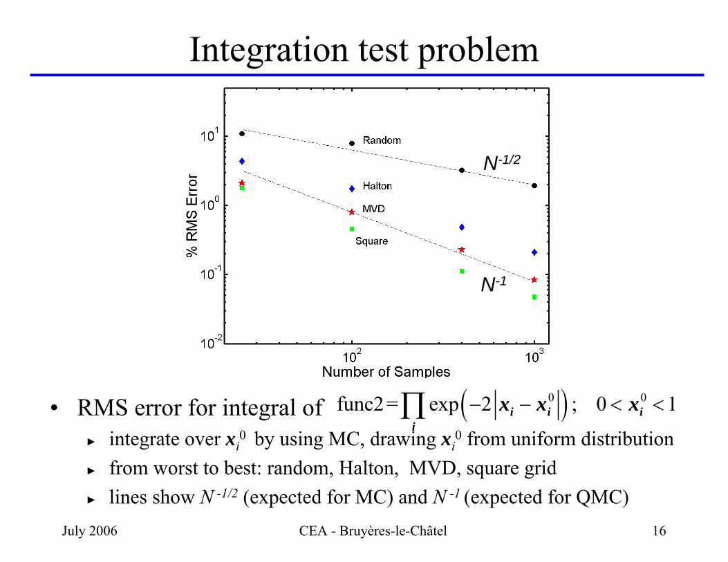
Integration test problem
• RMS error for integral of ► integrate over xi
0 by using MC, drawing xi0 from uniform distribution
► from worst to best: random, Halton, MVD, square grid► lines show N -1/2 (expected for MC) and N -1 (expected for QMC)
( )0 0func2= exp 2 ; 0 1i i ii
x x x− − < <∏
N-1/2
N-1
July 2006 CEA - Bruyères-le-Châtel 17
Marginals for MVD points• Sometimes desirable for
projections of high dimensional point sets to sample each parameter uniformly
• Latin hypercube sampling designed to achieve this property (for specified number of points)
• Plot shows histogram of 95 MVD samples along x-axis, i.e., marginalized over y direction
• MVD points have relatively uniform marginal distributions
MVD, 95 points
marginal
July 2006 CEA - Bruyères-le-Châtel 18
Another use of MVD: visualization of flow field• Fluid flow often visualized as field of vectors• Location of vector bases may be chosen as
► square grid (typical) - regular pattern produces visual artifacts► random points - fewer artifacts, but nonuniform placement► quasi-random - fewest artifacts and uniform placement
Random pointsSquare gridQuasi-random (MVD)
point set
July 2006 CEA - Bruyères-le-Châtel 19
Repulsive particle model• Model points as set of interacting (repulsive) particles• Cost function is the potential
► where V is a particle-particle interaction potential andU is a particle-boundary potential
► particles are repelled by each other and from boundary
• Minimize ψ by moving particles by small steps • This model is analytically equivalent to Minimum Visual
Discrepancy (V and U directly related to blur function h)► related to connection between a field and direct interactions between
particles
• Suitable for generating point sets in high dimensions
, 1
( , ) ( )i j ii j i i
x x xψ≥ +
= +∑ ∑V U
July 2006 CEA - Bruyères-le-Châtel 20
Repulsive particle model• Equivalent to Minimum Visual Discrepancy algorithm• Example of repulsive-particle results
► resulting point pattern is visually indistinguishable from MVD pattern
MVDRepulsive Particle Model
1000 points
July 2006 CEA - Bruyères-le-Châtel 21
Voronoi analysis of point set• Voronoi diagram
► partitions domain into polygons► points in ith polygon are closest
to ith generating point, xi
► boundaries shown are obtained by geometrical construction
• Monte Carlo technique► randomly throw large number of
points zk into region► compute distance of each zk to all
generating points {xi}► zk belongs to Voronoi region of closest xj
► can compute Ai , radial moments, identify neighbors, …
• Readily extensible to high dimensions
Voronoi analysis: 10 random points
Geometric construction
Monte Carlo
July 2006 CEA - Bruyères-le-Châtel 22
Voronoi analysis can improve classic MC• Standard MC formula
• Instead, use weighted average
► where Vi is the volume of Voronoi region for ith point; Riemann integr.
• Accuracy of integral estimate dramatically improved in 2D:► factor of 6.3 for N = 100 (func2)► factor of > 20 for N = 1000 (func2)
• Suitable for adaptive sampling• Less useful in high dimensions (?)
Random, 100
1
( ) ( )x x x=
=∑∫n
i iiR
f d f V
1
( ) ( )x x x=
= ∑∫n
Ri
iR
Vf d fn
July 2006 CEA - Bruyères-le-Châtel 23
Centroidal Voronoi Tessellation• Plot shows 13 random points (·) and the
centroids of their Voronoi regions (×)• A point set is called a Centroidal Voronoi
Tessellation (CVT) when the generating points z j coincide with the centroids their Voronoi regions; a CVT minimizes
• Algorithm (McQueen)► start with arbitrary set of generating points► perform Voronoi analysis using MC algorithm ► move each generating point to its Voronoi centroid► iterate lasts two steps until convergence
• Final CVT points uniformly distributed
Final CVT point set∑ ∫ −
j
j
j
xxz d2
V
Start with random points
July 2006 CEA - Bruyères-le-Châtel 24
Visual comparison of methods• Preceding three algorithms provide uniformly-spaced points,
have essentially equivalent patterns, and are useful for QMC► Minimum Visual Discrepancy (MVD) - halftoning► Repulsive Particle Model (RPM) – physics model► Centroidal Voronoi Tessellation (CVT) - math
• For high dimensions: both CVT and RPM may be useful, RPM likely most efficient
MVD, 95 RPM, 100 CVT, 100
July 2006 CEA - Bruyères-le-Châtel 25
CVT for multi-variate normal distribution• CVT algorithm works for an arbitrary
density function, e.g., a normal distribution
• In above MC algorithm for Voronoi analysis, simply draw random numbers from desired distribution
• Plots show starting random point set and final CVT set
• Radii of points are rescaled to achieve desired average variance along axes
Random, 100
CVT, 100
July 2006 CEA - Bruyères-le-Châtel 26
Recall context• Our interest is in characterizing the uncertainty in a
simulation output, based on uncertainties in the inputs
• But, the high cost of running the simulation limits how many samples can be drawn from a parameter distribution to obtain a predictive distribution
• We are often in a situation where the number of points is comparable to number of parameters (n ≈ d )
• Our goal is to draw a modest number of points from a high-dimensional normal distribution
• Let’s explore some of the characteristics of the problem by starting with the example of 2 sample points in 2D
Simulationx yInputs Outputs
July 2006 CEA - Bruyères-le-Châtel 27
CVT: 2 points in 2 dimensions• Bi-variate normal distribution is
rotationally symmetric• Symmetry of situation means that the
CVT points must be symmetric about origin; at the same radius
• This pattern is unique, up to a random rotation
• Both x1 and x2 values sampled (with near certainty), but there is a subspace, orthogonal to x1-x2 line, whose dependence is not sampled
• Generalizing, the d-D space is under-sampled when n < d + 1
CVT, 2
July 2006 CEA - Bruyères-le-Châtel 28
CVT: 30 points in 30 dimensions• 30 dimensional normal distribution• Projected onto 2D plane, CVT result
doesn’t look much different than random sample set
• However, CVT points are uniformly separated in d-D, while random points are not
CVT, 30Point separation histogram
Random, 30
All points are nearest neighbors!
random
CVT
July 2006 CEA - Bruyères-le-Châtel 29
CVT radial distribution: 30 points in 30D• As with 2 points in 2D, all 30
CVT points in 30D are at the same radius► lie on the surface of a hypersphere
• As seen in last slide, the inter-point distances for CVT are essentially identical► regular point pattern (unique?)
• Rotation is only degree of freedom between different realizations of CVT
• One can generate new CVT patterns by randomly rotating an existing one
n = 30; d = 30
random
CVT
July 2006 CEA - Bruyères-le-Châtel 30
Covariance analysis of point set• Let xj be vector for jth point;
point set is represented by matrix
• Covariance of point set along the axes is XXT
• Eigenanalysis of XXT yields the covariance spectrum► the ith eigenvalue is the variance of the
points projected onto the ith eigenvector
• Conclude that spectrum for CVT point set is much more uniform than for random set, which is quite variable (the Wishart distribution)
• Last eigenvalue is zero; rank = 29
n = 30; d = 301 2 3 n T( ; ; ; )=X x x x x
CVT
random
July 2006 CEA - Bruyères-le-Châtel 31
Linear response model • Assume outputs of a simulation are
linearly related to perturbations in the inputs,where Sy is sensitivity matrix ∂y/∂x
• The covariance in the output y is
► when output y is a scalar, the covariance Cy is a scalar (variance), and Sy is a vector
• If linear model is sufficient and one knows the sensitivity matrix, then predictive distribution is easily characterized
• However, for large simulations, the sensitivity matrix is often unknown
yxyy SCSC T=
Tyδ δ= yS x Simulationx yInputs Outputs
July 2006 CEA - Bruyères-le-Châtel 32
Test single point set using random sensitivities • Assume linear model,
where Sy is sensitivity matrix ∂y/∂x• Test predictive response of a single
sample set for an ensemble of random sensitivity vectors Sy :► Sy= Nd(0,1); mean(Sy) = 0 , var(Sy) = 1► assume input x distribution is
► fissile material 239Pu► measure neutron multiplication as
function of separation of two hemispheres of material
► summarize criticality with neutron multiplication factor, keff = 0.9980 ± 0.0019for a specific geometry
► very accurate measurement
• Our goal – use highly accurate JEZEBEL measurement to improve our knowledge of 239Pu cross sections
JEZEBEL set up
July 2006 CEA - Bruyères-le-Châtel 36
JEZEBEL – sensitivity analysis• PARTISN code relates keff to
neutron cross sections• Sensitivity of keff to cross sections
found by perturbing cross section in each energy bin by 1% and observing increase in keff
• Observe that 1% increase in all cross sections results in 1% increase in keff , as expected
• In real applications, one often does not have this sensitivity vector, so Monte Carlo used to propagate uncertainties
keff sensitivity to cross sections
July 2006 CEA - Bruyères-le-Châtel 37
Bayesian update• For data linearly related to the parameters, the Bayesian
(aka Kalman) update is
► x0 and x1 are parameter vectors before and after update► C0 and C1 are their covariance matrices► y and Cy are the measured data vector and its covariance► y0 is the value of y for x0
► Sy is the matrix of the sensitivity of y to x; ∂y/∂x
• For the JEZEBEL case, y is a scalar (keff), Cy is a scalar (variance), and Sy is a vector
yyy SCSCC 1T10
11
−−− +=
)( 01T
01
011
1 yySCSxCxC yyy −+= −−−
July 2006 CEA - Bruyères-le-Châtel 38
Updated cross sections• Plot shows uncertainties in cross
sections before and after using JEZEBEL measurement
• Modest reduction in uncertainties; follows energy dependence of sensitivity
• Correlation matrix is significantly altered
• Strong negative correlations introduced by integral constraint of matching JEZEBEL’s keff
• Reduced uncertainty may hold only for PARTISN calculations
standard error in cross sections
correlation matrix
July 2006 CEA - Bruyères-le-Châtel 39
Uncertainty in subsequent simulations • Intend to use updated cross sections in new calculations,
with expectation that integral constraint will reduce uncertainties• Use Monte Carlo sampling to estimate the uncertainty in new
predictions; question is “use random MC or qMC?”
• Quasi-MC in form of CVT point sets demonstrated by “predicting”keff measured in JEZEBEL► for this demo, assume linear model with known sensitivity vector► under these assumptions, we can calculate exact answer and compare to MC-
style sampling to obtain predictive distribution• For new physical scenario
► would not have sensitivity vector► full simulation calculation for each MC sample► only a modest number of function evaluations can be done
July 2006 CEA - Bruyères-le-Châtel 40
Rotation matrix in high dimensions• Given unit vectors a and b, want rotation matrix that map a into b• Algorithm (thanks to Mike Fitzpatrick)
► for matrix ► Singular Value Decomposition (SVD) of:
► the bases of the subspace orthogonal to a and b are given by singular vectors in U, except for first two
► then, do SVD on outer product matrix;
► rotation matrix is where D is identity matrix, except
• Random rotations – randomly choose directions of a and b► simple algorithm: randomly draw vector from n-dimensional normal
distribution and normalize it to unit length
T1 VUM Σ=
T1 ) ;( baM =
T2 BAM =
Td43 );; ;( uuuaA = Td43 );; ;( uuubB =
)det(][ T22 VUD =dd
T22 VDUR =
n = 20; d = 6
July 2006 CEA - Bruyères-le-Châtel 41
Examples of rotations in high dimensions• Continuous rotations in various dimensions• Randomly choose directions of rotation• All points have unit radius (on surface of unit hypersphere)
n = 20; d = 4n = 13; d = 3 n = 30; d = 30
July 2006 CEA - Bruyères-le-Châtel 42
Sampling from correlated normal distribution • Want to draw samples from multi-variate normal distribution with
known covariance Cx
• Important to include correlations among uncertainties, i.e., off-diagonal elements
• Algorithm: ► perform eigenanalysis of covariance matrix of d dimensions
where U is orthognal matrix of eigenvectors andΛ is the diagonal matrix of eigenvalues
► draw d samples from unit-variance normal distribution, ξi , to form vector ξ► scale each component of this vector by λi
½
► transform vector into parameter space using the eigenvector matrix► to summarize, correlated parameters are
TUΛUCx =
ξΛUx 1/2=
July 2006 CEA - Bruyères-le-Châtel 43
Accuracy of predicted keff and its uncertainty• Check accuracy of predicted mean and standard deviation based
on 30 samples; CVT vs. random sample sets► exact value from known sensitivity and linear model
• Conclude – CVT is more accurate here than random sampling
Results from 1000 sample sets; ‘rot’ indicates single sample set randomly rotated to achieve each new one
July 2006 CEA - Bruyères-le-Châtel 44
Summary• CVT sampling is useful in predictive sampling for obtaining
higher accuracy for a limited number of simulations
• CVT and repulsive particle model may be used to generate QMC point sets► particularly useful for modest number of points
July 2006 CEA - Bruyères-le-Châtel 45
Future work• Need a way to estimate accuracy of results, a problem common to
all QMC approaches• Important to learn to cope with under-sampling (n < d + 1)
► a parameter subspace dependence is not sampled so some aspects of uncertainty in input parameters may be missed
► satisfactory solution requires careful thought, taking into account what is known about the influence of input parameters on the simulation output
• Sequential generation of point sets► add additional points, keeping previous points fixed
• Adaptive sampling – improve estimate by importance sampling, i.e., increasing density of points in selected regions
• Employ advanced analysis of outputs produced by input samples► weighted Monte Carlo► characterize output response as function of inputs
July 2006 CEA - Bruyères-le-Châtel 46
Covariance analysis of smaller point set• Eigenanalysis of XXT yields the
covariance spectrum► the ith eigenvalue is the variance of the
points projected onto the ith eigenvector
• Conclude that spectrum for CVT point set is much flatter than for random set (Wishart distribution)
• Rank = 9 for both; implies that 21 components of sensitivity vector are not sampled (have zero contribution to result)
n = 10; d = 30
CVT
random
July 2006 CEA - Bruyères-le-Châtel 47
Bibliography ► K. M. Hanson, “Quasi-Monte Carlo: halftoning in high
dimensions?,” Proc. SPIE 5016, pp. 161-172 (2003)► P. Li and J. P. Allebach, “Look-up-table based halftoning
algorithm,” IEEE Trans. Image Proc. 9, pp. 1593-1603 (2000)► H. Niederreiter, Random Number Generation and Quasi-Monte
Carlo Methods (SIAM, 1992)► Q. Du, V. Faber, and M. Gunzburger, “Centroidal Voronoi
tessellations: applications and algorithms,” SIAM Review 41, 637-676 (1999)
► T. Kawano et al., “Combining differential and integral experiments on 239Pu for reducing uncertainties in nuclear data applications,” submitted, 2005
This presentation available at http://kmh-lanl.hansonhub.com