30
Improving Customer Decision in e-Commerce Using Matrix Factorization HENRY OHANGA [CS281-0860/2010]
| Date post: | 14-Aug-2015 |
| Category: |
Software |
| Upload: | henry-ohanga |
| View: | 103 times |
| Download: | 1 times |

Improving Customer Decision in e-Commerce
Using Matrix Factorization
HENRY OHANGA [CS281-0860/2010]

Recap: Online Movie Shop The problem statement:
Too many movies presented to the customer to choose from. Naïve users easily make poor decisions.
Users have divided attention and therefore may not have enough time to make better decisions.
The proposed solution: Provide MORE ACCURATE AND QUALITY MOVIE RECOMMENDATIONS to the
customers.
By inculcating a recommender agent that considers implicit user feedback and temporal effects.
The agent should be able to learn the motivational factors behind customer preferences.

Recap: Online Movie Shop This literature review begs to answer the first four questions asked in the
research proposal document but first builds a general understanding of the recommender systems.
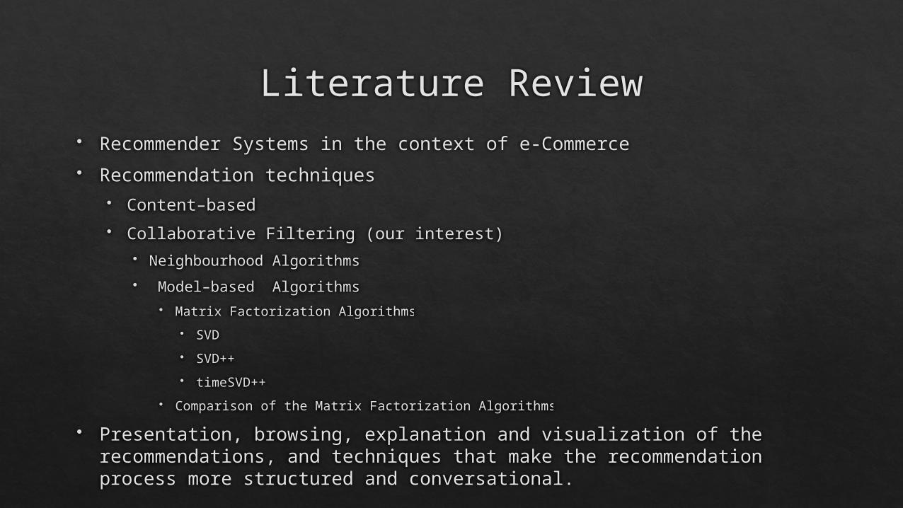
Literature Review Recommender Systems in the context of e-Commerce
Recommendation techniques Content–based
Collaborative Filtering (our interest) Neighbourhood Algorithms
Model–based Algorithms Matrix Factorization Algorithms
SVD
SVD++
timeSVD++
Comparison of the Matrix Factorization Algorithms
Presentation, browsing, explanation and visualization of the recommendations, and techniques that make the recommendation process more structured and conversational.
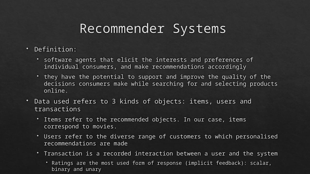
Recommender Systems Definition:
software agents that elicit the interests and preferences of individual consumers, and make recommendations accordingly
they have the potential to support and improve the quality of the decisions consumers make while searching for and selecting products online.
Data used refers to 3 kinds of objects: items, users and transactions Items refer to the recommended objects. In our case, items correspond to movies.
Users refer to the diverse range of customers to which personalised recommendations are made
Transaction is a recorded interaction between a user and the system Ratings are the most used form of response (implicit feedback): scalar, binary and unary
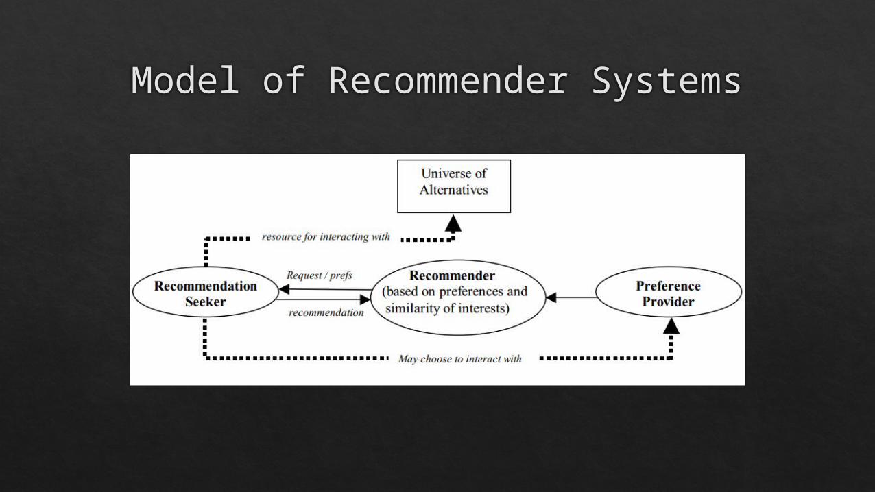
Model of Recommender Systems
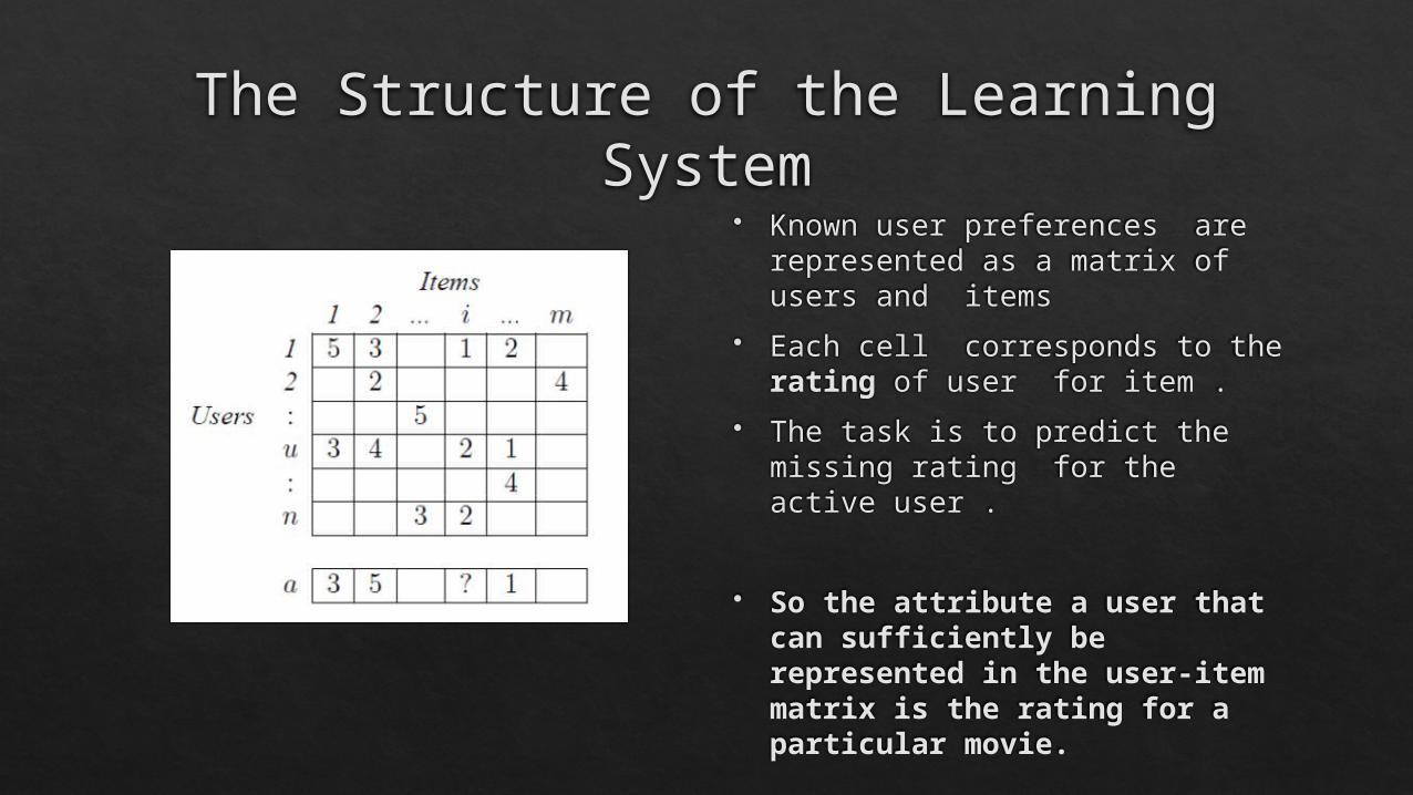
The Structure of the Learning System Known user preferences are
represented as a matrix of users and items
Each cell corresponds to the rating of user for item .
The task is to predict the missing rating for the active user .
So the attribute a user that can sufficiently be represented in the user-item matrix is the rating for a particular movie.

Recommendation Techniques Content-based, Collaborative Filtering, Hybrid Approaches
Content-based Approaches System learns to recommend items that are similar to the ones that the user liked
in the past.
The similarity of items is calculated based on the features associated with the compared items.
For example, if a user has positively rated a movie that belongs to the comedy genre, then the system can learn to recommend other movies from this genre.

Recommendation Techniques Collaborative Filtering Approaches
This approach recommends to the active user the items that other users with similar tastes liked in the past.
The similarity in taste of two users is calculated based on the similarity in the rating history of the users.
The techniques here are broadly categorised into: Neighbourhood Methods (e.g. kNN)
Model-based Methods (e.g. Matrix Factorization)

Neighbourhood Methods Focus on relationships between items or, alternatively, between users
Summary of the Algorithms Assign a weight to all users with respect to similarity with the active user.
Select users that have the highest similarity with the active user – commonly called the neighbourhood.
Compute a prediction from a weighted combination of the selected neighbours’ ratings.

Neighbourhood Methods The similarity metric can be computed using the Pearson correlation
coefficient as
Where is the set of items rated by both users i.e. , is the rating given to item by user , and is the mean rating given by user .
Then, we predict the rating for item by
Where is the prediction for the active user for item , is the similarity between users and , and is the neighbourhood or set of most similar users

Neighbourhood Methods
Limitations Limited coverage
Users can be neighbours only if they have rated common items
But users having rated a few or no common items may still have similar preferences
Also only items rated by neighbours can be recommended
Sensitivity to Sparse data The accuracy of neighbourhood-based recommendation methods suffers from
the lack of available ratings
Users typically rate only a small proportion of the available items
This is aggravated by the fact that users or items newly added to the system may have no ratings at all, a problem known as cold-start.

Improvements to CF Methods Item – based Collaborative Filtering
where is the set of all users who have rated both items and , is the rating of user on item , and is the average rating of the th item across users.
Then, the rating for item for user a can be predicted using a simple weighted average, as in:
where is the neighbourhood set of the items rated by a that are most similar to . For item-based collaborative filtering too, one may use alternative similarity metrics such as adjusted cosine similarity.

Improvements to CF Methods Significance Weighting
Here, we multiply the similarity weight by significance weighting factor, which devalues the correlations based on few co-rated items (Herlocker et al., 1999).
Default Voting Assume a default value for the rating for items that have not been explicitly rated
then compute correlation using the union of items rated by users being matched as opposed to the intersection
Inverse User Frequency Universally liked items or items that have been rated by all users are not as
useful as less common items
It is applied to similarity based CF by multiplying the original rating of item with the factor ; where is the number of users who have rated item out of the total number of users
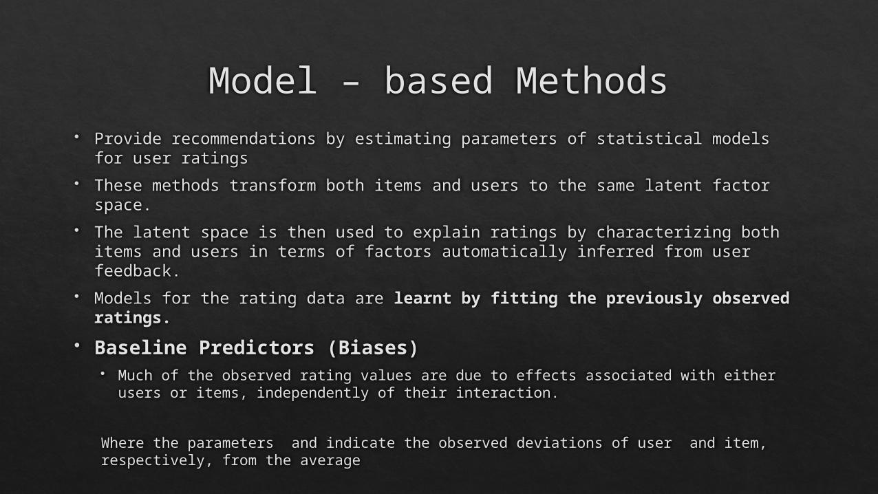
Model – based Methods Provide recommendations by estimating parameters of statistical models for
user ratings
These methods transform both items and users to the same latent factor space.
The latent space is then used to explain ratings by characterizing both items and users in terms of factors automatically inferred from user feedback.
Models for the rating data are learnt by fitting the previously observed ratings.
Baseline Predictors (Biases) Much of the observed rating values are due to effects associated with either users
or items, independently of their interaction.
Where the parameters and indicate the observed deviations of user and item, respectively, from the average
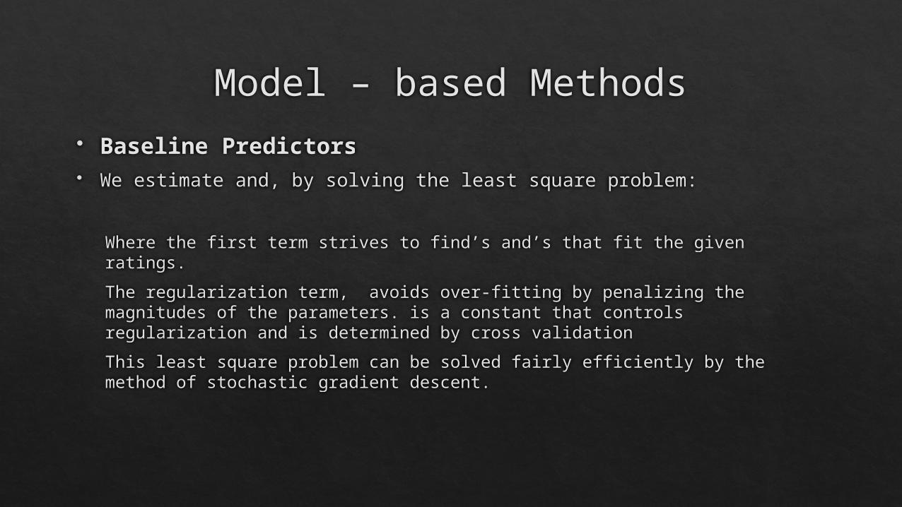
Model – based Methods Baseline Predictors We estimate and, by solving the least square problem:
Where the first term strives to find’s and’s that fit the given ratings.
The regularization term, avoids over-fitting by penalizing the magnitudes of the parameters. is a constant that controls regularization and is determined by cross validation
This least square problem can be solved fairly efficiently by the method of stochastic gradient descent.
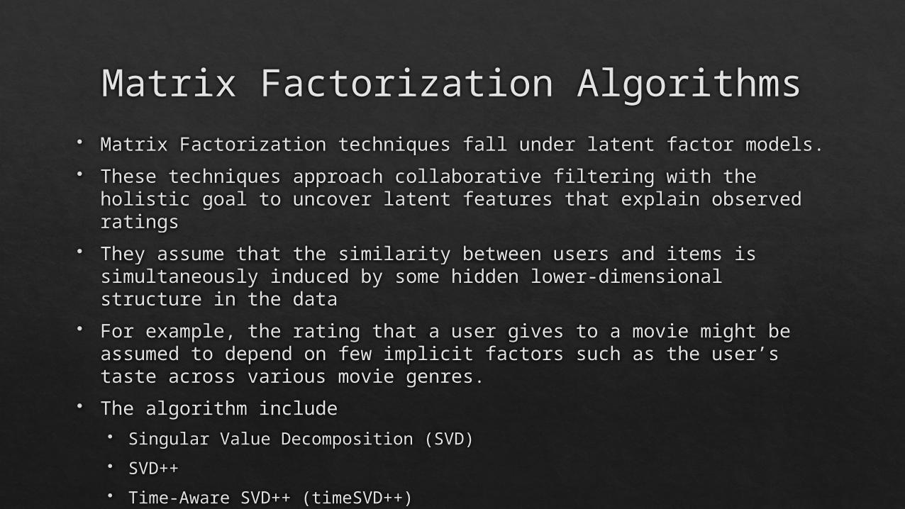
Matrix Factorization Algorithms Matrix Factorization techniques fall under latent factor models.
These techniques approach collaborative filtering with the holistic goal to uncover latent features that explain observed ratings
They assume that the similarity between users and items is simultaneously induced by some hidden lower-dimensional structure in the data
For example, the rating that a user gives to a movie might be assumed to depend on few implicit factors such as the user’s taste across various movie genres.
The algorithm include Singular Value Decomposition (SVD)
SVD++
Time-Aware SVD++ (timeSVD++)

Singular Value Decomposition (SVD) This algorithm is based on a model maps both users and items to a joint latent
factor space of dimensionality, such that user-item interactions are modeled as inner products in that space.
The latent space tries to explain ratings by characterizing both products and users on factors automatically inferred from user feedback
Accordingly, each item is associated with a vector, and each user is associated with a vector.
For a given item, the elements of of measure the extent to which the item possesses those factors, positive or negative.
For a given user, the elements of measure the extent of interest the user has in items that are high on the corresponding factors (again, these may be positive or negative).

Singular Value Decomposition (SVD) The resulting dot product,, captures the interaction between user and item
—i.e., the overall interest of the user in characteristics of the item.
The final rating is created by also adding in the aforementioned baseline predictors that depend only on the user or item.
Thus, a rating is predicted by the rule:
In order to learn the model parameters (,, and ) the algorithm minimizes the regularized squared error:
The constant, which controls the extent of regularization, is usually determined by cross validation. Minimization is typically performed by either stochastic gradient descent or alternating least squares.

Singular Value Decomposition (SVD) The algorithm then loops over all known ratings in, computing:
is a constant representing the learning rate.

SVD++ This algorithm improves on SVD by incorporating implicit user feedback in
learning the user preferences.
It possible to capture a significant signal by accounting for which items the users rate, regardless of their rating value
To this end, a second set of item factors is added, relating each item to a factor vector.
Those new item factors are used to characterize users based on the set of items that they rated. The exact model is represented as:
The set contains the items rated by user.
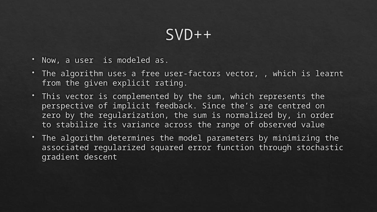
SVD++ Now, a user is modeled as.
The algorithm uses a free user-factors vector, , which is learnt from the given explicit rating.
This vector is complemented by the sum, which represents the perspective of implicit feedback. Since the’s are centred on zero by the regularization, the sum is normalized by, in order to stabilize its variance across the range of observed value
The algorithm determines the model parameters by minimizing the associated regularized squared error function through stochastic gradient descent

SVD++ The algorithm then loops over all known ratings in, computing:

SVD++ Several types of implicit feedback can be simultaneously introduced into the
model by using extra sets of item factors.
For example, if a user has a certain kind of implicit preference to the items in (e.g., she/he bought them), and a different type of implicit feedback to the items in (e.g., she/he browsed them), we could use the model:
The relative importance of each source of implicit feedback will be automatically learned by the algorithm by its setting of the respective values of model parameters.

timeSVD++ This algorithm lends itself well to modeling temporal effects, which
significantly improves prediction accuracy.
It defines a template for a time sensitive baseline predictor for user’s rating of item at day or time:
Here and are real valued functions that change over time, parameterized by temporal effects that either span extended periods of time or more transient effects.
→ split the item biases into time-based bins
→ the linear function to capture a possible gradual drift of user bias
→ smooth functions for modeling the user bias

timeSVD++ Our baseline predictor for modeling the drifting user bias becomes:
To learn the involved parameters, ,, , and, the algorithm solves
Here, the first term strives to construct parameters that fit the given ratings. The regularization term, , avoid over-fitting by penalizing the magnitude of the parameters, assuming a neutral 0 prior.

timeSVD++ Following the above modeling,
Here captures the stationary portion of the factor, approximates a possible portion that changes linearly over time, and absorbs the very local, day-specific variability.
At this point, we can tie all pieces together and extend the SVD++ factor model by incorporating the time changing parameters. The resulting model will be denoted as, where the prediction rule is as follows:

Comparison of Matrix Factorization Algorithms
ModelSVD 0.9140 0.9074 0.9046 0.9025 0.9009SVD++ 0.9131 0.9032 0.8952 0.8924 0.8911timeSVD++
0.8971 0.8891 0.8824 0.8805 0.8799

Conclusion Matrix factorization can be applied in e-commerce to provide quality
recommendations which can significantly improve customer decisions.
timeSVD++ is the best Matrix Factorization algorithm since it provides more accurate recommendations since it considers user and item biases, user’s implicit feedback and temporal effects.
With this algorithm, we can significantly provide more accurate movie recommendations that will translate to improved customer decision our Online Movie Shop.

References Bennet, J., & Lanning, S. (2007). The Netflix Prize. KDD Cup and Workshop. Retrieved from www.netflixprize.com
Berkovsky, S. (2009). Mediation of User Models: for Enhanced Personalization in Recommender. VDM Verlag.
Mulang', O. I. (2014). Social Media Temporal Absence Recommendation: a Collaborative Filtering Perspective. Jomo Kenyatta University of Agriculture and Technology.
Burke, R. (2007). Hybrid Recommender Systems: Survey and Experiments. In User Modeling and User-Adapted Interaction (pp. 331-370).
Christian, D., & George, K. (2011). A Comprehensive Survey of Neighborhood-based. In R. Francesco, R. Lior, & S. Bracha, Recommender Systems Handbook (pp. 107-140). Springer.
Francesco, R., Lior, R., & Bracha, S. (2011). Introduction to Recommender Systems Handbook. In R. Francesco, Recommender Systems Handbook (pp. 1-35). Springer Science + Business Media, LLC.
Friedrich, G., & Zanker, M. (2011). A taxonomy for generating explanations in recommender systems. AI Magazine, 32(3), 90-98.
Grouplens. (1994). An open architecture for collaborative filtering of netnews. CSCW, ACM SIG Computer Supported Cooperative Work,.
Koren, Y., & Robert, B. (2011). Advances in Collaborative Filtering. In R. Francesco, R. Lior, & S. Bracha, Recommender Systems (pp. 145-184). Springer.
Mahmood, T., Ricci, F., Venturini, A., & Hpken, W. (2008). Adaptive recommender systems for travel. In P. O. Connor, & U. G. W. Hpken, Information and Communication (pp. 1-11). Springer.
Melville, P., & Sindhwani, V. (2010). Recommender Systems. In Encyclopedia of Machine Learning. Heidelberg: Springer-Verlag Berlin.


