+ All Categories
Home > Documents > Improving disease resistance against root knot nematodes ...

Improving disease resistance against root knot nematodes ...

Date post: 23-Jan-2022
Category:
Upload: others
View: 3 times
Download: 0 times
Share this document with a friend
120
Improving disease resistance against root knot nematodes (Meloidogyne spp.) in organic greenhouse systems in the Netherlands via integrated approaches with compost, soil additives and bio-organisms MSc thesis Jan-Paul van der Kolk Farming Systems Ecology
Transcript

Improving disease resistance against root knot

nematodes (Meloidogyne spp.) in organic

greenhouse systems in the Netherlands via

integrated approaches with compost, soil

additives and bio-organisms

MSc thesis

Jan-Paul van der Kolk

Farming Systems Ecology

i

Source frontpage photo: http://www.nemgenix.com/pest-focus/plant-parasitic-nematodes/

ii

Improving disease resistance against root knot

nematodes (Meloidogyne spp.) in organic

greenhouse systems in the Netherlands via

integrated approaches with compost, soil

additives and bio-organisms

Registration number student: 800325458010

Code number/name course: FSE-80436

Credits: 36 ECTS

Supervisors: Dr. ing. JM Scholberg (FSE); Dr. AWG van der Wurff (WUR-Greenhouse Horticulture)

Professor/examiner: Dr. ir. E Lantinga (FSE)

iii

Contents

Preface ..................................................................................................................................... v

Executive summary ................................................................................................................... vi

List of tables, figures and abbreviations ....................................................................................... viii

1 Introduction ........................................................................................................................... 1

1.1 Thesis structure ................................................................................................................. 1

1.2 General context ................................................................................................................. 1

1.2.1 Problem statement ....................................................................................................... 1

1.2.2 Measures for managing RKN .......................................................................................... 1

1.3 Thesis scope and objectives................................................................................................. 4

1.4 Research questions ............................................................................................................ 5

2 Material and Methods ............................................................................................................... 6

2.1 Experimental design ........................................................................................................... 6

2.2 Measurements ................................................................................................................. 10

2.2.1 Soil .......................................................................................................................... 10

2.2.2 Crop ......................................................................................................................... 12

2.2.3. Root knot nematodes ................................................................................................. 13

2.2.4. Environmental conditions ............................................................................................ 13

2.3 Data and statistical analyses ............................................................................................. 14

3 Results ................................................................................................................................ 16

3.2 Soil- and compost properties ............................................................................................. 16

3.3 Results Research Question 1 .............................................................................................. 19

3.4 Results Research Question2............................................................................................... 24

3.4.1 Champost-based stackings .......................................................................................... 24

3.4.2 Woody compost-based stackings .................................................................................. 25

3.4.3 Mature compost-based stackings .................................................................................. 26

3.4.4 Immature compost-based stackings .............................................................................. 27

4 Discussion ............................................................................................................................ 28

4.1 Research Question 1 ........................................................................................................ 28

4.2 Research Question 2. ....................................................................................................... 29

5 Conclusion ........................................................................................................................... 32

6. Recommendations ................................................................................................................ 34

References .............................................................................................................................. 36

Appendices ............................................................................................................................. 40

Appendix A1 Score chart used to determine Root Knot Index (RKI) 1 values .................................. 40

Appendix A2 Experimental map layout ..................................................................................... 41

Appendix A3-1 Temperature and radiations levels in the greenhouse. .......................................... 42

Appendix A3-2 Irrigation realization ......................................................................................... 43

Appendix A4 Overall statistical analyses ................................................................................... 44

Appendix A4-1 RKI ............................................................................................................. 44

iv

Appendix A4-2 Natural logarithm number of juveniles per gram fresh weight root ........................ 47

Appendix A4-3 Above dry weight (gr) .................................................................................... 50

Appendix A4-4 Dry weight roots (gr) ..................................................................................... 53

Appendix A4-5 Length (cm) ................................................................................................. 56

Appendix A4-6 Browning roots ............................................................................................. 59

Appendix A5 Statistical analyses stackings ................................................................................ 62

Appendix A5-1 Champost stacking ........................................................................................ 62

Appendix A5-2 Woody compost stacking ................................................................................ 72

Appendix A5-3 Mature compost stacking ................................................................................ 82

Appendix A5-4 Immature compost stacking ........................................................................... 92

Appendix A6 Missing leaves .................................................................................................. 103

Appendix A7 Fruit weight correction ....................................................................................... 105

Appendix A8 Normal distribution overall ................................................................................. 106

Appendix A9 Normal distribution stackings .............................................................................. 107

Woody stacking ................................................................................................................ 107

Champost stacking ........................................................................................................... 108

Mature stacking ................................................................................................................ 109

Immature stacking ........................................................................................................... 110

v

Preface

This research titled “Improving the disease resistance against root knot nematodes in organic

greenhouse vegetables” was performed at Wageningen UR in Bleiswijk, the Netherlands. I’m grateful

for having had the opportunity to conduct my thesis research in this field. I hope that this research

will bring agriculture one step closer towards a sustainable agricultural system where we can feed,

not only our generation but also the following, while respecting the nature.

My thesis would not have been possible and successful without the enthusiastic and dedicated

supervising by my supervisors Andre van der Wurff (Wageningen UR, Bleiswijk), and Johannes

Scholberg (Farming Systems Ecology (FSE). They helped improving my academic and scientific skills

by being critical and by giving valuable advices. Moreover, they gave me the chance to expand my

knowledge and practical skills as related to my thesis subject. Furthermore I like to thank all the

colleagues from the Wageningen UR Bleiswijk that were involved and helped with my research. I

would like to thank Aat van Winkel, Wim Voogt, Marta Streminska, Astrid de Boer and Jan Janssen

for their substantial contribution. Also I would like to thank Fred van Leeuwen and Kees Scheffers for

their contribution to the operational part of my research, where their critical observations and

actions were essential for the quality of this research.

Finally I like to give my thankfulness to all companies who were involved in this research, in terms of

materials or advice. In special I like to thank Gebr. Verbeek for their contribution, in particular Robert

Berkelmans who substantial contributed to the quality of this research by critical observations and

sharing his research experience.

vi

Executive summary

In organic greenhouse vegetables, root knot nematodes (Meloidogyne spp., RKN) are a serious

concern. In 2007, root knot nematodes were classified in the top 10 of the most serious diseases and

pests that affect organic greenhouse vegetables in the Netherlands.

To address this concern two main research questions for organic greenhouse tomatoes in the

Netherlands where being formulated. Firstly, can the control of RKN be improved (Meloidogyne spp.)

by addition of compost, additives, antagonists and stackings thereof when compared the untreated

reference in organic greenhouse systems. The second question was if the control of RKN

(Meloidogyne spp.) is being enhanced by combining (stacking) of different measures, i.e., composts,

additives and antagonists when compared to a single or double measure for organic greenhouse

systems. The stackings used in this research were: (i) immature compost with lime and Bacillus firmus

NCCB 48015, (ii) mature compost with chitin and Paecilomyces lilacinus strain 251, (iii) champost and

basaltlavameal, and (iv) woody compost with Trichoderma harzarium strain T22. The soil used was

obtained from an organic greenhouse vegetable grower in the Netherlands.

The woody compost-based stacking had a significant (P<0.05) lower root knot index (RKI) for woody

compost as such and for woody compost stacked with T. harzarium compared to the non-amended

control (reference). The RKI for stacking of champost and basaltlavameal was also significantly lower

(P<0.05) compared to the control. The juveniles (J2) counts per gram fresh weight root (#J2/gr FR)

decreased significantly (P<0.05) with woody compost alone compared to the reference. The decrease

of the RKI and partially of #J2/gr FR in the woody compost stacking may be caused by its relatively

high carbon to nitrate (C/N) ratio and lignin content along with the increase in pore volume and

probable pH of the soil due to a higher pH of the woody compost. For the champost, a high electric

conductivity (EC) and organic matter content (OM%), ammonium to nitrate ratio and level of

ammonium could explain its suppressive effect on RKN.

Furthermore, for the champost treatments, a stacking with basaltlavameal resulted in a synergetic

reducing effect on the RKI compared to the usage of champost or basaltlavameal alone. However,

this synergetic effect was not observed for the second stage juvenile counts. It is concluded that

although stacking may hold promise for more effective control of nematodes, additional research is

needed to verify the findings of the current study.

vii

viii

List of tables, figures and abbreviations

Table 1 Outline of the experimental treatments .............................................................................. 7 Table 2 Application scheme of compost, bio-stimulants, fertilizers and antagonists .............................. 8 Table 3 Soil properties of the unamended soil .............................................................................. 16 Table 4 Compost measurements ................................................................................................ 17 Table 5 Calculated NO3-N/NH4-N ratios ........................................................................................ 17 Table 6 Physical soil properties of pores% and solid parts %. ......................................................... 18 Table 7 Physical soil properties of pF values. ................................................................................ 18 Table 8 Nematode countings ...................................................................................................... 19 Table 9 Means of the RKI (0-10), #J2/gr FR, dry weight of the shoot and fresh weight root of the

champost stacking. .................................................................................................................. 24 Table 10 Means of the RKI (0-10), #J2/gr FR, dry weight of the shoot and fresh weight root of the woody

stacking.................................................................................................................................. 25 Table 11 Means of the RKI (0-10), #J2/gr FR, dry weight of the shoot and fresh weight root of the

mature stacking. ...................................................................................................................... 26 Table 12 Means of the RKI (0-10), #J2/gr FR, dry weight of the shoot and fresh weight root of the

immature stacking. ................................................................................................................. 27 Table 13 Hypotheses acception or rejection for the RKI, #J2/gr FR, Dry weight shoot and root ............ 32 Table 14 Conclusions for the effect of the stackings with immature, mature, woody and champost

compost. ................................................................................................................................ 33

Fig. 1 Possible modes of actions as induced by compost addition ....................................................... 4 Fig. 2 Experimental map for Phase 1 ............................................................................................. 9 Fig. 3 Experimental map for Phase 2 ........................................................................................... 10 Fig. 4 Measuring height for weekly measurements ........................................................................ 12 Fig. 5 Visual nematode assessment based on the Root knot index (RKI). .......................................... 20 Fig. 6 Second stage juvenile counts expressed as number per gram fresh weight root (#J2/gr FR). ...... 20 Fig. 7 Above-ground biomass dry matter (DM) accumulation (gr plant-1) .......................................... 21 Fig. 8 Dry matter (DM) root gr plant-1. ........................................................................................ 22 Fig. 9 Correlation between dry weight above biomass (gr) and dry weight roots (gr) n=238 ................ 22 Fig. 10 Browning of tomato roots. .............................................................................................. 23 Fig. 11 Temperature °C realization ............................................................................................ 42 Fig. 12 Artificial lighting realization ............................................................................................. 42

Abbreviations

#J2/gr FR = Number of second stage juveniles per gram fresh weight root

C/N ratio = Carbon to nitrogen ratio

DM = Dry matter

EC= Electrical conductivity

Eh = Redox potential

J2 = Second stage juveniles

OM = Organic matter

pH = degree of acidity

RKI = Root knot index

RKN = Root knot nematodes

ix

1

1 Introduction

1.1 Thesis structure

The first chapter of this thesis report outlines the background of this research, which is divided in a

literature study, research objectives, and corresponding questions and hypotheses. The second

chapter describes the material and methods, in which the measurements, the methods used, the

treatments and amounts of additives and statistical analyses are being described.

The third chapter presents the results of the research including the outcomes for key measurements

and the calculation of soil parameters. Then, the overall results of the Root knot Index (RKI) and 2nd

stage juvenile counts per unit fresh root mass (#J2/g FR) along with key plant growth parameters are

being described followed by the statistical analyses. In the fourth chapter, a discussion of the results

is presented. In the fifth and sixth chapter, the final conclusions and recommendations are presented

and followed by a list of references and the Appendices.

1.2 General context

1.2.1 Problem statement

In organic greenhouse vegetables, root knot nematodes (Meloidogyne spp., RKN) are a serious

concern. In 2007 root knot nematodes were classified in the top 10 of most serious diseases and

pests that affect organic greenhouse vegetables in the Netherlands. In general, year-round

production systems of fruit-bearing vegetables (tomato, cucumber, bell pepper) encounter the

largest problems with root knot nematodes (van der Wurff et al, 2010). Meloidogyne spp. are well-

adapted to diverse soil environments such as a wide range of soil pH and electrical conductivity (EC),

but their infection and reproduction rates tend to be highest in light (sandy) soils (Oka, 2014).

1.2.2 Measures for managing RKN

In organic greenhouse production settings, there are several different methods that are being used

to improve suppression of RKN, ranging from conventional methods, such as steaming of the soil, to

more bio-based methods, such as the use of compost, additives and antagonists. The use of compost

is a basic requirement for organic vegetable growers. Therefore, the choice of the type of compost is

very important as it influences the level of disease suppression in greenhouse-based organic

vegetable production systems.

Current research by WUR Greenhouse Horticulture shows that six modes of action are involved in

compost driven disease resistance. The addition of compost to the soil may result in enhanced

2

resource competition, plant resistance, improved soil structure, along with a release of toxic

compounds and antibiotics against plant parasitic nematodes or improve the antagonistic potential

of soil (Wurff, PPS, 2014). Although many studies were executed, RKN are still a major concern in

organic greenhouse horticulture and more effective control measures are urgently needed.

Since biological control methods are often less efficient than conventional methods, effective control

of RKN via soil suppression may require combination (stackings) of complementary means and

modes of action. This may increase the chance that a certain mode of action is effective or may

facilitate its efficacy by enhancing overall nematode control via synergistic actions. Trichoderma and

bark material, Paecilomyces lilacinus and chitin, Bacillus firmus in alkine conditions with ammonium

are examples of stackings. These examples are further described in the next paragraphs.

Trichoderma spp. inhibit the reproduction of nematodes via parasitism of larvae and eggs (Sharon et

al, 2001; Suarez et al, 2004) or prevent nematodes to cause damage to the plant by inducing plant

defence mechanism (Sharon et al., 2001). Furthermore, it is known that Trichoderma spp. are

present in tree bark-based composts (Nelson et al, 1983; Hoitink and Boehm, 1999). Thus, multiple

modes of action against RKN may be involved: induction of plant resistance, antagonistic action by

physically protecting the roots, parasitism of nematodes and excretion of antibiotics. Furthermore,

woody material, such as bark, was reported to enhance disease suppression (Stone et al, 2001). In

addition, bark may act as a carrier of Trichoderma spp. and therefore serve as a permanent source,

allowing Trichoderma spp. to persist. Moreover, the addition of bark can improve soil structure by

increasing soil pore volume.

The nematophagous fungus Paecilomyces lilacinus can inhibit damage caused by RKN and represents

another example of the advantage of combining modes of action. The production of chitinases and

proteases was suggested to be a key mode of action for P. Lilacinus strain PL251 against RKN.

Moreover, it is known that P. lilacinus strain 251 produced chitinase in a medium containing chitin

(Kahn et al, 2003). Furthermore, it was shown that the number of galls per gram fresh weight roots

was significantly decreased when soils were amended with chitin and P. Lilacinus compared to a

control treatment (Mittal et al, 1995). In a study using cabbage, the addition of Clandosan (CLA),

which is a chitinious material, led to an increase of the number of chitinolytic bacteria and fungi

(Spiegel, 1988). Thus in these examples various modes of action are involved: (i) chitin serving as a

resource to stimulate the growth of P. Lilacinus, (ii) the increase of P. Lilacinus resulting in enhanced

resource competition, (iii) plant resistance against RKN being improved due to the enhanced growth

of P. Lilacinus.

3

In field trials using tomato plants, it was shown that application of Bacillus firmus (Bionem WP)

resulted in a reduction of the number of galls by 75-84%, 45 days after the plants where treated with

this bacteria (Terefe et al, 2009). It is also known that some strains of B. firmus can tolerate high

alkaline soil conditions (Guffanti et al, 1980). The combination of bacteria that can kill RKN such as B.

Firmus, with alkaline soil conditions may generate alternatives for methods using soil fumigation with

ammonia. Ammonium application in combination with increased pH may reduce galling index due to

a higher conversion rate from ammonium to ammonia which reduces the incidence of nematodes.

Combining ammonium sulphate (AS) and alkaline-stabilised bio-solid (ASB) was shown to significantly

reduced the root galling index compared to individual treatment with either AS and ASB individually

(Oka et al, 2006).

When ammonium is converted to nitrate, acids are released which lowers the pH of the soil

(Sonneveld and Voogt, 2009). A study, in which different combinations of nitrate and ammonium N-

fertilizer applications together with M. Javanica inoculation were evaluated, revealed that, a month

after treatment, root galling and the numbers of nematodes in root knots were lower in the

treatment with a high ammonium/nitrate ratio. However, two months after the treatment, no

differences were observed between the treatments (Spiegel et al, 1982). Another study using M.

incognita demonstrated that ammonium treatments, compared to nitrate treatments, reduced the

numbers of nematodes. However, it is important to note that the duration of the treatment used in

this study was not specified (Oteifa, 1955). Collectively, these studies highlight that the amount and

ratio between nitrate and ammonium may also be an important factor that can control the growth of

RKN. The challenge here is to find the balance between maximizing suppression of RKN without

having a decrease in plant growth due to excessively high soil ammonium contents.

Other soil minerals that also contribute to the suppression of RKN include calcium and magnesium. It

has been shown that increased translocation of calcium and magnesium to the roots occurs when

tomato plants are being infected with M. incognita (Goswami et al, 1976). The fact that calcium plays

a role in plant defence response against Meloidogyne is obvious. It was established that the

resistance gene RMc1(blb) was responsible for mediating plant resistance against Meloidogyne

chitiwoodi in potato (Zhang et al, 2007). It was revealed that Ca2+ channels are involved in mediating

RMc1(blb)-activated hypersensitive response (Davies et al, 2014). In addition to calcium, silicon may

also induce plant resistance. It has been decribed that the infestation by aphid, white fly and spider

mite, was inhibited by applying silicon (Ranger et al, 2009, Gatarayiha et al, 2010). In a greenhouse

study, silicon applied as a root dip reduced nematode reproduction as compared to applying silicon

near to the roots (Miller and Faske, 2011). This indicates there could be a suppressive effect on RKN

of silicon mediated by the plant as well. Silicon may be involved in multiple modes of actions in

4

suppressing RKN infestation and/or subsequent growth reduction. However, knowledge on this topic

still remains scarce.

Although addition of antagonists can be beneficial, the chance that the antagonists will actually

establish and persist in the soil environment depends on different factors such as soil structure and

soil composition. A strategy to increase plant resistance against RKN can be by promoting indigenous

antagonists by changing soil structure, fertilization and/or adding bio-stimulants such as chitin. To

improve the effectiveness of stacking multiple modes of actions against RKN, different stackings need

to be evaluated in a controlled environment. Therefore, this research focussed on the stacking of

nematode control measures where at least three modes of actions i.e., soil structure, plant health

and antagonist are involved as related to the addition of compost, soil additives and selected

microorganisms.

1.3 Thesis scope and objectives

As mentioned in the previous paragraph, this thesis focuses on the advantage of using stackings of

modes of action in order to (i) increase the likeness that at least one certain mode of action is

successful, (ii) facilitate actions or (iii) even enhance effective control via synergistic action. As

discussed in the previous paragraph, for compost six modes of action may be involved in disease

resistance (Wurff, PPS, 2014) which are shown in Fig. 1. The use of compost is a basic requirement

for the growth of organic vegetables and as a mean to stimulate targeted soil biological activity (e.g.

soil suppressiveness). The objective of the thesis is to stack different types of compost-based actions

with supplemental soil additives and antagonists. More details will be discussed in the Chapter 2

(Material and Methods).

Fig. 1 Possible modes of actions as induced by compost addition (Wurff, PPS,2014)

5

1.4 Research questions The main research question of this thesis can be described as follow:

1. Can the control of RKN (Meloidogyne spp.) be improved by adding compost, additives,

antagonists or stackings thereof when compared the untreated reference in organic

greenhouse tomatoes grown in the Netherlands.

a. Which type of compost (mature, immature, champost or mulch) would be the most

effective in controlling RKN?

b. Which soil additives (calciumsulphate, calciumcarbonate, silicon or chitin) could

improve plant resistance to RKN?

c. Do T. hazarium strain T22, P. Lilacinus strain 251 and B. firmus NCCB 48015 decrease

the infection rate of the plants by RKN?

d. Which stackings of compost (A), soil additives and bio-stimulants (B) and soil

organism (C) would most effectively minimize the infestation by RKN?

2. Can the control of RKN (Meloidogyne spp.) be enhanced by a stack of different means, i.e.,

composts, additives and antagonists when compared to a single mean or double mean in

organic greenhouse tomatoes grown in the Netherlands?

More specifically, do the following stackings have synergetic, antagonistic or no effect on the

control of RKN (Meloidogyne spp.):

i. Champost and Basaltlavameal (of which the main content is silicon);

ii. Woody compost and T. hazarium strain T22;

iii. Immature compost, calciumcarbonate and B. firmus NCCB 48015;

iv. Mature compost, chitin and P. lilacinus strain 251.

Hypothesis

- The use of compost, soil additives and bio-organism will enhance or maintain plant growth

while reducing the RKI and/or #J2/gr FR compared to the non-amended group;

- The RKI and #J2/gr FR is higher in singular or double means treatment compared to

treatments that entail a stacking of double or triple means;

6

2 Material and Methods

2.1 Experimental design The aim of this experimental design was to test the effect of three specific treatment combinations

based on specific modes of action on the suppression of RKN when compare to a non-amended

control (Tref). These include the addition of compost (TA), soil additives and bio-stimulants (TB) and

composition of the soil in micro-organism (TC). In context of RKI, the higher the RKI value, the more

severe the nematode infection. Therefore, in this case treatments were considered effective in

controlling nematodes if TA-Tref <0, TB-Tref <0, or TC-Tref <0). In addition, it was evaluated if

stackings of multiple factors resulted in antagonistic (e.g. for RKI TA,B-TA < 0 and/or TA,B-TB > 0),

additive (TA,B - TA -TB = 0), or synergistic (TA,B - TA -TB < 0) effects on the suppression of root

knot nematodes in greenhouse tomatoes. The definition of synergy in this research is the following:

the interaction of elements that when combined produce a total effect that is greater than the sum

of the individual elements (http://dictionary.reference.com, 2015)

The soil used was obtained from the commercial greenhouse cooperation of the Gebr. Verbeek in

Velden, The Netherlands. This soil contained 68% sand 14% silt and 5% clay, while the OM content

was 12%. The soil was extracted from the upper layer (15 cm) of a soil that had a high infection level

of root knot nematodes, since the last crop had a RKI of 8-9 at the end of the growing season of

tomato in November 2014.

This research was performed at the Wageningen UR Glastuinbouw in Bleiswijk, The Netherlands. In

total there were 20 treatments including 11 single-means treatments, 6 double-means treatments, 2

triple-means treatments and 1 reference (control) treatment. Table 1 provides an outline of

experimental treatments. The control treatment consisted of an unamended/untreated soil as it was

derived from Gebr. Verbeek. Each treatment was replicated 8 times, where one repetition consists of

three 5-L PVC pots. This implies that there were 8 * 3 = 24 pots per treatment, with 1 plant per pot.

7

Table 1 Outline of the experimental treatments

Compost type Soil additive Bio-organism Type

1 None None None Control

2 Immature None None Single means

3 Mature None None

4 Woody None None

5 Champost None None

6 None CaSO4 None

7 None CaCO3 None

8 None Si None

9 None Chitin None

10 None None Trichoderma harzianum strain T22

11 None None Paecilomyces lilacinus strain 251

12 None None Bacillus firmus NCCB 48015

13 Mature Chitin None Double means

14 Immature CaCO3 None

15 Champost Si None

16 Mature None Paecilomyces lilacinus strain 251

17 Immature None Bacillus firmus NCCB 48015

18 Woody None Trichoderma harzianum strain T22

19 Mature Chitin Paecilomyces lilacinus strain 251 Triple means

20 Immature CaCO3 Bacillus firmus NCCB 48015

The total duration of the experiment was approximately 12 weeks, and the study consisted of two

phases. During the first phase compost, soil additives/bio-stimulants and antagonist were mixed and

placed in 5L PVC pots. Antagonists were applied three days before planting (DBP) directly in the soil

and at the soil plug of the young plants by dipping the soil plug in water that contained the

antagonist. In Table 2, the amounts and methods of applying the additives are shown.

8

Table 2 Application scheme of compost, bio-stimulants, fertilizers and antagonists

Compost type

1 Volume %

Bio-stimulant and fertilizer

2 gr/plant Antagonist

5 Units

Mulch 14% CaCO3 (lime) 3

20

Trichoderma harzianum strain T22 (trianum-P koppert) 0.06 gr per plant

Immature 11% CaSO4 (gypsum) 3

18.3

Paecilomyces lilacinus strain 251

6

4500 miu7 per

plant

Mature 10% Chitin4 22.5

Bacillus firmus

NCCB 48015

(CBS-KNAW) 2.88 * 10

6 cfu

7

per plant

Champost 18% Basaltlavameal8 (si) 30

1 Applied at wk 49 simultaneously with filling the pots and values were calculated on the basis of 200 ton/ha in a

soil layer of 25 cm 2 Applied at wk 49 simultaneously with filling the pots

3 Productname lime: Dolokal (Ankerport, Maastricht, the Netherlands) which contained 19% MgO.

Productname gypsum: Calcium sulfate dihydrate (Sigma-Aldrich chemie GmbH, Steinheim, Germany) 4 Productname chitin: Nematoden mix from Koppert B.V. biological systems

5 Antagonist was applied to the soil in the pot and plant plug 3 days before planting (DBP)

6 Paecilomyces lilacinus was applied 3 times 3 days DBP, 4 days DAP and 11 DAP with 1500 miu per time

7 mIU means milli-international units and CFU means colony forming unit

8 The main composition of DCM basaltlavameal is CaO 14%, MgO 20%, SiO2 39%, Fe2O3, K2O. Other naturally

common elements are Co, Zn, Bo, Mo, S, Ti, Na and Al.

Pots were filled with soil and treatments approximately 27 days before planting (DBP) in order to

acclimatize, where 4 days were needed to fill all pots. In terms of environmental conditions, at this

stage the set-point for the heating was set at 6 ⁰C while for the ventilation it was 10 ⁰C. This was

done to ensure the mortality rate of nematodes would not be too high as there is a relation between

temperature and life span (Wurff et al. 2010). Furthermore, the soil was kept moist to prevent

nematodes from desiccation. Eight days old tomato seedlings were placed in the greenhouse at 13

DBP. At the moment the seedlings were placed in the greenhouse, the temperature set point was set

to 20 ⁰C. To stimulate plant growth artificial lightning was switched on with an intensity of 117 µmol

m-2 s-1 PAR (Photosynthetically Active Radiation). The set point for artificial lighting was automatically

switched on at sunrise while it was turned off after sunset. The layout of the treatments and

implementation of the trial during Phase 1 is shown in Fig. 2.

9

Fig. 2 Experimental map for Phase 1 of the greenhouse experiments, where the left figure is schematic overview while the right picture shows the actual set-up in the greenhouse.

During the Second Phase, tomato transplants of cultivar Capricia CV (Rijk Zwaan) were planted in 5-L

PVC pots and the plants were grown for 56 days. The plant density was 4.2 plants m-2. Water was

applied daily using micro-emitters, with actual application rates depending on daily plant water

needs, as shown in Appendix 3-2. Since the basal application of fertilizers via composts and soil was

not adequate to meet crop nitrogen (N) and potassium (K) demand, additional N and K was supplied

via continuous fertigation, with Fontana 6N-0.1P-3.5K (Liquid organic fertilizer, Memon BV, Arnhem).

Total fertilizer application amounted approximately to 3.52, 0.12 and 2.64 gram of N, P and K per

plant, respectively.

The temperature was set at heating set-point of day/night 20/20 ⁰C at the beginning of the

experiment. To promote plant growth, artificial lightning was switched on 9 DAP with an intensity of

210 µmol m-2 s-1 PAR and was switched on 1 hour before sunrise and switch off at sunset. When

outside radiation reached a threshold of 260 W/m2 (measured by a Solari meter) the lights were

automatically switched off. During Phase 2, climatic conditions in the greenhouse and irrigation were

adjusted to the needs of the plant to optimize plant growth using standard practices and

recommendations. The actual radiation by additional lighting and temperature values are presented

in Appendix 3-1. At 56 DAP final plant growth and yield measurements were taken. The experimental

map of Phase 2 is shown in Fig. 3.

10

Fig. 3 Experimental map for Phase 2. there were a total of 20 treatments, which were replicated 8 times. Each replicate consisted of 3 pots. In total there were 12 gutters of which 2 were used for border plants. The length of the gutters was 12 m and the width of the greenhouse 12 m which resulted in a total experimental greenhouse area of 144 m

2

2.2 Measurements

In order to address the research questions listed in paragraph 1.3 a number of measurements were

taken during the research. These are being presented in distinct section as measures related to 1)

Soil; 2) Crop; 3) RKN; and 4) Greenhouse environmental conditions.

2.2.1 Soil

- Before starting Phase 1, soil samples of the reference soil (3 replicated samples) were

analyzed by a commercial lab (Blgg AgroXpertus, Wageningen, the Netherlands) using

standard procedures:

o Nutrient content (N, P, K, Ca, Mg, S) and micro-nutrients (B, Cu, Fe, Mo, Mn, Zn) (1:2

extract)

o Organic matter content (NIRS (TSC®))1

o Textural analysis % clay, silt and sand (NIRS (TSC®))1

o C/N ratio (Derived value)1

o EC, pH (1:2 extract)

T19 T10 T13 T3 T2 T18 T13 T5 T16 T1

T16 T17 T5 T2 T20 T11 T17 T8 T7 T2

T20 T16 T1 T4 T8 T20 T9 T17 T20 T3

T11 T14 T12 T9 T6 T2 T6 T10 T14 T4

T2 T18 T6 T5 T16 T13 T5 T9 T11 T5

T10 T19 T4 T19 T17 T14 T7 T4 T15 T6

T17 T3 T15 T14 T1 T6 T8 T13 T18 T7

Border Path Path Path Path Path Path Border

plants plants

T3 T2 T9 T12 T13 T4 T14 T3 T1 T8

T4 T8 T18 T17 T11 T8 T11 T3 T12 T9

T13 T7 T8 T15 T12 T5 T10 T1 T2 T10

T8 T11 T13 T10 T5 T9 T12 T18 T19 T11

T6 T20 T11 T6 T10 T10 T20 T19 T6 T12

T9 T7 T20 T15 T4 T19 T7 T16 T20 T13

T18 T15 T7 T18 T19 T17 T16 T2 T19 T14

T14 T5 T1 T9 T7 T1 T12 T15 T18 T15

T12 T1 T16 T14 T3 T15 T3 T4 T17 T16

11

- Before starting Phase 1, compost types were analysed in duplio for:

o NH4 and NO3 content. The method used is shaking the soil for 2 hours in 0.01 mol

CaCl2. The NH4 and N03 amount were determined by a Techicon segmented flow

analyser (Auto-analyzer II, Technicon Corporation, Oakland, Calafornia, United

States) The values were used to calculate NH4 /NO3 ratios .

o EC/pH (potentiometric using a pH/mV measurer (inoLab® pH/Cond Level 1,

Weilheim, Germany)

o C/N ratio (by the Dumas Method with a CHN1110 Element Analyzer (CE instruments,

Milan, Italy)

o Organic matter content, by gravimetric determination (Dry-ashing of the organic

material in an oven at 500-550 °C).

o Soil structure analyses, pore volume using pF curve determination for the reference

soil (T1) and different compost treatments (T2,T3,T4 and T5). Measurement and

calculations were done according to the European standard ( EN 13041, 1999)

- Soil pH measurement in the first week of Phase 2 (Wk 4) (1:2 extract) of treatment 1 and

14

1 Method developed by BLGG AgroXpertus, Wageningen

12

2.2.2 Crop

Non-destructive crop measurement were taken during the experiment while destructive

measurements were taken at the end of the experiment (56 DAP). The following measurements were

performed:

I) Non-destructive measurements: - Plant height was recorded for 8 plants per

treatment during the experiment while at 56

DAP all 24 plants per treatments were

measured. Plant height was determined by

measuring the length from the bottom till the

growing point as displayed in Fig. 4.

- SPAD readings were taken on 38 and 53 DAP

using a SPAD meter (Minolta SPAD 502 meter,

Konica-Minolta, Tokyo, Japan). The values

were expressed in SPAD units (manual, SPAD

502 plus).

- Fruit set number of the 1st, 2nd and 3th cluster

was determined at 46 DAP and at final harvesting. A fruit was considered to have set if the

fruit primordia exceeded approx. 2mm.

II) Destructive measurements

- Fresh weight (gr) of roots, stem and tomato fruits were determined at 56 DAP. All samples

were weighted including the bag and corrected by subtracting the bag weight which was an

average of 10 bags. Fresh weight (gr) of leaves was not determined because of abortion of

oldest leaves, which were considered not to be representative to give an indication of fresh

leaf weight.

- Dry weight (gr) for shoot was separated in fruits, stem and leaves weights were based on 24

plant per treatment while dry weight (gr) of roots were taken for 12 plants per treatment.

All samples were weighted including the bag, which was corrected by subtracting the bag

weight (average of 10 bags) from the total weight (Bag + plant). For some fruit weight

measurements, fruit size was very small and this resulted in a negative value, these values

were set to zero (0.00) in the subsequent analyses. In Appendix A7 the corrections are

shown.

- Dry weight (gr) of aborted leaves was determined at 49 DAP. In some cases aborted leaves

could not be allocated to a plant. As a consequence the dry weight of such leaves were not

Fig. 4 Measuring height for weekly measurements, the red line shows the measuring point which is at the first visible leaf split off

13

included in dry weight determinations. In Appendix A6 the number and location of this leaves

are shown.

- The total number of leaves per plant where determined also recorded where al leaves where

counted except the lob leaves.

2.2.3. Root knot nematodes

- Determination of number of juveniles (J2) was done at the beginning of Phase 1 from the

reference soil and for treatments amended with champost (T5), mature (T3), immature (T2),

and mulch (T4). Determination was done by extracting 100 ml of the soil. The Saprophage

(non-plant parasitic) and Meloidogyne spp. nematodes were counted with aid of a

microscope. In addition, to identify the species within the genus Meloidogyne, a qPCR tests

were performed. The difference between the identified species and total Meloidogyne spp.

translated to the total amount of tropical Meloidogyne including M. incognita and M.

javanica. Whereas these species cannot be identified by using qPCR. This method was

conducted by BLGG agroXpertus, Wageningen.

- Determination of the root knot index (RKI) started after harvesting of the experiment

(DAP=56) by washing the root systems manually to remove any remaining soil and organic

debris . The roots were cooled at 4 ⁰C to maintain the quality of the roots until roots were

visually rated for nematode infection using the RKI. The size and percentage of the galls were

compared to the reference chart as shown in Appendix A1.

- The second stage juveniles (J2) within the roots expressed as individuals per gram fresh

weight root (#J2/gr FR) were determined after incubation using a mistifiër (Oostenbrink,

1960) for 12 plants per treatment. During four weeks the roots were incubated in a mistifiër,

the nematodes were collected 2 and 4 weeks after placing the roots in the mistifiër. After 4

weeks the number of Meloidogyne spp. was counted.

2.2.4. Environmental conditions

Environmental parameters including air temperature, relative humidity, irrigation application, vapour

deficit, radiation, assimilation lights activation time, energy curtain position were logged at 5 min

intervals using letsgrow (Online logging platform, Vlaardingen, the Netherlands).

14

2.3 Data and statistical analyses Data was entered into a spreadsheet (Excel, MS office) and statistically analyzed using SPSS (22.0.0.0,

IBM Corp ©, New York, United States) and this program also provided average values and standard

deviations for each treatment combination. Data sets were tested for missing values, outliers and

data entry mistakes. In the analyses acephalous plants with a shoot and replaced plants were used in

the statistical analyses. Pots without a plant where not analysed, this were plant number 82 and 382,

in Appendix A2 an overview of plant numbers and treatments is given.

After testing for normality, a General linear model (GLM) was used, for univariate analysis and

Tukey’s-b as post hoc test. During this analyses the treatment was used as a fixed factor and the

replicate as random factor to compensate for the replicate (block) effect. For the statistical model,

treatment and replicate were used individually. It was assumed that all twenty-four pots per

treatments where independent of each other. When data was not normally distributed, a natural

logarithm was used with the formula Ln(2x+1). After performing the statistical analyses the average

values were back transformed by the inverse function of Ln(2x+1). Synergetic and antagonistic

effects were determined by using L-matrix command using contrasts as described by Howell and

Lacroix (2012).

The results of the overall statistical analyses are provided in section 3.3 while the results of the

stackings (synergistic effects) are shown in section 3.4. The data set used in the analyses of the

stackings contained only the values of the treatments in the stacking. This resulted in a different

numeric values for the degrees of freedom (df) compared to the total data set. In some cases this

resulted in significant differences in the stacking analyses (post hoc tukey-b), that where they were

not significant in the total dataset (post hoc tukey-b).

For the RKI the following statistical analyses were executed:

In order to investigate Research Question 1, (see section 1.4) formula Ia, IIa and IIIa were used. It

describes the difference in RKI among treatments i, j, k, where i, j, k refer to individual compost, soil

additives and bio-organism treatments, respectively, while ref refers to the control treatment (e.g.

treatments have lower infection than the control)

Ia = RKIi,j,k-RKIref <0

15

IIa) double factors are less sensitive to nematodes compared to the control

IIa = RKIi+j-RKIref <0 and IIa = RKIi+k-RKIref <0

IIIa) RKIi+j+k-RKIref <0 triple factors are less sensitive to nematodes compared to the control)

IIIa = RKIi+j+k-RKIref <0

Furthermore in order to investigate Research Question 2 (see Chapter 1.4) formula IIb, IIIb and IIIc

were used.

IIb) Double factors are more effective than single factors

IIb = RKI i+j – RKI i,j,k < 0 and IIb = RKI i+k – RKI i,i,k < 0

IIIb) Triple factors are more effective than single factors

IIIb = RKI i+j+k – RKI i,j,k < 0

IIIc) Triple factors are more effective than double factors

IIIc = RKI i+j+k – RKI i+j < 0 and IIIc = RKI i+j+k – RKI i+k < 0

For the second stage juveniles counts, and other parameters where low values are assumed to be

indicative of reduced crop sensitivity to root know nematodes the same formulas were used as

described for the RKI. In terms of plant growth measures, the reverse is true and the “<” sign in the

above equations was replaced by a “>” sign instead.

16

3 Results

This Chapter is divided in paragraphs for soil- and compost properties (3.2), assessment of

treatment performance as related to the reference (Research Question 1, 3.3), and synergistic

effects (Research Question 2, 3.4) as related to the stacking of champost-, woody compost-,

mature/immature compost-based treatments.

3.2 Soil- and compost properties To determine the properties of the soil and pure compost basic biochemical analysis were conducted

as described in the material and methods for which the results are shown in Table 3. The soil which

was sandy and had relatively high soil organic matter content.

Table 3 Soil properties of the unamended soil used in all treatments as obtained from the greenhouse from Gebr. Verbeek, Velden, Limburg.

Name Units Value

C/N-ratio -- 12.7

N supplying capacity kg N/ha 176

P plant available mg P/kg 22

K plant available mg K/kg 396

Ca plant available kg Ca/ha 329

Acidity (pH) 6.5

Organic matter % 11.5

Clay % 5

Silt % 14

Sand % 68

Clay-humus mmol+/kg 263

CEC-occupation % 100

EC(mS/cm) mS/cm 1.0

NH4-N Kg/ha* <5.5

NO3-N Kg/ha* 310 * Values recalculated from mmol/l in a 1:2 extract. Values are based on a growth layer of 25 cm and equations decribed by

Sonneveld, 1990.

For the different compost types the results of the biochemical analysis are shown in Table 4. In this

case the values shown, represent compost material before it was added and/or mixed with the soil

obtained from Gebr. Verbeek.

17

Table 4 Compost measurements of: woody which is the larger fraction of the immature and mature compost, champost, mature (>50 weeks old) and immature ( approximately 10 weeks old) compost.

EC

mS/cm pH Org. Matter

% C % N % C/N NO3-N mg/kg

NH4-N mg/kg

NH4-N/ NO3-N Ratio

Woody 0.8 7.5 31 17.0 0.7 25 0.3 1.5 5.8

Champost 6.4 6.5 61 30.0 2.0 15 3.1 60.1 19.1

Mature 1.4 7.5 20 10.5 0.8 13 352.7 0.9 0.003

Immature 1.9 7.2 21 11.7 0.9 11 423.4 2.5 0.006

After mixing the reference soil with the different compost treatments the NO3-N/NH4-N ratio was

calculated. The results of this calculation are shown in Table 5.

Table 5 Calculated NO3-N/NH4-N ratio for the reference (T1), woody (T4), champost (T5) ,mature (T3) and immature (T2) treatment at the start of phase 1.

Volume compost% Total mg NO3-N /kg soil Total mg NH4-N /kg soil NH4-N/ NO3-N * 10

-3 Ratio

Reference 162.2 0.00 -

Woody 14% 149.0 0.12 0.81

Champost 18% 149.2 4.89 32.77

Mature 10% 177.7 0.07 0.41

Immature 11% 183.4 0.21 1.12

As seen in table 4 the C/N ratio was highest for woody compost. The EC, OM% and NH4 content was

also highest for the champost treatment. Although the NH4-N/ NO3-N ratio was higher in immature

compost compared to the mature compost it was not as high as expected. Additional analyses of the

compost materials were performed by BLGG AgroXpertus in Wageningen. However, for the analyses

solid particles >2mm were sieved out as a standard procedure which poses problems for crude

composts samples. Therefore these results are not shown and used, because the analyses are not

representative of the entire sample and overall compost material. The outcomes of the

measurements on the structure and determination of the pF-curve for the mixtures with compost

are shown in table 6 and 7.

18

Table 6 Physical soil properties, measurements were done according the European standard (EN 13041, 1999). The percentage pores is indicative of the soil porosity with values showing the average of two samples followed by standard errors. The reference treatment is the soil described in Table 3, the compost types are a mix of the reference soil and de compost types where the volumetric mixing percentage (% compost per volume soil) for added compost material was 14, 11, 10 and 18% for woody, immature, mature and champost mixtures, respectively.

Pores % Solid parts %

Reference 64.80 ± 0.30 35.20 ± 0.30

Woody 66.55 ± 0.45 33.45 ± 0.45

Immature 65.60 ± 0.10 34.40 ± 0.10

Mature 64.30 ± 0.30 35.70 ± 0.30

Champost 67.80 ± 0.20 32.20 ± 0.20

Table 7 Physical soil properties including values for pF-curve and volumetric soil moisture content at different soil tension with values showing the average of two samples followed by errors. Measurements were done according the European standard (EN 13041, 1999). Soil moisture tension is expressed as the height of the watercolumn (tension) in –cm. The reference treatment is the soil described in Table 3, the compost types are a mix of the reference soil and de compost types where the volumetric mixing percentage (%compost per volume soil) for added compost material was 14, 11, 10 and 18% for woody, immature, mature and champost mixtures, respectively.

Moisture % -3cm Moisture % -30cm Moisture % -50cm Moisture resaturation

pF 0 pF 1,5 pF1,7 pF 0

Reference 55.45 ± 0.05 51.25 ± 0.35 47.40 ± 0.10 55.95 ± 0.25

Woody 55.55 ± 0.15 50.75 ± 0.45 45.55 ± 0.45 56.80 ± 0.30

Immature 55.60 ± 0.10 51.35 ± 0.35 47.90 ± 0.60 56.35 ± 0.25

Mature 54.80 ± 0.20 51.25 ± 0.15 48.80 ± 0.00 55.90 ± 0.30

Champost 55.90 ± 0.00 52.00 ± 0.50 46.75 ± 0.15 57.45 ± 0.05

Air % -3cm Air % -30cm Air % -50cm Air resaturation

pF 0 pF 1.5 pF1.7 pF 0

Reference 9.35 ± 0.35 13.55 ± 0.65 17.35 ± 0.45 8.90 ± 0.60

Woody 11.00 ± 0.30 15.75 ± 0.85 21.00 ± 0.90 9.75 ± 0.15

Immature 9.90 ± 0.00 14.20 ± 0.20 17.70 ± 0.50 9.25 ± 0.15

Mature 9.50 ± 0.10 13.05 ± 0.45 15.50 ± 0.30 8.40 ± 0.60

Champost 11.90 ± 0.20 15.75 ± 0.65 21.05 ±0.35 10.35 ± 0.25

Although champost had the highest pore volume followed by woody compost differences across

treatments appeared to be relatively small (table 6) The section pressure height showed that the

moisture content in the mature compost treatment was highest for all treatments (48.8%) at -50cm

and while for woody compost it appeared the lowest (45.6%). Which implies that woody compost

releases water more easily. But again differences were relatively small.

To determine the reproduction of nematodes of a baseline assessment for nematode counts for

Treatments 1 through 5 was made. The number of Meloidogyne spp. in the reference soil and the

different compost treatments at the start of the trial are presented in table 8

19

Table 8 Nematode countings for the different groups for reference-, immature-, mature-, woody- and champost treatments . The tropical Meloidogyne spp.are thermoplylic RKN and counts are including m. incognita and m. javanica. Determination was done by counting the juveniles per 100 ml soil.

Sample-description

Meloidogyne fallax

Meloidogyne hapla

Meloidogyne tropical

Meloidogyne total

Saprofage nematodes

Reference 24 72 899 995 2095

Immature 18 76 756 850 2690

Mature 16 137 1052 1205 2320

Champost 32 57 571 660 7460

Mulch/woody 26 44 720 790 4955

From table 8 it is evident that although all treatments had a basic infection of RKN there were some

differences among treatments. More specifically, in terms of m. incognita and m. javanica the

mature compost treatment had relatively high values (1052) as compared to the champost (571)

treatment. The mature compost was checked for contamination of Meloidogyne, however, no

contamination was established.

3.3 Results Research Question 1 In this section the general results are presented for all the treatments as related to Research

Question 1, i.e., can the control of RKN be improved (Meloidogyne spp.) by adding compost,

additives, antagonists or stackings thereof when compared the untreated reference in organic

greenhouse tomatoes grown in the Netherlands?

3.3.1 Nematode assessment

Prior to the analyses, a correlation between the RKI and Fresh root weight was investigated. The

correlation was significant (P<0.05) but with a R2 of 0.034 (data not shown) it was assumed not to

have much influence on the overall RKI determination. Therefore, the analyses was performed

without correcting for root weight. The values of the RKI for all treatments are shown in Fig 5

whereby values for specific treatments where compared using a post hoc tukey-b test with those for

the reference treatment.

20

Fig. 5 Visual nematode assessment based on the Root knot index (RKI). Abbreviations coding sequence is related to composting type, followed by soil additives, and soil organisms based on the following abbreviations: 0 = none; Compost type: Im = immature compost, Ma = mature compost, Wo = woody compost, Ch = champost; Soil addiditives Gy = Gypsum, Li = Lime, Si = Basaltlavameal, Ci = chitine; Soil organisms: Tr = Trichoderma harzianum strain T22., Pe = Paecilomyces lilacinus strain 251, Ba = Bacillus firmus NCCB 48015 . Bars marked in green are indicative of treatments being significantly different (P<0.05) from the non-amended reference treatment (0/0/0) based on a Post-Hoc performed Tukey-B test (n=478).

From Fig. 5 it is evident that treatments Wo/0/0, Ch/Si/0 and Wo/0/Tr were significant different

(P<0.05) compared to the reference treatment. In Appendix A4-1 more detailed tables of the

statistical analyses are shown. In Paragraph 3.4 – 3.7 the results are further analysed in terms of

assessing if there were significant synergetic or antagonistic effects within the used stackings. In Fig

6, the outcomes are shown for the second stage juvenile counts.

Fig. 6 Second stage juvenile counts expressed as number per gram fresh weight root (#J2/gr FR). The formula used for the natural logarithm transformation was LN(2*#J2/gr FR+1) to approximate a normal distribution, the values were back transformed with the inverse function of the logarithm. The X axis shows the treatments and the Y-axis the RKI. Treatment abbreviations are 0 = none, Im = immature compost, Ma = mature compost, Wo = woody compost, Ch = champost, Gy = Gypsum, Li = Lime, Si = Basaltlavameal, Ci = chitine, Tr = Trichoderma harzianum strain T22., Pe = Paecilomyces lilacinus strain 251, Ba = Bacillus firmus NCCB 48015. The bars are marked green when they have a significant difference (P<0.05) with the reference treatment which is 0/0/0. Post-Hoc performed was Tukey-B and n=239

4.0 4.0

4.3

3.4*

3.8

4.2 4.1 4.0

3.8 3.9

4.2 4.1

4.0 4.0

3.5*

4.1 3.9

3.7*

4.0 3.9

3

3.2

3.4

3.6

3.8

4

4.2

4.4

4.6

4.8

5R

KI

(0-1

0)

Treatment

21.0

33.3

53.3

3.9* 6.8

54.1

18.6 25.6

8.4 10.2

27.8

12.0 13.1 13.0 7.7

81.8

23.9

5.8

31.0

9.1

0.0

10.0

20.0

30.0

40.0

50.0

60.0

70.0

80.0

90.0

#J2

/gr

FR

Treatment

21

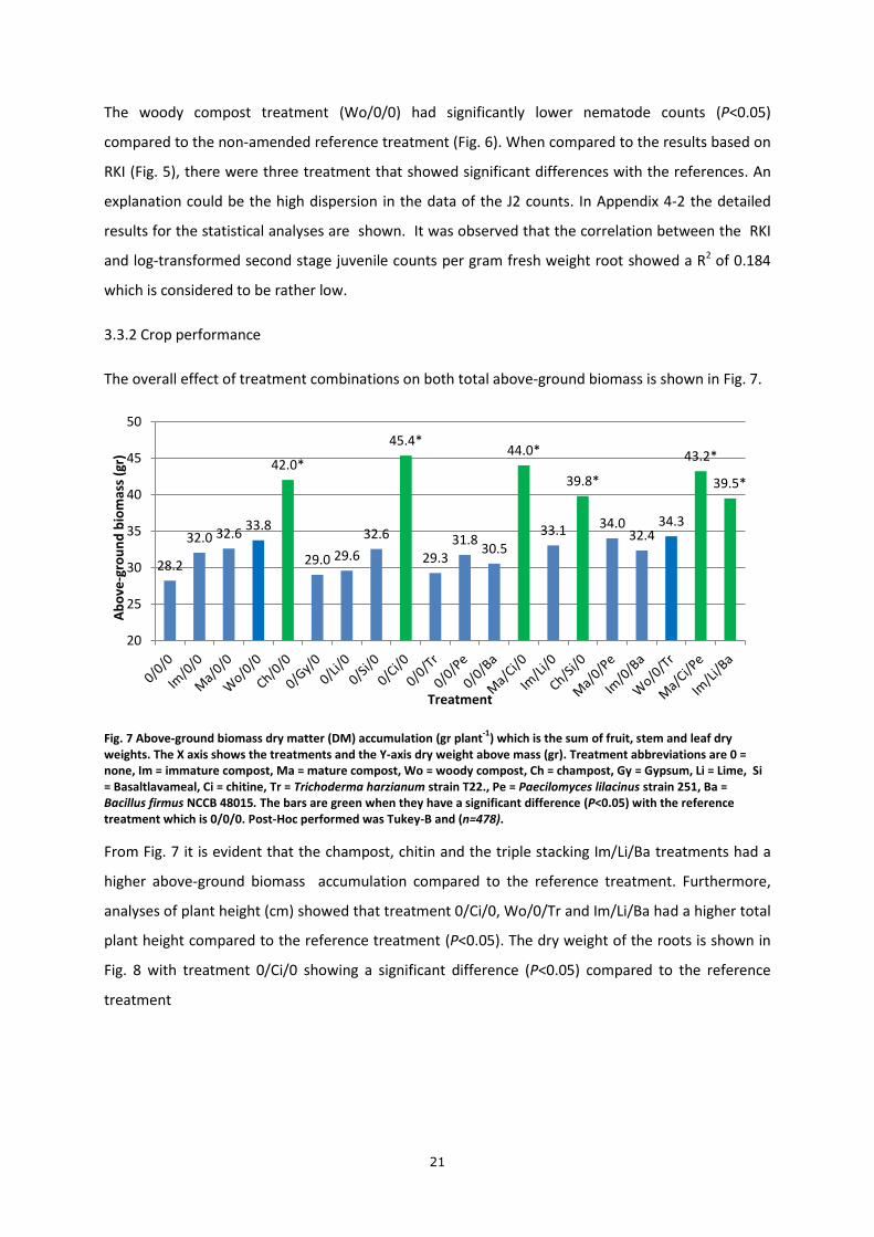
The woody compost treatment (Wo/0/0) had significantly lower nematode counts (P<0.05)

compared to the non-amended reference treatment (Fig. 6). When compared to the results based on

RKI (Fig. 5), there were three treatment that showed significant differences with the references. An

explanation could be the high dispersion in the data of the J2 counts. In Appendix 4-2 the detailed

results for the statistical analyses are shown. It was observed that the correlation between the RKI

and log-transformed second stage juvenile counts per gram fresh weight root showed a R2 of 0.184

which is considered to be rather low.

3.3.2 Crop performance

The overall effect of treatment combinations on both total above-ground biomass is shown in Fig. 7.

Fig. 7 Above-ground biomass dry matter (DM) accumulation (gr plant-1

) which is the sum of fruit, stem and leaf dry weights. The X axis shows the treatments and the Y-axis dry weight above mass (gr). Treatment abbreviations are 0 = none, Im = immature compost, Ma = mature compost, Wo = woody compost, Ch = champost, Gy = Gypsum, Li = Lime, Si = Basaltlavameal, Ci = chitine, Tr = Trichoderma harzianum strain T22., Pe = Paecilomyces lilacinus strain 251, Ba = Bacillus firmus NCCB 48015. The bars are green when they have a significant difference (P<0.05) with the reference treatment which is 0/0/0. Post-Hoc performed was Tukey-B and (n=478).

From Fig. 7 it is evident that the champost, chitin and the triple stacking Im/Li/Ba treatments had a

higher above-ground biomass accumulation compared to the reference treatment. Furthermore,

analyses of plant height (cm) showed that treatment 0/Ci/0, Wo/0/Tr and Im/Li/Ba had a higher total

plant height compared to the reference treatment (P<0.05). The dry weight of the roots is shown in

Fig. 8 with treatment 0/Ci/0 showing a significant difference (P<0.05) compared to the reference

treatment

28.2

32.0 32.6 33.8

42.0*

29.0 29.6

32.6

45.4*

29.3 31.8

30.5

44.0*

33.1

39.8*

34.0 32.4

34.3

43.2*

39.5*

20

25

30

35

40

45

50

Ab

ove

-gro

un

d b

iom

ass

(gr)

Treatment

22

Fig. 8 Dry matter (DM) root gr plant-1

. The X axis shows the treatments and the Y-axis dry weight root (gr). Treatment abbreviations are 0 = none, Im = immature compost, Ma = mature compost, Wo = woody compost, Ch = champost, Gy = Gypsum, Li = Lime, Si = Basaltlavameal, Ci = chitine, Tr = Trichoderma harzianum strain T22., Pe = Paecilomyces lilacinus strain 251, Ba = Bacillus firmus NCCB 48015. The bars are green when they have a significant difference (P<0.05) with the reference treatment which is 0/0/0. Post-Hoc performed was Tukey-B and (n=238)

3.3.3 Correlation crop growth and nematodes

To determine if above-ground total dry weight

and root dry weight were correlated, a

bivariate correlation was performed for which

the R2 value was 0.614. Which is considered to

be relatively high. In terms of this correlation it

implies that the overall shoot root ratio was

somewhat constant.

For the RKI there was also a correlation

(P<0.05) with above-ground biomass dry

weight although the value was only 0.040. For

the second stage juveniles count number his

correlation was also significant (P<0.05) while the R2 value again was low (0.087). Since both values

are considered to be low, it was thus assumed that neither RKI nor the amount of second stage

juveniles affected growth.

3.09 3.64

4.09 3.62

4.26

3.66 3.46 3.72

5.57*

3.20 3.75

3.51

4.48 4.38 4.01

4.41

3.37 3.67

4.71 5.05

0.0

1.0

2.0

3.0

4.0

5.0

6.0D

ry w

eig

ht

roo

t (g

r)

Treatment

Fig. 9 Correlation between dry weight above biomass (gr) and dry weight roots (gr) n=238

23

3.3.4 Root health

To determine if treatments affected overall root health, a visual assessment of the brown color of the

roots was made. The browning was assumed to be linked to incidence of Fusarium but this was not

validated by laboratory analysis via plating techniques. The results for the visual scoring for different

treatment combinations are shown in Fig. 10.

Fig. 10 Browning of tomato roots assumed to be linked to fusarium infection with roots being visually rated from 1= little 2=medium 3=high infection. Treatment abbreviations are 0 = none, Im = immature compost, Ma = mature compost, Wo = woody compost, Ch = champost, Gy = Gypsum, Li = Lime, Si = Basaltlavameal, Ci = chitine, Tr = Trichoderma harzianum strain T22., Pe = Paecilomyces lilacinus strain 251, Ba = Bacillus firmus NCCB 48015. The bars are green when they have a significant difference (P<0.05) with the reference treatment which is 0/0/0. Post-Hoc performed was Tukey-B and n=472.

An overview of the level of Fusarium spp. infection of the root system based on brown discoloration

of the roots systems is shown in Fig. 10 . The reference treatment had the highest score. With

exception of the Im/0/0 treatment, all compost-based treatments had significantly (P<0.05) less

browning of the roots which appears to be indicative of lower potential Fusarium spp. infection

scores compared to the reference treatment.

2.9

2.5

2.1* 2.0* 1.9*

2.4

2.5 2.5

2.3*

2.7 2.6 2.6

2.1* 2.1*

1.8* 1.8*

2.3*

1.8* 1.7*

2.2*

1

1.2

1.4

1.6

1.8

2

2.2

2.4

2.6

2.8

3

Bro

wn

ing

roo

ts 1

= lit

tle

3 =

mu

ch

Treatment

24

3.4 Results Research Question2

In this paragraph results related to Research Question 2 are being presented. The section is divided in

subsections as related to the stackings for champost-, woody compost, mature- and immature

compost-based treatment combinations.

3.4.1 Champost-based stackings

As discussed in Section 3.3, champost compost-based treatment combined with Basaltlavameal (si)

showed a significant decline in RKI, analysed of all treatments. Results in terms of effects on

nematode incidence and plant growth parameters for champost-based stacking are presented in

Table 9.

Nematode assessment

The champost and basaltlavameal stacking resulted in a synergy among main means as it caused a

significant reduction (F=4.503; P<0.05) in RKI as compared to either single means such as champost

(Ch) or Basaltlavameal (Si) application. In terms of 2nd Stage Juvenile Counts (#J2/gr FR) no synergetic

effect (P>0.05) associated with stacking of treatments was found.

Crop performance

In terms of crop growth the L-matrix analyses showed that the stacking for the above-ground dry

weight resulted in an antagonistic effect (F=4.341; P<0.05) and for dry weight roots there was no

clear stacking effect (P>0.05).

Table 9 Effects of champost-based stacking on Root Knot Index (RKI, 0-10), second stage juvenile counts per fresh weight root mass ([#J2/gr FR], shoot and root dry weight of the champost stacking. Champost (Ch) and Basaltlavameal (Si). Mean separation was based on a Tukey-B Post Hoc performed test.

RKI (0-10)

n=96 [#J2/gr FR]

n=48 Dry weight Shoot (gr)

n=96 Dry weight root (gr)

n=48 Fresh Weight Root (gr)

n=96

0/0/0 4.0bc 21.0b 28.2b 3.1a 32.1b

Ch/0/0 3.8b 6.8a 42.0a 4.3a 43.8a

0/Si/0 4.0c 25.6b 32.6b 3.7a 36.0ab

Ch/Si/0 3.5a 7.7a 39.8a 4.0a 40.9ab

25

3.4.2 Woody compost-based stackings

As discussed in Section 3.3, woody compost-based treatments showed a significant decline in RKI,

analysed of all treatments. The effect of woody compost-based stacking on nematodes and plant

growth are presented in Table 10.

Nematode assessment

Analyses with L-matrix using contrasts resulted in an antagonistic effect of the stacking of woody

compost (Wo) with T. harzianum (Tr) in terms of the RKI values (F=6.797; P<0.05). This implies that

when Tr and Wo are being used simultaneously the effect is not amplified when compared to single

means of either Tr or Wo separate. Similar effects where observed for 2nd stage juvenile densities

(F=4.386; P<0.05)

Crop performance

Based on the L-matrix analyses it also appears that there was no significant effect (P>0.05) of the

stacking on the above-ground dry matter accumulation and the dry weight of the roots (Table 10)

when compared to single means of either Tr or Wo separate.

Table 10 Means of the RKI (0-10), #J2/gr FR, dry weight of the shoot and fresh weight root of the woody stacking. Abbreviations are woody (Wo) and Trichoderma harzianum strain T22 (Tr). Post Hoc test performed was Tukey-B

RKI (0-10)

n=96 #J2/gr FR n=48

Dry weight Shoot (gr) n=96

Dry weight root (gr) n=48

0/0/0 4.0c 21.0b 28.2b 3.1a

Wo/0/0 3.4a 3.9a 33.8a 3.6a

0/0/Tr 3.9c 10.2ab 29.3b 3.2a

Wo/0/Tr 3.7b 5.8a 34.3a 3.7a

26

3.4.3 Mature compost-based stackings

The effect of mature compost-based stackings on nematodes and plant growth are presented in

Table 11. In this case there were incidences of both double (two factors) and triple (three factors).

More specifically, mature compost-based systems were compared to those stacked with either chitin

or P. lilacinus. The triple mode action (Mature compost + chitin + P. lilacinus) was compared to

either one of the double mode action (Mature compost + P. lilacinus and Mature compost and chitin)

treatments.

Table 11 Means of the RKI (0-10), #J2/gr FR, dry weight of the shoot and fresh weight root of the mature stacking. Treatment abbreviations are Mature (Ma), Chitin (Ci) and Paecilomyces lilacinus strain 251 (Pe). Post Hoc test performed was Tukey-B

RKI (0-10) #J2/gr FR Dry weight Shoot (gr) Dry weight root (gr)

n=166 n=83 n=166 n=83

0/0/0 4.0abc 21.0abc 28.2b 3.1b

Ma/0/0 4.3c 53.3cd 32.6b 4.1ab

0/Ci/0 3.8a 8.4a 45.4a 5.5a

0/0/Pe 4.2bc 27.8bcd 31.8b 3.8ab

Ma/Ci/0 4.0ab 13.1ab 44.0a 4.5ab

Ma/0/Pe 4.1bc 81.8d 34.0b 4.4ab

Ma/Ci/Pe 4.0bc 31.0bcd 43.2b 4.7ab

Nematode assessment

For the RKI there was a synergetic effect (F=6.173; P<0.05) of stacking mature compost with P.

lilacinus compared to applying P. lilacinus separate. But the RKI values were still above the reference

treatment. The #J2/gr FR count did not show any significant stacking effects (P>0.05)

Crop performance

The effect of stacking of mature compost-based with chitin on shoot dry matter accumulation was

antagonistic (F=3.928; P<0.05) since stacking mature compost + chitin resulted in lower shoot dry

weights compared to applying chitin separate. In Appendix A5.3 the statistical analyses of this

synergetic and antagonistic effects can be found. No significant (P>0.05) effects were found.

27

3.4.4 Immature compost-based stackings

The effect of immature compost-based stacking on nematodes and plant growth are presented in

Table 12. In this case there were incidences of both double (two means) and triple (three means).

More specifically, immature compost-based systems were compared to those stacked with either

lime or B. firmus. The triple mode action (Immature compost + lime + B. firmus) was compared to

either of the double mode action (Immature compost with B. firmus and Immature compost with

lime) treatments.

Table 12 Means of the RKI (0-10), #J2/gr FR, dry weight of the shoot and fresh weight root of the immature stacking. Treatment abbreviations are Immature (Ma), Lime (Li) and Bacillus firmus NCCB 48015 (Ba). Post Hoc test performed was Tukey-B

RKI (0-10) #J2/gr FR Dry weight Shoot (gr) Dry weight root (gr)

n=168 n=84 n=168 n=84

0/0/0 4.0ab 21.0a 28.2b 3.1b

Im/0/0 4.0ab 33.3a 32.0b 3.6ab

0/Li/0 4.1b 18.6a 29.6b 3.5ab

0/0/Ba 4.1b 12.0a 30.5b 3.5ab

Im/Li/0 4.0ab 13.0a 33.1b 4.4ab

Im/0/Ba 3.9ab 23.9a 32.4b 3.4ab

Im/Li/Ba 3.9a 9.1a 39.5a 5.0a

Nematode assessment

For the RKI there was a synergetic effect (F=4.020; P<0.05) of stacking immature compost with B.

firmus compared to applying B. firmus separate and for stacking immature compost with lime

compared to applying lime separate. The #J2/gr FR count did not show any significant stacking

effects (P>0.05)

Crop performance

For above-ground dry weight (gr) there was a synergetic effect (F=3.090; P<0.05) of stacking

immature compost + lime + B. firmus compared to immature compost + B. firmus while other

stacking effects were not significant (P>0.05). In Appendix A5-4 more detailed statistical analyses of

synergetic and antagonistic effects can be found.

28

4 Discussion

4.1 Research Question 1 For the statistical analysis conducted to address Research Question 1, a total of twenty treatments

were included which were outlined in Section 2.1. The woody compost-based stackings typically

reduced RKI (P<0.05) both if compost occurred as single means but also when it was stacked with T.

harzarium compared with the reference treatment. The RKI for stacking based on either champost

and basaltlavameal was also significant lower (P<0.05) compared to the reference. Similarly, for 2nd

stage juvenile per gram fresh weight root were significant (P<0.05) lower for woody compost

separate compared to unammended reference treatment.

Result thus revealed that the use of woody compost had a suppressive effect on RKN (Fig. 5 and Fig.

6). This may be attributed to the relatively high C/N ratio, lignin content and pH values of the

compost material. Research on soil suppressiveness and functional diversity of the soil microflora in

organic farming systems in the Netherlands showed that soils with i.a. a high C/N quotient favour

high populations of antagonistic Streptomyces spp. (Postma et al, 2008). Similar observations were

made for microbial communities in boreal forest soils (Hogberg et al, 2006) while there is also a

close correlation between C/N ratio and bacterial and eukaryotic community structures (Marschner

et al, 2003). Therefore, it appears that indigenous antagonistic organisms may be stimulated due to

an increase in C/N ratio of added organic amendment. Furthermore, not only the C/N ratio has effect

on the microbial community since the type of carbon content also has an influence on this

composition as well. For an example, it was shown that lignin amendments changed soil microbial

community structure (Beneden et al, 2010). For the woody material used in this research it is

supposed that it had a relatively high lignin content in comparison to the other compost types.

Another factor governing soil suppressiveness is the pH of either the soil amendment and its effect

on soil pH. The woody compost had a pH of 7.5 (Table 4) and the reference soil a pH of 6.5.

Therefore, it is assumed that there was a pH increase due to the addition of the woody compost. The

fungal to bacteria ratio in soil systems is influenced by pH (Hogberg et al, 2006). Generally it can be

said that fungal pathogens prefer lower pH while bacteria thrive better in high pH environments

(Oka, 2014).

In terms above-ground biomass production, use of woody did not enhance crop growth. This could

be explained by the higher C/N of this material which may increase the potential risk of (initial)

immobilisation of nitrogen compared to the reference treatment. However, over time it is to be

expected that that net mineralization will be relative higher compared to the reference treatment

29

due to the decomposition of the added woody compost material. Which is in agreement with the

observed results since there was no negative effect seen on growth. Another reason why growth

was not stimulated may be related to an increase of pH potentially reducing the availability and

uptake of nutrients as iron (Finck, 1976).

For the pure champost treatment it is noticeable that it had an high EC and OM%, which were shown

to have a suppressive effect on RKN (Wurff, unpublished data 2014) Furthermore, the champost had

a higher ammonium to nitrate ratio compared to the reference treatment. Research showed that use

of N materials with a higher ammonium to nitrate ratio resulted in a reduction in severity of root

knot nematodes one month after application (Spiegel et al, 1982). The measurements of the pure

champost showed a composition of 19 to 1 (N-NH4 to N-NO3). Furthermore, shoot growth was also

stimulated (P<0.05) by the champost addition compared to the reference treatment. Elaborating on

this, it may be argued that the high EC due to higher nutrient amounts, OM% and nitrogen contents

could have had a positive effect on overall plant growth. Also the addition of chitin showed an

increase in above-ground plant dry weight, which could be explained by the addition of nitrogen

within the chitin (Kumar and Majeti, 2000) whereas the extra nitrogen could promote plant growth.

In woody compost and the champost the structure of the soil may have also changed compared to

the reference treatment. Research with the migration of J2 of M. incognita showed that presence of

large macropores prevented J2 juveniles from migrating (Otobe et al, 2004). This may partially

explain why both the champost as the woody compost treatments had lower nematode densities

and scores. In this case an increase of larger sized pores due to the addition of these materials that

still contain a large percentage of rather large/crude components may have cause discontinuities in

the soil matrix which could have hampered to movement and spread of nematodes throughout the

soil matrix.

4.2 Research Question 2. For Research Question 2, four stackings were included in this research: Woody compost and

antagonist T. harzianum, champost with lava basalt meal and silicon, and immature compost with

lime and B. firmus and mature compost with chitin and P. lilacinus.

For the stacking of Woody compost with T. harzianum it was hypnotized that this would enhance the

growth of T. harzianum as suggested by various authors (Nelson et al, 1983; Hoitink and Boehm,

1999). However, based on RKI and #J2/gr FR counts there was no evidence that this treatment

combination resulted in a decline of nematodes as the RKI for this stacking did not decrease

compared to applying woody compost separate.

30

For champost treatments, a stacking with basaltlavameal resulted in a synergetic effect in terms of

reducing RKI values (which is indicative of reduced severity of nematodes infection) compared to the

usage of champost or basaltlavameal alone. The absorbability of silicon by the plants is dependent on

the structure and moisture content of the soil.

It was reported that redoxpotential (Eh) decreases as the soil water content in a Yolo silt loam

increased and anaerobic microsites start dominating the soil system . The decrease of the Eh was not

only high at high saturation levels, but at 58% to 60% of the pores filled with water Eh was already

decreased drastic. It was discussed that this effect occurred because the smaller pores where

completely filled with water and gradually became anaerobic. In this context, it is relevant to note

that microbial activity is often concentrated in micropores (Za´ rate-Valdez, 2006). Moreover, a

decrease in soil Eh could increase the solubility of soil Si (Ponnamperuma, 1965). Although structure

of the soil changed in terms of an increased number pores and less solid parts due to addition of

champost (see Table 6 and 7) no clear effects on soil moisture content could be discerned. More

detailed measurements thus are needed in future studies to determine whether more soluble Si was

available due to champost addition. Furthermore, research with transplanted rice showed that when

applying Si, the uptake of phosphorus, calcium, magnesium and the formation of carbohydrate was

increased but for nutrients as nitrogen, potassium, iron the uptake decreased (Islam and Saha, 1969)

Also ammonium acetates were used as extractant for soil Si (Sauer et al.,2006) and analysis showed

that there is a direct relation between soil nutrient composition and plant available Si.

Although synergetic effects for the RKI (P<0.05) were observed for mature compost-based stacking

with P. lilacinus compared to applying P. lilacinus alone, the RKI was not lower compared to the

reference treatment. The #J2/gr FR values for the mature compost + P. lilacinus was highest of all

treatments within the mature compost stacking. Therefore, it is evident that there was no synergistic

suppressive effect on RKN for this specific stacking combination. Furthermore, nematode counts at

the start of Phase 1 showed a higher number of thermophilic Meloidogyne nematodes in the mature

compost treatment compared to the reference treatment. However, there is no clear explanation for

the increase nematode counts due to the application of mature compost. Therefore, further

biochemical and microbial analyses of the compost material would be needed to explain potential

differences.

31

Immature compost-based stacking had no suppressive effect on RKI or #J2/gr FR values. This is in

contrast with reports in the literature were it was documented that with an increase in the

ammonium to nitrate ratio, the incidence of nematodes per mm root would decrease (Spiegel et al,

1982). However, overall nitrate values were relatively high. Moreover, it should be noted that both

immature and mature compost had a relative low organic matter content which reduces its

effectiveness as a soil amendment as related to soil structure and nematode suppressing properties.

32

5 Conclusion

Before starting this research two hypothesises were formulated. The first hypotheses was that

the use of compost, soil additives and bio-organism will enhance or maintain plant growth and

reduce the RKI and/or #J2/gr FR compared to the non-amended group. Table 13 provides an

overview of the outcomes related to the first hypotheses.

Table 13 Hypotheses acception or rejection for the RKI, #J2/gr FR, Dry weight shoot and root

Significant difference Hypotheses accepted for 1 or more

treatments

RKI Significantly lower (P<0.05) in

Wo/0/0, Ch/0/0 and Wo/0/Tr

Yes

#J2/gr FR Significantly lower (P<0.05) in woody

compost (T4)

Yes

Dry weight shoot Significantly higher (P<0.05) in

treatments Ch/0/0, Ch/Si/0, 0/Ci/0,

Ma/Ci/0, Ma/Ci/Pe and Im/Li/Ba. No

treatments where significantly lower

than the reference treatment 0/0/0.

Yes

Dry weight root Significantly higher (P<0.05) in

treatments Ch/0/0, Ch/Si/0, 0/Ci/0

Yes

As seen in Table 13, none of the treatments showed a decline in shoot or root dry weight compared

to the reference treatment. Thus all amendments sustained or even enhanced overall crop growth.

For the nematodes assessment the hypotheses for the RKI was accepted for treatment Wo/0/0,

Ch/0/0 and Wo/0/Tr while for the second stage juvenile count density the hypotheses was accepted

for Wo/0/0. Furthermore RKI had a correlation (P<0.05) with R-squared value of 0.040 with above-

ground dry weight (gr) while for second stage juvenile count density this correlation (P<0.05) with

above dry weight was this value was not much higher (R2 = 0.079). Both values are considered to be

low which may be related to regression slopes being close to zero. Therefore it is assumed that RKI

and #J2/gr FR did not have a pronounced effect on root growth.

The second hypotheses was based on the stacking of different means and was formulated as follow:

The RKI and #J2/gr FR is higher in singular or double means treatment compared to treatments that

entail a stacking of double or triple means. In Table 14 an overview of the conclusions is given.

33

Table 14 Conclusions and hypotheses acception or rejection for the effect of the stackings with immature, mature, woody and champost compost.

Stacking RKI #J2/gr FR

Immature Hypothesis accepted because stacking immature

compost with B. firmus resulted in a synergetic

effect (F=4.020; P<0.05) in terms of a lower RKI

compared to applying B. firmus separate. This

also complied (F=4.020; P<0.05) for stacking

immature compost with lime compared to

applying lime separate.

Hypothesis rejected as there was

no clear (significant) effect.

Mature Hypothesis accepted because stacking mature

compost with P. lilacinus resulted in a synergetic

effect (F=6.173, P<0.05) in terms of a lower RKI

compared to applying P. lilacinus separate.

Hypothesis rejected as there was

no clear (significant) effect.

Woody Hypothesis rejected as there was an antagonistic

effect Antagonistic effect of the stacking woody

compost with T. harzianum (F=6.797; P<0.05).

Hypothesis rejected as there was

an antagonistic effect of the

stacking woody compost with T.

harzianum (F=4.386; P<0.05)

Champost Hypothesis accepted because a synergetic effect

(F=4.503; P<0.05) of the stacking champost with

basaltlavameal was found.

Hypothesis rejected as there was

no clear (significant) effect.

As seen in Table 14 the immature, mature and champost showed one or more synergetic effects

according to the L-matrix. Although there were synergetic effect found in the immature and mature

compost-based stacking it didn’t result in a decline in RKI or #J2/gr FR. For the champost stacking the

stacking did reduce the RKI compared to applying the means separate.

34

6. Recommendations

In applied research, it is important to be as close as possible to actual practice, i.e., to mimic the

conditions of the greenhouse of organic vegetable growers. Therefore, all means where in

agreement with SKAL regulation for organic agriculture in the Netherlands. One of the aims of this

research was to translate the results to practice. However, a few difficulties arose in translating the

results to practise: This research was performed in pots whereas the organic growers grow their

vegetables in the soil. The use of pots allows for fine-tuning different environmental conditions as

moisture content and to implement many different treatments in a limited amount of space. The

duration of this research was 12 weeks whereas the cultivation of tomatoes is a year. Some of the

measures, such as woody compost, may show good results during the first two months of the

cultivation but have none or even negative effect during the rest of the growing season because for

example of decomposition of material.

The advantage of using commercially available compost is that outcome of the experiments can be

used immediately. For example, the champost is a waste product from mushroom growers, which

presents a win-win situation for mushroom- and vegetable growers. The woody compost is a fraction

of the compost that is normally sieved out to produce, immature and mature compost.

According to this research, the woody and champost compost have the highest potential for further

research. The underlying mechanism is not studied here, however, the high NH4 load might kill

nematodes in soil. Because of the relative high NH4-N/ NO3-N ratio of champost, it would be an idea

to increase the pH in combination with the addition of champost in a next research to stimulate the

conversion of NH4 to NH3. Relating to plant toxicity the threshold value of NH4 and NH3 have to be

determined to maximize RKN decline and minimize plant growth reduction. Applying champost in the

period before planting in a bare soil would have the advantage that a temporally increase in pH and

NH3 would not directly affect plant growth. Further research is also needed to determine the time

span and amount that are needed to supress RKN and prevent plant toxic effects. The amount and

time used in this research didn’t show negative effect on plant growth. Furthermore for woody

compost it would be interesting to study mechanisms behind the suppressive effect of woody

material against RKN as discussed in the discussion chapter. In this study it would be interesting to

make distinction between different types of woody material.

35

At the start of phase 1 many plants were destroyed by wood-lice (Armadillidium spp.). To prevent

this potential problem during subsequent studies, preventive addition of slug pellets may be

advisable. Frequent and careful observation especially on pest and deceases is also needed directly

after planting. In a research with RKN it is important to minimize the effect of others factors outside

the research goals. For example in this research calculations were made to prevent plant to have a

deficiency of nutrients, therefore every week measurements of NO3 in the soil of the border plants

were performed to start with fertilizing before a deficiency of NO3 would occur.

Finally, cautious is needed to use this results directly in practice since this is a preliminary study. It is

recommended to do more research on the arguments discussed in above paragraphs.

36

References

Beneden van, S., Roobroeck, D., Franta, S.C., De Neve, S., Boeckx, P., Hofte, M. 2010. Microbial

populations involved in the suppression of Rhizoctonia solani AG1-1B by lignin incorporation in soil.

Soil Biology and Biochemistry. 42: 1268–1274.

CEN European committee for standardization. 1999. Soil improvers and growing media –

Determination of physical properties, dry bulk density, air volume, water volume, shrinkage value

and total pore space. EN 13041.

Davies, L.J., Brown, C.R., Elling, A.A. 2014. Calcium is involved in the RMc1(blb)-mediated

hypersensitive response against Meloidogyne chitwoodi in potato. Plant Cell Reports 34: 167–177.

Finck, A. 1976. Pflanzenernährung in Stichworten. Kiel: Hirt. p. 80.

Gatarayiha, M. C., Laing, M. D., Miller, R. M. 2010. Combining applications of potassium silicate and

Beauveria bassiana to four crops to control two spotted spider mite, Tetranychus urticae Koch.

International Journal of Pest Management 56: 291-297.

Goswami, B.K., Singh, S., Verma, V.S. 1976. Uptake and translocation of calcium and magnesium in

tomato plants as influenced by infection with Root-knot Nematode Meloidogyne incognita and

tobacco mosaic virus. Nematologica 22: 116 – 117.

Guffanti, A. A., Blanco, R., Benenson, R. A., Krulwich, T.A. 1980. Bioenergetic Properties of Alkaline-

tolerant and Alkalophilic Strains of Bacillus firmus. Microbiology 119: 79–86.

Högberg, M.N., Högberg, P., Myrold, D.D. 2007. Is microbial community composition in boreal forest

soils determined by pH, C-to-N ratio, the trees, or all three? Oecologia 150: 590–601.

Hoitink, H.A.J., Boehm, M.J. 1999. Biocontrol within the context of soil microbial communities: a

substrate-dependent phenomenon. Annual Review of Phytopathology 37: 427–446.

Howell, G.T., Lacroix G.L. 2012. Decomposing interactions using GLM in combination with the

COMPARE, LMATRIX and MMATRIX subcommands in SPSS. Quantitative Methods for Psychology 8:

1–22.

37

Islam, A., Saha, R. 1969. Effects of silicon on the chemical composition of rice plants. Plant and Soil

30: 446-458.

Khan, A., Williams, K. L., Molloy, M. P., Nevalainen, H. K. M. 2003. Purification and characterization of

a serine protease and chitinases from Paecilomyces lilacinus and detection of chitinase activity on 2D

gels. Protein Expression and Purification 32:210-220.

Kumar, R., Majeti, N.V., 2000. A review of chitin and chitosan applications. Reactive and Functional

Polymers 46:1-27.

Ranger, C. M., Singh, A. P., Frantz, J. M., Canas, L., Locke, J. C., Reding, M. E., Vorsa, N. 2009.

Influence of Silicon on Resistance of Zinnia elegans to Myzus persicae (Hemiptera: Aphididae).

Environmental Entomology 38: 129-136.

Terefe, M., Tefera, T., Sakhuja, P.K. 2009. Effect of a formulation of Bacillus firmus on root-knot

nematode Meloidogyne incognita infestation and the growth of tomato plants in the greenhouse and

nursery. Journal of Invertebrate Pathology 100: 94–99.

Marschner, P., Kandeler, E., Marschner, B. 2003. Structure and function of the soil microbial

community in a long-term fertilizer experiment. Soil Biology and Biochemistry 35: 453–461.

Miller, J.G., Faske, T.R., 2011, Abstract of Response of Meloidogyne incognita to silicon,

Phytopathology 101: S267.

Mittal, N., Saxena, G., Mukerji, K.G. 1995. integrated control of root-knot disease in three crop plants

using chitin and Paecilomyces lilacinus. Crop Protection 14: 647-651.

Nelson, E.B., Kuter, G.A., Hoitink, H.A.J. 1983. Effects of fungal antagonists and compost age on

suppression of Rhizoctonia damping-off in container media amended with composted hardwood

bark. Phytopathology, 73: 1457–1462.

Oka, Y., Tkachi, N., Shuker, S., Rosenberg, R., Suriano, S., Fine, P. 2006. Field studies on the

enhancement of nematicidal activity of ammonia-releasing fertilisers by alkaline amendments.

Nematology 8: 881–893.

38

Oostenbrink, M. 1960. Estimating nematode populations by some selected methods. In Nematology

eds. Sasser, J.N., Jenkins,W.R. pp. 85–102. The University of North Carolina Press, Chapel Hill.

Otobe, K., Itou, K., Mizukubo, T. 2004. Micro-moulded substrates for the analysis of structure-

dependent behaviour of nematodes. Nematology 6: 73-77.

Oteifa, B.A. 1955. Nitrogen source of the host nutrition in relation to infection by a root knot

nematode, Meloidogyne incognita. Plant Disease Reporter 39: 902-903.

Ponnamperuma, F.N. 1965. Dynamic aspects of flooded soils and the nutrition of the rice plant. The

Mineral Nutrition of the Rice Plant: 295-328.

Postma, J., Schilder, M. T., Bloem, J., Leeumen-Haagsma van, W.K. 2008. Soil suppressiveness and

functional diversity of the soil microflora in organic farming systems. Soil Biology Biochemistry 40:

2394-2406.

Sauer, D., Soccone, L., Conley, D.J., Hermann, L., Sommer, M. 2006. Review of methodologies for

extracting plant available and amorphous Si from soils and aquatic sediments. Biogeochemistry 80:

89-108.

Sharon, E., Bar-Eyal, M., Chet, I., Herrera-Estrella, A., Kleifeld, O., Spiegel, Y. 2001. Biological control

of the root-knot nematode Meloidogyne javanica by Trichoderma harzianum. Phytopathology 91:

687–693.

Sonneveld, C. 1990. Estimating quantities of water-soluble nutrients in soil using a specific 1:2

volume extract. Communications in Soil Science and Plant Analyses 21: 1257–1265.

Sonneveld, C., Voogt, W. 2009. Plant nutrition of greenhouse crops. Springer Dordrecht Heidelberg

London New York. 431 pp.

Spiegel, Y., Chet, I., Cohn, E., Galper, S., Sharon, E., 1988, Use of chitin for controlling plant-parasitic

nematodes. Plant and Soil 109: 251-256.

Spiegel, Y., Cohn, E., Kafkaki, U. 1982. The influence of ammonium and nitrate nutrition of tomato

plants on parasitism by root-knot nematode. Phytoparasitica 10: 33-40.

39

Stone, A.G., Traina, S.J., Hoitink, H.A.J. 2001. Particulate Organic Matter Composition and Pythium

Damping-Off of Cucumber. Soil Science Society of America Journal 65:761-770.

Suarez, B., Rey, M., Castillo, P. 2004. Isolation and characterization of PRA1, a trypsin-like protease

from the biocontrol agent Trichoderma harzianum CECT 2413 displaying nematicidal activity. Applied

Microbiology and Biotechnology 65: 46–55.

Wurff1 van der, A.W.G., Janse1, J., Kok2, C.J., Zoon2, F.C. 2010. Biological control of root knot

nematodes in organic vegetable and flower greenhouse cultivation. 1Wageningen UR Glastuinbouw,

Bleiswijk. 2Plant Research International, Wageningen. Wageningen UR Glastuinbouw. Report 321.

Za´ rate-Valdez, J.L., Zasoski, R.J., La’ uchli, A.E., 2006, Short-term effects of moisture content on soil

solution pH and soil Eh. Soil Science 171: 5.

Zhang, L.H., Mojtahedi , H., Kuang, H., Baker, B., and Brown, C.R. 2007. Marker-assisted selection of

Columbia root-knot nematode resistance introgressed from Solanum bulbocastanum. Crop Science

47: 2021–2026 .

Websites and others

1. http://dictionary.reference.com/browse/synergy

2. Konica Minolta. 2009. Manual Chlorophyll meter SPAD 502 Plus

3. Oka, Y. 2014., personal communication

4. Wurff van der, A.W.G. 2014. Unpublished data

5. Wurff van der, A.W.G. 2014. PPS, werkplan duurzame bodem kasteelt. TKI number KV1309

084

40

Appendices

Appendix A1 Score chart used to determine Root Knot Index (RKI) 1 values

1 Source: Wurff1 van der, A.W.G., Janse1, J., Kok2, C.J., Zoon2, F.C. 2010. Biological control of root knot

nematodes in organic vegetable and flower greenhouse cultivation. 1Wageningen UR Glastuinbouw,

Bleiswijk. 2Plant Research International, Wageningen. Wageningen UR Glastuinbouw. Report 321.

41

Appendix A2 Experimental map layout

42

Appendix A3-1 Temperature and radiations levels in the greenhouse.

The next figures show the realized temperature and artificial lightning during the research.

Fig. 11 temperature °C realization during the total research period of phase 1 and 2. At -12 DAP the transplants were placed in the greenhouse and therefore temperature heating set point was set to 20/20 °C Day/Night

Fig. 12 artificial lighting realization during the total research period of phase 1 and 2. Values given are average values in PAR µmol/m

-2/s

-1

As seen in Fig. 11 the temperature realized from -33 dap till -12 dap is colder compared to the period

from -12 DAP till 57 DAP. In this cold period a biological equilibrium was meant to be set without

losing to many nematodes in the soil, because the life cycle period of the RKN is temperature

dependent. For the artificial lighting the length of lighting per day was dependent on the outside

radiation.

0

5

10

15

20

25

-33

-29

-25

-21

-17

-13 -9 -5 -1 3 7

11

15

19

23

27

31

35

39

43

47

51

55

Tem

per

atu

re °

C

DAP

0

20

40

60

80

100

120

-33

-29

-25

-21

-17

-13 -9 -5 -1 3 7

11

15

19

23

27

31

35

39

43

47

51

55

Avg

PA

R µ

mo

l/m

-2/s

-1

DAP

43

Appendix A3-2 Irrigation realization

February March

DAP Day Watering per plant (ml) DAP Day Watering per plant (ml)

13 1 220 41 1 400

14 2 150 42 2 150

15 3 100 43 3 340

16 4 100 44 4 300

17 5 100 45 5 350

18 6 100 46 6 300

19 7 50 47 7 300

20 8 50 48 8 300

21 9 100 49 9 300

22 10 50 50 10 300

23 11 50 51 11 350

24 12 50 52 12 350

25 13 50* 53 13 350

26 14 140 54 14 300

27 15 100 55 15 250

28 16 50

29 17 100

30 18 100

31 19 100

32 20 100

33 21 180

34 22 120

35 23 100

36 24 300

37 25 250*

38 26 100

39 27 300*

40 28 No data * extra watering was performed which differed per plant depending on the plant needs determined by the weight of the pot.

** From < DAP 13 no data is registered

44

Appendix A4 Overall statistical analyses

Appendix A4-1 RKI

Between-Subjects Factors

Name Value Label N

1,00 0/0/0 24

2,00 Im/0/0 24

3,00 Ma/0/0 24

4,00 Wo/0/0 24

5,00 Ch/0/0 24

6,00 0/Gy/0 24

7,00 0/Li/0 24

8,00 0/Si/0 24

9,00 0/Ci/0 24

10,00 0/0/Tr 24

11,00 0/0/Pe 23

12,00 0/0/Ba 24

13,00 Ma/Ci/0 23

14,00 Im/Li/0 24

15,00 Ch/Si/0 24

16,00 Ma/0/Pe 24

17,00 Im/0/Ba 24

18,00 Wo/0/Tr 24

19,00 Ma/Ci/Pe 24

20,00 Im/Li/Ba 24

Repeatment N

1 60

2 59

3 60

4 60

5 60

6 60

7 59

8 60

45

Tests of Between-Subjects Effects

Dependent Variable:

Source

Type III Sum of

Squares df

Mean

Square F Sig.

Intercept Hypothesis 7409.926 1 7409.926

20098.72

8 .000

Error 2.581 7.000 ,369a

Name Hypothesis 22.214 19 1.169 9.892 .000

Error 53.305 451 ,118b

Repeatmen

t

Hypothesis 2.581 7 .369 3.119 .003

Error 53.305 451 ,118b

a. 1,000 MS(Repeatment) + 3,831E-5 MS(Error)

b. MS(Error)

Expected Mean Squaresa,b

Source

Variance Component

Var(Repeatme

nt) Var(Error)

Quadratic

Term

Intercept 59.737 1.000

Intercept,

Name

Name 0.000 1.000 Name

Repeatment 59.739 1.000

Error 0.000 1.000

a. For each source, the expected mean square equals the sum of the

coefficients in the cells times the variance components, plus a quadratic

term involving effects in the Quadratic Term cell.

b. Expected Mean Squares are based on the Type III Sums of Squares.

46

RKI

Tukey Ba,b,c

Name N

Subset

1 2 3 4 5 6 7

Wo/0/0 24 3.3750

Ch/Si/0 24 3.5417 3.5417

Wo/0/Tr 24 3.6667 3.6667 3.6667

0/Ci/0 24 3.7500 3.7500 3.7500

Ch/0/0 24 3.7917 3.7917 3.7917 3.7917

Im/Li/Ba 24 3.8750 3.8750 3.8750 3.8750

Im/0/Ba 24 3.9167 3.9167 3.9167 3.9167 3.9167

0/0/Tr 24 3.9167 3.9167 3.9167 3.9167 3.9167

Ma/Ci/0 23 3.9565 3.9565 3.9565 3.9565 3.9565

Im/Li/0 24 3.9583 3.9583 3.9583 3.9583 3.9583

0/0/0 24 4.0000 4.0000 4.0000 4.0000

Im/0/0 24 4.0417 4.0417 4.0417 4.0417

0/Si/0 24 4.0417 4.0417 4.0417 4.0417

Ma/Ci/Pe 24 4.0417 4.0417 4.0417 4.0417

0/0/Ba 24 4.0833 4.0833 4.0833 4.0833

Ma/0/Pe 24 4.0833 4.0833 4.0833 4.0833

0/Li/0 24 4.1250 4.1250 4.1250

0/Gy/0 24 4.1667 4.1667

0/0/Pe 23 4.1739 4.1739

Ma/0/0 24 4.2500

Means for groups in homogeneous subsets are displayed. Based on observed means. The error term is Mean Square(Error) = ,118. a. Uses Harmonic Mean Sample Size = 23,896.

b. The group sizes are unequal. The harmonic mean of the group sizes is used. Type I error levels are not guaranteed. c. Alpha = 0.05.

47

Appendix A4-2 Natural logarithm number of juveniles per gram fresh weight root

Between-Subjects Factors

Value Label N

Name 1,00

0/0/0 12

2,00 Im/0/0 12

3,00 Ma/0/0 12

4,00 Wo/0/0 12

5,00 Ch/0/0 12

6,00 0/Gy/0 12

7,00 0/Li/0 12

8,00 0/Si/0 12

9,00 0/Ci/0 12

10,00 0/0/Tr 12

11,00 0/0/Pe 12

12,00 0/0/Ba 12

13,00 Ma/Ci/0 11

14,00 Im/Li/0 12

15,00 Ch/Si/0 12

16,00 Ma/0/Pe 12

17,00 Im/0/Ba 12

18,00 Wo/0/Tr 12

19,00 Ma/Ci/Pe 12

20,00 Im/Li/Ba 12

Repeatment 1 40

2 20

3 40

4 20

5 40

6 20

7 39

8 20

48

Tests of Between-Subjects Effects

Dependent Variable:

Source

Type III Sum of Squares df

Mean Square F Sig.

Intercept Hypothesis 2652.009 1 2652.009 660.327 .000

Error 29.485 7.342 4,016a

Name Hypothesis 142.874 19 7.520 7.556 .000

Error 210.983 212 ,995b

Repeatment Hypothesis 30.334 7 4.333 4.354 .000

Error 210.983 212 ,995b

a. ,905 MS(Repeatment) + ,095 MS(Error)

b. MS(Error)

Expected Mean Squaresa,b

Source

Variance Component

Var(Repeatment) Var(Error) Quadratic

Term

Intercept 26.605 1.000

Intercept, Name

Name 0.000 1.000 Name

Repeatment 29.398 1.000

Error 0.000 1.000

a. For each source, the expected mean square equals the sum of the coefficients in the cells times the variance components, plus a quadratic term involving effects in the Quadratic Term cell.

b. Expected Mean Squares are based on the Type III Sums of Squares.

49

Ln_J2_gr_root

Tukey Ba,b,c

Name N

Subset

1 2 3 4 5 6 7

Wo/0/0 12 2.1676

Wo/0/Tr 12 2.5267 2.5267

Ch/0/0 12 2.6748 2.6748 2.6748

Ch/Si/0 12 2.7981 2.7981 2.7981 2.7981

0/Ci/0 12 2.8785 2.8785 2.8785 2.8785

Im/Li/Ba 12 2.9508 2.9508 2.9508 2.9508

0/0/Tr 12 3.0610 3.0610 3.0610 3.0610

0/0/Ba 12 3.2154 3.2154 3.2154 3.2154

Im/Li/0 12 3.2934 3.2934 3.2934 3.2934 3.2934

Ma/Ci/0 11 3.3003 3.3003 3.3003 3.3003 3.3003

0/Li/0 12 3.6405 3.6405 3.6405 3.6405 3.6405

0/0/0 12 3.7628 3.7628 3.7628 3.7628 3.7628 3.7628

Im/0/Ba 12 3.8873 3.8873 3.8873 3.8873 3.8873 3.8873

0/Si/0 12 3.9542 3.9542 3.9542 3.9542 3.9542

0/0/Pe 12 4.0359 4.0359 4.0359 4.0359 4.0359

Ma/Ci/Pe 12 4.1429 4.1429 4.1429 4.1429

Im/0/0 12 4.2141 4.2141 4.2141 4.2141

Ma/0/0 12 4.6781 4.6781 4.6781

0/Gy/0 12 4.6927 4.6927

Ma/0/Pe 12 5.1038

Means for groups in homogeneous subsets are displayed. Based on observed means. The error term is Mean Square(Error) = ,995. a. Uses Harmonic Mean Sample Size = 11,946.

b. The group sizes are unequal. The harmonic mean of the group sizes is used. Type I error levels are not guaranteed. c. Alpha = 0.05.

50

Appendix A4-3 Above dry weight (gr)

Between-Subjects Factors

Value Label N

Name 1,00 0/0/0 24

2,00 Im/0/0 24

3,00 Ma/0/0 24

4,00 Wo/0/0 24

5,00 Ch/0/0 24

6,00 0/Gy/0 24

7,00 0/Li/0 24

8,00 0/Si/0 24

9,00 0/Ci/0 24

10,00 0/0/Tr 24

11,00 0/0/Pe 23

12,00 0/0/Ba 24

13,00 Ma/Ci/0 23

14,00 Im/Li/0 24

15,00 Ch/Si/0 24

16,00 Ma/0/Pe 24

17,00 Im/0/Ba 24

18,00 Wo/0/Tr 24

19,00 Ma/Ci/Pe 24

20,00 Im/Li/Ba 24

Repeatment 1 60

2 59

3 60

4 60

5 60

6 60

7 59

8 60

51

Tests of Between-Subjects Effects

Dependent Variable:

Source Type III Sum of Squares df

Mean Square F Sig.

Intercept Hypothesis 580795.617 1 580795.617 795.894 .000

Error 5108.210 7.000 729,740a

Repeatment Hypothesis 5108.364 7 729.766 13.967 .000

Error 23563.777 451 52,248b

Name Hypothesis 13189.850 19 694.203 13.287 .000

Error 23563.777 451 52,248b

a. 1,000 MS(Repeatment) + 3,831E-5 MS(Error)

b. MS(Error)

Expected Mean Squaresa,b

Source

Variance Component

Var(Repeatment) Var(Error) Quadratic

Term Intercept

59.737 1.000 Intercept, Name

Repeatment 59.739 1.000

Name 0.000 1.000 Name Error 0.000 1.000 a. For each source, the expected mean square equals the sum of the coefficients in the cells times the variance components, plus a quadratic term involving effects in the Quadratic Term cell. b. Expected Mean Squares are based on the Type III Sums of Squares.

52

Total_dry_weight_above_gr

Tukey Ba,b,c

Name N

Subset

1 2 3 4

0/0/0 24 28.2273

0/Gy/0 24 29.0338

0/0/Tr 24 29.2733

0/Li/0 24 29.5933

0/0/Ba 24 30.5471

0/0/Pe 23 31.7600

Im/0/0 24 32.0421

Im/0/Ba 24 32.3692

0/Si/0 24 32.5600

Ma/0/0 24 32.6254

Im/Li/0 24 33.0600 33.0600

Wo/0/0 24 33.7613 33.7613 33.7613

Ma/0/Pe 24 34.0355 34.0355 34.0355

Wo/0/Tr 24 34.3008 34.3008 34.3008

Im/Li/Ba 24 39.5121 39.5121 39.5121

Ch/Si/0 24 39.8213 39.8213

Ch/0/0 24 42.0388

Ma/Ci/Pe 24 43.2279

Ma/Ci/0 23 44.0288

0/Ci/0 24 45.3675

Means for groups in homogeneous subsets are displayed. Based on observed means. The error term is Mean Square(Error) = 52,248. a. Uses Harmonic Mean Sample Size = 23,896.

b. The group sizes are unequal. The harmonic mean of the group sizes is used. Type I error levels are not guaranteed. c. Alpha = 0.05.

53

Appendix A4-4 Dry weight roots (gr)

Between-Subjects Factors

Value Label N

Name 1,00

0/0/0 12

2,00 Im/0/0 12

3,00 Ma/0/0 12

4,00 Wo/0/0 12

5,00 Ch/0/0 12

6,00 0/Gy/0 12

7,00 0/Li/0 12

8,00 0/Si/0 12

9,00 0/Ci/0 12

10,00 0/0/Tr 12

11,00 0/0/Pe 11

12,00 0/0/Ba 12

13,00 Ma/Ci/0 12

14,00 Im/Li/0 12

15,00 Ch/Si/0 12

16,00 Ma/0/Pe 12

17,00 Im/0/Ba 11

18,00 Wo/0/Tr 12

19,00 Ma/Ci/Pe 12

20,00 Im/Li/Ba 12

Repeatment 1 20

2 39

3 20

4 40

5 20

6 40

7 20

8 39

54

Tests of Between-Subjects Effects

Dependent Variable:

Source

Type III Sum of Squares df

Mean Square F Sig.

Intercept Hypothesis 3580.181 1 3580.181 113.803 .000

Error 223.210 7.095 31,460a

Name Hypothesis 93.992 19 4.947 2.179 .004

Error 479.069 211 2,270b

Repeatment Hypothesis 241.224 7 34.461 15.178 .000

Error 479.069 211 2,270b

a. ,907 MS(Repeatment) + ,093 MS(Error)

b. MS(Error)

Expected Mean Squaresa,b

Source

Variance Component

Var(Repeatment) Var(Error) Quadratic

Term

Intercept 26.544 1.000

Intercept, Name

Name 0.000 1.000 Name

Repeatment 29.273 1.000

Error 0.000 1.000

a. For each source, the expected mean square equals the sum of the coefficients in the cells times the variance components, plus a quadratic term involving effects in the Quadratic Term cell.

b. Expected Mean Squares are based on the Type III Sums of Squares.

55

Dry_weight_root_gr

Tukey Ba,b,c

Name N

Subset

1 2

0/0/0 12 3.0858

0/0/Tr 12 3.2000

Im/0/Ba 11 3.3655

0/Li/0 12 3.4617 3.4617

0/0/Ba 12 3.5058 3.5058

Wo/0/0 12 3.6242 3.6242

Im/0/0 12 3.6383 3.6383

0/Gy/0 12 3.6633 3.6633

Wo/0/Tr 12 3.6742 3.6742

0/Si/0 12 3.7217 3.7217

0/0/Pe 11 3.7527 3.7527

Ch/Si/0 12 4.0067 4.0067

Ma/0/0 12 4.0908 4.0908

Ch/0/0 12 4.2583 4.2583

Im/Li/0 12 4.3833 4.3833

Ma/0/Pe 12 4.4067 4.4067

Ma/Ci/0 12 4.4800 4.4800

Ma/Ci/Pe 12 4.7092 4.7092

Im/Li/Ba 12 5.0475 5.0475

0/Ci/0 12 5.5717

Means for groups in homogeneous subsets are displayed. Based on observed means. The error term is Mean Square(Error) = 2,270. a. Uses Harmonic Mean Sample Size = 11,892. b. The group sizes are unequal. The harmonic mean of the group sizes is used. Type I error levels are not guaranteed. c. Alpha = 0.05.

56

Appendix A4-5 Length (cm)

Between-Subjects Factors

Value Label N

Name 1,00 0/0/0 24

2,00 Im/0/0 24

3,00 Ma/0/0 24

4,00 Wo/0/0 24

5,00 Ch/0/0 24

6,00 0/Gy/0 24

7,00 0/Li/0 24

8,00 0/Si/0 24

9,00 0/Ci/0 24

10,00 0/0/Tr 24

11,00 0/0/Pe 23

12,00 0/0/Ba 24

13,00 Ma/Ci/0 23

14,00 Im/Li/0 24

15,00 Ch/Si/0 24

16,00 Ma/0/Pe 24

17,00 Im/0/Ba 24

18,00 Wo/0/Tr 24

19,00 Ma/Ci/Pe 24

20,00 Im/Li/Ba 24

Repeatment 1 60

2 59

3 60

4 60

5 60

6 60

7 59

8 60

57

Tests of Between-Subjects Effects

Dependent Variable:

Source Type III Sum of Squares df

Mean Square F Sig.

Intercept Hypothesis 8096163.705 1 8096163.705 15054.190 .000

Error 3764.681 7.000 537,801a

Name Hypothesis 7411.615 19 390.085 2.928 .000

Error 60086.945 451 133,230b

Repeatment Hypothesis 3764.718 7 537.817 4.037 .000

Error 60086.945 451 133,230b

a. 1,000 MS(Repeatment) + 3,831E-5 MS(Error)

b. MS(Error)

Expected Mean Squaresa,b

Source

Variance Component

Var(Repeatment) Var(Error) Quadratic

Term Intercept

59.737 1.000 Intercept, Name

Name 0.000 1.000 Name Repeatment

59.739 1.000

Error 0.000 1.000 a. For each source, the expected mean square equals the sum of the coefficients in the cells times the variance components, plus a quadratic term involving effects in the Quadratic Term cell. b. Expected Mean Squares are based on the Type III Sums of Squares.

58

Length_cm

Tukey Ba,b,c

Name N

Subset

1 2 3 4

0/0/0 24 122.1125

0/0/Tr 24 124.4792 124.4792

0/0/Pe 23 126.3826 126.3826 126.3826

0/0/Ba 24 126.7667 126.7667 126.7667 126.7667

Ma/0/Pe 24 127.8946 127.8946 127.8946 127.8946

Ma/0/0 24 128.1792 128.1792 128.1792 128.1792

Im/Li/0 24 128.3333 128.3333 128.3333 128.3333

Im/0/0 24 128.9292 128.9292 128.9292 128.9292

Im/0/Ba 24 129.3792 129.3792 129.3792 129.3792

0/Li/0 24 129.4792 129.4792 129.4792 129.4792

Ch/Si/0 24 130.4125 130.4125 130.4125 130.4125

0/Gy/0 24 130.4458 130.4458 130.4458 130.4458

0/Si/0 24 130.7667 130.7667 130.7667 130.7667

Ch/0/0 24 131.2083 131.2083 131.2083 131.2083

Ma/Ci/0 23 131.3696 131.3696 131.3696 131.3696

Ma/Ci/Pe 24 131.5417 131.5417 131.5417 131.5417

Wo/0/0 24 133.2708 133.2708 133.2708 133.2708

Wo/0/Tr 24 135.7458 135.7458 135.7458

0/Ci/0 24 137.8708 137.8708

Im/Li/Ba 24 138.3458

Means for groups in homogeneous subsets are displayed. Based on observed means. The error term is Mean Square(Error) = 133,230. a. Uses Harmonic Mean Sample Size = 23,896.

b. The group sizes are unequal. The harmonic mean of the group sizes is used. Type I error levels are not guaranteed. c. Alpha = 0.05.

59

Appendix A4-6 Browning roots

Between-Subjects Factors

Value Label N

Name 1,00 0/0/0 24

2,00 Im/0/0 24

3,00 Ma/0/0 21

4,00 Wo/0/0 24

5,00 Ch/0/0 24

6,00 0/Gy/0 24

7,00 0/Li/0 24

8,00 0/Si/0 24

9,00 0/Ci/0 24

10,00 0/0/Tr 24

11,00 0/0/Pe 23

12,00 0/0/Ba 21

13,00 Ma/Ci/0 23

14,00 Im/Li/0 24

15,00 Ch/Si/0 24

16,00 Ma/0/Pe 24

17,00 Im/0/Ba 24

18,00 Wo/0/Tr 24

19,00 Ma/Ci/Pe 24

20,00 Im/Li/Ba 24

Repeatment 1 60

2 59

3 60

4 54

5 60

6 60

7 59

8 60

60

Tests of Between-Subjects Effects

Dependent Variable:

Source

Type III Sum of Squares df

Mean Square F Sig.

Intercept Hypothesis 2352.169 1 2352.169 423.755 .000

Error 38.861 7.001 5,551a

Repeatment Hypothesis 38.897 7 5.557 17.190 .000

Error 143.843 445 ,323b

Name Hypothesis 53.431 19 2.812 8.700 .000

Error 143.843 445 ,323b

a. ,999 MS(Repeatment) + ,001 MS(Error)

b. MS(Error)

Expected Mean Squaresa,b

Source

Variance Component

Var(Repeatment) Var(Error) Quadratic

Term Intercept

58.815 1.000 Intercept, Name

Repeatment 58.882 1.000

Name 0.000 1.000 Name Error 0.000 1.000 a. For each source, the expected mean square equals the sum of the coefficients in the cells times the variance components, plus a quadratic term involving effects in the Quadratic Term cell. b. Expected Mean Squares are based on the Type III Sums of Squares.

61

Browning_roots_1little_3much

Tukey Ba,b,c

Name N

Subset

1 2 3 4 5 6

Ma/Ci/Pe 24 1.7083

Ma/0/Pe 24 1.7917

Wo/0/Tr 24 1.7917

Ch/Si/0 24 1.8333 1.8333

Ch/0/0 24 1.9167 1.9167

Wo/0/0 24 1.9583 1.9583 1.9583

Im/Li/0 24 2.0833 2.0833 2.0833 2.0833

Ma/Ci/0 23 2.0870 2.0870 2.0870 2.0870

Ma/0/0 21 2.0952 2.0952 2.0952 2.0952

Im/Li/Ba 24 2.2083 2.2083 2.2083 2.2083 2.2083

0/Ci/0 24 2.2500 2.2500 2.2500 2.2500 2.2500

Im/0/Ba 24 2.2500 2.2500 2.2500 2.2500 2.2500

0/Gy/0 24 2.3750 2.3750 2.3750 2.3750 2.3750

Im/0/0 24 2.5000 2.5000 2.5000 2.5000

0/Si/0 24 2.5417 2.5417 2.5417

0/Li/0 24 2.5417 2.5417 2.5417

0/0/Pe 23 2.5652 2.5652 2.5652

0/0/Ba 21 2.6190 2.6190 2.6190

0/0/Tr 24 2.6667 2.6667

0/0/0 24 2.9167

Means for groups in homogeneous subsets are displayed. Based on observed means. The error term is Mean Square(Error) = ,323. a. Uses Harmonic Mean Sample Size = 23,561.

b. The group sizes are unequal. The harmonic mean of the group sizes is used. Type I error levels are not guaranteed. c. Alpha = 0.05.

62

Appendix A5 Statistical analyses stackings

Appendix A5-1 Champost stacking

Natural logarithm J2 per gram fresh weight root

Between-

Subjects

Factors

Value Label N

Name 1,00

0/0/0 12

5,00 Ch/0/0 12

8,00 0/Si/0 12

15,00 Ch/Si/0 12

Repeatment 1 8

2 4

3 8

4 4

5 8

6 4

7 8

8 4

Tests of Between-Subjects Effects

Dependent Variable:

Source

Type III Sum of

Squares df Mean

Square F Sig.

Intercept Hypothesis 444.678 1 444.678 204.348 .000

Error 16.300 7.490 2,176a

Name Hypothesis 15.419 3 5.140 6.845 .001

Error 27.784 37 ,751

b

Repeatment Hypothesis 16.301 7 2.329 3.101 .011

Error 27.784 37 ,751

b

a. ,903 MS(Repeatment) + ,097 MS(Error)

b. MS(Error)

63

Expected Mean Squaresa,b

Source

Variance Component

Var(Repeatment) Var(Error) Quadratic

Term

Intercept 5.333 1.000

Intercept, Name

Name 0.000 1.000 Name

Repeatment 5.905 1.000

Error 0.000 1.000

a. For each source, the expected mean square equals the sum of the coefficients in the cells times the variance components, plus a quadratic term involving effects in the Quadratic Term cell. b. Expected Mean Squares are based on the Type III Sums of Squares.

Ln_J2_gr_root

Tukey Ba,b

Name N

Subset

1 2

Ch/0/0 12 2.6748

Ch/Si/0 12 2.7981

0/0/0 12 3.7628

0/Si/0 12 3.9542

Means for groups in homogeneous subsets are displayed. Based on observed means. The error term is Mean Square(Error) = ,751. a. Uses Harmonic Mean Sample Size = 12,000. b. Alpha = 0.05.

64

RKI

Between-Subjects Factors

Value Label N

Name 1,00 0/0/0 24

5,00 Ch/0/0 24

8,00 0/Si/0 24

15,00 Ch/Si/0 24

Repeatment 1 12

2 12

3 12

4 12

5 12

6 12

7 12

8 12

Tests of Between-Subjects Effects

Dependent Variable:

Source

Type III Sum of Squares df

Mean Square F Sig.

Intercept Hypothesis 1418.344 1 1418.344 8009.471 .000

Error 1.240 7 ,177a

Name Hypothesis 3.781 3 1.260 11.119 .000

Error 9.635 85 ,113b

Repeatment Hypothesis 1.240 7 .177 1.562 .158

Error 9.635 85 ,113b

a. MS(Repeatment)

b. MS(Error)

65

Expected Mean Squaresa,b

Source

Variance Component

Var(Repeatment) Var(Error) Quadratic

Term

Intercept 12.000 1.000

Intercept, Name

Name 0.000 1.000 Name

Repeatment 12.000 1.000

Error 0.000 1.000

a. For each source, the expected mean square equals the sum of the coefficients in the cells times the variance components, plus a quadratic term involving effects in the Quadratic Term cell. b. Expected Mean Squares are based on the Type III Sums of Squares.

RKI

Tukey Ba,b

Name N

Subset

1 2 3

Ch/Si/0 24 3.5417

Ch/0/0 24 3.7917

0/0/0 24 4.0000 4.0000

0/Si/0 24 4.0417

Means for groups in homogeneous subsets are displayed. Based on observed means. The error term is Mean Square(Error) = ,113. a. Uses Harmonic Mean Sample Size = 24,000.

b. Alpha = 0.05.

66

Dry weight above (gr)

Between-Subjects Factors

Value Label N

Name 1,00 0/0/0 24

5,00 Ch/0/0 24

8,00 0/Si/0 24

15,00 Ch/Si/0 24

Repeatment 1 12

2 12

3 12

4 12

5 12

6 12

7 12

8 12

Tests of Between-Subjects Effects

Dependent Variable:

Source

Type III Sum of

Squares df Mean

Square F Sig.

Intercept Hypothesis 122089.428 1 122089.428 1046.429 .000

Error 816.707 7 116,672a

Name Hypothesis 2948.645 3 982.882 16.573 .000

Error 5041.157 85 59,308b

Repeatment Hypothesis 816.707 7 116.672 1.967 .069

Error 5041.157 85 59,308b

a. MS(Repeatment)

b. MS(Error)

67

Expected Mean Squaresa,b

Source

Variance Component

Var(Repeatment) Var(Error) Quadratic

Term

Intercept 12.000 1.000

Intercept, Name

Name 0.000 1.000 Name

Repeatment 12.000 1.000

Error 0.000 1.000

a. For each source, the expected mean square equals the sum of the coefficients in the cells times the variance components, plus a quadratic term involving effects in the Quadratic Term cell. b. Expected Mean Squares are based on the Type III Sums of Squares.

Total_dry_weight_above_gr

Tukey Ba,b

Name N

Subset

1 2

0/0/0 24 28.2273

0/Si/0 24 32.5600

Ch/Si/0 24 39.8213

Ch/0/0 24 42.0388

Means for groups in homogeneous subsets are displayed. Based on observed means. The error term is Mean Square(Error) = 59,308. a. Uses Harmonic Mean Sample Size = 24,000. b. Alpha = 0.05.

68

Dry weight roots (gr)

Between-Subjects Factors

Value Label N

Name 1,00

0/0/0 12

5,00 Ch/0/0 12

8,00 0/Si/0 12

15,00 Ch/Si/0 12

Repeatment 1 4

2 8

3 4

4 8

5 4

6 8

7 4

8 8

Tests of Between-Subjects Effects

Dependent Variable:

Source

Type III Sum of Squares df

Mean Square F Sig.

Intercept Hypothesis 629.043 1 629.043 179.863 .000

Error 28.133 8.044 3,497a

Name Hypothesis 9.179 3 3.060 1.252 .305

Error 90.415 37 2,444b

Repeatment Hypothesis 25.272 7 3.610 1.477 .206

Error 90.415 37 2,444

b

a. ,903 MS(Repeatment) + ,097 MS(Error)

b. MS(Error)

69

Expected Mean Squaresa,b

Source

Variance Component

Var(Repeatment) Var(Error) Quadratic

Term

Intercept 5.333 1.000

Intercept, Name

Name 0.000 1.000 Name

Repeatment 5.905 1.000

Error 0.000 1.000

a. For each source, the expected mean square equals the sum of the coefficients in the cells times the variance components, plus a quadratic term involving effects in the Quadratic Term cell. b. Expected Mean Squares are based on the Type III Sums of Squares.

Dry_weight_root_gr

Tukey Ba,b

Name N

Subset

1

0/0/0 12 3.0858

0/Si/0 12 3.7217

Ch/Si/0 12 4.0067

Ch/0/0 12 4.2583

Means for groups in homogeneous subsets are displayed. Based on observed means. The error term is Mean Square(Error) = 2,444. a. Uses Harmonic Mean Sample Size = 12,000. b. Alpha = 0.05.

70

Contrasts

Calculation: 0/Si/0 – 0/0/0 - Ch/Si/0 + Ch/0/0

Contrast Results (K Matrix)a

Contrast

Dependent Variable

RKI L1 Contrast Estimate -.292

Hypothesized Value 0 Difference (Estimate - Hypothesized)

-.292

Std. Error .137 Sig. .037 95% Confidence Interval for Difference

Lower Bound -.565

Upper Bound -.018

a. Based on the user-specified contrast coefficients (L') matrix: ch si interactie

Test Results

Dependent Variable:

Source Sum of

Squares df Mean

Square F Sig.

Contrast .510 1 .510 4.503 .037

Error 9.635 85 .113

71

Contrast Results (K Matrix)a

Contrast

Dependent Variable

Total_dry_weight_above_gr

L1 Contrast Estimate -6.550

Hypothesized Value 0

Difference (Estimate - Hypothesized)

-6.550

Std. Error 3.144

Sig. .040

95% Confidence Interval for Difference

Lower Bound -12.801

Upper Bound -.299

a. Based on the user-specified contrast coefficients (L') matrix: ch si interactie

Test Results

Dependent Variable:

Source Sum of Squares df

Mean Square F Sig.

Contrast 257.435 1 257.435 4.341 .040

Error 5041.157 85 59.308

72

Appendix A5-2 Woody compost stacking

Natural logarithm juveniles per gram fresh weight root

Between-Subjects Factors

Value Label N

Name 1,00

0/0/0 12

4,00 Wo/0/0 12

10,00 0/0/Tr 12

18,00 Wo/0/Tr 12

Repeatment 1 8

2 4

3 8

4 4

5 8

6 4

7 8

8 4

Tests of Between-Subjects Effects

Dependent Variable:

Source Type III Sum of

Squares df Mean

Square F Sig.

Intercept Hypothesis 363.990 1 363.990 326.619 .000

Error 8.950 8.031 1,114a

Name Hypothesis 17.332 3 5.777 7.506 .000

Error 28.478 37 ,770b

Repeatment Hypothesis 8.059 7 1.151 1.496 .199

Error 28.478 37 ,770b

a. ,903 MS(Repeatment) + ,097 MS(Error)

b. MS(Error)

73

Expected Mean Squaresa,b

Source

Variance Component

Var(Repeatment) Var(Error) Quadratic

Term

Intercept 5.333 1.000

Intercept, Name

Name 0.000 1.000 Name

Repeatment 5.905 1.000

Error 0.000 1.000

a. For each source, the expected mean square equals the sum of the coefficients in the cells times the variance components, plus a quadratic term involving effects in the Quadratic Term cell. b. Expected Mean Squares are based on the Type III Sums of Squares.

Ln_J2_gr_root

Tukey Ba,b

Name N

Subset

1 2

Wo/0/0 12 2.1676

Wo/0/Tr 12 2.5267

0/0/Tr 12 3.0610 3.0610

0/0/0 12 3.7628

Means for groups in homogeneous subsets are displayed. Based on observed means. The error term is Mean Square(Error) = ,770. a. Uses Harmonic Mean Sample Size = 12,000.

b. Alpha = 0.05.

74

RKI

Between-Subjects Factors

Value Label N

Name 1,00 0/0/0 24 4,00 Wo/0/0 24 10,00 0/0/Tr 24 18,00 Wo/0/Tr 24

Repeatment 1 12 2 12 3 12 4 12 5 12 6 12 7 12 8 12

Tests of Between-Subjects Effects

Dependent Variable:

Source

Type III Sum of Squares df

Mean Square F Sig.

Intercept Hypothesis 1342.510 1 1342.510 4196.126 .000

Error 2.240 7 ,320a

Name Hypothesis 5.698 3 1.899 15.299 .000

Error 10.552 85 ,124b

Repeatment Hypothesis 2.240 7 .320 2.577 .019

Error 10.552 85 ,124b

a. MS(Repeatment)

b. MS(Error)

75

Expected Mean Squaresa,b

Source

Variance Component

Var(Repeatment) Var(Error) Quadratic

Term

Intercept 12.000 1.000

Intercept, Name

Name 0.000 1.000 Name

Repeatment 12.000 1.000

Error 0.000 1.000

a. For each source, the expected mean square equals the sum of the coefficients in the cells times the variance components, plus a quadratic term involving effects in the Quadratic Term cell. b. Expected Mean Squares are based on the Type III Sums of Squares.

RKI

Tukey Ba,b

Name N

Subset

1 2 3

Wo/0/0 24 3.3750

Wo/0/Tr 24 3.6667

0/0/Tr 24 3.9167

0/0/0 24 4.0000

Means for groups in homogeneous subsets are displayed. Based on observed means. The error term is Mean Square(Error) = ,124. a. Uses Harmonic Mean Sample Size = 24,000.

b. Alpha = 0.05.

76

Above dry weight (gr)

Between-Subjects Factors

Value Label N

Name 1,00 0/0/0 24

4,00 Wo/0/0 24

10,00 0/0/Tr 24

18,00 Wo/0/Tr 24

Repeatment 1 12

2 12

3 12

4 12

5 12

6 12

7 12

8 12

Tests of Between-Subjects Effects

Dependent Variable:

Source

Type III Sum of Squares df

Mean Square F Sig.

Intercept Hypothesis 94596.025 1 94596.025 841.840 .000

Error 786.577 7 112,368a

Name Hypothesis 685.906 3 228.635 5.140 .003

Error 3780.966 85 44,482b

Repeatment Hypothesis 786.577 7 112.368 2.526 .021

Error 3780.966 85 44,482b

a. MS(Repeatment)

b. MS(Error)

77

Expected Mean Squaresa,b

Source

Variance Component

Var(Repeatment) Var(Error) Quadratic

Term

Intercept 12.000 1.000

Intercept, Name

Name 0.000 1.000 Name

Repeatment 12.000 1.000

Error 0.000 1.000

a. For each source, the expected mean square equals the sum of the coefficients in the cells times the variance components, plus a quadratic term involving effects in the Quadratic Term cell. b. Expected Mean Squares are based on the Type III Sums of Squares.

Total_dry_weight_above_gr

Tukey Ba,b

Name N

Subset

1 2

0/0/0 24 28.2273

0/0/Tr 24 29.2733

Wo/0/0 24 33.7613

Wo/0/Tr 24 34.3008

Means for groups in homogeneous subsets are displayed. Based on observed means. The error term is Mean Square(Error) = 44,482. a. Uses Harmonic Mean Sample Size = 24,000. b. Alpha = 0.05.

78

Dry weight roots (gr)

Between-Subjects Factors

Value Label N

Name 1,00 0/0/0 12

4,00 Wo/0/0 12

10,00 0/0/Tr 12

18,00 Wo/0/Tr 12

Repeatment 1 4

2 8

3 4

4 8

5 4

6 8

7 4

8 8

Tests of Between-Subjects Effects

Dependent Variable:

Source

Type III Sum of Squares df

Mean Square F Sig.

Intercept Hypothesis 523.180 1 523.180 126.564 .000

Error 32.337 7.823 4,134a

Name Hypothesis 3.169 3 1.056 .455 .715

Error 85.889 37 2,321b

Repeatment Hypothesis 30.295 7 4.328 1.864 .104

Error 85.889 37 2,321b

a. ,903 MS(Repeatment) + ,097 MS(Error)

b. MS(Error)

79

Expected Mean Squaresa,b

Source

Variance Component

Var(Repeatment) Var(Error) Quadratic

Term

Intercept 5.333 1.000

Intercept, Name

Name 0.000 1.000 Name

Repeatment 5.905 1.000

Error 0.000 1.000

a. For each source, the expected mean square equals the sum of the coefficients in the cells times the variance components, plus a quadratic term involving effects in the Quadratic Term cell. b. Expected Mean Squares are based on the Type III Sums of Squares.

Dry_weight_root_gr

Tukey Ba,b

Name N

Subset

1

0/0/0 12 3.0858

0/0/Tr 12 3.2000

Wo/0/0 12 3.6242

Wo/0/Tr

12 3.6742

Means for groups in homogeneous subsets are displayed. Based on observed means. The error term is Mean Square(Error) = 2,321. a. Uses Harmonic Mean Sample Size = 12,000. b. Alpha = 0.05.

80

Contrasts

Calculation: 0/0/Tr – 0/0/0 - Wo/0/Tr + Wo/0/0

Contrast Results (K Matrix)a

Contrast

Dependent Variable

RKI L1 Contrast Estimate .375

Hypothesized Value 0 Difference (Estimate - Hypothesized)

.375

Std. Error .144 Sig. .011 95% Confidence Interval for Difference

Lower Bound .089

Upper Bound .661

a. Based on the user-specified contrast coefficients (L') matrix: wo tr interactie

Test Results

Dependent Variable:

Source Sum of

Squares df Mean

Square F Sig.

Contrast .844 1 .844 6.797 .011

Error 10.552 85 .124

81

Calculation: 0/0/Tr – 0/0/0 - Wo/0/Tr + Wo/0/0

Contrast Results (K Matrix)a

Contrast

Dependent Variable

Ln_J2_gr_root

L1 Contrast Estimate 1.061

Hypothesized Value 0

Difference (Estimate - Hypothesized)

1.061

Std. Error .507

Sig. .043

95% Confidence Interval for Difference

Lower Bound .035

Upper Bound 2.087

a. Based on the user-specified contrast coefficients (L') matrix: Wo Tr interactie

Test Results

Dependent Variable:

Source Sum of

Squares df Mean

Square F Sig.

Contrast 3.376 1 3.376 4.386 .043

Error 28.478 37 .770

82

Appendix A5-3 Mature compost stacking

Natural logarithm juveniles per gr fresh weight root

Between-Subjects Factors

Value Label N

Name 1,00

0/0/0 12

3,00 Ma/0/0 12

9,00 0/Ci/0 12

11,00 0/0/Pe 12

13,00 Ma/Ci/0 11

16,00 Ma/0/Pe 12

19,00 Ma/Ci/Pe 12

Repeatment 1 14

2 7

3 14

4 7

5 14

6 7

7 13

8 7

Tests of Between-Subjects Effects

Dependent Variable:

Source

Type III Sum of Squares df

Mean Square F Sig.

Intercept Hypothesis 1138.626 1 1138.626 608.880 .000

Error 14.348 7.672 1,870a

Name Hypothesis 40.559 6 6.760 7.399 .000

Error 63.037 69 ,914b

Repeatment Hypothesis 13.768 7 1.967 2.153 .049

Error 63.037 69 ,914b

a. ,908 MS(Repeatment) + ,092 MS(Error)

b. MS(Error)

83

Expected Mean Squaresa,b

Source

Variance Component

Var(Repeatment) Var(Error) Quadratic

Term

Intercept 9.269 1.000

Intercept, Name

Name 0.000 1.000 Name

Repeatment 10.208 1.000

Error 0.000 1.000

a. For each source, the expected mean square equals the sum of the coefficients in the cells times the variance components, plus a quadratic term involving effects in the Quadratic Term cell. b. Expected Mean Squares are based on the Type III Sums of Squares.

Ln_J2_gr_root

Tukey Ba,b,c

Name N

Subset

1 2 3 4

0/Ci/0 12 2.8785

Ma/Ci/0 11 3.3003 3.3003

0/0/0 12 3.7628 3.7628 3.7628

0/0/Pe 12 4.0359 4.0359 4.0359

Ma/Ci/Pe 12 4.1429 4.1429 4.1429

Ma/0/0 12 4.6781 4.6781

Ma/0/Pe

12 5.1038

Means for groups in homogeneous subsets are displayed. Based on observed means. The error term is Mean Square(Error) = ,914. a. Uses Harmonic Mean Sample Size = 11,846.

b. The group sizes are unequal. The harmonic mean of the group sizes is used. Type I error levels are not guaranteed.

c. Alpha = 0.05.

84

RKI

Between-Subjects Factors

Value Label N

Name 1,00 0/0/0 24

3,00 Ma/0/0 24

9,00 0/Ci/0 24

11,00 0/0/Pe 23

13,00 Ma/Ci/0 23

16,00 Ma/0/Pe 24

19,00 Ma/Ci/Pe 24

Repeatment 1 21

2 20

3 21

4 21

5 21

6 21

7 20

8 21

Tests of Between-Subjects Effects

Dependent Variable:

Source

Type III Sum of Squares df

Mean Square F Sig.

Intercept Hypothesis 2701.409 1 2701.409 11379.412 .000

Error 1.662 7.002 ,237a

Name Hypothesis 3.693 6 .615 5.708 .000

Error 16.390 152 ,108b

Repeatment Hypothesis 1.662 7 .237 2.202 .037

Error 16.390 152 ,108b

a. 1,000 MS(Repeatment) + ,000 MS(Error)

b. MS(Error)

85

Expected Mean Squaresa,b

Source

Variance Component

Var(Repeatment) Var(Error) Quadratic

Term

Intercept 20.732 1.000

Intercept, Name

Name 0.000 1.000 Name

Repeatment 20.739 1.000

Error 0.000 1.000

a. For each source, the expected mean square equals the sum of the coefficients in the cells times the variance components, plus a quadratic term involving effects in the Quadratic Term cell. b. Expected Mean Squares are based on the Type III Sums of Squares.

RKI

Tukey Ba,b,c

Name N

Subset

1 2 3

0/Ci/0 24 3.7500

Ma/Ci/0 23 3.9565 3.9565

0/0/0 24 4.0000 4.0000 4.0000

Ma/Ci/Pe 24 4.0417 4.0417

Ma/0/Pe 24 4.0833 4.0833

0/0/Pe 23 4.1739 4.1739

Ma/0/0 24 4.2500

Means for groups in homogeneous subsets are displayed. Based on observed means. The error term is Mean Square(Error) = ,108. a. Uses Harmonic Mean Sample Size = 23,706.

b. The group sizes are unequal. The harmonic mean of the group sizes is used. Type I error levels are not guaranteed. c. Alpha = 0.05.

86

Above dry weight (gr)

Between-Subjects Factors

Value Label N

Name 1,00 0/0/0 24

3,00 Ma/0/0 24

9,00 0/Ci/0 24

11,00 0/0/Pe 23

13,00 Ma/Ci/0 23

16,00 Ma/0/Pe 24

19,00 Ma/Ci/Pe 24

Repeatment 1 21

2 20

3 21

4 21

5 21

6 21

7 20

8 21

Tests of Between-Subjects Effects

Dependent Variable:

Source Type III Sum of Squares df Mean Square F Sig.

Intercept Hypothesis 227586.886 1 227586.886 591.415 .000

Error 2693.961 7.001 384,817a

Name Hypothesis 6772.731 6 1128.788 21.168 .000

Error 8105.415 152 53,325b

Repeatment Hypothesis 2694.466 7 384.924 7.218 .000

Error 8105.415 152 53,325b

a. 1,000 MS(Repeatment) + ,000 MS(Error)

b. MS(Error)

87

Expected Mean Squaresa,b

Source

Variance Component

Var(Repeatment) Var(Error) Quadratic

Term

Intercept 20.732 1.000

Intercept, Name

Name 0.000 1.000 Name

Repeatment 20.739 1.000

Error 0.000 1.000

a. For each source, the expected mean square equals the sum of the coefficients in the cells times the variance components, plus a quadratic term involving effects in the Quadratic Term cell. b. Expected Mean Squares are based on the Type III Sums of Squares.

Total_dry_weight_above_gr

Tukey Ba,b,c

Name N

Subset

1 2

0/0/0 24 28.2273

0/0/Pe 23 31.7600

Ma/0/0 24 32.6254

Ma/0/Pe 24 34.0355

Ma/Ci/Pe 24 43.2279

Ma/Ci/0 23 44.0288

0/Ci/0 24 45.3675

Means for groups in homogeneous subsets are displayed. Based on observed means. The error term is Mean Square(Error) = 53,325. a. Uses Harmonic Mean Sample Size = 23,706.

b. The group sizes are unequal. The harmonic mean of the group sizes is used. Type I error levels are not guaranteed. c. Alpha = 0.05.

88

Dry weight roots (gr)

Between-Subjects Factors

Value Label N

Name 1,00

0/0/0 12

3,00 Ma/0/0 12

9,00 0/Ci/0 12

11,00 0/0/Pe 11

13,00 Ma/Ci/0 12

16,00 Ma/0/Pe 12

19,00 Ma/Ci/Pe 12

Repeatment 1 7

2 13

3 7

4 14

5 7

6 14

7 7

8 14

Tests of Between-Subjects Effects

Dependent Variable:

Source

Type III Sum of Squares df

Mean Square F Sig.

Intercept Hypothesis 1488.790 1 1488.790 108.230 .000

Error 100.046 7.273 13,756a

Name Hypothesis 42.539 6 7.090 2.499 .030

Error 195.762 69 2,837b

Repeatment Hypothesis 104.032 7 14.862 5.238 .000

Error 195.762 69 2,837b

a. ,908 MS(Repeatment) + ,092 MS(Error)

b. MS(Error)

89

Expected Mean Squaresa,b

Source

Variance Component

Var(Repeatment) Var(Error) Quadratic

Term

Intercept 9.269 1.000

Intercept, Name

Name 0.000 1.000 Name

Repeatment 10.208 1.000

Error 0.000 1.000

a. For each source, the expected mean square equals the sum of the coefficients in the cells times the variance components, plus a quadratic term involving effects in the Quadratic Term cell. b. Expected Mean Squares are based on the Type III Sums of Squares.

Dry_weight_root_gr

Tukey Ba,b,c

Name N

Subset

1 2

0/0/0 12 3.0858

0/0/Pe 11 3.7527 3.7527

Ma/0/0 12 4.0908 4.0908

Ma/0/Pe 12 4.4067 4.4067

Ma/Ci/0 12 4.4800 4.4800

Ma/Ci/Pe

12 4.7092 4.7092

0/Ci/0 12 5.5717

Means for groups in homogeneous subsets are displayed. Based on observed means. The error term is Mean Square(Error) = 2,837. a. Uses Harmonic Mean Sample Size = 11,846.

b. The group sizes are unequal. The harmonic mean of the group sizes is used. Type I error levels are not guaranteed. c. Alpha = 0.05.

90

Contrasts

Calculation: 0/0/Pe – 0/0/0 - Ma/0/Pe + Ma/0/0

Contrast Results (K Matrix)a

Contrast

Dependent Variable

RKI L1 Contrast Estimate .335

Hypothesized Value 0 Difference (Estimate - Hypothesized)

.335

Std. Error .135 Sig. .014 95% Confidence Interval for Difference

Lower Bound .069

Upper Bound .601

a. Based on the user-specified contrast coefficients (L') matrix: Pe Ma interactie

Test Results

Dependent Variable:

Source Sum of

Squares df Mean

Square F Sig.

Contrast .666 1 .666 6.173 .014

Error 16.390 152 .108

91

Calculation 0/Ci/0 – 0/0/0 – Ma/Ci/0 + Ma/0/0

Contrast Results (K Matrix)a

Contrast

Dependent Variable

Total_dry_weight_above_gr L1 Contrast Estimate 5.942

Hypothesized Value 0 Difference (Estimate - Hypothesized)

5.942

Std. Error 2.998 Sig. .049 95% Confidence Interval for Difference

Lower Bound .018

Upper Bound 11.865

a. Based on the user-specified contrast coefficients (L') matrix: Ci Ma interactie

Test Results

Dependent Variable:

Source Sum of

Squares df Mean Square F Sig.

Contrast 209.448 1 209.448 3.928 .049

Error 8105.415 152 53.325

92

Appendix A5-4 Immature compost stacking

Natural logarithm juveniles per gram fresh weight root

Between-Subjects Factors

Value Label N

Name 1,00 0/0/0 12

2,00 Im/0/0 12

7,00 0/Li/0 12

12,00 0/0/Ba 12

14,00 Im/Li/0 12

17,00 Im/0/Ba 12

20,00 Im/Li/Ba 12

Repeatment 1 14

2 7

3 14

4 7

5 14

6 7

7 14

8 7

Tests of Between-Subjects Effects

Dependent Variable:

Source

Type III Sum of

Squares df Mean

Square F Sig.

Intercept Hypothesis 944.528 1 944.528 476.272 .000

Error 15.610 7.871 1,983a

Name Hypothesis 13.719 6 2.287 1.953 .084

Error 81.965 70 1,171b

Repeatment Hypothesis 14.491 7 2.070 1.768 .108

Error 81.965 70 1,171b

a. ,903 MS(Repeatment) + ,097 MS(Error)

b. MS(Error)

93

Expected Mean Squaresa,b

Source

Variance Component

Var(Repeatment) Var(Error) Quadratic

Term

Intercept 9.333 1.000

Intercept, Name

Name 0.000 1.000 Name

Repeatment 10.333 1.000

Error 0.000 1.000

a. For each source, the expected mean square equals the sum of the coefficients in the cells times the variance components, plus a quadratic term involving effects in the Quadratic Term cell. b. Expected Mean Squares are based on the Type III Sums of Squares.

Ln_J2_gr_root

Tukey Ba,b

Name N

Subset

1

Im/Li/Ba 12 2.9508

0/0/Ba 12 3.2154

Im/Li/0 12 3.2934

0/Li/0 12 3.6405

0/0/0 12 3.7628

Im/0/Ba

12 3.8873

Im/0/0 12 4.2141

Means for groups in homogeneous subsets are displayed. Based on observed means. The error term is Mean Square(Error) = 1,171. a. Uses Harmonic Mean Sample Size = 12,000.

b. Alpha = 0.05.

94

RKI

Between-Subjects Factors

Value Label N

Name 1,00 0/0/0 24

2,00 Im/0/0 24

7,00 0/Li/0 24

12,00 0/0/Ba 24

14,00 Im/Li/0 24

17,00 Im/0/Ba 24

20,00 Im/Li/Ba 24

Repeatment 1 21

2 21

3 21

4 21

5 21

6 21

7 21

8 21

Tests of Between-Subjects Effects

Dependent Variable:

Source

Type III Sum of Squares df

Mean Square F Sig.

Intercept Hypothesis 2688.000 1 2688.000 21952.000 .000

Error .857 7 ,122a

Name Hypothesis 1.167 6 .194 3.002 .008

Error 9.976 154 ,065b

Repeatment Hypothesis .857 7 .122 1.890 .075

Error 9.976 154 ,065b

a. MS(Repeatment)

b. MS(Error)

95

Expected Mean Squaresa,b

Source

Variance Component

Var(Repeatment) Var(Error) Quadratic

Term

Intercept 21.000 1.000

Intercept, Name

Name 0.000 1.000 Name

Repeatment 21.000 1.000

Error 0.000 1.000

a. For each source, the expected mean square equals the sum of the coefficients in the cells times the variance components, plus a quadratic term involving effects in the Quadratic Term cell. b. Expected Mean Squares are based on the Type III Sums of Squares.

RKI

Tukey Ba,b

Name N

Subset

1 2

Im/Li/Ba 24 3.8750

Im/0/Ba 24 3.9167 3.9167

Im/Li/0 24 3.9583 3.9583

0/0/0 24 4.0000 4.0000

Im/0/0 24 4.0417 4.0417

0/0/Ba 24 4.0833 4.0833

0/Li/0 24 4.1250

Means for groups in homogeneous subsets are displayed. Based on observed means. The error term is Mean Square(Error) = ,065. a. Uses Harmonic Mean Sample Size = 24,000. b. Alpha = 0.05.

96

Above dry weight (gr)

Between-Subjects Factors

Value Label N

Name 1,00 0/0/0 24

2,00 Im/0/0 24

7,00 0/Li/0 24

12,00 0/0/Ba 24

14,00 Im/Li/0 24

17,00 Im/0/Ba 24

20,00 Im/Li/Ba 24

Repeatment 1 21

2 21

3 21

4 21

5 21

6 21

7 21

8 21

Tests of Between-Subjects Effects

Dependent Variable:

Source

Type III Sum of

Squares df Mean

Square F Sig.

Intercept Hypothesis 174113.394 1 174113.394 382.219 .000

Error 3188.732 7 455,533a

Name Hypothesis 1909.655 6 318.276 5.557 .000

Error 8820.960 154 57,279b

Repeatment Hypothesis 3188.732 7 455.533 7.953 .000

Error 8820.960 154 57,279b

a. MS(Repeatment)

b. MS(Error)

97

Expected Mean Squaresa,b

Source

Variance Component

Var(Repeatment) Var(Error) Quadratic

Term

Intercept 21.000 1.000

Intercept, Name

Name 0.000 1.000 Name

Repeatment 21.000 1.000

Error 0.000 1.000

a. For each source, the expected mean square equals the sum of the coefficients in the cells times the variance components, plus a quadratic term involving effects in the Quadratic Term cell. b. Expected Mean Squares are based on the Type III Sums of Squares.

Total_dry_weight_above_gr

Tukey Ba,b

Name N

Subset

1 2

0/0/0 24 28.2273

0/Li/0 24 29.5933

0/0/Ba 24 30.5471

Im/0/0 24 32.0421

Im/0/Ba 24 32.3692

Im/Li/0 24 33.0600

Im/Li/Ba 24 39.5121

Means for groups in homogeneous subsets are displayed. Based on observed means. The error term is Mean Square(Error) = 57,279. a. Uses Harmonic Mean Sample Size = 24,000.

b. Alpha = 0.05.

98

Dry weight roots (gr)

Between-Subjects Factors

Value Label N

Name 1,00

0/0/0 12

2,00 Im/0/0 12

7,00 0/Li/0 12

12,00 0/0/Ba 12

14,00 Im/Li/0 12

17,00 Im/0/Ba 11

20,00 Im/Li/Ba 12

Repeatment 1 7

2 14

3 7

4 14

5 7

6 14

7 7

8 13

Tests of Between-Subjects Effects

Dependent Variable:

Source

Type III Sum of Squares df

Mean Square F Sig.

Intercept Hypothesis 1086.552 1 1086.552 76.582 .000

Error 102.437 7.220 14,188a

Name Hypothesis 35.466 6 5.911 2.494 .030

Error 163.522 69 2,370b

Repeatment Hypothesis 107.695 7 15.385 6.492 .000

Error 163.522 69 2,370b

a. ,908 MS(Repeatment) + ,092 MS(Error)

b. MS(Error)

99

Expected Mean Squaresa,b

Source

Variance Component

Var(Repeatment) Var(Error) Quadratic

Term

Intercept 9.269 1.000

Intercept, Name

Name 0.000 1.000 Name

Repeatment 10.208 1.000

Error 0.000 1.000

a. For each source, the expected mean square equals the sum of the coefficients in the cells times the variance components, plus a quadratic term involving effects in the Quadratic Term cell. b. Expected Mean Squares are based on the Type III Sums of Squares.

Dry_weight_root_gr

Tukey Ba,b,c

Name N

Subset

1 2

0/0/0 12 3.0858

Im/0/Ba 11 3.3655 3.3655

0/Li/0 12 3.4617 3.4617

0/0/Ba 12 3.5058 3.5058

Im/0/0 12 3.6383 3.6383

Im/Li/0

12 4.3833 4.3833

Im/Li/Ba 12 5.0475

Means for groups in homogeneous subsets are displayed. Based on observed means. The error term is Mean Square(Error) = 2,370. a. Uses Harmonic Mean Sample Size = 11,846.

b. The group sizes are unequal. The harmonic mean of the group sizes is used. Type I error levels are not guaranteed. c. Alpha = 0.05.

100

Contrasts

Calculation: 0/0/Ba – 0/0/0 - Im/0/Ba + Im/0/0

Contrast Results (K Matrix)a

Contrast

Dependent Variable

RKI L1 Contrast Estimate .208

Hypothesized Value 0 Difference (Estimate - Hypothesized)

.208

Std. Error .104 Sig. .047 95% Confidence Interval for Difference

Lower Bound .003

Upper Bound .414

a. Based on the user-specified contrast coefficients (L') matrix: Ba Im interactie

Test Results

Dependent Variable:

Source Sum of

Squares df Mean

Square F Sig.

Contrast .260 1 .260 4.020 .047

Error 9.976 154 .065

101

Calculation: 0/Li/0 – 0/0/0 – Im/Li/0 + Im/0/0

Contrast Results (K Matrix)a

Contrast

Dependent Variable

RKI L1 Contrast Estimate .208

Hypothesized Value 0 Difference (Estimate - Hypothesized)

.208

Std. Error .104 Sig. .047 95% Confidence Interval for Difference

Lower Bound .003

Upper Bound .414

a. Based on the user-specified contrast coefficients (L') matrix: Li Im interactie

Test Results

Dependent Variable:

Source Sum of

Squares df Mean

Square F Sig.

Contrast .260 1 .260 4.020 .047

Error 9.976 154 .065

102

Calculation: Im/0/Ba – Im/0/0 – Im/Li/Ba + Im/Li/0

Contrast Results (K Matrix)a

Contrast

Dependent Variable

Total_dry_weight_above_gr L1 Contrast Estimate -6.125

Hypothesized Value 0 Difference (Estimate - Hypothesized)

-6.125

Std. Error 3.090 Sig. .049 95% Confidence Interval for Difference

Lower Bound -12.229

Upper Bound -.021

a. Based on the user-specified contrast coefficients (L') matrix: Ba ImLi interactie

Test Results

Dependent Variable:

Source Sum of

Squares df Mean Square F Sig.

Contrast 225.094 1 225.094 3.930 .049

Error 8820.960 154 57.279

103

Appendix A6 Missing leaves

Plant_number Treatment No.of leaves not present

Location (no.) leaves counted from below excluding the lob leaves

192 13 1 1

204 19 1 1

212 5 1 1

229 2 1 1

235 11 1 1

238 18 1 1

247 19 1 1

252 4 1 1

256 5 1 1

258 5 1 1

260 12 1 1

270 1 1 1

291 14 1 1

305 10 1 1

309 15 1 1

316 14 2 1 and 3

328 4 1 1

329 4 1 3

331 2 1 1

338 16 2 1 and 2

341 1 1 1

344 7 1 1

345 7 1 1

350 11 1 1

351 11 1 1

353 13 1 1

355 8 1 1

357 8 1 1

358 18 1 1

364 15 1 1

375 12 1 4

378 1 2 1 and 2

380 5 1 6

381 5 1 1

383 13 1 4

386 1 1 1

388 5 1 1

389 5 1 1

390 5 2 1 and 3

391 15 1 1

392 15 3 1,?,?

104

Plant_number Treatment No.of leaves not present

Location (no.) leaves counted from below excluding the lob leaves

393 15 1 1

398 20 1 1

403 7 1 4

408 8 1 1

412 3 1 1

416 19 1 1

424 16 1 1

435 12 1 1

437 14 1 1

438 14 1 1

441 18 1 1

448 8 2 4 and 5

454 4 1 1

455 4 1 4

456 4 1 2

462 17 1 1

468 2 1 1

470 11 1 1

471 11 2 1 and 2

472 20 2 1 and 2

474 20 1 1

476 16 2 1 and 2

477 16 2 1 and 2

479 19 1 1

480 19 1 1

105

Appendix A7 Fruit weight correction

Plant_number Treatment Dry weight fruit original value (gr) Dry weight corrected value (gr)

45 2 -0.3 0.00

92 7 -0.04 0.00

103 2 -0.05 0.00

138 17 -0.02 0.00

145 3 -0.04 0.00

148 12 -0.02 0.00

154 7 -0.04 0.00

256 5 -0.04 0.00

288 2 -0.02 0.00

313 12 -0.07 0.00

315 12 -0.07 0.00

383 13 -0.03 0.00

399 20 -0.01 0.00

403 7 -0.03 0.00

430 10 -0.01 0.00

449 8 -0.04 0.00

458 3 -0.03 0.00

462 17 -0.01 0.00

463 10 -0.02 0.00

466 2 -0.06 0.00

467 2 -0.01 0.00

477 16 -0.01 0.00

106

Appendix A8 Normal distribution overall

107

Appendix A9 Normal distribution stackings

Woody stacking

108

Champost stacking

109

Mature stacking

110

Immature stacking


Recommended