Optimization of an Off-shore Wind Farm Collection Grid Bachelor’s Thesis in Renewable Energies ELENA MALZ Department of Energy & Environment Chalmers University of Technology Gothenburg, Sweden 2012 Bachelor’s Thesis 2012
Transcript
Improving landfill monitoring programswith the aid of geoelectrical - imaging techniquesand geographical information systems Master’s Thesis in the Master Degree Programme, Civil Engineering
KEVIN HINE
Department of Civil and Environmental Engineering Division of GeoEngineering Engineering Geology Research GroupCHALMERS UNIVERSITY OF TECHNOLOGYGöteborg, Sweden 2005Master’s Thesis 2005:22
Optimization of an Off-shore Wind FarmCollection GridBachelor’s Thesis in Renewable Energies
ELENA MALZ
Department of Energy & EnvironmentChalmers University of TechnologyGothenburg, Sweden 2012Bachelor’s Thesis 2012
Abstract
Offshore wind energy has aroused interest in the previous years and the wind powerindustry is growing constantly. The investment for a wind farm is enormous and thereforemaximal revenue is required by reducing any kind of losses. However, since the offshorewind energy technology is still in an early state, there is a lack of an optimal grid design.In this thesis the relationship between reliability and financial losses is studied. It isobvious that the more reliability a wind farm shows, the more a secure power productioncan be expected. However, there is an upper limit, where adding more reliability impliesincreasing investment costs without adding more benefit. For an investigation of thislimit, a ring layout is chosen, which connects eight 6 MW wind turbines. Six layoutswith different reliabilities are considered, from a radial layout up to a full redundancysolution. By calculating power losses and the corresponding losses in revenues, theeffect of the influence parameters, wind speed and electricity price is studied. Finally acomparison between the layouts is done, which results in a minimum of financial lossesat a redundancy around 70-75%.
W ind energy has gained much attention during the last decades [1]. Many re-searches bring wind energy into focus and new technologies are developed to im-
prove the mechanical, electrical or aerodynamic properties. The focus of this thesis is laidon developing an optimal collection grid layout by comparing reliability with investmentand operation costs.
1.1 Offshore Wind Energy
There are two parts of wind energy, onshore and offshore, whereas the onshore technol-ogy has been developed first. In the meantime the attention is directed more and moretowards offshore wind farms. The good sites onshore will soon be taken, which results inthe expansion of wind power offshore [1]. In addition, the wind is also more stable andless turbulent compared to onshore sites [2]. The main reasons of moving wind turbinesoff shore are obviously the higher energy profit and also the lower visual impact to gainsocial acceptance [3]. Since the first offshore wind park was established in Denmark in1991, offshore wind energy production developed extremely [4]. Currently, in October2012, the world’s largest wind farm is Walney in the Irish Sea in the UK. The powercapacity is 367.2 MW and might increase to 600 MW [5]. According to the EuropeanWind Energy Association (EWEA), in June 2012, 10% of the total wind energy was pro-duced by 4.3 GW offshore wind parks. In 2020, even 40 GW offshore installations areestimated, which provide 4% of the EU electricity demand [6]. Apparently, the offshorewind energy market is growing and rise discussions about a new foward-looking industry.
Even if energy production offshore has many advantages, the increasing costs ofmaintenance and installation are a drawback. Before starting a project proposal, exactmeasurements and planning has to be undertaken to minimize unnecessary costs. Thus,besides several new obstacles, an appropriate grid has to be designed to optimize the
1
1.2. PROBLEM CHAPTER 1. INTRODUCTION
electrical system of the wind farm. The main challenge are varying wind speeds, whichlead to fluctuating power production. This complicates the power feed to the still un-derdeveloped grid enormously [2].
Investment costs for an offshore wind farm are rather high, as mentioned before.The costs for the electrical part are about 10-15% of the total amount. It includes thecosts for platform with the step-up transformer, switch gears and the submarine cablesas well as the cable installation [7]. The latter can be optimized in the topology and thecapacity of the cables. Due to the fact that there is a compromise between costs andreliability, the optimal balance should be investigated.
1.2 Problem
An important aspect for a power plant is the availability or respectively its reliability.That means, that outages should effect the supply slightly. Wind energy is disputed,because of the challenge to feed the power into the power grid, which is dependent onwind fluctuation [2]. Additionally, a wind farm is quite capital intensive. That meansthe purchase outlay is extremely high, more precisely 75% of the whole expendituresand consequently a farm is a risky investment. Under operation, the costs are small,because fuel costs are zero and maintenance costs are rather low [8]. As a result, to avoidloss of money the project has to be planned carefully and should provide a safe incomeby constant energy production. Redundancy remedies cable defects or other failures toprevent unnecessary loss of energy. They can be extremely high, if a turbine has to beturned off at high wind speeds. However, in some point, more reliability is not beneficialanymore and adding redundancy is worthless [9]. It is hard to set a perfect layout or anoptimal design, because the off shore wind power is still not mature and the conditionsdiffer for each project [3, 10].
1.3 Aim of the study
The benefit of a wind farm can be increased, inter alia, by lowering the costs downto a minimum by investigating the most efficient topology. Hereby, the right amountof redundancy has to be installed, to keep a level of reliability. At the same time theinstallation costs should be as low as possible. The aim of the study is to optimizethe relation between redundancy and the financial expense for the cables in a collectiongrid. The focus is laid on the cable sizes, which affect the losses in a large scale. Asmentioned in the previous section, designing a default suitable grid for an offshore windpark is challenging. On the one hand full reliability is desired to avoid high losses duringa failure, on the other hand outlay costs are already extremely high and need to belowered. An additional objective in this thesis is demonstrating the change in lossesby different settings and modifications of parameters. That means e.g. the impact offailures and resistance losses at different wind speeds on the financial losses. Starting
2
1.4. SIMPLIFICATIONS AND ASSUMPTIONS CHAPTER 1. INTRODUCTION
from a point where highest redundancy is desired, the crucial question of this thesis is,if the total financial losses can being reduced by lowering redundancy. The focus is laidon the losses, therefore revenues are not taken into account. The main aim of the studyis to find an optimal ratio between redundancy and the costs during life time.
1.4 Simplifications and Assumptions
• Regarding to the cables, no distinction is made between summer and winter tem-peratures in the sea bed. During winter, the ground is colder and the current isbetter conducted, which is an advantage considering the higher power outcomeduring this time of the year. But dynamic line rating is not considered due to thelack of exact datas.
• It is also important to chose right elements like switches, disconnectors and break-ers, because this can also save a lot of money. This study will however focus onthe submarine cables, disregarding any power electronic devices.
• Several costs (e.g. transformer and platform costs) and losses caused by turbinefailure or transformer breakdown are not taken into account, because they areassumed to be equal for all cases.
• Expecting higher wind speeds in the winter imposes a dependency on the seasonsregarding failure losses exists, but since this dependency is valid generally, it is alsodisregarded.
• The possibility of a simultaneous damage in two cables is rather low and is thereforenot taken into the account.
• The fluctuations of voltage between 0.9 - 1.1 of the normal operation voltage areexcluded.
• Uneven wind speeds are not considered, thus all wind turbine generators are as-sumed to produce the same energy.
• Cable heating during higher currents results in even higher resistances. In thisthesis this is not considered, but will be discussed in the discussion.
1.5 Outline
In this section, the individual parts of the thesis are introduced.
Chapter 2 - BackgroundThe second chapter gives a general knowledge about wind energy, such as the topology,the wind turbine, the cables, and the wind farm site. Also, the importance of redun-dancy and losses is mentioned.
3
1.5. OUTLINE CHAPTER 1. INTRODUCTION
Chapter 3 - TheoryIn this part, the theory of the thesis is described and the equations are introduced. Thissection starts with the calculation of the wind energy by means of the Weibull equationsand establishing the power curve of the turbine.Further on, the different kinds of losses, caused by turbine grid, and failures are pre-sented, effecting the annual energy production. Finally the energy price and the invest-ment analysis is introduced.
Chapter 4 - MethodIn this chapter, the focus is shifted from theory to practical issues. It begins with thedefinition for redundancy and introducing 6 different layouts. Afterwards, the methodof calculating different losses and the financial outcome is discussed. Finally the layoutsare compared.
Chapter 5 - ResultsIn this chapter, the results of the thesis are presented.
Chapter 6 - ConclusionThe last Chapter includes the discussion, the conclusion and finally the possible futurework.
4
2Background
In this chapter, the wind farm layout including the topology, cables and the turbines, isintroduced. A wind farm could be divided into three parts, the collection system, thetransmission system and the interface to the main grid on shore [9]. The collection griditself consists of the turbines, the power electronic, the transformers on a platform andthe connecting submarine cables [7]. Since the study deals only with the collection grid,the other parts will be only mentioned briefly.
2.1 Topology
Wind turbines can be connected in different ways, radial, star or ring layout. Due toits high reliability, the latter is used in the thesis. Generally, there are different kinds ofring solutions, the total ring and the U ring. U rings have two feeder cables instead ofonly one and can still supply the energy if one feeder cable breaks [3]. This is becausethe current can flow in both directions, which enables a path even during a failure. Itis the most common topology and in several papers, it is showed to be the best layout,but also the most expensive [3]. For the investigations the U ring is chosen, due to thebest reliability. It is shown in fig. 2.1. In this thesis a U ring is simply called ringlayout. The wind turbine generators (WTGs) in the ring layout will be connected with9 cables in total. The future idea of distances is around 1 to 1.5 km to avoid shadoweffects [7]. In this study, all distances between the individual WTGs are set to 1 km,so the calculations are done with a uniform cable length of 1 km for all nine cables. Ina ring layout the WTGs are connected in parallel, which entails one voltage level. Theconstruction voltage is 36 kV (AC), whereas the operation voltage level is 3 kV lower,around 33 kV. The system consists of 8 turbines, which are presented in the followingsection.
5
2.2. WIND TURBINE CHAPTER 2. BACKGROUND
A1
B2
B1
A2 C2 D2
C1 D1
E
1km 1km
Figure 2.1: Wind farm layout investigated in this study
2.2 Wind Turbine
Offshore WTGs, as well as the rotor diameters, are becoming larger and larger. InJune 2011, Siemens’ first 6MW direct drive turbine SWT-6.0-120 with a 120m rotorwas installed at the Høvsøre site in Denmark [11]. Later in October 2012, the turbineSWT-6.0-154 with the largest rotor started the test mode in Østerlid, Denmark. Thesize of the generator comes to 6 MW, while the diameter reaches 175m, making thelargest wind turbine on the market [12]. Due to the size development and the increaseof the offshore market, this turbine is chosen for this thesis. In table 2.1, data used forthe calculations are listed.
Each wind turbine has an individual power curve, which illustrates the correspondingpower outcome for different wind speeds. For the Siemens wind turbine, no appropriatepower curve is available, so a fitting power curve is developed. This is shown later inthe thesis in the Method chapter.
6
2.3. WIND FARM SITE CHAPTER 2. BACKGROUND
Table 2.1: Wind turbine SWT-6.0-154 data ([13])
Rotor
Diameter 154 m
Swept area 18600 m2
Tower
Tower height 116 m
Grid Terminals
Nominal power 6000 kW
Voltage 690 V
Frequency 50 Hz
Operation data
Cut-in wind speed 3-5 m/s
Nominal power at 12-14 m/s
Cut-out wind speed 25 m/s
2.3 Wind Farm Site
The investigation of a site is the most important step before planning a wind farm. Winddata for Europe are collected in the European Wind Atlas. It includes all wind speedfrequencies from each wind direction, Weibull parameters as well as the roughness pa-rameter. These data are used to plan and design the wind farm with appropriate turbinesand their arrangement [14]. No specific Weibull parameters are chosen to generalize thestudy, but some random example values are taken to show the different cases.
In large wind parks, wind shading is a problem and wind gusts can lead to anunequal energy output of the individual turbines [7]. In the thesis, uneven wind speedsare neglected and all WTG are assumed to produce the same energy.
2.4 Submarine Cables
The submarine cables chosen for this thesis are XLPE (cross linked polyethylene) cableswith three aluminum (Al) cores from ABB. The XLPC molecules are extremely resistantagainst deformation at high temperatures, which is an advantage for underground cables[15]. The main materials used in cables are copper (Cu) or aluminum (Al). Al is lighterthan Cu, but the resistance of Cu is lower, which would be more important in sub-seacables [16]. However the prices for the aluminum cables are around half of the Copper-cables, which is the reason for choosing Al cables [17]. Generally, the cross section ofthe cables should feature at least the size to manage the normal power flow. To reduceresistance losses in the cable, a larger cross section is useful. This is however discussed
7
2.4. SUBMARINE CABLES CHAPTER 2. BACKGROUND
later in the Method Chapter.Losses in cables are mainly caused by ohmic resistances, which increase with the
length of the cable. Dielectric losses of the XLPE insulation are negligible [18]. Thus,these losses are disregarded in the calculations. The maximal current a cable can man-age, depends on the temperature of its environment, the seabed in this case. Groundtemperature changes with laying depth, average sea bed temperature, the amount andthe distances of cables [18]. All the external facts have to be taken into account to adjustthe cables. They are assumed to be the same in summer and winter, referring to theassumptions in the introduction.
Installation of offshore cables can be carried out by implementing different meth-ods, such as water jetting, pre-excavating and ploughing. Apart from these methods,the simplest way is laying the cable directly on the sea-bed without any protection. Incase of a damage, the localization and the access is quite easy, compared to the othermethods. However, in some cases the cables are protected afterwards and the methodbecome more expensive. For protecting the cables, materials like soft soil, cement bags,half pipes, or rocks are used for covering. Due to the purchase and processing of thematerial, this operation costs up to 0.6 - 0.8 Me/km [19]. In soft soil, water-jetting is acheaper way of burying cables. Hereby, a high pressure jet is used to fluidize the sedimentand let the cable fall simultaneously to bury it directly. The necessary vessel is fast to(de)mobilize, which is favorable considering bad weather conditions. Also the possibilityto trench directly next to the wind turbine is an advantage, when the distances betweenthe foundations are small. According to the law, spillage of sedimentation has to beavoided. This is a problematic issue, since water-jetting results in a lot water turbidity[20]. However, the cost is around 0.1 Me/km and lower compared to the other methods[19]. If the sea bed is even and soft enough, ploughing is the most common way to burythe cable. This costs around 0.2-0.3 Me/km [19]. If the soil is inhomogeneous, there isa need for equipment change, thus moving into stiffer soil areas delays the proceduresand adds up to the expenses. This operation jeopardizes the cables and also hinderingboulders or rocks lead to tension and stress exposure during swerving. A permanentstiff soil is handled by pre-excavating, which is time-consuming and need 2 or 3 differentsteps: Trenching, laying and, depending on the place, covering. The laying of the cableshould occur soon after trenching, since the trench is refilled with sand from time totime [20]. In some cases the sea bed has to be cut with special equipment, which leadsto expenses from 0.6-0.7 Me/km [19].
The installation is a crucial part for establishing an offshore wind farm. A lot ofmoney flows into this part of a project and should therefore be planned precisely. In thisthesis no exact installation method is defined. Costs will be changed later to study theinfluences on the total financial losses.
8
2.5. LOSSES CHAPTER 2. BACKGROUND
2.5 Losses
During operation, losses are expected at different points, distributed across the wholewind farm.
Firstly, losses occur directly at the wind turbine. The most important part of thelosses is the physical limit of Betz, cp. It specifies the percentage of the maximal en-ergy, which can be harvested from the wind energy. In reality, a harvest of 100% ofthe energy is impossible, because this would lead to a wind speed of zero after the windturbine. A simple illustrative explanation is, if the air stops behind the blades, it actslike a wall and blocks the wind flow. Since no fresh wind can flow through the rotorarea anymore the whole system stops. After passing the rotor, some energy must be leftin the wind to continue the air movement. This phenomenon results in the theoreticalmaximum of cp,betz = 0.59. The real value of cp in wind turbines is around 0.4 - 0.48,because turbulence effects prevent reaching the maximum [21]. For a wind farm also thepark effects have to be considered. Due to the comparatively narrow configuration ofthe wind turbines, a shadow effect influences the power production and leads to lossesof generally 5-10% [8]. This value depends on the amount of WTGs and the distancesbetween them. After several months of operation, blade soiling could come into play,resulting in more turbulences. In the case of the open sea, only salt and light dirt canbe considered. Another fraction of the production is lost due to the wind hysteresis,which may change rapidly and the wind turbine mechanism is not able to react fastenough. Transforming kinetic energy to electrical energy leads to losses as well, which isdependent on the generator installed. A Sankey diagram for the losses is showed in fig.2.2. All the losses mentioned above are constant in some way. They happen before thecollection grid and thus cannot be changed by improving the layout of the cable system.
The gained power in the individual wind turbines is collected by the collectiongrid. During power transferring, cable resistances are always reducing the power. Allkind of cables have ohmic, dielectric, inductive and capacitive impedances, where theseimpedances increase with the length of the cable. The main affecting losses are howeverthe ohmic losses, as already discussed in the submarine cable section. Outages happenin all kinds of electrical systems, if no full reliability is given. If a decisive part of thewind farm fails, turbines are disconnected or have to be switched off for up to severalweeks. In this time, financial losses occur, because of the unavailability, the repair costsand the spare parts. Despite of higher wind forces, offshore rotors are supposed to lastlonger due to more stable wind speeds. However, in general, all devices are exposedto harsher weather conditions and offshore repair time is much longer and more costly[10]. Especially in case of an offshore outage during winter, repair work may have towait then until summer [3]. In the thesis, the repair costs and the spare parts are notinvestigated. The amount of costs are the same for all layouts and not necessary in timesof working out the ratio. The unavailability time is however different for each layout,since the redundancy in the systems varies. This is discussed further in the theory andmethod chapter.
9
2.6. REDUNDANCY CHAPTER 2. BACKGROUND
Total wind energy
~ 40%
~ 60%
Aerodynamic losses
Mechanical and electrical
losses
Betz losses
Supplied energy
Figure 2.2: Sankey diagramm of the typical losses for a wind turbine
2.6 Redundancy
Each electrical system has outages, which can take a long time to repair and cause losses,if no reliability is given [9]. The definition of redundancy according to the dictionary [22]is the ”duplication of components in electronic or mechanical equipment so that operationscan continue following failure of a part”. The design of the collection grid influencesthe reliability of the wind farm in a large scale [3]. Generally, a higher redundancyleads to less power losses and therefore higher beneficial outcome. However, at somepoint, adding redundancy is worthless. Whilst the investment costs rise linearly, theeffect of added redundancy becomes less and less pronounced. As soon as the costs ofan investment exceed its benefit, adding redundancy is not worth any more [9].It is suggested to make use of bigger cable sizes to avoid ohmic losses. However, biggersized cables become heavier and thicker and at some point one cable has to be substitutedby two smaller cables. If cables are laid directly next to each other, they are very likelyto fail at the same time. Man made damage, like dropping the anchor on a cable, is 3-5times higher than an internal failure [10, 20]. Therefore, if a failure happens by externalinfluences, it concerns probably both cables at the same time.
10
2.7. WIND ENERGY PRICE CHAPTER 2. BACKGROUND
2.7 Wind Energy Price
Wind energy is quite different to conventional power plants in regard to the cost distri-bution. The costs of a wind farm include mainly the capital costs (75%). In contrast,conventional power plants, such as gas and coal, have a comparatively low outlay. Thecost emphasis is laid on the operation and maintenance (O&M), because of fuel costsetc.. This is the crucial distinction, which is an advantage for wind energy. O&M costsare lower for wind energy, because the fuel costs are zero over the whole operation time[1]. Although the zero fuel costs are beneficial, the previous project planning is muchmore important. Since the outlay is quite high, the total financial expense for windpower seems much more expensive and the payback time should be as short as possible.Calculations have to be done 20 years in advance to estimate the benefits. However,the wind forecast can only made in the short term. All together, wind energy projectsare more risky but at the same time more reliable in the long run. Since oil and gasprices are unstable and connected to the economical situation, it can be certain thatwind blows in the future as well [8]. In this study, the costs are calculated by studyingthe cases based on different energy prices.
11
3Theory
3.1 Energy Calculations
3.1.1 Weibull Wind distribution
Depicting wind data from a site is normally done in a Weibull distribution. The Weibulldistribution exists in two different ways. Firstly, the cumulative distribution, which addsup the windspeed frequency and secondly, the distribution density, which represents eachfrequency density of the windspeed. Following equations are used for the two Weibullcurves [23]:
cumulative distribution:
F (v) = 1− exp(−(v
A)k), (3.1)
distribution densitiy:
f(v) =k
A· ( vA
)k−1 · exp(−(v
A)k), (3.2)
where
A = Weibull factor k = Weibull factor v = Wind speed
The parameters A and k are normally given by the European wind atlas [14]. Howeverin this thesis, these parameters are chosen randomly and are adjustable. Since A andk do not give any clear information, the average wind speed vm can be used as a more
12
3.2. LOSSES CHAPTER 3. THEORY
predicating value. By calculating the average wind speed by eq. (3.3) a quick estimationof the economical value of a site can be drawn [24].
vm = A · (0.568 + (0.434
k))
1k (3.3)
3.1.2 Power Curve of the Wind Turbine
The installed power of a wind turbine is far more than the real power output. A windturbine can not be compared with a conventional power plant that operates nearly fulltime at maximal power outcome. On the contrary, a WTG presents full output power lessthan 50% of the time full. Unsteady wind speeds are the reason for that. To demonstratethe resulting power production at a specific windspeed, a power curve is necessary. Thewind turbine power curve is simulated and depicted based on the following equations[21]:
PRotor = 0 v < vcut−in (3.4a)
PRotor = cp ·ρ
2· η · v3 · π ·R2 vcut−in < v < vN (3.4b)
PRotor = PN vN < v < vcut−out (3.4c)
PRotor = 0 v > vcut−out (3.4d)
whereas vN is the wind speed, where the turbine reaches the nominal power and it iscalculated by
vn = 3
√Pn
cp · ρ2 · η · π ·R2(3.5)
where
cp = Betz factor ρ = Air density η = Losses (mentioned in the next section)
R = Rotor radius PN = Power at vN
With the help of the cut-in, nominal power and cut-out wind speed the curve can beshaped. At the cut-in windspeed vcut−in the turbine starts to operate, whereas at thecut-out wind speed vcut−out the turbine turns off. Below and above those wind speeds,the power outcome is zero. At the nominal wind speed vn the power outcome reachesthe installed power PN and keeps this power constant until the wind speed of vcut−off .Finally, losses have to be considered to get the real power curve, which are discussed inthe next section. The originated graph illustrates the actual power outcome at severalwind speeds. For the exact output power over a time slot, the data have to be combinedwith the Weibull function.
3.2 Losses
In this section different kinds of losses are discussed.
13
3.2. LOSSES CHAPTER 3. THEORY
3.2.1 Turbine Losses
Turbine losses have constant values, which cannot be lowered by changing the grid con-figuration. The Betz value, mentioned in the background, is determined by the physicslaw as well as the shape and the aerodynamics of the rotor blades. The mechanical andelectrical losses depend only on the installed system in the nacelle. Therefore, the windpower has to be multiplied with eq. (3.6) to get the real wind turbine power output [25].
η = cp · ηm · ηge (3.6)
where
ηm = Mechanical losses ηge = Generator losses
3.2.2 Grid Losses
A large part of the losses occur in the cables, because these losses increase with highercurrents and the length of the cable. Thus, already in the collection grid a lot of energycan get lost, if the wrong cables are installed. Capacity and inductance will be disre-garded in this thesis and only ohmic resistances are considered. They are dependent onthe core diameter and differ therefore in each individual cable. As already mentionedearlier, resistances change with temperature, which has to be taken into account duringthe designing phase. These influences can be considered by multiplying rating factors,taken from the ABB data sheet [15].
The resistance losses Plosses are calculated for each cable individually by
PLosses = 3 · I2 ·R (3.7)
or with regard to the cable lengths
PLosses = 3 · I2 ·R′ · l (3.8)
R = Resistance [Ω] I = Current [A]
R′ = Resistance per meter [ Ωm ] l = Length of the cable [m]
The current in eq. (3.7) and eq. (3.8) varies with the wind speed. With higherwind speeds, the current increases enormously, since the power outcome changes withthe cube of the windspeed. Applying the Weibull figures, the amount of losses during ayear at a specific windspeed can be calculated as
PLosses,i = f(vi) · Pi · 8760 (3.9)
where
14
3.2. LOSSES CHAPTER 3. THEORY
Pi = Power output at vi 8760 = Hours per year
f(vi) = Frequency of vi, described by Weibull
The individual power losses can be added up to the total losses for all wind speedsby
PLosses,total =
s∑i=1
PLosses,i (3.10)
where
s = Total number of wind speeds
3.2.3 Failure Losses
Only cable failures are taken into account, because failures in other parts of the systemremain the same in all the cases. The time, where the wind farm is not available overthe year, can be calculated by the failure frequency λ and the duration of the outagetime µ [9]:
U =λ · µ8760
(3.11)
where
U = Unavailability time
The energy not supported (ENS) over this time period is defined by the unavailabilitytime multiplied by the lost energy Ei [9].
ENSi =∑
Ei · U (3.12)
where
ENSi = Total energy not supported at vi Ei = Lost energy at vi
The value of ENS is much higher in the upper wind speed sections, therefore thetotal not supported energy ENStotal is the sum of the individual losses, correlated tothe specific wind speeds by taking the Weibull curve into account. This is shown by
ENStotal =
s∑i=1
ENSi · f(vi) (3.13)
15
3.3. ANNUAL ENERGY PRODUCTION CHAPTER 3. THEORY
3.3 Annual Energy Production
Finally by combining the mentioned information, the annual energy production (AEP)can be estimated in three steps.
First, the energy output Ei at different wind speeds during a year is calculated by:
Ei = f(vi) · Pi · 8760 (3.14)
Second, the single wind speeds are added up to the total Energy output during ayear.
Eges =
s∑i=1
Ei (3.15)
Thirdly, having all the losses, the annual energy production (AEP) of the wind farmis calculated as
AEP = Eges − ENStotal − PLosses,total (3.16)
3.4 Investment Analyses
Finally, the investment analysis can be done, by taking into account the calculated powerlosses. The expenditures consist of the initial investment and the annual lost revenuesdue to power losses. The initial investment includes the acquisition costs of the cablesand their installation. Annual costs are the summarized power losses multiplied by theelectricity price. Considering the annual costs over the whole lifetime, a discount ratehas to be considered as well.
Applying these parameters, the net present value (NPV) can be calculated. TheNPV converts any cash flows in the future into the present amount and is thereforeperfectly applicable for comparing the benefits of different layouts [9].
The NPV is calculated as:
NPV =n∑i=1
S
(1 + k)t− I0 (3.17)
where
S = Expected annual costs k = Discount rate
I0 = Initial Investment t = Life time
16
4Method
This chapter is about the implementation of the theory, discussed in the previous chap-ter. Six different designs are investigated, which will be described further down. Allcalculations in this study are implemented in MATLAB. To clarify the work, the follow-ing chapter illustrates the steps of the approach. The individual steps are displayed ina diagram in fig. 4.2.
4.1 Redundancy Definition
The definition of redundancy changes with the type of analysis. Therefore, no generaldefinition exists for redundancy in energy systems [26]. Among several possible empha-sizes, this reliability study considers the economic issue. Hereby, different scenarios withvarious layouts are investigated to compare power production, benefits and outlay costs.Furthermore, the cable redundancy parameter ξ is introduced. The definition is basedmainly on the feeder cable, since it has the most load to carry. The layout is seen as twoequal rows, connected to a ring layout by an additional cable. Under normal operationthe connecting cable is not used. In case of an outage, this cable allows a load flowfrom one row to the other. The amount of power that can be carried dependent on theredundancy, defined as below.
The redundancy factor ξ indicates how many percent of the power in array 2 canbe managed by a cable in array 1, additionally to its normal load. The power output isassumed to be at the upper limit at 6MW per turbine.
In accordance with this definition, redundancy is determined in the event of fullpower outcome. However, only around 30% of the time, a wind farm is operating in full
17
4.1. REDUNDANCY DEFINITION CHAPTER 4. METHOD
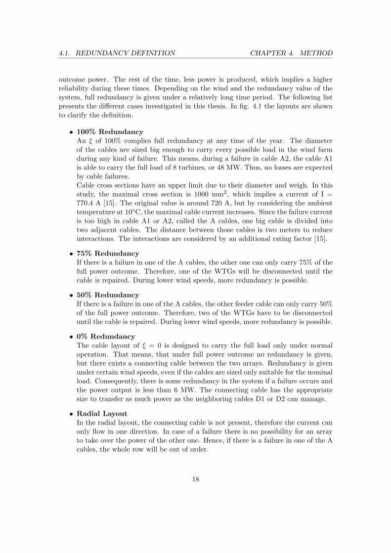
outcome power. The rest of the time, less power is produced, which implies a higherreliability during these times. Depending on the wind and the redundancy value of thesystem, full redundancy is given under a relatively long time period. The following listpresents the different cases investigated in this thesis. In fig. 4.1 the layouts are shownto clarify the definition.
• 100% RedundancyAn ξ of 100% complies full redundancy at any time of the year. The diameterof the cables are sized big enough to carry every possible load in the wind farmduring any kind of failure. This means, during a failure in cable A2, the cable A1is able to carry the full load of 8 turbines, or 48 MW. Thus, no losses are expectedby cable failures.Cable cross sections have an upper limit due to their diameter and weigh. In thisstudy, the maximal cross section is 1000 mm2, which implies a current of I =770.4 A [15]. The original value is around 720 A, but by considering the ambienttemperature at 10C, the maximal cable current increases. Since the failure currentis too high in cable A1 or A2, called the A cables, one big cable is divided intotwo adjacent cables. The distance between those cables is two meters to reduceinteractions. The interactions are considered by an additional rating factor [15].
• 75% RedundancyIf there is a failure in one of the A cables, the other one can only carry 75% of thefull power outcome. Therefore, one of the WTGs will be disconnected until thecable is repaired. During lower wind speeds, more redundancy is possible.
• 50% RedundancyIf there is a failure in one of the A cables, the other feeder cable can only carry 50%of the full power outcome. Therefore, two of the WTGs have to be disconnecteduntil the cable is repaired. During lower wind speeds, more redundancy is possible.
• 0% RedundancyThe cable layout of ξ = 0 is designed to carry the full load only under normaloperation. That means, that under full power outcome no redundancy is given,but there exists a connecting cable between the two arrays. Redundancy is givenunder certain wind speeds, even if the cables are sized only suitable for the nominalload. Consequently, there is some redundancy in the system if a failure occurs andthe power output is less than 6 MW. The connecting cable has the appropriatesize to transfer as much power as the neighboring cables D1 or D2 can manage.
• Radial LayoutIn the radial layout, the connecting cable is not present, therefore the current canonly flow in one direction. In case of a failure there is no possibility for an arrayto take over the power of the other one. Hence, if there is a failure in one of the Acables, the whole row will be out of order.
18
4.2. ENERGY CALCULATIONS CHAPTER 4. METHOD
• Average Wind Speed Layout (AWS)Since the layouts described above are designed for full power output, nearly allcables are oversized. That means, during most of the time, the flowing current ismuch less than the maximum possible current. This pushes up the investment costsunnecessarily and can be avoided by adapting the cable cross section to the averagecurrent flow. Taking the average windspeed into account, the corresponding powerflow is used to calculate the cable sizes. Each cable is therefore dimensioned toprovide 100% redundancy up to the average wind speed.
A1
B2
B1
A2 C2 D2
C1 D1
E
ξ = 75% ξ = 100% ξ = 50%
ξ = 0%
Figure 4.1: Different definitions of redundancies during a failure in cable A2 (correspondingto a failure in cable A1)
4.2 Energy Calculations
First, the kinetic energy has to be investigated by courtesy of the wind values A andk, which give information about the wind distribution. The Weibull curves are easilycalculated by eq. (3.2) and eq. (3.1), mentioned in the theory part. For comparisons,default values are set, which are shown in table 4.1.
19
4.3. GRID LOSSES CHAPTER 4. METHOD
Table 4.1: Default values
A (Weibull factor) 10.09
k (Weibull factor) 2.05
vm (mean wind speed) 9.8 m/s
cp 0.4
η 0.95
Cable installation costs 0.1 Me/km
Electricity price 0.25 e/kWh
Due to the unavailability of the power curve on the wind turbine data sheet, thepower curve is calculated. Hereby, the information In - and Off cut wind speeds areused of table 2.1, combined with the Betz limit, aerodynamic, mechanical and electricallosses. By taking all these informations into account the curve can be calculated usingeq. (3.4). The power curve is given in the results chapter.
Since the wind information is given, the focus is now put on the resulting power flowand the losses in the different layouts, introduced before. Depending on the selectedredundancy, the maximal power flow in each cable is calculated and compiled into avector. This is done by assuming a failure and defining the maximal possible power ineach cable. For example ξ = 100%, the maximum power in cable A1 or A2 would be8·6MW , whereas for ξ = 75% the A cables carry only the maximal power of for 7·6MW .Furthermore, the corresponding maximal current in each cable is calculated by eq.
I =P
V ·√
3. (4.1)
Knowing the flowing currents, the cable cross sections can be determined with the helpof a table from ABB [15]. The right cross section is necessary to provide a permanentpower flow without causing overload situations. The data sheet of ABB presents cablesfrom 95 mm2 till 1000 mm2, whereas the maximum current in the 1000 mm2 cable isaround 720 A. In case of exceeding the maximum, the current is divided up into twoequal cables, instead of using one big sized cable. Knowing the necessary diameters ofeach cable, the purchase costs can be investigated. Adding up the individual cable pricesand the installation costs of the system the capital price can be calculated. For furthercalculations, for each cable the resistances are determined, by using data from ABB [15].
4.3 Grid Losses
Knowing the resistance of the cables, cable losses can be calculated at any current. Forthis purpose, the data from the power and Weibull curves are used. For all wind speeds,the appropriate power outcome of the turbine and therefore the correlative currents are
20
4.4. FAILURE LOSSES CHAPTER 4. METHOD
known. Using the determined cable resistances, the losses can be calculated. By applyingeq. (3.7), a set of cable losses is provided, which demonstrate the losses as a function ofthe wind speed.In order to identify the total losses during a specific time period, the frequency of thewind speeds has to be taken into consideration. Hereby, the available Weibull wind datasare implemented like eq. (3.9). Losses are calculated with the assumption that the windpark is running in normal operation mode all year long. Failures are not subtracted fromthese losses, because it would be an insignificant amount of energy. Adding up the lossesduring the different wind speeds, the total losses are calculated by using eq. (3.10).
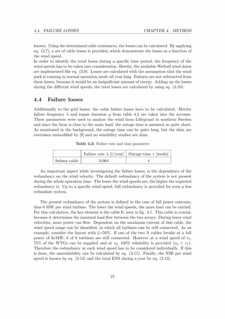
4.4 Failure losses
Additionally to the grid losses, the cable failure losses have to be calculated. Herebyfailure frequency λ and repair duration µ from table 4.2 are taken into the account.These parameters were used to analyze the wind farm Lillegrund in southern Swedenand since the farm is close to the main land, the outage time is assumed as quite short.As mentioned in the background, the outage time can be quite long, but the data areovertaken unmodified by [9] and no sensibility studies are done.
Table 4.2: Failure rate and time parameter
Failure rate λ [1/year] Outage time τ [weeks]
Subsea cable 0.004 4
An important aspect while investigating the failure losses, is the dependence of theredundancy on the wind velocity. The default redundancy of the system is not presentduring the whole operation time. The lower the wind speeds are, the higher the expectedredundancy is. Up to a specific wind speed, full redundancy is provided for even a lessredundant system.
The present redundancy of the system is defined in the case of full power outcome,thus 6 MW per wind turbine. The lower the wind speeds, the more load can be carried.For this calculation, the key element is the cable E, seen in fig. 4.1. This cable is crucial,because it determines the maximal load flow between the two arrays. During lower windvelocities, more power can flow. Dependent on the maximum current of this cable, thewind speed range can be identified, in which all turbines can be still connected. As anexample, consider the layout with ξ=50%. If one of the two A cables breaks at a fullpower of 6vMW, 6 of 8 turbines are still connected. However at a wind speed of v1,75% of the WTGs can be supplied and at v2, 100% reliability is provided (v2 < v1).Therefore the redundancy at each wind speed has to be considered individually. If thisis done, the unavailability can be calculated by eq. (3.11). Finally, the NSE per windspeed is known by eq. (3.12) and the total ENS during a year by eq. (3.13).
21
4.5. DIFFERENT LAYOUTS AND COMPARISON CHAPTER 4. METHOD
4.5 Different Layouts and Comparison
For comparison, the six different layouts are investigated. These layouts are explainedabove and are partly demonstrated in fig 4.1. Comparison is made by changing the pa-rameters, like wind speed, electricity price and installation costs. Changes in installationcosts is the easiest to implement, because the wind parameters and layout parametersremain the same. This is also true for the electricity price. The changes in wind speedare however more complicated. For each wind speed the Weibull factor A is changed,a new Weibull curve is needed and the losses change accordingly. Especially, the AWSlayout is more complicated, because the cross sections change with each loop. Thus,resistances and power losses vary extremely.
Since the main aim is to find out, if reduced redundancy results in lower costs thanfull redundancy, following central equation can be formulated:
whereas k>1 means, that full redundancy is the best solution and k<1 presents a morefavorable layout with less reliability. The results of the comparison are given in the nextchapter.
22
4.5. DIFFERENT LAYOUTS AND COMPARISON CHAPTER 4. METHOD
Create power curve and Weibull distribu4on
Calcula4ng the necessary cross sec4on to provide the desirable
redundancy at full power outcome
Determine the corresponding resistances in the individual cables
Calcula4ng the losses at the different wind speed levels
Failure losses in considera4on of the varying redundancy during
different wind speeds
Final investment analysis
Same opera4on for
• Radial • 0% • 50% • 75% • 100% • AWS layout
Lower wind speeds result in higher
reliability
Loop over power curve and
corresponding currents and
mul4plying with Weibull distribu4on
Figure 4.2: A visual demonstration of the calculation procedure to find the most appro-priate layout
23
5Results
In this thesis, the collection grid of a wind farm has been investigated in terms ofreliability, outlay costs and financial losses during 20 years of operation. Financial lossesdepend on the layout, the electricity price, the windspeed and the investment costs.
The total financial losses are studied, firstly for different electricity prices, secondlyfor variable wind speeds and thirdly, for different installation costs. It has to be men-tioned, that revenues are not added to the financial losses. Sensibility analyses, forvariable repair time of the cables, result in too insignificant changes compared to theother cases and are therefore not taken into account.
Fig. 5.1 shows the power curve of the wind turbine and also the two default weibullcurves. Since the ratio between reduced redundancy and full redundancy is investigated,the axes of the following figures are defined per unit and the 100% redundancy layout isset to 1.
5.1 Variable Electricity Price
The benefit of a wind turbine or a wind energy park depends highly on the revenues.Therefore, the electricity price is one of the most significant factors to investigate. Dueto laws, subsidies and changes in the economy, wind feed-in revenues change a lot, evenduring a small time scale. Fig. 5.2 gives an idea of how financial losses change by varyingenergy prices. To investigate the effect of the electricity price, the other parameters areset to the default values. The installation costs for the cables are 0.1 Me/km and theaverage windspeed is 9.7 m/s, whereas corresponding Weibull figures can be seen in fig.5.1.
Fig 5.2 demonstrates the development of the different layouts, as a function of theenergy price. At low energy prices, the installation costs have larger weight than thelosses during operation time and the system’s reliability is not as important. Therefore,the radial solution is the cheapest with a start value at around 1.4 Meuntil an energyprice of 5.1 ct
kWh . At this point, there is an intersection between the radial, ξ = 50% andthe average wind speed (AWS) layout. The latter, though, has a greater gradient and isthus not worth further mentioning. At 14.1 ct/kWh the 70% crosses the 50% layout andremains the most appropriate and beneficial solution.
Returning to the basic question, if less redundancy can result in less financial losses,fig. 5.2 gives an answer. It illustrates that 100% of reliability is definitely not the mostfavorable choice. The investments costs are much higher than probable losses during afailure. Compared to the layout with ξ = 75%, it is obviously not worth spending moneyto increase redundancy to 100%.
5.2 Variable Windspeed
The second investigation focuses on the average windspeed, which influences the powerproduction in a large scale. The higher the wind speeds during a year are, the higher therevenues become. Also, failures lead to greater losses of benefits. Fig. 5.3 illustrates thedevelopment of the losses, depending on the average windspeed. The electricity price is
set to the default value of 0.25 e/kWh and the cable installation costs to 0.1 Me/km.The layout with redundancy ξ = 50% is obviously the most suitable construction, sinceit is continuous the cheapest layout.
According to the European Energy Portal, in April 2010 the feed-in tariffs in Ger-many for wind offshore were around 0.13 - 0.15 e/kWh [27]. For a second analysis, theelectrical energy price is set to 0.14 e/kWh, apart from the remaining default values.In this case, quite overlapping results appear, which can be seen in fig. 5.4. The radialand the 0% layout surpass the costs for the full redundant system already below a windspeed of v = 8.5 m/s. Since the average wind speeds offshore are higher, these layoutsare not suitable. Below an average wind speed of 10 m
s the construction of ξ= 50% ismost suitable. At higher wind speeds ξ= 75% becomes lower.
The AWS layout results in a special curve, which totally deviates from the others.The reason for this difference is the definition of the layout design. Apart from the othercases, this design is dependent on the average wind speed. A more precisely layout de-scription can be found in chapter 4. The reason for this serrated curve is that for everywind speed the average power output changes. This change leads to a new calculationof the appropriate cross section every time. Thus, increasing windspeed, increases thecurrent in the cable, resulting in higher resistance losses, due to eq.(3.7). Because of thesquared current, the corresponding grid losses increase rapidly. At one point, the flowingcurrent exceed the limit of the maximum current in the actual cable size and a biggercable is taken, which leads to a step down after the peak. Thus, all the peaks ariseout of the changing cross section and the associated changing cable resistance losses.Generally the losses for this layout are incredibly high in the beginning, because at lowerwind speeds the cable sizes are at a minimum point and for all cables the smallest crosssection is chosen. Thus, compared to the other layouts, the resistances in the cables areimmensely high. In fig. 5.3 and 5.4 the curve has a minimum at a wind speed range of10.2-10.7 m/s and then suddenly rise and remain more or less equal. The abrupt increaseis the result of dividing up the current into two cables, which is discussed later.
Like the results before, the figure displays the financial differences between ξ = 100and ξ = [50, 75]. Similarly, 75% redundancy gives the most beneficial construction and100% exceeds the point where adding redundancy becomes more costly.
5.3 Variable Installation Costs
The case of variable installation costs is also implemented with the default values, anelectricity price of 0.25 e/kWh and the wind conditions shown in fig 5.1 and table 4.1.The result of changing installation costs are shown in fig. 5.5. Investigations of theinstallation costs of the cable are worth considering when the way of installation has tobe decided. As mentioned in chapter 2, the seabed conditions decides, which methodof cable laying can be applied. The cable installation is a fixed initial cost and results
therefore in the the same cost increase for all layouts. There are however two exceptions.Firstly, the radial layout costs are decreasing more sharply with rising installation costs,due to one cable less installed. Secondly, the full redundancy layout has two installedA cables instead of one, which causes a faster increase in investment costs. The onlyintersection occurs between the radial layout and the 100% layout at around 0.62 Me.However, the three most appropriate solutions are not involved in the intersection andremain the cheapest. Therefore, variable installation costs are not further investigated.
k (Cost ratio between reduced and full redundancy)
10
0 %
red
un
da
ncy
75
% re
du
nd
an
cy
50
% re
du
nd
an
cy
0%
red
un
da
ncy
rad
ial L
ayo
ut
AW
S
Figure 5.5: k as a function of the cable installation costs with the energy price of 0.25e/kWh and average wind speed of 9.7 m/s
31
5.4. CABLE LOSSES CHAPTER 5. RESULTS
5.4 Cable Losses
In the following table and figure, the cable cross sections and the respective losses at fullpower outcome (6 MW/turbine) are compared. These results are obtained regardless ofthe windspeed. Therefore, the average wind speed layout is not considered in this part,due to its wind speed dependance. Also, the radial layout is disregarded, because of itssimilarity to the 0% layout. In table 5.1 the individual cross sections of the cables aredemonstrated.
Table 5.1: Cable cross sections of the individual cables in each layout
Default windspeed v = 9.7 m/s
Redundancy ξCable Cross Section [mm2]
A1 B1 C1 D1 E D2 C2 B2 A2
0% 300 150 95 95 95 95 95 150 300
50% 630 500 300 150 95 150 300 500 630
75% 1000 630 500 300 150 300 500 630 1000
100% 2x300 1000 630 500 300 500 630 1000 2x300
According to eq. (3.7), the resistance constitutes the main part of the differencesbetween the losses, since the individual currents in the different cables are the same forall layouts at normal operation. For the normal operation in fig. 5.6, it is noticeablethat the 0% layout has extremely high grid losses, which is caused by the small crosssections, shown in table 5.1. In addition, it is conspicuous that from cable B1 to D1 orB2 to D2 the losses decline with increasing redundancy, due to the bigger cross sections.One exception is the feeder cable A1 or A2, in which the 100% layout surpass suddenlythe 75% and the 50%. The reason for this sharp increase of losses is the double cable.As mentioned before, the cable A1 and A2 in ξ = 100% consists of two cables. The totalcurrent is too high and can not be carried by the biggest cable with a cross section 1000mm2. Therefore the current is halved and cables with suitable sizes are chosen, whichresult in two times 300 mm2. It is noticeable, that the total cross section of the twocables is smaller than 1000 mm2. The reasons for that are explained more precisely inthe discussion.
32
5.4. CABLE LOSSES CHAPTER 5. RESULTS
A B C D E D C B A0
50
100
150
200
250
300
350
400
450
Cables
Curr
ent
Normal Operation
A B C D E D C B A0
1
2
3
4
5
6
7x 10
4
Cables
Losses
Resistance Losses
0 % redundancy
50% redundancy
75% redundancy
100% redundancy
Figure 5.6: Currents and losses in normal operation
33
6Discussion
6.1 Discussion
The fig. 5.2, 5.3, 5.4 and 5.5 show six different layouts dependent on three differentparameters. For a better comparison, the parameters are fixed to the default values,a wind speed of v = 9.7 m/s, an energy price of 0.25 e/kWh and installation costs of100000 e/km. In the fig 6.1 the layouts with ξ = 0, 50, 75 and 100 are illustrated toclarify the results. A minimum can be seen around 70-75%. Important to notice is thatthe curve is only valid for the interval of 0 to 100.
The average wind speed layout is not taken into account, because the curve variesextremely by changing the wind speed. Besides, the reliability definition, compared tothe other layouts, is too deviating to make an adequate comparison. A more precisediscussion about this curve is made later in this section. Also, the radial layout is leftout of consideration, because it is related to the 0% layout. As in fig. 6.1 can be seen,the interpolated curve presents a minimum cost at a redundancy around 70%. But sinceit is a spline and only four different cases are investigated, the real curve progressioncan not been defined. A fact to be emphasized, is the definition of redundancy. Asmentioned previously, the redundancy has no uniform definition, but the results are ex-tremely dependent on that. The clear meaning of redundancy in this thesis is discussedin the method chapter.
An interesting aspect is also the intersection between the ξ = 75% and ξ = 100% in fig5.2, which denotes the electricity price, where the full redundancy design becomes morebeneficial. However, in these results, the costs of ξ=100% increase faster and thereforefull redundancy will never be the cheapest layout. Since it has no failure losses it shouldconsequentially become cheaper at a certain energy price. But it has to be consideredthat the costs, caused by resistance losses carry more weight than outages. It can be
34
6.1. DISCUSSION CHAPTER 6. DISCUSSION
Figure 6.1: Graph of costs of the 0%, 50%, 75% and 100% layouts in the intverval of [0100]
−25 0 25 50 75 100 1252000
2500
3000
3500
4000
4500
5000
5500
6000
Costs
[k
Euro
]
Redundancy [%]
noted generally, that the higher the redundancy, the larger the cable sizes and thereforethe lower the grid losses. However, this is not applicable for the full redundancy layout,since the A cables are divided. The resistances by ABB have no linear behavior and thesame thermal resistance ( = 1Km/W) is assumed for all cables [15]. Smaller cables havea better heat dissipation and can therefore manage higher currents per mm2. For thisreason, half the current requires less than half the cross section. The cross sections aresmaller and have therefore higher resistances and also higher losses. In this regard, di-viding the current and calculating a suitable new cross section is pointless. This problemcan be solved in better ways. The installation of two cables with the area of 1000 mm2
would lower the grid losses but also rise the investment and installation costs immensely.Also a cable with a cross section greater than 1000 mm2 could be produced to increasethe possible maximum current in the cable.
It is important to point out that the thermal dependency influences the cable resis-tances extremely. In this thesis, the resistances for calculating the grid losses are usedfrom the ABB cable data sheet and are kept constant during the entire calculations[15]. The seabed is assumed to be 10C, which is beneficial regarding the maximum
35
6.2. CONCLUSION CHAPTER 6. DISCUSSION
temperature in the cables. To adapt the parameter, a rating factor is added, whichincreases the current limit in a cable by 7% [15]. Apart from external impacts the cableheating in itself is also crucial. The electrical resistance is temperature dependent andincreases when the current is rising. At high wind speeds, the current is higher and thecable becomes warmer. The changes in resistance can become rather significant, sincethe temperature difference ∆T in the conductor can rise up to 70 K. That would implyapproximately a 27% higher resistance, but most of the times the currents are belowthe maximal cable current, what keeps the effect within limits. If instead of a constantresistance, a resistance as a function of the temperature is used, the losses at high windspeeds increase even more sharply. When comparing the different layouts, the slope ofthe curve changes in all cases, but with a different intensity. On the one hand, the currentin the smaller cables reaches the limit faster, whereas on the other hand, the heat dissipa-tion of the big cables is worse. For an exact investigation, this facts should be considered.
When taking a closer look at the average layout, it is difficult to draw a clear con-clusion. Calculating a new cross section for each wind speed leads to an array of curves.The composition of those by hopping from one curve to another, results in this jaggedappearance. Compared to the other graphs, it leaves doubts about its practical usability.However, it is reasonable to observe thoroughly the wind speeds for designing the cablesizes. In figures 5.3 and 5.4, the minimum occurs at around v = 10.5 m/s, which is inthe range of average offshore wind speeds. Moreover, the curve shows the dependanceof grid losses on cable sizes. Designing cables with suitable sizes for the expected powerflow, creates unnecessary high ohmic losses in the most cases. This outcome fits theadvice of ABB to avoid losses by using larger cable diameters [15] . Thus, saving incable outlay costs returns a lower benefit of the produced wind power. This statementis however only valid up to a certain point, the minimum at v = 10.5 m/s. Above theminimum, a sharp increase occur due to the split into two lines. Dividing the current intwo smaller cables, rises the resistance enormously and is also a sign for an inconvenientdesign. At the minimum, the AWS design overlaps with the 75% layout, the presumablymost beneficial solution. Apparently, the cable sizes reach an optimum at this point,confirming the quality of the 75% redundancy solution. Consequently, the outcome ofthe fig. 6.1 is confirmed by the average layout design.
6.2 Conclusion
By implementing the three different cases, a remarkable difference in the financial lossesturned out. Referring to the aim of the thesis and the corresponding eq. (4.2) in chapter4, the statement that lowering redundancy results in less costs, is verified. In all studiedcases the investigation results in k<1.
36
6.3. FUTURE WORK CHAPTER 6. DISCUSSION
Inserting the default values from table 4.1, k results in
k =Cξ=75%
Cξ=100%= 0.87. (6.1)
In summary, reducing the redundancy in a collection grid results in a greater benefit.For this thesis, a redundancy around 70-75% of reliability is the best solution.
6.3 Future Work
In this study only a few cases are picked out to mark the differences. For a full inves-tigation, a reliable optimum for each individual wind speed and electricity price has tobe found. For this purpose, a optimization in several dimensions could help to depicte.g. cross sections over price and wind speed at the same time. To find a general fi-nancial optimum, additional components have also to be considered, such as breakers,switchers and other power electronics. Also a sensitivity study is missing in this thesisto demonstrate possible changes if two cable break simultaneously or if a damage is toocomplicated and demand more repair time than expected. Currently, the energy sectorfocuses a lot on the development of the electrical grids. Several conferences and stud-ies discuss the sophisticated integration of renewable energies and the appropriate gridcapacities [28].
37
Bibliography
[1] P.-E. Morthorst, Wind energy the facts volume 2 - costs and prices, Tech. rep.,EWEA, European Wind Energy Association (2004).
[2] Z. Chen, F. Blaabjerg, Wind farm - a power source in future power systems, Re-newable and Sustainable Energy Reviews 13 (6-7) (2009) 1288–1300.
[3] A. Sannino, H. Breder, E. Nielsen, Reliability of collection grids for large offshorewind parks, in: Probabilistic Methods Applied to Power Systems, 2006. PMAPS2006. International Conference on, 2006, pp. 1 –6.
[4] M. Rock, . Parsons, Laura, Offhore Wind Energy, [online] Available at:<www.eesi.org/files/offshore wind 101310.pdf>[Accessed 06 December 2012].
[6] Offshore Wind, 2012, [online] Available at <http://www.ewea.org/policy-issues/offshore/>, [Accessed 04 December 2012].
[7] B. Franken, H. Breder, M. Dahlgren, E. Nielsen, Collection grid topologies for off-shore wind parks, in: Electricity Distribution, 2005. CIRED 2005. 18th InternationalConverence and Exhibition on, 2005.
[8] P.-E. Morthorst, S. Awerbuch, The economics of wind energy, Tech. rep., The Eu-ropean Wind Energy Association (March 2009).
[9] E. Eriksson, Wind farm layout - a reliability and investment analysis, Master’sthesis, Uppsala Universitet, Teknisk- naturvetenskaplig fakultet UTH-enheten (Oc-tober 2008).
[10] J. Yang, J. O’Reilly, J. E. Fetcher, Redundancy analysis of offshore wind farmcollection and transmission systems, in: Sustainable Power Generation and Supply,2009, SUPERGEN ’09. International Conference on, 2009, pp. 1–7.
38
BIBLIOGRAPHY BIBLIOGRAPHY
[11] Siemens, 2011, Juni, Prototyp der neuen getriebelosen 6-MW-Windturbine von Siemens geht in Testbetrieb [Online] Available at:,<http://www.siemens.com/press/de/pressemitteilungen/?press=/de/pressemitteilungen/2011/renewable energy/ere201106070.htm>,[Accessed 02 December 2012].
[12] Siemens, Wind turbine with the world’s largest rotor goes into operation, 2012,[online] Available at: <www.siemens.com/press/en/feature/2012/energy/2012-07-rotorblade.php>, [Accessed 04 December 2012].
[14] The World of Wind Atlases-Wind Atlases of the World, 2011, RisøNational Labo-ratory for Sustainable Energy, Technical University of Denmark, [online] Availableat: <www.windatlas.dk>, [Accessed 04 December 2012].
[15] ABB, 2010, XLPE Land Cable System User’s Guide, [online] Available at<www.05.abb.com>, [ Accessed 05. December 2012].
[16] U. Gudmundsdottir, C. Bak, W. Wiechowski, Modeling of long high voltage ac un-derground cables, PhD with the Institute of Energy Technology, Aalborg University.
[17] Jimmy Ehnberg 2012, Chalmers University of technology, pers. comm., 14 Septem-ber.
[18] ABB, 2012, XLPE Submarine Cable Systems - Attachment toXLPE Land Cable Systems - User’s guide, [online] Available at:<www.abb.com/abblibrary/downloadcenter/?View=Result> [Accessed 04 De-cember 2012].
[19] J. Ehnberg, Lektion kabelforlaggning offshore - Elsystem for vindkraft, HogskolanVast.
[20] A. Larsson, O. Unosson, Offshore cable installation, Tech. Rep. 30, Vattenfall (Jan-uary 2009).
[21] E. Hau, Wind turbines - Fundamentals, Technologies, Applications, Economics,Berlin : Springer, cop.2000, 2000.
[22] The free dictionary, 2012, [online] Available at: <www.thefreedictionary.com>, [Ac-cessed 03 December 2012].
[23] J. Seguro, T. Lambert, Modern estimation of the parameters of the weibull dis-tribution for wind energy analysis, Journal of Wind Engineering and IndustrialAerodynamics 85 (1) (2000) 75–84.
39
BIBLIOGRAPHY
[24] R. Gasch, J. Twele, Windkraftanlagen: Grundlagen, Entwurf, Planung und Betrieb,6th Edition, Vieweg + Teubner, 2010.
[25] H.-J. Wagner, J. Mathur, Physics of wind energy, in: Introduction to Wind EnergySystems, Green Energy and Technology, Springer Berlin Heidelberg, 2009, pp. 17–28.
[26] N. Negra, O. Holmstrøm, B. Bak-Jensen, P. Sorensen, Aspects of relevance in off-shore wind farm reliability assessment, Energy Conversion, IEEE Transactions on22 (1) (2007) 159–166.
[27] Europeans Energy Portal, 2012, [online] Available at <www.energy.eu> [Accessed04 December 2012].
[28] Wind Energy The Facts Part II - Grid Integration, [online] Available at<www.wind-energy-the-facts.org/documents/download/Chapter2.pdf> [Accessed 07 December2012].