UNIVERSITY OF CALIFORNIA Los Angeles Improving LDPC Decoders: Informed Dynamic Message-Passing Scheduling and Multiple-Rate Code Design A dissertation submitted in partial satisfaction of the requirements for the degree Doctor of Philosophy in Electrical Engineering by Andres Ivan Vila Casado 2007
Transcript
UNIVERSITY OF CALIFORNIA
Los Angeles
Improving LDPC Decoders: Informed Dynamic
Message-Passing Scheduling and Multiple-Rate
Code Design
A dissertation submitted in partial satisfaction of the
1.1 Digital Communication System . . . . . . . . . . . . . . . . . . . . 11.2 Factor graph of a rate-1/2 LDPC code . . . . . . . . . . . . . . . . 7
2.1 FER vs. number of iterations of a blocklength-1944 rate-1/2 codeusing flooding, LBP, RBP, ARBP, NS and ANS for a fixed Eb/No =1.75 dB. . . . . . . . . . . . . . . . . . . . . . . . . . . . . . . . . . 23
2.2 FER vs. number of iterations of the 802.11n blocklength-1944 rate-1/2 code using flooding, LBP, ARBP and ANS for a fixed Eb/No =1.75 dB. The dashed line indicates the expected performance of ARBP. 24
2.3 FER vs. number of iterations of the 802.11n blocklength-1944 rate-5/6 802.11n code using flooding, LBP, ARBP and ANS for a fixedSNR = 6.0 dB. The dashed line indicates the expected performanceof ARBP. . . . . . . . . . . . . . . . . . . . . . . . . . . . . . . . . 25
2.4 Check-node update sequence that solves a trapping set. On the leftside, the figure shows the sub-graph induced by a set of variablenodes in error and their nearest-neighbor check nodes. On the rightside the figure shows the new sub-graph that results after ANS cor-rects a variable node, thus removing it from the sub-graph. Shadednodes represent the check node that is updated and the variablenode that is corrected. . . . . . . . . . . . . . . . . . . . . . . . . . 27
2.5 AWGN performance of the blocklength-2640 Margulis code decodedby 3 different scheduling strategies: flooding, LBP and ANS. Amaximum of 50 iterations was used. . . . . . . . . . . . . . . . . . . 28
2.6 AWGN Performance of code A vs. number of iterations for a fixedEb/No = 3 dB. Results of 5 different scheduling strategies are pre-sented: flooding, LBP, ANS, F-LBP/ANS with ξ = 35 and A-LBP/ANS with ζ = 5. . . . . . . . . . . . . . . . . . . . . . . . . . 33
2.7 AWGN performance of code C decoded by 5 different schedulingstrategies: flooding, LBP, ANS, F-LBP/ANS with ξ = 35 and A-LBP/ANS with ζ = 5. . . . . . . . . . . . . . . . . . . . . . . . . . 34
vi
2.8 AWGN performance of a blocklength-1944 LDPC code decoded by6 different scheduling strategies: flooding, LBP, ANS, A-LBP/ANSwith ζ = 5, LC-ANS and P-ANS. . . . . . . . . . . . . . . . . . . . 37
2.9 AWGN Performance of a blocklength-1944 LDPC code vs. num-ber of iterations for a fixed Eb/No = 2 dB. Results of 5 differentscheduling strategies: flooding, LBP, ANS, A-LBP/ANS with ζ = 5,LC-ANS and P-ANS. . . . . . . . . . . . . . . . . . . . . . . . . . . 38
3.1 Graph of a rate-3/4 LDPC code obtained from a rate-1/2 LDPCcode via row combining. . . . . . . . . . . . . . . . . . . . . . . . . 42
with blocklength 1944 on an AWGN channel. Maximum number ofiterations equal to 15. . . . . . . . . . . . . . . . . . . . . . . . . . . 55
3.4 Performance of structured SRC with p=54, structured RCEV, andIEEE 802.11n codes with blocklength 1944 on an AWGN channel.Maximum number of iterations equal to 50. . . . . . . . . . . . . . 57
3.5 Performance of RCEV codes and punctured LDPC codes. . . . . . . 593.6 Sphere-packing bound gap at a FER of 10−3 between row-combining
codes and punctured codes. Both codes have the same rate (9/10)and have equal mother-code blocklength. The mother code of thepunctured codes has rate 1/2. . . . . . . . . . . . . . . . . . . . . . 60
vii
List of Tables
2.1 FER and UFER of 5 different LDPC codes decoded by 5 differentscheduling strategies: flooding, LBP, ANS, F-LBP/ANS with ξ = 35and A-LBP/ANS with ζ = 5. The channel used is AWGN withEb/No = 3 dB. . . . . . . . . . . . . . . . . . . . . . . . . . . . . . 31
In fact, the exploitation of such parallelism requires the use of several check-and
variable-node processors, each connected to different memories in order to access
several messages simultaneously. The random character of the node connection in
the factor graph results in difficult memory/processor placement and intractable-
routing problems.
In order to solve these problems, LDPC codes can be designed to have an in-
herent structure as suggested by Mansour and Shanbag in [30]. This approach also
enables the implementation of high -speed decoders without memory fragmenta-
tion such as those presented in [31] and [32]. In [30] the LDPC matrices have a
block structure that consists of square sub-matrices each of size p. Each square
sub-matrix is either a zero sub-matrix or a structured sub-matrix.
An example that illustrates the structured sub-matrices proposed in [30] for
p = 4, is shown in (1.10). This sub-matrix, labelled as S2, results from performing
a right cyclic shift of 2 columns on the identity matrix of size p. Each sub-matrix
Si is produced by cyclically shifting the columns of an identity matrix to the right
i places,
S2 =
0 0 1 0
0 0 0 1
1 0 0 0
0 1 0 0
. (1.10)
This structured LDPC matrix allows the decoder to use at least p processors
in parallel and doesn’t preclude the implementation of faster decoders that use a
multiple of p processors as suggested in [33].
10
1.2.4 Analog Decoders
Analog decoders of turbo-like codes were introduced simultaneously in 1998 by Ha-
genauer [34] and Loeliger et al. [35]. A good in-depth discussion of this alternative
decoding hardware can be found in [36]. They propose to use several small analog
circuits that perform the message-generation operations and to interconnect them
according to the code graph.
Thus, analog decoders are analog circuits that oscillate until an equilibrium
state is reached. Analog decoding shows promise because the decoders require low
power and the convergence is typically faster than with digital decoders. Digi-
tal decoders can use the same hardware to decode different LDPC codes by re-
programming the signal processing circuit. Their analog counterparts are not pro-
grammable, and they require different circuits to decode different LDPC codes.
Since many applications need various codes to support different data rates, the
lack of programmability of analog decoders makes them less attractive than dig-
ital decoders when it comes to LDPC codes. However, the row-combining codes
presented in this dissertation allow programmable analog decoders as will be seen
in Chapter 3.
1.2.5 Low-Complexity Encoding Using Back Substitution
The parity-check matrix should also allow a simple encoder implementation. Sys-
tematic codes are desirable for simple encoders. A code is deemed systematic if
the k information bits are part of the codeword. Thus, systematic-code codewords
can be divided into k information (or systematic) bits and (n − k) parity bits.
Encoding consist of computing the (n− k) parity bits based on the k information
bits. In [37] and [38] a low-complexity encoder for systematic LDPC codes is found
if its parity-check matrix H0 is composed of two matrices H0 = [H1|H2] where H2
is a square sub-matrix that has a particular structure. H1 is a (n− k)× k matrix
whose columns correspond to the k information bits. H2 is a (n − k) × (n − k)
matrix whose columns correspond to the (n − k) parity bits. With this special
structure, encoding complexity grows linearly with the code length.
11
A code that where H2 is a lower triangular matrix allows a low-complexity
encoder based on back-substitution as explained in [38]. Back substitution obtains
the parity bits by solving sequentially the parity-check equations. The first (top)
row of H0 has only one unknown, the first parity bit. Since H2 is lower triangular,
once the value of that first parity bit is known, the second equation is guaranteed
to have at most one unknown, the second parity bit. In that fashion, each parity-
check equation is solved sequentially until all the parity bits are generated, which
happens when the bottom row is solved. As an example let us take the following
LDPC code
H0 =
1 1 1 0
1 0 0 1
0 1 0 0︸ ︷︷ ︸
H1
∣∣∣∣∣∣∣∣
1 0 0
1 1 0
1 1 1
︸ ︷︷ ︸H2
. (1.11)
Eq. (1.11) shows a parity-check matrix where H2 is lower triangular. Back-
substitution encoding starts by solving the top parity-check equation for the first
parity bit. Thus, we compute the first parity bit as the sum modulo-2 of the
first three information bits. With that information we proceed to solve the middle
parity-check equation. This middle row indicates that the second parity bit is equal
to the sum modulo-2 of the first and fourth systematic bits and the first parity bit.
Finally the last parity bit is computed by adding the second information bit with
the first and second parity bits as indicated by the bottom parity-check equation.
1.2.6 LDPC Code Design
Designing good LDPC codes appears at first to be a daunting task. Fortunately,
the design process can be divided in two distinct tasks that allow a straightforward
design procedure. The first task is to design good variable-node and check-node
degree distributions. A degree distribution describes the percentage of nodes of
each degree. For example, variable-node degree distribution can state that 15% of
the variable-nodes must have degree 13, 35% of the nodes degree 3, and 50% of the
12
nodes degree 2. In [39], Richardson and Urbanke developed the density evolution
algorithm which computes the average Bit-Error Probability (BER) of an LDPC
code based only on its check-node and variable-node degree distributions. Density
evolution results are valid for asymptotically large blocklengths and ML decoders.
They showed that LDPC codes with different variable-node and check-node degree
distributions have different error-correcting behavior. This allows the design of the
degree distributions independently from the actual blocklength and realization of
the code.
Once the degree distributions are chosen, the second task is to construct the H
according to the selected degree distributions. There are several code construction
algorithms that share the same objective: to minimize the negative effects of BP
decoding. BP is not ML because there are loops in the factor-graph representation
of the code. Once possible approach is to construct the code while maximizing the
girth of the factor graph [40]. A different design approach is to identify and avoid
the most harmful loops [41], [42]. This second approach will be presented in detail
in Section 3.4.
1.3 Outline
The rest of the dissertation is organized as follows: Chapter 2 introduces the con-
cept of IDS as well as several strategies that work well for different scenarios such
as low-complexity decoders, short-blocklength LDPC codes and high-throughput
applications. Chapter 3 describes the row-combining approach in detail as well as
different multiple-rate LDPC code design algorithms based on the row-combining
idea. Chapter 4 delivers the overall conclusions.
The main contributions of the work presented in this dissertation are:
• The introduction of Informed Dynamic Scheduling for LDPC BP decoding
(Chapter 2).
• An understanding of the behavior and advantages of IDS LDPC decod-
ing when compared with traditional message-passing scheduling strategies
13
(Chapter 2).
• IDS strategies for short-blocklength LDPC codes (Chapter 2).
• Low complexity and high throughput IDS strategies (Chapter 2).
• The introduction of row-combining as a tool to design multiple-rate LDPC
code with constant blocklength. This contribution is significant for both
digital and analog decoder implementations (Chapter 3).
• Two algorithms to design row-combining multiple-rate LDPC codes for dif-
ferent applications (Chapter 3).
14
Chapter 2
LDPC Decoders with Informed
Dynamic Scheduling
As mentioned in Chapter 1, Belief Propagation (BP) provides Maximum-Likelihood
(ML) decoding over a cycle-free factor-graph representation of a code as shown
in [21] and [15]. In some cases, BP over loopy factor graphs of channel codes has
been shown to have near-ML performance. BP performs well on the (loopy) bi-
partite factor graphs composed of variable nodes and check nodes that describe
LDPC codes.
However, loopy BP is an iterative algorithm and therefore requires a message-
passing schedule. Flooding, or simultaneous scheduling, was the first scheduling
strategy. In flooding scheduling, an iteration consists of the simultaneous update
of all the messages mv→c followed by the simultaneous update of all the messages
mc→v.
Recently, several papers have addressed the effects of different types of sequen-
tial, or non-simultaneous, scheduling strategies in BP LDPC decoding. With se-
quential scheduling, the messages are generated sequentially using the latest avail-
able information. The idea was introduced as a sequence of check-node updates
in [24] and as a sequence of variable-node updates in [25]. It is also presented in [26]
under the name of Layered BP (LBP), in [27] as a serial schedule, in [28] as shuf-
fled BP, in [29] as row message passing, column message passing and row-column
15
message passing, among others.
Monte-Carlo simulations and theoretical analysis in [43]- [29] show that se-
quential scheduling converges twice as fast as flooding when used in LDPC decod-
ing. It has also been shown that sequential updating doesn’t increase the decod-
ing complexity per iteration, thus allowing the convergence speed increase at no
cost [29], [44]. Furthermore, the various types of static sequential schedules dis-
cussed above have very similar performance results [29]. In this dissertation, the
sequential-scheduling strategy used for comparison is LBP, a sequence of check-
node updates, as presented in [24] and [26]. As an example, a possible LBP sched-
ule is described in Algorithm 1. The algorithm stops if the decoded bits satisfy all
the parity-check equations or a maximum number of iterations is reached.
Algorithm 1 LBP decoding for LDPC codes
1: Initialize all mc→v = 02: Initialize all mvj→ci
= Cj
3: for every i ∈ {1, . . . , M} do4: for every vk ∈ N (ci) do5: Generate and propagate mci→vk
6: for every ca ∈ N (vk) \ci do7: Generate and propagate mvk→ca
8: end for9: end for
10: end for11: if Stopping rule is not satisfied then12: Position=3;13: end if
Sequential updating introduces the problem of finding the ordering of message
updates that results in the best convergence speed and/or code performance. The
current state of the messages in the graph can be used to dynamically update
the schedule, producing what we call Informed Dynamic Scheduling (IDS). We
presented IDS in [45] and first published it in [46]. To our knowledge, the only
well-defined IDS strategy, other than the work presented in this dissertation, is the
Residual Belief Propagation (RBP) algorithm [47]. RBP was proposed for general
sequential message passing, not specifically for BP decoding.
16
RBP is a greedy algorithm that organizes the message updates according to
the absolute value of the difference between the message generated in the current
iteration and the message generated in the previous iteration. The intuition is that
the larger this difference, the further from convergence this part of the graph is.
Therefore, propagating this message first will make BP converge at a higher speed.
Simulations show that RBP LDPC decoding has a higher convergence speed
than LBP but its error-rate performance for a large enough number of iterations
is worse. This behavior is commonly found in greedy algorithms, which tend to
arrive at a solution faster, but arrive at the correct solution less often. We propose
a less-greedy IDS strategy in which all the outgoing messages of a check-node are
generated simultaneously. We call it Node-wise Scheduling (NS) and it converges
both faster and more often than LBP.
Both RBP and NS require the knowledge of the message to be updated in order
to pick which message to update. This means that many messages are computed
and not passed. This increases the complexity of the decoding per iteration. We
use the min-sum check-node update [22] [23] described in (1.9), to simplify the
ordering metric and significantly decrease the complexity of both strategies while
maintaining the same performance.
We study the behavior of IDS for different types of codes and applications such
as short-blocklength LDPC codes, parallel decoders and lower-complexity decoders.
We propose appropriate IDS strategies that work well for these applications.
This chapter is organized as follows. Section 2.1 introduces RBP and NS for
LDPC decoding as well as the min-sum IDS strategies. It also gives intuitive
explanations for their performance and analyzes their behavior in the presence
of traditional trapping-set errors. Section 2.2 analyzes the behavior of IDS on
short-blocklength LDPC codes and introduces strategies that perform better in
this scenario. Section 2.3 introduces schedules more suitable for hardware imple-
mentation such as a lower-complexity IDS strategy and a parallel IDS strategy.
Section 2.4 delivers the conclusions of this chapter. Simulation results of the vari-
ous message-passing schedules are presented along the way.
17
2.1 Informed Dynamic Scheduling (IDS)
2.1.1 Residual Belief Propagation (RBP)
RBP, as introduced in [47], is an IDS strategy that updates messages according
to an ordering metric called the residual. The message with the largest residual
is updated first. A residual is the norm (defined over the message space) of the
difference between the values of a message before and after an update. For a
message mni→njthat goes from node ni to node nj, the residual is defined as:
r(mni→nj
)=
∥∥∥mnewni→nj
−moldni→nj
∥∥∥ , (2.1)
where the superscript new denotes the message to be propagated now and old
denotes the message that was propagated the last time mni→njwas updated.
The intuition behind this approach is that as loopy BP converges, the residuals
go to zero. Therefore, if a message has a large residual, it means that it’s located in
a part of the graph that hasn’t converged yet. Therefore, propagating that message
first should speed up the process.
In LLR BP decoding, all the message spaces are one-dimensional (the real line).
Hence, the residuals are the absolute values of the differences of the LLRs.
Let us analyze the behavior of RBP decoding for LDPC codes in order to
simplify the decoding algorithm. Initially, all the messages mv→c are set to the
value of their corresponding channel message Cv. No operations are needed in this
initialization. This implies that the residuals of all the variable-to-check messages
r(mv→c) are equal to 0. Then, without loss of generality, we assume that the
message mci→vjhas residual r∗, which is the largest of the graph. After mci→vj
is
propagated, only residuals r(mvj→ca) change, with ca ∈ N (vj) \ci.
The new residuals r(mvj→ca) are equal to r∗ because r∗ was the change in the
message mci→vjand (1.7) shows that the message-update operations of a variable
node are sums. Therefore, the messages mvj→ca have now the largest residuals in
the graph.
Assuming that propagating the messages mvj→ca won’t generate any new resid-
18
uals bigger than r∗, RBP can be simplified. Every time a message mc→v is propa-
gated, the outgoing messages from the variable node v will be updated and prop-
agated. After propagation of the messages from the variable node v, all residuals
for messages from variable nodes are again zero. This facilitates the scheduling
since we need only to search for the largest r(mc→v) in order to find out the next
message to be propagated. RBP LDPC decoding is formally described in Algo-
rithm 2. Another way to implement RBP, presented in [47], is to create a priority
queue of messages, ordered by the value of their residuals, so at each step the first
message in the queue is updated and then the queue is reordered using the new
information.
Algorithm 2 RBP decoding for LDPC codes
1: Initialize all mc→v = 02: Initialize all mvj→ci
= Cj
3: Compute all r(mc→v)4: Find r(mci→vj
) = max r(mc→v)5: Generate and propagate mci→vj
6: Set r(mci→vj) = 0
7: for every ca ∈ N (vj) \ci do8: Generate and propagate mvj→ca
9: for every vb ∈ N (ca) \vj do10: Compute r(mca→vb
)11: end for12: end for13: if Stopping rule is not satisfied then14: Position=4;15: end if
There is an intuitive way to see how RBP decoding works for LDPC codes. Let
us assume that at a certain moment in the decoding, there is a check node ci with
residuals r(mci→vb) = 0 for every vb ∈ N (ci). Now let us assume that there is a
change in the value of the message mvj→ci. It can be proven that the largest change
in a check-to-variable message out of ci (therefore the largest residual) will occur
in the edge that corresponds to the incoming variable-to-check message with the
lowest reliability (excluding the message mvj→ci). Let us denote by vk the variable
node that is the destination of the message that has the largest residual r(mci→vk).
19
Then, the message mvk→cihas the smallest reliability out of all messages mvb→ci
,
with vb ∈ N (ci) \vj.
This implies that, for this particular scenario, once there’s a change in a
variable-to-check message, RBP will propagate first the message to the variable
node with the lowest reliability. This makes sense intuitively because the lowest-
reliability variable node is more likely to be in error than the higher-reliability
nodes.
The negative effects of the greediness of RBP are apparent in the case of unsat-
isfied check nodes connected to only one variable node in error. RBP will schedule
to propagate first the message that will “correct” the variable node with the lowest
reliability. Again, this is the most likely variable node to be in error. However,
if that variable node was already correct, the variable node in error will not be
corrected and there will be one more error. The information from this new error
will likely be propagated next because the largest changes in incoming messages
tend to induce the largest residuals. This analysis helps us see why RBP corrects
the most likely errors faster but has trouble correcting “difficult” errors as will be
seen in the performance plots. We define “difficult” errors as the errors that need
a large number of message updates to be corrected.
2.1.2 Node-wise Scheduling Decoding for LDPC Codes
In order to obtain a better performance for all types of errors, perhaps a less greedy
scheduling strategy must be used. As noted earlier, some of the greediness of RBP
came from the fact that it tends to propagate first the message to the least reliable
variable node. We propose to update and propagate simultaneously all the check-
to-variable messages that correspond to the same check node ci, instead of only
propagating the message with the largest residual r(mci→vj). It can be seen, using
the analysis presented earlier, that this algorithm is less likely to propagate the
information from new errors in the next update. This is due to the fact that there
are many variable nodes that change as opposed to RBP where only one variable
node changes. We call this less greedy strategy Node-wise Scheduling (NS).
20
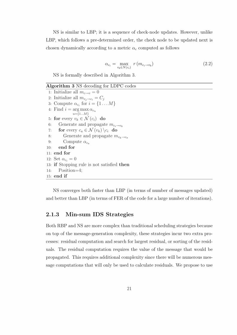
NS is similar to LBP; it is a sequence of check-node updates. However, unlike
LBP, which follows a pre-determined order, the check node to be updated next is
chosen dynamically according to a metric αc computed as follows
αci= max
vb∈N(ci)r (mci→vb
) (2.2)
NS is formally described in Algorithm 3.
Algorithm 3 NS decoding for LDPC codes
1: Initialize all mc→v = 02: Initialize all mvj→ci
= Cj
3: Compute αcifor i = {1 . . .M}
4: Find i = arg maxu={1...M}
αcu
5: for every vk ∈ N (ci) do6: Generate and propagate mci→vk
7: for every ca ∈ N (vk) \ci do8: Generate and propagate mvk→ca
9: Compute αca
10: end for11: end for12: Set αci
= 013: if Stopping rule is not satisfied then14: Position=4;15: end if
NS converges both faster than LBP (in terms of number of messages updated)
and better than LBP (in terms of FER of the code for a large number of iterations).
2.1.3 Min-sum IDS Strategies
Both RBP and NS are more complex than traditional scheduling strategies because
on top of the message-generation complexity, these strategies incur two extra pro-
cesses: residual computation and search for largest residual, or sorting of the resid-
uals. The residual computation requires the value of the message that would be
propagated. This requires additional complexity since there will be numerous mes-
sage computations that will only be used to calculate residuals. We propose to use
21
the min-sum check-node described in (1.9) to compute the approximate-residuals
as follows,
rni→nj(mk) =
∥∥∥mnewni→nj
− moldni→nj
∥∥∥ , (2.3)
where the tilde indicates the min-sum approximation. Using approximate-residual
functions in Algorithms 2 and 3, defines Approximate RBP (ARBP) decoding and
Approximate NS (ANS) decoding. These significantly simpler algorithms perform
as well as the ones presented in Section 2.1. Note that we only propose to use
min-sum for the residual computation. For the actual propagation of messages we
use the full update equations (1.7) and (1.8).
We compare the performance of traditional scheduling strategies and IDS strate-
gies after the same number of messages are propagated. This comparison gives
a clear idea of how BP decoding performance changes with different scheduling
strategies. Thus, for an IDS strategy, we consider one iteration to have occurred
after the number of mc→v updates equals the number of mc→v updates in a flood-
ing or LBP iteration. After each iteration the algorithm checks if the decoded bits
satisfy the parity-check equations. Also, [29] shows that a flooding iteration uses
the same number of operations than a sequential scheduling iteration. Since IDS
strategies are sequential schedules with a smart ordering, the message-generation
complexity per iteration of the IDS strategies is the same as the one for both flood-
ing and LBP. However, any IDS strategy has more complexity per iteration than
traditional schedules because of the computation and sorting of residuals required
for selecting the next update to be performed.
Fig. 2.1 shows the AWGN performance of the scheduling strategies discussed
above, flooding, LBP, RBP, ARBP, NS, and ANS, vs. the number of iterations.
The code simulated is a rate-1/2 LDPC code with blocklength 1944. The fig-
ure shows that RBP has a significantly better performance than LBP for a small
number of iterations, but a sub-par performance for a larger number of iterations.
Specifically, the performance of RBP at 4 iterations is equal to the performance of
LBP at 13 iterations, but the curves cross over at 19 iterations. This suggests that
22
0 10 20 30 40 5010
−5
10−4
10−3
10−2
10−1
100
Iterations
FE
R
FloodingLBPRBPARBPNSANS
Figure 2.1: FER vs. number of iterations of a blocklength-1944 rate-1/2 code usingflooding, LBP, RBP, ARBP, NS and ANS for a fixed Eb/No = 1.75 dB.
RBP has trouble with “difficult” errors as discussed earlier.
NS decoding, while not as good as RBP for a small number of iterations, shows
consistently better performance than LBP across all iterations. Specifically, the
performance of NS at 18 iterations is equal to the performance of LBP at 50 iter-
ations. The results for flooding are shown for comparison purposes, and replicate
the theoretical and empirical results of [24]- [29] that claim that flooding needs
twice the number of iterations as sequential scheduling.
Fig. 2.1 also shows the performance of the approximate residual schedules and
compares them with the schedules that use the exact residuals. It can be seen
that both ARBP and ANS perform almost indistinguishably from RBP and NS
respectively. We reiterate that the approximate residual diminishes the complexity
of residual computation significantly, thus, making ARBP and ANS more attractive
than their exact counterparts.
23
0 50 100 150 20010
−5
10−4
10−3
10−2
10−1
100
Iterations
FE
R
FloodingLBPARBPANS
Figure 2.2: FER vs. number of iterations of the 802.11n blocklength-1944 rate-1/2 code using flooding, LBP, ARBP and ANS for a fixed Eb/No = 1.75 dB. Thedashed line indicates the expected performance of ARBP.
Fig. 2.2 and Fig. 2.3 show the performance of flooding, LBP, ARBP, and ANS
for the blocklength 1944 rate-1/2 and rate 5/6 LDPC codes selected for the IEEE
802.11n standard [48]. These simulations were run for a high number of iterations
(200) and show that ANS achieves a better FER performance than LBP. Fig. 2.3
also shows that even for high-rate codes, ANS converges both faster and better
than LBP.
In the rest of the chapter we focus on studying the behavior of ANS under
different conditions. We focus on ANS decoding because both ANS and NS achieve
the lowest error-rates across iterations and ANS is less complex.
24
0 50 100 150 20010
−5
10−4
10−3
10−2
10−1
100
Iterations
FE
R
FloodingLBPARBPANS
Figure 2.3: FER vs. number of iterations of the 802.11n blocklength-1944 rate-5/6802.11n code using flooding, LBP, ARBP and ANS for a fixed SNR = 6.0 dB. Thedashed line indicates the expected performance of ARBP.
25
2.1.4 IDS and Trapping-Set Errors
Using residuals as the ordering metric for IDS was proposed to allow a faster con-
vergence than LBP, the updates concentrate on the part of the graph that has not
converged and thus it accelerates the convergence process. However, the previously
presented performance results of both NS and ANS show that the algorithms per-
form not only faster but better than LBP. Fig. 2.2 and Fig. 2.3 show that for a
large number of iterations (200), ANS reaches an FER that neither flooding nor
LBP can reach.
Simulation results show that the lower error rates are achieved because informed
scheduling allows the LDPC decoder to overcome many trapping sets. Trapping
sets, or near-codewords, as defined in [49] and [50], are small variable-node sets such
that the induced sub-graph has a small number of odd-degree neighbors. In [50],
Richardson also mentions that the most troublesome trapping set errors are those
where the odd-degree neighbors have degree 1 (in the induced sub-graph), and the
even-degree neighbors have degree 2 (in the induced sub-graph).
Fig. 2.4 shows an example of how NS overcomes trapping sets. On the left
side, the figure shows the sub-graph induced by a set of variable nodes in error
and their nearest-neighbor check nodes. On the right side the figure shows the
new sub-graph that results after ANS corrects a variable node, thus removing it
from the sub-graph. By updating check nodes and variable nodes according to the
largest residuals, NS typically solves the variable nodes of a trapping-set error by
sequentially updating the degree-1 check nodes (in the induced sub-graph of the
trapping set) connected to them. If a variable node in a trapping set is corrected,
at least one check node that was degree-2 becomes degree-1. This check node
is likely to be picked as the next check node to be updated by ANS because its
messages will have large residuals (the check-to-variable messages change signs).
This update will probably correct another variable node in the trapping set. In
this way the trapping set is reduced and eventually eliminated. In contrast, LBP
always updates the check nodes in the trapping-set sub-graph according to the same
round-robin schedule that unfortunately returns the variable node to its incorrect
26
Figure 2.4: Check-node update sequence that solves a trapping set. On the leftside, the figure shows the sub-graph induced by a set of variable nodes in errorand their nearest-neighbor check nodes. On the right side the figure shows the newsub-graph that results after ANS corrects a variable node, thus removing it fromthe sub-graph. Shaded nodes represent the check node that is updated and thevariable node that is corrected.
value before the sub-graph can shrink further.
We corroborated this analysis by studying the behavior of the decoders for the
noise realizations that the LBP decoder of the 802.11n rate-1/2 code could not
solve for 200 iterations and that ANS solved in a very small number of iterations
(less than 10). We found that a large majority of the LBP errors in these cases are
caused by trapping sets that ANS solved in the manner mentioned above. Also,
Fig. 2.5 shows the performance of the blocklength-2640 Margulis code, proposed
in [51], using flooding, LBP and ANS. The FER of the blocklength-2640 Margulis
code at high SNRs has been shown to be dominated by trapping-set errors in [49]
and [50]. The ANS performance improvement for the Margulis code with respect
to both flooding and LBP confirms that ANS can correct trapping-set errors that
traditional scheduling strategies cannot.
27
1.6 1.8 2 2.2 2.4 2.610
−7
10−6
10−5
10−4
10−3
10−2
Eb/N
o
FE
R
FloodingLBPANS
Figure 2.5: AWGN performance of the blocklength-2640 Margulis code decodedby 3 different scheduling strategies: flooding, LBP and ANS. A maximum of 50iterations was used.
28
2.2 ANS decoding of short-blocklength LDPC
codes
2.2.1 Shortcomings of ANS Decoding
ANS decoding, while better than traditional scheduling because it solves trapping
sets, presents other types of errors that don’t occur with LBP and flooding. They
can be categorized into two classes: non-ML undetected errors and myopic errors.
We define non-ML undetected errors as undetected errors where the squared
Euclidian distance between the decoded codeword and the received signal is larger
than the squared Euclidian distance between the transmitted codeword and the
received signal. This means that an ML decoder wouldn’t make this mistake. Given
its greedy nature, ANS makes more non-ML undetected errors than traditional
scheduling strategies.
If there is a received signal that is near the border between two decoding regions
(Voronoi regions), the initial BP iterations can take the decoder in any direction.
ANS is more likely to make non-ML undetected errors than flooding or LBP be-
cause it can update only a part of the graph. This locally optimum approach is
more likely to go in the wrong direction than the more global approaches of LBP
and flooding. The probability that ANS makes a non-ML undetected error de-
creases as the received signal is farther from the border. Short-blocklength codes
have a minimum Hamming distance small enough that the probability of receiving
a signal near the border of two decoding regions is comparable to the probability
of loopy-BP errors in high SNR regimes. Thus, the negative effect of this behavior
is more noticeable in the decoding of short-blocklength LDPC codes.
Myopic decoding errors, the second class of errors that results from the greed-
iness of ANS, happen when the decoder focuses on a small number of check nodes
while there are many other bits in error to solve in a different part of the graph.
Myopic errors become significant when the graph has length-4 cycles. If ANS up-
dates one of the check nodes in a length-4 cycle sub-graph, it is likely that the next
check node to be chosen is the other one in the cycle given that it receives two up-
29
dated messages. Thus, if the code has graph structures that contain many length-4
cycles, it is likely for ANS to become stuck repeatedly updating the same small
number of check nodes even if there are errors on other parts of the code. Simu-
lations show that myopic errors are only significant for codes that present densely
connected sub-graphs such as randomly constructed short-blocklength codes that
allow length-4 cycles.
2.2.2 IDS Strategies for Short-Blocklength LDPC Codes
We propose mixed strategies that combine LBP and ANS iterations in order to
correct trapping-set errors and avoid the greedy ANS errors. The decoder starts
by performing LBP iterations and switches to ANS iterations. Fixed LBP/ANS
(F-LBP/ANS) first does a pre-determined number of LBP iterations ξ and then
switches to ANS.
Given that one of the main advantages of ANS is the fact that it solves trapping
sets, we propose another mixed strategy that we call Adaptive LBP/ANS (A-
LBP/ANS). In A-LBP/ANS the decoder switches from LBP to ANS when the
number of unsatisfied check nodes is below a certain value ζ. This makes sense
given that the dominant trapping sets are those that have a small number of
unsatisfied check nodes [50]. Thus, LBP will decode until it hits a trapping set
with a small number of unsatisfied check nodes where ANS, better equipped to
solve trapping sets, takes over. Since an ANS iteration is more complex than
an LBP iteration, these lower-complexity mixed strategies are also attractive for
larger-blocklength codes because of their close error-rate performance to ANS. The
optimal values of ξ and ζ can be found through Monte-Carlo simulations.
Table 2.1 shows the FER and Undetected FER (UFER) of 5 different rate-1/2
LDPC codes decoded using 5 different scheduling strategies. All the codes have
blocklength 648, have the same variable-node degree distribution and a concen-
trated check-node degree distribution. The UFER is defined as the total number
of frames with undetected errors divided by the total number of frames simulated.
The FER takes into account both the detected and undetected errors. The simu-
30
Table 2.1: FER and UFER of 5 different LDPC codes decoded by 5 differentscheduling strategies: flooding, LBP, ANS, F-LBP/ANS with ξ = 35 and A-LBP/ANS with ζ = 5. The channel used is AWGN with Eb/No = 3 dB.
Flooding LBP ANS F-LBP/ANS A-LBP/ANSFER UFER FER UFER FER UFER FER UFER FER UFER
lations correspond to an AWGN channel with Eb/No = 3 dB and a maximum of
50 iterations.
Code A is a random code constructed using the ACE and SCC graph constraint
algorithms proposed in [41] and [42] respectively. These algorithms were designed
to avoid the presence of small stopping sets. However, this code allows the presence
of length-4 cycles. Code B was randomly constructed avoiding length-4 cycles.
The ACE and the SCC algorithms were used to construct code C and length-4
cycles were avoided. Code D was randomly constructed using the PEG algorithms
presented in and [40]. The PEG algorithm is design to locally maximize the girth
of the graph as the matrix generation process goes on. This code has a girth of
6 so it doesn’t have any length-4 cycles either. Finally, code E is an LDPC code
selected for the IEEE 802.11n standard [48].
Let us analyze the performance of the traditional scheduling strategies: flooding
and LBP. We corroborated experimentally that the detected errors, which are the
difference between their FER and UFER values, are mostly trapping-set errors.
Also, as expected, LBP performs better than flooding.
ANS outperforms LBP for all the codes except for code A. This is the only
code in the group that has length-4 cycles and we experimentally corroborated
that myopic errors described in Section 2.2 dominate the performance of this code
at this SNR. As further proof, code C was designed to keep the same ACE and
SCC graph constraints as code A while avoiding length-4 cycles. Code C doesn’t
31
incur in any ANS myopic errors. This shows that myopic errors dominate the error
performance when the graph has several length-4 cycles. Furthermore, we see that
the ANS UFERs are larger than their corresponding UFERs for flooding and LBP.
This is due to an increase in the number of non-ML undetected errors as explained
in Section 2.2. Table 2.1 clearly shows that the ANS FER performance of the last
four codes is clearly dominated by the undetected errors given that the FER and
UFER values are very close to each other.
Table 2.1 also shows the results of the mixed scheduling strategies. The fourth
column shows the FER and UFER of F-LBP/ANS with ξ = 35. Hence, the decoder
starts by performing 35 LBP iterations and finishes with 15 ANS iterations. The
fifth column shows the FER and UFER of A-LBP/ANS with ζ = 5. Hence, the
decoder starts by performing LBP iterations until the number of unsatisfied check
nodes is less than or equal to 5. The values of ξ and ζ were not optimized. Both
mixed strategies correct the ANS myopic errors of code A and also have a lower
UFER than ANS in all the codes.
Fig. 2.6 shows the performance of code A as the number of iterations increases.
In the first iterations ANS presents good performance. However, it presents an error
floor at 6×10⁻⁵. As mentioned before, a careful analysis of these errors showed that
they were myopic errors due to the presence of length-4 cycles. No ANS myopic
errors were observed for codes that don’t have length-4 cycles. Furthermore, Fig.
2.6 shows that both mixed strategies perform very well when compared to LBP
and flooding.
Fig. 2.7 shows the FER and UFER of code C for a maximum number of iter-
ations equal to 50. The FERs of the three IDS strategies closely approach their
respective UFERs for a high SNR. Also, while ANS presents a larger UFER than
LBP and flooding at 3 dB, the mixed strategies’ UFERs are as low as those of
LBP and flooding. This shows that the mixed strategies provide a good combi-
nation of harvesting the trapping-set correction capability of ANS while avoiding
many of the errors generated by ANS’s greediness. Mixed strategies are also less
computationally demanding than pure ANS.
32
0 10 20 30 40 5010
−6
10−5
10−4
10−3
10−2
10−1
100
Iterations
FE
R
FloodingLBPANSF−LBP/ANSA−LBP/ANS
Figure 2.6: AWGN Performance of code A vs. number of iterations for a fixedEb/No = 3 dB. Results of 5 different scheduling strategies are presented: flooding,LBP, ANS, F-LBP/ANS with ξ = 35 and A-LBP/ANS with ζ = 5.
33
1.5 2 2.5 310
−6
10−5
10−4
10−3
10−2
10−1
Eb/N
o
FloodingLBPANSF−LBP/ANSA−LBP/ANSFERUFER
Figure 2.7: AWGN performance of code C decoded by 5 different scheduling strate-gies: flooding, LBP, ANS, F-LBP/ANS with ξ = 35 and A-LBP/ANS with ζ = 5.
34
2.3 Implementation strategies for IDS
2.3.1 Lower-Complexity ANS (LC-ANS)
As mentioned in Section 2.1, ANS selects the check node to be updated based
on a metric αc, which is the largest approximate residual of the check-to-variable
messages that are generated in the check node. Thus, in order to generate αciwe
must compute the approximate residuals of all the check-to-variable messages of
check node ci and find the largest one.
In order to reduce these computations we propose to infer which edges are
more likely to have the larger residuals of each check node based on the following
considerations. The largest αcimetric corresponds to the largest residual of all the
check-to-variable messages in the graph. It is likely that the largest residual in the
graph corresponds to a check-to-variable message that has a different sign before
and after the update. It is also likely that among the check-to-variable messages
that change their sign after the update, the largest residual corresponds to the
message that has the largest reliability after the update.
Lower-Complexity ANS (LC-ANS) selects the check node to be updated based
on a simplified check-node metric αLCc that focuses on the messages with the largest
reliability after the update. The check-to-variable messages, generated in the same
check node, with larger reliability correspond to the edges that have the variable-
to-check messages with the smaller reliability. We define αLCc as the sum of the two
residuals that correspond to the edges that have the two variable-to-check messages
with the smallest reliability. Given that we use min-sum to compute the residuals,
the two variable-to-check messages with the smallest reliability are known. Thus,
in order to generate αLCci
, only two residuals are computed and then summed which
is significantly less complex than generating αci.
2.3.2 Parallel Decoding
The possibility of having several processors computing messages at the same time
during the LDPC decoding has become an intense area of research and an impor-
35
tant reason why LDPC codes are so successful. Furthermore, codes with a specific
structure have been shown to allow LBP decoding while maintaining the same par-
allelism degree obtained for flooding decoding [24]. In principle, the idea of having
an ordered sequence of updates, that uses the most recent information as much
as possible, isn’t compatible with the idea of simultaneously computing messages.
However, it is likely that one of the incoming variable-to-check messages to the
check-nodes with the largest residuals changes in the previous update. Hence, it
is possible that several parallel processors can work on different parts of the graph
that haven’t converged yet while still using the most recent information.
We propose Parallel-ANS (P-ANS) as an IDS strategy that is very similar to
ANS where instead of updating only one check-node, the one with the largest αci
metric, the p nodes that have the largest αcimetrics are updated simultaneously.
These p check nodes are not designed to work in parallel, unlike the p check-nodes
of a p× p sub-matrix as defined in [24].
However, parallel processing may be implemented extending the hardware solu-
tions presented in [52]. For instance, if one or more check-nodes have one or more
variable nodes in common, they will all use the same previous information and
compute the incremental variations that are afterwards combined in the variable-
node update. There are hardware issues, such as memory clashes, that still need
to be carefully addressed when implementing P-ANS.
Fig. 2.8 shows the FER of another blocklength-1944 LDPC code decoded using
6 different scheduling strategies: flooding, LBP, ANS, P-ANS with p = 81, LC-ANS
and A-LBP/ANS with ζ = 5. The code was designed to have no length-4 cycles and
the maximum number of iterations was set to 50. Both LC-ANS and A-LBP/ANS
perform closely to ANS while requiring a lower complexity. Furthermore, Fig. 2.9
shows that the performance of LC-ANS is close to the performance of ANS for all
iterations. Also, both figures show that P-ANS performs very close to ANS across
all SNRs and all iterations.
Finally, Fig. 2.8 shows that the performance improvement of IDS strategies
increases as the SNR increases. This is explained by the fact that as the SNR
increases, trapping-set errors become dominant. This suggests that IDS strategies
36
1 1.5 2 2.510
−5
10−4
10−3
10−2
10−1
100
Eb/N
o
FE
R
FloodingLBPANSA−LBP/ANSLC−ANSP−ANS
Figure 2.8: AWGN performance of a blocklength-1944 LDPC code decoded by6 different scheduling strategies: flooding, LBP, ANS, A-LBP/ANS with ζ = 5,LC-ANS and P-ANS.
37
0 10 20 30 40 5010
−5
10−4
10−3
10−2
10−1
100
Iterations
FE
R
FloodingLBPANSA−LBP/ANSLC−ANSP−ANS
Figure 2.9: AWGN Performance of a blocklength-1944 LDPC code vs. number ofiterations for a fixed Eb/No = 2 dB. Results of 5 different scheduling strategies:flooding, LBP, ANS, A-LBP/ANS with ζ = 5, LC-ANS and P-ANS.
38
can significantly improve the error-floor of LDPC codes.
2.4 Conclusions
While maintaining the same message-generation functions as well as the same total
number of messages propagated in the graph, IDS can improve the performance of
BP LDPC decoding.
RBP and its simplification ARBP are appropriate for applications that have a
high target error-rate, given that RBP achieves these error-rates using significantly
fewer iterations than LBP. They are also appropriate for high-speed applications
that only allow a small number of iterations. However, for applications that require
lower error rates and allow a large number of decoding iterations RBP and ARBP
aren’t appropriate.
For such applications NS and its simplification ANS perform better than LBP
for any target error-rate and any number of iterations. Both strategies achieve
lower error-rates by overcoming trapping-set errors that LBP cannot solve.
However, for short-blocklength codes there is an increase in the number of
non-ML undetected errors that significantly affects the performance of ANS in
high-SNR regimes. Also, for codes that have length-4 cycles ANS makes myopic
errors that can dominate the performance of the codes.
Mixing LBP and ANS iterations can solve trapping set errors without incurring
in the previously mentioned ANS greedy errors. We show experimentally that these
strategies perform very well for 5 different short-blocklength codes. Furthermore,
mixed strategies have a lower complexity than ANS since an LBP iteration is
simpler than an ANS iteration. Also, we propose LC-ANS as another IDS strategy
that performs as well as ANS while having a lower complexity.
Finally, a parallel implementation of ANS (P-ANS) was shown to perform
nearly as well as ANS, making this IDS very attractive for practical implemen-
tations.
The improvement in performance of IDS strategies was also shown for a variety
of codes with different blocklengths and rates. However, these improvements come
39
at the cost of an increase in complexity per iteration due to the computations
needed to select the next update.
40
Chapter 3
Row-Combining Codes
Practical communication systems often need to operate at several different
rates. To keep the implementation as simple as possible, the same basic hard-
ware architecture should be able to decode the encoded data at all possible rates.
One way to achieve this with Low-Density Parity-Check (LDPC) codes is to gen-
erate higher-rate codes by puncturing lower-rate codes, as proposed in [53], [54]
and [55]. However, puncturing reduces the code blocklength, which degrades per-
formance. For the highest-rate codes, where the puncturing is most severe, the
performance degradation is significant when compared to an LDPC code with the
original blocklength.
Another way to achieve this is to generate lower-rate codes by shortening higher-
rate codes, as described in [54]. As with puncturing, shortening reduces the code
blocklength, which degrades performance. For the lowest-rate codes where the
shortening is most severe, the performance degradation is significant when com-
pared to an LDPC code with the original blocklength.
This chapter presents a code structure that supports a wide range of rates while
maintaining a constant code blocklength. The basic idea is to generate higher rate
codes (called effective codes in this dissertation) from a low-rate code (called the
mother code in this dissertation) by reducing the number of rows in its parity check
matrix. From an implementation point of view, rows in the parity-check matrix
correspond to check nodes. We propose to reduce the number of rows by linearly
41
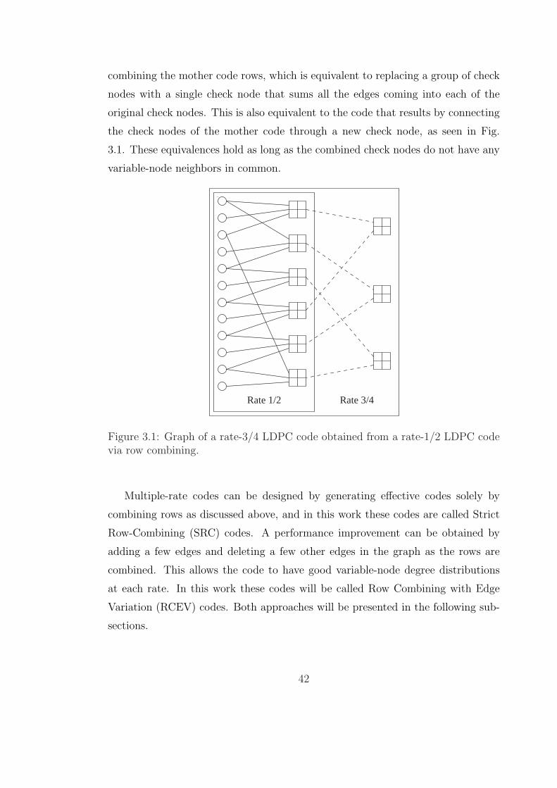
combining the mother code rows, which is equivalent to replacing a group of check
nodes with a single check node that sums all the edges coming into each of the
original check nodes. This is also equivalent to the code that results by connecting
the check nodes of the mother code through a new check node, as seen in Fig.
3.1. These equivalences hold as long as the combined check nodes do not have any
variable-node neighbors in common.
Rate 3/4Rate 1/2
Figure 3.1: Graph of a rate-3/4 LDPC code obtained from a rate-1/2 LDPC codevia row combining.
Multiple-rate codes can be designed by generating effective codes solely by
combining rows as discussed above, and in this work these codes are called Strict
Row-Combining (SRC) codes. A performance improvement can be obtained by
adding a few edges and deleting a few other edges in the graph as the rows are
combined. This allows the code to have good variable-node degree distributions
at each rate. In this work these codes will be called Row Combining with Edge
Variation (RCEV) codes. Both approaches will be presented in the following sub-
sections.
42
Section 3.1 describes the row-combining approach in detail. Section 3.2 explains
how row combining helps to simplify decoder architectures and consequently to
reduce chip area. Section 3.3 describes how to lower the complexity of the encoder
and decoder of row-combining codes. A design method for SRC codes is proposed
in Section 3.4. Section 3.5 describes the RCEV code design approach that results
in an improvement in performance by relaxing some constraints imposed in the
SRC design. Section 3.6 compares the performance of SRC, RCEV, single-rate
stand-alone codes, and punctured codes. Section 3.7 delivers the conclusions of
this chapter.
3.1 Row-Combining Codes
Consider the example mother LDPC matrix in (3.1),
H 12
=
1 1 1 0 0 0 0 0 0 0 0 0
1 0 0 1 1 0 0 0 0 0 0 0
0 0 0 0 1 1 1 0 0 0 0 0
0 0 0 0 0 0 1 1 1 0 0 0
0 0 0 0 0 0 0 0 1 1 1 0
0 0 1 0 0 0 0 0 0 0 1 1
. (3.1)
This is a rate-1/2 mother LDPC matrix with blocklength 12 whose graph repre-
sentation can be seen in Fig. 3.1. This is by no means a good LDPC code but the
reader should see it as an example to explain row combining. Fig. 3.1 also shows
that replacing each pair of nodes with a new single node transforms this rate-1/2
code into a rate-3/4 code. This is equivalent to summing the rows of the mother
LDPC matrix that correspond to the check nodes that are combined, since the
check nodes in the example do not have any common neighbors. In general, the
mother matrix should be designed so that the rows that will be combined don’t
have ones in the same column.
Eq. (3.2) gives the effective rate-3/4 LDPC matrix that results from the row
43
combining described in Fig. 3.1, where combining rows 1 and 4 of the mother
matrix produces row 1 of the effective matrix, combining rows 2 and 5 of the
mother matrix produces row 2 of the effective matrix, and combining rows 3 and
6 of the mother matrix produces row 3 of the effective matrix,
H 34
=
1 1 1 0 0 0 1 1 1 0 0 0
1 0 0 1 1 0 0 0 1 1 1 0
0 0 1 0 1 1 1 0 0 0 1 1
. (3.2)
It is easy to see that many different rates can be obtained from the same mother
code by changing the way rows are combined. For example using the mother code
described in (3.1), combining three rows at a time generates the rate-5/6 LDPC
matrix shown in (3.3). In this rate-5/6 matrix the first row results from combining
the odd rows of the mother matrix and the second row results from combining the
even rows of the mother matrix,
H 56
=
(1 1 1 0 1 1 1 0 1 1 1 0
1 0 1 1 1 0 1 1 1 0 1 1
). (3.3)
In general, row combining changes the rate without changing the blocklength
or the basic architecture of the decoder.
3.2 Impact of Row Combining on the Hardware
Architecture
The main goal of row-combining is to simplify the support of multiple rates. In
general, row-combining won’t lead to a faster decoder for any particular rate but
provides a simple overall architecture with a smaller chip area required to support
all the needed rates. Here are a couple of examples of how decoder simplification
might be accomplished in the case of digital decoders.
If the message passing is done through a memory, there is a list of memory
44
addresses that tell the processor which variable-to-check messages to compute in
order to compute a check-to-variable message. With row-combining, changing the
rate of the code can be achieved by replacing the lists for the combined check nodes
with a single list that is the union of those lists, thus changing only the quantity of
messages read. This is a simple change that can be done on the fly with a careful
implementation.
Another possible hardware implementation can be developed using the fact
that the code produced by row combining is equivalent to the code that results
from connecting the check nodes through another check node as shown in Fig.
3.1. An efficient hardware implementation would decode the higher rate code by
performing the extra-message generation on top of the message computing done
for the low rate codes, thus maintaining the basic hardware architecture. This idea
was used in [33], where an architecture that exploits our row-combining structure
was implemented. These examples, while not exhaustive, capture the essence of
the simplification facilitated by row combining.
On top of these simplified multiple-rate decoders, the fact that the codes are
designed such that the check nodes that will be combined don’t have any neigh-
bors in common guarantees some degree of parallelism. Check nodes that will be
combined can be processed in parallel because they will never try to access the
information of the same variable node. There are, of course, many ways to achieve
parallelism. Our point here is that row combining is completely compatible with
LDPC codes that support highly parallel decoding architectures.
Also, row-combining codes allow programmable analog decoders. An analog
decoder that works for all the rates would consist of the circuit that decodes the
mother code, with switches that turn on and off the connections to the new check
nodes that increase the rate of the code. These connections are shown in Fig. 3.1
with dashed lines.
45
3.3 Structured Row-Combining Codes
The challenge presented when trying to design a structured row-combining code
is that the mother code (denoted by M) and all the effective codes (denoted by
E) must have both the sub-matrix structure (for parallel decoding) and a lower
There is an easy way to maintain the sub-matrix structure for all the effective
codes. Instead of combining individual rows, rows of sub-matrices will be combined
so that if sub-matrix A and sub-matrix B are combined it implies that row i of A
and row i of B will be combined for i = {1, ..., p}. The resulting sub-matrix will
be equivalent to the superposition of sub-matrix A and sub-matrix B.
If the exact sub-matrix structure of [30] is to be maintained for all the effective
codes, the mother code and all effective codes have to be designed so that among the
combined sub-matrices at most only one is non-zero (and has the Si structure).
However, if the sub-matrix that results from the superposition of two or more
non-zero Si sub-matrices also has good parallel properties (which depends on the
hardware architecture of the decoder), this design criteria can be relaxed to include
such superpositions.
Furthermore, it’s desirable that the square H2 sub-matrices of both the mother
code and all effective codes have a lower triangular structure that would allow
back-substitution encoding. This is achieved by imposing a constraint in selection
of the rows to be combined, assuming that the H2 sub-matrix of the mother code
is lower triangular. Let us assume that row-combining generates an effective code
Ei that has ri check-nodes. As long as the bottom ri rows of the mother code
remain in their pre-row-combining relative positions and are not combined among
themselves, the square H2 sub-matrix (with size ri) of the effective code Ei is
lower triangular. The examples presented in Section 3.1 satisfy this condition.
The size-6 square H2 sub-matrix of the rate-1/2 mother LDPC matrix shown in
(refeq:h12) is lower triangular. The effective rate-3/4 code has ri = 3 check-nodes
and the combining is performed so that the bottom 3 rows are not combined among
themselves and remain in their pre-row-combining relative positions. It can be seen
46
in (3.2) that the size-3 square H2 sub-matrix of the effective rate-3/4 code is also
lower triangular.
One way to combine the sub-matrix structure with the lower triangular struc-
ture of H2 is to make H2 block lower triangular. This implies that the sub-matrices
along the diagonal of H2 will have the Si structure and all the sub-matrices that
are above this diagonal will be zero sub-matrices. The problem with this structure
is that the rightmost p columns (where p is the size of the sub-matrices) will be
degree-one columns which will negatively affect the performance of the codes. One
possible solution of the problem is to make the bottom right matrix have the bi-
diagonal structure described in (3.4). This structure allows back-substitution and
only 1 column will have degree 1,
Ss =
1 0 0 0
1 1 0 0
0 1 1 0
0 0 1 1
. (3.4)
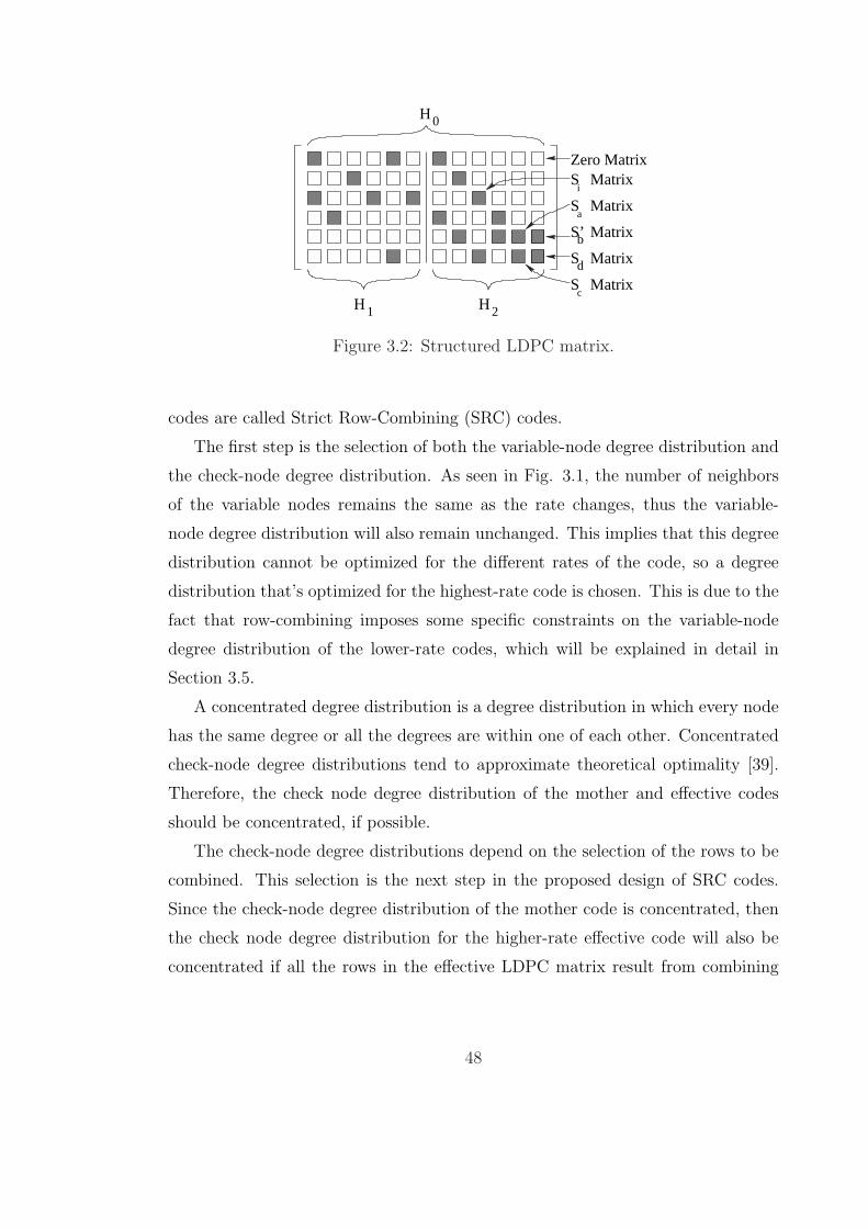
Another solution can be seen in Fig. 3.2 which shows a LDPC structure that al-
lows both parallel decoding and low-complexity encoding. In this structure the four
bottom right matrices are carefully designed such that they allow back-substitution
encoding. For the Si sub-matrices with subscripts i = a, b, c, d, the subscripts (num-
ber of columns shifted) must satisfy (a− c + d− b) mod p = 1. The sub-matrix
labelled S ′b is an Si sub-matrix with the first row set to all zeros. This structure
guarantees that the last 2p parity bits can be generated by solving one parity check
equation with one unknown bit, thus allowing back substitution. In this structure
only 1 column has degree 1.
3.4 Design of Structured SRC Codes
This section proposes a design method for structured row-combining codes given
the blocklength of the code, the mother and effective rates and the sub-block size
p. Since only row combining is allowed to generate the high-rate matrices, these
47
d
b
a
Sc
Matrix
MatrixS
MatrixS’
S Matrix
Zero Matrix
2H
0H
Si
Matrix
1H
Figure 3.2: Structured LDPC matrix.
codes are called Strict Row-Combining (SRC) codes.
The first step is the selection of both the variable-node degree distribution and
the check-node degree distribution. As seen in Fig. 3.1, the number of neighbors
of the variable nodes remains the same as the rate changes, thus the variable-
node degree distribution will also remain unchanged. This implies that this degree
distribution cannot be optimized for the different rates of the code, so a degree
distribution that’s optimized for the highest-rate code is chosen. This is due to the
fact that row-combining imposes some specific constraints on the variable-node
degree distribution of the lower-rate codes, which will be explained in detail in
Section 3.5.
A concentrated degree distribution is a degree distribution in which every node
has the same degree or all the degrees are within one of each other. Concentrated
check-node degree distributions tend to approximate theoretical optimality [39].
Therefore, the check node degree distribution of the mother and effective codes
should be concentrated, if possible.
The check-node degree distributions depend on the selection of the rows to be
combined. This selection is the next step in the proposed design of SRC codes.
Since the check-node degree distribution of the mother code is concentrated, then
the check node degree distribution for the higher-rate effective code will also be
concentrated if all the rows in the effective LDPC matrix result from combining
48
the same number of rows of the mother LDPC matrix. It is also necessary that
the row combining maintains the structure of the codes presented in Section 3.3.
There is a simple way to achieve this if the desired rates have the (a − 1)/a
form. The mother code is set to have a square matrix with a concentrated check
node degree distribution. Such a mother code has rate 0 and is used only to
generate effective codes; it is not a useful stand alone code. Combining a rows (or
rows of sub-matrices in the case of structured codes) at a time, generates a code
with rate (a − 1)/a as long as the total number of rows of the mother matrix is
a multiple of a. This effective code will have a concentrated check node degree
distribution. This shows that SRC codes can maintain a concentrated check node
degree distribution among all its rates if they all are in the (a− 1)/a form. Rates
of this form comprise a useful set of rates. In standards such as IEEE 802.11n, all
LDPC code rates have this form. Furthermore, puncturing and/or shortening can
be used with row combining in order to support more rates. As long as the number
of punctured and/or shortened bits is small, the effective blocklength of the code
is not significantly diminished.
Given that two check nodes that will be combined cannot have any common
neighbors, row combining introduces some constraints in the construction of the
LDPC matrices. These constraints may limit the degrees of freedom of the LDPC
design, especially in the case of structured LDPC codes where two sub-matrices
that will be combined can’t be both non-zero. In order to minimize this problem,
the overall number of row combinations across all rates must be as low as possi-
ble. This can be achieved by first choosing the row combining that generates the
highest-rate code. Once this is done, the row-combining that generates the second
highest rate-code is chosen using as many row combinations from the highest rate-
code as possible. If all the row-combining strategies are chosen this way the overall
number of combinations will be minimized. This minimization of the number of
combinations is also beneficial from an implementation point of view.
The remaining issue is to assign the positions and right cyclic shifts of the non-
zero sub-matrices in the mother code. It is well known that the performance of the
LDPC codes is limited by the fact that their graphs contain cycles which compro-
49
mise the optimality of the belief propagation decoding. These cycles generate error
floors in the performance of LDPC codes in the high SNR regions. However, the
negative effect of the cycles can be reduced using graph-conditioning techniques
such as those described in [41] and [42]. So the last step in the design will be to
use the ideas described in these works, adapting them to work on structured SRC
codes.
As explained in [41] not all cycles degrade the performance of the code in the
same way. Among the most dangerous structures that can be found in LDPC
bi-partite graphs are stopping sets. A stopping set is a variable node set where all
its neighbors are connected to the set at least twice. This implies that if all the
variable nodes that belong to a stopping set are unreliable, the decoding will fail.
Small stopping sets must be avoided. This is a complex problem to attack
directly. To indirectly increase the size of stopping sets, [41] proposes the ACE
algorithm, which is based on maximizing the ACE metric of small cycles. The
ACE metric of a cycle is the sum of the number of neighbors of each of the variable
nodes in the cycle minus two times the number of variable nodes in the cycle.
According to this algorithm, the LDPC matrix is constructed by generating
a single column randomly until one is found where all the cycles of length less
than or equal to a previously specified threshold (denoted as 2dACE) that contain
its corresponding variable node have an ACE metric higher than or equal to an-
other previously specified threshold (denoted as ηACE). This process sequentially
produces all the columns starting from the one with the lowest degree.
The constraints specified in [42] also help to avoid small stopping sets in the
graph, particularly if applied to the high-degree columns. In [42] two new metrics
are defined called βc and βp and they are the number check nodes connected only
once to a cycle or a path respectively. In the same manner as the ACE algorithm,
random columns are generated and they must satisfy some constraints based on
previously specified thresholds which are denoted here as dSS, γc and γp. Specif-
ically, a randomly generated column is valid if all the cycles of length less than
or equal to 2dSS that contain its corresponding variable node have a βc metric of
value higher than or equal to γc and if all the paths of length less than or equal to
50
dSS that contain its corresponding variable node have a βp metric of value higher
than or equal to γp.
The generation of the mother and effective matrices is done using simulta-
neous graph conditioning. This means that the previously described column by
column generation is still used and every column generated must satisfy the graph
constraints specified for the mother code and all the effective codes. Different
graph constraints can be used for different matrices, which is necessary because
the achievable values of these constraints change with the rate as shown in [56].
In the case of structured SRC codes, instead of a column by column generation,
all the columns that correspond to the same sub-matrices will be generated at the
same time.
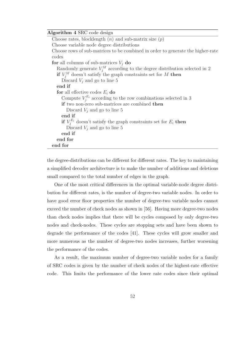
The design procedure of structured SRC codes is shown in Algorithm 4 where Vj
denotes a set of variable nodes that belong to a sub-matrix, V Mj denotes a column
of sub-matrices in the mother code M and V Eij denotes a column of sub-matrices
in the effective code Ei. Algorithm 4 may not converge because the conditions
are too restrictive. In that case, we can relax the graph-constraints by lowering
the values of dACE, ηACE, dSS, γc, and/or γp. However, even if there aren’t any
graph-constraints, Algorithm 4 may not converge because there may be too many
effective rates that impose too many constraints thus the number of effective-rates
must be lowered.
3.5 Row Combining with Edge Variation (RCEV)
Codes
The main disadvantage with SRC codes is that the mother code and all of the effec-
tive codes of an SRC code have the same variable-node degree distribution. With
strict row combining, edges are neither created nor deleted. This is problematic
since in principle different rates require different variable-node degree distributions
for theoretical optimality, as stated in [39]. Row combining with edge variation
(RCEV) codes allow the addition and deletion of edges as rows are combined so
51
Algorithm 4 SRC code design
Choose rates, blocklength (n) and sub-matrix size (p)Choose variable node degree distributionsChoose rows of sub-matrices to be combined in order to generate the higher-ratecodesfor all columns of sub-matrices Vj do
Randomly generate V Mj according to the degree distribution selected in 2
if V Mj doesn’t satisfy the graph constraints set for M then
Discard Vj and go to line 5end iffor all effective codes Ei do
Compute V Eij according to the row combinations selected in 3
if two non-zero sub-matrices are combined thenDiscard Vj and go to line 5
end ifif V Ei
j doesn’t satisfy the graph constraints set for Ei thenDiscard Vj and go to line 5
end ifend for
end for
the degree-distributions can be different for different rates. The key to maintaining
a simplified decoder architecture is to make the number of additions and deletions
small compared to the total number of edges in the graph.
One of the most critical differences in the optimal variable-node degree distri-
bution for different rates, is the number of degree-two variable nodes. In order to
have good error floor properties the number of degree-two variable nodes cannot
exceed the number of check nodes as shown in [56]. Having more degree-two nodes
than check nodes implies that there will be cycles composed by only degree-two
nodes and check-nodes. These cycles are stopping sets and have been shown to
degrade the performance of the codes [41]. These cycles will grow smaller and
more numerous as the number of degree-two nodes increases, further worsening
the performance of the codes.
As a result, the maximum number of degree-two variable nodes for a family
of SRC codes is given by the number of check nodes of the highest-rate effective
code. This limits the performance of the lower rate codes since their optimal
52
degree-distribution generally requires a significantly larger number of degree-two
variable nodes [39]. The difference in the distributions depends on the rates of both
the mother code and all the effective codes. The loss in performance due to this
limitation increases as the range of possible rates of the SRC codes grows larger.
In order to avoid this problem in RCEV codes, the number of degree-two vari-
able nodes in the mother code is set to be the optimal for the lowest-rate code.
For high-rate effective codes, edges are added to some degree-two variable nodes so
that the maximum number of degree-two nodes is less than or equal to the number
of check nodes in the graph. Therefore, when generating the effective code Ei,
there is a set of degree-two variable nodes (SEi) that have degree 3 in the code Ei.
This, unfortunately, is not the only problem generated by the common degree-
distribution. Layered Belief Propagation (LBP), a decoding method that improves
the convergence speed and allows a low complexity hardware architecture, was
introduced in [24] and [26]. LBP decoding requires the parity-check matrix to be
divided into sub-matrices that can have at most one “1” per column and one “1”
per row. Thus, in order to generate an LDPC code that can be decoded with LBP,
the maximum variable-node degree is the number of sub-matrices in a column,
which is the number check nodes divided by the size of the sub-matrices. For
SRC codes that support LBP, the maximum variable-node degree must be the
same for all rates, and it is given by the number of check nodes of the highest
rate code divided by the size of the sub-matrices. As stated in [39], increasing
the maximum variable-node degree results in a better code. The SRC common
degree-distribution imposes a strict limit on the maximum variable-node degree,
and thus a performance limit when LBP decoding is used.
The technique used in RCEV codes to avoid this problem is the following. If
during the row combining, a non-zero sub-matrix is added to another non-zero
sub-matrix, one of them is discarded in order maintain the structure mentioned
before. This allows RCEV codes to have different maximum variable-node degrees
for different rates which will improve the performance of the lower rate codes.
RCEV codes are designed using the steps for SRC codes given in Section 3.4,
along with the edge variation techniques described in this section as shown in
53
Algorithm 5.
Algorithm 5 RCEV code design
1: Choose rates, blocklength (n) and sub-matrix size (p)2: Choose variable node degree distributions3: Choose the variable-node sets SCi
4: Choose rows of sub-matrices to be combined in order to generate the higher-rate codes
5: for all columns of sub-matrices Vj do6: Randomly generate V M
j according to the degree distribution of the lowest-rate code
7: if V Mj doesn’t satisfy the graph constraints set for M then
8: Discard Vj and go to line 69: end if
10: for all effective codes Ei do11: Compute V Ei
j according to the row combinations selected in 412: if two non-zero sub-matrices are combined then13: if The degree of V M
j is less than maximum variable-node degree then14: Discard Vj and go to line 615: else16: Discard one of the non-zero sub-matrices17: end if18: end if19: if V Ei
j doesn’t satisfy the graph constraints set for Ei then20: Discard Vj and go to line 621: end if22: if Vj ∈ SEi then23: randomly add a non-zero sub-matrix to V Ei
j
24: end if25: end for26: end for
3.6 Performance Comparison
The following figures show the performance of row-combining codes, designed using
all the techniques presented above, on the AWGN channel with a flooding LDPC
decoder. Fig. 3.3 shows the performance of a structured SRC code family and the
corresponding four stand-alone codes selected for the IEEE 802.11n standard [48].
54
1 1.5 2 2.5 3 3.5 4 4.510
−4
10−3
10−2
10−1
100
Eb/N
o
FE
R
1/22/33/45/6SRC802.11n
Figure 3.3: Performance of structured SRC with p=27 and IEEE 802.11n codeswith blocklength 1944 on an AWGN channel. Maximum number of iterations equalto 15.
The specifications of the structured SRC code family are the following. The mother
code has rate 0, while the four effective codes have rates 1/2, 2/3, 3/4, and 5/6.
The blocklength of the codes is 1944 bits, the size of the sub-matrices is 27x27,
a maximum of 15 iterations was used in the simulation. It has at most one “1”
per column and one “1” per row given and therefore allows the simplified decoder
proposed in [24].
Fig. 3.3 shows that the SRC codes perform very well under these conditions
(blocklength, sub-matrix size, and number of iterations). The sub-matrix size is
small enough to allow a sufficiently large maximum variable-node degree. The
effect of the non-optimality of the variable-node degree distribution for the rate-
1/2 code is small for 15 iterations. This is because for such a small number of
iterations performance is dominated by the high-degree variable nodes. Thus,
the lower-than-optimal number of degree-two nodes of the rate-1/2 code does not
dramatically affect performance. For fifty iterations, the rate-1/2 code performance
55
Table 3.1: Variable-node degree distributions of structured SRC and RCEV codes.
This comparison at 15 iterations is practically important since there are many
applications that only allow a small number of iterations of the decoder. For
example, in most wireless applications the channel decoding must be done in a very
small amount of time, which limits the maximum number of iterations allowed.
Fig. 3.4 presents another comparison of the performance of a structured SRC
code, the four stand-alone codes selected for the IEEE 802.11n standard, and a
structured RCEV code. The row-combining codes have a mother code with rate 0,
while the four effective codes have rates 1/2, 2/3, 3/4, and 5/6. The variable-node
degree distribution of both codes can be found in Table 3.1. The blocklength of
the codes is 1944 bits, the size of the sub-matrices of the row-combining codes is
54x54 and a maximum of 50 iterations was used in these simulations. SRC and
RCEV codes of the same rate have similar total number of edges. The maximum
difference, found in the rate-3/4 code, is a 7%.
As expected, Fig. 3.4 shows the loss in performance of the SRC low rate codes.
The SRC rate-1/2 code show a performance loss of more than 0.2 dB with respect
to the IEEE 802.11n codes with the same blocklength and this is due to their
inadequate variable-node degree distribution.
As observed in Fig. 3.4 the FER of the lower rates of the RCEV code are
significantly better than those of the lower rates of the SRC code. This gain
follows from the improved degree distributions of the RCEV codes over those of
the SRC codes. The magnitude of the difference between the degree distributions
of the rate-1/2 codes can be seen in Table 3.1. For the high rate codes there is very
56
1 1.5 2 2.5 3 3.5 410
−4
10−3
10−2
10−1
100
Eb/N
o
FE
R
1/22/33/45/6SRC802.11nRCEV
Figure 3.4: Performance of structured SRC with p=54, structured RCEV, andIEEE 802.11n codes with blocklength 1944 on an AWGN channel. Maximumnumber of iterations equal to 50.
57
Table 3.2: Graph-conditioning constraints of structured SRC and RCEV codes.
little difference between the performances of the RCEV and SRC codes, since their
degree distributions are very similar. RCEV techniques allow the optimization of
the degree distributions for each rate.
Fig. 3.4 also shows that the RCEV codes perform close to the IEEE 802.11n
codes. As expected there is a small loss due to the fact that RCEV codes must
satisfy the row-combining constraints. This slightly reduces the degrees of freedom
during the design process, thus making the set of all the possible RCEV codes a
subset of all the possible stand-alone codes. Table 3.2 shows the graph-conditioning
constraints used to generate these row-combining codes.
As mentioned before, the row-combining codes presented in this section have a
rate-0 mother code. We previously designed codes that had a rate-1/2 mother code
with the same variable-node degree distribution [57]. This mother code forces the
effective rate-2/3 code to have a non-concentrated check-node degree distribution.
This translates into a 0.3 dB loss at a FER of 10−3 in the performance of the rate-
2/3 code when compared to the 802.11n rate 2/3 code. Having a rate-0 mother
code reduces the loss to 0.1 dB as shown in Fig. 3.3.
A comparison in the performance of RCEV codes and punctured LDPC codes is
shown in Fig. 3.5. The punctured codes correspond to the ones presented in [55].
The RCEV code was designed to have very similar degree distributions to the
punctured codes so that the comparison would be fair. The blocklength of the
mother code of the punctured codes is 1024 while the blocklength of the RCEV
codes is 1030. There is a clear performance gap between the higher rate codes.
This is due to the fact that puncturing reduces the effective blocklength of the
58
1 2 3 4 5 610
−5
10−4
10−3
10−2
10−1
100
Eb/N
o
FE
R
1/24/59/10PunctRCEV
Figure 3.5: Performance of RCEV codes and punctured LDPC codes.
code.
Sphere-packing bounds [58] give a lower bound on the SNR that can support
reliable communication as a function of blocklength. The gap between the sphere-
packing bounds of several rate-9/10 row-combining code and rate-9/10 punctured
codes with equal mother-code blocklength (based on the different blocklengths) can
be seen in Fig. 3.6. The loss in performance of the punctured codes decreases as the
mother-code blocklength increases. However, the theoretical gap at a blocklength
of 1030 is half of the performance gap shown in Fig. 3.5. That punctured codes
aren’t always the best codes for their effective blocklength may help to explain why
there is a bigger gap in the actual performance of the codes.
3.7 Conclusions
As we know from information theory, channel codes approach capacity-achieving
performance as blocklength goes to infinity. Both theory and practice confirm
59
0 2000 4000 6000 8000 10000 120000.06
0.08
0.1
0.12
0.14
0.16
0.18
0.2
0.22
0.24
Blocklength of mother matrix
Per
form
ance
gap
(dB
)
Figure 3.6: Sphere-packing bound gap at a FER of 10−3 between row-combiningcodes and punctured codes. Both codes have the same rate (9/10) and have equalmother-code blocklength. The mother code of the punctured codes has rate 1/2.
60
that codes with longer blocklengths perform better. Recently, puncturing and
shortening have been used to provide a variety of rates in the context of a single
decoder architecture, but these techniques shorten the code blocklength as rates
move away from the rate of the mother code.
Multiple-rate LDPC codes that avoid this blocklength reduction can be gener-
ated using a row-combining approach. Structures that reduce complexity of both
encoder and decoder can be applied and maintained through all the rates, and
graph conditioning algorithms can be applied to the design of the codes to produce
good error floor performances at all the rates.
Structured SRC codes allow the use of simple hardware architectures (or pro-
grammable analog-decoding circuits) that can be used to decode the mother and all
the effective rates. The design of these codes imposes some constraints that barely
affect the performance when the codes are used at a small number of iterations. As
the maximum number of iterations increases, the performance gap between SRC
codes and stand-alone codes also increases.
RCEV codes relax the constraints required for SRC codes, and show a gain in
performance with respect to SRC codes for a large number of iterations. This in-
crease in performance comes at a cost of architecture complexity. The performance
of RCEV codes is very close to the performance of stand-alone codes for a large
number of iterations.
These codes become attractive for applications that require both performance
close to capacity and a low decoder complexity due to the fact that RCEV codes
have still a strong inherent structure that can be exploited in the hardware de-
coder.
61
Chapter 4
Conclusions
This dissertation presents novel techniques that can result in better LDPC de-
coders. On one hand, dynamic scheduling can improve the error-rate performance
of an LDPC decoder. A decoder able to implement IDS can outperform rival de-
coders working on the same standardized code. On the other hand, CBMR code
design leads to families of codes that can re-use the same decoding hardware thus
reducing the decoder complexity for multiple-rate systems.
There are still several challenges to be addressed. It was shown intuitively
and heuristically that IDS solves some trapping-set errors. The percentage of
solved trapping-set errors continues to be an open problem. Furthermore, trapping-
set errors were introduce to explain the error-floor behavior of LDPC codes, a
careful study of the IDS behavior in the error-floor region is needed. We proposed
parameterized Mixed-IDS strategies that could be carefully studied in order to
obtain optimal theoretical values of their parameters ζ and ξ.
A quantification of the advantages of both IDS and CBMR codes is needed.
The trade-off provided by IDS between increasing the per-iteration complexity and
reducing the number of iterations (while also reducing the FER for a large number
of iterations) requires further investigation in the context of specific implementa-
tions. Future work could compare the difference between the actual throughput,
area, and power consumption of different scheduling strategies. A specific challenge
in the implementation of IDS is to solve the memory clash problem present in P-
62
ANS. The practical benefits of CBMR, in both digital and analog implementations,
should also be quantized.
The scheduling ideas presented in this work may be extended to other commu-
nication solutions that use iterative BP, such as turbo codes, turbo-equalization,
iterative demodulation and decoding of high-order constellations, among others.
The extensions of the IDS strategies may also prove beneficial for loopy-BP solu-
tions to problems outside the communications field.
63
Bibliography
[1] R. Hamming. Error detecting and error correcting codes. Bell Syst. Tech. J.,
29:147–160, Apr 1950.
[2] C. E. Shannon. A mathematical theory of communication. Bell Syst. Tech.
J., 27:379–423 and 623–656, July and Oct. 1948.
[3] I.S. Reed. A class of multiple-error correcting codes and their decoding scheme.
IRE Trans. Inform. Theory, (4):38–42, 1954.
[4] D.E. Muller. Application of boolean algebra to switching circuit design and
to error detection. IRE Trans. Electron. Computers, (3):6–12, 1954.
[5] P. Elias. Coding for noisy channels. IRE Convention Record, (4):37–46, Mar
1955.
[6] A. Hocquenghem. Codes correcteurs derreurs. Chiffres, 2:147–156, Sep 1959.
[7] R.C. Bose and D.K. Ray-chaudhuri. On a class of error-correcting binary
group codes. Inform. Contr., 3:68–79, 1960.
[8] I. Reed and G. Solomon. Polynomial codes over certain finite fields. SIAM
Journal of Applied Mathematics, 8:300–304, 1960.
[9] G. Ungerboeck. Channel coding with multilevel/phase signals. IEEE Trans.
on Inform. Theory, 25:55–67, 1982.
[10] E. Berlekamp. Algebraic Coding Theory. New York: McGraw-Hill, 19618.
64
[11] J. Massey. Shift-register synthesis and bch decoding. IEEE Trans. on Inform.
Theory, 15:122–127, 1969.
[12] R. Hamming. Error bounds for convolutional codes and an asymptotically
optimal decoding algorith. IEEE Transactions on Information Processing,
13:260–269, Apr 1967.
[13] J.M. Wozencraft and B. Reiffen. Sequential Decoding. Cambridge, MA: MIT
Press, 1961.
[14] C. Berrou, A. Glavieux, and P. Thitimajshima. Near Shannon limit error-
correcting coding and decoding: Turbo codes. Proc. IEEE Int. Conf. on
Comm. (ICC), pages 1064–1070, May 1993.
[15] F. Kschischang, B. J. R. Frey, and H.-A. Loeliger. Factor graphs and the sum-
product algorithm. IEEE Trans. on Inform. Theory, 47(2):498–519, March
2001.
[16] R.E. Blahut. Theory and Practice of Error Control Codes. Addison-Wesley,
1983.
[17] E.R. Berlekamp, R.J. McEliece, and H.C.A. Van Tilborg. On the inherent
intractability of certain coding problems. IEEE Trans. on Inform. Theory,
24:384–386, May 1978.
[18] R. G. Gallager. Low-density parity-check codes. IRE Trans. Inform. Theory,
IT-8:21–28, Jan. 1962.
[19] D.J.C. MacKay and R.M. Neal. Near shannon limit performance of low-density
parity-check codes. Electronics Letters, 32:1645–1646, Aug 1996.
[20] J. Pearl. Probabilistic Reasoning in Intelligent Systems: Networks of Plausible
Inference. Morgan Kaufmann, 1988.
65
[21] R.J. McEliece, D.J.C. MacKay, and Jung-Fu Cheng. Turbo decoding as an
instance of Pearl’s “belief propagation” algorithm. IEEE Journal on Selected
Areas in Communications, 16:140–152, February 1998.
[22] N. Wiberg. Codes and decoding on general graphs. Ph.D. Dissertation, De-
partment of Electrical Engineering, Linkoping University, Linkoping, Sweden.
1996.
[23] M. Fossorier, M. Mihaljevic, and H. Imai. Reduced complexity iterative de-
coding of low density parity check codes based on belief propagation. IEEE
Trans. on Comm., 47:673–680, May 1999.
[24] M.M. Mansour and N.R. Shanbhag. High-throughput LDPC decoders. IEEE
Trans. Very Large Scale Integration (VLSI) Systems, 11:976–996, December
2003.
[25] H. Kfir and I. Kanter. Parallel versus sequential updating for belief propaga-
tion decoding. Physica A, 330:259–270, 2003.
[26] D. Hocevar. A reduced complexity decoder architechture via layered decoding
of LDPC codes. In Proc. Signal Processing Systems SIPS 2004, pages 107–112,
October 2004.
[27] E. Sharon, S. Litsyn, and J. Goldberger. An efficient message-passing sched-
ule for LDPC decoding. In Proc. 23rd IEEE Convention of Electrical and
Electronics Engineers in Israel, pages 223–226, September 2004.
[28] J. Zhang and M. Fossorier. Shuffled belief propagation decoding. IEEE Trans.
on Comm., 53:209–213, February 2005.
[29] P. Radosavljevic, A. de Baynast, and J.R. Cavallaro. Optimized message pass-
ing schedules for LDPC decoding. In Proc. Thirty-Ninth Asilomar Conference
on Signals, Systems and Computers, pages 591–595, 2005.
66
[30] M. M. Mansour and N. R. Shanbhag. Low Power VLSI Decoder Architectures
for LDPCCs. 2002 International Low Power Electronics and Design, pages .
284–289, June 2002.
[31] Mustafa Eroz, Feng-Wen Sun, and Lin-Nan Lee. An Innovative Low-Density
Parity-Check Code Design With Near-Shannon-Limit Performance and Simple
Implementation. IEEE Trans. on Comm., 54(1), January 2006.
[32] V. Novichkov, H.Jin, and T. Richardson. Programmable vector processor
architecture for irregular LDPC codes. In Proc. Conf. on Inform. Systems
and Sciences, pages . 1141–1146, Princeton, NJ, March 2004.
[33] M. Rovini, N. E. L’Insalata, F. Rossi, and L. Fanucci. VLSI Design of High-
Throughput Multi-Rate Decoder for Structured LDPC Codes. In Proc. 8th
Euromicro Conference on Digital System Design, Porto, Portugal, August
2005.
[34] J. Hagenauer. Decoding of binary codes with analog networks. In Proc. 1998
Information Theory Workshop, pages 13–14, San Diego, CA, February 1998.
[35] H.-A. Loeliger, F. Lustenberger, M. Helfenstein, and F. Tarkoy. Probability
propagation and decoding in analog VLSI. In Proc. 1998 IEEE Int. Symp.
Inform. Th., page 146, Cambridge, MA, August 1998.
[36] F. Lustenberger. On the Design of Analog VLSI Iterative Decoders. PhD
thesis, Diss. ETH No 13879, November 2000.
[37] M. Yang, W. E. Ryan, and Y. Li. Design of Efficiently Encodable Moderate-
LengthHigh-Rate Irregular LDPC Codes. IEEE Trans. on Comm., 52(4):564–
571, April 2004.
[38] T. Richardson and R. Urbanke. Efficient encoding of low-density parity-check
codes. IEEE Trans. Inform. Theory, 47:638–656, February 2001.
67
[39] T. Richardson, A. Shokrollahi, and R. Urbanke. Design of capacity-