Article

Improving MMS Performance during InfrastructureSurveys through Geometry Aided Design

Conor Cahalane 1,*,†, Paul Lewis 1, Conor P. McElhinney 2, Eimear McNerney 3

and Tim McCarthy 1

1 National Centre for Geocomputation, Maynooth University, Co. Kildare, Ireland;paul.lewis@nuim.ie (P.L.); tim.mccarthy@nuim.ie (T.M.)

2 Amazon Data Services, County Dublin, Dublin, Ireland; conormce@cs.nuim.ie3 Electricity Supply Board (ESB), Planning and Asset Management, Group Property, 27 Lower

Fitzwilliam Street, Dublin 2, Ireland; eimear.mcnerney@esb.ie* Correspondence: conor.cahalane@nuim.ie; Tel.: +353-1-7086204† Current address: National Centre for Geocomputation, Iontas, North Campus, Maynooth University,

Maynooth, Co. Kildare, Ireland.

Academic Editors: Lucía Díaz Vilariño and Miguel AzenhaReceived: 2 October 2016; Accepted: 29 November 2016; Published: 8 December 2016

Abstract: A Mobile Mapping System (MMS) equipped with laser scanners can collect large volumes ofLiDAR data in a short time frame and generate complex 3D models of infrastructure. The performanceof the automated algorithms that are developed to extract the infrastructure elements from thepoint clouds and create these models are largely dependent on the number of pulses strikinginfrastructure in these clouds. Mobile Mapping Systems have evolved accordingly, adding more andhigher specification scanners to achieve the required high point density, however an unansweredquestion is whether optimising system configuration can achieve similar improvements at noextra cost. This paper presents an approach for improving MMS performance for infrastructuresurveys through consideration of scanner orientation, scanner position and scanner operatingparameters in a methodology referred to as Geometry Aided Design. A series of tests were designedto measure point cloud characteristics such as point density, point spacing and profile spacing.Three hypothetical MMSs were benchmarked to demonstrate the benefit of Geometry Aided Designfor infrastructure surveys. These tests demonstrate that, with the recommended scanner configuration,a MMS, operating one high specification scanner and one low specification scanner, is capable ofcomparable performance with two high-end systems when benchmarked against a selection of planar,multi-faced and cylindrical targets, resulting in point density improvements in some cases of upto 400%.

Keywords: infrastructure surveys; mobile mapping; LiDAR; point density; performance

1. Introduction

The high volumes of density spatial data produced by Mobile Mappinh Systems (MMSs) [1,2]result in increased processing times. Manual interpretation and extraction of features in the datasetcan be very time consuming, and as a result one of the aims of the research community is todevelop automated extraction of features in the point cloud. These algorithms can potentiallyreduce or eliminate the amount of manual interrogation of the data. Automated algorithms havebeen developed to identify trees, poles, road edges and are an important research question [3–9].However, one important consideration when designing each algorithm is the characteristics of thepoint cloud that will enable successful extraction of a feature. Studies demonstrate [10–12] that aminimum number of laser points and scan profiles are required on cylindrical objects to accurately

Infrastructures 2016, 1, 5; doi:10.3390/infrastructures1010005 www.mdpi.com/journal/infrastructures

Infrastructures 2016, 1, 5 2 of 15

recognise those features and laser point cloud density directly impacts on the accuracy [13] of theresulting extracted model.

Point density is traditionally quoted in points per m2, an unsuitable description for a 3Dimensional (3D) object [14]. This issue has been explored [15] for terrestrial and aerial LiDARand ways to define point density for 3D data and the importance of achieving a sufficient pointdensity on data processing identified. It is difficult to calculate what point density a MMS will becapable of and this paper will further the body of knowledge on MMS performance. MMS surveyspecifications have been created [16,17] to inform surveyors as to what is required from a survey; andrecent publications [18] have improved on this by subdividing point density into coarse, intermediate,and fine point cloud density. Further recommendations are that a continuous, color-coded pointdensity map with summary statistics for the survey area is included as a deliverable. These guidelinesprovide tabular information on what point spacing is required to achieve a specific level of pointdensity, but does not define what MMS hardware, hardware configuration or operating parametersare required to achieve that point spacing. At present there are no generic, robust, easily repeatablemethods for quantifying or assessing the point density exhibited by MMSs.

This paper will apply an existing methodology to quantifying MMS point clouds,thereby improving MMS performance through the following innovative MMS configurations andoperating parameters:

1. Utilising both axes of the MMS for the second scanner to reduce scan range.2. Increasing the length of scan profile that intersects with a target by changing the vertical

orientation of the scanner.3. Limiting the Field of View (FOV) of the scanner to decrease the angular step width between

subsequent laser pulses.

2. Background and Related Work

There are many types of MMS and they are capable of varied performances, and althougha number of studies have explored this in the past, the innovative method proposed in this paperwill allow MMSs to be explored in greater detail, enabling easier, multi-system benchmarking usingnon-default configurations.

2.1. MMS Types

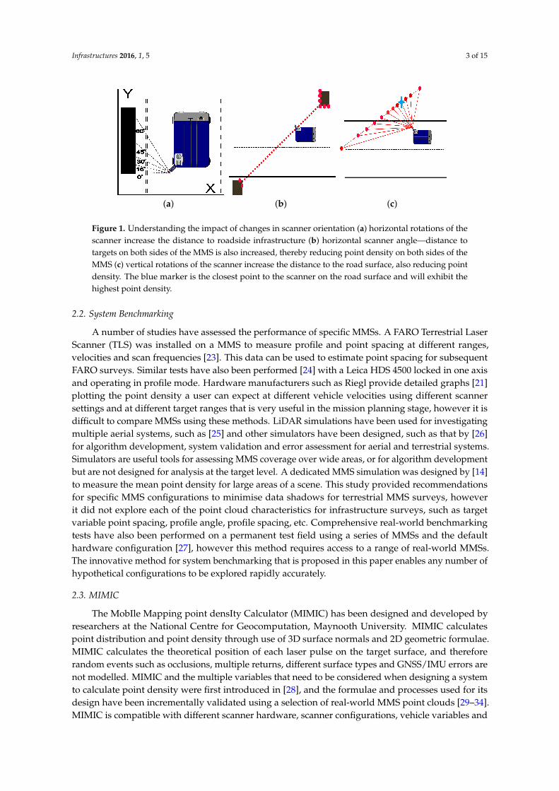
An MMS operating laser scannerz evolved from single scanner systems to the dual scannersystems such as those leading the market today [19–22]. These scanners operate in the ’butterfly’configuration, with the two scanners positioned symmetrically at the rear of the vehicle, angled toeither side of the vehicle. The dual scanner systems on the market incorporate vertical and horizontalrotations of the scanner to ensure that the laser scanner will be capable of surveying structures thatare perpendicular to the direction of travel. These scanner orientations also directly impact the angleat which the scan plane intersects with the surrounding environment and also changes the range tothe target (Figure 1a). Horizontal scanner rotations result in an increased range to the target on bothsides of the vehicle, as displayed in Figure 1b, whereas vertical orientations of the scanner result inan increased range to the road surface underneath the MMS. Incorporating both orientations in bothaxes, horizontal and vertical, results in an increased range to the road surface and also to roadsidetargets, as displayed in Figure 1c. There is therefore a clear need to investigate the influence that scannerorientations have when surveying roadside infrastructure and to identify the optimal configuration.MMS performance analysis and benchmarking enables this.

Infrastructures 2016, 1, 5 3 of 15

(a) (b) (c)

Figure 1. Understanding the impact of changes in scanner orientation (a) horizontal rotations of thescanner increase the distance to roadside infrastructure (b) horizontal scanner angle—distance totargets on both sides of the MMS is also increased, thereby reducing point density on both sides of theMMS (c) vertical rotations of the scanner increase the distance to the road surface, also reducing pointdensity. The blue marker is the closest point to the scanner on the road surface and will exhibit thehighest point density.

2.2. System Benchmarking

A number of studies have assessed the performance of specific MMSs. A FARO Terrestrial LaserScanner (TLS) was installed on a MMS to measure profile and point spacing at different ranges,velocities and scan frequencies [23]. This data can be used to estimate point spacing for subsequentFARO surveys. Similar tests have also been performed [24] with a Leica HDS 4500 locked in one axisand operating in profile mode. Hardware manufacturers such as Riegl provide detailed graphs [21]plotting the point density a user can expect at different vehicle velocities using different scannersettings and at different target ranges that is very useful in the mission planning stage, however it isdifficult to compare MMSs using these methods. LiDAR simulations have been used for investigatingmultiple aerial systems, such as [25] and other simulators have been designed, such as that by [26]for algorithm development, system validation and error assessment for aerial and terrestrial systems.Simulators are useful tools for assessing MMS coverage over wide areas, or for algorithm developmentbut are not designed for analysis at the target level. A dedicated MMS simulation was designed by [14]to measure the mean point density for large areas of a scene. This study provided recommendationsfor specific MMS configurations to minimise data shadows for terrestrial MMS surveys, howeverit did not explore each of the point cloud characteristics for infrastructure surveys, such as targetvariable point spacing, profile angle, profile spacing, etc. Comprehensive real-world benchmarkingtests have also been performed on a permanent test field using a series of MMSs and the defaulthardware configuration [27], however this method requires access to a range of real-world MMSs.The innovative method for system benchmarking that is proposed in this paper enables any number ofhypothetical configurations to be explored rapidly accurately.

2.3. MIMIC

The MobIle Mapping point densIty Calculator (MIMIC) has been designed and developed byresearchers at the National Centre for Geocomputation, Maynooth University. MIMIC calculatespoint distribution and point density through use of 3D surface normals and 2D geometric formulae.MIMIC calculates the theoretical position of each laser pulse on the target surface, and thereforerandom events such as occlusions, multiple returns, different surface types and GNSS/IMU errors arenot modelled. MIMIC and the multiple variables that need to be considered when designing a systemto calculate point density were first introduced in [28], and the formulae and processes used for itsdesign have been incrementally validated using a selection of real-world MMS point clouds [29–34].MIMIC is compatible with different scanner hardware, scanner configurations, vehicle variables and

Infrastructures 2016, 1, 5 4 of 15

target variables and provides detailed information in tabular or graphical format (using interpolationtechniques designed in [35]) to help visualise point and profile distribution.

3. Enabling MMS Performance Improvements through Geometry Aided System Design

MIMIC enables a methodology for benchmarking MMS performance developed at MaynoothUniversity, entitled, Geometry Aided Design (GAD). This paper will use GAD to demonstrate thebenefit of utilising both the X and Y axes of the MMS for scanner position, identifying the optimumvertical orientation of the scanner and assessing the influence of limiting the FOV of the scanner.

3.1. Scanner Position

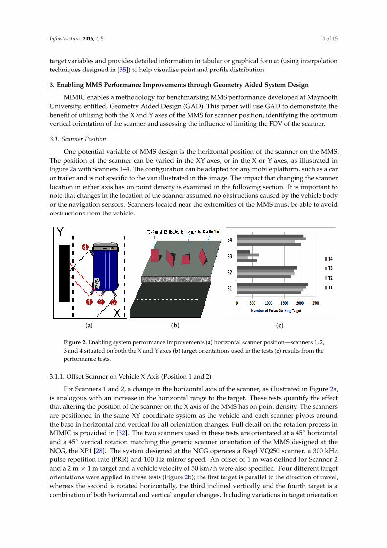
One potential variable of MMS design is the horizontal position of the scanner on the MMS.The position of the scanner can be varied in the XY axes, or in the X or Y axes, as illustrated inFigure 2a with Scanners 1–4. The configuration can be adapted for any mobile platform, such as a caror trailer and is not specific to the van illustrated in this image. The impact that changing the scannerlocation in either axis has on point density is examined in the following section. It is important tonote that changes in the location of the scanner assumed no obstructions caused by the vehicle bodyor the navigation sensors. Scanners located near the extremities of the MMS must be able to avoidobstructions from the vehicle.

(a) (b) (c)

Figure 2. Enabling system performance improvements (a) horizontal scanner position—scanners 1, 2,3 and 4 situated on both the X and Y axes (b) target orientations used in the tests (c) results from theperformance tests.

3.1.1. Offset Scanner on Vehicle X Axis (Position 1 and 2)

For Scanners 1 and 2, a change in the horizontal axis of the scanner, as illustrated in Figure 2a,is analogous with an increase in the horizontal range to the target. These tests quantify the effectthat altering the position of the scanner on the X axis of the MMS has on point density. The scannersare positioned in the same XY coordinate system as the vehicle and each scanner pivots aroundthe base in horizontal and vertical for all orientation changes. Full detail on the rotation process inMIMIC is provided in [32]. The two scanners used in these tests are orientated at a 45◦ horizontaland a 45◦ vertical rotation matching the generic scanner orientation of the MMS designed at theNCG, the XP1 [28]. The system designed at the NCG operates a Riegl VQ250 scanner, a 300 kHzpulse repetition rate (PRR) and 100 Hz mirror speed. An offset of 1 m was defined for Scanner 2and a 2 m × 1 m target and a vehicle velocity of 50 km/h were also specified. Four different targetorientations were applied in these tests (Figure 2b); the first target is parallel to the direction of travel,whereas the second is rotated horizontally, the third inclined vertically and the fourth target is acombination of both horizontal and vertical angular changes. Including variations in target orientation

Infrastructures 2016, 1, 5 5 of 15

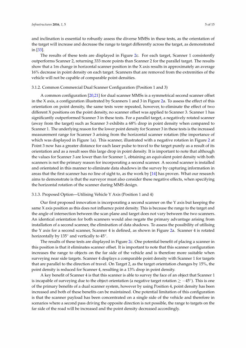
and inclination is essential to robustly assess the diverse MMSs in these tests, as the orientation ofthe target will increase and decrease the range to target differently across the target, as demonstratedin [33].

The results of these tests are displayed in Figure 2c. For each target, Scanner 1 consistentlyoutperforms Scanner 2, returning 333 more points than Scanner 2 for the parallel target. The resultsshow that a 1m change in horizontal scanner position in the X axis results in approximately an average16% decrease in point density on each target. Scanners that are removed from the extremities of thevehicle will not be capable of comparable point densities.

3.1.2. Common Commercial Dual Scanner Configuration (Position 1 and 3)

A common configuration [20,21] for dual scanner MMSs is a symmetrical second scanner offsetin the X axis, a configuration illustrated by Scanners 1 and 3 in Figure 2a. To assess the effect of thisorientation on point density, the same tests were repeated, however, to eliminate the effect of twodifferent X positions on the point density, no scanner offset was applied to Scanner 3. Scanner 1 hassignificantly outperformed Scanner 3 in these tests. For a parallel target, a negatively rotated scanner(away from the target) such as Scanner 3 exhibits a 68% drop in point density when compared toScanner 1. The underlying reason for the lower point density for Scanner 3 in these tests is the increasedmeasurement range for Scanner 3 arising from the horizontal scanner rotation (the importance ofwhich was displayed in Figure 1a). This scanner, illustrated with a negative rotation in Figure 2 atPoint 3 now has a greater distance for each laser pulse to travel to the target purely as a result of itsorientation and as a result sees this large drop in point density. It is important to note that althoughthe values for Scanner 3 are lower than for Scanner 1, obtaining an equivalent point density with bothscanners is not the primary reason for incorporating a second scanner. A second scanner is installedand orientated in this manner to eliminate data shadows in the survey by capturing information inareas that the first scanner has no line of sight to, as the work by [14] has proven. What our researchaims to demonstrate is that the surveyor must also consider these negative effects, when specifyingthe horizontal rotation of the scanner during MMS design.

3.1.3. Proposed Option—Utilising Vehicle Y Axis (Position 1 and 4)

Our first proposed innovation is incorporating a second scanner on the Y axis but keeping thesame X axis position as this does not influence point density. This is because the range to the target andthe angle of intersection between the scan plane and target does not vary between the two scanners.An identical orientation for both scanners would also negate the primary advantage arising frominstallation of a second scanner, the elimination of data shadows. To assess the possibility of utilisingthe Y axis for a second scanner, Scanner 4 is defined, as shown in Figure 2a. Scanner 4 is rotatedhorizontally by 135◦ and vertically to 45◦.

The results of these tests are displayed in Figure 2c. One potential benefit of placing a scanner inthis position is that it eliminates scanner offset. It is important to note that this scanner configurationincreases the range to objects on the far side of the vehicle and is therefore more suitable whensurveying near side targets. Scanner 4 displays a comparable point density with Scanner 1 for targetsthat are parallel to the direction of travel. On Target 2, as the target orientation changes by 15%, thepoint density is reduced for Scanner 4, resulting in a 13% drop in point density.

A key benefit of Scanner 4 is that this scanner is able to survey the face of an object that Scanner 1is incapable of surveying due to the object orientation (a negative target rotation ≥ −45◦). This is oneof the primary benefits of a dual scanner system, however by using Position 4, point density has beenincreased and both of these benefits can be maintained. One potential limitation of this configurationis that the scanner payload has been concentrated on a single side of the vehicle and therefore inscenarios where a second pass driving the opposite direction is not possible, the range to targets on thefar side of the road will be increased and the point density decreased accordingly.

Infrastructures 2016, 1, 5 6 of 15

3.2. Enabling Use of Lower Specification Scanner through Field of View Manipulation

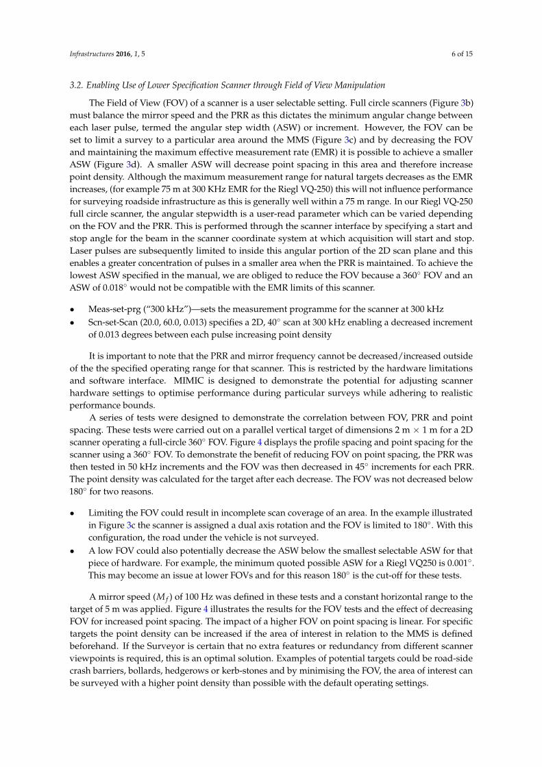
The Field of View (FOV) of a scanner is a user selectable setting. Full circle scanners (Figure 3b)must balance the mirror speed and the PRR as this dictates the minimum angular change betweeneach laser pulse, termed the angular step width (ASW) or increment. However, the FOV can beset to limit a survey to a particular area around the MMS (Figure 3c) and by decreasing the FOVand maintaining the maximum effective measurement rate (EMR) it is possible to achieve a smallerASW (Figure 3d). A smaller ASW will decrease point spacing in this area and therefore increasepoint density. Although the maximum measurement range for natural targets decreases as the EMRincreases, (for example 75 m at 300 KHz EMR for the Riegl VQ-250) this will not influence performancefor surveying roadside infrastructure as this is generally well within a 75 m range. In our Riegl VQ-250full circle scanner, the angular stepwidth is a user-read parameter which can be varied dependingon the FOV and the PRR. This is performed through the scanner interface by specifying a start andstop angle for the beam in the scanner coordinate system at which acquisition will start and stop.Laser pulses are subsequently limited to inside this angular portion of the 2D scan plane and thisenables a greater concentration of pulses in a smaller area when the PRR is maintained. To achieve thelowest ASW specified in the manual, we are obliged to reduce the FOV because a 360◦ FOV and anASW of 0.018◦ would not be compatible with the EMR limits of this scanner.

• Meas-set-prg (“300 kHz”)—sets the measurement programme for the scanner at 300 kHz• Scn-set-Scan (20.0, 60.0, 0.013) specifies a 2D, 40◦ scan at 300 kHz enabling a decreased increment

of 0.013 degrees between each pulse increasing point density

It is important to note that the PRR and mirror frequency cannot be decreased/increased outsideof the the specified operating range for that scanner. This is restricted by the hardware limitationsand software interface. MIMIC is designed to demonstrate the potential for adjusting scannerhardware settings to optimise performance during particular surveys while adhering to realisticperformance bounds.

A series of tests were designed to demonstrate the correlation between FOV, PRR and pointspacing. These tests were carried out on a parallel vertical target of dimensions 2 m × 1 m for a 2Dscanner operating a full-circle 360◦ FOV. Figure 4 displays the profile spacing and point spacing for thescanner using a 360◦ FOV. To demonstrate the benefit of reducing FOV on point spacing, the PRR wasthen tested in 50 kHz increments and the FOV was then decreased in 45◦ increments for each PRR.The point density was calculated for the target after each decrease. The FOV was not decreased below180◦ for two reasons.

• Limiting the FOV could result in incomplete scan coverage of an area. In the example illustratedin Figure 3c the scanner is assigned a dual axis rotation and the FOV is limited to 180◦. With thisconfiguration, the road under the vehicle is not surveyed.

• A low FOV could also potentially decrease the ASW below the smallest selectable ASW for thatpiece of hardware. For example, the minimum quoted possible ASW for a Riegl VQ250 is 0.001◦.This may become an issue at lower FOVs and for this reason 180◦ is the cut-off for these tests.

A mirror speed (M f ) of 100 Hz was defined in these tests and a constant horizontal range to thetarget of 5 m was applied. Figure 4 illustrates the results for the FOV tests and the effect of decreasingFOV for increased point spacing. The impact of a higher FOV on point spacing is linear. For specifictargets the point density can be increased if the area of interest in relation to the MMS is definedbeforehand. If the Surveyor is certain that no extra features or redundancy from different scannerviewpoints is required, this is an optimal solution. Examples of potential targets could be road-sidecrash barriers, bollards, hedgerows or kerb-stones and by minimising the FOV, the area of interest canbe surveyed with a higher point density than possible with the default operating settings.

Infrastructures 2016, 1, 5 7 of 15

(a) (b) (c)

(d)

Figure 3. Changing scanner Field of View (FOV) to improve point spacing (a) point cloud characteristicsfor a mobile mapping system survey using a 2D scanner (b) a full-circle FOV will distribute the maxnumber of pulses per mirror rotation around the full 360◦ (c) decreasing FOV enables a MMS to focuslaser pulses on one side of the vehicle (d) limiting the FOV then allows the max number of pulses permirror rotation to be distributed throughout this reduced FOV, decreasing point spacing.

Figure 4. The effect of changing scanner settings such as Pulse Repetition Rate (PRR), mirror frequencyand decreasing the scanner FOV on the coverage of the environment.

Infrastructures 2016, 1, 5 8 of 15

4. Test Systems

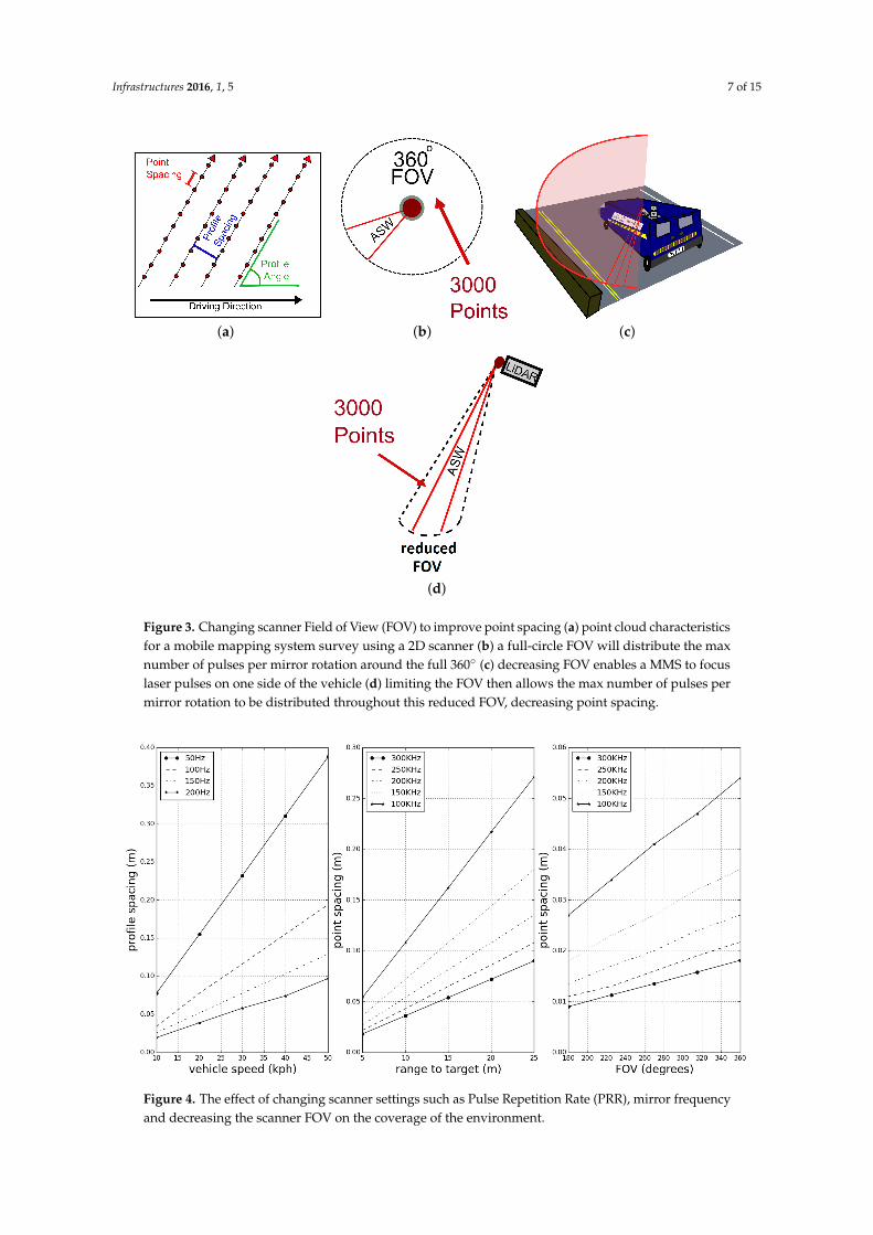
MIMIC enables benchmarking of multiple scanner configurations in terms of their point density.Three MMSs were assessed in these tests, as illustrated in Figure 5. The hardware and configuration ofthese three theoretical MMS are described in this section. One system employs MIMIC to improveperformance, and the second uses a scanner with a high PRR and the second with a high mirror speed.Scanner elevations were standardised for each system at the height of the scanner on the XP1, whichis 3.1 m. This ensured that the results are dependent on the hardware configuration only and notinfluenced by the dimensions of the platform.

(a) (b) (c)

Figure 5. Mobile Mapping Systems (MMS) in benchmarking tests (a) MIMIC+ Scanner Locations (b)PRR+ Scanning Locations (c) Mirror+ locations.

4.1. System 1—MIMIC+

The XP1 designed at the NCG is a single scanner system employing a single VQ-250.Incorporating another high specification scanner can be very costly and increases data throughput onthe MMS and therefore MIMIC was used to identify optimum parameters for incorporating a lowerspecification scanner and maintaining a suitable point density. This system, entitled ’MIMIC+’,incorporates a generic, limited FOV, low PRR laser profiler operating a rotating mirror. Table 1 lists therelevant parameters of the two scanners on the MIMIC+. The PRR of the second scanner was only9% that of the Riegl VQ250. This shortcoming was partially offset by the lower FOV of Scanner 2which decreases the ASW. The two scanners were orientated and positioned in accordance with therecommended configuration identified in [34]. The 60◦ vertical rotation identified in tests [34] wasapplied to both scanners to maximise point density. Horizontal scanner rotations of 45◦ and 135◦ wereapplied respectively.

Table 1. XP1+ Scanner Parameters.

System Scanner Hrot VRot M f PRR FOV ASW

MIMIC+ Geom1 45 60 100 Hz 300 kHz 360◦ 0.12◦

FOV1 135 60 75 Hz 27.075 kHz 180◦ 0.99◦

PRR+ PRR1 45 45 100 Hz 300 kHz 360◦ 0.12◦

PRR2 45 60 100 Hz 300 kHz 360◦ 0.12◦

Mirror+ Mirror1 45 45 200 Hz 200 kHz 360o 0.36◦

Mirror2 45 60 200 Hz 200 kHz 360◦ 0.36◦

4.2. System 2—PRR+

The PRR+ incorporates a second VQ-250 scanner but has retained the XP1’s 45◦/45◦ horizontaland vertical rotations scanner orientation, therefore not using the improved orientation calculated

Infrastructures 2016, 1, 5 9 of 15

using MIMIC. This system is designed to replicate those MMSs that prioritise pulse repetition rate.The second scanner is negatively rotated to −45◦/45◦ as detailed in Table 1. The second scanner wasoffset by 1 m in the X axis, this standard offset is assigned to enable a comparison between the XP2and the Mirror+.

4.3. System 3—Mirror+

The third system was designed to simulate a MMS that prioritises mirror frequency over PRR.These MMSs are capable of a higher mirror frequency PRR systems resulting in more scan lines but thelower PRR results in a reduced point spacing.

5. Benchmarking MMS Performance

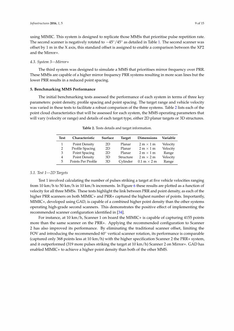
The initial benchmarking tests assessed the performance of each system in terms of three keyparameters: point density, profile spacing and point spacing. The target range and vehicle velocitywas varied in these tests to facilitate a robust comparison of the three systems. Table 2 lists each of thepoint cloud characteristics that will be assessed for each system, the MMS operating parameters thatwill vary (velocity or range) and details of each target type, either 2D planar targets or 3D structures.

Table 2. Tests details and target information.

Test Characteristic Surface Target Dimensions Variable

1 Point Density 2D Planar 2 m × 1 m Velocity2 Profile Spacing 2D Planar 2 m × 1 m Velocity3 Point Spacing 2D Planar 2 m × 1 m Range4 Point Density 3D Structure 2 m × 2 m Velocity5 Points Per Profile 3D Cylinder 0.1 m × 2 m Range

5.1. Test 1—2D Targets

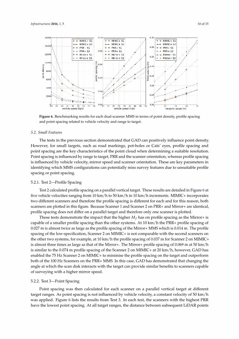
Test 1 involved calculating the number of pulses striking a target at five vehicle velocities rangingfrom 10 km/h to 50 km/h in 10 km/h increments. In Figure 6 these results are plotted as a function ofvelocity for all three MMSs. These tests highlight the link between PRR and point density, as each of thehigher PRR scanners on both MIMIC+ and PRR+ captured the highest number of points. Importantly,MIMIC+, developed using GAD, is capable of a combined higher point density than the other systemsoperating high-grade second scanners. This demonstrates the positive effect of implementing therecommended scanner configuration identified in [34].

For instance, at 10 km/h, Scanner 1 on board the MIMIC+ is capable of capturing 4155 pointsmore than the same scanner on the PRR+. Applying the recommended configuration to Scanner2 has also improved its performance. By eliminating the traditional scanner offset, limiting theFOV and introducing the recommended 60◦ vertical scanner rotation, its performance is comparable(captured only 368 points less at 10 km/h) with the higher specification Scanner 2 the PRR+ system,and it outperformed (319 more pulses striking the target at 10 km/h) Scanner 2 on Mirror+. GAD hasenabled MIMIC+ to achieve a higher point density than both of the other MMS.

Infrastructures 2016, 1, 5 10 of 15

Figure 6. Benchmarking results for each dual-scanner MMS in terms of point density, profile spacingand point spacing related to vehicle velocity and range to target.

5.2. Small Features

The tests in the previous section demonstrated that GAD can positively influence point density.However, for small targets, such as road markings, pot-holes or Cats’ eyes, profile spacing andpoint spacing are the key characteristics of the point cloud when determining a suitable resolution.Point spacing is influenced by range to target, PRR and the scanner orientation, whereas profile spacingis influenced by vehicle velocity, mirror speed and scanner orientation. These are key parameters inidentifying which MMS configurations can potentially miss survey features due to unsuitable profilespacing or point spacing.

5.2.1. Test 2—Profile Spacing

Test 2 calculated profile spacing on a parallel vertical target. These results are detailed in Figure 6 atfive vehicle velocities ranging from 10 km/h to 50 km/h in 10 km/h increments. MIMIC+ incorporatestwo different scanners and therefore the profile spacing is different for each and for this reason, bothscanners are plotted in this figure. Because Scanner 1 and Scanner 2 on PRR+ and Mirror+ are identical,profile spacing does not differ on a parallel target and therefore only one scanner is plotted.

These tests demonstrate the impact that the higher M f has on profile spacing as the Mirror+ iscapable of a smaller profile spacing than the other systems. At 10 km/h the PRR+ profile spacing of0.027 m is almost twice as large as the profile spacing of the Mirror+ MMS which is 0.014 m. The profilespacing of the low-specification, Scanner 2 on MIMIC+ is not comparable with the second scanners onthe other two systems, for example, at 10 km/h the profile spacing of 0.037 m for Scanner 2 on MIMIC+is almost three times as large as that of the Mirror+. The Mirror+ profile spacing of 0.069 m at 50 km/his similar to the 0.074 m profile spacing of the Scanner 2 on MIMIC+ at 20 km/h, however, GAD hasenabled the 75 Hz Scanner 2 on MIMIC+ to minimise the profile spacing on the target and outperformboth of the 100 Hz Scanners on the PRR+ MMS. In this case, GAD has demonstrated that changing theangle at which the scan disk interacts with the target can provide similar benefits to scanners capableof surveying with a higher mirror speed.

5.2.2. Test 3—Point Spacing

Point spacing was then calculated for each scanner on a parallel vertical target at differenttarget ranges. As point spacing is not influenced by vehicle velocity, a constant velocity of 50 km/hwas applied. Figure 6 lists the results from Test 3. In each test, the scanners with the highest PRRhave the lowest point spacing. At all target ranges, the distance between subsequent LiDAR points

Infrastructures 2016, 1, 5 11 of 15

captured by these scanners is over twice as low (43%) as the point spacing of the scanners on theMirror+ MMS. Scanner 2 on MIMIC+ exhibits a higher point spacing in these tests because of itslow PRR. At a range of 25 m, this scanner is exhibiting a point spacing that is over four times (419%)larger than the point spacing of Scanner 2 on PRR+. These results reinforce the significance in selectingthe correct scanner configuration for increasing point density. Because of the application of GADon MIMIC+, Scanner 2 produces comparable point density with Mirror+ and PRR+ scanners in theearlier tests on larger targets. However, these results demonstrate that this scanner is not suitable forsurveying narrow targets at long ranges. For instance, for a target such as a circular road sign of radius0.5 m at a 10 m horizontal range, a point spacing of 0.25 m would return an insufficient number ofpoints to distinguish that object in the point cloud. For this target, it would result in two and possiblyonly one pulse striking the target per mirror rotation. In this scenario, Mirror+ has outperformedMIMIC+ with approximately five to six points on each scan profile whereas the PRR+ MMS performedbest with over ten pulses striking the target per mirror rotation.

5.3. Angled Targets

The preceding tests dealt with parallel, planar targets. However, because the majority of roadsideinfrastructure are angled targets or have multiple faces, in this section, benchmarking tests areconducted to examine the performance of each MMS configuration for multi-faced targets, calculatingpoint density on the angled surfaces of two multi-faced structures. The first structure was representedby three large vertical planes and the second structure, a cylinder, was represented by three narrowvertical planes.

5.3.1. Test 4—Structures

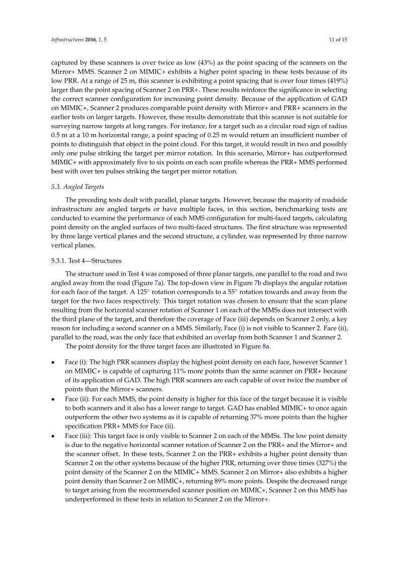
The structure used in Test 4 was composed of three planar targets, one parallel to the road and twoangled away from the road (Figure 7a). The top-down view in Figure 7b displays the angular rotationfor each face of the target. A 125◦ rotation corresponds to a 55◦ rotation towards and away from thetarget for the two faces respectively. This target rotation was chosen to ensure that the scan planeresulting from the horizontal scanner rotation of Scanner 1 on each of the MMSs does not intersect withthe third plane of the target, and therefore the coverage of Face (iii) depends on Scanner 2 only, a keyreason for including a second scanner on a MMS. Similarly, Face (i) is not visible to Scanner 2. Face (ii),parallel to the road, was the only face that exhibited an overlap from both Scanner 1 and Scanner 2.

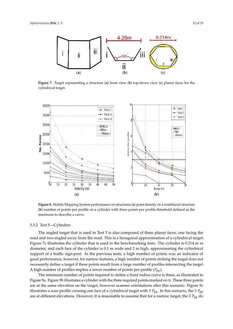
The point density for the three target faces are illustrated in Figure 8a.

• Face (i): The high PRR scanners display the highest point density on each face, however Scanner 1on MIMIC+ is capable of capturing 11% more points than the same scanner on PRR+ becauseof its application of GAD. The high PRR scanners are each capable of over twice the number ofpoints than the Mirror+ scanners.

• Face (ii): For each MMS, the point density is higher for this face of the target because it is visibleto both scanners and it also has a lower range to target. GAD has enabled MIMIC+ to once againoutperform the other two systems as it is capable of returning 37% more points than the higherspecification PRR+ MMS for Face (ii).

• Face (iii): This target face is only visible to Scanner 2 on each of the MMSs. The low point densityis due to the negative horizontal scanner rotation of Scanner 2 on the PRR+ and the Mirror+ andthe scanner offset. In these tests, Scanner 2 on the PRR+ exhibits a higher point density thanScanner 2 on the other systems because of the higher PRR, returning over three times (327%) thepoint density of the Scanner 2 on the MIMIC+ MMS. Scanner 2 on Mirror+ also exhibits a higherpoint density than Scanner 2 on MIMIC+, returning 89% more points. Despite the decreased rangeto target arising from the recommended scanner position on MIMIC+, Scanner 2 on this MMS hasunderperformed in these tests in relation to Scanner 2 on the Mirror+.

Infrastructures 2016, 1, 5 12 of 15

(a) (b) (c)

Figure 7. Target representing a structure (a) front view (b) top-down view (c) planar faces for thecylindrical target.

(a) (b)

Figure 8. Mobile Mapping System performance on structures (a) point density on a multifaced structure(b) number of points per profile on a cylinder with three points per profile threshold defined as theminimum to describe a curve.

5.3.2. Test 5—Cylinders

The angled target that is used in Test 5 is also composed of three planar faces, one facing theroad and two angled away from the road. This is a hexagonal approximation of a cylindrical target.Figure 7c illustrates the cylinder that is used in the benchmarking tests. The cylinder is 0.214 m indiameter, and each face of the cylinder is 0.1 m wide and 2 m high, approximating the cylindricalsupport of a traffic sign-post. In the previous tests, a high number of points was an indicator ofgood performance, however, for narrow features, a high number of points striking the target does notnecessarily define a target if these points result from a large number of profiles intersecting the target.A high number of profiles implies a lower number of points per profile (Ppp).

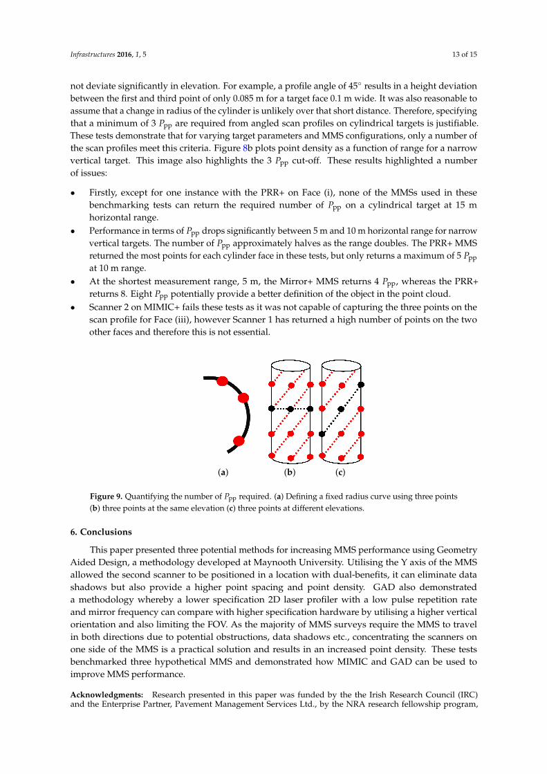
The minimum number of points required to define a fixed radius curve is three, as illustrated inFigure 9a. Figure 9b illustrates a cylinder with the three required points marked on it. These three pointsare at the same elevation on the target, however scanner orientations alter this scenario. Figure 9cillustrates a scan profile crossing one face of a cylindrical target with 3 Ppp. In this scenario, the 3 Ppp

are at different elevations. However, it is reasonable to assume that for a narrow target, the 3 Ppp do

Infrastructures 2016, 1, 5 13 of 15

not deviate significantly in elevation. For example, a profile angle of 45◦ results in a height deviationbetween the first and third point of only 0.085 m for a target face 0.1 m wide. It was also reasonable toassume that a change in radius of the cylinder is unlikely over that short distance. Therefore, specifyingthat a minimum of 3 Ppp are required from angled scan profiles on cylindrical targets is justifiable.These tests demonstrate that for varying target parameters and MMS configurations, only a number ofthe scan profiles meet this criteria. Figure 8b plots point density as a function of range for a narrowvertical target. This image also highlights the 3 Ppp cut-off. These results highlighted a numberof issues:

• Firstly, except for one instance with the PRR+ on Face (i), none of the MMSs used in thesebenchmarking tests can return the required number of Ppp on a cylindrical target at 15 mhorizontal range.

• Performance in terms of Ppp drops significantly between 5 m and 10 m horizontal range for narrowvertical targets. The number of Ppp approximately halves as the range doubles. The PRR+ MMSreturned the most points for each cylinder face in these tests, but only returns a maximum of 5 Ppp

at 10 m range.• At the shortest measurement range, 5 m, the Mirror+ MMS returns 4 Ppp, whereas the PRR+

returns 8. Eight Ppp potentially provide a better definition of the object in the point cloud.• Scanner 2 on MIMIC+ fails these tests as it was not capable of capturing the three points on the

scan profile for Face (iii), however Scanner 1 has returned a high number of points on the twoother faces and therefore this is not essential.

(a) (b) (c)

Figure 9. Quantifying the number of Ppp required. (a) Defining a fixed radius curve using three points(b) three points at the same elevation (c) three points at different elevations.

6. Conclusions

This paper presented three potential methods for increasing MMS performance using GeometryAided Design, a methodology developed at Maynooth University. Utilising the Y axis of the MMSallowed the second scanner to be positioned in a location with dual-benefits, it can eliminate datashadows but also provide a higher point spacing and point density. GAD also demonstrateda methodology whereby a lower specification 2D laser profiler with a low pulse repetition rateand mirror frequency can compare with higher specification hardware by utilising a higher verticalorientation and also limiting the FOV. As the majority of MMS surveys require the MMS to travelin both directions due to potential obstructions, data shadows etc., concentrating the scanners onone side of the MMS is a practical solution and results in an increased point density. These testsbenchmarked three hypothetical MMS and demonstrated how MIMIC and GAD can be used toimprove MMS performance.

Acknowledgments: Research presented in this paper was funded by the the Irish Research Council (IRC)and the Enterprise Partner, Pavement Management Services Ltd., by the NRA research fellowship program,

Infrastructures 2016, 1, 5 14 of 15

ERA-NET SR01 projects and by a Strategic Research Cluster grant (07/SRC/I1168) from Science FoundationIreland under the National Development Plan.

Author Contributions: MIMIC was developed by Conor Cahalane. Paul Lewis, Eimear McNerney andConor P. McElhinney collaborated with Cahalane in identifying and designing each test. Tim McCarthy providedtechnical advice at all stages. All authors contributed equally in preparing this manuscript.

Conflicts of Interest: The authors declare no conflict of interest.

References

1. Puente, I.; González-Jorge, H.; Martínez-Sánchez, J.; Arias, P. Review of mobile mapping andsurveying technologies. Measurement 2013, 46, 2127–2145.

2. Graham, L. Mobile mapping systems overview. Photogramm. Eng. Remote Sens. 2010, 76, 222–228.3. McElhinney, C.; Kumar, P.; Cahalane, C.; McCarthy, T. Initial results from European Road Safety Inspection

(EURSI) mobile mapping project. In Proceedings of the ISPRS Commission V Technical Symposium,Newcastle, UK, 21–24 June 2010.

4. Becker, S.; Haala, N. Grammar supported facade reconstruction from mobile LiDAR mapping.In Proceedings of the ISPRS CMRT09, Paris, France, 3–4 September 2009; pp. 229–234.

5. Hammoudi, K.; Dornaika, F.; Paparoditis, N. Extracting building footprints from 3D point cloudsusing terrestrial laser scanning at street level. In Proceedings of the ISPRS CMRT09, Paris, France,3–4 September 2009; pp. 65–70.

6. Kumar, P.; McCarthy, T.; McElhinney, C. Automated road extraction from terrestrial based mobilelaser scanning system using the GVF snake model. In Proceedings of the European Laser MappingForum—’ELMF 2010’, The Hague, The Netherlands, 30 November–1 December 2010.

7. Kumar, P.; McElhinney, C.; McCarthy, T. Utilizing terrestrial mobile laser scanning data attributes for roadedge extraction with the GVF snake model. In Proceedings of the 7th International Symposium on MobileMapping Technology (MMT’11), Cracow, Poland, 13–16 June 2011.

8. Pu, S.; Vosselman, G. Extracting windows from terrestrial laser scanning. In Proceedings of the ISPRSWorkshop on Laser Scanning 2007 and SilviLaser 2007, Espoo, Finland, 12–14 September 2007; Volume 36,pp. 320–325.

9. Pu, S.; Rutzinger, M.; Vosselman, G.; Elberink, S.O. Recognizing basic structures from mobile laser scanningdata for road inventory studies. ISPRS J. Photogramm. Remote Sens. 2011, 66, S28–S39.

10. Brenner, C. Global localization of vehicles using local pole patterns. In Pattern Recognition; Denzler, J.,Notni, G., Süße, H., Eds.; Lecture Notes in Computer Science; Springer: Berlin/Heidelberg, Germany, 2009;Volume 5748, pp. 61–70.

11. Kukko, A.; Jaakkola, A.; Lehtomaki, M.; Kaartinen, H.; Chen, Y. Mobile mapping system and computingmethods for modelling of road environment. In Proceedings of the 2009 Joint Urban Remote Sensing Event,Shanghai, China, 20–22 May 2009.

12. Lehtomäki, M.; Jaakkola, A.; Hyyppä, J.; Kukko, A.; Kaartinen, H. Detection of vertical pole-like objects ina road environment using vehicle-based laser scanning data. Remote Sens. 2010, 2, 641–664.

13. Kaartinen, H.; Hyyppä, J.; Gülch, E.; Vosselman, G.; Hyyppä, H.; Matikainen, L.; Hofmann, A.D.;Mäder, U.; Persson, A. Accuracy of 3D City Models: EuroSDR comparison. In Proceedings of theInternational Archives of Photogrammetry, Remote Sensing and Spatial Information Sciences, Enschede,The Netherlands, 12–14 September 2005; pp. 227–232.

14. Yoo, H.; Goulette, F.; Senpauroca, J.; Lepere, G. Simulation based comparative analysis for the design oflaser terresttrial mobile mapping. In Proceedings of the 6th International Symposium on Mobile MappingTechnology, Sao Paulo, Brazil, 21–24 July 2009; pp. 839–854.

15. Bolzon, G.; Caroti, G.; Piemonte, A. Accuracy check of road’s cross slope evaluation using MMSvehicle. In Proceedings of the 5th International Symposium on Mobil Mapping Technology, Padua,Italy, 28–31 May 2007; pp. 127–132.

16. Florida Department of Transport. Terrestrial Mobile LiDAR Surveying and Mapping Guidelines;Florida Department of Transport: Tallahassee, FL, USA, 2012.

17. Yen, K.S.; Ravani, B.; Lasky, T.A. LiDAR for Data Efficiency; University of California: Oakland, CA,USA, 2011.

Infrastructures 2016, 1, 5 15 of 15

18. Olsen, M.J.; Roe, G.V.; Glennie, C.; Persi, F.; Reedy, M.; Hurwitz, D.; Williams, K.; Tuss, H.; Squellati, A.;Knodler, M. NCHRP 15–44 Guidelines for the Use of Mobile LiDAR in Transportation Applications; NCHRP:Washington, DC, USA, 2013.

19. Trimble. Trimble MX8 Mobile Mapping System; Trimble: Sunnyvale, CA, USA, 2010.20. Optech. Optech Lynx M1 and V200 System Specifications; Optech: Vaughan, ON, Canada, 2012.21. RIEGL. Dual Scanner Data Sheet Riegl VMX-450; RIEGL: Horn, Austria, 2016.22. Laser Mapping. StreetMapper Brochure; Technical Report; 3D Laser Mapping: Nottingham, UK, 2012.23. Kukko, A.; Andrei, C.; Salminen, V.; Kaartinen, H.; Chen, Y.; Rönnholm, P.; Hyyppä, H.; Hyyppä, J.;

Chen, R.; Haggrén, H.; et al. Road environment mapping system of the finnish geodetic institute-FGIroamer. In Proceedings of the ISPRS Workshop on Laser Scanning 2007 and SilviLaser 2007, Espoo, Finland,12–14 September 2007; pp. 241–247.

24. Hesse, C.; Kutterer, H. A mobile mapping system using kinematic terrestrial laser scanning (KTLS) forimage acquisition. In Proceedings of the 8th Conference on Optical 3-D Measurement Techniques, Zurich,Switzerland, 9–12 July 2007; pp. 134–141.

25. Lohani, B.; Mishra, R. Generating LiDAR data in laboratory: LiDAR simulator. In Proceedings of the ISPRSWorkshop on Laser Scanning 2007 and SilviLaser 2007, Espoo, Finland, 12–14 September 2007; Volume 52,pp. 12–14.

26. Kukko, A.; Hyyppä, J. Small-footprint laser scanning simulator for system validation, error assessmentand algorithm development. Photogramm. Eng. Remote Sens. 2009, 75, 1177–1189.

27. Kaartinen, H.; Hyyppä, J.; Kukko, A.; Jaakkola, A.; Hyyppä, H. Benchmarking the performance of mobilelaser scanning systems using a permanent test field. Sensors 2012, 12, 12814–12835.

28. Cahalane, C.; McCarthy, T.; McElhinney, C. MIMIC: Mobile mapping point density calculator.In Proceedings of the 3rd International Conference on Computing for Geospatial Research and Applications,Reston, VA, USA, 1–3 July 2012.

29. Cahalane, C.; McCarthy, T.; McElhinney, C. Mobile mapping system performance: An initial investigationinto the effect of vehicle speed on laser scan lines. In Proceedings of the Remote Sensing & PhotogrammetySociety Annual Conference—‘From the Sea-Bed to the Cloudtops’, Cork, Ireland, 1–3 September 2010.

30. Cahalane, C.; McElhinney, C.; McCarthy, T. Mobile mapping system performance: An analysis of the effectof laser scanner configuration and vehicle velocity on scan profiles. In Proceedings of the European laserMapping Forum—‘ELMF 2010’, The Hague, The Netherlands, 30–31 November 2010.

31. Cahalane, C.; McElhinney, C.; McCarthy, T. Calculating the effect of dual-axis scanner rotations and surfaceorientation on scan profiles. In Proceedings of the 7th International Symposium on Mobile MappingTechnology (MMT’11), Cracow, Poland, 13–16 June 2011.

32. Cahalane, C.; McElhinney, C.; Lewis, P.; McCarthy, T. Calculation of target-specific point distribution for2D mobile laser scanners. Sensors 2014, 14, 9471–9488.

33. Cahalane, C.; McElhinney, C.; Lewis, P.; McCarthy, T. MIMIC: An innovative methodology for determiningmobile laser scanning system point density. Remote Sens. 2014, 6, 7857–7877.

34. Cahalane, C.; Lewis, P.; McElhinney, C.; McCarthy, T. Optimising mobile mapping system laserscanner orientation. ISPRS Int. J. Geo-Inf. 2015, 4, 302–319.

35. Shepard, D. A two-dimensional interpolation function for irregularly-spaced data. In Proceedings of the23rd National Conference ACM, Las Vegas, NV, USA, 27–29 August 1968; pp. 517–524.

c© 2016 by the authors; licensee MDPI, Basel, Switzerland. This article is an open accessarticle distributed under the terms and conditions of the Creative Commons Attribution(CC-BY) license (http://creativecommons.org/licenses/by/4.0/).