Improving Optical Flow using Residual and Sobel Edge Images Tobi Vaudrey 1 , Andreas Wedel 2 , Chia-Yen Chen 3 , and Reinhard Klette 1 1 The .enpeda.. Project, The University of Auckland, Auckland, New Zealand 2 Daimler Research, Daimler AG, Stuttgart, Germany 3 National University of Kaohsiung, Taiwan Abstract. Optical flow is a highly researched area in low-level computer vision. It is a complex problem which tries to solve a 2D search in contin- uous space, while the input data is 2D discrete data. Furthermore, the latest representations of optical flow use Hue-Saturation-Value (HSV) colour circles, to effectively convey direction and magnitude of vectors. The major assumption in most optical flow applications is the inten- sity consistency assumption, introduced by Horn and Schunck. This con- straint is often violated in practice. This paper proposes and generalises one such approach; using residual images (high-frequencies) of images, to remove the illumination differences between corresponding images. 1 Introduction Dense optical flow was first presented by Horn and Schunck [8]. Their approach exploited the intensity consistency assumption (ICA), coupled with a smoothness constraint. This was solved in a variational approach. Many more approaches have been proposed since this, most using this basic ICA and smoothness con- straint. In recent years, the use of pyramids, warping and robust minimisation equations have improved results dramatically [3]. This has further been improved and computational enhancement in [21]. Fig. 1. Example frames from EISATS scene. Frame 1 (left) and 2 (middle) are shown with ground truth flow (right) also showing the color key (HSV circle for direction, saturation for vector length, max saturation at flow length 10).
Transcript
Improving Optical Flow usingResidual and Sobel Edge Images
Tobi Vaudrey1, Andreas Wedel2, Chia-Yen Chen3, and Reinhard Klette1
1 The .enpeda.. Project, The University of Auckland, Auckland, New Zealand2 Daimler Research, Daimler AG, Stuttgart, Germany
3 National University of Kaohsiung, Taiwan
Abstract. Optical flow is a highly researched area in low-level computervision. It is a complex problem which tries to solve a 2D search in contin-uous space, while the input data is 2D discrete data. Furthermore, thelatest representations of optical flow use Hue-Saturation-Value (HSV)colour circles, to effectively convey direction and magnitude of vectors.The major assumption in most optical flow applications is the inten-sity consistency assumption, introduced by Horn and Schunck. This con-straint is often violated in practice. This paper proposes and generalisesone such approach; using residual images (high-frequencies) of images,to remove the illumination differences between corresponding images.
1 Introduction
Dense optical flow was first presented by Horn and Schunck [8]. Their approachexploited the intensity consistency assumption (ICA), coupled with a smoothnessconstraint. This was solved in a variational approach. Many more approacheshave been proposed since this, most using this basic ICA and smoothness con-straint. In recent years, the use of pyramids, warping and robust minimisationequations have improved results dramatically [3]. This has further been improvedand computational enhancement in [21].
Fig. 1. Example frames from EISATS scene. Frame 1 (left) and 2 (middle) are shownwith ground truth flow (right) also showing the color key (HSV circle for direction,saturation for vector length, max saturation at flow length 10).
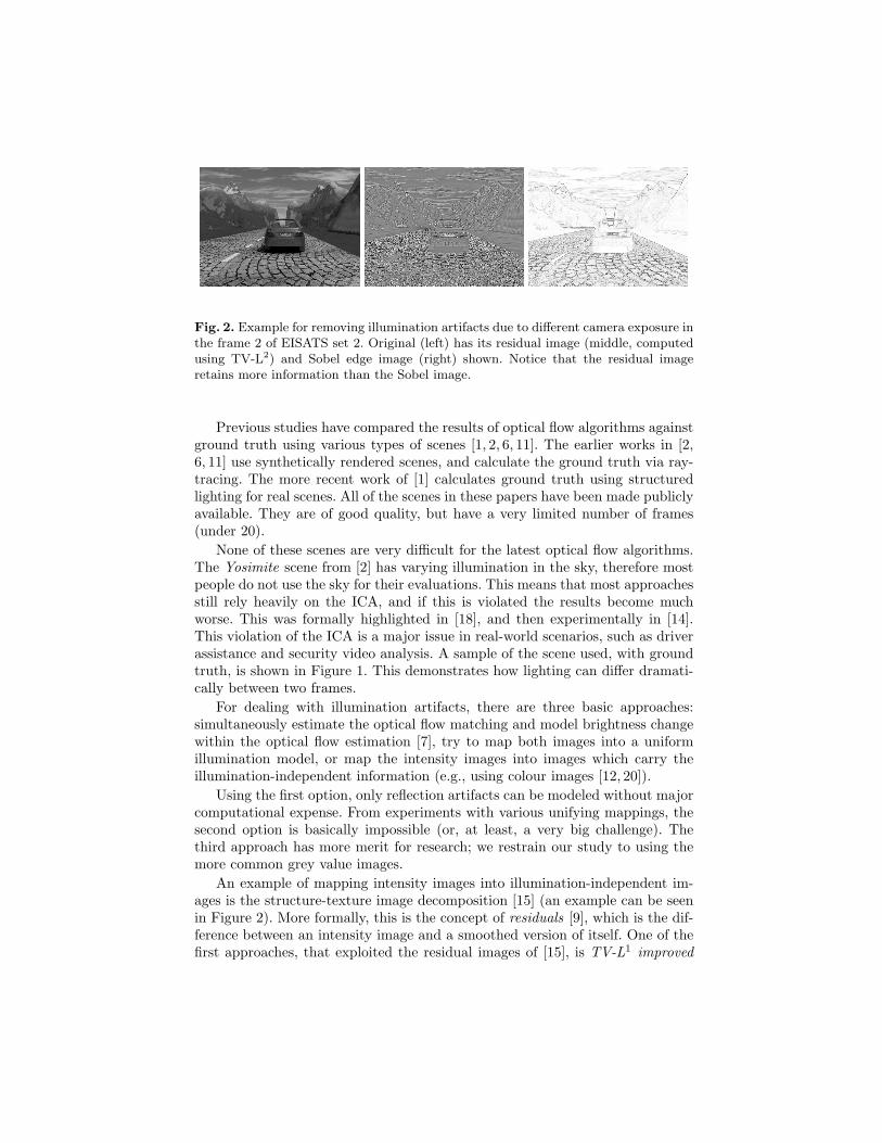
Fig. 2. Example for removing illumination artifacts due to different camera exposure inthe frame 2 of EISATS set 2. Original (left) has its residual image (middle, computedusing TV-L2) and Sobel edge image (right) shown. Notice that the residual imageretains more information than the Sobel image.
Previous studies have compared the results of optical flow algorithms againstground truth using various types of scenes [1, 2, 6, 11]. The earlier works in [2,6, 11] use synthetically rendered scenes, and calculate the ground truth via ray-tracing. The more recent work of [1] calculates ground truth using structuredlighting for real scenes. All of the scenes in these papers have been made publiclyavailable. They are of good quality, but have a very limited number of frames(under 20).
None of these scenes are very difficult for the latest optical flow algorithms.The Yosimite scene from [2] has varying illumination in the sky, therefore mostpeople do not use the sky for their evaluations. This means that most approachesstill rely heavily on the ICA, and if this is violated the results become muchworse. This was formally highlighted in [18], and then experimentally in [14].This violation of the ICA is a major issue in real-world scenarios, such as driverassistance and security video analysis. A sample of the scene used, with groundtruth, is shown in Figure 1. This demonstrates how lighting can differ dramati-cally between two frames.
For dealing with illumination artifacts, there are three basic approaches:simultaneously estimate the optical flow matching and model brightness changewithin the optical flow estimation [7], try to map both images into a uniformillumination model, or map the intensity images into images which carry theillumination-independent information (e.g., using colour images [12, 20]).
Using the first option, only reflection artifacts can be modeled without majorcomputational expense. From experiments with various unifying mappings, thesecond option is basically impossible (or, at least, a very big challenge). Thethird approach has more merit for research; we restrain our study to using themore common grey value images.
An example of mapping intensity images into illumination-independent im-ages is the structure-texture image decomposition [15] (an example can be seenin Figure 2). More formally, this is the concept of residuals [9], which is the dif-ference between an intensity image and a smoothed version of itself. One of thefirst approaches, that exploited the residual images of [15], is TV-L1 improved
optical flow [19], which is an improvement to the original TV-L1 proposed in[21]. A residual is, in fact, an approximation of a high-pass filter, so only highfrequencies remain present.
In this paper we generalise the residual operator by using any smoothingoperator to calculate the low frequencies. Included in this study are three edge-preserving filters (TV-L2 [15], median, bilateral [17]), two general filters (meanand Gaussian), and a gradient preserving filter (trilateral [4]). Furthermore, weuse an edge detector as a reference (Sobel [16]). This paper shows experimentallythat any residual image is better than the original image when illuminationvariance is causing issues.
2 Smoothing Operators and Residuals
Let f be any frame of a given image sequence, defined on a rectangular open setΩ and sampled at regular grid points within Ω.
f can be defined to have an additive decomposition f(x) = s(x) + r(x), forall pixel positions x = (x, y), where s = S(f) denotes the smooth component (ofan image) and r = R(f) = f − S(f) the residual (Figure 2 shows an example ofthe decomposition). We use the straightforward iteration scheme:
s(0) = f, s(n+1) = S(s(n)), r(n+1) = f − s(n+1), for n ≥ 0.
The concept of residual images was already introduced in [9] by using a 3 × 3mean for implementing S. We apply the m×m mean operator and also an m×mmedian operator in this study. Furthermore, we use an m ×m Gaussian filter,with σ for the normal approximation. The other operators for S are definedbelow.
TV-L2 filter: [15] assumed an additive decomposition f = s + r into asmooth component s and a residual component r, where s is assumed to be inL1(Ω) with bounded TV (in brief: s ∈ BV), and r is in L2(Ω). This allows oneto consider the minimization of the following functional:
inf(s,r)∈BV×L2∧f=s+r
(∫Ω
|∇s|+ λ||r||2L2
)(1)
The TV-L2 approach in [15] was approximating this minimum numerically foridentifying the “desired clean image” s and “additive noise” r. See Figure 2.The concept may be generalized as follows: any smoothing operator S generatesa smoothed image s = S(f) and a residuum r = f − S(f). For example, TV-L2
generates the smoothed image s = STV (f) by solving Equ. (1).Sigma filter: This operator [10] is effectively a trimmed mean filter; it uses
an m × m window, but only calculates the mean for all pixels with values in[a − σf , a + σf ], where a is the central pixel value and σf is a threshold. Wechose σf to be the standard deviation of f (to reduce parameters for the filter).
Bilateral filter: This edge-preserving Gaussian filter [17] is used in thespatial domain (using σ2 as spatial σ), also considering changes in the colour
domain (e.g., at object boundaries). In this case, offset vectors a and position-dependent real weights d1(a) define a local convolution, and the weights d1(a)are further scaled by a second weight function d2, defined on the differencesf(x + a)− f(x):
s(x) =1
k(x)
∫Ω
f(x + a) · d1(a) · d2 [f(x + a)− f(x)] da (2)
k(x) =∫Ω
d1(a) · d2 [f(x + a)− f(x)] da
Function k(x) is used for normalization. In this paper, weights d1 and d2 aredefined by Gaussian functions with standard deviations σ1 and σ2, respectively.The smoothed function s equals SBL(f). It therefore only takes into consider-ation values within a Gaussian kernel (σ2 for spatial domain, f for kernel size)within the colour domain (σ1 as colour σ).
Trilateral filter: This gradient-preserving smoothing operator [4] (i.e., ituses the local gradient plane to smooth the image) only requires the specificationof one parameter σ1, which is equivalent to the spatial kernel size. The rest ofthe parameters are self tuning.
It combines two bilateral filters to produce this effect. At first, a bilateralfilter is applied on the derivatives of f (i.e., the gradients):
gf (x) =1
k∇(x)
∫Ω
∇f(x + a) · d1(a) · d2 (||∇f(x + a)−∇f(x)||) da (3)
k∇(x) =∫Ω
d1(a) · d2 (||∇f(x + a)−∇f(x)||) da
Simple forward differences ∇f(x, y) ≈ (f(x+1, y)−f(x, y), f(x, y+1)−f(x, y))are used for the digital image. For the subsequent second bilateral filter, [4]suggested the use of the smoothed gradient gf (x) [instead of ∇f(x)] for es-timating an approximating plane pf (x,a) = f(x) + gf (x) · a Let f4(x,a) =f(x + a)− pf (x,a). Furthermore, a neighbourhood function
n(x,a) =
1 if ||gf (x + a)− gf (x)|| < A0 otherwise (4)
is used for the second weighting. A specifies the adaptive region and is discussedfurther below. Finally,
s(x) = f(x) +1
k4(x)
∫Ω
f4(x,a) · d1(a) · d2(f4(x,a)) · n(x,a) da (5)
k4(x) =∫Ω
d1(a) · d2(f4(x,a)) · n(x,a) da
The smoothed function s equals STL(f). Again, d1 and d2 are assumed tobe Gaussian functions, with standard deviations σ1 and σ2, respectively. Themethod requires specification of parameter σ1 only, which is at first used to be
the radius of circular neighbourhoods at x in f ; let gf (x) be the mean gradientof f in such a neighbourhood. Let
σ2 = 0.15 · ||maxx∈Ω
gf (x)−minx∈Ω
gf (x)|| (6)
(Value 0.15 was recommended in [4]). Finally, also use A = σ2.Numerical Implementation: All filters have been implemented in OpenCV,
where possible the native function was used. For the TV-L2, we use an imple-mentation (with identical parameters) as in [19]. All other filters used are vir-tually parameterless (except a window size) and we use a window size of m = 3(σ1 = 3 for trilateral filter4). For the bilateral filter, we use color standard devi-ation σ1 = Ir/10, where Ir is the range of the intensity values (i.e., σ1 = 0.2 forthe scaled images). The default value of σ = 0.95 is used for the Gaussian filter.All images are scaled to the range −1 < h(x) < 1 using normalisation.
In our analysis, we also use Sobel edge images [16]; this operator providesa normalised gradient function. This is another form of illumination invariantimages.
3 Optical Flow on EISATS Dataset
One of the most influential evaluations of optical flow in recent years is fromMiddlebury Vision Group [1]. This dataset is used to evaluate optical flow inrelatively simple situations. To highlight the effect of using residual images,we used a high ranking (see [13]) optical flow technique called TV-L1 opticalflow [21]. The results for optical flow were analysed on the EISATS dataset [5];see [18] for Set 2 (see below for details). Numerical details of implementation aregiven in [19]. The specific parameters used were:
Smoothness: 35 Duality threshold θ: 0.2 TV step size: 0.25# of pyramid levels: 10 # of iterations / level: 5 # of warps / iteration: 25
The flow field is computed using U(h1, h2) = u. This is to show that aresidual image r provides better data for matching than for the original imagef . We computed the flow using U(r(n)
1 , r(n)2 ) with n = 1, 10, 50, and 100 to show
how each filter behaves. The results are compared to optical flow on the originalimages U(f1, f2), and also for the Sobel-edge images. Figure 4 shows an exampleof this effect, obviously the residual image vastly improves optical flow results.In fact, the original image results are so noisy that they cannot be used.
EISATS Synthetic Dataset: This dataset was made public in [18] for Set2 and is available from [5]. We are only interested in bad illumination conditions.We therefore use the altered data to resemble illumination differences in time, asperformed in [14]; the differences start high between frames, then go to zero at
4 The authours thank Prasun Choudhury (Adobe Systems, Inc.) and Jack Tumblin(EECS, Northwestern University), for their implementation of the trilateral filter.
n TV-L2 Sigma Mean Median Bilateral Trilateral Gaussian Original Sobel
Table 1. Results of TV-L1 optical flow on EISATS sequence. Results are shown fordifferent numbers n of iterations. Statistics are presented for the average (Ave.), zero-mean standard deviation (ZMSD), and the rank based on ZMSD.
frame 50, then increase again. For all t (frame number) we alter the original imagef using a constant brightness, using f(x) = f(x) + c. The constant brightnesschange is defined by: even values of t, c = t− 52, and odd values of t, c = 51− t.An example of the data used can be seen in Figure 1, and the brightness changeover the sequence can be seen in Figure 3.
‐50
0
50
0 10 20 30 40 50 60 70 80 90 100
Brigtness
Frame #
Fig. 3. Graph showing brightness change over sequence for EISATS dataset 2.
Results: To compare the results numerically, we calculated the end-point-error (EPE) as used in [1], which is basically a 2D-root mean squared error. Theresults can be seen in Figure 5. The zoomed out graph highlights that the resultsfor the original image are unusable. The shape of the graph is appropriate aswell, because the difference between intensities of the images gets closer togethernear the middle of the sequence, and further away near the end. The zoomedgraph shows the EPE values between 0.5 and 7.
A major point to highlight is that at different frames in the sequence, thereare different rankings for the filters. If you look, for example, at the n = 100graph at frame 25, the rank is (best to worst): Sobel, trilateral, bilateral, sigma,TV-L2, median, Gaussian, then mean. But if you look at frame 75 (roughly thesame difference in illumination) the rank is (best to worst): mean, Sobel, bilat-eral, trilateral, median, sigma, TV-L2, with Gaussian coming last; a completelydifferent order! From this it should be obvious that a smaller dataset will not
Fig. 4. Sample optical flow results on EISATS scene. Colour is encoded as in Figure 1.Top row (left to right): Using original images, Sobel edge images, and trilateral filter.Middle row (left to right): Gaussian, mean, and sigma filter. Bottom row (left to right):Median, bilateral, and TV-L2 filter.
100
120
140
160
int E
rror
OriginalTV‐L2SigmaMean
0
20
40
60
80
0 10 20 30 40 50 60 70 80 90 100
End Po
i
Frame in Sequence
MedianBilateralTrilateralGaussianSobel
q
4.5
5.5
6.5
int E
rror
0.5
1.5
2.5
3.5
0 10 20 30 40 50 60 70 80 90 100
End Po
i
Frame in Sequenceq
Fig. 5. End-Point-Error results over entire EISATS sequence. Filter iterations r(n) ofn = 100 are shown. The left shows how different the magnitude is for the originalsequence, and the right hand graph is zoomed in between 0.5 and 7.
pick up on these subtleties, so a large dataset (such as a long sequence) is aprerequisite for better understanding of the behaviour of an algorithm.
Since we have such a large dataset (99 results, 100 frames) we calculatedthe average and zero-mean standard deviation (ZMSD) for different iterationnumbers n = 1, 10, 50, and 100. These results are shown in Table 1. Obviously,the original images are far worse than any residual image. From this table youcan see that the order of the rankings shift around depending on the numberof iterations for the residual image n. Another point to note is that the Sobelfilter (which has only 1 iteration) is the best until 50 iterations; this is whenbilateral filtering is the best. Simple mean filtering (which is much faster thanany other filter) comes in at rank 5 after 50 iterations, and gets better around100 iterations. It is notable that the difference between the average and ZMSDhighlights how volatile the results are, the closer together the numbers, the moreconsistent the results.
4 Conclusions and Future Research
We have demonstrated how different residual images effect the results of opticalflow. Any residual image is better than the original optical flow when using theillumination adjusted dataset. It turns out that bilateral filter may be the best,but a Sobel filter or mean residual image will work as well. So far, only simpleresidual images and Sobel images have been tested. Other smoothing algorithmsand illumination invariant models need to be tested, such as those exploitingphase information. Finally, a larger dataset can be used to further verify theillumination artifact reducing effects of residual images.
References
1. Baker, S., Scharstein, D., Lewis, J. P., Roth, S., Black, M., and Szeliski, R.: Adatabase and evaluation methodology for optical flow, in Proc. ICCV, pages 1–8(2007)
2. Barron, J. L., Fleet, D. J., Beauchemin, S. S.: Performance of optical flow tech-niques. In Int. J. of Computer Vision, 12(1): 43–77 (1994)
3. Brox, T., Bruhn, A., Papenberg, N., and Weickert, J.: High accuracy optical flowestimation based on a theory for warping. In Proc. ECCV, pages 25–36 (2004)
4. Choudhury, P., and Tumblin, J.: The trilateral filter for high contrast images andmeshes. In Proc. Eurographics Symp. Rendering, pages 1–11 (2003)
5. .enpeda.. dataset 2 (EISATS): http://www.mi.auckland.ac.nz/EISATS6. Galvin, B., McCane, B., Novins, K., Mason, D., and Mills, S.: Recovering motion
fields: an evaluation of eight optical flow algorithms. In Proc. 9th British MachineVision Conf., pages 195–204 (1998)
7. Haussecker, H. and Fleet, D. J.: Estimating optical flow with physical models ofbrightness variation. IEEE Trans. Pattern Analysis Machine Intelligence, 23:661–673 (2001)
8. Horn, B. K. P., and Schunck, B. G.: Determining optical flow. Artificial Intelligence,17:185–203 (1981)
9. Kuan, D. T., Sawchuk, A. A., Strand, T. C., and Chavel, P.: Adaptive noise smooth-ing filter for images with signal-dependent noise. IEEE Trans. Pattern AnalysisMachine Intelligence, 7:165–177 (1985)
10. Lee, J.-S.: Digital image smoothing and the sigma filter. Computer Vision, Graph-ics, and Image Processing, 24:255–269 (1983)
11. McCane, B., Novins, K., Crannitch, D., and Galvin, B.: On benchmarking opticalflow, In Computer Vision and Image Understanding, 84: 126–143 (2001)
12. Mileva, Y., Bruhn, A. and Weickert, J.: Illumination-robust variational optical flowwith photometric invariants. In Proc. Pattern Recognition - DAGM, pages 152–162(2007)
13. Middlebury Optical Flow Evaluation: http://vision.middlebury.edu/flow/14. Morales, S., Woo, Y. W., Klette, R., and Vaudrey, T.: A study on stereo and motion
data accuracy for a moving platform. In Proc. Int. Conf. on Social Robotics (ICSR),to appear (2009)
15. Rudin, L., Osher, S., and Fatemi, E.: Nonlinear total variation based noise removalalgorithms. Physica D, 60:259–268 (1992)
16. Sobel, I., and Feldman,G.: A 3x3 isotropic gradient operator for image processing,in Pattern Classification and Scene Analysis, pages 271–272 (1973).
17. Tomasi, C., and Manduchi, R.: Bilateral filtering for gray and color images. InProc. IEEE Int. Conf. Computer Vision, pages 839–846 (1998)
18. Vaudrey, T., Rabe, C., Klette, R., and Milburn, J.: Differences betweenstereo and motion behaviour on synthetic and real-world stereo sequences. InProc. IEEE Image and Vision Conf. New Zealand, Digital Object Identifier10.1109/IVCNZ.2008.4762133 (2008)
19. Wedel, A., Pock, T., Zach, C., Bischof, H., and Cremers, D.: An improved algorithmfor TV-L1 optical flow. In Post Proc. Dagstuhl Motion Workshop, to appear (2009)
20. van de Weijer, J. and Gevers, T.: Robust optical flow from photometric invariants.In Proc. Int. Conf. on Image Processing, pages 1835–1838 (2004)
21. Zach, C., Pock, T., and Bischof, H.: A duality based approach for realtime TV-L1
optical flow, In Proc. Pattern Recognition - DAGM, pages 214–223 (2007)