The author hereby grants to MIT permission to reproduce and to distribute publicly paper and electronic copies of this thesis document in whole or in part in any medium now
known or hereafter created.
Signature of author: _______________________________________________________ Department of Aeronautics and Astronautics
February 28, 2007 Certified by: _____________________________________________________________
Manuel Martinez-Sanchez Professor, Aeronautics and Astronautics
Professor, Aeronautics and Astronautics Chairman, Committee for Graduate Students
2
(This page intentionally left blank)
3
Abstract
Improving Particle Confinement in Inertial Electrostatic Fusion for Spacecraft Power and
Propulsion
By
Carl C. Dietrich
Fusion energy is attractive for use in future spacecraft because of improved fuel energy density and reduced radioactivity compared with fission power. Unfortunately, the most promising means of generating fusion power on the ground (Tokamak based reactors like ITER and inertial confinement reactors like NIF) require very large and heavy structures for power supplies and magnets, in the case of magnetic confinement, or capacitors and lasers in the case of inertial confinement. The mass of these reactors and support equipment is sufficiently large that no existing or planned heavy-lift vehicle could launch such a reactor, thereby necessitating in-space construction which would substantially increase the cost of the endeavor. The scaling of Inertial Electrostatic Confinement (IEC) is such that high power densities might be achievable in small, light-weight reactors, potentially enabling more rapid, lower cost development of fusion power and propulsion systems for space applications. The primary focus of the research into improving particle and energy confinement in IEC systems is based on the idea of electrostatic ion focusing in a spherically symmetric gridded IEC system. Improved ion confinement in this system is achieved by the insertion of multiple concentric grids with appropriately tailored potentials to focus ion beams away from the grid wires. In order to reduce the occurrence of charge exchange and streaming electron power losses, the system is run at high vacuum. This modification to the usual approach was conceived of by Dr. Ray Sedwick and computational modeling has been conducted by Tom McGuire using a variety of custom and commercial codes. In this thesis, a semi-analytic model of the potential structure around a multi-grid IEC device is developed. A 1-D paraxial ray ion beam envelope approximation is then used along an equatorial beamline and the assumed beam density is gradually increased until an effective beam space charge limit is reached at which point the potential fusion output is calculated. Significant use of the commercial particle-in-cell code OOPIC was made, and its ability to predict multi-grid IEC confinement properties is evaluated. An experiment was built to confirm the effectiveness of the multiple-grid structure to improve ion confinement times. It is shown that the multi-grid IEC can improve ion confinement time over the conventional, 2-grid IEC device. The PIC predicted ion bunching mode is also seen in experiment.
4
Acknowledgements There are so many people who have helped guide and support me in my (extended) time at MIT. I would like to take this opportunity to thank a few of them. First, to my parents, MaryAnn and Charles Dietrich, who gave me the amazing opportunity to study at MIT and focus on exactly what I wanted to do. Thank you for your continual support of me in all my endeavors. To the members of my thesis committee, Prof. Manuel Martinez-Sanchez, Prof. Ian Hutchinson, Dr. Oleg Batishev, and to my thesis readers, Professor Paulo Lozano and Professor Jack Kerrebrock: thank you all for your invaluable guidance and insight over the years. To Paul Bauer, thank you for your many hours of help in the lab. To my coworkers, Tom McGuire, Noah Warner, Simon Nolet, and Dr. Sam, thank you all for your friendship and support. To my wife, Anna, thank you for being part of my life, and encouraging me in all ways. I love you. Finally, I want to particularly thank my thesis advisor, Dr. Raymond Sedwick. Without Ray’s unwavering support and willingness to put up with my occasional stubbornness, this work would never have been done. Thank you for all of your help and guidance over the past six years.
5
Table of Contents Abstract ............................................................................................................................... 3 Acknowledgements............................................................................................................. 4 Table of Contents................................................................................................................ 5 Table of Figures .................................................................................................................. 7 1. Introduction............................................................................................................... 10
1.1. Background....................................................................................................... 10 1.2. Rationale Behind Current Investigations .......................................................... 14
1.2.1. Ion Confinement ....................................................................................... 14 1.2.2. OOPIC Modeling...................................................................................... 18
1.3. Scaling of UHV IEC Devices ........................................................................... 19 1.3.1. Derivation ................................................................................................. 19 1.3.2. Numerical Validation of Scaling .............................................................. 20
2. Experiment Development ......................................................................................... 22 2.1. Confinement Time Detection Techniques ........................................................ 23
2.1.1. Measurement of current to the grid wires ................................................. 23 2.1.2. Destructive Beam Dump........................................................................... 24 2.1.3. Capacitive Detection of Trapped Charge.................................................. 26 2.1.4. Laser Induced Fluorescence...................................................................... 27
2.2. Sources of Error ................................................................................................ 28 2.2.1. Earth’s Magnetic Field.............................................................................. 28 2.2.2. Secondary Electron Emission ................................................................... 31 2.2.3. Modeling Uncertainties............................................................................. 32 2.2.4. Equipment Limitations.............................................................................. 33
2.4. Hardware Development .................................................................................... 38 2.4.1. Vacuum Chamber Retrofitting.................................................................. 38 2.4.2. Grid Fabrication ........................................................................................ 40 2.4.3. Ion Source ................................................................................................. 46 2.4.4. Ion Detector .............................................................................................. 49
3. Computational Modeling for Design ........................................................................ 52 3.1. Semi-analytic potential model for a multi-grid IEC device.............................. 52
3.1.1. Derivation ................................................................................................. 52 3.1.2. Limitations and Inaccuracies .................................................................... 58
3.2. 1-D Paraxial Ray Equation Approximation...................................................... 62 3.2.1. Model Description .................................................................................... 62 3.2.2. Numerical Integration of Beam Envelope ................................................ 63 3.2.3. Iterative Solution to Maximum Beam Density ......................................... 64
3.3. Simulated Annealing IEC Design..................................................................... 67 3.3.1. Energy Function........................................................................................ 68 3.3.2. Design Variables and Limitations............................................................. 68 3.3.3. Summary of SA Results............................................................................ 69
3.4. Modeling with commercial OOPIC Pro code................................................... 73 3.4.1. 2-Grid Modeling and Confinement Estimations....................................... 74
6
3.4.2. Multi-Grid Modeling and Confinement Estimations................................ 78 3.4.3. Summary of Expectations Based on Modeling......................................... 90
4. Experimental Results and Discussion....................................................................... 92 4.1. The 2-Grid Configuration ................................................................................. 92
4.3. Summary of Data ............................................................................................ 124 5. Conclusions and Future Work ................................................................................ 133
5.1. Contributions of this thesis ............................................................................. 133 5.2. Suggestions ..................................................................................................... 134
Table of Figures Figure 1: Schematic drawing of conventional, 2-grid IEC device.................................... 10 Figure 2: IEC "Fusor" built by high-school student Brian McDermott (photo credit: Brian
McDermott, reproduced with permission)................................................................ 11 Figure 3: OOPIC model of 2-grid ion trajectories with field asymmetry due to the feed-
through ...................................................................................................................... 15 Figure 4: Multi-grid with asymmetric feed-through and off-axis, absorbing ion injector 16 Figure 5: OOPIC simulation of typical high pressure IEC discharge (p = 3e-3 mbar,
Argon) ....................................................................................................................... 17 Figure 6: Particle-In-Cell simulation showing ni 2.5e20m-3 at 0.5mm diameter device
size ............................................................................................................................ 21 Figure 7: Vacuum chamber............................................................................................... 39 Figure 8: Fabrication of grid wire jig................................................................................ 40 Figure 9: Grid wire annealing tests................................................................................... 41 Figure 10: Atmospheric annealing of longitude wires...................................................... 42 Figure 11: Spot welding longitude wires to retaining rings.............................................. 43 Figure 12: All finished grids ............................................................................................. 44 Figure 13: The "Awesome Blossom" ............................................................................... 45 Figure 14: The "radar" with alumina feed-through and aluminum ring supports............. 45 Figure 15: Multi-grid IEC in the vacuum chamber .......................................................... 46 Figure 16: Ion source used in experiment......................................................................... 47 Figure 17: Schematic representation of ion source........................................................... 48 Figure 18: Wire probe....................................................................................................... 49 Figure 19: Schematic of capacitive detection circuit ........................................................ 50 Figure 20: Potential map of equatorial cross-section (φ=π/2) of a multi-grid IEC device.
................................................................................................................................... 57 Figure 21: Different view of same potential map ............................................................. 57 Figure 22: Same potential model, "pie" section from beamline to grid wires .................. 58 Figure 23: Spatial maps of the potential at a constant radius in between latitude and
longitude wires on the equator, note unrealistic high frequency noise in the equipotential representation and potential deviation at wire overlap at the corners of the figures.................................................................................................................. 59
Figure 24: Constant θ cross section plots of potential structure of a multi-grid IEC device on a grid wire v. on the beam path............................................................................ 61
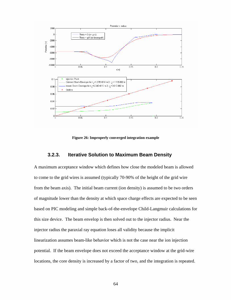
Figure 25: Improperly converged integration example .................................................... 64 Figure 26: Potential map (top) and beam envelope (bottom) versus beam-line position for
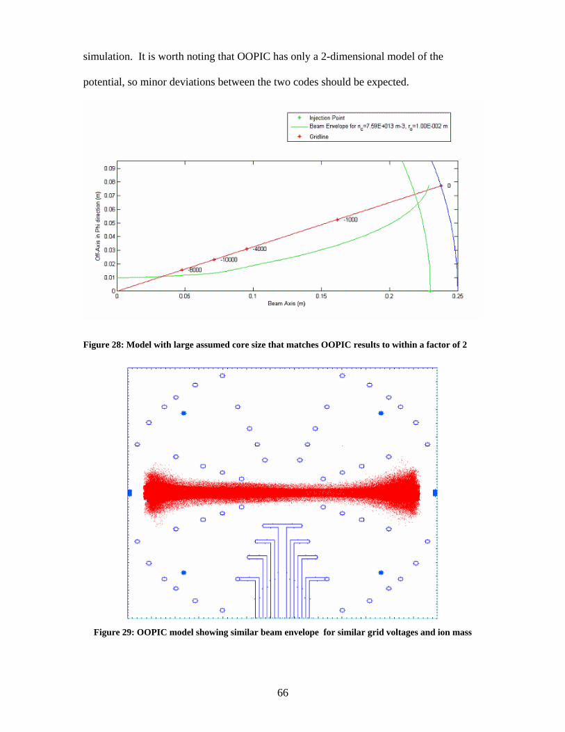
very small core focus and high core ion density (not reproducible in OOPIC)........ 65 Figure 27: Model with large assumed core size that matches OOPIC results to within a
factor of 2.................................................................................................................. 66 Figure 28: OOPIC model showing similar beam envelope for similar grid voltages and
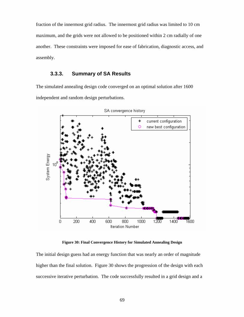
ion mass .................................................................................................................... 66 Figure 29: Final Convergence History for Simulated Annealing Design......................... 69 Figure 30: Number of occurrences v. energy in final SA run........................................... 70 Figure 31: Evolution of the SA design showing the freezing of the configuration .......... 71
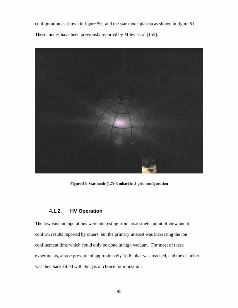
8
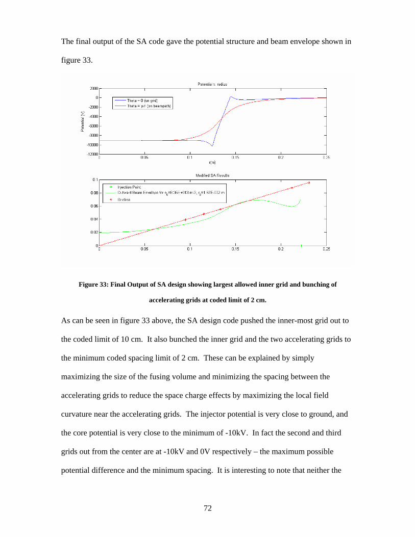
Figure 32: Final Output of SA design showing largest allowed inner grid and bunching of accelerating grids at coded limit of 2 cm. ................................................................. 72
Figure 33: Low pressure, 2-grid OOPIC simulation, ion injector on ............................... 75 Figure 34: Time evolution of Argon +1 ions in the simplest 2-grid OOPIC model (no
background gas) ........................................................................................................ 76 Figure 35: 2-Grid OOPIC model showing ions impacting cathode after 1/2 to 5 passes. 78 Figure 36: Typical simulated multi-grid geometry, x and y dimensions are meters, grid
locations and ion injector geometry are based upon the physical experiment......... 80 Figure 37: Typical plot of number of macroparticles in an OOPIC simulation ............... 80 Figure 38: OOPIC multi-grid potential model for a scenario with good ion confinement81 Figure 39: Symmetric multi-grid field with poorly confined ions.................................... 82 Figure 40: Comparison of perfectly symmetric field (left) with a 2.5% location
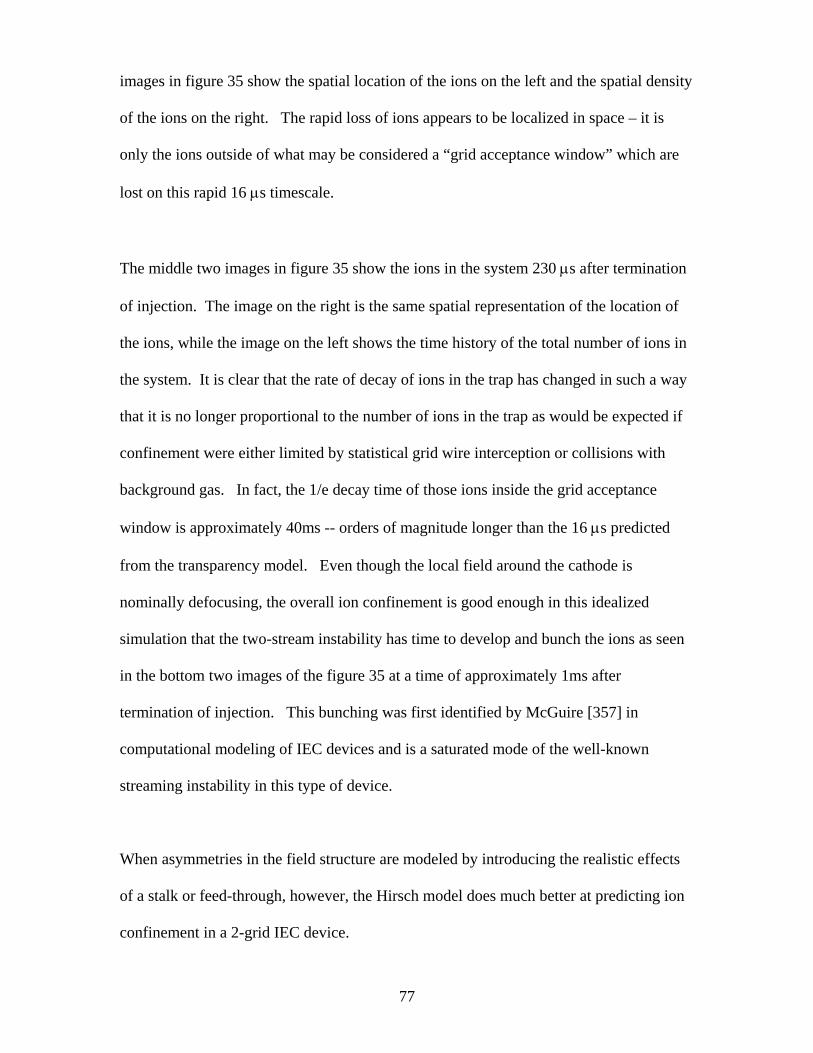
perturbation on one wire (right). The perturbed wire is the second grid from the center in the upper left hand quandrant..................................................................... 83
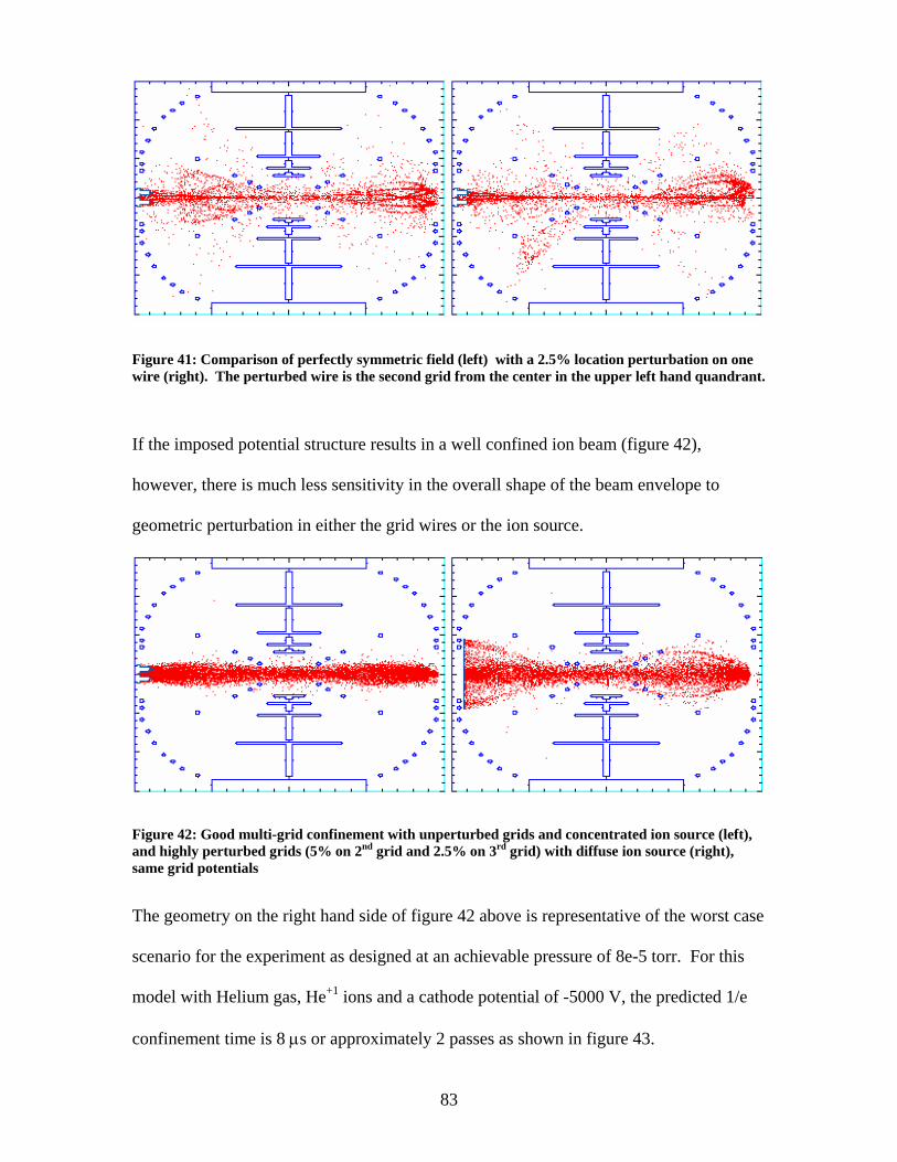
Figure 41: Good multi-grid confinement with unperturbed grids and concentrated ion source (left), and highly perturbed grids (5% on 2nd grid and 2.5% on 3rd grid) with diffuse ion source (right), same grid potentials ........................................................ 83
Figure 42: Normalized plot of the decay of the number of ions in the "worst case" OOPIC simulation for 8e-5 mbar He. .................................................................................... 84
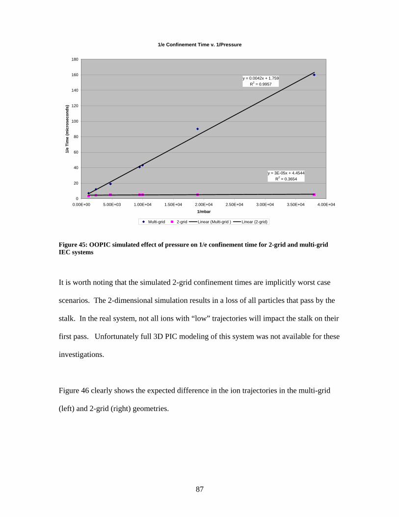
Figure 43: Normalized decay curve of best case, Helium at 8e-5 torr ............................. 85 Figure 44: OOPIC simulated effect of pressure on 1/e confinement time for 2-grid and
multi-grid IEC systems ............................................................................................. 87 Figure 45: Multi-grid (left) and 2-grid (right) OOPIC simulations .................................. 88 Figure 46: Non-exponential decay shape of multi-grid in perfect vacuum ...................... 89 Figure 47: Predicted sensitivity of 1/e confinement time to 3rd grid potential (1e-4 mbar)
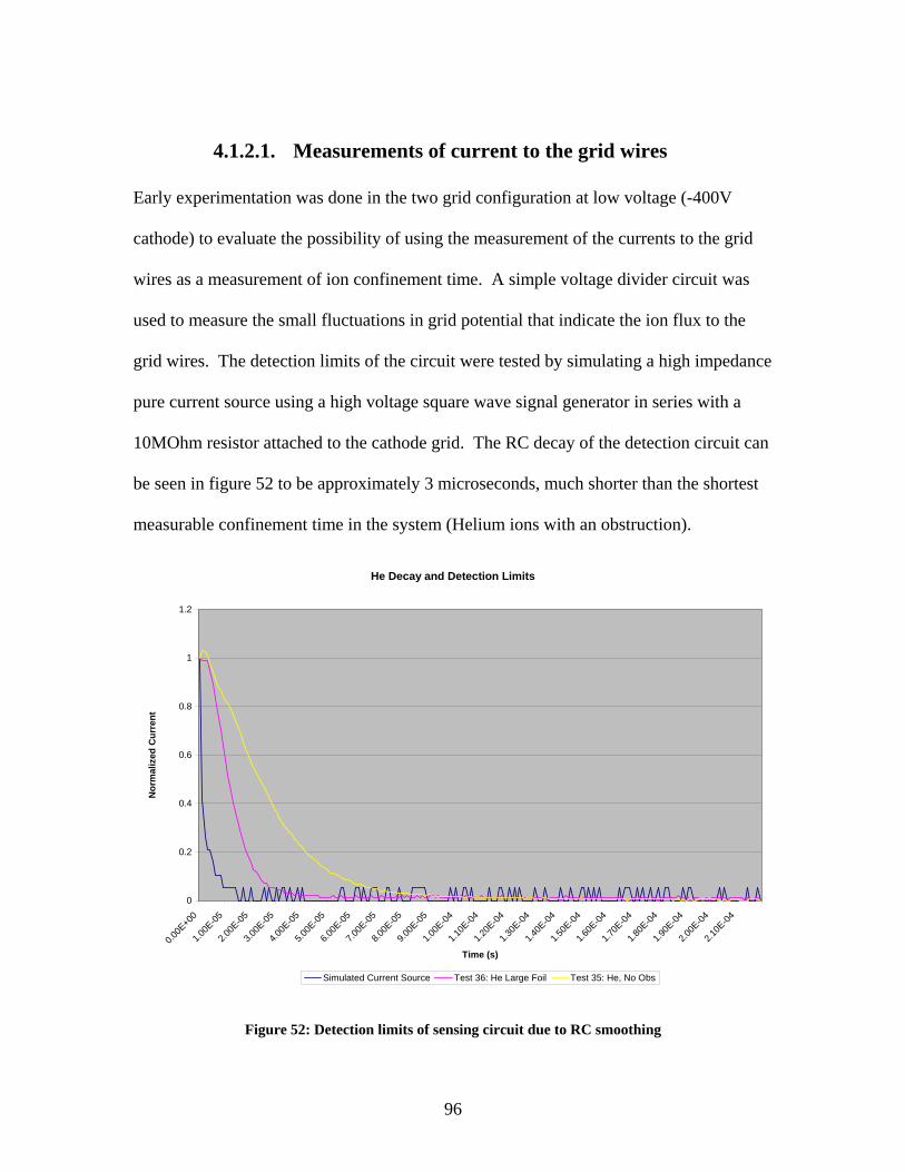
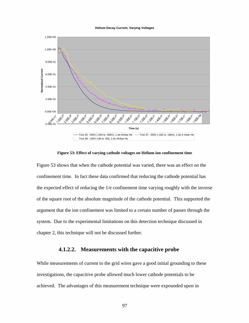
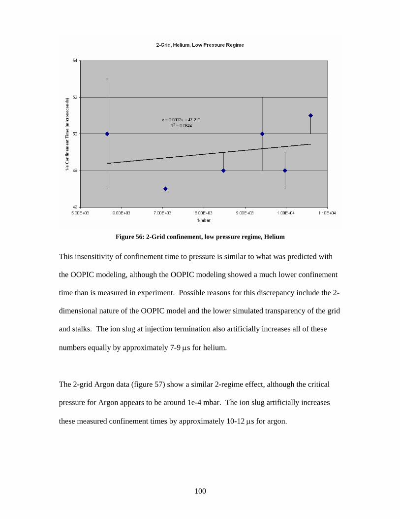
................................................................................................................................... 90 Figure 48: 2-Grid assembly in the vacuum chamber ........................................................ 93 Figure 49: Jet-mode in 2-grid configuration..................................................................... 94 Figure 50: Star mode (1.7e-3 mbar) in 2-grid configuration ............................................ 95 Figure 51: Detection limits of sensing circuit due to RC smoothing................................ 96 Figure 52: Effect of varying cathode voltages on Helium ion confinement time............. 97 Figure 53: Effect of pressure on 2-grid confinement, Helium.......................................... 98 Figure 54: 2-Grid confinement, high pressure regime, Helium........................................ 99 Figure 55: 2-Grid confinement, low pressure regime, Helium....................................... 100 Figure 56: 2-Grid confinement time pressure sensitivity, Argon ................................... 101 Figure 57: 2-Grid high pressure regime, Argon.............................................................. 102 Figure 58: 2-Grid low pressure regime, Argon............................................................... 102 Figure 59: Multi-grid discharge 2e-2 mbar, air .............................................................. 105 Figure 60: Many jets (~1.5e-2 mbar) .............................................................................. 106 Figure 61: Multi-grid air discharge 1e-2 mbar ............................................................... 106 Figure 62: Multi-grid jet-mode (7e-3 mbar) ................................................................... 107 Figure 63: Multi-grid “jumping” jet exposure ................................................................ 107 Figure 64: Multi-grid, star-mode 3e-3 mbar, air............................................................. 108 Figure 65: 1/e Confinement time v. 1/Pressure, Helium ................................................ 110 Figure 66: Pressure effect: comparing experimental results to OOPIC, Helium............ 110 Figure 67: Multi-grid Helium ion decay curve, 1e-4 mbar............................................. 112 Figure 68: Multi-grid Argon ion decay curve, 1.0e-4 mbar ........................................... 113 Figure 69: Multi-grid Argon Confinement Pressure Sensitivity..................................... 114
9
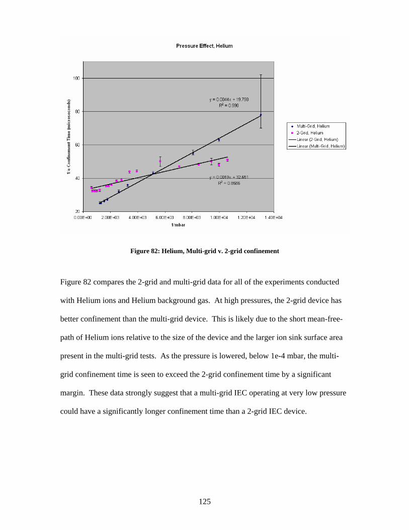
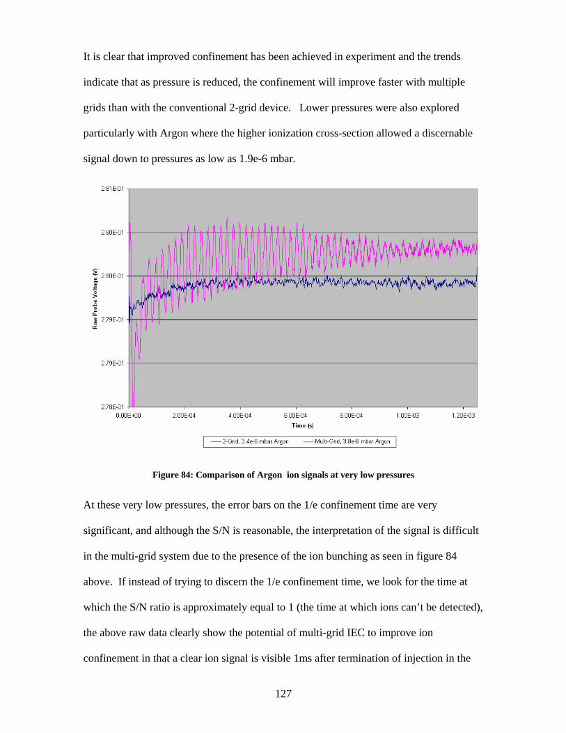
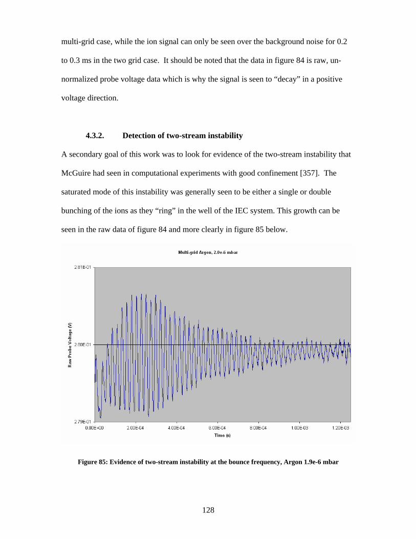
Figure 70: Higher pressure regime decay example......................................................... 115 Figure 71: Lower pressure regime decay example ......................................................... 115 Figure 72: High pressure confinement regime, Argon ................................................... 116 Figure 73: Low pressure confinement regime, Argon .................................................... 117 Figure 74: Voltage sweep comparison to OOPIC simulation......................................... 118 Figure 75: 2nd Grid voltage sweep, Helium................................................................... 120 Figure 76: 2nd Grid voltage sweep, Argon..................................................................... 120 Figure 77: 3rd grid voltage sweep, Helium .................................................................... 121 Figure 78: 3rd grid voltage sweep, Argon ...................................................................... 121 Figure 79: 4th grid sweep, Helium ................................................................................. 122 Figure 80: 4th grid sweep, Argon ................................................................................... 122 Figure 81: Helium, Multi-grid v. 2-grid confinement..................................................... 125 Figure 82: Argon, Multi-grid v. 2-grid confinement ...................................................... 126 Figure 83: Comparison of Argon ion signals at very low pressures.............................. 127 Figure 84: Evidence of two-stream instability at the bounce frequency, Argon 1.9e-6
mbar ........................................................................................................................ 128 Figure 85: Normalized oscillation envelope and exponential-sigmoid curve fit for the test
plotted in figure 84 (Argon, 1.9e-6 mbar)............................................................... 130
10
1. Introduction
1.1. Background
Inertial electrostatic confinement (IEC) fusion is often credited as being conceived of by
Philo T. Farnsworth, the inventor of television [20]. In IEC devices, fusion ions are
electrostatically accelerated through a (nearly) spherically symmetric central focus point.
At the focus point they are at sufficiently high energy to overcome their mutual
electrostatic repulsion that some small fraction of the ions will fuse and release energy in
the form of high energy fusion products. Figure 1 illustrates the practical simplicity of
IEC fusion.
Figure 1: Schematic drawing of conventional, 2-grid IEC device
11
The earliest published work on the concept was done by Salisbury in 1949 [1], then
expanded by Elmore, Tuck and Watson in the late 1950s[2, 3]. There has been sporadic
work on IEC fusion for the past 50 years [4-350]. Experimental programs are relatively
cheap to develop, and they have been shown to be a detectable neutron source given
sufficient input power. The largest fusion output to date was achieved by Hirsch in 1967
with an output of nearly 1010 neutrons/second with Deuterium and Tritium [18]. It is
widely accepted that it is not difficult to make fusion reactions in an IEC reactor, but the
best efficiency to date as measured by the fusion power out divided by the electrical
power in (Q) is approximately 10-5. Because of its poor efficiency, IEC has never been a
priority in the quest for a fusion energy source.
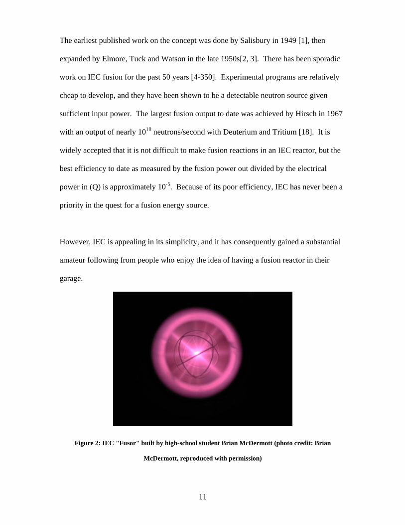
However, IEC is appealing in its simplicity, and it has consequently gained a substantial
amateur following from people who enjoy the idea of having a fusion reactor in their
garage.
Figure 2: IEC "Fusor" built by high-school student Brian McDermott (photo credit: Brian
McDermott, reproduced with permission)
12
These devices have developed a strong following in online forums and bulletin boards.
Figure 2 is a photograph of an operating IEC fusion reactor built by high school student,
Brian McDermott. Many other amateur scientists have built similar “fusor reactors”
[361].
Theoretical systems studies have identified significant barriers to the practical
implementation of IEC fusion systems for power production [175], but significant interest
remains because of the simplicity, the attractive scaling, and the low mass of the IEC
fusion reactor system. This low mass is particularly of interest for space-based power
and propulsion systems. While there are designs for many types of magnetically
confined and inertial fusion reactors that are much closer to achieving net power output,
these concepts are sufficiently massive that tremendous monetary resources would need
to be allocated for development of that type of reactor in space. The scale of such an
undertaking would likely surpass the scale of the International Space Station (ISS) –
requiring multiple launches and in-space assembly. It is therefore valuable to work on
the challenges associated with making IEC fusion more efficient because of the potential
to put an entire reactor in space with a single launch. The potential for a more practical,
small-scale, implementation of fusion power for spacecraft systems is the fundamental
driver for this research.
The primary limiter of the efficiency of IEC fusion systems is the extremely short energy
confinement time, the embodiment of which is the short charged particle confinement
time in the system. Under typical IEC operating parameters, electrons stream out from
13
the central cathode and are collected on the outer anode, and ions typically make only 10
passes through the cathode before being lost by either impacting one of the grid wires or
undergoing a charge-exchange reaction with background gas in the system [357]. In a
typical system, the probability that any given ion will be lost to a process other than
fusion is approximately 100,000 times more likely than losing an ion to a fusion reaction.
Previous work [357] identified the need to operate an IEC fusion device in a regime
where the ion loss probability is within the fusion energy gain to input power ratio of ion
fusion probability (a factor of order 10) in order to approach Q=1. The improvement of
charged particle confinement in IEC systems is therefore of paramount interest. Sedwick
and McGuire proposed a method of improving ion confinement times by electrostatically
focusing ion beams to keep them away from cathode grid wires. McGuire also identified
the need to operate the system in the ultra-high-vacuum (UHV) regime in order to avoid
charge-exchange and collisional scattering losses with background gas. With an
appropriately hard vacuum and a properly focused recirculating ion beam, typical ion
confinement times were computationally shown to be improvable by three orders of
magnitude – from 10 passes to 10,000 passes dependent on the background pressure.
This improved ion confinement has the potential to yield dramatic improvements in
system efficiency [357].
The practical implementation of this type of improved confinement requires the
development of an IEC reactor with 3 or more independently biased, concentric spherical
grids (multi-grid). The potentials on these grids would be set so as to provide a confining
electrostatic field. By minimizing the rate of ion-grid impact, the electron current will
14
also be reduced because the majority of streaming electrons are emitted as secondary
electrons when ions collide with the cathode. Electrostatic ion confinement thereby has
the potential to reduce the two largest energy sinks in IEC systems.
While focusing ion beams is nothing new to physicists, and there are many tools to
predict ion beam behavior in the presence of focusing fields, the development of new
models was required in order to predict the behavior of ions in this type of recirculating
ion trap. The development of some of those new models and the construction and
experimental evaluation of the first multi-grid IEC confinement experiment is the subject
of this thesis.
1.2. Rationale Behind Current Investigations
Previous work computationally identified the potential to improve ion confinement in
IEC devices by implementing a multiple-grid configuration, but hardware based tests
were needed to experimentally validate the predicted improvement.
1.2.1. Ion Confinement
The goal of this research is to compare a conventional, 2-grid IEC device with a 5-grid
IEC device to evaluate the potential of the multi-grid approach to improve ion
confinement. Based on the computational modeling, significant increases in ion
confinement were expected with properly tailored potentials in the 5-grid device. The
major ion loss mechanisms in a conventional, 2-grid IEC device are chaotic ion
trajectories and background gas interactions. Operating the 5-grid device at very low
background gas pressure and with a focusing field structure is expected to improve ion
confinement.
15
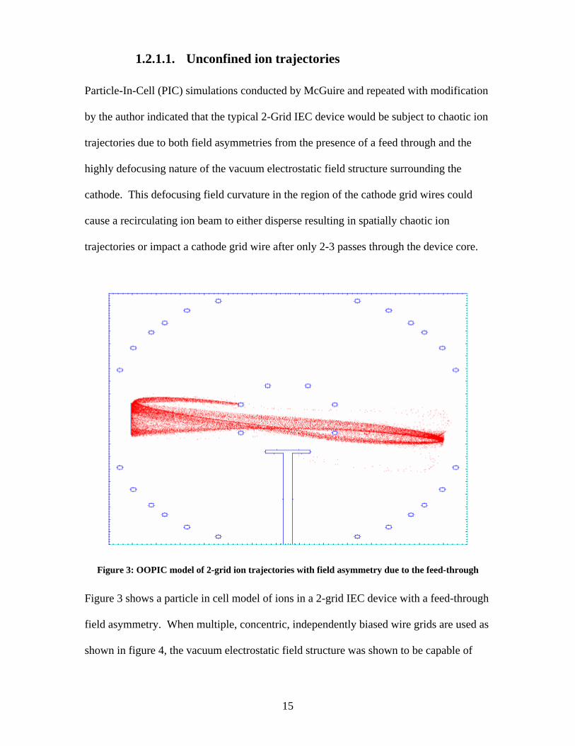
1.2.1.1. Unconfined ion trajectories
Particle-In-Cell (PIC) simulations conducted by McGuire and repeated with modification
by the author indicated that the typical 2-Grid IEC device would be subject to chaotic ion
trajectories due to both field asymmetries from the presence of a feed through and the
highly defocusing nature of the vacuum electrostatic field structure surrounding the
cathode. This defocusing field curvature in the region of the cathode grid wires could
cause a recirculating ion beam to either disperse resulting in spatially chaotic ion
trajectories or impact a cathode grid wire after only 2-3 passes through the device core.
Figure 3: OOPIC model of 2-grid ion trajectories with field asymmetry due to the feed-through
Figure 3 shows a particle in cell model of ions in a 2-grid IEC device with a feed-through
field asymmetry. When multiple, concentric, independently biased wire grids are used as
shown in figure 4, the vacuum electrostatic field structure was shown to be capable of
16
confining the ions away from the cathode grid wires for many more passes through the
core than in the conventional, 2-grid design simulated above. With the confining field
structure of the multi-grid configuration, significant improvements in ion confinement
were shown to be possible even with a small, off-axis ion injector that would act as an ion
sink as well as a source.
Figure 4: Multi-grid with asymmetric feed-through and off-axis, absorbing ion injector
These early studies strongly indicated that uncontrolled ion trajectories in conventional,
2-grid IEC devices could be a major ion (and energy) loss mechanism and supported the
hypothesis that the use of multiple grids could significantly improve ion (and energy)
confinement times in IEC devices.
17
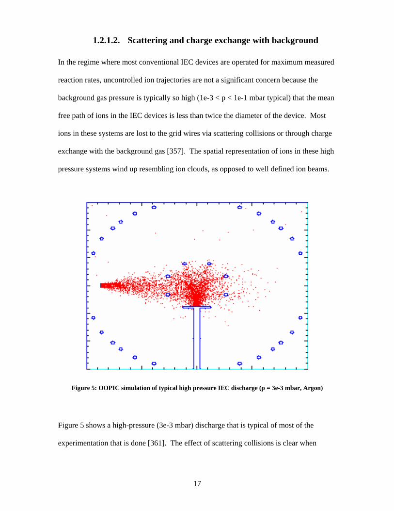
1.2.1.2. Scattering and charge exchange with background
In the regime where most conventional IEC devices are operated for maximum measured
reaction rates, uncontrolled ion trajectories are not a significant concern because the
background gas pressure is typically so high (1e-3 < p < 1e-1 mbar typical) that the mean
free path of ions in the IEC devices is less than twice the diameter of the device. Most
ions in these systems are lost to the grid wires via scattering collisions or through charge
exchange with the background gas [357]. The spatial representation of ions in these high
pressure systems wind up resembling ion clouds, as opposed to well defined ion beams.
Figure 5: OOPIC simulation of typical high pressure IEC discharge (p = 3e-3 mbar, Argon)
Figure 5 shows a high-pressure (3e-3 mbar) discharge that is typical of most of the
experimentation that is done [361]. The effect of scattering collisions is clear when
18
compared to the hard vacuum of figure 2. In this high pressure regime, the majority of
fusion reactions are between ions and the neutral background gas. While the measurable
neutron output is highest in this pressure regime, the scattering and charge exchange
interactions of the ions with the background gas limits the ion confinement time. The
maximum measured Q of IEC devices in this high pressure regime approached 10-5 with
deuterium and tritium (DT reaction) gas [18]. IEC operation in most experiments uses
only deuterium (DD reaction). The average Q is of the order 10-9.
1.2.2. OOPIC Modeling
A Particle-In-Cell (PIC) modeling tool has been developed using a commercial-off-the-
shelf (COTS) code called OOPIC. The OOPIC physics kernel was originally developed
by UC Berkeley’s computational physics group [359, 360]. It is a 2-D code that has a
wide range of built in functionality including a Monte Carlo Collision (MCC) model,
simulated ion sources, realistic electron and ion bombardment ionization models for
Argon, Helium and a number of other gases, and simple user definable geometries.
PIC modeling informed much of the original investigations into improving ion
confinement. It has been particularly useful for predicting ion bounce times, simulating
the effects of multiple grids, and evaluating the development of the ion-ion counter-
streaming instability in these low-pressure, non-neutral IEC systems with good particle
confinement.
19
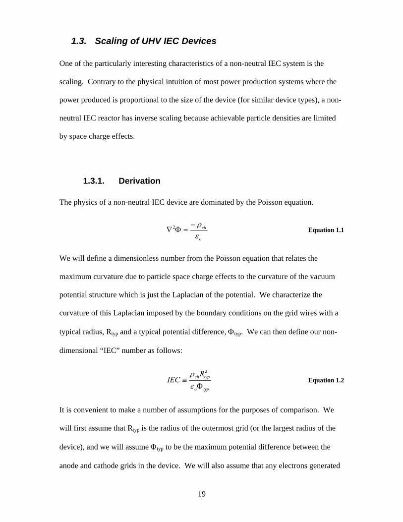
1.3. Scaling of UHV IEC Devices
One of the particularly interesting characteristics of a non-neutral IEC system is the
scaling. Contrary to the physical intuition of most power production systems where the
power produced is proportional to the size of the device (for similar device types), a non-
neutral IEC reactor has inverse scaling because achievable particle densities are limited
by space charge effects.
1.3.1. Derivation
The physics of a non-neutral IEC device are dominated by the Poisson equation.
o
ch
ερ−
=Φ∇2 Equation 1.1
We will define a dimensionless number from the Poisson equation that relates the
maximum curvature due to particle space charge effects to the curvature of the vacuum
potential structure which is just the Laplacian of the potential. We characterize the
curvature of this Laplacian imposed by the boundary conditions on the grid wires with a
typical radius, Rtyp and a typical potential difference, Φtyp. We can then define our non-
dimensional “IEC” number as follows:
typo
typchRIEC
Φ≡
ερ 2
Equation 1.2
It is convenient to make a number of assumptions for the purposes of comparison. We
will first assume that Rtyp is the radius of the outermost grid (or the largest radius of the
device), and we will assume Φtyp to be the maximum potential difference between the
anode and cathode grids in the device. We will also assume that any electrons generated
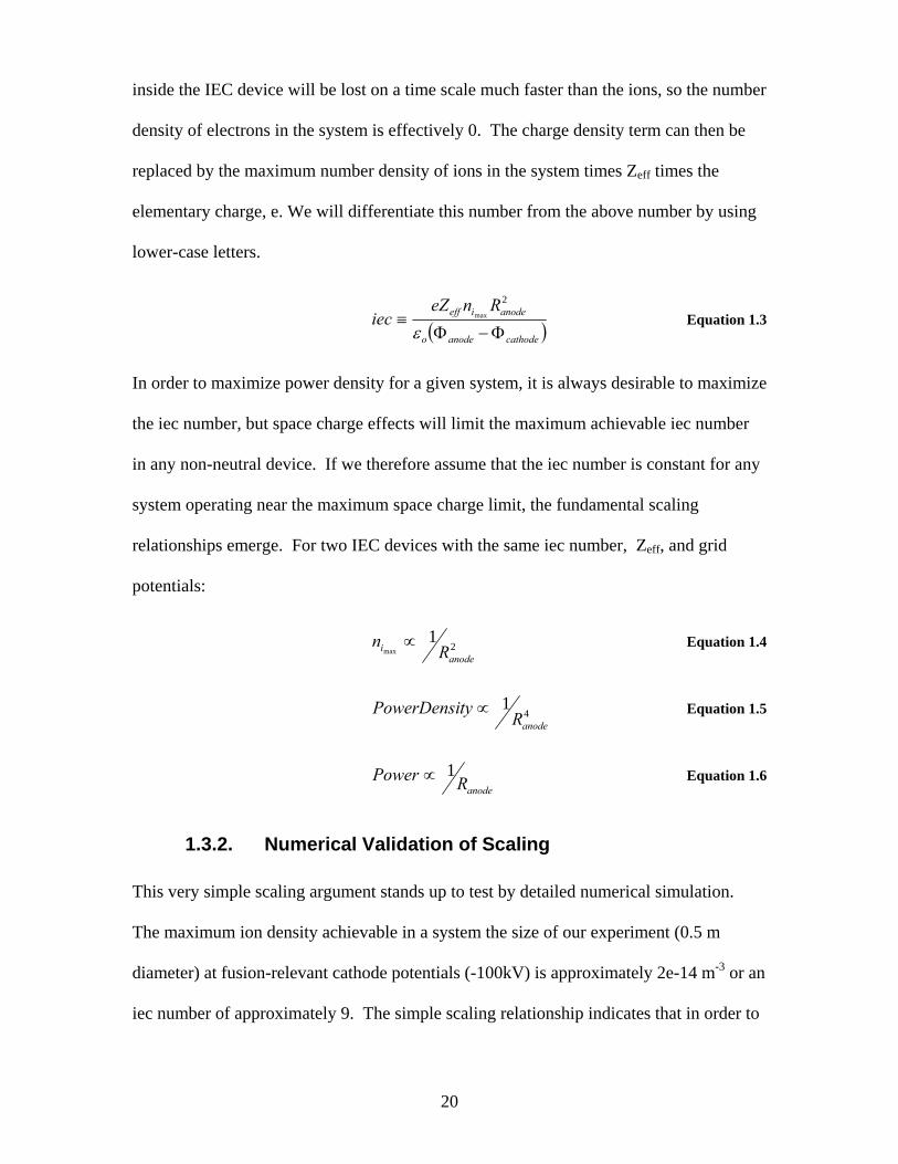
20
inside the IEC device will be lost on a time scale much faster than the ions, so the number
density of electrons in the system is effectively 0. The charge density term can then be
replaced by the maximum number density of ions in the system times Zeff times the
elementary charge, e. We will differentiate this number from the above number by using
lower-case letters.
( )cathodeanodeo
anodeieff RneZiec
Φ−Φ≡
ε
2max Equation 1.3
In order to maximize power density for a given system, it is always desirable to maximize
the iec number, but space charge effects will limit the maximum achievable iec number
in any non-neutral device. If we therefore assume that the iec number is constant for any
system operating near the maximum space charge limit, the fundamental scaling
relationships emerge. For two IEC devices with the same iec number, Zeff, and grid
potentials:
21
maxanode
i Rn ∝ Equation 1.4
41
anodeRtyPowerDensi ∝ Equation 1.5
anodeRPower 1∝ Equation 1.6
1.3.2. Numerical Validation of Scaling
This very simple scaling argument stands up to test by detailed numerical simulation.
The maximum ion density achievable in a system the size of our experiment (0.5 m
diameter) at fusion-relevant cathode potentials (-100kV) is approximately 2e-14 m-3 or an
iec number of approximately 9. The simple scaling relationship indicates that in order to
21
achieve ion densities that are comparable to those in a Tokamak, the radius of the device
must be decreased by a factor of 1000.
Figure 6: Particle-In-Cell simulation showing ni 2.5e20m-3 at 0.5mm diameter device size
When a geometrically similar OOPIC model was created with a diameter of 0.4 mm and
the same -100kV potential was applied to the cathode, the peak ion densities were seen to
top 2.5e20 m-3 (an iec number of 7.4) as predicted by the simple scaling derivation in the
previous section.
Although the maximum iec number for a given size system does depend on the details of
the design and implementation, for a system with good ion confinement that approaches
its own space charge limits, the iec numbers are not expected to vary by more than one
order of magnitude because fundamental space charge limits cannot be designed around
in non-neutral systems.
22
2. Experiment Development
Experimental validation of the hypothesis that ion confinement time in IEC devices could
be improved by the addition of wire focusing grids was sought. It was decided at an early
stage that this experimental validation would come from the simple geometric
reconfiguration of the wire grids in a single experiment at high vacuum. The experiment
would first be built in a conventional 2-grid geometry with a single cathode grid near the
center of a much larger anode grid such as the geometries represented in figures 3 and 5.
The ion confinement times for this system would be inferred from measured data.
Additional focusing grids would then be added to the system (similar to figure 4), and ion
confinement times would again be inferred from the new, “Multi-grid” data. These two
data sets would then be compared to reveal whether they support the core hypothesis.
A number of design and modeling techniques were employed to facilitate the design of
the experiment. These models are detailed in the following chapter. The net result of the
modeling effort was to confirm assertions that were inferred from the basic scaling given
in chapter one and, more importantly, to quantify and predict the expected ion densities
and confinement times of the system.
The geometry of the experiment was largely dictated by experimental convenience –
available equipment, measurement access, and ease of grid construction with available
tools and techniques. This section discusses four critical aspects of the development of
the experiment: confinement time detection techniques, sources of error, selection of
primary diagnostic, and hardware development.
23
2.1. Confinement Time Detection Techniques
There are many ways to measure the confinement time of ions in an IEC system. This
section will give an overview of the concepts that were considered for this experiment.
All of the techniques presented require that the source of ions have either a well
calibrated injection rate or a rapid on/off switching time. If neither of these conditions
can be met, accurate measurement of the ion confinement time is not possible.
2.1.1. Measurement of current to the grid wires
As ions are injected into an IEC system where wire grids are used to establish the
background potential structure, they will occasionally adopt a trajectory that will
intercept one of the grid wires. When an ion impacts a grid wire it is rapidly decelerated
and neutralized by the “sea” of electrons in the wire. In the process, the energy of the ion
goes into heating the grid wire and potentially liberating secondary electrons from the
surface of the wire. Because the ion is neutralized on the surface, the impact of an ion on
a grid wire will draw an electric current which can be detected. The current drawn will
be proportional to, but not identical to the ion current (defined by the rate of ion loss
times the charge per ion). This discrepancy is due to the emission of secondary electrons
from the surface of the wire which will cause the detected current to exceed the ion loss
current by the average secondary electron yield factor.
( )ieionsgrid II γ+= 1 Equation 2.1
Early particle-in-cell (PIC) experiments showed that the number of ions lost to grid wires
per unit time is roughly proportional to the number of ions trapped in the system at that
time, particularly under high vacuum conditions where confinement limits are imposed
24
by collisions with background gas. Once the source of ions in turned off, this
relationship will cause the rate of ion loss to follow an exponential decay curve. One
method of estimating the confinement time of ions in the system is to numerically
evaluate the time-constant of the assumed exponential decay. This can be done by
measuring the time between the maximum loss rate and 1/e times that loss rate after the
ion source has been turned off. In this manner, ion confinement time can be inferred
from the measurement of the current to the grid wires as a function of time.
2.1.2. Destructive Beam Dump
Ion confinement time can be directly measured by a destructive count of the number of
ions remaining in the trap a certain period of time after ion injection is turned off. This
technique is referred to as a destructive beam dump (DBD). The DBD hardware would
consist of an ion collector plate mounted in the beam path near the anode opposite the ion
source. The collector plate would be held at or near ground so that ions could not impact
the plate without substantial upscatter or thermalization of the distribution function.
Then, when a measurement of the trapped ion population is desired, the potential of the
plate would be rapidly lowered so that all of the ions would be energetically capable of
impacting the collector plate. The location of the plate inline with the beam will cause all
of the ions in the trap to be rapidly evacuated and neutralized on the surface of the
collector. If the gradient of the electrostatic potential at the surface of the plate is such
that it suppresses any net secondary electron emission, the time integral of the current
that is drawn to the plate will be equal to the net charge that had been contained in the
trap. When this measurement is made in conjunction with assumptions about the relative
fraction of singly and doubly ions, the total population of ions in the trap at the dump
time could be inferred with a high level of confidence.
25
DBD is appealing because it has the potential to be a direct measurement of the total
trapped ion population at a given time. By taking many of these measurements with
different delays from the termination of ion injection, a decay curve can be extracted of
the actual ion population in the trap. Although many more measurements are required to
perform this analysis, it is appealing in that the actual number of ions is measured as
opposed to a signal that is simply proportional to the actual number of ions (as in the
previous technique).
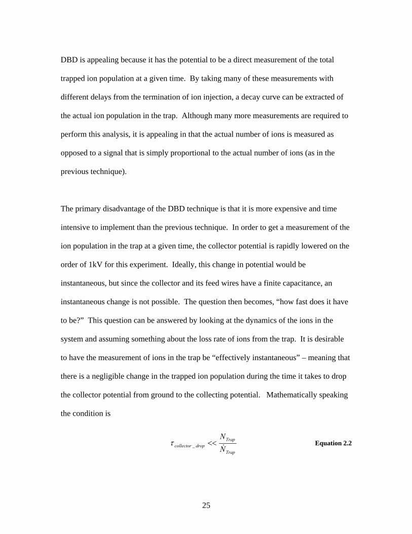
The primary disadvantage of the DBD technique is that it is more expensive and time
intensive to implement than the previous technique. In order to get a measurement of the
ion population in the trap at a given time, the collector potential is rapidly lowered on the
order of 1kV for this experiment. Ideally, this change in potential would be
instantaneous, but since the collector and its feed wires have a finite capacitance, an
instantaneous change is not possible. The question then becomes, “how fast does it have
to be?” This question can be answered by looking at the dynamics of the ions in the
system and assuming something about the loss rate of ions from the trap. It is desirable
to have the measurement of ions in the trap be “effectively instantaneous” – meaning that
there is a negligible change in the trapped ion population during the time it takes to drop
the collector potential from ground to the collecting potential. Mathematically speaking
the condition is
Trap
Trapdropcollector N
N&
<<_τ Equation 2.2
26
PIC modeling of the system suggests that the confinement time of a 2-grid system is
O(10) passes. Since it is desirable to compare the 2-grid system with the multi-grid
system using the same diagnostic, the characteristic time for the collector potential drop
( dropcollector _τ ) should be less than half of the bounce time in order for accurate
measurements of the 2 grid confinement time with a DBD technique.
2_b
dropcollectorττ < Equation 2.3
In addition, there is concern that the 2-grid beamline is not robust to minor asymmetries
in the potential structure which could cause the beam to intersect the collector plate near
the edge or miss the plate entirely. Clearly, if the plate is missed entirely, an accurate
measurement cannot be made with this technique, but even if the beam impacts the
collector near the edge, secondary electrons could be emitted from the collector to the
ground which would introduce error into the “direct” measurement of trapped ions.
There are other practical difficulties with implementing this type of detection scheme.
The current required to change the potential of the plate due to its finite capacitance
would need to be subtracted from the signal, and the need to rapidly pulse the potential of
the collector over the very short dump time requires special power supplies.
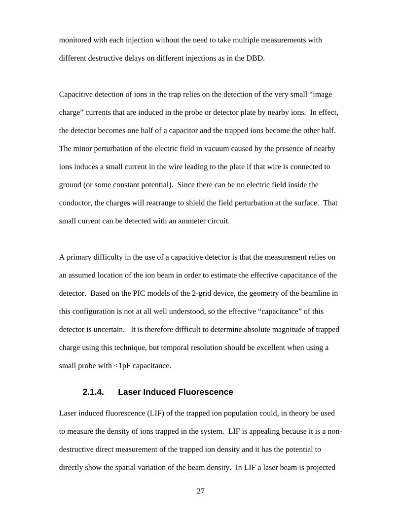
2.1.3. Capacitive Detection of Trapped Charge
A probe or plate like the one used as a collector in the DBD technique can be similarly
used to detect the trapped ions capacitively. Not only is this a direct measurement of the
ions in the trap, it is also a non-destructive measurement so the entire decay can be
27
monitored with each injection without the need to take multiple measurements with
different destructive delays on different injections as in the DBD.
Capacitive detection of ions in the trap relies on the detection of the very small “image
charge” currents that are induced in the probe or detector plate by nearby ions. In effect,
the detector becomes one half of a capacitor and the trapped ions become the other half.
The minor perturbation of the electric field in vacuum caused by the presence of nearby
ions induces a small current in the wire leading to the plate if that wire is connected to
ground (or some constant potential). Since there can be no electric field inside the
conductor, the charges will rearrange to shield the field perturbation at the surface. That
small current can be detected with an ammeter circuit.
A primary difficulty in the use of a capacitive detector is that the measurement relies on
an assumed location of the ion beam in order to estimate the effective capacitance of the
detector. Based on the PIC models of the 2-grid device, the geometry of the beamline in
this configuration is not at all well understood, so the effective “capacitance” of this
detector is uncertain. It is therefore difficult to determine absolute magnitude of trapped
charge using this technique, but temporal resolution should be excellent when using a
small probe with <1pF capacitance.
2.1.4. Laser Induced Fluorescence
Laser induced fluorescence (LIF) of the trapped ion population could, in theory be used
to measure the density of ions trapped in the system. LIF is appealing because it is a non-
destructive direct measurement of the trapped ion density and it has the potential to
directly show the spatial variation of the beam density. In LIF a laser beam is projected
28
through a measurement region that is anticipated to contain an ion population. The laser
is tuned to excite a particular electron transition. The decay of that excited ion releases a
photon in any direction. An aperture/filter arrangement in conjunction with a
photomultiplier tube is then used to detect some small fraction of these photons. That
signal is then assumed to be proportional to the density of ions in the region of space that
is intersected by the beam and the field of view of the detector. By monitoring the density
as a function of time (which may need to be done statistically with multiple
measurements because of the small signal) it is theoretically possible to back out the
trapped ion decay curve and hence the confinement time.
Due to the expense associated with the development of a LIF detector, LIF was never
seriously considered as a practical detection option for this experiment. It is mentioned
here because it has substantial promise to reveal the shape of the actual beam envelope
which could powerfully inform future investigations by validating or invalidating much
of the PIC modeling that has been done.
2.2. Sources of Error
Every experiment has many potential sources of error which at best introduce inaccuracy
or noise into the data and at worst cause the experiment to completely fail to measure
what it is attempting to measure. This section details a number of the potential sources of
error in what is anticipated to be levels of increasing significance.
2.2.1. Earth’s Magnetic Field
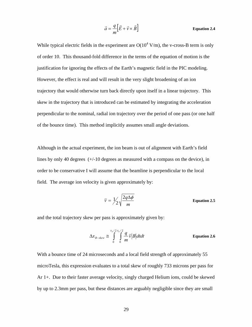
Charged particles will experience accelerations due to electric and magnetic fields.
29
[ ]BvEmqa
rrrr×+= Equation 2.4
While typical electric fields in the experiment are O(104 V/m), the v-cross-B term is only
of order 10. This thousand-fold difference in the terms of the equation of motion is the
justification for ignoring the effects of the Earth’s magnetic field in the PIC modeling.
However, the effect is real and will result in the very slight broadening of an ion
trajectory that would otherwise turn back directly upon itself in a linear trajectory. This
skew in the trajectory that is introduced can be estimated by integrating the acceleration
perpendicular to the nominal, radial ion trajectory over the period of one pass (or one half
of the bounce time). This method implicitly assumes small angle deviations.
Although in the actual experiment, the ion beam is out of alignment with Earth’s field
lines by only 40 degrees (+/-10 degrees as measured with a compass on the device), in
order to be conservative I will assume that the beamline is perpendicular to the local
field. The average ion velocity is given approximately by:
mqv φ∆
=2
21 Equation 2.5
and the total trajectory skew per pass is approximately given by:
∫ ∫≅∆ −
2/
0
2/
0
b b
dtdtBvmqx skewB
τ τ
Equation 2.6
With a bounce time of 24 microseconds and a local field strength of approximately 55
microTesla, this expression evaluates to a total skew of roughly 733 microns per pass for
Ar 1+. Due to their faster average velocity, singly charged Helium ions, could be skewed
by up to 2.3mm per pass, but these distances are arguably negligible since they are small
30
with respect to the grid openings at the anode (~18cm). It would require approximately
123 passes (or about 2.9 milliseconds) for a singly charged argon ion to move from the
center of the beam to an anode grid wire based solely upon this magnetic drift. A singly
charged Helium ion would require 39 passes or approximately 147 microseconds to drift
the same distance. Since confinement times have generally been limited to
approximately 10 passes, the effect of this magnetic drift will be ignored. Asymmetries
in the electric field are far more likely to cause significant perturbations of the ion
trajectories than magnetic drift.
While the impact on ion trajectories is negligible, the Earth’s magnetic field could
substantially alter the trajectories of secondary electrons. But since all magnetic lines
intersect the anode, even very low energy electrons with Larmor radii much smaller than
the device scale will wind up impacting the anode. Due to the broad energy spectrum of
secondary electrons, and the fast dynamics compared to the ions, electron confinement
was not modeled. It is expected to be poor.
In addition to directly impacting the particle trajectories in the experiment, the Earth’s
field could also produce a Hall-effect current in the voltage divider resistors which could
result in a local corona and flashover effect on the surface of the resistors. In order to
protect the voltage dividers from corona and flashover and to prevent unwanted leak
currents, the voltage dividers are potted in Silicon RTV. There is no evidence from the
experiment that suggests that this phenomenon is occurring.
31
Overall, the Earth’s magnetic field is not expected to introduce substantial error into the
measurement of the ion confinement time.
2.2.2. Secondary Electron Emission
In the commercial PIC code OOPIC, the Vaughn model is used to predict secondary
electron emission from the surface of the grid wires [353]. There is large uncertainty,
however, in how much of the energy of impacting ions results in secondary electrons
versus surface heating versus sputtering. A thorough literature search was conducted, and
the work of Szapiro and Rocca [355] was determined to be a good basis for our estimates
of secondary electron production.
Due to the possibility of a current cascade where secondary electrons from one grid wire
are accelerated and impact other focusing wires at high energy which then produce their
own secondary electrons, only the measurement of the current to the cathode grid will be
used as being truly proportional to the ion flux.
Since the cathode will be held at -10kV for both the 2-grid and multi-grid cases, Szapiro
and Rocca would estimate our secondary electron yield at roughly 3 electrons/ion for
10keV argon ions impacting a stainless steel wire. Our stainless steel longitude wires are
annealed in the atmosphere, however, there is an oxide layer covering the stainless steel
wire which is likely to substantially enhance the secondary electron current. The 304
stainless steel from which our wires are made is composed of Iron (66-74%), Chrome
(18-20%), and Nickel (8-10%) with trace amounts of other elements. Based on the
research of Allen, Dyke, Harris, and Morris [356] it is likely that the majority of the
oxide on the wire surface is iron oxide. Direct data for argon ions impacting oxidized
32
iron at relevant energies were not located, but secondary electron yield from other oxides
with 10keV argon ions could be as high as 6 to 9 electrons/ion (for Aluminum oxide and
magnesium oxide respectively)[355].
These yields are in stark contrast to the yields of secondary electrons off of clean, pure
metal surfaces which are typically less than 1 electron/ion and depend substantially on
ion incidence angle as well as energy and crystallographic orientation of the base metal
[354].
While there is a large amount of uncertainty in the actual yield of secondary electrons, the
secondaries will actually increase the measured current to the grid in proportion to the ion
flux (for the cathode). Therefore secondary emission will be simultaneously a source of
increased signal strength and increased signal noise. Due to the statistical nature of the
process and the high frequency of grid impacts and secondary emission, the signal
strength is expected to increase much more than the noise. Of course, the oxide layer on
the grids may sputter off which could cause the signal/noise to degrade with time as the
grids are sputtered clean. The time of this variation will undoubtedly be a function of the
depth of the oxide layer on the grids and the conditions at which the system is run
Ions can be lost via undetectable pathways: recombination, or ion neutralization on the
ion source itself. These loss mechanisms have not been modeled because they are
assumed to be negligible compared to the primary loss mechanisms already discussed. If
33
confinement is worse than expected, it may be worthwhile to model these other possible
loss mechanisms.
2.2.4. Equipment Limitations
The experiment described in this thesis was conducted in a vacuum chamber that was
consistently capable of a high vacuum base pressure on the order of 5e-7 mbar. The
lowest pressure achieved in the chamber after extensive cleaning and a 3 day pump-down
was 8e-8 mbar. The facility does not have provisions for bake-out or an ion pump for
UHV operation. While these base pressures should allow the demonstration of improved
confinement in the multi-grid configuration, the chamber is not currently capable of
achieving the base pressures identified [357] as necessary for ion-ion collision limited
confinement.
Figure 7: Schematic model of one high-voltage grid circuit
The four high voltage power supplies that control the grid potentials are also each limited
to a maximum current of approximately 425 µA and a potential of -10 kV. The
34
maximum power output of each of the four independent supplies is approximately 4W.
The geometry of the HV feed-through and the wire grids resulted in a built-in capacitance
of approximately 3pF as shown in figure 7. Because 1/e ion confinement times could be
as low as half the bounce time (or a minimum of around 3µs for Helium ions and a -10kV
cathode), the resistance between the grids and ground (R2+R3 in figure 7) could be at
most 1MΩ in order for the RC decay time constant to be lower than the decay time we
are trying to measure using the direct measurement of current to the grid wires. This
resistance limitation combined with the power/current limitations on the HV supplies
resulted in a minimum cathode voltage of only -400V for the grid-current diagnostic.
It should be noted that by floating (isolating) the potential of either the power supply
itself or a difference amplifier across R1 in figure 7 the current could be measured
without this restriction on the grid voltage. Due to practical constraints on isolating these
components in the existing laboratory environment, these options were not pursued.
The use of the destructive beam-dump diagnostic was prevented by the unavailability of a
second functional fast-switching HV supply. One is necessary to control the injection of
ions, and another would be required to dump the trap after a certain amount of time.
Only one functional fast-switch was available for the present investigations. A second
switch was on hand, but it stopped working before useful measurements could be made.
Differential pumping was not available, so it was not practical to maintain a substantial
pressure differential between the ion production region and the bulk of the chamber
volume. Therefore, the strength (current out) of the ion source is proportional to the
35
background gas pressure in the chamber. When the pressure is reduced to levels where
multiple order-of-magnitude improvements in 1/e confinement time are predicted by the
particle in cell models, the ion source is so weak that the signal to noise ratio is too low to
discern the 1/e confinement time from the data.
A final, and potentially quite important source of error arises from the construction of the
ion source itself. The ion source is contains a thoriated tungsten filament which serves as
an electron source. The filament is located outside the anode grid. A fine (~1cm
spacing) wire mesh screen covers the equatorial section of the anode. See figure 18 in
the next section for a schematic drawing of the ion source. The filament potential is
rapidly (<1µs) switched from the ground (anode) potential to -150V. Electrons emitted
by the filament are then accelerated toward the anode screen. Because the screen is 87%
transparent, the Hirsch formula [21] suggests that electrons will make 3.58 passes back
and forth through the screen before impacting one of the wires. Background gas in the
region is ionized via electron bombardment. Ions that are generated inside the anode grid
fall into the potential well of the device, while ions that are created outside the anode grid
are accelerated towards the filament and are expected to generally result in the production
of more secondary electrons. When the ion source is turned off the filament potential is
rapidly (<1µs) raised to ground. The electrons that are now “boiled off” the surface
thermionically do not have sufficient energy to ionize the background gas. The ion
source is effectively turned off. The possible source of error arises from ions that were
generated on the outside of the anode just before the filament potential was grounded.
Those ions may be extracted from their location outside the anode screen into the
potential well by field penetration from the inner grids through the screen. This situation
36
could result in a “slug” of ions born outside the anode entering the well after the filament
potential is raised to ground. This transient slug of ions could result in an increase in the
measured 1/e confinement time. There is evidence to suggest that this happens in the
experiment.
2.3. Selection of Primary Diagnostic
Although it was originally anticipated that the measurement of the current to the grid
wires would be the primary diagnostic for the experiment, the limitations described in the
previous section resulted in a change in primary diagnostic.
2.3.1. Diagnostic Comparison
The candidates for the primary diagnostic were: the measurement of the current to the
grid wires, the measurement of the current to a probe near the anode held at a potential
lower than the anode, and the capacitive pickup on the probe near the anode held at a
potential above the anode. As previously mentioned, DBD and LIF had been discounted
due to equipment limitations.
The measurement of the current to the grid wires is limited to cathode voltages of -400 V.
There was concern that with this relatively high cathode voltage and correspondingly
shallow potential well, electrons born on the filament at -150V could penetrate quite far
down into the potential well. The ions born in the well from the electron bombardment
of the background gas would then have a relatively broad energy spectrum compared to
the well depth. This sort of “spread ion source” was shown in OOPIC simulation to
37
result in less well confined ions. The birth location and potential of the ions was
observed to have an impact on the ion confinement time in the OOPIC simulation, so this
detection technique was not selected as a primary diagnostic. It is useful for purposes of
comparison however.
A probe inserted into the ion beam opposite the ion injector was used to make two other
types of diagnostics (see figure 19). When the probe is biased at a potential lower than -
150V, all ions in the system are energetically capable of being neutralized on the surface
of the probe. The probe at this potential can act like a separate “collector grid” and allow
the direct measurement of lost ion current similar to the measurement of the current to the
grid wires. This type of diagnostic is appealing due to the ability to disconnect the grid
voltages from the collector voltage. The cathode grid can be biased to a potential much
lower than the -400V limit of the previous diagnostic, and the time resolution on the
detector can be improved by the use of a diagnostic with a smaller inherent capacitance
(<1pF) and a lower resistance (<1MΩ). The very presence of the probe, however,
significantly perturbs the potential structure around it because the Debye length of the
system at the operating densities is significantly larger than the diameter of the device.
This situation is true for any non-neutral IEC device. The perturbation of the potential
field around the probe results in an asymmetry which has the ability to change the
confinement properties. The biggest disadvantage of the use of the probe in this manner
is that it introduces an intentional ion sink into the ion beam that would not exist in an
operating device. Due to the 2-D nature of the OOPIC code, the effect of the probe at
this potential could not be realistically modeled because in the simulation, every ion that
38
approached the probe would neutralize on the surface. While this scenario is not
physical, there is not a good way of quantifying the error with the existing tools.
When the same probe is biased slightly above the anode potential (+0.3V, figure 20), ions
born in the system are energetically incapable of impacting the probe. The ion sink is
removed. A significant asymmetry in the potential structure still exists, but OOPIC
modeling (which could be used in this case since no ions are lost to the probe) suggested
that a potential structure with good confinement would still tend to have good
confinement with the probe in the system on one side. The probe at this potential acts as
a capacitive pickup. Although the currents to the probe will be lower, the probe should
not significantly reduce the confinement time of ions in the system. This diagnostic was
therefore chosen as the primary diagnostic for these experiments.
2.4. Hardware Development
Significant effort went into the development of the facilities necessary to show the
potential for multiple grids to improve the ion confinement time in IEC systems. This
section details some of the important work should it need to be recreated in the future.
2.4.1. Vacuum Chamber Retrofitting
A stainless steel vacuum tank was acquired from another university where it had been
used for sputtering materials. The inside of the tank was blasted clean and a hinged door
was retrofitted. An additional port was added to the tank to accommodate the 1000 L/s
turbopump used for all high vacuum operation. A leaded-glass window was added to one
of the ports. A 10kV electrical feedthrough was added to supply the grids, along with a
39
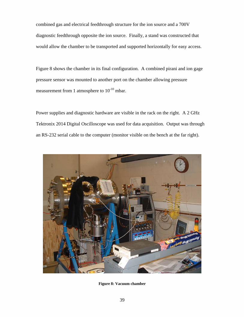
combined gas and electrical feedthrough structure for the ion source and a 700V
diagnostic feedthrough opposite the ion source. Finally, a stand was constructed that
would allow the chamber to be transported and supported horizontally for easy access.
Figure 8 shows the chamber in its final configuration. A combined pirani and ion gage
pressure sensor was mounted to another port on the chamber allowing pressure
measurement from 1 atmosphere to 10-10 mbar.
Power supplies and diagnostic hardware are visible in the rack on the right. A 2 GHz
Tektronix 2014 Digital Oscilloscope was used for data acquisition. Output was through
an RS-232 serial cable to the computer (monitor visible on the bench at the far right).
Figure 8: Vacuum chamber
40
2.4.2. Grid Fabrication
Since the decision had been made to construct the multi-grid portion of the experiment
with five concentric spherical wire grids, it was necessary to develop a standard
methodology for constructing the grids. The final solution that was arrived at is reported
in this section.
After considering many different options for grid wire materials, 1mm diameter 304
stainless steel wire was chosen for all grids so the structures would have sufficient
rigidity to survive normal handling, and so conventional, spot-welding techniques could
be implemented with ease. It is expected that a more detailed analysis of the material
choice will be required for future devices.
Figure 9: Fabrication of grid wire jig
41
A jig to hold the 304 stainless wire in place at the proper curvature for spot welding was
machined from a piece of polycarbonate as shown in figure 9. The wire was laid in the
trough and spot-welded to the desired diameters. It was then removed from the jig. The
wires that were to become longitude lines were then annealed so they could be cut and
still maintain the desired radius of curvature. After some limited experimentation shown
in figure 10, it was discovered that running a current of 35 A through the hoops for 1
minute would give the desired effect.
Figure 10: Grid wire annealing tests
When less current was used for less time, the wire would show some residual “spring-
back,” but if more current was used for much more time, the wire would tend to deform
significantly under its own weight and the forces applied by the alligator clips used to
supply the current.
42
Figure 11: Atmospheric annealing of longitude wires
Figure 11 shows the atmospheric annealing of one of the grid wires. Once the annealing
of the longitude lines was complete, they could be cut in sections and maintain the
desired radius of curvature. The latitude lines were not annealed because they did not
need to be cut during the assembly procedure. The longitude lines had to be cut so the
feed-throughs supplying the inner grids could pass through the pole and introduce the
minimum possible field asymmetry.
In order to attach the longitude wires to the polar feed-through, special stainless steel
rings were fabricated from 1/16” plate using an OMAX waterjet cutter. These rings
provided structural support and an electrical connection for the grids.
43
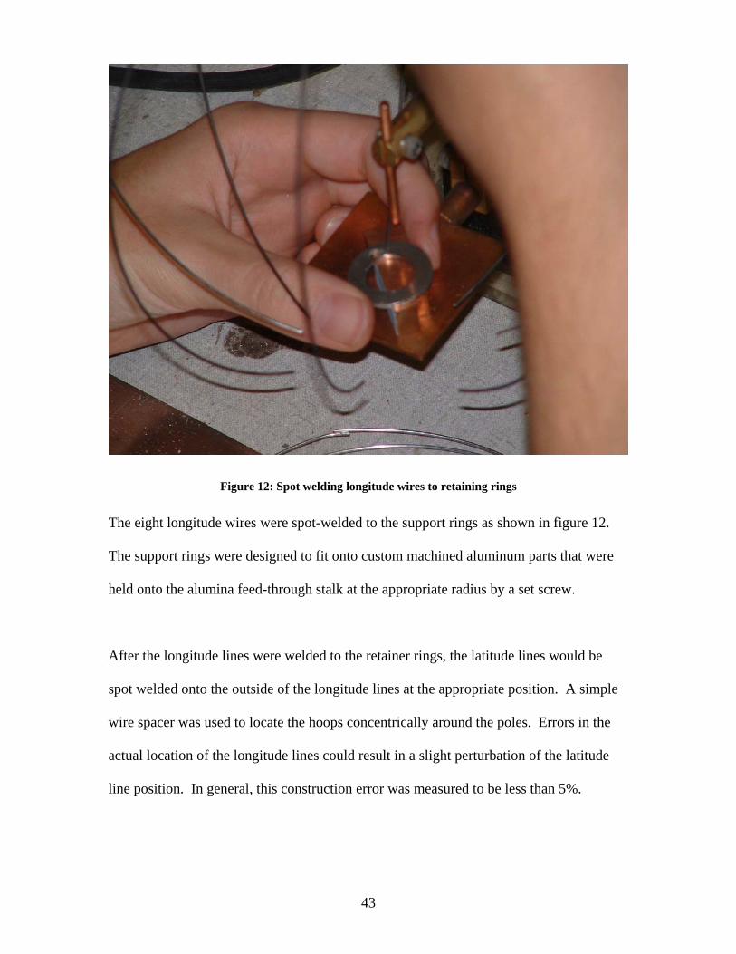
Figure 12: Spot welding longitude wires to retaining rings
The eight longitude wires were spot-welded to the support rings as shown in figure 12.
The support rings were designed to fit onto custom machined aluminum parts that were
held onto the alumina feed-through stalk at the appropriate radius by a set screw.
After the longitude lines were welded to the retainer rings, the latitude lines would be
spot welded onto the outside of the longitude lines at the appropriate position. A simple
wire spacer was used to locate the hoops concentrically around the poles. Errors in the
actual location of the longitude lines could result in a slight perturbation of the latitude
line position. In general, this construction error was measured to be less than 5%.
44
Figure 13: All finished grids
Figure 13 shows all of the completed wire grids. Slight asymmetries in the grid wires are
visible to the naked eye, but position errors of the latitude line locations were all
measured to be less than 8% of the respective radius. Longitude line errors were
significantly less than that.
In order to install the grids in the final multi-grid system, they had to nest one inside the
other. This was accomplished by again cutting the longitude lines near the equator this
time. The cut was made actually just “south” of the equator – right above the southern
“tropic” latitude line. This asymmetric cut was used to improve the ease of re-assembly.
It was desired to have one well-located, stiff wire end, and one more easily manipulated,
45
less well-located wire end that would be moved to align with the stiff end. This was
assumed to be easier than lining up to wire ends of moderate stiffness.
Figure 14: The "Awesome Blossom"
The resulting “half-grids” resemble a flower blossom as shown in figure 14 and a radar
dish or directed listening device as shown in figure 15.
Figure 15: The "radar" with alumina feed-through and aluminum ring supports
46
When the grids are assembled in the chamber, 1” sections of 1/16” diameter stainless
steel tubing are crimped onto the longitude wire ends on the “radar” half, which allow the
insertion and perfect alignment of the longitude lines on the upper, “blossom” half.
Figure 16 shows the completed multi-grid IEC assembly inside the vacuum chamber.
Figure 16: Multi-grid IEC in the vacuum chamber
2.4.3. Ion Source
During the course of these investigations a number of different ion source geometries
were tried. The final ion source used for all of the experiments reported in this thesis
was designed to have a minimal impact on the potential structure inside the anode grid.
47
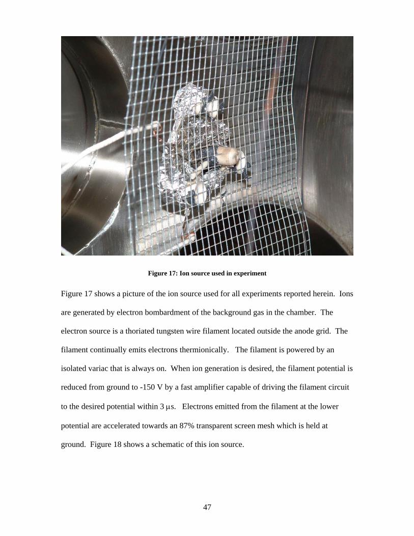
Figure 17: Ion source used in experiment
Figure 17 shows a picture of the ion source used for all experiments reported herein. Ions
are generated by electron bombardment of the background gas in the chamber. The
electron source is a thoriated tungsten wire filament located outside the anode grid. The
filament continually emits electrons thermionically. The filament is powered by an
isolated variac that is always on. When ion generation is desired, the filament potential is
reduced from ground to -150 V by a fast amplifier capable of driving the filament circuit
to the desired potential within 3 µs. Electrons emitted from the filament at the lower
potential are accelerated towards an 87% transparent screen mesh which is held at
ground. Figure 18 shows a schematic of this ion source.
48
The peak of the electron bombardment ionization cross-sections for both Argon and
Helium lie in the range of 100-150eV electron energy. Ions are therefore generated all
around the screen mesh which is positioned such that it is tangent to the surface of the
spherical anode grid. Those ions which are generated inside the anode grid fall into the
well, while those generated outside are accelerated towards the filament and aluminum
foil “neutralizer” which is electrically connected to one of the filament leads.
Figure 18: Schematic representation of ion source
This design results in the quick removal of ions generated outside the anode while
allowing the ions generated inside the anode to fall unobstructed into the IEC potential
well.
49
One drawback of this source is that after the filament potential is returned to ground,
there are ions that were generated between the filament and the screen which now are not
attracted to the neutralizer and are slowly extracted into the IEC potential well by field
penetration through the grid mesh. Due to the high electron density in this region, there
exists a large number of these ions relative to the ions generated on the other side of the
screen. This results in a “slug” of ions at shutdown which can be seen clearly in the data
when the potential structure has good confinement.
2.4.4. Ion Detector
The capacitive probe was the primary ion detector used in these experiments, although
measurements of the current directly to the grid wires were also made at grid potentials
near ground (down to -400V). Figure 19 shows a picture of the capacitive probe wire
poking through the center of the anode mesh.
Figure 19: Wire probe
50
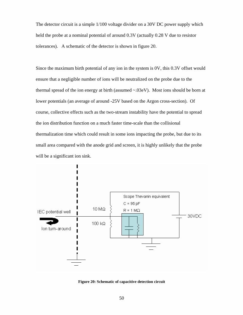
The detector circuit is a simple 1/100 voltage divider on a 30V DC power supply which
held the probe at a nominal potential of around 0.3V (actually 0.28 V due to resistor
tolerances). A schematic of the detector is shown in figure 20.
Since the maximum birth potential of any ion in the system is 0V, this 0.3V offset would
ensure that a negligible number of ions will be neutralized on the probe due to the
thermal spread of the ion energy at birth (assumed ~.03eV). Most ions should be born at
lower potentials (an average of around -25V based on the Argon cross-section). Of
course, collective effects such as the two-stream instability have the potential to spread
the ion distribution function on a much faster time-scale than the collisional
thermalization time which could result in some ions impacting the probe, but due to its
small area compared with the anode grid and screen, it is highly unlikely that the probe
will be a significant ion sink.
Figure 20: Schematic of capacitive detection circuit
51
The Tektronix TDS 2014 scope was attached to the wire probe on the middle of the
divider via a 1X scope probe. With these resistors, the estimated maximum bandwidth of
this detector is around 100kHz which is about at the limit for Argon (with a bounce time
of ~23 µs). Lower value resistors were used to search for the predicted two-stream
instability in Helium due to Helium’s 8 µs bounce time, but lower value resistors reduce
the strength of the signal as well as increase the bandwidth, and Helium had a much
weaker signal to begin with due to its lower ionization cross-section.
The following chapter presents some of the computational modeling that was done prior
to and concurrent with the design and operation of the experiment.
52
3. Computational Modeling for Design
In order to estimate IEC device performance, two independent computer codes were used
to predict ion behavior. The commercial PIC code called OOPIC was introduced in
chapter 1. In addition, a custom code was written in MATLAB to approximate the true,
3-D potential structure. The potential variation along the center of the beamline was then
used in conjunction with the 1-D paraxial ray approximation to solve for the beam
envelope and the maximum confined core ion density. This chapter explains these
computational tools in greater depth.
3.1. Semi-analytic potential model for a multi-grid IEC device
A means of solving for the full, three-dimensional potential structure around a multi-grid
IEC device was desired. Conventional finite difference approaches are not convenient.
The small wire size and the large volume and wire spacing make for a computationally
inefficient solution. Finite element methods with adaptive grid spacing were not
seriously considered due to the scope of the computational problem. Instead, a semi-
analytic approach was adopted with a truncated series potential representation.
3.1.1. Derivation
First the space charge of the trapped ions in neglected, so the potential structure is
assumed to be a solution to the Laplace equation.
02 =Φ∇ Equation 3.1
53
We choose to represent the potential in spherical coordinates where longitude≡θ and
latitude-co ≡φ . The potential and its derivatives can then be represented by a
summation of orthogonal spherical harmonics
[ ]∑ ∑∞
= −=
+− ++=Φ0
)1( cos)(cos),,(k
k
kmi
mk
kikm
kikmi FmPrBrAr θφθφ Equation 3.2
and
[ ]∑ ∑∞
= −=
+−− +−=∂Φ∂
0
)2()1( cos)(cos)1(),,(k
k
km
mk
kikm
kikm
i mPrBkrkArr
θφθφ Equation 3.3
where mkP is the associated Legendre function of the first kind and the index “i” is an
integer from 1 to n+1 where n = # of concentric spherical wire grids. The coefficients A
and B (and the constant offset F) uniquely determine the potential. It can be inferred
from equation 3.2 that for a finite potential solution, all An+1= 0, and similarly, all B1=0.
A finite potential solution also requires 0 and 0 →→ BA as ∞→k . Therefore a
truncated series with sufficiently large “k” should closely approximate the exact solution.
The problem becomes one of solving for the A and B coefficients for the finite series
given the appropriate boundary conditions. With this type of representation, the
boundary conditions become trivial to impose. From continuity we get:
ii FF =+1 Equation 3.4
( ) )12(11 +−− −=− ki
ikm
ikm
ikm
ikm rAABB Equation 3.5
where ri is the radius of the ith grid. We then define an angular delta function such that
αββθβθδθθβθδαα
<<=−≡− ∫∫ 0 ,)()()( ,1)(00 i
i rfdfdr Equation 3.6
Poisson’s equation (the flux condition) at the grid wires can then be expressed as
54
⎥⎦
⎤⎢⎣
⎡−+
+−
−=⎥
⎦
⎤⎢⎣
⎡∂Φ∂
−∂
∂ ∑ ∑= ==
− t
j
l
jii
orr
ii
ljq
tjq
rrΦ
i1 1
1
)2()1
(1 πθδπφδε
Equation 3.7
where qi is the charge per unit length on the grid wires, wireslatitude of # t ≡ , and
wireslongitude of # l ≡ . Note the form of this equation assumes an even angular
distribution of both longitude and latitude lines. From this point forward, the expression
on the right hand side of equation 3.7 will be referred to simply as RHS and the
expression on the left will be referred to as LHS. Substituting r∂Φ∂ on the LHS we get
( ) ( )[ ]∑ ∑∞
= −=
−+−− =−+−−0
1)2(11)-(ki cos)(cos)1(kr
k
k
km
mk
ikm
ikm
ki
ikm
ikm RHSmPBBrkAA θφ Equation 3.8
Then using continuity as expressed in equation 3.5, this expression can be simplified to
( )∑ ∑∞
= −=
− =−+0
11)-(ki cos)(cos1)r(2k
k
k
km
mk
ikm
ikm RHSmPAA θφ Equation 3.9
or
( )∑ ∑∞
= −=
−+ =−+0
12)(k-i cos)(cos1)r(2k-
k
k
km
mk
ikm
ikm RHSmPBB θφ Equation 3.10
It can be clearly seen that the RHS expression uniquely determines the relationship
between the Ai and Ai-1 coefficients, and similarly Bi+1 and Bi coefficients. Because we
know that all the 11 and +nkmkm AB coefficients must be zero in order for the series to
converge at ∞== r and 0r respectively, all of the A and B coefficients can be solved
based upon the RHS expression. These coefficients can be extracted from the
summations because of their respective orthogonality. In particular, cosine orthogonality
can be used to simplify the expression. This step will eliminate the sum over m.
55
∫∫ ′=′ππ
θθθθ2
0
2
0
cos)(cos)( dmRHSdmLHS Equation 3.11
This picks out m=m’ and gives a factor of pi. Similarly, the orthogonality of Legendre
polynomials can be used to eliminate the sum over k. When complete, equation 3.9
becomes
( ) φθθφφππ π
ddmPRHSAAmkmkr m
kikm
ikm
ki ∫ ∫ ′=−
−+ ′′−−
0
2
0
1)1( cossin)(cos)()!()!(2 Equation 3.12
Substituting in the RHS term and integrating reveals the simplified relationship between
the coefficients.
( ) ( ) ⎥⎦
⎤⎢⎣
⎡+
−=−
−+
∫∑=
+−
ππ φφφδπδ
επ
0)(
110
11)-(ki sin)(coscos2
)!()!(r2 dPlP
rqAA
mkmk m
kzlm
t
jtjm
kmio
iikm
ikm
Equation 3.13
where ⎩⎨⎧
≠=
≡ba 0,ba ,1
abδ and z is any positive integer. So to solve for any coefficient,
simply start with 011 ==+km
nkm BA and use.
ikmk
io
iikm A
mkmk
rqA +Χ
+−
=−
)!()!(
21
πε Equation 3.14
1)1( )!(
)!(2
−+− +Χ
+−
= ikmk
io
iikm B
mkmk
rqB
πε Equation 3.15
where ( ) ∫∑ +=Χ=
+
ππ φφφδπδ
0)(
110 sin)(coscos2 dPlP m
kzlm
t
jtjm
km .
56
In this manner the vacuum potential structure around an arbitrary number of
independently charged concentric, spherical wire grids can be modeled in three-
dimensions.
The charge qi on the wires is approximated from a simple spherical capacitive
relationship multiplied by a factor to account for the high transparency of the “spheres”
and the distribution of charge over the surface area (proportional to r2).
( )
⎟⎟⎠
⎞⎜⎜⎝
⎛−
Φ−Φ=
+
+
1
12 11
%4
ii
ii
ioi
rrr
Aq πε Equation 3.16
In the coded implementation of this model, Gaussian distributions of charge in φ and θ
were used instead of delta functions to limit the bandwidth of the spatial representation of
the wires to allow for faster convergence with a smaller truncation value of k. More
information about the details of the modeling can be found in the code contained in the
appendix.
Because a representation of the potential in all three dimensions is difficult to plot,
sample cross-sections are presented in this chapter either at constant r,φ, or θ. In general
a kmax of 32 yielded smooth partial derivatives in r which were required for paraxial ray
beam envelope approximations. Figures 21, 22 and 23 show the modeling results for a
typical potential variation on a plane through the equator.
57
Figure 21: Potential map of equatorial cross-section (φ=π/2) of a multi-grid IEC device.
Figure 22: Different view of same potential map
58
Figure 23: Same potential model, "pie" section from beamline to grid wires
3.1.2. Limitations and Inaccuracies
As with any model, there are limitations to the range of applicability of the model
described in the previous section. In particular, the model has two fundamental
inaccuracies which impose strict limitations on its range of validity:
1) Truncation of the infinite series results in unrealistic high frequency “noise” in
the potential representation – especially when approximating field gradients
over very short distances without applying any type of spatial potential
smoothing near the cut-off frequency.
2) The assumption of constant charge density on the grid wires in wrong. In fact,
the charge density varies significantly from the equator to the poles and in
regions where wires overlap. The proper boundary condition is a constant
potential on the grid wires. Unfortunately, that type of B.C. cannot easily be
59
implemented with this modeling approach. Plots of equipotential surfaces in
figure 24 allow assessment of the significance of this inaccuracy.
Figure 24: Spatial maps of the potential at a constant radius in between latitude and longitude wires
on the equator, note unrealistic high frequency noise in the equipotential representation and
potential deviation at wire overlap at the corners of the figures.
60
Figure 24 illustrates these inaccuracies clearly. An exact model would show no
difference in the potential between the corners and the middle of the wires (along the
edges of the figures). An exact model would also have smooth equipotential surfaces
instead of the ripples introduced by the truncated series approximation.
These inaccuracies, together with the assumptions in the model itself result in the
following limitations:
1) If resolution of the potential and derivatives of the potential are required at a
given spatial frequency, the chosen value of kmax must not only satisfy the
Nyquist condition, it must be twice the typical Nyquist criterion (at least 4
times the frequency) to allow the spatially smoothed signal to satisfy the
Nyquist criterion i.e. the smoothing window should correspond to ½ the size
of the minimum detail desired, and kmax must be ½ the wavelength of the
smoothing window.
2) The potential model should not be used at all within the minimum resolution
(as defined in #1 above) of the grid wire locations.
3) The potential model should not be used within the range of the inaccurate
boundary conditions. This range of inaccuracy can be seen in the
equipotential plots. When the equipotentials do not resemble the bulk shape
of the grid wires (e.g. near the wire overlaps), the model will not give an
accurate potential.
Fortunately, this model is to be used only for the purposes of preliminary experiment
design, and for that reason, the only potential that is of significance is that along the
61
center of the beam line. This model should yield reasonable estimates of the potential for
these crude purposes.
Figure 25: Constant θ cross section plots of potential structure of a multi-grid IEC device on a grid
wire v. on the beam path
Figure 25 illustrates the continuous potential (upper plot) and derivative of the potential
(lower plot) along the beam line and the discontinuous derivative of the potential at the
grid wire locations as a result of the charge located there. The upper plot also shows the
62
regions where the potential structure is “confining” to ions and where it is “unconfining”
i.e. near the lowest potential grid.
3.2. 1-D Paraxial Ray Equation Approximation
In order to estimate the maximum confined non-neutral ion density achievable in a multi-
grid IEC device, a simple model of the variation of the radius of an ion beam based on
the paraxial ray equation was developed.
3.2.1. Model Description
The output from the semi-analytic potential model described in section 2.1 was used to
approximate the potential and the derivatives of the potential along an equatorial beam
path in the multi-grid IEC device. The paraxial ray equation was used to predict the
evolution of the ion beam envelope based upon that variation in the axial potential. This
model was derived primarily from the work of Humphries [362]. Since there are no
magnetic fields in an IEC device, the general form of the paraxial ray equation reduces to
RK
RRRR ++
ΦΦ
−Φ
Φ−= 3
2
4''
2'''' ε
Equation 3.17
where R is the radius of the beam envelope (perpendicular to the beam line and the r
vector in the IEC device). ε in this equation is the beam emittance, and K is the
generalized perveance defined relativistically as
( )32 cmeIK
oo
o
βγπε= Equation 3.18
63
In this equation, 2
21
1
cv−
=γ , c is the speed of light and β=v/c the ratio of the ion
velocity to the velocity of light. The generalized perveance is proportional to the number
density of ions, and it is the term that accounts for the space charge of the beam in this
simple model. Although it is inaccurate, zero emittance (the laminar beam
approximation) is assumed because the goal of this model is to predict the maximum
space-charge limited confined ion density in the core of the device, not to predict a
particular beam envelope.
3.2.2. Numerical Integration of Beam Envelope
Symmetry of the ion beam in the core of the device (a zero slope condition) is assumed
along with a core radius. These assumptions provide the initial boundary conditions from
which the paraxial ray equation can be integrated. MATLAB’s “ode45” routine is then
used to integrate the paraxial ray equation from the core out to the radius of the injector.
In order to verify convergence of the integration, the numerical integration is repeated in
reverse, this time the initial conditions are the final conditions of the 1st integration and
the beam envelope is integrated on the way in. The deviation of the final radius and slope
of the beam envelope is compared to the assumed initial radius to verify convergence of
the routine.
Figure 26 shows an example of a beam envelop that did not converge, while figure 27
shows a converged beam envelope.
64
Figure 26: Improperly converged integration example
3.2.3. Iterative Solution to Maximum Beam Density
A maximum acceptance window which defines how close the modeled beam is allowed
to come to the grid wires is assumed (typically 70-90% of the height of the grid wire
from the beam axis). The initial beam current (ion density) is assumed to be two orders
of magnitude lower than the density at which space charge effects are expected to be seen
based on PIC modeling and simple back-of-the-envelope Child-Langmuir calculations for
this size device. The beam envelop is then solved out to the injector radius. Near the
injector radius the paraxial ray equation loses all validity because the implicit
linearization assumes beam-like behavior which is not the case near the ion injection
potential. If the beam envelope does not exceed the acceptance window at the grid-wire
locations, the core density is increased by a factor of two, and the integration is repeated.
65
This iterative process is repeated until the space charge effects of the beam force the
beam envelope outside the acceptance window of one of the grids at which point the
routine is stopped. The maximum confinable ion density is thereby found to within a
factor of two.
Figure 27: Potential map (top) and beam envelope (bottom) versus beam-line position for very small core focus and high core ion density (not reproducible in OOPIC)
Given the assumptions implicit in this method, it was expected to yield results only
accurate to within an order of magnitude of the actual space charge limit, and when
exceedingly small core radii were assumed, the maximum predicted density differed from
the PIC model by more than an order of magnitude. When the assumed core radius was a
significant percentage of the innermost grid radius, comparison to OOPIC modeling
revealed agreement to within a factor of 2. Figures 28 and 29 show the similarities in
the predicted beam envelopes from the modeling described above and the OOPIC
66
simulation. It is worth noting that OOPIC has only a 2-dimensional model of the
potential, so minor deviations between the two codes should be expected.
Figure 28: Model with large assumed core size that matches OOPIC results to within a factor of 2
Figure 29: OOPIC model showing similar beam envelope for similar grid voltages and ion mass
67
3.3. Simulated Annealing IEC Design
Due to the large number of independent variables involved in the design of a multi-grid
IEC experiment, a code was developed based upon the beam modeling in the prior
section to help find an optimal or near optimal design for a multi-grid IEC reactor given
the limited resources of our group. Simulated Annealing (SA) is a design methodology
for complex systems which depend on multiple independent design variables. SA is an
active area of research in complex systems, and it has been shown to be an effective
optimization tool for the design of complicated systems. Because of the large number
of independent design variables (grid positions and potentials) in a multi-grid IEC,
simulated annealing design was explored.
The premise of simulated annealing design is that while there can be a very large number
of independent design variables, the quality of any design can be quantified by a singular
metric known as an energy function. The lower the energy function, the better the
design. Because the overall design space can be very complex, there can be many local
minima which could fool a gradient-search based design code. An SA approach initially
resembles a Monte-Carlo method in that design variables are changed at random and
even if a given change results in a higher value of the energy function, at the beginning
that change is kept and another change to the design is made. The best design found is
always kept in memory. As the code progresses, the bounds of whether a new design
change is kept are gradually reduced until the code simulates a traditional gradient search
method. This approach which gradually transforms itself from a Monte-Carlo design tool
to a gradient search method has been shown to be quite good at finding designs at or near
the global minimum energy function. The gradual decrease in the accepted bounds of
68
energy resembles the physical process of cooling (hence “simulated annealing”) – if it is
done sufficiently slowly, the global minimum energy (single crystal) state will emerge.
3.3.1. Energy Function
For the multi-grid IEC design problem, an energy function was desired which would give
a design with the maximum fusion energy output given the constraints on the design
variables. The energy function was therefore set as proportional to the inverse of the
estimated fusion power output from the device.
( ) 322
1
corecoreinjcore RntionEnergyFunc
Φ−Φ= Equation 3.19
The fusion reaction rate is proportional to the square of the ion density in the core and the
cube of the core size. The key implicit assumption here is that the fusion cross section is
proportional to the square of the core ion energy, this assumption is only valid up to a
certain fraction of the energy of the maximum fusion cross section for a given reaction
(~50keV for deuterium). Since the grids in our experiment are limited to -10kV
potentials by the power supplies available, this assumption should be good for the current
application. If future experiments are to use the same code, an energy function which
incorporates the actual variation of the fusion cross-section for the desired fuel would be
better.
3.3.2. Design Variables and Limitations
The radius and potential of each grid are all independent design variables. In addition,
the radial location of the injector could be moved. The anode radius and the number of
latitude and longitude wires were fixed, and the core radius was assumed to be a constant
69
fraction of the innermost grid radius. The innermost grid radius was limited to 10 cm
maximum, and the grids were not allowed to be positioned within 2 cm radially of one
another. These constraints were imposed for ease of fabrication, diagnostic access, and
assembly.
3.3.3. Summary of SA Results
The simulated annealing design code converged on an optimal solution after 1600
independent and random design perturbations.
Figure 30: Final Convergence History for Simulated Annealing Design
The initial design guess had an energy function that was nearly an order of magnitude
higher than the final solution. Figure 30 shows the progression of the design with each
successive iterative perturbation. The code successfully resulted in a grid design and a
70
recommended potential structure that would result in a significantly higher fusion power
output than the initial guess.
Figure 31: Number of occurrences v. energy in final SA run
The progression of the “cooling” of the design can be viewed either by plotting the
energy v. the iteration number, or by looking at the number of occurrences at different
energy levels and the average energy level for all iterations at a particular pseudo-
temperature as shown in figure 31.
The “freezing” of the design can be seen by the drop in the “entropy” and the rapid rise in
the “specific heat” of the design as illustrated in figure 32.
71
Figure 32: Evolution of the SA design showing the freezing of the configuration
72
The final output of the SA code gave the potential structure and beam envelope shown in
figure 33.
Figure 33: Final Output of SA design showing largest allowed inner grid and bunching of
accelerating grids at coded limit of 2 cm.
As can be seen in figure 33 above, the SA design code pushed the inner-most grid out to
the coded limit of 10 cm. It also bunched the inner grid and the two accelerating grids to
the minimum coded spacing limit of 2 cm. These can be explained by simply
maximizing the size of the fusing volume and minimizing the spacing between the
accelerating grids to reduce the space charge effects by maximizing the local field
curvature near the accelerating grids. The injector potential is very close to ground, and
the core potential is very close to the minimum of -10kV. In fact the second and third
grids out from the center are at -10kV and 0V respectively – the maximum possible
potential difference and the minimum spacing. It is interesting to note that neither the
73
first grid nor the fourth grid have any significant role to play in shaping the potential
structure. This suggests that the optimum number of grids may be 3 (not 5). It is
interesting to note that the while the energy function did change substantially, little of
that change was due to a difference in density. In fact, the energy function showed the
most sensitivity to the size of the innermost grid (and hence the assumed core size) and
the difference between the core potential and the injection potential. The maximum
density for Argon ions in the system was always seen to be around 8e13 m-3.
While this tool may be useful for future investigations of actual fusion reactors, it was
less useful than anticipated for informing the design of the present experiment. This was
partly due to relating the energy function to possible fusion output instead of relating it to
a measurement of the confinement experiment. Because most of the signals in the
experiment will be proportional to the number of trapped ions, and that number does not
seem to vary substantially given the maximum potential difference and fixed dimensions
desired for experimental access, the actual hardware design was based off of
experimental convenience instead of the results of this analysis. The code is included in
the appendix of this thesis for future reference.
3.4. Modeling with commercial OOPIC Pro code
Throughout these investigations, extensive use of the OOPIC Pro code was made in order
to gain insight into the detailed physics of the multi-grid IEC device. OOPIC Pro is a 2D
planar particle in cell model with Monte Carlo collisions [358]. This section details some
74
of the predictions that were made prior to experiment operation based upon this useful
tool.
3.4.1. 2-Grid Modeling and Confinement Estimations
Initial computational investigations explored the conventional, 2-grid IEC configuration.
As illustrated in the first chapter, at the pressures which yield the highest neutron rates in
the literature (4.0 microns) [18], the mean free path of ions in the system is less than the
typical device diameter. The majority of these reactions were shown to be beam-
background reactions [357]. As the pressure is reduced, the reaction rate peaks at
approximately 0.1 microns and then is also reduced, but the ion confinement time is
increased. In the limit of a perfect vacuum, the only means of ion loss from the IEC
system are:
1) Ion neutralization on a grid wire via unconfined/chaotic trajectory or ion-ion
collisional scattering
2) Ion neutralization on the anode via ion-ion collisional energy spread
3) Fusion
Hirsch estimated the average number of passes through the center of a 2-grid device in
this hard vacuum regime with a simple grid transparency argument [21].
21 ννδ−
= Equation 3.20
In this simple model, ν is the grid transparency (typically 0.9 to 0.98) and δ is the
expected number of passes through the center of the device. The sole loss mechanism
implicit in this model is number 1) in previous list, i.e. loss to the grid wires.
75
OOPIC was used to check the validity of this assumption. A simple 2-grid model was
developed which did not contain any of the realistic field asymmetries which had already
been shown to be capable of reducing the ion confinement time to 1-5 passes. Due to the
finite grid size the grid wires are larger than they typically are experimentally which
limits the modeled transparency. In this model the grid transparency is 88% which
should yield 4 passes through the center on average according to the Hirsch model. The
OOPIC model presented here assumes that the ions are Ar+1 and the cathode potential is -
7500 V resulting in an ion bounce time of approximately 8 µs or a single pass time of 4
µs. The average confinement time is therefore expected to be 16 µs.
Figure 34: Low pressure, 2-grid OOPIC simulation, ion injector on
Figure 34 shows a 2-grid OOPIC model with no electric field asymmetries and no neutral
background gas. When the simulated ion injector is turned off, the number of ions in the
system will decrease as ions are lost. The 1/e time of the decay curve can be compared to
the expected confinement time based on the Hirsch formula.
76
Figure 35: Time evolution of Argon +1 ions in the simplest 2-grid OOPIC model (no background gas)
Figure 35 shows the time evolution of ions in this model under these idealized conditions.
Not surprisingly, when injection is turned off at 200 µs (top two images is figure 35),
there is a rapid loss of ions on the order of the Hirsch confinement time. The top two
77
images in figure 35 show the spatial location of the ions on the left and the spatial density
of the ions on the right. The rapid loss of ions appears to be localized in space – it is
only the ions outside of what may be considered a “grid acceptance window” which are
lost on this rapid 16 µs timescale.
The middle two images in figure 35 show the ions in the system 230 µs after termination
of injection. The image on the right is the same spatial representation of the location of
the ions, while the image on the left shows the time history of the total number of ions in
the system. It is clear that the rate of decay of ions in the trap has changed in such a way
that it is no longer proportional to the number of ions in the trap as would be expected if
confinement were either limited by statistical grid wire interception or collisions with
background gas. In fact, the 1/e decay time of those ions inside the grid acceptance
window is approximately 40ms -- orders of magnitude longer than the 16 µs predicted
from the transparency model. Even though the local field around the cathode is
nominally defocusing, the overall ion confinement is good enough in this idealized
simulation that the two-stream instability has time to develop and bunch the ions as seen
in the bottom two images of the figure 35 at a time of approximately 1ms after
termination of injection. This bunching was first identified by McGuire [357] in
computational modeling of IEC devices and is a saturated mode of the well-known
streaming instability in this type of device.
When asymmetries in the field structure are modeled by introducing the realistic effects
of a stalk or feed-through, however, the Hirsch model does much better at predicting ion
confinement in a 2-grid IEC device.
78
Figure 36: 2-Grid OOPIC model showing ions impacting cathode after 1/2 to 5 passes
Figure 36 shows how the field asymmetries caused by the cathode feed stalk result in
very short ion lifetimes of 1-5 passes through the inner cathode grid -- dependent upon
the location of the ion injector(s).
These simple simulations suggest that the “transparency” model developed by Hirsch
may not be a good means of estimating the confinement time in a 2-grid IEC device if the
device is carefully constructed to minimize the effects of asymmetric background fields,
but it should be reasonable for most 2-grid devices with realistic field asymmetries due to
feed through stalks.
3.4.2. Multi-Grid Modeling and Confinement Estimations
One very effective way of shielding the effects of feed-through asymmetry and
improving ion confinement is by carefully tailoring the field structure with multiple
independently biased grids. The efficacy of this approach was clearly illustrated using
79
OOPIC in chapter 1 figures 3 and 4. McGuire has conducted extensive investigations
into this technique using OOPIC [357]. His original code was used as the basis for all
OOPIC modeling of multi-grid IEC devices contained in this thesis.
If we assume that the multiple grid configurations are capable achieving the highly
confined ion trajectories observed in the simulations, the primary limiter on ion
confinement is scattering due to collisions. Scattering with background gas and other
ions and thermalization become the primary loss mechanisms. Therefore it should
become possible in UHV conditions to push the theoretical limits proposed by Rider
[175].
In order to achieve these theoretical improvements, an experiment was designed with the
goal of demonstrating the potential to significantly improve confinement time using
multiple grids. This experiment is operated under high vacuum conditions; lower than
the pressures at which most IEC experiments are run, but above the UHV pressures that
would be required to push the limits of thermalization. At these pressures, collisions with
the background gas are the biggest limiter to confinement. OOPIC was used to estimate
the effects of background gas on ion confinement times in the multi-grid experiments.
Figure 37 shows a typical, multi-grid simulation geometry in OOPIC.
80
Figure 37: Typical simulated multi-grid geometry, x and y dimensions are meters, grid locations and ion injector geometry are based upon the physical experiment
In order to facilitate evaluation of the 1/e time, the ion signal is normalized to the level at
the time when the injection is turned off. This practice will be used throughout the thesis.
The complete, un-normalized curves typically resemble the curve shown in figure 38:
Figure 38: Typical plot of number of macroparticles in an OOPIC simulation
81
The standard practice that was adopted for both computational experiment and physical
experiment was to inject ions for 1ms then turn off the injector and observe only the
decay portion of the curve. While the maximum number of ions in the system (and hence
the signal strength) can vary with the strength of the source, the decay curve will only be
a function of the sink. Comparing the 1/e times of the normalized decay curves will
therefore give the best indication of actual confinement time of ions in the device.
Figure 39 shows a map of the potential structure in a typical multi-grid OOPIC
simulation which illustrates the ability of the multiple grids to “shield out” the effects of
the feed-through stalks.
Figure 39: OOPIC multi-grid potential model for a scenario with good ion confinement
Not all multi-grid scenarios showed improved confinement. In fact the ion confinement
was expected to be quite sensitive to the particular grid potentials based upon OOPIC
modeling.
82
Figure 40: Symmetric multi-grid field with poorly confined ions
In the figure 40 above, the field structure is symmetrical, but the ions are not well
confined due to a field structure that prematurely focuses the ion beam. The beam then
freely expands in the core region where there is little confining field curvature. On the
opposite side of the device, the over-focused field again skews the trajectory of the beam
which results in a wider beam envelope. Ions are quickly lost to the grid wires, and the
overall confinement is very poor. It is clear from this one example that the specific
potential structure imposed by the grids can be quite important in determining the ion
confinement time even in the absence of field asymmetries.
When a small asymmetry in one of the grid wires is introduced (a one grid space
perturbation which corresponds to a 2.5% change in position of one grid wire), the poor
confinement is even more pronounced. Figure 41 shows the effect of an unperturbed
(left) and perturbed (right) wire in the multi-grid simulation. The perturbation introduces
field asymmetries which tend to skew the ion beam
83
Figure 41: Comparison of perfectly symmetric field (left) with a 2.5% location perturbation on one wire (right). The perturbed wire is the second grid from the center in the upper left hand quandrant.
If the imposed potential structure results in a well confined ion beam (figure 42),
however, there is much less sensitivity in the overall shape of the beam envelope to
geometric perturbation in either the grid wires or the ion source.
Figure 42: Good multi-grid confinement with unperturbed grids and concentrated ion source (left), and highly perturbed grids (5% on 2nd grid and 2.5% on 3rd grid) with diffuse ion source (right), same grid potentials
The geometry on the right hand side of figure 42 above is representative of the worst case
scenario for the experiment as designed at an achievable pressure of 8e-5 torr. For this
model with Helium gas, He+1 ions and a cathode potential of -5000 V, the predicted 1/e
confinement time is 8 µs or approximately 2 passes as shown in figure 43.
84
Figure 43: Normalized plot of the decay of the number of ions in the "worst case" OOPIC simulation for 8e-5 mbar He.
Once the experiment was completed and data with various diagnostics was taken, it
became clear that for Helium, the pressure range with the highest S/N was 1e-4 mbar or
8e-5 torr. A comparison of best expected confinement time at this pressure was then
conducted to evaluate how close to the best simulated confinement we had achieved in
the actual experiment. The worst case scenario is presented in figure 43 above.
Although the worst case 1/e confinement time of 8µs is quite bad, it is still better than the
perfect vacuum 2-grid simulation (5.4 µs) with the stalk assymmetry.
The decay for the best case scenario (left side of figure 42) is shown in figure 44 below.
The grid potentials from anode to cathode for both of these runs are [0, 0, -1000, -1500, -
5000]. It is worth noting that the geometry of the ion source combined with large
85
(though not unreasonable) asymmetries in the grid wires have the potential to alter the 1/e
confinement time of the system by a factor of 5. This change is purely geometrical as a
result of the induced field asymmetries, i.e. the pressure, the gas, and the grid potentials
are all the same in these two scenarios.
Figure 44: Normalized decay curve of best case, Helium at 8e-5 torr
These results can also be compared with estimations of the mean free path for collision
and charge exchange at this mean ion energy and device pressure.
σσλ
PkT
nmfp ==1
Equation 3.21
Assuming a room temperature background gas at 1e-4 mbar, the mean free path for
charge exchange at this pressure and average energy is only 4.1 m corresponding to 8
passes or 32 µs based on the charge exchange cross-sections given by Hegerberg [352].
86
The OOPIC simulation in conjunction with these simple calculations suggests that the
dominant loss of ions at this pressure is due to charge exchange collisions with the
background gas. While all charge exchange reactions will result in some loss of energy
(via the fast neutral), not all charge exchange reactions result in direct loss of an ion from
the system (especially those ions that undergo charge exchange near the edge of the
potential well), it is therefore possible that confinement times longer than the mean time
until charge exchange could be expected.
The effects of changing the background gas pressure were simulated. For all of these
multi-grid runs, the same confining potentials were applied to the grids [0, 0, -1000, -
1500, -5000] volts, and the corresponding grid radii are [.25, .17, .10, .075, .05] meters.
As expected, the 1/e confinement time is proportional to 1/p for multi-grid experiments.
1/e confinement time for 2-grid experiments shows a general insensitivity to pressure in
the regimes explored. Figure 45 clearly shows the expected difference between 2-grid
and multi-grid confinement times based on OOPIC modeling.
Figure 86: Normalized oscillation envelope and exponential-sigmoid curve fit for the test plotted in figure 85 (Argon, 1.9e-6 mbar)
If we attempt to extrapolate the 1/e confinement time from figure 85 based on the
amplitude of the oscillation envelope in the signal (figure 86), it can be seen in that the
1/e time is approximately 400 or 33 passes. It is interesting to note that if the trend in
figure 74 were to be extrapolated to this low pressure, the predicted confinement time
would be 875 µs, so it is clear that the actual confinement time does not follow that linear
extrapolation under these circumstances. It may be that the presence of the instability
causes a more rapid loss of ions than would otherwise be expected.
131
The curve fit shown in figure 86 is a decaying exponential multiplied by a sigmoid
function. The decaying exponential represents the continuous loss of ions from the
system at a rate proportional to the number of ions in the system. The sigmoid function is
used to represent the growth and saturation of the streaming instability which causes
bunching that increases the amplitude of the detected ion signal. The specific function
that is normalized and plotted in figure 85 is
( )⎟⎠⎞
⎜⎝⎛ ⎟
⎠⎞⎜
⎝⎛ −−+
−=
00006.0)0001.0(exp1
0004.0exp)(
t
ttEnvelope Equation 4.5
Note the 100 µs time shift of the sigmoid to align the growth with the time axis of the
data. Based on this model, the growth and saturation of the instability happens on a much
faster time scale (60 µs) than the loss of ions from the system (400 µs). The growth of
the instability in these data may be artificially accelerated, however, by the injection of
the ion slug (an artificially large perturbation) at ion-source shut-off.
Due to this different method of evaluation of confinement time in the presence of the
instability at these lower pressures, these confinement time data are not included in the
earlier presentations of confinement time data. There is also no good measurement of the
two grid confinement time at this lowest pressure for purposes of comparison. If the
trend at the lowest pressures is extrapolated from figure 59, the 2-grid confinement would
be approximately 135µs at this pressure – a factor of 3 lower than the measured 400µs
multi-grid time.
132
The specific conditions and mechanism for this instability are investigated in depth in the
Ph.D. thesis of Tom McGuire. Experimentally, in the grid geometry tested, the instability
was seen with a number of different confining potential structures. The best signal (most
bunching) at all pressures was achieved with grids at the following potentials: [-5000, -
2400, -830, -14, 0]. Double bunching was never seen in experiment although McGuire
sees it in computational modeling. The detailed investigation of this phenomenon is
beyond the scope of this work.
133
5. Conclusions and Future Work
Computational and experimental investigations into improving ion confinement in
inertial electrostatic confinement systems were conducted. The baseline 2-grid system
was compared to a multi-grid system and it was found that the shaping of the electrostatic
background field could improve ion confinement in the high vacuum operating regime.
The PIC predicted ion bunching mode which is believed to be a saturated two-stream
instability was also seen for the first time in an IEC experiment. Computational
predictions of 2-grid confinement using OOPIC were quite poor, but modeling of the
pressure sensitivity of multi-grid confinement was matched quite well in experiment
down to pressures at which the two-stream instability was seen to develop. At these
pressures (below ~4e-5 mbar), the 1/e confinement was difficult to clearly distill from the
data using the same techniques due to the presence of the instability. An envelope
amplitude technique was used to show that a multi-grid Argon ion confinement test at
1.9e-6 mbar had a 1/e confinement time of approximately 400µs, or approximately 33
passes compared to the two grid baseline in which the 1/e confinement time was shown
to be approximately 10 passes at best.
5.1. Contributions of this thesis
This thesis reports on the modeling, design, construction, and testing of the first
published multi-grid IEC ion confinement experiment. The general scaling for non-
neutral IEC systems was derived. A useful non-dimensional number for non-neutral IEC
systems was proposed. The design and construction of the first multi-grid IEC
experiment was reported. A 3-dimensional, multi-grid semi-analytic potential model was
134
described. The first direct measurements of ion confinement times in a multi-grid IEC
device were reported. Computational experiments of particle-in-cell models created in
OOPIC were compared to measurements of a physical experiment, and the potential for
multi-grid IEC devices to improve ion confinement times was shown both
computationally and in experiment. Detection of the computationally predicted two-
stream instability at the ion bounce frequency was also reported.
5.2. Suggestions
The current experimental hardware could be used to further these investigations into the
confinement properties of multi-grid IEC systems at HV and UHV pressures more
effectively if an improved ion source with a much higher pressure in the ionization region
than in the rest of the chamber is developed. This type of source could decouple the ion
signal strength from the background density which could allow for much more accurate
measurements at much lower pressures. It is also desirable to redesign the ion source to
eliminate the slug of ions that is injected when the source is shut down.
It would be interesting to experimentally explore the conditions for the onset of the
instability. This type of investigation would be greatly informed by continued theoretical
research such as is embodied in the work of McGuire [357].
Because of the scaling of this type of non-neutral IEC device, improved power outputs
could be achieved by shrinking the size of the device. The limits to this shrinkage would
be imposed by surface flashover considerations, or possibly by cold Fowler-Norheim
135
emission of electrons from the cathode resulting in rapid loss of efficiency at very small
scale. Such analysis is left to future students.
136
Appendix: Code This appendix contains some of critical pieces of code that were generated in order to
produce the computational results reported in this thesis. Code is written for MATLAB
Version 14 and OOPIC Pro Version 1.0. For compactness of this document, only one
version of the OOPIC model is included (GridDiagnostics5.inp).
137
Matlab Code For reference I have only included the MATLAB code which was directly used in the Simulated Annealing design routine. Elements of this code are used in other scripts to plot parameters of interest, but the included package is self-sufficient for the SA design process.
Annealit2thengrad.m % Simulated Annealing design script for IEC fusion experiment % Carl Dietrich 5/31/05 % It is assumed that there are 8 longitude lines and 4 latitude lines of % even spacing (45 and 36 degree separations), and that the 5th, outermost grid is % grounded at a radius of 0.25 m. % Configuration = [Ro Rinjector Rgrid1 Rgrid2 Rgrid3 Rgrid4 Potgrid1 Potgrid2 % Potgrid3 Potgrid4]; clear all close all Ro = .01; Rinjector = .18; Rgrid1 = .05; Rgrid2 = .07; Rgrid3 = .1; Rgrid4 = .14; Potgrid1 = -7000; Potgrid2 = -10000; Potgrid3 = -4000; Potgrid4 = -1000; Configuration = [Ro Rinjector Rgrid1 Rgrid2 Rgrid3 Rgrid4 Potgrid1 Potgrid2 Potgrid3 Potgrid4]; %[xbest,Ebest,xhist]=SA(xo,file_eval,file_perturb,options); % options algorithm option flags. Uses defaults, [ ], if left blank % (1) To - initial system temperature - automatically determined if % left blank ([]). To should be set such that the expression % exp(-E(xo)/To)>0.99 is true, i.e. the initial system is "melted" % (2) Cooling Schedule: linear=1, exponential=[2] % (3) dT Temp. increment, e.g. [dT=0.9] for exp. cooling Tk=dT^k*To, % abs. temperature increment for linear cooling (Tk+1=Tk-dT); % (4) neq = equilibrium condition, e.g. number of rearrangements
138
% attempted to reach equilibrium at a given temperature, neq=[5] % (5) frozen condition - sets up SA exit criterion % nfrozen = non-integer, e.g. 0.1 SA interprets this numbers as Tmin, % the minimum temperature below which the system is frozen. % nfrozen = integer ,e.g. 1,2.. SA interprets this as # of successive % temperatures for which the number of desired acceptances defined % under options(4) is not achieved, default: nfrozen=[3] % (6) set to 1 to display diagnostic messages (=[1]) % (7) set to 1 to plot progress during annealing (=[0]) To=1e2; options(1)=To; schedule=2; options(2)=schedule; dT=.1; options(3)=dT; neq=100; options(4)=neq; nfrozen=0.001; options(5)=nfrozen; diagnostics=1; options(6)=diagnostics; plotflag=1; options(7)=plotflag; rand('state',sum(100*clock)); tic [BestConfig,Ebest,xhist]=SAmodCarl(Configuration,'griddesigneval2','PerturbConfig2',options) toc [a b]=size(BestConfig); PlotConfig2(BestConfig(a,:)); title('Modified SA Results'); coreacceptance = .5; mingap = .02; LB(1)=0; UB(1)=BestConfig(a,3)*sin(pi/8)*coreacceptance; %max Ro is the first grid radius times the acceptance LB(2)=BestConfig(a,5); % lower bound of Rinj is 3rd grid radius UB(2)=.25; LB(3)=BestConfig(a,3); %1.5*mingap; UB(3)=(BestConfig(a,4)+BestConfig(a,3))/2 - mingap/2; LB(4)=UB(3)+mingap; UB(4)=(BestConfig(a,5)+BestConfig(a,4))/2 - mingap/2; LB(5)=UB(4)+mingap; UB(5)=(BestConfig(a,6)+BestConfig(a,5))/2 - mingap/2; LB(6)=UB(3)+mingap; UB(6)=.25-mingap; LB(7)=-10000; UB(7)=0; LB(8)=-10000; UB(8)=0; LB(9)=-10000;
139
UB(9)=0; LB(10)=-10000; UB(10)=0; tic [NewBestConfig,LowestEnergy] = fmincon('griddesigneval2',BestConfig(a,:),[],[],[],[],LB,UB) toc PlotConfig2(NewBestConfig); title('FMINCON Gradient Search Results'); % Save results to file: dumpfilename = strcat('SA_FMINCON_',datestr(now,'mmm-dd-HHMM')); fid=fopen(dumpfilename,'w'); if fid==-1 error = 'Unable to open dump file!' end fid=fopen('filename','w') fprintf(fid,'%s \n',num2str(NewBestConfig)); fclose(fid);
140
Griddesigneval2.m % Energy evaluation function for simulated annealing design of multi-grid % IEC fusion reactor experiment % Carl Dietrich 5/29/05 % Input is an array % Configuration = [Ro Rinjector Rgrid1 Rgrid2 Rgrid3 Rgrid4 Potgrid1 Potgrid2 % Potgrid3 Potgrid4]; % It is assumed that there are 8 longitude lines and 4 latitude lines of % even spacing (45 degree separations), and that the 5th, outermost grid is % grounded at a radius of 0.2 m. function Energy = griddesigneval(Configuration) global rx pot_beam pot_prime_beam pot_dubprime_beam K inj_pot e=1.602e-19; epso=8.854e-12; c=3e8; % Input the desired grid structure: r = [Configuration(3) Configuration(4) Configuration(5) Configuration(6) .25]; % grid radius vector if r(1)>r(2) | r(2)>r(3) | r(3)>r(4) | r(4)>r(5) disp('Warning: Invalid grid configuration!') r = r Energy = 10000 return end Voltagedesired = [Configuration(7) Configuration(8) Configuration(9) Configuration(10) 0]; n=max(size(Voltagedesired)); solidityfudgefactor = 2.75e-5; for i=1:n-1 deltaV(n-i) = -(Voltagedesired(n+1-i)-Voltagedesired(n-i)); Qins(n-i) = solidityfudgefactor*4*pi*epso*deltaV(n-i)/(1/r(n-i)-1/r(n+1-i)); end Qins(n)=Qins(n-1); Qdesired(1)=Qins(1); for i=2:n Qdesired(i) = Qins(i)-Qins(i-1); end q = Qdesired./r.^2;%[10.5e-8 -2.1e-7 7.5e-8 0]; % grid charge vector t = 4; % number of latitude wires l = 8; % number of longitude wires thickness =.001;% wire thickness kmax = 32; mult = kmax/(2*l);
141
% Calculate coefficients: %tic [Abar, Bbar]=solve_coeff(r,q,t,l,thickness,mult); %toc %tic phi = pi/2; theta = 0; %pi/l; divs = 300; dr = max(r)/divs; rx=[0:dr:max(r)]; for i=1:(divs+1) if rx(i)<.01 pot(i) = spherical_potential_norm_posm_bar(r,Abar,Bbar,.01,theta,phi); else pot(i) = spherical_potential_norm_posm_bar(r,Abar,Bbar,rx(i),theta,phi); end end edge_ground = -pot(divs+1); pot = pot+edge_ground; for i=1:(divs+1) if i==1 pot_prime_wire(i)=0; elseif i==divs+1 pot_prime_wire(i)=(pot(i)-pot(i-1))/dr; else pot_prime_wire(i)=((pot(i)-pot(i-1))/dr+(pot(i+1)-pot(i))/dr)/2; end end theta = pi/l; for i=1:(divs+1) if rx(i)<.01 pot_beam(i) = spherical_potential_norm_posm_bar(r,Abar,Bbar,.01,theta,phi); else pot_beam(i) = spherical_potential_norm_posm_bar(r,Abar,Bbar,rx(i),theta,phi); end end pot_beam = pot_beam+edge_ground; for i=1:(divs+1) if i==1 pot_prime_beam(i)=0; elseif i==divs+1 pot_prime_beam(i)=(pot_beam(i)-pot_beam(i-1))/dr; else
142
pot_prime_beam(i)=((pot_beam(i)-pot_beam(i-1))/dr+(pot_beam(i+1)-pot_beam(i))/dr)/2; end end for i=1:(divs+1) if i==1 pot_dubprime_beam(i) = 0; elseif i==divs+1 pot_dubprime_beam(i)=(pot_prime_beam(i)-pot_prime_beam(i-1))/dr; else pot_dubprime_beam(i)=((pot_prime_beam(i)-pot_prime_beam(i-1))/dr+(pot_prime_beam(i+1)-pot_prime_beam(i))/dr)/2; end end %%%%%%%%%%%%%%%%%%%%%%%%%%%%%%% K=zeros(size(rx)); % Initial beam envelope conditions Ro=Configuration(1); r_inj = Configuration(2); mi = 40*1.67e-27; % Argon inj_pot = spherical_potential_norm_posm_bar(r,Abar,Bbar,r_inj,pi/l,pi/2)+edge_ground; inj_pot_dtheta = spherical_potential_norm_posm_bar(r,Abar,Bbar,r_inj,2*pi/l,pi/2)+edge_ground; dphidtheta=(inj_pot_dtheta-inj_pot)/(pi/l); if dphidtheta<0 disp('Reflection region is defocussing => bad design') Energy = 10000 return end vtherm=340; Rprimeo=0; Rfinal = 0; Rprimefinal = 0; no=2e13; YO = [Ro Rprimeo]; OPTIONS = ODESET('RelTol',1e-4,'AbsTol',1e-8); for i=1:max(size(rx)) vi(i)=sqrt(2*e*(abs(pot_beam(i)-inj_pot))/mi)+vtherm; gamma(i)= 1/sqrt(1-vi(i)^2/c^2); K(i)=e^2*no*Ro^2/(2*epso*mi*vi(i)^2*gamma(i)^3); % perveance end if max(isnan(K)) disp('K is NaN!') Energy = 10000 return end
143
iter = 0; maxiters = 1000; acceptance = .8; while iter<maxiters % & beam envelope is inside acceptance window iter = iter+1; no = 1.1*no; K = K.*1.2; % since perveance is proportional to density... [X Y]=ode45('ode45beamfunc',[0 (r_inj-dr)],YO,OPTIONS); [n m]=size(Y); [maxR, imaxR]=max(abs(Y(:,1))); %Checks: if maxR > X(imaxR)*sin(pi/8)*acceptance & X(imaxR)>=r(1) break end for ib=1:4 if r_inj>r(ib) & interp1(X, Y(:,1), r(ib)*cos(pi/8)) > acceptance*r(ib)*sin(pi/8) disp('good break') break end end end no = no; Ro = Ro; normalizing_factor = (1e14)^2*(.01)^3; % Approximate density and core size from 2D OOPIC sims Energy = normalizing_factor/(no^2*Ro^3) %*V_c^4) if max(max(isnan(Y))) disp('Warning: Solution NaN!') Energy = 10000 return end if min(Y(:,1))<0 disp('Warning: beam envelope crosses R=0!') Energy = 10000 end if max(imag(Y(:,1))) disp('Beam envelope has imaginary component!') Energy = 10000 end if iter>=maxiters disp('Maximum number of iterations has been exceeded!') Energy = 10000 end
144
%toc
145
PerturbConfig2.m % Configuration perterbation function for SA design of a multi-grid % IEC fusion reactor experiment % Carl Dietrich 5/31/05 % Input is an array % Configuration = [Ro Rinjector Rgrid1 Rgrid2 Rgrid3 Rgrid4 Potgrid1 Potgrid2 % Potgrid3 Potgrid4]; % It is assumed that there are 8 longitude lines and 4 latitude lines of % even spacing (45 degree separations), and that the 5th, outermost grid is % grounded at a radius of 0.25 m. function [NewConfig] = PerturbConfig2(Configuration) % Start with old configuration: NewConfig = Configuration; % Pick the two degrees of freedom to be perturbed firstchoice = ceil(10*rand); secondchoice = ceil(10*rand); while firstchoice==1 firstchoice = ceil(10*rand); end while firstchoice == secondchoice | secondchoice==1 % ensure that there are 2 perturbed DOFs secondchoice = ceil(10*rand); end % If it is necessary to move the grids, move them first (inside out)... mingap = .02; % minimum radial gap between grids... if firstchoice == 3 | secondchoice == 3% if we are perturbing the 1st grid % if Configuration(4)-mingap <.25/3 % maxsize=Configuration(4)-mingap; % can't move beyond the 2nd grid % if maxsize<minsize % maxsize=Configuration(3); % end % else % maxsize=.25/3; % or 1/3rd the distance (arbitrary) % end minsize=.03; % minimum grid radius is 3 cm maxsize=Configuration(4)-mingap; % can't move beyond the 2nd grid NewConfig(3)= minsize+rand*(maxsize-minsize); if NewConfig(3)< minsize NewConfig(3)=minsize; elseif NewConfig(3)>maxsize NewConfig(3)=maxsize;
146
end R_Grid_1 = NewConfig(3) end if firstchoice == 4 | secondchoice == 4% if we are perturbing the 2nd grid % if Configuration(5)-mingap<.25/2 % maxsize=Configuration(5)-mingap; % can't move beyond the 3rd grid % else % maxsize=.25/2; % or 1/2 the distance (arbitrary) % end maxsize=Configuration(5)-mingap; % can't move beyond the 3rd grid minsize=NewConfig(3)+mingap; % minimum grid radius is grid 1 + the min gap NewConfig(4)= minsize+rand*(maxsize-minsize); R_Grid_2 = NewConfig(4) end if firstchoice == 5 | secondchoice == 5% if we are perturbing the 3rd grid % if Configuration(6)-mingap<.25*.75 % maxsize=Configuration(6)-mingap; % can't move beyond the 4th grid % else % maxsize=.25*.75; % or 3/4 the distance (arbitrary) % end maxsize=Configuration(6)-mingap; % can't move beyond the 4th grid minsize=NewConfig(4)+mingap; % minimum grid radius is grid2 +mingap NewConfig(5)= minsize+rand*(maxsize-minsize); R_Grid_3 = NewConfig(5) end if firstchoice == 6 | secondchoice == 6% if we are perturbing the 4th grid maxsize=.25-mingap; % max size is mingap from the anode minsize=NewConfig(5)+mingap; % minimum grid radius is grid3 plus mingap NewConfig(6)= minsize+rand*(maxsize-minsize); R_Grid_4 = NewConfig(6) end % Now pick focal point and injection point if necessary: % if firstchoice == 1 | secondchoice == 1% if we are perturbing the focal size % % maximum size of Ro (focus) is assumed to be half of the sine of the % % pi/8 times the inner grid radius, Rgrid1 % maxsize=0.5*NewConfig(3)*sin(pi/8); % minsize=.003; % implicit assumption that the focal diameter > 6mm % NewConfig(1)= minsize+rand*(maxsize-minsize); % Ro = NewConfig(1) % end if firstchoice == 2 | secondchoice == 2% if perturbing the injector location % Assume the injector must be located outside the third grid and % inside the outermost anode grid (which has Ranode=0.25) maxsize = 0.25; minsize = NewConfig(5); NewConfig(2)= minsize+rand*(maxsize-minsize); R_injector = NewConfig(2)
147
end % Now perturb the potentials if necessary: if firstchoice == 7 | secondchoice == 7% if we are perturbing the 1st pot maxpot=-5000; minpot=-10000; NewConfig(7)= minpot+rand*(maxpot-minpot); Pot_Grid_1 = NewConfig(7) end if firstchoice == 8 | secondchoice == 8% if we are perturbing the 1st pot maxpot=-5000; minpot=-10000; NewConfig(8)= minpot+rand*(maxpot-minpot); Pot_Grid_2 = NewConfig(8) end if firstchoice == 9 | secondchoice == 9% if we are perturbing the 1st pot maxpot=0; minpot=-5000; NewConfig(9)= minpot+rand*(maxpot-minpot); Pot_Grid_3 = NewConfig(9) end if firstchoice == 10 | secondchoice == 10% if we are perturbing the 1st pot maxpot=0; minpot=-5000; NewConfig(10)= minpot+rand*(maxpot-minpot); Pot_Grid_4 = NewConfig(10) end % Never perturb focal point (always constant fraction of inner grid radius) % maximum size of Ro (focus) is assumed to be half of the sine of the % pi/8 times the inner grid radius, Rgrid1 maxsize=0.5*NewConfig(3)*sin(pi/8); %minsize=.003; % implicit assumption that the focal diameter > 6mm NewConfig(1)= maxsize; %minsize+rand*(maxsize-minsize); Ro = NewConfig(1);
148
PlotConfig2.m % Energy evaluation function for simulated annealing design of multi-grid % IEC fusion reactor experiment % Carl Dietrich 5/29/05 % Input is an array % Configuration = [Ro Rinjector Rgrid1 Rgrid2 Rgrid3 Rgrid4 Potgrid1 Potgrid2 % Potgrid3 Potgrid4]; % It is assumed that there are 8 longitude lines and 4 latitude lines of % even spacing (45 degree separations), and that the 5th, outermost grid is % grounded at a radius of 0.2 m. function Energy = PlotConfig2(Configuration) global rx pot_beam pot_prime_beam pot_dubprime_beam K inj_pot e=1.602e-19; epso=8.854e-12; c=3e8; % Input the desired grid structure: r = [Configuration(3) Configuration(4) Configuration(5) Configuration(6) .25]; % grid radius vector if r(1)>r(2) | r(2)>r(3) | r(3)>r(4) | r(4)>r(5) disp('Invalid grid configuration!') Energy = 10000 return end Voltagedesired = [Configuration(7) Configuration(8) Configuration(9) Configuration(10) 0]; n=max(size(Voltagedesired)); solidityfudgefactor = 2.75e-5; for i=1:n-1 deltaV(n-i) = -(Voltagedesired(n+1-i)-Voltagedesired(n-i)); Qins(n-i) = solidityfudgefactor*4*pi*epso*deltaV(n-i)/(1/r(n-i)-1/r(n+1-i)); end Qins(n)=Qins(n-1); Qdesired(1)=Qins(1); for i=2:n Qdesired(i) = Qins(i)-Qins(i-1); end q = Qdesired./r.^2;%[10.5e-8 -2.1e-7 7.5e-8 0]; % grid charge vector t = 4; % number of latitude wires l = 8; % number of longitude wires thickness =.001;% wire thickness kmax = 32; mult = kmax/(2*l);
149
% Calculate coefficients: %tic [Abar, Bbar]=solve_coeff(r,q,t,l,thickness,mult); %toc %tic phi = pi/2; theta = 0; %pi/l; divs = 300; dr = max(r)/divs; rx=[0:dr:max(r)]; for i=1:(divs+1) if rx(i)<.01 pot(i) = spherical_potential_norm_posm_bar(r,Abar,Bbar,.01,theta,phi); else pot(i) = spherical_potential_norm_posm_bar(r,Abar,Bbar,rx(i),theta,phi); end end edge_ground = -pot(divs+1); pot = pot+edge_ground; for i=1:(divs+1) if i==1 pot_prime_wire(i)=0; elseif i==divs+1 pot_prime_wire(i)=(pot(i)-pot(i-1))/dr; else pot_prime_wire(i)=((pot(i)-pot(i-1))/dr+(pot(i+1)-pot(i))/dr)/2; end end figure; subplot(2,1,1); plot(rx,pot,'b'); hold on; theta = pi/l; for i=1:(divs+1) if rx(i)<.01 pot_beam(i) = spherical_potential_norm_posm_bar(r,Abar,Bbar,.01,theta,phi); else pot_beam(i) = spherical_potential_norm_posm_bar(r,Abar,Bbar,rx(i),theta,phi); end end pot_beam = pot_beam+edge_ground; for i=1:(divs+1) if i==1 pot_prime_beam(i)=0; elseif i==divs+1 pot_prime_beam(i)=(pot_beam(i)-pot_beam(i-1))/dr;
150
else pot_prime_beam(i)=((pot_beam(i)-pot_beam(i-1))/dr+(pot_beam(i+1)-pot_beam(i))/dr)/2; end end for i=1:(divs+1) if i==1 pot_dubprime_beam(i) = 0; elseif i==divs+1 pot_dubprime_beam(i)=(pot_prime_beam(i)-pot_prime_beam(i-1))/dr; else pot_dubprime_beam(i)=((pot_prime_beam(i)-pot_prime_beam(i-1))/dr+(pot_prime_beam(i+1)-pot_prime_beam(i))/dr)/2; end end plot(rx,pot_beam,'r'); title('Potential v. radius'); legend('Theta = 0 (on grid)','Theta = pi/l (on beampath)'); xlabel('r(m)'); ylabel('Potential (V)'); drawnow; %%%%%%%%%%%%%%%%%%%%%%%%%%%%%%% K=zeros(size(rx)); % Initial beam envelope conditions Ro=Configuration(1); r_inj = Configuration(2); mi = 40*1.67e-27; % Argon inj_pot = spherical_potential_norm_posm_bar(r,Abar,Bbar,r_inj,pi/l,pi/2)+edge_ground; inj_pot_dtheta = spherical_potential_norm_posm_bar(r,Abar,Bbar,r_inj,pi/l+pi/1000,pi/2)+edge_ground; dphidtheta=(inj_pot_dtheta-inj_pot)/(pi/1000); if dphidtheta<0 disp('Reflection region is defocussing => bad design') Energy = 10000 return end vtherm=340; Rprimeo=0; Rprimefinal=0; Rfinal = 0; no=2e13; YO = [Ro Rprimeo]; OPTIONS = ODESET('RelTol',1e-4,'AbsTol',1e-8); for i=1:max(size(rx)) vi(i)=sqrt(2*e*(abs(pot_beam(i)-inj_pot))/mi)+vtherm; gamma(i)= 1/sqrt(1-vi(i)^2/c^2); K(i)=e^2*no*Ro^2/(2*epso*mi*vi(i)^2*gamma(i)^3); % perveance
151
end if max(isnan(K)) disp('K is NaN!') Energy = 10000 return end % X=0; % Xback=0; % maxR=0; % imaxR=1; % maxRback=0; % imaxRback=1; % acceptance = .8; % while Rfinal<Ro & maxR<=acceptance*X(imaxR)*tan(pi/8)& maxRback<=acceptance*Xback(imaxRback)*tan(pi/8) % no = 2*no; % K = K.*2; % since perveance is proportional to density... % [X Y]=ode45('ode45beamfunc',[0 (r_inj-dr)],YO,OPTIONS); % [n m]=size(Y); % Roback = Y(n,1); % Rprimeback = Y(n,2); % [dphidx dphidy]=gradfield(r_inj-dr,pi/l+atan(Roback/(r_inj-dr)),Abar,Bbar,r,edge_ground); % Omega = atan(dphidy/dphidx); % omega_one = atan(Rprimeback); % omega_two = 2*Omega - omega_one; % Rprimereturn = tan(omega_two); % mirror reflection off of equipotential % [Xback Yback]=ode45('ode45beamfunc',[(r_inj-dr) 0],[Roback Rprimereturn],OPTIONS); % [n m]=size(Yback); % Rfinal = Yback(n,1); % [maxR, imaxR]=max(Y(:,1)); % [maxRback, imaxRback]=max(Yback(:,1)); % end iter = 0; maxiters = 30; acceptance = .8; while iter<maxiters % & beam envelope is inside acceptance window iter = iter+1; no = 1.1*no; K = K.*1.2; % since perveance is proportional to density... [X Y]=ode45('ode45beamfunc',[0 (r_inj-dr)],YO,OPTIONS); [n m]=size(Y); [maxR, imaxR]=max(abs(Y(:,1))); %Checks: if (maxR > X(imaxR)*sin(pi/8)*acceptance & X(imaxR)>=r(1)) break end
152
for ib=1:3 if interp1(X, Y(:,1), r(ib)*cos(pi/8)) > acceptance*r(ib)*sin(pi/8) break end end end %toc no = no Ro = Ro %Rprimefinal = Rprimefinal normalizing_factor = (1e14)^2*(.01)^3; % Approximate density and core size from 2D OOPIC sims Energy = normalizing_factor/(no^2*Ro^3) %*V_c^4) if max(max(isnan(Y))) disp('Warning: Solution NaN!') Energy = 10000 return end if min(Y(:,1))<0 disp('Warning: beam envelope crosses R=0!') Energy = 10000 end if max(imag(Y(:,1))) disp('Beam envelope has imaginary component!') Energy = 10000 end if iter>=maxiters disp('Maximum number of iterations has been exceeded!') Energy = 10000 end subplot(2,1,2); plot(r_inj,0,'g*'); hold on; plot(X,Y(:,1),'g'); %plot(Xback,Yback(:,1),'b'); for i=1:max(size(r)) plot(r(i)*cos(pi/8),r(i)*sin(pi/8),'r*'); end plot(rx.*cos(pi/8),rx.*sin(pi/8),'r'); labelone=sprintf('Gridline'); labeltwo = sprintf('Outward Beam Envelope for n_c=%3.2E m-3, r_o=%3.2E m',no,Ro); %labelthree = sprintf('Inward Beam Envelope for n_o=%3.2E m-3, r_o=%3.2E m',no*vi(1)/vtherm*(Ro/Roback)^2,Roback); legend('Injection Point',labeltwo,labelone);
153
SAmodCarl.m % Note: this code is based upon and nearly identical to SA.m developed by Prof. Olivier de Weck function [xbest,Ebest,xhist]=SAmodCarl(xo,file_eval,file_perturb,options); % [xbest,Ebest,xhist]=SA(xo,file_eval,file_perturb,options); % % Single Objective Simulated Annealing (SA) Algorithm % % This function is a generic implementation of the single objective % Simulated Annealing (SA) algorithm first proposed by Kirkpatrick, % Gelatt and Vecchi. The algorithm tries to improve upon an initial % configuration, xo, by evaluating perturbed configurations. When the % system reaches the "frozen" state, the algorithm stops and the best % configuration and search history are returned. The user can choose % from one of two cooling schedules: linear or exponential. % % Input: % xo initial configuration of the system (a row vector) % file_eval file name (character string) of configuration evaluator; % assumes that E='file_eval'(x) is a legitimate function % call; set up function such that (scalar) output E will be % minimized. % file_perturb file name (character string) of configuration perturbator; % assumes that xp='fname_perturb'(x) is a legitimate function % call. This function creates a "neighboring" configuration. % options algorithm option flags. Uses defaults, [ ], if left blank % (1) To - initial system temperature - automatically determined if % left blank ([]). To should be set such that the expression % exp(-E(xo)/To)>0.99 is true, i.e. the initial system is "melted" % (2) Cooling Schedule: linear=1, exponential=[2] % (3) dT Temp. increment, e.g. [dT=0.9] for exp. cooling Tk=dT^k*To, % abs. temperature increment for linear cooling (Tk+1=Tk-dT); % (4) neq = equilibrium condition, e.g. number of rearrangements % attempted to reach equilibrium at a given temperature, neq=[5] % (5) frozen condition - sets up SA exit criterion % nfrozen = non-integer, e.g. 0.1 SA interprets this numbers as Tmin, % the minimum temperature below which the system is frozen. % nfrozen = integer ,e.g. 1,2.. SA interprets this as # of successive % temperatures for which the number of desired acceptances defined % under options(4) is not achieved, default: nfrozen=[3] % (6) set to 1 to display diagnostic messages (=[1]) % (7) set to 1 to plot progress during annealing (=[0]) % % Output: % xbest Best configuration(s) found during execution - row vector(s) % Ebest Energy of best configuration(s) (lowest energy state(s) found)
154
% xhist structure containing the convergence history % .iter Iteration number (number of times file_eval was called) % .x current configuration at that iteration % .E current system energy at that iteration % .T current system temperature at that iteration % .k temperature step index k % .C specific heat at the k-th temperature % .S entropy at the the k-th temperature % .Tnow temperature at the k-th temperature step % % User Manual (article): SA.pdf % % Demos: SAdemo0 - four atom placement problem % SAdemo1 - demo of SA on MATLAB peaks function % SAdemo2 - demo of SA for Travelling Salesman Problem (TSP) % SAdemo3 - demo of SA for structural topology optimization % SAdemo4 - demo of SA for telescope array placement problem % % dWo,(c) MIT 2004 % % Ref: Kirkpatrick, S., Gelatt Jr., C.D. and Vecchi, M.P., "Optimization % by Simulated Annealing", Science, Vol. 220, Number 4598, pp. 671-680, May % 1983 % dump file added by Carl Dietrich 6/1/05 dumpfilename = datestr(now,'mmm-dd-HHMM') fid=fopen(dumpfilename,'w'); if fid==-1 error = 'Unable to open dump file!' end %%%%% %check input if ~isempty(options) To=options(1); schedule=options(2); dT=options(3); neq=options(4); nfrozen=options(5); diagnostics=options(6); plotflag=options(7); else % set all options to default % To - set initial system temperature eval(['Eo=' file_eval '(xo);']); To=abs(-Eo/log(0.99)); % set initial temperature such that probablility of % accepting an inferior solution is initially equal to 0.99 schedule=2;
155
dT=0.9; % this is the ratio dT=(T_i+1/T_i) for geometrical cooling neq=5; % number of rearrangements accepted at a given T nfrozen=3; % if neq hasn't been reached at nfrozen successive % temperatures the system is considered frozen and the SA exits diagnostics=1; % display messages plotflag=0; %plot convergence end % nmax=neq*round(sqrt(max(size(xo)))); % nmax - maximum number of steps at one temperature, while % trying to establish thermal equilibrium % if nfrozen==round(nfrozen) % nfrozen is integer - look for nfrozen successive temperatures without % neq acceptances Tmin=0; else Tmin=nfrozen; nfrozen=3; end % Step 1 - Show initial configuration if diagnostics==1 disp('Initial configuration: ') xo end % Step 2 - Evaluate initial configuration eval(['Eo=' file_eval '(xo);']); counter=1; xnow=xo; Enow=Eo; nnow=1; xhist(nnow).iter=counter; xhist(nnow).x=xo; xhist(nnow).E=Enow; xhist(nnow).T=To; % still need to add .S current entropy at that iteration xbest=xnow; fprintf(fid,'%s \n',num2str(xbest)); Ebest=Enow; Tnow=To; if diagnostics==1 disp(['Energy of initial configuration Eo: ' num2str(Eo)]) end if plotflag figure(99)
156
semilogy(counter,Enow,'k*'); %plot(counter,Enow,'k*'); hold on semilogy(counter,Enow,'mo') %plot(counter,Enow,'mo') xlabel('Iteration Number') ylabel('System Energy') legend('current configuration','new best configuration') title('SA convergence history') lastbest=counter; drawnow end frozen=0; % exit flag for SA naccept=1; % number of accepted configurations since last temperature change Tlast=1; % counter index of last temperature change k=1; % first temperature step ET=[]; % vector of energies at constant system temperature % start annealing while (frozen<nfrozen)&(Tnow>Tmin) %Step 3 - Perturb xnow to obtain a neighboring solution if diagnostics disp(['Counter: ' num2str(counter) ' Temp: ' num2str(Tnow) ' Perturbing configuration']) end eval(['xp=' file_perturb '(xnow);']); %Step 4 - Evaluate perturbed solution eval(['Ep=' file_eval '(xp);']) counter=counter+1; %Step 5 - Metropolis Step dE=Ep-Enow; % difference in system energy PdE=exp(-dE/Tnow); if diagnostics disp(['Counter: ' num2str(counter) ' Temp: ' num2str(Tnow) ' P(dE)= ' num2str(PdE)]) end %Step 6 - Acceptance of new solution if dE<=0 % energy of perturbed solution is lower , automatically accept nnow=nnow+1; xnow=xp; Enow=Ep; xhist(nnow).iter=counter; xhist(nnow).x=xp; xhist(nnow).E=Ep;
157
xhist(nnow).T=Tnow; naccept=naccept+1; if diagnostics disp(['Counter: ' num2str(counter) ' Temp: ' num2str(Tnow) ' Automatically accept better configuration (downhill)']) end else % energy of perturbed configuration is higher, but might still accept it randomnumber01=rand; if PdE>randomnumber01 nnow=nnow+1; xnow=xp; Enow=Ep; xhist(nnow).iter=counter; xhist(nnow).x=xp; xhist(nnow).E=Ep; xhist(nnow).T=Tnow; if diagnostics disp(['Counter: ' num2str(counter) ' Temp: ' num2str(Tnow) ' Accepted inferior configuration (uphill)']) end else % keep current configuration xnow=xnow; Enow=Enow; if diagnostics disp(['Counter: ' num2str(counter) ' Temp: ' num2str(Tnow) ' Kept the current configuration']) end end end ET=[ET; Enow]; if plotflag figure(99) semilogy(counter,Enow,'k*'); %plot(counter,Enow,'k*'); drawnow end if Enow<Ebest % found a new 'best' configuration Ebestlast=Ebest; Ebest=Enow; xbest=xnow; fprintf(fid,'%s \n',num2str(xbest)); if diagnostics
158
disp(['Counter: ' num2str(counter) ' Temp: ' num2str(Tnow) ' This is a new best configuration']) end if plotflag figure(99) semilogy(counter,Enow,'mo'); %plot(counter,Enow,'mo'); semilogy([lastbest counter],[Ebestlast Enow],'m-'); %plot([lastbest counter],[Ebestlast Enow],'m-'); lastbest=counter; drawnow end elseif Enow==Ebest same=0; for ib=1:size(xbest,1) if xbest(ib,:)==xnow if diagnostics disp(['Counter: ' num2str(counter) ' Temp: ' num2str(Tnow) ' Found same best configuration']) end same=1; end end if same ==0 Ebestlast=Ebest; Ebest=Enow; xbest=[xbest ; xnow]; if diagnostics disp(['Counter: ' num2str(counter) ' Temp: ' num2str(Tnow) ' Found another best configuration']) end if plotflag figure(99) semilogy(counter,Enow,'mo'); %plot(counter,Enow,'mo'); semilogy([lastbest counter],[Ebestlast Enow],'m-'); %plot([lastbest counter],[Ebestlast Enow],'m-'); lastbest=counter; drawnow end end end %Step 7 - Adjust system temperature Told=Tnow; if (naccept<neq)&(counter-Tlast)<nmax if diagnostics disp(['Counter: ' num2str(counter) ' Temp: ' num2str(Tnow) ' Need to reach equilibrium at this temperature'])
159
end % continue at the same system temperature elseif (naccept<neq)&(counter-Tlast)>=nmax if diagnostics disp(['Counter: ' num2str(counter) ' Temp: ' num2str(Tnow) ' System nearly frozen']) end Eavg=mean(ET); Evar=mean(ET.^2); C=(Evar-Eavg^2)/Tnow^2; % specific heat S=log(nmax*length(unique(ET))/length(ET)); xhist(k).k=k; xhist(k).C=C; xhist(k).S=S; xhist(k).Tnow=Tnow; frozen=frozen+1; Tlast=counter; naccept=0; switch schedule case 1 % linear cooling Tnow=Tnow-dT; if Tnow<0 frozen=nfrozen; %system temperature cannot go negative, exit end case 2 % exponential cooling Tnow=dT*Tnow; case 3 Tindex=Tindex+1; if Tindex>size(Tuser,1) frozen=nfrozen; % have run through entire user supplied cooling schedule else Tnow=Tuser(Tindex,1); neq=Tuser(Tindex,2); end otherwise disp('Erroneous cooling schedule choice - option(2) - illegal') end k=k+1; if plotflag
160
figure(98) hist(ET); Nh=hist(ET); Nh=max(Nh); hold on semilogx([Eavg Eavg]',[0 Nh+1],'k--') %plot([Eavg Eavg]',[0 Nh+1],'k--') text(Eavg, Nh+1, ['T=' num2str(Told,2)]) xlabel('Energy') ylabel('Occurences') drawnow end ET=[]; elseif (naccept==neq) if diagnostics disp(['Counter: ' num2str(counter) ' Temp: ' num2str(Tnow) ' System reached equilibrium']) end Eavg=mean(ET); Evar=mean(ET.^2); C=(Evar-Eavg^2)/Tnow^2; % specific heat S=log(nmax*length(unique(ET))/length(ET)); xhist(k).k=k; xhist(k).C=C; xhist(k).S=S; xhist(k).Tnow=Tnow; Tlast=counter; naccept=0; switch schedule case 1 % linear cooling Tnow=Tnow-dT; if Tnow<0 frozen=nfrozen; %system temperature cannot go negative, exit end case 2 % exponential cooling Tnow=dT*Tnow; case 3 % user supplied cooling Tindex=Tindex+1; if Tindex>size(Tuser,1) frozen=nfrozen; %have run through entire user supplied cooling schedule else Tnow=Tuser(Tindex,1); neq=Tuser(Tindex,2);
161
end otherwise disp('Erroneous cooling schedule choice - option(2) - illegal') end k=k+1; if plotflag figure(98) hist(ET); Nh=hist(ET); Nh=max(Nh); hold on semilogx([Eavg Eavg]',[0 Nh+1],'k--') %plot([Eavg Eavg]',[0 Nh+1],'k--') %([Eavg Eavg]',[0 Nh+1],'k--') text(Eavg, Nh+1, ['T=' num2str(Told,2)]) xlabel('Energy') ylabel('Occurences') drawnow end ET=[]; end end %while (frozen<nfrozen)&(Tnow>tmin) fprintf(fid,'%s \n',num2str(xbest)); fclose(fid); % Reached end of SA if plotflag figure(97) k=k-1; for ind=1:k S(ind)=xhist(ind).S; C(ind)=xhist(ind).C; Tnow(ind)=xhist(ind).Tnow; end plot([1:k],C,'bo') hold on plot([1:k],S,'ms') plot([1:k],log(Tnow),'kd') legend('C-specific heat','S-entropy','ln(T)-temperature') xlabel('Temperature Step') title('Simulated Annealing Evolution') plot([1:k],C,'b-') plot([1:k],S,'m-') plot([1:k],log(Tnow),'k-')
162
drawnow end if diagnostics disp(['Counter: ' num2str(counter) ' Temp: ' num2str(Tnow) ' System frozen, SA ended']) disp(['Best configuration: ']) xbest disp(['Lowest System Energy: ' num2str(Ebest) ]) end
163
Solve_coeff.m % Matlab function to calculate the coefficients of the potential % structure around multiple charged, concentric, spherical grids. % Written by: Carl Dietrich, 8/6/04 % Inputs: r (radius vector of grids), q (charge/length on grids -- same size % as r), t (number of latitude lines), l (number of longitude lines), % acc (the accuracy needed -- typically .05). NOTE: the r vector must have % increasing radii with index and the charges in q correspond to the % respective r indices. % thickness is the wire thickness % mult = kmax/(2*l) % Outputs: A and B are 3d matrices of the coefficients for phi. % The first dimension specifies the region of validity in radius. % There will be n+1 regions. The second dimension is k and the % third dimension is m (2k+1). In the exact expression, k = inf % but in this model k is truncated to a finite integer determined % by the the required accuracy specified with the input 'acc'. function [Abar, Bbar]=solve_coeff(r,q,t,l,thickness,mult) kmax = 2*mult*l; stddevs_per_wirethickness = 2; numstddevs = 4; % 4 sigma = 0.9999366 of total % Check inputs: if size(r)~=size(q) error('Radius vector and charge vector must be the same length!'); end if t<1 error('There must be at least one latitude line!'); end if l<2 error('There must be at least two longitude lines!') end if min(r)<thickness error('Geometry error: wires too big!'); end % Constants: epso = 8.854e-12; % Add in Ray's precalced integral: load IPkm % Find number of grids n = max(size(r)); % Calc effective wire thickness eff_thickness = numstddevs/stddevs_per_wirethickness*thickness; %pi/l*r(1)
164
% Calculate number of standard deviations per numerical integration %numstddevs = eff_thickness/thickness*stddevs_per_wirethickness divs=8; %50 %50 %100 % divisions per guassian (divs per eff_wire_thickness) % Initialize A and B Abar = zeros(n+1,kmax+1,kmax+1); Bbar = zeros(n+1,kmax+1,kmax+1); RHS = zeros(n+1,kmax+1,kmax+1); int = zeros(kmax+1,kmax+1); %wait = waitbar(0,'Pre-calculating integrals for spherical potential solution...'); % Pre-Calc integral over phi for all k and m for k=0:kmax %waitbar(k/kmax,wait); for m=0:k int(k+1,m+1) = IPkm(k+1,m+1); end end %close(wait); %wait = waitbar(0,'Calculating coefficients for spherical potential solution...'); for b=1:n for k=0:kmax %waitbar(k/kmax*b/n,wait); %if k==0 | rem(k,2)==0 % assumes north-south symmetry for m = 0:k RHS(b,k+1,m+1) = 0; %%%%%%%%%%%%%%%%%%%%%%%%%%%%%%%%% % loop over longitude lines: sumint=0; for j=1:l % sum of numerical integrals over cosmtheta inttwo=0; theta=2*pi*j/l-eff_thickness/r(b)/2; dtheta = eff_thickness/r(b)/divs; for i=1:divs inttwo=inttwo+gsinc(theta-2*pi*j/l,eff_thickness,r(b),numstddevs)*cos(m*theta)*dtheta; theta=theta+dtheta; end sumint=sumint+inttwo; end RHS(b,k+1,m+1) = RHS(b,k+1,m+1)+int(k+1,m+1)*sumint; % Calculate right hand side sum over latitude lines if m = 0 if m == 0 sumint=0; for j=1:t integ=0; phi=pi*j/(t+1)-eff_thickness/r(b)/2; dphi=eff_thickness/r(b)/divs;
165
for i=1:divs L=legendre(k,cos(phi),'norm'); integ=integ+L(1)*gsinc(phi-pi*j/(t+1),eff_thickness,r(b),numstddevs)*sin(phi)*dphi; %legendre(0,cos(phi),'norm')*g(phi,thickness,r(b))*sin(phi)*dphi; phi=phi+dphi; end sumint=sumint+integ; end RHS(b,k+1,m+1) = RHS(b,k+1,m+1) + 2*pi*sumint; end end % close m loop %end % close if k is even check end % close k loop end % close b loop for k=0:kmax for m=0:k % Calculate coefficients: Abar(n+1,k+1,m+1)=0; Bbar(1,k+1,m+1)=0; for i=1:n if i>1 Abar(n+1-i,k+1,m+1)=Abar(n+1-i+1,k+1,m+1)*(r(n+1-i)/r(n+1-i+1))^(k) + q(n+1-i)/thickness/(2*(2*k+1)*pi*epso)*RHS(n+1-i,k+1,m+1)*r(n+1-i); %r(n+1-i)^k else Abar(n+1-i,k+1,m+1)= q(n+1-i)/thickness/(2*(2*k+1)*pi*epso)*RHS(n+1-i,k+1,m+1)*r(n+1-i); end if i<n Bbar(i+1,k+1,m+1)=(Bbar(i,k+1,m+1) + q(i)/thickness/(2*(2*k+1)*pi*epso)*RHS(i,k+1,m+1)*r(i)) *(r(i)/r(i+1))^(k+1); else Bbar(i+1,k+1,m+1)=(Bbar(i,k+1,m+1) + q(i)/thickness/(2*(2*k+1)*pi*epso)*RHS(i,k+1,m+1)*r(i)); end end end end %close(wait);
166
spherical_potential_norm_posm_bar.m % spherical_potential.m % % This is a Matlab function to calculate the potential at a given position % described in spherical coordinates (r, theta, phi) where r is the radius, % theta is the longitude angle (0-2*pi), and phi is the co-latitude (0-pi). % Written by: Carl Dietrich 8/6/04 % Inputs: A and B are the coefficient matrices as calculated by the % function 'phi_coefficients.m'. The other inputs are described above. % Output: This function outputs the scalar electrostatic potential at the % specified postition. function pot = spherical_potential_norm_posm_bar(rvect,Abar,Bbar,r,theta,phi) [nmag,kmag,mmag] = size(Abar); n = nmag-1; i=1; if r>rvect(max(size(rvect))) i = max(size(rvect)); else while r>rvect(i) i=i+1; end end pot = 0; for k = 0:(kmag-1) if k==0 | rem(k,2)==0 %only even ks contribute (assumes n-s symmetry) LP = legendre(k,cos(phi),'norm'); for m = 0:k pot = pot+(Abar(i,k+1,m+1)*(r/rvect(i))^k+Bbar(i,k+1,m+1)*(r/rvect(i))^(-k-1))*LP(m+1)*cos(m*theta); %/((-1)^m*sqrt((k+1)/2*factorial(k-m)/factorial(k+m))) end end end
167
OOPIC Code GridDiagnostics5.inp GridDiagnostics4.inp -- turns off injection at low density and removes absorbing injector GridDiagnostics1.inp -- based on canofworms13b, removed other injectors canofworms13b -- off axis argon injection at 3.2uA, nonabsorbing injector canofworms5 mess with grid potentials (4 was shrunk size) canofworms3 move emitters in and to lower potential canofworms2 lower voltages for experiment, July 10, seems to work astalk11.inp add a pihi diagnostic astalk9.inp add in 3rd and 4th stalk astalk8.inp add in 2nd stalk for other grids astalk7 addin a user-defined diagnostic astalk6 add in fourth grid astalk5 add in a third grid astalk4 add in a second grid astalk3 go back to ions astalk2 add a stalk and fix grid shift problem, also implement electron injection alt9c add additional anode grids near diagonals alt9b turn off diagonal injection, add secondary conditions to dielec regions alt9 use an 80 by 80 grid with electrodes on angles alt6 change this file for each case alt5 alternative grid config, begin initial matrix, base case, Aug. 26, 2003 ver20 add in dielectric regions inside grid boxes ver19 alternate grid structure..... ver15 addi in other six grids, SHOWS AWESOME FOCUSING ABILITY ver14 add in second additional grid ver13 expand to a 40x40 grid, traditional IEC version ver6 add solid grids ver5 add pre-loaded ions ver4 add variables ver3 adopt quarter config,20x20 ver2 adopt electroninduced ionization,verify reflections ver1 adapt plasma ignition for cylindrical IEC Variables anode = 0 //anode wall potential in volts gridA = -7500 //trapping grid ptoential in volts gridB = -10000 //cathode grid potential in volts gridC = -5000 //pinching grid near cathode gridD = -2000 //pinching grid near anode //gridE = 4000 //pinching grid near anode curr = 20e-6 //gun currents in Amps // idrift = 2e7 //electron injection velocity, to penetrate 100keV field about 1 cm idrift = 3e2 // used for ion injection velocity about 100 eV for D secprob = .8 //1 //0
168
wght = 1e5 //5e6 //particle weighting gdm = 1 //emitter cell size dem = 25 //diagonal emitter location oem = 35 //orthogonal emitter location dFAC = 0 //turn diagonal injection on or off oFAC = 1 //turn orthogonal injection on or off pulseduration = 1e-5 //2e-3 // ion gun pulse duration A1 = 10 //initial x-position of gridA A2 = 4 //initial y-position of gridA B1 = 15 B2 = 6 C1 = 20 C2 = 8 D1 = 27 D2 = 11 E1 = 30 E2 = 12 F1 = 37 //anode grid position F2 = 15 G1 = 34 //additional anode grid segments G2 = 22 H1 = 30 //additional anode grid segments H2 = 27 Region Grid J = 80 x1s = 0.0 x1f = 0.4 n1 = 1.0 K = 80 x2s = 0.0 x2f = 0.4 n2 = 1.0 Geometry = 1 Control dt = 5.0E-9 ElectrostaticFlag = 1 BoltzmannFlag = 0 MCC gas = Ar //H pressure = 3e-8 //3e-6 eSpecies = electrons iSpecies = ions collisionFlag = 1 Species
169
name = electrons m = 9.11E-31 q = -1.6e-19 particleLimit = 2e6 collisionModel = 1 supercycle = 50 Species name = ions m = 6.68e-26 // Argon q = 1.6e-19 // single ionization particleLimit = 2e6 collisionModel = 2 ///////////////////////////////////////ION GUN:///////////////////////////////////////// EmitPort //left emitter , vertical speciesName = ions j1 = 40-oem k1 = 40 - 2*gdm //37 //40 - gdm j2 = 40-oem k2 = 40 //38 //40 + gdm normal = 1 I = curr*oFAC a1=1 a0=0 trise=0 tpulse = pulseduration // cut off the injection after this much time tfall=0 v1drift = idrift v2drift = 0 np2c = wght Secondary secondary = secprob secSpecies = ions iSpecies = ions // Now make sidewalls of ion gun: Dielectric QuseFlag = 1 j1 = 0 k1 = 40 j2 = 40 - oem k2 = 40 normal = 1 Dielectric QuseFlag = 1 j1 = 0 k1 = 40 - 2*gdm
170
j2 = 40 - oem k2 = 40 - 2*gdm normal = -1 /////////////////////////////////////////////// Stalk:////////////////////////////////// Dielectric //left side of middle STALK QuseFlag = 0 j1 = 38 k1 = 0 j2 = 39 k2 = 0 normal = 1 Dielectric //right side of middleSTALK QuseFlag = 0 j1 = 41 k1 = 0 j2 = 42 k2 = 0 normal = 1 Dielectric //left side of 2nd STALK QuseFlag = 0 j1 = 36 k1 = 0 j2 = 37 k2 = 0 normal = 1 Dielectric //right side of 2nd STALK QuseFlag = 0 j1 = 43 k1 = 0 j2 = 44 k2 = 0 normal = 1 Dielectric //left side of 3rd STALK QuseFlag = 0 j1 = 34 k1 = 0 j2 = 35 k2 = 0 normal = 1 Dielectric //right side of 3rd STALK QuseFlag = 0
10. O.A. Lavrent’ev et al., Urkainskii Fizicheskii Zhurnal, 11:982, 1966.
11. P.T. Farnsworth, Electric Discharge Device for Producing Interactions between Nuclei. U.S. Patent No. 3,258,402, 28 June 1966.
12. C. Barnes and D.A. Dunn, State of the Art of Inertial Electrostatic Containment.
ITT Industrial Laboratories. Fort Wayne, Ind. App. VA, 1967.
13. A. Simon, ITT Industrial Laboratory Report, Appendix II, 1967.
14. R.L. Hirsch, Experimental Studies of a Deep, Negative, Electrostatic Potential Well in Spherical Geometry. Bulletin of the American Physical Society, 13:289-290, 1967.
15. D.A. Dunn and C. Barnes, One-Dimensional Computer Experiments on Inertial
Confinement. Bulletin of the American Physical Society, 13:290, 1967.
16. R.W. Hockney, Two-Dimensional Computer Experiments on Inertial
217
Confinement. Bulletin of the American Physical Society, 13:290, 1967.
17. R.L. Hirsch and G.A. Meeks, Review of Inertial Confinement Principles and a Beam-to-Spherical Discharge Experiment. Bulletin of the American Physical Society, 13:290, 1967.
19. G.D. Porter, Some Considerations on the Electrostatic Confinement of Fusion Gases. PhD Thesis, The Pennsylvania State University, 1968.
20. P.T. Farnsworth, Method and Apparatus for Producing Nuclear-Fusion Reactions.
U.S. Patent No. 3,386,883, 4 June 1968.
21. R.L. Hirsch, Experimental Studies of a Deep, Negative, Electrostatic Potential Well in Spherical Geometry. Physics of Fluids, 11:2486-2490, November 1968.
22. T.J. Dolan, Electrostatic-Inertial Plasma Confinement. PhD Thesis, University of
Illinois at Urbana-Champaign, 1970.
23. O.A. Lavrent’ev, Investigation of an Electromagnetic Trap. AEC report No. AEC-TR-7002 (Rev) 1970.
24. T.J. Dolan, J.T. Verdeyen, B.E. Cherrington, and D.J. Meeker, Electrostatic-
Inertial Plasma Confinement. AFOSR Scientific Report AFSOR-70-1656TR, University of Illinois at Urbana-Champaign, 1970.
25. C.W. Barnes, Stanford University Institute for Plasma Research Report No. 344,
1970.
26. R.L. Hirsch and G.A. Meeks, Apparatus for Generating Fusion Reactions. U.S. Patent No. 3,530,497, 22 Sept. 1970.
27. R.L. Hirsch, Apparatus for Generating Fusion Reactions. U.S. Patent No.
3,530,036, 22 Sept. 1970.
28. R.L. Hirsch, Lithium Ion Source in Apparatus for Producing Fusion Reactions. U.S. Patent No. 3,533,910, 13 Oct. 1970.
29. D.A. Swanson, J.T. Verdeyen, and B.E. Cherrington, Experimental Observation
of Multiple Potential Wells in an Electrostatic Inertial Confinement Device. Bulletin of the American Physical Society, 16:1221, 1971.
30. D.J. Meeker, B.E. Cherrington, and J.T. Verdeyen, Electron Density in an Inertial
Electrostatic Confinement Device. Bulletin of the American Physical Society, 16:1221, 1971.
218
31. C.W. Barnes, Computer Simulation of the Cylindrical Electrostatic-Inertial Confinement Device. Bulletin of the American Physical Society, 16:1221, 1971.
32. E.H. Klevans and K.M. Hu, Equilibrium Solutions for Electrostatic Confinement
of Plasmas. Bulletin of the American Physical Society, 16:1221, 1971.
33. K.M. Hu, Steady State Solutions of an Ion Injection Spherical Electrostatic Confinement Device with Coexisting Beam and Trapped Particles. M.S. Thesis, The Pennsylvania State University, 1971.
34. W.M. Black, Potential Well Formation in an Electrostatic Confinement Device.
PhD Thesis, The Pennsylvania State University, 1971.
35. K.M. Hu, Steady State Solutions of an Ion Injection Spherical Electrostatic Confinement Device with Co-Existing Beam and Trapped Particles. A Paper in Nuclear Engineering, The Pennsylvania State University, 1971.
36. G.D. Porter and E.H. Klevans, Plasma Stability in Bounded Systems with
Application to a Two-Stream Instability in Spherical Geometry. Physics of Fluids, 14:428-434, 1971.
37. O.A. Lavrent’ev and V.A. Sidorkin, Authors’ Record No. 341416. Discoveries,
38. O.A. Lavrent’ev et al., Gas Discharge in a Spherical Diode. Urkainskii Fizicheskii Zhurnal, 17:143, 1972.
39. T.J. Dolan, J.T. Verdeyen, B.E. Cherrington, and D.J. Meeker, Electrostatic-
Inertial Plasma Confinement. Journal of Applied Physics, 43:1590-1600, 1972.
40. R.L. Hirsch, Electrostatic Containment in Fusion Reactors. U.S. Patent No. 3,664,920, 23 May 1972.
41. W.H. Grush, Electron Density Measurement of an Electrostatically-Confined,
Spherically Symmetric, Helium Plasma Using a Microwave Cavity Resonance Shift Technique. M.S. Thesis, Pennsylvania State University, 1973.
42. G. Imel, A Theoretical Model of a Spherical Electrostatic Confinement Device.
M.S. Thesis, The Pennsylvania State University, 1973.
43. D.A. Swanson, B.E. Cherrington, and J.T. Verdeyen, Multiple Potential-Well Structure Created by Electron Injection in Spherical Geometry. Applied Physics Letters, 23:125-126, 1973.
44. D.J. Meeker, J.T. Verdeyen, and B.E. Cherrington, Measurement of Electron
Density in a Cylindrical Inertial Electrostatic Plasma Confinement Device. Journal of Applied Physics, 44:5347-5355, 1973.
219
45. W.J. Robinson, and R.J. McKeon, Spectroscopic Data from Spherical Plasmas Formed By Radial Ion Injection. 1973. Unpublished.
46. C.W. Barnes, Computer Simulation of Electrostatic Inertial Confinement.
Stanford University Report AD-763826, 1973.
47. D.A. Swanson, B.E. Cherrington, and J.T. Verdeyen, Potential Well Structure in an Inertial Electrostatic Plasma Confinement Device. Physics of Fluids, 16:1939-1945, November 1973
48. W.M. Black and J.W. Robinson, Measuring Rotationally Symmetric Potential
Profiles with an Electron-Beam Probe. Journal of Applied Physics, 45:2497-2501, 1974.
49. A.L. Gardner, Studies of Charge-Particle Distributions in an Electrostatic
Confinement System. Washington, DC, U.S. Atomic Energy Commission Final Report C00-2180-7, 1974.
50. K.M. Hu and E.H. Klevans, On the Theory of Electrostatic Confinement of
Plasmas with Ion Injection. Physics of Fluids, 17:227-231, January 1974.
51. W.M. Black and E.H. Klevans, Theory of Potential-Well Formation in an Electrostatic Confinement Device. Journal of Applied Physics, 45:2502-2511, June 1974.
52. D.A. Swanson, Theoretical Study of a Spherical Inertial Electrostatic Plasma
Confinement Device, Ph.D. Thesis, University of Illinois at Urbana-Champaign, 1975.
53. A.L. Gardner, D.M. Hatch, A.I.Y. Chan, and R.P. Evans, Measurements on a
Spherical Electrostatic Confinement System Employing Six Ion Guns. Annals of the New York Academy of Sciences, 251:179-189, 8 May 1975.
54. B.E. Cherrington, J.T. Verdeyen, and D.A. Swanson, Recent Developments in
Electrostatic Confinement—Theoretical. Annals of the New York Academy of Sciences, 251:139-151, 8 May 1975.
55. C.W. Barnes, Computer Simulation of Electrostatic Confinement of Plasmas.
Annals of the New York Academy of Sciences, 251:370-380, 8 May 1975.
56. J.T. Verdeyen et al., Recent Developments in Electrostatic Confinement—Experimental. Annals of the New York Academy of Sciences, 251:126-138, 8 May 1975.
57. O.A. Lavrent'ev, Electrostatic and Electromagnetic High-Temperature Plasma
Traps. Annals of the New York Academy of Sciences, 251:152-178, 8 May 1975.
58. E.H. Klevans, Theoretical Models of Electrostatic Confinement Experiments.
220
Annals of the New York Academy of Sciences, 251:190-212, 8 May 1975.
59. T. Consoli, Review of Electrostatic and Electromagnetic Confinement Experiments Made at the French AEC. Annals of the New York Academy of Sciences, 251:322-345, 8 May 1975.
60. Yu.S. Azovskii et al., Generation and Focusing of Ions from a Source with
Distributed Parameters, Report 76-9 (Institute of Physics and Technology, Ukrainian Academy of Sciences, Kharkov), 1976.
61. O.A. Lavrent’ev et al., Zhurnal Tekhnicheskoi Fiziki, 46:1282-1284, 1976.
62. G.H. Miley, Proceedings of the 2nd Topical Meeting on the Technology of
Controlled Nuclear Fusion. American Nuclear Society, 119, 1976.
63. A.L. Gardner, Studies of Charge-Particle Distributions in an Electrostatic Confinement System. ERDA Tech. Report, January 1976.
64. B. Edwards, Ion Convergence in Inertial-Electrostatic Devices. Ph.D. Thesis,
University of Illinois, 1979.
65. R.W. Conn et al., Alternate Fusion Fuel Cycle Research. In Plasma Physics and Controlled Nuclear Fusion Research 1980, International Atomic Energy Agency, Vienna, 1981, 2:621-631.
66. M. Hayashi, Institute of Plasma Physics Reports IPPJ-AM-19, 1981.
67. D. Baxter and G. Stuart, The Effect of Charge Exchange on Ion Guns and
Application to Inertial-Electrostatic Confinement Devices. Journal of Applied Physics, 53:4597-4601, 1982.
69. R.W. Bussard, Final Report: DARPA/BMI Study of Advanced Energy Sources and Systems: New Alternatives for Tactical Applications(U), Vol.1, A New Method for Control of Charge Particle Interactions(U). PSR/Eaton Report 1709, Final Report, QRI Program Contract No. DAAH01-84-0005, Battelle Columbus Div. for DARPA, DoD, Pacific Sierra Research, 31 December 1986.
70. Proceedings, Minicourse on Fusion Applications in Space, American Nuclear
Society Topical Meeting on Fusion Technology, Salt Lake City, UT, 9 Oct. 1988.
71. R.W. Bussard et al., Preliminary Research Studies of a New Method for Control of Charged Particle Interactions. Report 1899, Pacific-Sierra Research, 30 Nov. 1988. Contract No. DNA001-87-C-0052, revised March 1989.
72. R.W. Bussard, Method and Apparatus for Controlling Charged Particles. U.S.
221
Patent No. 4,826,646, 2 May 1989.
73. G.H. Miley, J. Nadler, T. Hochberg, Y. Gu, O. Barnouin, Inertial-Electrostatic Confinement of Fusion Plasma. Bulletin of the American Physical Society, 35:2138, 1990.
74. J. Nadler, T. Hochberg, Y. Gu, O. Barnouin, G.H. Miley, Design of the University
of Illinois Intertial-Electrostatic Confinement (IEC) Device. Bulletin of the American Physical Society, 35:2138, 1990.
75. K. Maffei, J. Lovberg, and R. Jacobsen, Operating Parameters for the DTI/SCIF
Device. Bulletin of the American Physical Society, 35:2138, 1990.
76. O. Barnouin, G. Miley, J. Nadler, Y. Gu, and T. Hochberg, Ion Guns for Inertial-Electrostatic Confinement (IEC) Device. Bulletin of the American Physical Society, 35:2138, 1990.
77. R.W. Bussard, Fusion as Electric Propulsion. Journal of Propulsion and Power,
6:567-574, 1990.
78. G.H. Miley, J. Nadler, T. Hochberg, O. Barnouin, and Y. Gu, An Approach to Space Power. Vision-21 Symposium, Cleveland, OH, 2-4 April 1990. NASA conf. publ. 10059, p. 141.
79. G.H. Miley, J.H. Nadler, Y.B. Gu, and O. Barnouin, Electrostatic-Inertial Plasma
Confinement. IEEE International Conference on Plasma Science, IEEE Conference Record-Abstracts, 126-127, May 1990.
80. Y. Gu and G. Miley, Biased Probe for Plasma Diagnostics in Spherical
Electrostatic-Inertial Plasma Confinement. Review of Scientific Instruments, 61:2902-2904, October 1990.
81. J.A. Lovberg, K.C. Maffei, and R.A. Jacobsen, SCIF Diagnostics Suite. Bulletin
of the American Physical Society, 36:2318, 1991.
82. J.H. Nadler, G.H. Miley, Y. Gu, and T. Hochberg, Advantages of Inertial-Electrostatic Confinement Fusion. Fusion Technology, 20:850, 1991.
83. K.C. Maffei, J.A. Lovberg, and R.A. Jacobsen, Initial Operation of the Directed
Technologies SCIF Device. Bulletin of the American Physical Society, 36:2318, 1991.
84. K.E. King and R.W. Bussard, EKXL: A Dynamic Poisson-Solver for Spherically-
Convergent Inertial-Electrostatic Confinement Systems. Bulletin of the American Physical Society, 36:2319, 1991.
85. N.A. Krall, K. Wong, and V. Stefan, Theory of Physics Phenomena in the
PolywellTM Plasma Confinement Geometry. Bulletin of the American Physical
222
Society, 36:2319, 1991.
86. R.W. Bussard and K.E. King, Phenomenological Modelling of PolywellTM/SCIF Multi-Cusp Inertial-Electrostatic Confinement Systems. Bulletin of the American Physical Society, 36:2319, 1991.
87. K. King and R.W. Bussard, EKXL: A Dynamic Poisson-Solver for Spherically-
88. G.H. Miley, Dense Core Plasma in an Inertial-Electrostatic Confinement Device.
1991 U.S.-Japan Workshop on Nuclear Fusion in Dense Plasmas, Austin, TX, 1991.
89. R.W. Bussard, Some Physics Considerations of Magnetic Inertial-Electrostatic
Confinement: A New Concept for Spherical Converging-Flow Fusion. Fusion Technology, 19:273-293, March 1991.
90. G.H. Miley et al., Inertial-Electrostatic Confinement: An Approach to Burning
Advanced Fuels. Fusion Technology, 19:840-845, May 1991.
91. G.H. Miley et al., Computer Simulation of Electrostatic Well Formation in Spherical Inertial-Electrostatic Plasma (SIEC) Confinement. IEEE Conference Record — Abstracts, 18th IEEE International Conference on Plasma Science, 168, 3-5 June 1991.
92. J. Javedani, Y. Yamamoto, G.H. Miley, Development of a Novel Neutron Source
with Applications in Calibration and Monitoring. Bulletin of the American Physical Society, 37:1581, 1992.
93. J.H. Nadler, G.H. Miley, Y. Gu, and T. Hochberg, Characterization of an Inertial-
94. K.E. King and R.W. Bussard, Particle Trapping and Electron Two-Stream
Instability in IEC Systems. Bulletin of the American Physical Society, 37:1581-1582, 1992.
95. R.A. Nebel et al., Inertial-Electrostatic Confinement Studies. Bulletin of the
American Physical Society, 37:1582, 1992.
96. R.W. Bussard et al., Ion-Acoustic Waves and Ion Wave Group Trapping in IEC Systems. Bulletin of the American Physical Society, 37:1582, 1992.
97. S.K. Wong, N.A. Krall, Potential Well Formation by Injection of Electrons with
Various Energy Distributions into a Sphere or Slab. Physics of Fluids B, 4:4140-4152, 1992.
223
98. Y. Gu and G.H. Miley, Virial Theorem Limitation to Spherical Electrostatic Inertial Confinement Fusion (SEIC). Bulletin of the American Physical Society, 37:1581, 1992.
99. Y. Yamamoto and G.H. Miley, Comparison of Analytic and Numerical
Simulation Solutions for Spherical Inertial Electrostatic Confinement (SEIC) of a Deuterium Fusion Reaction Plasma. Bulletin of the American Physical Society, 37:1581, 1992.
100. J.H. Nadler, Space-Charge Dynamics and Neutron Generation in an
Inertial-Electrostatic Confinement Device. PhD Thesis, University of Illinois at Urbana-Champaign, 1992.
101. R.A. Nebel et al., Inertial-Electrostatic Confinement Studies, Proceedings
of the International Sherwood Fusion Theory Conference, 1D13, 6 April 1992.
102. R.W. Bussard and K.E. King, Potential Density Distributions in Inertial-Electrostatic Confinement Systems. Proceedings of the International Sherwood Fusion Theory Conference, 1D12, 6 April 1992.
103. M. Rosenberg and N.A. Krall, The Effect of Collisions in Maintaining a
Non-Maxwellian Plasma Distribution in a Spherically Convergent Ion Focus. Physics of Fluids B, 4:1788-1794, July 1992.
104. N.A. Krall, The Polywell: A Spherically Convergent Ion Focus Concept.
Fusion Technology, 22:42-49, August 1992.
105. J.H. Nadler, Y. Gu, and G.H. Miley, Potential Profile Measurements Based on a Collimated Proton Detector in a Spherical Electrostatic-Inertial Plasma Confinement (SEIC). Review of Scientific Instruments, 63:4810-4812, October 1992.
106. R.W. Bussard and L.W. Jameson, PBAL: A Code for Power Balance
Analyses in EXL/IXL Inertial-Electrostatic Fusion Systems. Reported in Inertial-Electrostatic-Fusion: IEF, presented to the EPRI Fusion Panel (review), 15 Oct. 1992, Washington, DC.
107. S. Dean, R. Gross, R. Krakowski, et al., Report to EPRI on the Inertial
Electrostatic Fusion Project. Electric Power Research Institute, Palo Alto, CA, 2 Nov. 1992.
108. R.W. Bussard, Method and Apparatus for Creating and Controlling
Nuclear Fusion Reactions. U.S. Patent No. 5,160,695, 3 Nov. 1992.
109. L. Turner and D.C. Barnes, The Brillouin Limit and Beyond: A Route to Inertial Electrostatic Confinement of a Single-Species Plasma. Physical Review Letters 70:798, 1993.
224
110. R.W. Bussard, The QED Engine System: Direct-Electric Fusion-Powered Rocket Propulsion Systems. Proceedings of the 10th Symposium on Space Nuclear Power and Propulsion, AIP Conference Proceedings 271:1601-1611, 1993.
111. R.W. Bussard, IEC Study Report, DOE/LANL 9-XG2-Y5957-1, 1993.
112. R.W. Bussard, Final Report, NASA/NAS 3-26711, 2 vols., 1993.
113. G.H. Miley and J.B. Javedani, Development of a Novel Neutron Source
with Applications in Calibration and Monitoring. FSL-467, Fusion Studies Laboratory, U. of Illinois, 1993.
114. L. Turner and D.C. Barnes, Exceeding the Brillouin Limit: A Novel Path
to Inertial-Electrostatic Confinement of a Single-Species Plasma. Proceedings of the 1993 International Sherwood Fusion Theory Conference, 1D3, 28-31 March 1993.
115. T.N. Tiouririne et al., Inertial-Electrostatic Confinement Studies.
Proceedings of the 1993 International Sherwood Fusion Theory Conference, 2C24, 28-31 March 1993.
116. G.H. Miley et al., Inertial Electrostatic Confinement as a Power Source for
Electric Propulsion. Proceedings of the NASA Vision-21 Conference, NASA Lewis Research Center, Cleveland, OH, 30-31 March 1993.
117. S.K. Wong and N.A. Krall, A Nonlocal Theory of Counterstreaming Ion
Instability. Physics of Fluids B, 5:1706-1714, June 1993.
118. A.J. Satsangi et al., Measured Light From an IEC. IEEE Conference Record – Abstracts, 1993 IEEE International Conference on Plasma Science, 107, 7-9 June 1993.
119. G.H. Miley et al., Hydrogen Generation with an Inertial Electrostatic
Confinement Power Source. Proceedings of the First International Conference on New Energy Systems and Conversions, edited by T. Ohta and T. Homma, Universal Academy Press, Inc., Frontier Science Series #7, 183-188, 27-30 June 1993.
120. H.D. Froning and R.W. Bussard, Fusion-Electric Propulsion for
Hypersonic Flight. Proceedings of the 29th AIAA/ASME/SAE/ASEE Joint Propulsion Conference, AIAA Paper No. 93-2611, 28-30 June 1993.
121. R.W. Bussard and L.W. Jameson, The QED Engine Spectrum: Fusion-
Electric Propulsion for Air-Breathing to Interstellar Flight. Proceedings of the 29th AIAA/SAE/ASME/ASEE Joint Propulsion Conference and Exhibit, AIAA Paper No. 93-2006, 28-30 June 1993.
122. G.H. Miley et al., Comments on D-3He IEC Experiments and Reactor
225
Concepts. Proceedings of the 2nd Wisconsin Symposium on Helium-3 and Fusion Power, Madison, Wisconsin, 19-21 July 1993.
123. R.W. Bussard and L.W. Jameson, Inertial-Electrostatic-Fusion from D to
3He: A Practical Strategy for Fusion Development. Proceedings of the 2nd Wisconsin Symposium on Helium-3 and Fusion Power, Madison, Wisconsin, 19-21 July 1993.
124. I.V. Tzonev, Light Intensity Measurement: Mathematical Modeling. First
Specialist Workshop on IEC Fusion, FSL Report #513, Urbana, IL, 21-24 July 1993.
125. A.J. Satsangi and I.V. Tzonev, Light Measurement Experiments. First
Specialist Workshop on IEC Fusion, 21-24 July, 1993.
126. T.J. Dolan, Ion Defocusing in Multicusp Plasma Confinement Systems. Fusion Technology, 24:128-129, August 1993.
127. G.H. Miley et al., Conceptual Design for a D-3He IEC Pilot Plant.
Proceedings of the 15th IEEE/NPSS Symposium on Fusion Engineering, 1:161-164, 11-15 Oct. 1993.
128. R.W. Bussard, L.W. Jameson, and H.D. Froning, The QED Engine:
Fusion-Electric Propulsion for Cis-Oort/Quasi-Interstellar (QIS) Flight. Paper IAA.4.1-93-708, 7th Interstellar Space Exploration Symposium, Proceedings of the 44th IAF Congress, 16-22 Oct. 1993. NASA Document ID 19940034655.
129. H.D. Froning et al., Fusion-Electric Propulsion for Aerospace Plane
Flight. Proceedings of the AIAA/DGLR Fifth International Aerospace Planes and Hypersonics Technologies Conference, AIAA Paper No. 93-5126, 30 Nov. – 3 Dec. 1993.
130. A.J. Satsangi et al., Innovative Technology for an Inertial Electrostatic
Confinement (IEC) Fusion Propulsion Unit. Proceedings of the 11th Symposium on Space Nuclear Power and Propulsion, AIP Conference Proceedings, 301:1297-1302, 1994.
131. C.K. Rowdyshrub et al., Inertial-Electrostatic Confinement Studies.
Bulletin of the American Physical Society, 39:1741, 1994.
132. G.H. Miley et al., A Gridded D-3He IEC Power Plant. Proceedings of the 7th International Conference on Emerging Nuclear Energy Systems (ICENES ’93), edited by H. Yasuda, World Scientific, Signapore, 66-70, 1994.
133. G.H. Miley, R.N.J. Javedani, J. Nadler, Y. Gu, A. Satsangi, and P. Deck,
Inertial Electrostatic Confinement Neutron/Proton Source. In Third International Conference on Dense Z-Pinches, M.Hains and A. Knight, eds., New York, 675-689, AIP Press, 1994.
226
134. J.F. Santarius, K.H. Simmons, and G.A. Emmert, Modelling Inertial-
Electrostatic-Confinement Fusion Devices. Bulletin of the American Physical Society, 39:1740, 1994.
135. K.H. Simmons and J.F. Santarius, Numerical Simulation of Inertial
Electrostatic Fusion. Bulletin of the American Physical Society, 39:1740, 1994.
136. L.P. Wainwright et al., The UW Spherical Ion Focus Experiment. Bulletin of the American Physical Society, 39:1740, 1994.
137. L.W. Jameson and R.W. Bussard, EIXL V2.3; A Steady-State Simulation
of IEF IXL/EXL Systems. Bulletin of the American Physical Society, 39:1739-1740, 1994.
138. R.W. Bussard and N.A. Krall, Comments on “Ion Defocusing in
139. R.W. Bussard and N.A. Krall, Inherent Characteristics of Fusion Power Systems: Physics, Engineering, and Economics. Fusion Technology, 26:1326-1336, 1994.
140. T.A. Thorson et al., Initial Results from the UW Spherical Ion Focus
Experiment. Bulletin of the American Physical Society, 39:1740, 1994.
141. T.J. Dolan, Response to “Comments on ‘Ion Defocusing in Multicusp Plasma Confinement Systems.’” Fusion Technology, 25:229, 1994.
142. Y. Gu, J.B. Javedani, G.H. Miley, A Portable Cylindrical Electrostatic
Fusion Device for Neutronic Tomography. Fusion Technology, 26:929-932, 1994.
143. Y.B. Gu, J.H. Nadler, G.H. Miley et al., Physics and Effects of Grid-Electric Field Perturbation on Spherical Electrostatic-Inertial Confinement Fusion. Proceedings of the 21st European Physical Society Conference on Controlled Fusion and Plasma Physics, 1386-1389, 1994.
144. J.B. Javedani et al., Studies of the IEC Accelerator-Plasma Target Fusion
Neutron Source for Activation Analysis, Bulletin of the American Physical Society, 39:1768-1769, 1994.
145. D.C. Barnes, R.A. Nebel et al., Inertial Electrostatic Confinement
Experiments at Low Working Pressure, Rep. NTTR-101, prepared under Contract DAAK70-93-C-0038 US Army, Nambe Tech Corp., Santa Fe, NM, 1994.
146. Y. Gu, Self-Generating Electron-Beam Method for Fusion in a Spherical
Electrostatic Inertial Confinement Device, M.S. Thesis, University of Illinois at Urbana-Champaign, 1994.
227
147. R.W. Bussard and L.W. Jameson, Design Considerations for Clean QED Fusion Propulsion Systems. Proceedings of the 11th Symposium on Space Nuclear Power and Propulsion, AIP Conference Proceedings, 301:1289-1296, January 1994.
148. R.W. Bussard, Preliminary Study of Inertial-Electrostatic-Fusion (IEF) for
Electric Utility Power Plants. EPRI Report TR-103394, EPRI Contract RP-8016-12, Report No. EMC2-0693-01, February 1994.
149. G.H. Miley et al., Innovative Technology for an Inertial Electrostatic
Confinement (IEC) Fusion Propulsion Unit. Proceedings of the 30th AIAA/ASME/SAE/ASEE Joint Propulsion Conference, AIAA Paper No. 94-3321, 27-29 June 1994.
150. G.H. Miley et al., The IEC: A Novel Source for Boron Neutron Capture
Therapy, First International Workshop on Accelerator-Based Neutron Sources for Boron Neutron Capture Therapy, INEL 940976, DWN-AC-19-94, 79-88, 11-14 Sept. 1994.
151. J.H. Nadler, W. Yoon, and G.H. Miley, The IEC Neutron Generator and
Filter Concept for Neutron Capture Therapy. Proceedings of the 6th International Symposium on Neutron Capture Therapy for Cancer, 393-398, 31 Oct. – 4 Nov. 1994.
152. T.J. Dolan, Magnetic Electrostatic Plasma Confinement, Plasma Physics
and Controlled Fusion, 36:1539-1593, October 1994.
153. R.W. Bussard, Physics of IEC for Fusion Reactor Systems, LANL Report 9-XG2-U5957-1, Energy Matter Conversion Company, 31 Dec. 1994.
154. G.H. Miley et al., Innovative Technology for an Inertial Electrostatic
Confinement Fusion Propulsion Unit. Fusion Energy in Space Propulsion, edited by Terry Kammash, AIAA Press, Washington, DC, 1995.
155. G.H. Miley, B.P. Bromley, and Y. Gu, A Novel IEC Plasma Jet Thruster,
Bulletin of the American Physical Society, 40:1688, 1995.
156. I.V. Tzonev, G.H. Miley, R.A. Nebel, A Computational Study of the Convergence of Large Angular Momentum, High Current Ion Beams in an Inertial Electrostatic Confinement (IEC) Device. Proceedings of the 22nd International Conference on Phenomena in Ionized Gases, 4:197-198, 1995.
157. J. Sved, L. Kulcinski, and G.H. Miley, A Commercial Lunar Helium 3
Fusion Power Infrastructure. Journal of the British Interplanetary Society, 48:55-61, 1995.
158. J.M. DeMora et al., A Conceptual Design for a BNCT Facility Using an
IEC Fusion Source. Transactions of the American Nuclear Society, 72:104, 1995.
228
159. T.A. Thorson et al., Initial Results from the Wisconsin Spherically
Convergent Ion Focus Experiment. IEEE Conference Record – Abstracts, 1995 IEEE International Conference on Plasma Science, 257, 1995.
160. T.H. Rider, A general critique of inertial-electrostatic confinement fusion
systems. Physics of Plasmas 2:1853-1872, 1995.
161. T.N. Tiouririne and D.C. Barnes, Optimization of SCIF fusion systems, Bulletin of the American Physical Society, 40:1665-1666, 1995.
Double Potential Structures and Inertial Collisional Compression (ICC) Effect in an Inertial Electrostatic Confinement (IEC) Device. Bulletin of the American Physical Society, 40:1666, 1995.
163. Y. Gu and G.H. Miley, Spherical IEC Device as a Tunable X-Ray Source.
Bulletin of the American Physical Society: 40:1851, 1995.
164. G.H. Miley et al., Experimental and Theoretical Studies of Inertial Electrostatic Confinement. Final Report, DOE/LANL 9-XG2-45958, 1995.
165. S. DelMedico and G.H. Miley, Studies of Alternate Concepts Fusion:
Summary of Progress on Inertial Electrostatic Confinement. Final Report. Rockford Technology Associates, Inc., 1995.
166. W.M. Nevins, Can Inertial Electrostatic Confinement Work Beyond the
Ion-Ion Collisional Time Scale? Physics of SCIF Workshop, 12-14 Jan. 1995.
167. G.H. Miley, Grid Physics, IEC Simulations, and Scaling: U. of Illinois Experiments, Plans and Perspectives. Physics of SCIF Workshop (Unpublished), CONF-950170, Santa Fe, NM, 12-14 Jan. 1995.
168. R. Moses, Enhancing IEC Performance with Focusing Grids. Physics of
SCIF Workshop (Unpublished?), CONF-950170, Santa Fe, NM, 12-14 Jan. 1995.
169. N.A. Krall, Polywell Experimental Results and Interpretation. Physics of SCIF Workshop (Unpublished?), CONF-950170, 12-14 Jan. 1995.
170. D.C. Barnes, Penning Trap Concept and Scaling. Physics of SCIF
173. R.W. Bussard and L.W. Jameson, Inertial-Electrostatic-Fusion Propulsion Spectrum: Air-Breathing to Interstellar Flight. Journal of Propulsion and Power, 11:365-372, March-April 1995.
174. G.H. Miley, Development of a Novel Neutron Source with Applications in
Calibration and Monitoring. Final Report. DOE Contract DEFG02-93ER75873, April 1995.
175. T.H. Rider, Fundamental Limitations on Plasma Fusion Systems Not in
Thermodynamic Equilibrium. PhD Thesis. Massachusetts Institute of Technology, June 1995.
176. B.P. Bromley et al., PDS1 Simulations of IEC Fusion Devices. IEEE
Conference Record – Abstracts, 1995 IEEE International Conference on Plasma Science, 206, 5-8 June 1995.
177. I.V. Tzonev, G.H. Miley, and R.A. Nebel, Plasma Physics Simulations of
Double Potential Wells in an IEC Device. IEEE Conference Record – Abstracts, 1995 IEEE International Conference on Plasma Science, 258, 5-8 June 1995.
178. J.F. Santarius and K.H. Simmons, Performance of PolywellTM Inertial-
Electrostatic Confinement for Applications. IEEE Conference Record – Abstracts, 1995 IEEE International Conference on Plasma Science, 258, 5-8 June 1995.
179. K.H. Simmons and J.F. Santarius, Numerical Simulation of the Polywell
Device. IEEE Conference Record – Abstracts, 1995 IEEE International Conference on Plasma Science, 258, 5-8 June 1995.
180. R.J. Fonck, Experimental and Modelling Tests of a Spherically
Convergent Ion Focus. IEEE Conference Record – Abstracts, 1995 IEEE International Conference on Plasma Science, 266, 5-8 June 1995.
181. Y. Gu, P. Heck, and G. Miley, Ion Focus Via Microchannels in Spherical
Inertial-Electrostatic Confinement and Its Pulsed Experimental Results. IEEE Conference Record – Abstracts, 1995 IEEE International Conference on Plasma Science, 266-267, 5-8 June 1995.
182. Y. Gu, G.H. Miley, and S. DelMedico, Pulsed IEC Neutron Generation.
Proceedings of the 10th IEEE Pulsed Power Conference, 2:1500-1505, 3-6 July 1995.
183. G.H. Miley, The Inertial Electrostatic Confinement Approach to Fusion
Power. Proceedings of the 16th IEEE/NPSS Symposium on Fusion Engineering, 2:1419-1422, 30 Sept. – 5 Oct. 1995.
184. J.M. DeMora, R.A. Stubbers, and R.A. Anderl, Study of Ion
Microchannels and IEC Grid Effects using the SIMION Code. Proceedings of the 16th IEEE/NPSS Symposium on Fusion Engineering, 2:1486-1489, 30 Sept. – 5
230
Oct. 1995.
185. R.A. Anderl et al., Development of an IEC Neutron Source for NDE. Proceedings of the 16th IEEE/NPSS Symposium on Fusion Engineering, 2:1482-1485, 30 Sept. – 5 Oct. 1995.
186. R.A. Nebel et al., Inertial Electrostatic Confinement (IEC) Neutron
Sources. Proceedings of the 16th Symposium on Fusion Engineering, 2:1229-1231, 30 Sept. – 5 Oct. 1995.
187. W.M. Nevins, Can Inertial Electrostatic Confinement Work Beyond the
Ion-Ion Collisional Time Scale? Physics of Plasmas, 2:3804-3819, October 1995.
188. B.P. Bromley, K.M. Ling, G.H. Miley, and R.A. Nebel, PIC-MCC Simulations of the IEC Fusion Device. Bulletin of the American Physical Society, 40:1736, November 1995.
189. I.V. Tzonev, J.M. DeMora, G.H. Miley, Effect of Large Ion Angular
Momentum Spread and High Current on Inertial-Electrostatic Confinement Potential Structures. Proceedings of the 16th IEEE/NPSS Symposium on Fusion Engineering, 2:1476-1481, 1996.
190. M. Ohnishi, Y. Yamamoto, K. Yoshikawa, K. Sato, Multi-potential Well
Formation and Neutron Production in Inertial-Electrostatic Confinement Fusion by Numerical Simulations. Proceedings of the 16th IEEE/NPSS Symposium on Fusion Engineering, 2:1468-1471, 1996.
191. Y. Gu, M. Williams, R. Stubbers, G.H. Miley, Pulsed Operation of
Spherical Inertial-Electricostatic Confinement Device. Proceedings of the 12th Topical Meeting on The Technology of Fusion Energy, Fusion Technology, 30:1342-1346, 1996.
192. T.A. Thorson, Ion Flow and Fusion Reactivity Characterization of a
Spherically Convergent Ion Focus. PhD Thesis, University of Wisconsin, 1996.
193. I.V. Tzonev, Effect of Large Ion Angular Momentum Spread and High Current on IEC Potential Structures, M.S. Thesis, University of Illinois at Urbana-Champaign, 1996.
194. A.J. Satsangi, Light Intensity Measurements of an Inertial Electrostatic
Confinement Fusion Plasma. M.S. Thesis, University of Illinois at Urbana-Champaign, 1996.
195. G.H. Miley, B.P. Bromley, and Y.B. Gu, A Novel IEC Electric Propulsion
Unit for Satellite Applications. Proceedings of the Space Technology and Applications International Forum 1996, AIP Conference Proceedings, 361:1435-1439. 7-13 Jan. 1996.
231
196. H. Matsuura, Studies for IEC in FSL/UIUC. FSL Lab Report, 22 March 1996.
197. G.H. Miley et al., Discharge Characteristics of the Spherical Inertial
Electrostatic Confinement (IEC) Device. XVIIth International Symposium on Discharges and Electrical Insulation in Vacuum, 2:654-658, 21-26 July 1996.
198. G.H. Miley and J. Sved, The IEC, a Plasma-Target-Based Neutron Source,
Proceedings of the ANS Topical Meeting on Industrial Radiation and Radioisotope Measurement Applications, Raleigh, NC, 6-9 Oct 1996.
199. M. Ohnishi et al., Correlation Between Potential Well Structure and
Neutron Production in Inertial Electrostatic Confinement Fusion. Institute of Advanced Energy Research Report, Kyoto Univeristy, ISSN 1342-3185, 21 Oct. 1996.
200. G.H. Miley et al., Optimization of IEC Grid Design for Maximum
Neutron Production. Fusion Technology, 30:1315-1319, December 1996.
201. L. Chacón and G.H. Miley, IEC Breeder for D-3He Satellite Systems. Fusion Technology, 30:1320-1325, December 1996.
202. Y. Yamamoto et al., Preliminary Studies of Inertial-Electrostatic
Confinement Fusion Experiments. Fusion Technology, 30:1332-1336, December 1996.
203. C.H. Williams and S.K. Borowski, An Assessment of Fusion Space
Propulsion Concepts and Desired Operating Parameters for Fast Solar System Travel. Proceedings of the 33rd AIAA/ASME/SAE/ASEE Joint Propulsion Conference and Exhibit, 1997.
204. G.H. Miley, The Inertial Electrostatic Confinement Approach to Fusion
Power. Current Trends in International Fusion Research, edited by Panarella, Plenum Press, New York, 135-148, 1997.
205. G.H. Miley, Y. Gu, R. Stubbers, J. DeMora, and B. Jurczyk, Research on
IEC—A Plasma-Target-Based Neutron Source. Transactions of the American Nuclear Society, 77:505, 1997.
206. G.L. Kulcinski, J.F. Santarius, and H.Y. Khater, Overview of
Neutron/Proton Source Applications from IEC Fusion Devices. Transactions of the American Nuclear Society, 77:507-508, 1997.
207. J. Sved, The Commercial IEC Portable Neutron Source. Transactions of
the American Nuclear Society, 77:504, 1997.
208. M. Ohnishi, K.H. Sato, Y. Yamamoto, and K. Yoshikawa, Correlation Between Potential Well Structure and Neutron Production in Inertial Electrostatic
209. M. Ohnishi, Y. Yamamoto, M. Hasegawa, K. Yoshikawa. Inertial Electrostatic Confinement Fusion Neutron Source R&D and Issues. Transactions of the American Nuclear Society, 77:503, 1997.
210. R.A. Nebel et al., The Los Alamos Intense Neutron Source. Transactions
of the American Nuclear Society, 77:503-504, 1997.
211. R.A. Nebel et al., The Los Alamos Intense Neutron Source. LA-UR 97-1512, LANL, 1997.
212. T.J. Dolan, Prospects of Magnetic Electrostatic Plasma Confinement.
Current Trends in International Fusion Research, edited by Panarella, Plenum Press, New York, 197-209, 1997.
213. G.H. Miley, B.P. Bromley, and Y. Gu, A Low-Power IEC Thruster for
Satellite Applications. Seventh Advanced Space Propulsion Research Workshop, NASA Office of Space Access and Technology, JPL, Pasedena, CA, 1997.
214. B.P. Bromley, Approximate Modeling of the Inertial Electrostatic
Confinement Cylindrical Device. M.S. Thesis, University of Illinois at Urbana-Champaign, 1997.
215. B. Jurczyk, Theory and Development of a Sealed Deuterium-Tritium
Inertial Electrostatic Confinement Neutron Generator, M.S. Thesis, University of Illinois at Urbana-Champaign, 1997.
216. R.A. Stubbers, Pulsed Power Supply (and Operation) of the Cylindrical
Inertial Electrostatic (IEC) Fusion Device. M.S. Thesis, University of Illinois, 1997.
217. G.H. Miley, A Novel 2.5 MeV D-D Neutron Source. Journal of
Brachytherapy International, 1:1:111-121, 1997.
218. T.A. Thorson, R.D. Durst, R.J. Fonck, and L.P. Wainwright, Convergence, Electrostatic Potential, and Density Measurements in a Spherically Convergent Ion Focus. Physics of Plasmas, 4:4-15, January 1997.
219. Y. Gu and G.H. Miley, Overview of IEC Research. Proceedings of the
DOE Workshop on Innovative Confinement Concepts, UCLA, 4-6 March 1997.
220. C.H. Williams and S.K. Borowski, Fusion Propulsion System Survey and Desired Operating Parameters. Fusion Propulsion Workshop, MSFC, 25-26 March 1997.
221. G.H. Miley et al., Progress in IEC Research for Near-Term Thrusters and
Future Fusion Propulsion. Proceedings of the NASA JPL Space Propulsion
233
Research Workshop, California, 21 May 1997.
222. H.D. Froning Jr., Roadmap for QED (Quiet Electric Discharge) Engine Research and Development. Work performed under NASA purchase Order No. H28027D for the NASA MSFC, AL, July 1997.
223. R.W. Bussard, System Technical and Economic Features of QED-engine-
Driven Space Transportation. Proceedings of the 33rd AIAA/SAE/ASME/ASEE Joint Propulsion Conference, AIAA Paper No. 97-3071, 6-9 July 1997.
224. G.H. Miley, Y. Gu, J. M. DeMora, R. A. Stubbers, T. A. Hochberg, J.H.
Nadler, and R. A. Anderl, Discharge Characteristics of the Spherical Inertial Electrostatic Confinement (IEC) Device. IEEE Transactions on Plasma Science, 25:733-739, August 1997.
225. G.H. Miley and J. Sved, The IEC—A Plasma-Target-Based Neutron
Source. Applied Radiation and Isotopes, 48:1557-1561, October-November 1997.
226. G.H. Miley and J.M. DeMora, Studies of Ion and Electron Beams in a Spherical IEC Device. Gaseous Electronics Conference, 7-9 October 1997.
227. L. Chacón, J.M. DeMora, and G.H. Miley, Engineering Issues of Gridded
Inertial Electrostatic Confinement Devices. Proceedings of the 17th IEEE/NPSS Symposium on Fusion Engineering, 2:737-740, 6-10 Oct. 1997.
228. L. Chacón, B.P. Bromley, and G.H. Miley, Prospects of the Cylindrical
IEC Fusion Device as a Neutron Source. Proceedings of the 17th IEEE/NPSS Symposium on Fusion Engineering, 2:858-861, 6-10 Oct. 1997.
229. B. Jurczyk, Y. Gu, and G.H. Miley, Resonant Ion Driven Oscillation
(RIDO) Concept. Proceedings of the 1997 APS Division of Plasma Physics Meeting, 17-21 Nov. 1997.
230. B.P. Bromley, L. Chacon, and G.H. Miley, Approximate Modeling of
Cylindrical Inertial Electrostatic Confinement (IEC) Fusion Neutron Generator. Proceedings of the 16th International Conference on the Numerical Simulation of Plasmas, 191-192, 1998.
231. D.C. Barnes and R.A. Nebel, Stable, Thermal Equilibrium, Large-
Amplitude, Spherical Plasma Oscillations in Electrostatic Confinement Devices, Physics of Plasmas, 5:2498-2503, 1998.
232. G.H. Miley et al., Scaling of the Inertial Electrostatic Confinement (IEC)
for Near-Term Thrusters and Future Fusion Propulsion. Proceedings of the 15th Symposium on Space Nuclear Power and Propulsion, 3:1373-1375, 1998.
233. L. Chacón and G.H. Miley, Inertial Electrostatic Confinement 3He Breeder
for D-3He Satellite Systems. Fusion Technology, 33:182-209, 1998.
234
234. M. Ohnishi et al., Study on an Inertial Electrostatic Confinement Fusion as
a Portable Neutron Source. Fusion Engineering and Design, 42:207-211, 1998.
235. R. Nebel and D.C. Barnes, The Periodically Oscillating Plasma Sphere, Fusion Technology, 34:28-45, 1998.
236. T.A. Thorson et al., Fusion Reactivity Characterization of a Spherically
Convergent Ion Focus. Nuclear Fusion, 38:495-507, 1998.
237. L. Chacón et al., Implicit Bounce-Averaged Fokker-Planck (BAFP) Code to Study the Ion Defocusing in Spherical Inertial Electrostatic Confinement (IEC) Systems. Proceedings of the 1998 APS Division of Plasma Physics Meeting, Q7P.23, 1998.
238. Y. Gu, Experimental Study of Proton Rate Density in a Spherical Inertial
Electrostatic Confinement Fusion Device. PhD Thesis, Department of Electrical Engineering, University of Illinois at Urbana-Champaign, 1998.
239. R.W. Bussard and H.D. Froning, System/SubSystem Engineering
Interface Considerations and R&D Requirements for IEF/QED Engine Systems, Proceedings of the Space Technology and Applications International Forum 1998, AIP Conference Proceedings, 420, 25-29 Jan. 1998.
240. G.H. Miley and L. Chacon, Engineering Issues for a Gridded IEC for
Fusion Propulsion. Abstract Proceedings, Ninth Advanced Space Propulsion Research Workshop and Conference, 11-13 March 1998.
241. G.H. Miley, Some Near-Term Applications of Fusing Plasmas. ANS
Topical on Fusion Technology, Fusion Technology, 34:484-488, June 1998.
242. W.M. Nevins, A. Carlson, N. Rostoker, M. W. Binderbauer, and H.J. Monkhorst, Feasibility of a Colliding Beam Fusion Reactor. Science, 281:307a, 17 July 1998.
243. G.H. Miley et al., Accelerator Plasma-Target-Based Fusion Neutron
Source. Fusion Engineering and Design, 42:461-467, 1 Sept. 1998.
244. R.A. Nebel, Summary of the US-Japan Workshop on IEC Neutron Sources, Los Alamos, 14-15 Sep. 1998.
245. M. Ohnishi et al., Numerical Studies of Inertial Electrostatic Confinement
Fusion Taking Account of Atomic Processes. Summary of the US-Japan Workshop on IEC Neutron Sources, 14-15 Sept. 1998.
246. M. Ohnishi et al., Studies of Inertial Electrostatic Confinement Fusion
Neutron Source. Fusion Technology, 34:1071-1075, November 1998.
235
247. H. Momota and G.H. Miley, Virtual Cathode in a Spherical Inertial Electrostatic Confinement. Proceedings of The US-Japan Workshop and The Satellite Meeting of ITC-9 on Physics of High Beta Plasma Confinement in Innovative Fusion System, NIFS-PROC-41, 95-102, 14-15 Dec. 1998.
248. D.C. Barnes, Uniform-Density, Spherical Electron Focus. Physics of
Plasmas, 6:4472, 1999.
249. G.H Miley and H. Momota, Criteria for Potential Trap Formation in an IEC. Bulletin of the American Physical Society, 44:7:191, 1999.
250. G.H. Miley and Y. Gu, IEC Neutron Source Development and Potential
Well Measurements. Current Trends in International Fusion Research: Proceedings of the Second Symposium, 179-195, 1999.
251. G.H. Miley et al., Issues for Development of Inertial Electrostatic
Confinement (IEC) for Future Fusion Propulsion. Proceedings of the 35th AIAA/ASME/SAE/ASEE Joint Propulsion Conference and Exhibit, AIAA-99-2140, 1999.
252. H. Momota and G.H. Miley, Virtual Well Formation in a Spherical Inertial
Electrostatic Confinement Device. Bulletin of the American Physical Society, 44:596-597, 1999.
253. J. Nadler, Inertial-Electrostatic Confinement (IEC) Fusion for Space
Propulsion. Final Report. MSFC. NASA Document ID 19990103080, 1999.
254. J.M. Demora and G.H. Miley, Charge Exchange Modeling in a Spherical IEC Device. Bulletin of the American Physical Society, 44:596, 1999.
255. L. Chacon, G.H. Miley, D.C. Barnes, Energy Gain Studies of Spherical
IEC Devices using the BAFP Code. Bulletin of the American Physical Society, 44:597, 1999.
256. R.A. Nebel and J.M. Finn, Kinetic Calculation for POPS. Bulletin of the
American Physical Society, 44:596, 1999.
257. R.A. Nebel, D.C. Barnes, R. Bollman, G. Eden, and L. Morrison, The Los Alamos Intense Neutron Source. Current Trends in International Fusion Research: Proceedings of the Second Symposium, 411-425, 1999.
258. J. DeMora, Cathode Grid Optimization Studies for the Spherical Inertial
Electrostatic Confinement Device. M.S. Thesis, University of Illinois at Urbana-Champaign, 1999.
259. R. Kusaba, Numerical Analysis of an Cylindrical Electrostatic
Confinement Fusion Device. M.S. Thesis, Kyoto University, 1999 (in Japanese).
236
260. G.H. Miley, A D-3He IEC Power Unit for Space Applications. Proceedings of the Space Technology and Applications International Forum 1999, edited by M.S. El-Genk, AIP Conference Proceedings, 458:1327-1332, January 1999.
261. G.L. Kulcinski et al., Demonstration of D3He Fusion in an Inertial
Electrostatic Confinement Device. Fusion Technology Institute, University of Wisconsin, 29 Jan. 1999.
262. G.H. Miley, A Portable Neutron/Tunable X-Ray Source Based on Inertial
Electrostatic Confinement. Nuclear Instruments and Methods in Physics Research, A422:16-20, 11 Feb. 1999.
263. J.H. Nadler, G.H. Miley, A Breakthrough Fusion Power Unit for Space
Applications. Final Report for NASA SBIR Contract #NAS8-99044, Award No. 98-1 04.02-3772, June 1999
264. L. Chacón de la Rosa, Fokker-Planck Modelling of Spherical Inertial
Electrostatic Virtual-Cathode Fusion Systems. PhD Thesis. University of Illinois at Urbana-Champaign, September 1999.
R.A. Stubbers, and Y. Nam, High-Current Pulsed Operation of an Inertial-Electrostatic Confinement (IEC) Device. Proceedings of the 18th IEEE/NPSS Symposium on Fusion Engineering, 25-29 October 1999.
266. M. Ohnishi et al., Electron Streaming from Central Core Region in
Inertial-Electrostatic Confinement Fusion. Proceedings of the 18th IEEE/NPSS Symposium on Fusion Engineering, 213-216, 25- 29 Oct, 1999.
267. G.H. Miley, J.M. DeMora, B.E. Jurczyk, and Martin Nieto, Computational
Studies of Collisional Processes in Inertial Electrostatic Glow Discharge Fusion Devices. Proceedings of the 18th IEEE/NPSS Symposium on Fusion Engineering, 23-25 October 1999.
268. K. Yoshikawa et al., Real Time Measurements of Strong Localized
Potential Profiles Through Stark Effects in the Central Core Region of an Inertial-Electrostatic Fusion Device. Proceedings of the 18th IEEE/NPSS Symposium on Fusion Engineering, 27-30, 25- 29 Oct, 1999.
269. R.A. Nebel, Innovative Energy Sources and Advanced Applications—The
Los Alamos Intense Neutron Source. Proceedings of the 18th IEEE/NPSS Symposium on Fusion Engineering, 31-34, 25- 29 Oct, 1999.
D-3HE Fusion in an Inertial Electrostatic Confinement Device. Proceedings of the 18th IEEE/NPSS Symposium on Fusion Engineering, 35-37, 25-29 October 1999.
237
271. T.H. Bauer and R.A. Wigeland, An Innovative Accelerator-Driven Inertial Electrostatic Confinement Device Using Converging Ion Beams. Proceedings of the Eighth International Conference on Nuclear Engineering, 2000.
272. J. Sved, Evolution of IEC Fusion Via Commercial Fusionstar
Opportunities, Proceedings of the Eighth International Conference on Nuclear Engineering, 2000.
273. M. Nieto, H. Momota, and G.H. Miley, Use of an IEC Device as a Proton
Beam Source. Proceedings of the 8th International Conference on Nuclear Engineering, 2000.
274. H. Matsuura, Ion Distribution Function and Radial Profile of Neutron
Production Rate in Spherical Inertial Electrostatic Confinement Plasmas. 2nd US-Japan Workshop on IEC Neutron Sources, 2000.
275. T. Shirouzu, Study of an Cylindrical Electrostatic Confinement Fusion
Device. M.S. Thesis, Kyoto University, 2000 (in Japanese).
276. J. Nadler, G.H. Miley, M. Convertry, and H. Momota, Recent Advances in Inertial-Electrostatic Confinement (IEC) Fusion for Space Power and Propulsion. Proceedings of the Space Technology and Applications International Forum 2000, edited by M.S. El-Genk, AIP Conference Proceedings, 504:1224-1229, 30 Jan. – 3 Feb. 2000.
277. W.E. Hammond, M.D. Coventry, J. Hanson, I. Hrbud, G.H. Miley, and
J.H. Nadler, IEC Fusion: The Future Power and Propulsion System for Space. Proceedings of the Space Technology and Applications International Forum 2000, edited by M.S. El-Genk, AIP Conference Proceedings, 504:1572-1580, 30 Jan. – 3 Feb. 2000.
278. Y. Gu and G.H. Miley, Experimental Study of Potential Structure in a
Spherical IEC Fusion Device. IEEE Transactions on Plasma Science, 28:331-346, February 2000.
279. M. Ohnishi et al., Beam Optics in Inertial Electrostatic Confinement
Fusion. Review of Scientific Instruments, 71:1210-1212, February 2000.
280. R.A. Nebel and J.M. Finn, Kinetic and Fluid Calculations for the Periodically Oscillating Plasma Sphere. Physics of Plasmas, 7:839-843, March 2000.
281. H. Momota, G.H. Miley, and J. Nadler, Direct Energy Conversion for IEC
Fusion for Space Applications. Proceedings of the 36th AIAA/ASME/SAE/ASEE Joint Propulsion Conference and Exhibit, 16-19 July 2000.
282. J. Nadler, G. Miley, M. Coventry, Y. Nam, and W. Hammond, Inertial
Electrostatic Confinement (IEC) for Space Propulsion and Power. Proceedings of
238
the 36th AIAA/ASME/SAE/ASEE Joint Propulsion Conference and Exhibit, 16-19 July 2000.
283. H. Momota, G.H. Miley, and J. Nadler, Direct Energy Conversion for IEC
Propulsions. National Institute of Fusion Studies, NIFS-641, August 2000.
284. G.H. Miley and J. Sved, The IEC Star-Mode Fusion Neutron Source for NAA - Status and Next-Step Designs. Applied Radiation and Isotopes, 53:779-783, 15 Nov. 2000.
285. H. Matsuura et al., Ion Distribution Function and Radial Profile of
Neutron Production Rate in Spherical Inertial Electrostatic Confinement Plasmas. Nuclear Fusion, 40:1951-1954, December 2000.
286. R.P. Ashley et al., Steady-State D-3He Proton Production in an IEC Fusion
Device. Fusion Technology, 39:546-551, 2001.
287. G.H. Miley, The IEC Device as a Low Cost Student Experiment with a Burning Fusion Plasma. Bulletin of the American Physical Society, 46, 2001.
288. Y. Iwamoto et al., Preliminary Results of Cylindrical Electrostatic
Confinement Experiment. Fusion Technology, 39:552-556, March 2001.
289. Y. Yamamoto et al., Effect of Electrode Shape on Fusion Reaction Rate in a Cylindrical Electrostatic Confinement Device. Fusion Technology, 39:557-561, March 2001.
290. K. Masuda et al., Identification of D-D Fusion Reaction by Simultaneous
Neutron and Proton Measurements in an Inertial Electrostatic Confinement Fusion Device. Fusion Technology, 39:562-566, March 2001.
291. J. Khachan et al., Measurements of Ion Energy Distributions by Doppler
Shift Spectroscopy in an Inertial-Electrostatic Confinement Device. Physics of Plasmas, 8:1299-1304, April 2001.
292. H. Matsuura et al., Radial Profile of Neutron Production Rate in Spherical
Inertial Electrostatic Confinement Plasmas. Fusion Technology, 39:1167-1173, May 2001.
293. K. Yoshikawa et al., Strongly Localized Potential Profile Measurements
through Stark Effects in the Central Core Region of an Inertial-Electrostatic Fusion Device. Fusion Technology, 39:1193-1201, May 2001.
294. K. Masuda et al., Performance Characteristics of an Inertial Electrostatic
Confinement Fusion device with a Triple-Grid System. Fusion Technology, 39:1202-1210, May 2001.
295. M. Ohnishi et al., Particle-in-Cell Simulation of Inertial Electrostatic
239
Confinement Fusion Plasma. Fusion Technology, 39:1211-1216, May 2001.
296. Y. Yamamoto et al., Effects of Electrode Shape on Performance Characteristics of a Cylindrical Inertial Electrostatic Confinement Fusion Device. Fusion Technology, 39:1188-1192, May 2001.
297. R.A. Nebel and J.M. Finn, Fluid and Kinetic Stability of Virtual Cathodes
for the Periodically Oscillating Plasma Sphere. Physics of Plasmas, 8:1505-1513, May 2001.
298. K. Yoshikawa et al., Measurements of Strongly Localized Potential Well
Profiles in an Inertial Electrostatic Fusion Neutron Source. Nuclear Fusion, 41:717-720, June 2001.
299. H. Momota and G.H. Miley, Virtual Cathode in a Stationary Spherical
Inertial Electrostatic Confinement. Fusion Science and Technology, 40:56-65, July 2001.
300. M. Daino, Study for Low Pressure Operating of a Cylindrical Inertial
Electrostatic Confinement Fusion Device. M.S. Thesis, Graduate School of Energy Science, Kyoto University, 2002 (in Japanese).
301. T. Tadokoro et al., Development of Compact Neutron Generators by
Using Ion Sources. 4th US-Japan Workshop on IEC Neutron Sources, 2002.
302. G.H. Miley et al., Overview of IEC Theory and Experiments at the University of Illinois. 4th US-Japan Workshop on IEC Neutron Sources, 2002.
303. R.P. Ashley et al., Recent IEC Experimental Results at the University of
Wisconsin. 4th US-Japan Workshop on IEC Neutron Sources, 2002.
304. T. Sakai, K. Noborio, and Y. Yamamoto, Analysis of Discharge Characteristics of the Inertial Electrostatic Confinement Fusion using a Particle Code with Monte Carlo Collision Scheme. Proceedings of the 19th IEEE/NPSS Symposium on Fusion Engineering, 209-212, 21-25 Jan. 2002.
305. K. Masuda et al., Measurement of the Energy Distribution of Fast Excited
Atoms by Doppler Shift Spectroscopy in an Inertial-Electrostatic Confinement Fusion Device. Proceedings of the 19th IEEE/NPSS Symposium on Fusion Engineering, 434-437, 21-25 Jan. 2002.
306. H. Momota and G.H. Miley, A Collimator-Converter System for IEC
Propulsion. Proceedings of the Space Technology and Applications International Forum 2002, edited by M.S. El-Genk, AIP Conference Proceedings, 608:834-844, 3-7 Feb. 2002.
307. R. Burton et al., High Performance Manned Interplanetary Space Vehicle
Using D-3He Inertial Electrostatic Fusion. Proceedings of the Space Technology
240
and Applications International Forum 2002, edited by M.S. El-Genk, AIP Conference Proceedings, 608:819-827, 3-7 Feb 2002.
308. R.W. Bussard, An Advanced Fusion Energy System for Outer-Planet
Space Propulsion. Space Technology and Applications International Forum 2002, AIP Conference Proceedings, 608:768-779, 3-7 Feb. 2002.
309. S.K. Murali, Inertial Electrostatic Confinement Concept Based Fusion
Propulsion System for Long-Range Missions Beyond the Heliopause. ANS Annual Meeting, 9-13 June 2002.
310. H. Momota, G.H. Miley, and T. Bauer, NBI Supported SIEC. 5th US-
Japan Workshop on IEC Fusion, University of Wisconsin, 9-10 October 2002.
311. M. Ohnishi, Overview of the Japanese IEC Program. 5th US-Japan Workshop on IEC Fusion, 9-10 Oct. 2002.
312. J.F. Santarius, Modeling D-D Operation of the UW IEC Experiment. 5th
US-Japan Workshop on IEC Fusion, 9-10 Oct. 2002.
313. G.L. Kulcinski, The United States IEC Program, 5th US-Japan Workshop on IEC Fusion, 9-10 Oct. 2002.
314. J.W. Weidner, The Production of 13N from Inertial Electrostatic
Confinement Fusion, M.S. Thesis, University of Wisconsin, 2003.
315. R.L. Burton, H. Momota, N. Richardson, Y. Shaban, and G.H. Miley, Fusion Ship II – A Fast Interplanetary Space Vehicle Using Inertial Electrostatic Fusion. Proceedings of the Space Technology and Applications International Forum 2003, edited by M.S. El-Genk, AIP Conference Proceedings, 654:553-562, 2-5 Feb. 2003.
316. J. Khachan, D. Moore, and S. Bosi, Spatial Distribution of Ion Energies in
an Inertial Electrostatic Confinement Device. Physics of Plasmas, 10:596-599, March 2003.
317. G.H. Miley et al., Experimental Simulation of a Proton Collimator for a
Fusion Space Thruster. NASA/MSFC/JPL/UAH 14th Annual Advanced Space Propulsion Workshop (ASPW 2003), Huntsville, AL, 15-17 April 2003.
318. H. Matsuura et al., Correlation Between Ion/Electron Distribution
Functions and Neutron Production Rate in Spherical Inertial Electrostatic Confinement Plasmas. Nuclear Fusion, 43:989-998, September 2003.
319. K. Yoshikawa et al., Magnetron Discharge Characteristics for
Improvement of an Inertial Electrostatic Confinement Neutron/Proton Source. Fusion Science and Technology, 44:529-533, September 2003.
241
320. B.B. Cipiti and G.L. Kulcinski, Embedded D-3He Fusion Reactions and Medical Isotope Production in an Inertial Electrostatic Confinement Device. Fusion Science and Technology, 44:534-538, September 2003.
321. J.W. Weidner et al., Production of 13N via Inertial Electrostatic
Confinement Fusion. Fusion Science and Technology, 44:539-543, September 2003.
322. T. Higashi et al., Preliminary Results of Low Pressure Discharge
Experiments of a Cylindrical Inertial Electrostatic Confinement Fusion Device Aimed for a Small Neutron Source. Fusion Science and Technology, 44:544-548, September 2003.
323. R.P. Ashley et al., Recent Progress in Steady State Fusion Using D-3He.
Fusion Science and Technology, 44:564-566, September 2003.
324. N. Noborio, T. Sakai, and Y. Yamamoto, Investigation of Spatial Distribution of Neutron Production Rate and its Dependency on Pressure in Spherical IECF by One-Dimensional Simulations. Proceedings of the 20th IEEE/NPSS Symposium on Fusion Engineering, 328-331, 14-17 Oct. 2003.
325. K. Masuda et al., Performance Characteristics of an Inertial-Electrostatic
Confinement Fusion Device with Magnetron Discharge. Proceedings of the 20th IEEE/NPSS Symposium on Fusion Engineering, 628-631, 14-17 Oct. 2003.
326. K. Tomiyasu et al., Numerical Simulation for UW IEC Device. 6th US-
Japan Workshop on IEC Fusion, 20-21 Oct. 2003.
327. G.L. Kulcinski et al., Current Directions for the University of Wisconsin IEC Research Program. 6th US-Japan Workshop on IEC Fusion, 20-21 Oct. 2003.
328. G. Piefer, Helium Ions Source of D-3He Converged Core Operation. 6th
US-Japan Workshop on IEC Fusion, 20-21 Oct. 2003.
329. T. Tomizawa et al., Characteristics of the Cylindrical IECF Experiments at Low Gas Pressure Operation. Summary of the US-Japan Workshop on IEC Neutron Sources, 20-21 Oct. 2003.
330. M.J. Park, RF Plasma Ions Sources of Compact Neutron Generators. 6th
US-Japan Workshop on IEC Fusion, 20-21 Oct. 2003.
331. G.H. Miley, R. Stubbers, J. Webber, H. Momota, Magnetically-Channeled SIEC Array (MCSA) Fusion Device for Interplanetary Missions. Proceedings of the Space Technology and Applications International Forum 2004, edited by M.S. El-Genk, AIP Conference Proceedings, 699:399-405, 8-11 Feb. 2004.
332. G.H. Miley, Y. Shaban, and Y. Yang, RF Ion Gun Injector in Support of
Fusion Ship II Research and Development. Proceedings of the Space Technology
242
and Applications International Forum 2004, edited by M.S. El-Genk, AIP Conference Proceedings, 699:406-412, 8-11 Feb. 2004.
333. K. Tomiyasu, Pulsed Operation of an Inertial Electrostatic Confinement
Fusion Device and its Applications. M.S. Thesis, Tokyo Institute of Technology, 31 Feb. 2004.
334. B.B. Cipiti, The Fusion of Advanced Fuels to Produce Medical Isotopes
Using Inertial Electrostatic Confinement, Ph.D. Thesis, University of Wisconsin, May 2004.
335. S.K. Murali, Diagnostic Study of Steady State Advanced Fuel (D-D and D-
3He) Fusion in an IEC Device, Ph.D. Thesis, University of Wisconsin, December 2004.
336. G.H. Miley et al., RF Ion Source-Driven IEC Design and Operation.
Fusion Science and Technology 47:1233-1237, May 2005.
337. J.F. Santarius et al., Overview of University of Wisconsin Inertial-Electrostatic Confinement Fusion Research. Fusion Science and Technology 47:1238-1244, May 2005.
338. R.F. Radel et al., Implantation of D and He in W-Coated Refractory
Carbides. Fusion Science and Technology 47:1250-1254, May 2005.
339. G.R. Piefer et al., Design of an Ion Source for 3He Fusion in a Low Pressure IEC Device. Fusion Science and Technology 47:1255-1259, May 2005.
340. A.L. Wehmeyer, R.F. Radel and G.L. Kulcinski, Optimizing Neutron
Production Rates from D-D Fusion in an Inertial Electrostatic Confinement Device. Fusion Science and Technology 47:1260-1264, May 2005.
341. H. Osawa et al., Optimal Position of Ion Source for High Performance of
IEC. Fusion Science and Technology 47:1265-1269, May 2005.
342. H. Osawa et al., Numerical Study on Glow Discharge of IEC Fusion. Fusion Science and Technology 47:1270-1274, May 2005
343. S. Yoshinaga et al., Fast Neutral Generation by Charge Exchange
Reaction and Its Effect on Neutron Production Rate in Inertial Electrostatic Confinement Fusion Systems. Fusion Science and Technology 47:1275-1279, May 2005.
344. K. Noborio et al., One Dimensional Simulation of an Inertial Electrostatic
Confinement Fusion Device at Low Gas Pressure Operation. Fusion Science and Technology 47:1280-1284, May 2005.
345. Y. Yamamoto et al., Influence of the Electrode Spacing on the
243
Performance Characteristics of Inertial Electrostatic Confinement Fusion in Low Pressure Operation. Fusion Science and Technology 47:1285-1289, May 2005.
346. T. Takamatsu et al., Magnetron-Discharge-Based Ion Source for
Improvement of an Inertial Electrostatic Confinement Fusion Device. Fusion Science and Technology 47:1290-1294, May 2005.
347. Y. Ueno et al., Measurement of Ion Energy Distribution in a Cylindrical
Inertial Electrostatic Confinement Fusion (C-IECF) Device. Fusion Science and Technology 47:1295-1298, May 2005.
348. P.J. Shrestha, A Dipole Assisted IEC Neutron Source. Final Report: DOE
DE-FG02-04ER86222, May 2005.
349. R. Thomas, Y. Takeyama, G.H. Miley, H. Momota, and P.J. Shrestha, Dipole-Assisted IEC for Space Propulsion. Proceedings of the 41st AIAA/ASME/SAE/ASEE Joint Propulsion Conference and Exhibit, 10-13 July 2005.
350. R.M. Meyer, S.K. Loyalka, and M.A. Prelas, Potential Well Structures in
Spherical Inertial Electrostatic Confinement Devices. IEEE Transactions on Plasma Science, 33:1377-1394, August 2005.
351. D.L. Book, NRL Plasma Formulary, Naval Research Lab, Washington,
DC, 2006.
352. R. Hegerberg, Thorarinn Stefansson, and M.T. Elford, Mearsurement of the Symmetric Charge-Exchange Cross Section in Helium and Argon in the Impact Energy Range 1-10keV. J.Phys. B: Atomic and Molecular Phys., Vol. 11, No. 1, 1978.
353. Tech-X Corporation, OOPIC Pro Object Oriented Particle-in-Cell
Simulation User’s Manual, Version 1.0 beta 3, 5621 Arapahoe Avenue, Suite A, Boulder, CO 80305, January 23, 2004.
354. G. Carter and J.S. Colligon, Ion Bombardment of Solids, Heinemann
Educational Books, London (1968). 355. B. Szapiro and J.J. Rocca, Electron emission from glow-discharge cathode
materials due to neon and argon bombardment. J. Appl. Phys. 65 (9), 1 May 1989.
356. G.C. Allen, J.M. Dyke, S.J. Harris, and A. Morris, A Surface Study of the Oxidation of Type 304L Stainless Steel at 600K in Air, Oxidation of Metals, Vol. 29, Nos. 5/6, 1988
357. T. J. McGuire, “Improved Lifetimes and Synchronization Behavior in
Multi-grid Inertial Electrostatic Confinement Fusion Devices,” MIT Ph.D. Thesis, Aeronautics and Astronautics, February 2007.
244
358. J.P.Verboncoeur, A.B.Langdon, and N.T.Gladd, An object-oriented