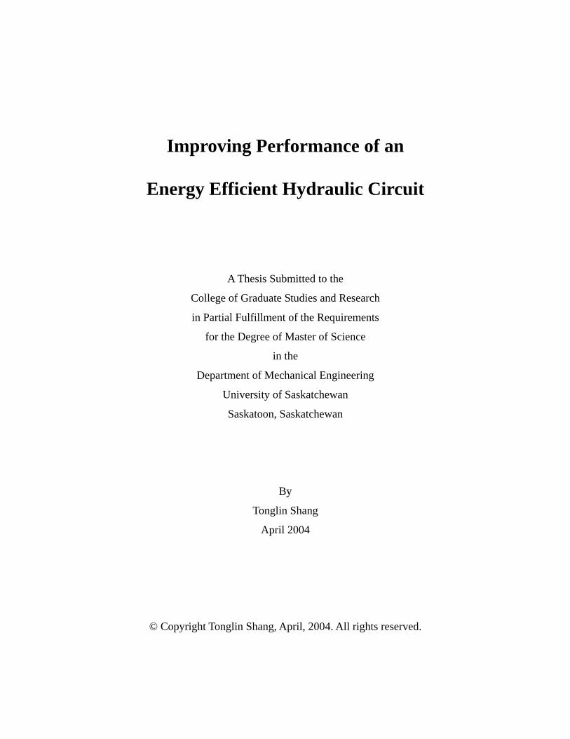
Figure 3.2 Critical gain and modified electrical time constant
3.1.4 Model Verification
The simulation results of the new model were compared with experimental results
which were previously measured. The same proportional gains and pressures were applied
to the new model under the same input conditions. Some typical results are shown in
Figure 3.3.
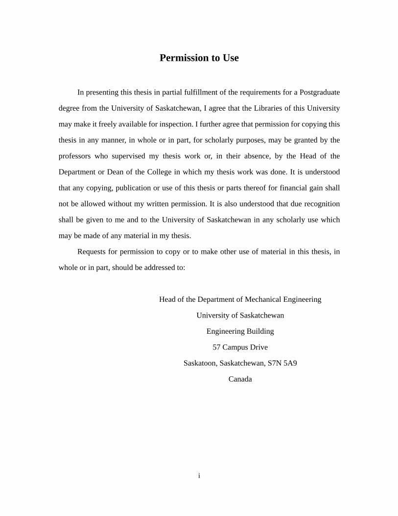
Figure 3.3(a) shows the dynamic response of the pump at a low pressure (3.45 MPa).
Both dynamic responses predicted by the simulation and measured approached the same
steady state after a transient period. However, the transient period of the measured pump
response ended in a relatively short time. This is compared with the measured response of
the pump in which the transient response of the simulation settled down after a longer time
period. When the proportional gain of the DC motor controller increased slightly from
0.19 to 0.21, both responses of the model simulation and experimental system exhibited
51
limit cycle oscillations (see Figure 3.3(c)). Figures 3.3(b) and (d) showed the dynamic
responses of the pump at a high pressure level (10.35 MPa). The results were similar to
those at the low pressure.
Figure 3.3 Comparison of measured swashplate angle and model prediction
It was observed that steady state values of the model simulation and experimental
test did not approach the desired swashplate angle. This was because the controller was a P
controller. The results shown in Figure 3.3 also indicated that dynamic response of the
model simulation did not match with those obtained experimentally in some aspects of the
performance. For example, when the pressure was low, the frequency of the limit cycle
oscillation was lower than that of the measured response; however, the oscillation
frequency was higher than the measured frequency when the pressure was high. A possible
cause for this phenomenon was the highly nonlinear characteristics of the pump system.
52
This made it impossible to include all factors which could affect the pump performance
into a simple model form.
Based on comparisons between model simulations and experimental tests, one
conclusion could be made for the model of the DC motor and pump: the model dynamic
response trends were “similar” to the physical system under the same loading conditions
and same input signal. “Similar” means that both the model prediction and physical
system output approached a common steady state value for smaller proportional gains and
demonstrated a limit cycle oscillation of similar frequency when increasing the
proportional gain to the critical gain (see Figure 3.3).
This characteristic of the model was important for the controller design of the DC
motor. As discussed previously, the objective of modeling was not to derive an accurate
model for the pump and DC motor. The model was mainly used to help the design of the
DC motor controller such that the DC motor controlled pump could work at different
loading conditions in a stable manner. As will be seen in the next section, the
Ziegler-Nichols tuning PID rules are used to design the controller. Ziegler-Nichols tuning
PID rules are only concerned with the critical gain and oscillation frequency for tuning the
controller gains. At this point, although this model was not an accurate representation of
the real system and the model prediction did not match the physical system very well, it
was considered to be “sufficient” for use in the preliminary controller design of the DC.
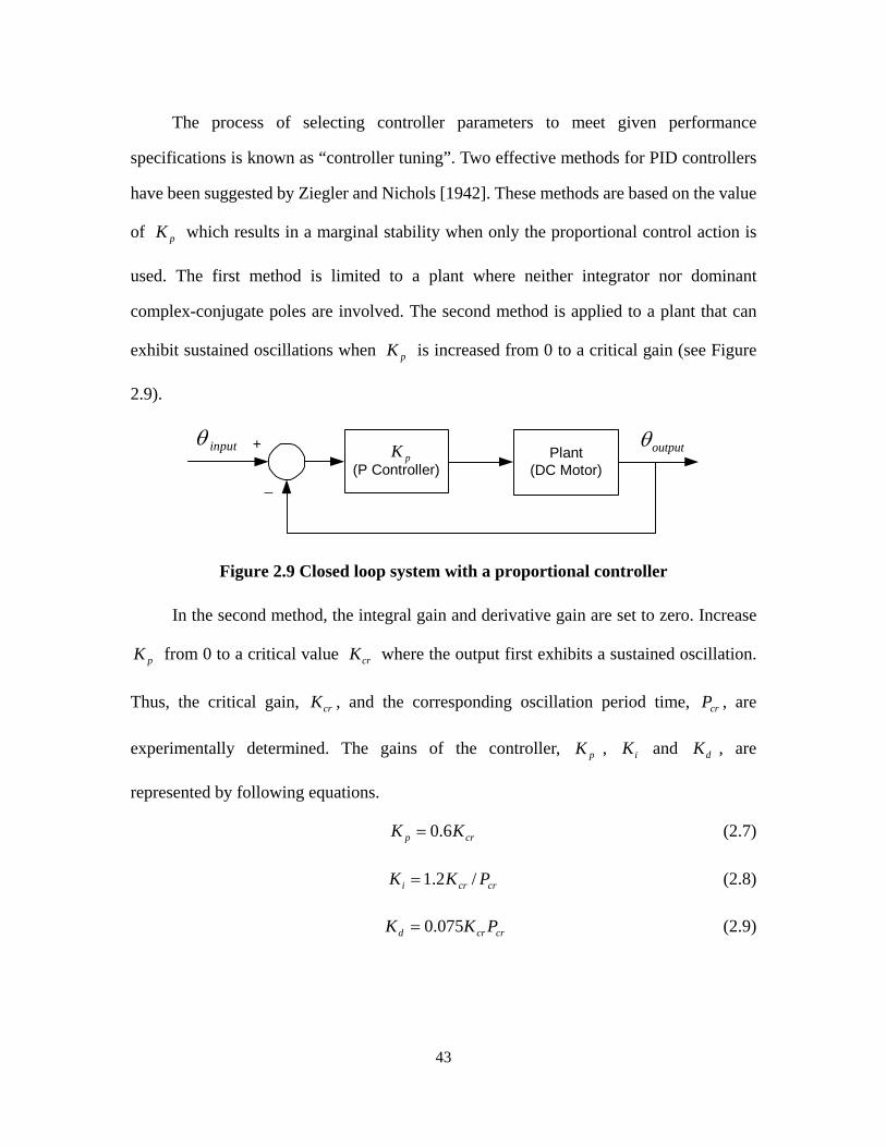
3.2 Nonlinear DC Motor Controller Design Based on the Model
This section will discuss the controller design based on the model of the DC motor
and pump. The requirement for the controller design at this stage was to design a DC
motor controller which could drive the DC motor and pump swashplate at any pressure
levels with a fast dynamic response but without exhibiting any limit cycle oscillations.
Many methods can be used to design the controller for a dynamic system; however,
most of them are limited to linear systems. According to the preliminary experience using
53
Ziegler-Nichols tuning PID rules (see Appendix B.3.2), it was found that these rules were
effective and convenient for the PID controller design, especially for the nonlinear DC
motor controlled pump system. The controller designed using these rules provided
satisfactory system performance. Hence, this method was also used as the basis of the
controller design based on the model of the DC motor and pump.
In order to design the motor controller using Ziegler-Nichols rules, a Matlab
program was written to calculate the critical gains and oscillation period time of the model
at different pressure levels and assist the controller design. The procedure is as follows:
1) For the linearized model of Appendix B, the coefficients were evaluated at
various operating points based on mathematical equations
2) The critical gain and oscillation period time were calculated at each operating
point. The results indicated that the critical gain and oscillation period time
were functions of the pressure.
3) PID controllers were designed at any pressure levels using the second
Method of Ziegler-Nichols tuning PID rules.
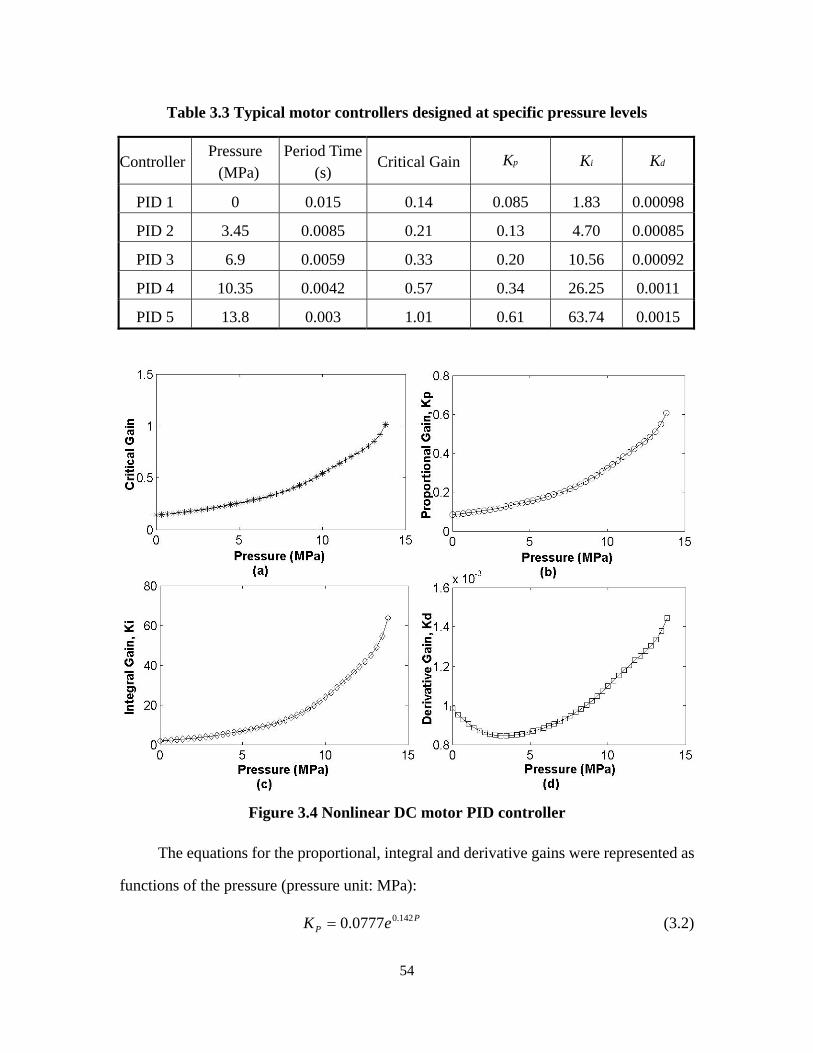
Table 3.3 presents parameters of some typical PID controllers which were designed
using this procedure at specific pressure levels.
It is to be noted that the controllers using the gains listed in Table 3.3 can only
properly function near the specified operating points. For example, the controller designed
for low pressure cannot work well at high pressure levels since the small gains do not
produce a fast dynamic response. Controllers designed at high-pressure levels have a fast
dynamic response at these levels, but they may exhibit sustained oscillations at
low-pressure levels.
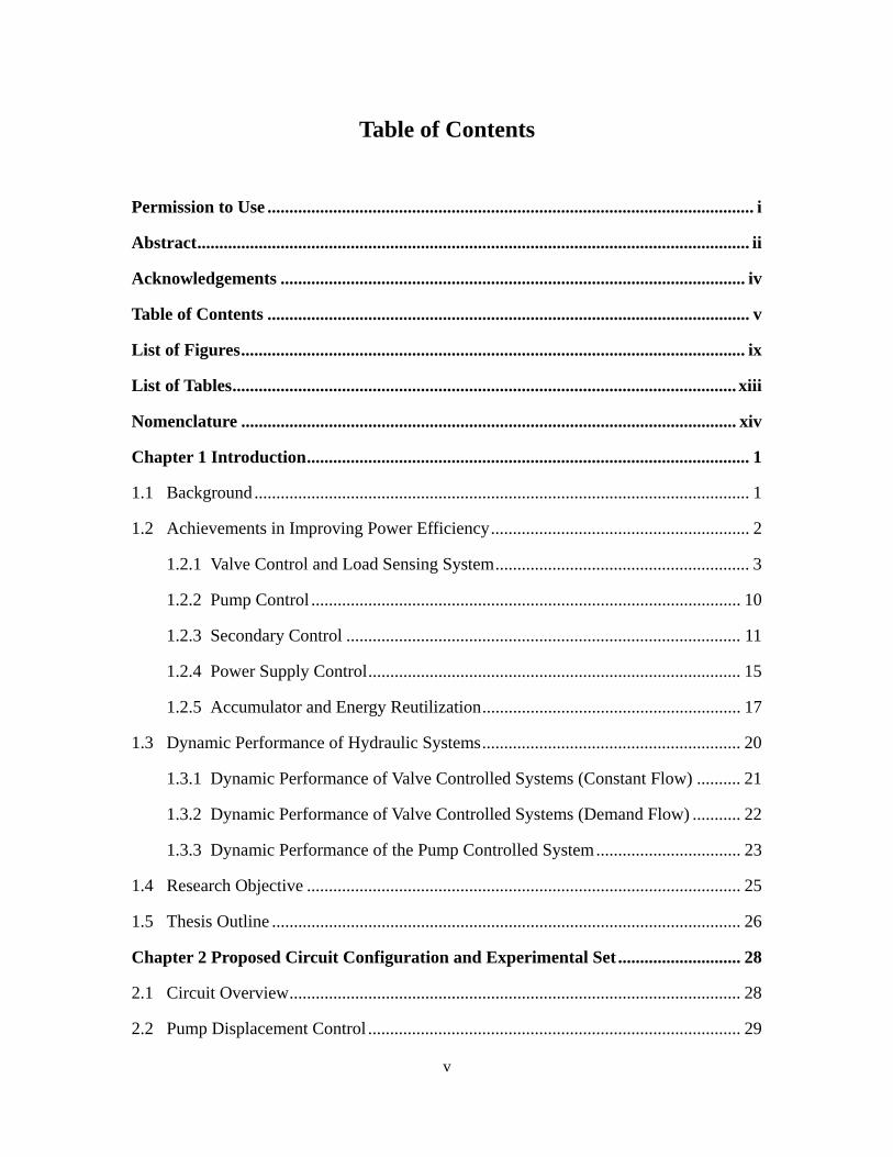
One solution to this problem was to design a nonlinear PID controller in which the
gains of the controller were a function of pressure. This was done by using a Matlab
program. Curves of the resulting PID gains as functions of the pressure are shown in
Figure 3.4.
54
Table 3.3 Typical motor controllers designed at specific pressure levels
Controller Pressure (MPa)
Period Time (s)
Critical Gain pK iK dK
PID 1 0 0.015 0.14 0.085 1.83 0.00098
PID 2 3.45 0.0085 0.21 0.13 4.70 0.00085
PID 3 6.9 0.0059 0.33 0.20 10.56 0.00092
PID 4 10.35 0.0042 0.57 0.34 26.25 0.0011
PID 5 13.8 0.003 1.01 0.61 63.74 0.0015
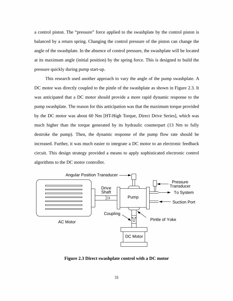
Figure 3.4 Nonlinear DC motor PID controller
The equations for the proportional, integral and derivative gains were represented as
functions of the pressure (pressure unit: MPa):
PP eK 142.00777.0= (3.2)
55
PI eK 251.0909.1= (3.3)
000943.01035.41075.5 526 +×−×= −− PPKD (3.4)
The controller designed was a variable PID controller which was pressure dependant.
It must be emphasized that the number of significant figures does not represent accuracy
of the experimental results but is a reflection of the program used to extract the function
from the data.
3.3 Experimental test of pump performance
To summarize, a variable displacement pump was controlled directly by a DC motor
attached to the swash plate of the pump. Through an iterative approach between
experimental testing and modeling, the model of the DC motor and pump was developed
and the controller of the DC motor designed off line using a variety of techniques. This
controller was now applied to the actual DC motor and pump system.
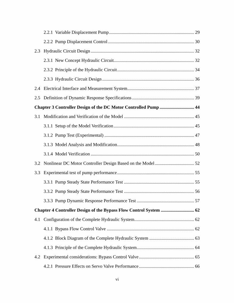
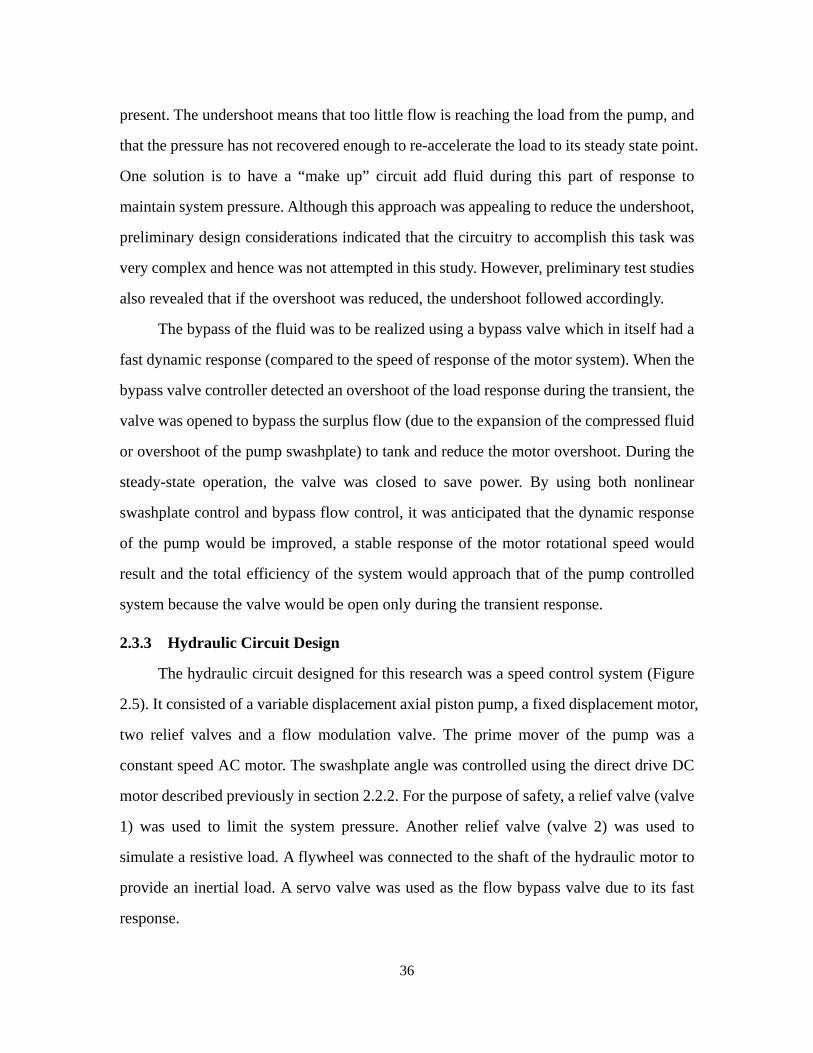
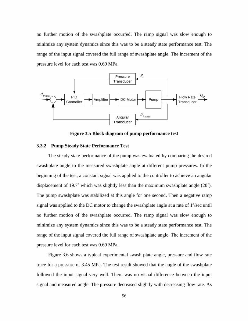
To evaluate the performance of the DC motor controlled pump, an experimental
system was designed to test the pump. As illustrated in Figure 3.5, it consisted of a
modified hydraulic pump, a DC motor, a DC motor amplifier and a closed-loop angle
control system. A pressure signal was fed back to the variable gain nonlinear controller. By
means of the controller designed in the previous section, the stroke of the pump can be
controlled in a stable fashion.
3.3.1 Pump Steady State Performance Test
The steady state performance of the pump was evaluated by comparing the desired
swashplate angle to the measured swashplate angle at different pump pressures. In the
beginning of the test, a constant signal was applied to the controller to achieve an angular
displacement of 19.7˚ which was slightly less than the maximum swashplate angle (20˚).
The pump swashplate was stabilized at this angle for one second. Then a negative ramp
signal was applied to the DC motor to change the swashplate angle at a rate of 1º/sec until
56
no further motion of the swashplate occurred. The ramp signal was slow enough to
minimize any system dynamics since this was to be a steady state performance test. The
range of the input signal covered the full range of swashplate angle. The increment of the
pressure level for each test was 0.69 MPa.
PumpDC Motor Flow RateTransducer
AngularTransducer
PressureTransducer
AmplifierinputPθ PQ
sP
PIDController
outputPθ
Figure 3.5 Block diagram of pump performance test
3.3.2 Pump Steady State Performance Test
The steady state performance of the pump was evaluated by comparing the desired
swashplate angle to the measured swashplate angle at different pump pressures. In the
beginning of the test, a constant signal was applied to the controller to achieve an angular
displacement of 19.7˚ which was slightly less than the maximum swashplate angle (20˚).
The pump swashplate was stabilized at this angle for one second. Then a negative ramp
signal was applied to the DC motor to change the swashplate angle at a rate of 1º/sec until
no further motion of the swashplate occurred. The ramp signal was slow enough to
minimize any system dynamics since this was to be a steady state performance test. The
range of the input signal covered the full range of swashplate angle. The increment of the
pressure level for each test was 0.69 MPa.
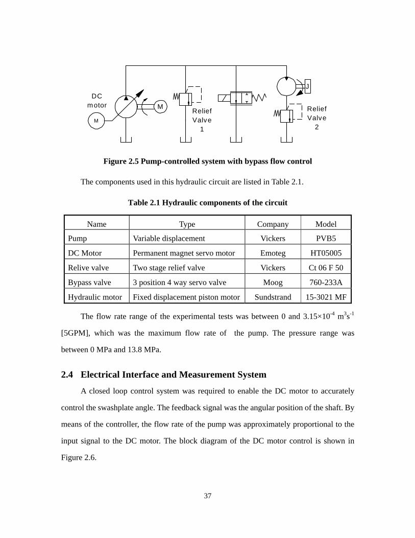
Figure 3.6 shows a typical experimental swash plate angle, pressure and flow rate
trace for a pressure of 3.45 MPa. The test result showed that the angle of the swashplate
followed the input signal very well. There was no visual difference between the input
signal and measured angle. The pressure decreased slightly with decreasing flow rate. As
57
the swashplate angle approached the zero position, the pressure and the flow rate quickly
decreased to zero. It was also observed that the relationship between the swashplate angle
and flow rate was not proportional. This phenomenon will be discussed in the next chapter.
The tests were highly repeatable at different pressures.
0
5
10
15
20
0 5 10 15 20Time (sec)
Ang
le (D
eg.)
and
Pres
sure
(MPa
)
0.00000
0.00010
0.00020
0.00030
0.00040
Flow
Rat
e (m
3/s)
Flow Rate
Pressure
Measured Angle
Figure 3.6 Measured steady state performance of the DC motor controlled pump
(A typical experimental test result)
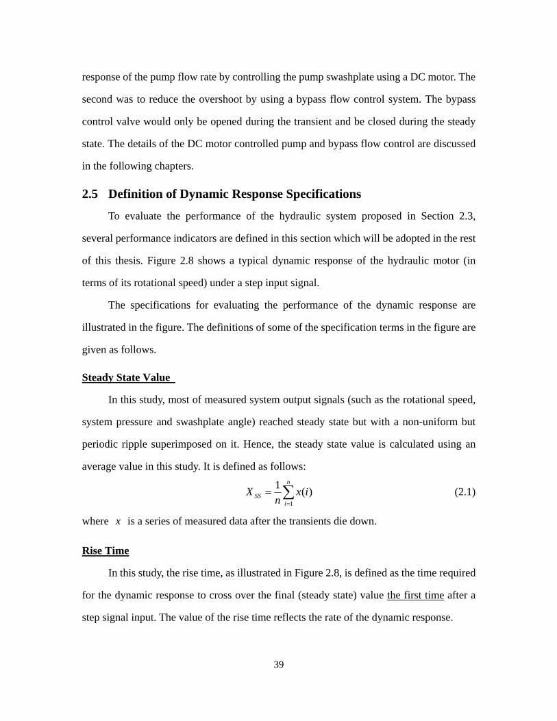
3.3.3 Pump Dynamic Response Performance Test
The dynamic performance of the pump can be established with a step input signal
test. Two important dynamic parameters, rise time and overshoot, can be measured from
this test. These terms are defined in Section 2.5. The test was realized by applying a step
input signal to the controller (similar to the steady state test) and was carried out at
different pressures.
The procedure for these tests was as follows:
1) The system pressure was adjusted by the main relief valve.
58
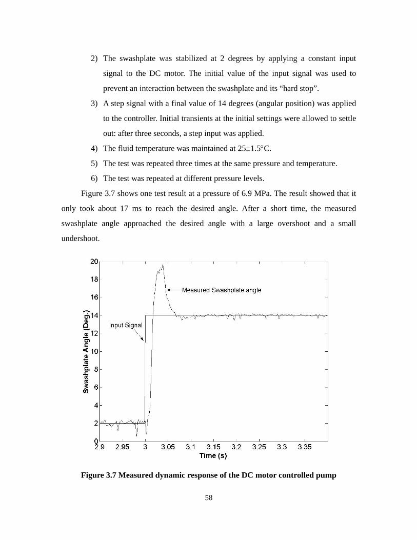
2) The swashplate was stabilized at 2 degrees by applying a constant input
signal to the DC motor. The initial value of the input signal was used to
prevent an interaction between the swashplate and its “hard stop”.
3) A step signal with a final value of 14 degrees (angular position) was applied
to the controller. Initial transients at the initial settings were allowed to settle
out: after three seconds, a step input was applied.
4) The fluid temperature was maintained at 25±1.5°C.
5) The test was repeated three times at the same pressure and temperature.
6) The test was repeated at different pressure levels.
Figure 3.7 shows one test result at a pressure of 6.9 MPa. The result showed that it
only took about 17 ms to reach the desired angle. After a short time, the measured
swashplate angle approached the desired angle with a large overshoot and a small
undershoot.
Figure 3.7 Measured dynamic response of the DC motor controlled pump
59
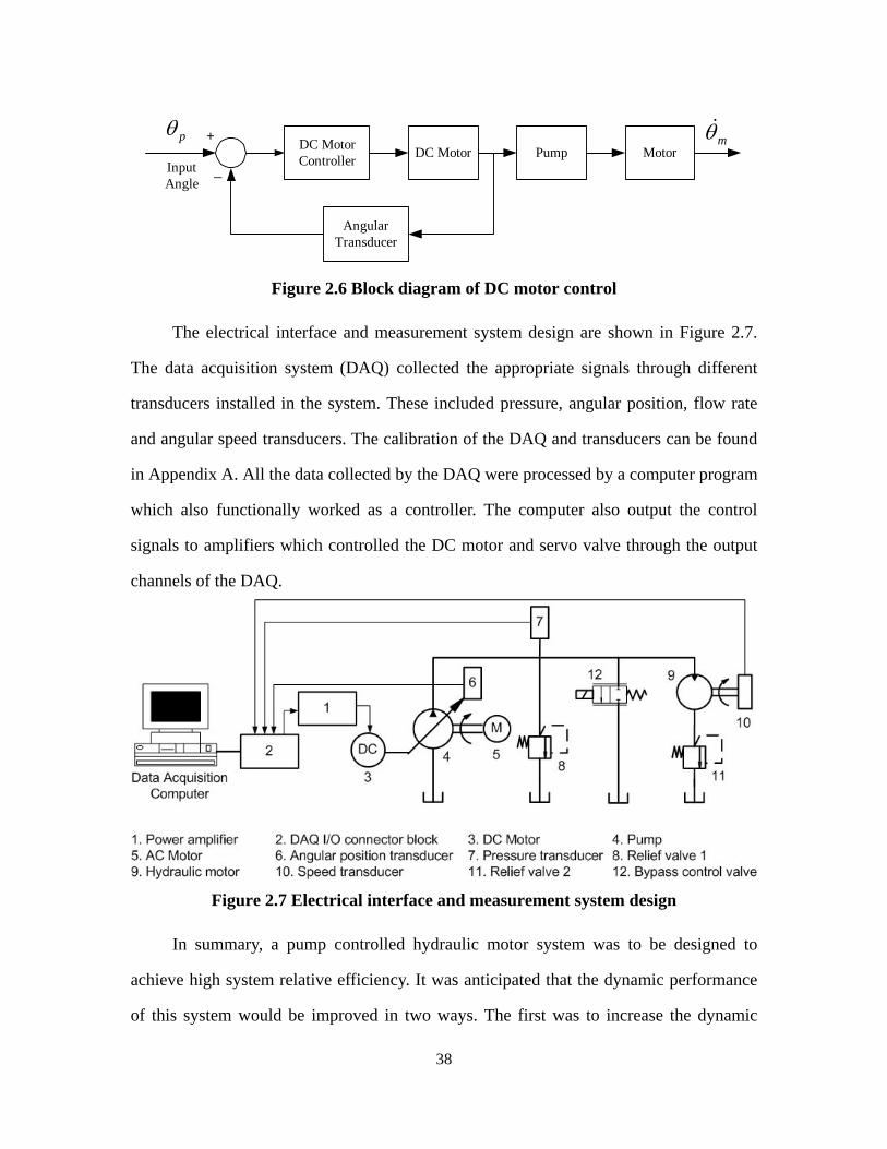
Since the rise time of the dynamic response was the main concern of the DC motor
controlled pump, the rise times of the swashplate angle were measured at different
pressure levels. Figure 3.8 shows the results of three tests and their average value. The rise
time varied between 15 and 35 ms depending on pressure levels. It was observed that the
rise time decreased with increasing pressure until the pressure reached 6.9 MPa and varied
slightly around 16 ms when the pressure was higher than 6.9 MPa.
0
5
10
15
20
25
30
35
40
45
0 2 4 6 8 10 12 14Pressure (MPa)
Ris
e Ti
me
of S
was
hpla
te A
ngle
(ms)
Rise time of test 1Rise time of test 2Rise time of test 3Average rise time
Test conditions1. Input signal: step input 2. Initial swashplate angle: 2 degrees2. Steady state value of the swashplate angle: 14 degrees
Figure 3.8 Rise time of pump swashplate angle with nonlinear PID controller
The test results shown in Figure 3.8 were measured only at one final swashplate
angle (14 degrees). The reason for choosing 14 degrees as the final swashplate angle for
all tests was that the swashplate could hit the hard stop for an swashplate angle larger than
14 degrees during the transient. If the swashplate hit the hard stop, the transient response
would be affected. As will be seen in Chapters 4 and 5, the final swashplate angle chosen
for these tests has the approximately same value for the tests conducted in those chapters.
The rise times of the swashplate measured at other final angular positions (not listed here)
showed a trend similar to the results shown in Figure 3.8; however, the values of the rise
time varied slightly depending on the angular positions. The rise time for a negative step
60
input signal was slightly larger than that of a positive signal since the pressure effect acting
on the swashplate was always in a direction of increasing swashplate angle.
All test results indicated that the DC motor controlled pump demonstrated a
relatively fast dynamic response (15-35 ms). This rise time can be compared to the 10 ms
rise time of typical relief valves [Yao, 1997], 30 – 60 ms of pressure actuated pumps [You,
1989] and 10 ms for the servo valve used in the bypass design [760 Series Servo valve,
Moog Inc.].
Figure 3.9 shows the overshoot and undershoot of the swashplate angle during the
transient. The undershoot of the response was small when compared with the overshoot.
At some pressure levels, the undershoot was quite small and in some cases, zero. The
overshoot varied between 30% and 50% and increased with increasing pressure. All
results shown in Figure 3.9 were calculated from the same tests, which were used for
calculating the rise time.
0
10
20
30
40
50
60
0 2 4 6 8 10 12 14Pressure (MPa)
Ove
rsho
ot a
nd U
nder
shoo
t (%
)
Overshoot of Test 1Overshoot of Test 2Overshoot of Test 3Average OvershootUndershoot of Test 1Undershoot of Test 2Undershoot of Test 3Average Undershoot
Overshoot
Undershoot
Figure 3.9 Overshoot and undershoot of pump swashplate angle
61
To summarize, the nonlinear DC motor controller could approach the steady state
value in a stable manner at different pressure levels. By means of this controller, the pump
exhibited a fast dynamic response with a rise time between 15 and 35 ms. However, the
pump also produced a large overshoot (30% to 50%). This overshoot will contribute to an
overshoot in the motor rotational speed response. This problem will be discussed in the
next chapter in which reducing the motor rotational speed overshoot is the main concern.
62
Chapter 4
Controller Design of the Bypass Flow Control System
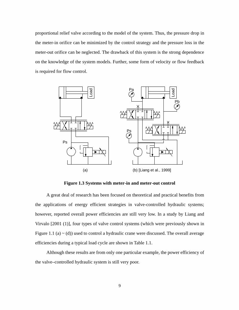
The design of the proposed bypass flow control system through a combination of
simulation and experimental studies is discussed in this chapter. First, the configuration
and operating principle of the bypass flow control system is presented. Some experimental
considerations related to the bypass control valve are also discussed. Then, a preliminary
controller is designed for the bypass control valve based on some experimental test results
on the hydraulic motor system. The performance of the preliminary controller is analyzed
and the structure of the controller modified and performance refined using simulation
studies. Finally, the feasibility of improving the dynamic performance of a speed control
system using the bypass flow control is examined using model simulation based on the
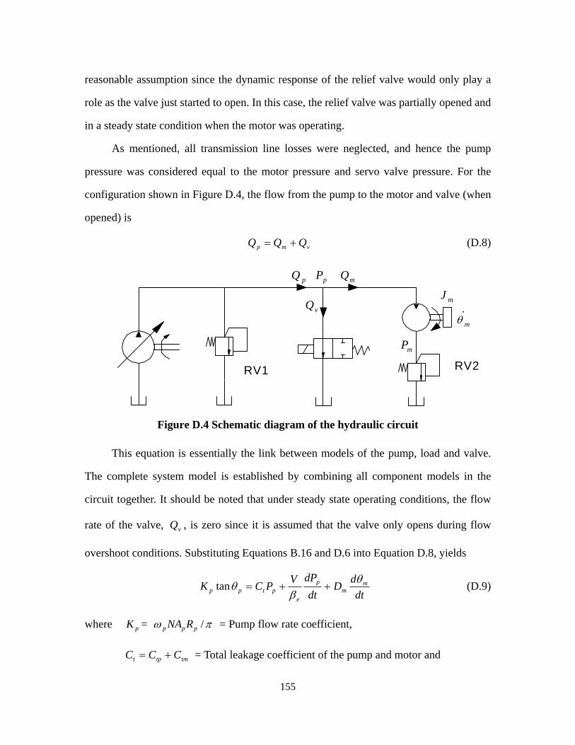
complete system model (see Appendix D).
4.1 Configuration of the Complete Hydraulic System
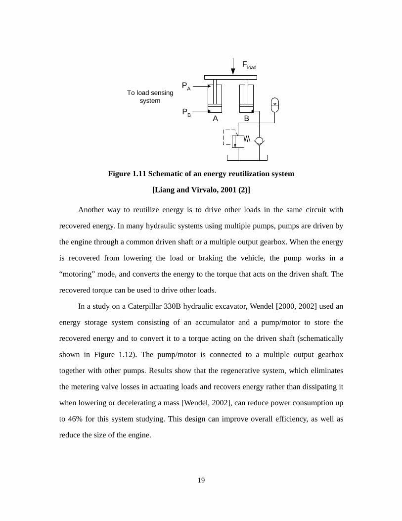
The complete hydraulic system proposed for this study was previously shown in
Figure 2.7. The main components of the system were a DC motor controlled variable
displacement pump, a bypass valve (servo valve) and a hydraulic motor. The DC motor
controlled pump was discussed in Chapter 3. This section will discuss the bypass control
valve and the complete hydraulic system.
4.1.1 Bypass Flow Control Valve
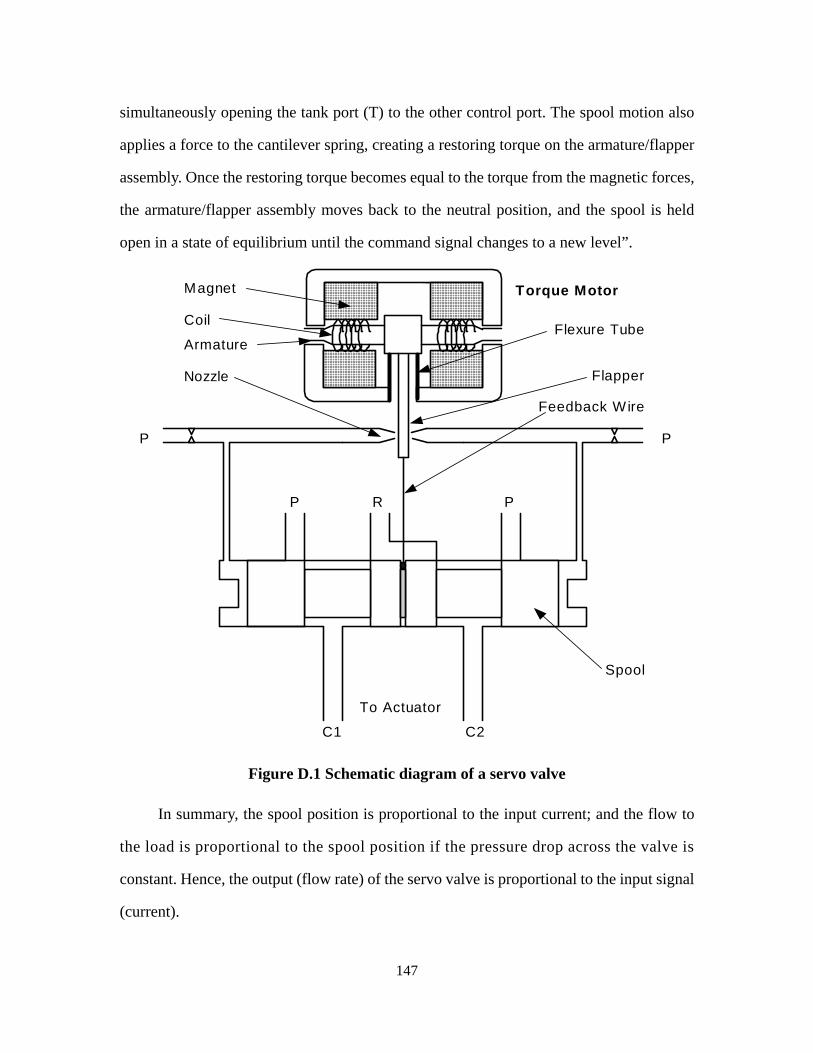
As previously mentioned, the purpose for using a bypass control valve was to
remove or minimize the overshoot associated with the overshoot of the pump swashplate
and the compressibility effects of the fluid, as seen by the hydraulic motor, during
transients. In order to achieve this target, the dynamic response of the bypass valve must
be “faster” than that of the pump. Servo valves, however, are known to show superior
63
dynamic responses compared to other modulation devices and have transient responses
comparable to the DC motor controlled pump. As mentioned in Section 3.3.2, the rise time
of the DC motor controlled pump was between 15 and 35 ms depending on the pump
pressure, and was less than 20 ms when the pressure was higher than 6.9 MPa. As will be
discussed in Section 4.2, the rise time of the servo valve was around 10 ms when the
pressure was higher than 6 MPa. Although the test conditions for the two systems were not
the same, the test results did demonstrate that the dynamic response of the servo valve was
faster than that of the DC motor controlled pump. Hence, this type of modulation device
was chosen for this application.
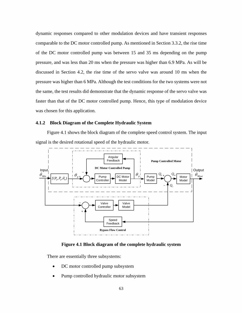
4.1.2 Block Diagram of the Complete Hydraulic System
Figure 4.1 shows the block diagram of the complete speed control system. The input
signal is the desired rotational speed of the hydraulic motor.
ValveController
ValveModel
SpeedFeedback
+
_
DC MotorModel
PumpModel
Minθ&),,( mpp PPf θ&& Pump
Controller
AngularFeedback
pQ mQpθ Motor
Model
vQ
_
+
_
+
Bypass Flow Control
DC Motor Controlled Pump
Pump Controlled Motor
pθInput Output
Moutθ&
Figure 4.1 Block diagram of the complete hydraulic system
There are essentially three subsystems:
• DC motor controlled pump subsystem
• Pump controlled hydraulic motor subsystem
64
• Bypass flow control subsystem
Although all these subsystems have been discussed previously, it is useful to briefly
discuss all three again but in terms of the overall system operation.
4.1.3 Principle of the Complete Hydraulic System
DC motor controlled pump subsystem
The pump subsystem is a closed loop system including a nonlinear PID controller, a
power amplifier, a DC motor and a variable displacement pump. The feedback signal is
the angular position of the pump swashplate, which is also the controlled variable.
Changing the swashplate angle can vary the pump displacement. The purpose for
controlling the swashplate angle is to control the flow rate of the pump.
Pump Controlled Hydraulic Motor Subsystem
This subsystem includes the DC motor controlled pump subsystem. The input signal
is the desired rotational speed of the hydraulic motor ( mθ& ), and the output signal is the
actual rotational speed of the hydraulic motor. The principle of the pump controlled
hydraulic motor system is as follows: First, assuming ideal conditions, the rotational speed
input signal is converted to a desired pump swashplate angle ( pθ ) using the hydraulic
system model (see Equation D.10). Then, this swashplate angle is fed into the DC motor
controller to locate the swashplate to a desired angle. Finally the pump supplies the
hydraulic motor with the required flow by which the hydraulic motor generates a
rotational speed approximately proportional to the input rotational speed.
Bypass Flow Control Subsystem
This is a closed loop system. The controlled variable is the speed of the hydraulic
motor ( mθ& ). The input signal is the same as that of the pump controlled hydraulic motor
system. The rotational speed signal of the hydraulic motor is fed back to the input of the
65
valve controller. The bypass flow control is used to remove the excess flow from the pump
if the motor rotational speed is larger than the desired rotational speed. This can occur
under the condition when the motor exhibits a large overshoot during the transient
response. In this case, the bypass flow control algorithm is designed to minimize the
overshoot.
Principle of the Complete System
The operation of the complete system is as follows. First, the desired rotational
speed of the hydraulic motor is converted to the pump swashplate angle (via Equation
D.10). Then, the DC motor drives the pump swashplate to achieve this desired angle in the
shortest time possible. Accordingly, the pump supplies the appropriate flow rate to drive
the hydraulic motor. During the whole operation, the bypass flow control system monitors
the rotational speed of the hydraulic motor and takes an appropriate control action when
the motor rotational speed exceeds the desired rotational speed. Finally, because of the
improved dynamic response of the DC motor controlled pump, the desired rotational
speed of the hydraulic motor should be achieved with an improved dynamic response as
well; the performance of the hydraulic motor would be further improved with a reduction
in the overshoot due to the bypass valve.
The overall system is not a closed loop system since the motor rotational speed
signal is not directly fed back to the main input of the system.
4.2 Experimental considerations: Bypass Control Valve
Before a controller for the bypass control valve could be developed, preliminary
investigations revealed some peculiarities associated with the operation and configuration
of the servo valve so chosen. This section will consider some of these characteristics as
they play an important role in the final design of the controller. The process was one of
experimentally evaluating the performance of the valve under variety of pressure
66
conditions and examining some preliminary controllers experimentally for the bypass
system. Based on the results of these preliminary tests, a controller was then designed
using an experimental approach and modified using model simulation.
To use the servo valve as a bypass flow control valve, some properties of the servo
valve had to be investigated before designing the valve controller and experimental system.
They were:
• The effect of the pressure drop across the bypass valve on its dynamic
performance.
• How to install a servo valve as a bypass flow control valve.
These two questions arose due to the special properties of the bypass control
configuration and servo valve structure. These questions are addressed in the following
sections.
4.2.1 Pressure Effects on Servo Valve Performance
Servo valves are normally used in hydraulic circuits in which the supply pressure is
constant and with the aid of feedback or pressure compensation, they can be used to
control flow. As discussed in Appendix D.1, the pilot stage of the servo valve was a
flapper valve. To make the flapper valve work properly, the fluid that came from the
nozzles and acted on the flapper had to be maintained at a certain pressure level. Thus, the
supply pressure from which the nozzle was fed, had to be maintained greater than a
specified value. For Moog760 valve used in this study, the pressure drop across the valve
is required to be greater than 6.9 MPa to get the best performance. However, in this study,
the supply pressure of the valve was the same as the system pressure, and was not constant
but varied with changes in loading conditions.
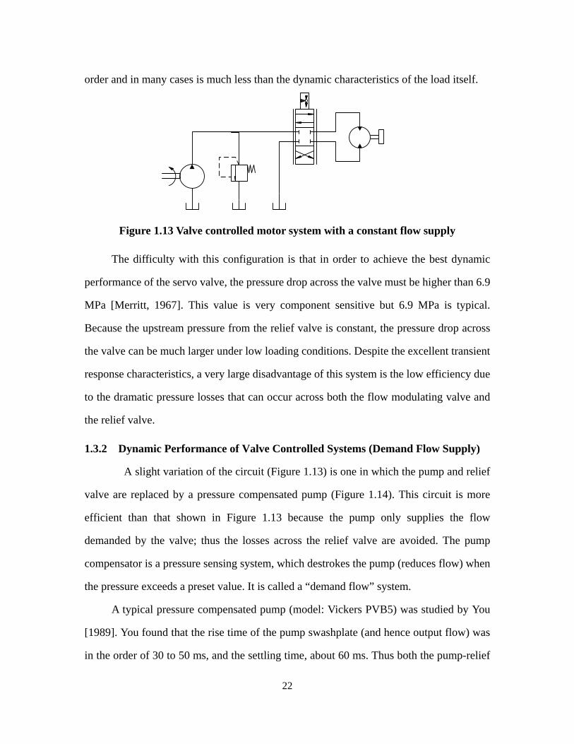
To test how the pressure drop across the valve affected the dynamic performance of
the actual valve, (especially when the pressure drop was less than the specified value), an
experimental test was designed to determine the transient response of the valve in terms of
67
flow rate under different pressure levels. The circuit is shown in Figure 4.2. The relief
valve was used to adjust the pressure drop across the valve. A flow rate transducer was
installed to measure the flow rate through the valve. The pump delivered the maximum
flow rate (19 l/min).
M
Flow rate transducer
Servo Valve
Relief valve
Figure 4.2 Hydraulic circuit for testing the servo valve performance
In the first instance, the bypass valve was closed and hence all the pump flow was
over the relief valve at the set pressure. A simple PID controller was designed for the servo
valve using Ziegler-Nichols rules. The controller was designed for a supply pressure of 6.9
MPa. This controller was not meant to be the final controller for the bypass control valve.
It was only used for this particular test.
The procedure for measuring the flow rate of the valve during the transient was as
follows:
1) A step input signal was applied to the servo valve and the flow rate measured.
2) The test supply pressure was increased by adjusting the relief valve from 0.69
MPa to 7.6 MPa in increments of 0.69 MPa.
3) The test was repeated with the temperature kept approximately constant
(25±1.5°C).
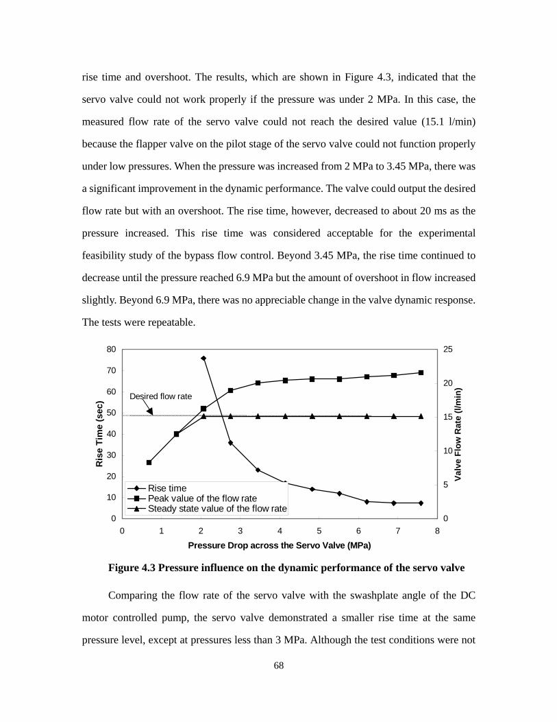
The dynamic responses at different pressure levels were evaluated in terms of the
68
rise time and overshoot. The results, which are shown in Figure 4.3, indicated that the
servo valve could not work properly if the pressure was under 2 MPa. In this case, the
measured flow rate of the servo valve could not reach the desired value (15.1 l/min)
because the flapper valve on the pilot stage of the servo valve could not function properly
under low pressures. When the pressure was increased from 2 MPa to 3.45 MPa, there was
a significant improvement in the dynamic performance. The valve could output the desired
flow rate but with an overshoot. The rise time, however, decreased to about 20 ms as the
pressure increased. This rise time was considered acceptable for the experimental
feasibility study of the bypass flow control. Beyond 3.45 MPa, the rise time continued to
decrease until the pressure reached 6.9 MPa but the amount of overshoot in flow increased
slightly. Beyond 6.9 MPa, there was no appreciable change in the valve dynamic response.
The tests were repeatable.
0
10
20
30
40
50
60
70
80
0 1 2 3 4 5 6 7 8
Pressure Drop across the Servo Valve (MPa)
Ris
e Ti
me
(sec
)
0
5
10
15
20
25
Valv
e Fl
ow R
ate
(l/m
in)
Rise timePeak value of the flow rateSteady state value of the flow rate
Desired flow rate
Figure 4.3 Pressure influence on the dynamic performance of the servo valve
Comparing the flow rate of the servo valve with the swashplate angle of the DC
motor controlled pump, the servo valve demonstrated a smaller rise time at the same
pressure level, except at pressures less than 3 MPa. Although the test conditions were not
69
the same for both systems, the comparison results showed that the servo valve had a faster
dynamic response and should be able to accommodate the overshoot of the hydraulic
motor.
As seen from Figure 4.3, the dynamic performance of the valve would be adversely
affected if the pressure were low. To maintain an acceptable performance, a minimum
pressure drop across the valve should be around 3.45 MPa. For the experimental system
shown in Figure 2.7, it was possible to build up this pressure because of a combination of
the friction in the hydraulic motor (which resulted in pressures of 1.5~2.5 MPa depending
on the rotational speed), and the relief valve, RV2 (which could be used to adjust the motor
backpressure and increase the system pressure to an acceptable level).
It should be noted that this pressure limitation is not a necessarily a constraint on the
bypass flow control concept but is a constraint on the servo valve used in the study. As
discussed in the next Section, a suitable two way valve was not available in the lab so the
servo valve had to be used.
4.2.2 Installation of the Servo Valve
The installation of the bypass valve in a bypass flow control system is different from
that in a normal flow control system. This configuration makes the design of the controller
for the bypass flow control complex. In this section, how the installation of the bypass
control valve affects the controller design is discussed.
Ideally, the proposed bypass flow control valve should be a two-way, closed
centered device. From a practical point of view, a two-way high-speed valve was not
available in the lab, so a four-way servo valve (described in Section 4.1.1) was used to
serve this purpose. The four-way valve had four ports to connect to the hydraulic circuit;
however, for the bypass flow control, only two ports were used. How to handle the other
two ports of the servo valve was an issue that had to be carefully addressed.
Figure 4.4 shows 3 possible installations of the servo valve. In Figure 4.4(a), port
70
“T” and port “C2” are blocked. When the spool moves to the left valve position, pressure
port “P” will be connected to port “C1”. When the spool moves to the right, pressure port
“P” will be blocked by port “C2”. Theoretically, this configuration should be sufficient to
simulate a two-way valve operation. However, the physical internal design of the valve
makes this scenario impossible to implement. The flow from the pilot stage cannot make
its way back to tank if the “T” port is blocked. Thus the valve cannot function properly.
(c)(b)(a)
L R
P T
C1 C2
pQ pP mQ
vQ
pQ pP mQ
vQ
pQ pP mQ
vQ
Figure 4.4 Installations of the servo valve
In Figure 4.4(b), pressure port “P’ is always connected to the port “T”, regardless if
the spool moves to the left or right position. This configuration could create some
difficulties when it comes to controller design. For a regular control system, different input
signals generate distinctly different outputs. However, for the servo valve shown in Figure
4.4(b), a positive and negative input signal of the same value will produce the same output
which could create problems in terms of controller design.
Consider Figure 4.4(c). The port “T” is connected to tank and port “C2” is blocked.
In this configuration, if the spool is moved to the left position, then the fluid is bypassed to
tank. Assuming that a positive signal will move the spool to its left position, then the
bypassed flow rate will be proportional to the applied positive signal (pressure drop being
assumed constant). For a negative signal, the valve spool moves to the right position
(Figure 4.4(c)) and the flow is blocked for all negative signal inputs. The flow from the
pilot stage can go back to the tank through the “T” port. This particular valve
71
configuration was feasible for bypass flow control.
Although it is unusual to use a servo valve in this mode, preliminary test results
indicated that the high dynamic bandwidth of the servo valve in a four-way mode was not
compromised with this particular arrangement.
4.3 Bypass Flow Control Design
The objective of this section is to present the design of a controller for the bypass
flow control valve. The main steps for the controller design were as follows. First, a
preliminary controller for the bypass control valve was designed in an experimental
operating mode. Some difficulties were experienced with this controller and thus, an
attempt was made to determine the cause of the problem based on the simulation of the
bypass valve and motor models. Finally, the controller was modified using the simulation
results and applied to the complete model of the system for “proof of concept”. The
following sections will present the process used to design the bypass valve controller.
4.3.1 Controller Design of the Bypass Control Valve (Experimental Approach)
The experimental system showing the motor with the bypass valve was previously
shown in Figure 2.7; in this case, the flywheel was not attached to the motor. The system
backpressure (and hence the upstream valve pressure) was set to 4 MPa by adjusting the
relief valve installed after the hydraulic motor. At full stroke, the pump delivered the
maximum flow rate of 19 l/m. Only one system pressure was considered (4 MPa) for the
preliminary valve controller design. It was anticipated that the controller designed at this
pressure level could provide a fast and stable dynamic response for most of the loading
conditions expected. The reason for this assumption was that the servo valve demonstrated
a comparatively fast dynamic response with a rise time less than 20 ms when the pressure
was higher than 4 MPa (as shown in Figure 4.3). Hence, the controller designed at this
pressure level should, at least, provide the same dynamic performance at high pressure
72
levels.
The design procedure for the bypass valve controller was quite similar to that for the
design of the DC motor controller discussed in Section 3.2; thus, the experimental test and
design procedures will not be repeated. The critical gain and oscillation period time were
measured by increasing the proportional gain of the bypass valve controller until the
hydraulic motor exhibited a limit cycle oscillation. The critical gain ( crK ) was determined
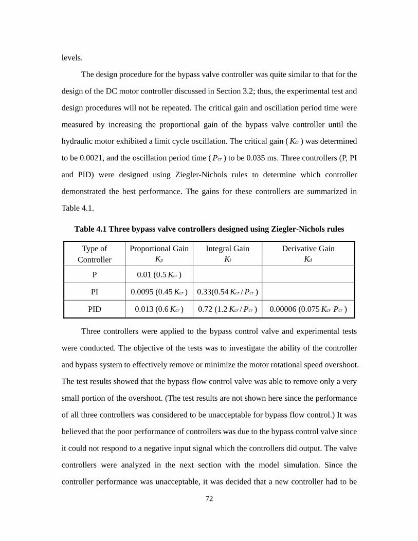
to be 0.0021, and the oscillation period time ( crP ) to be 0.035 ms. Three controllers (P, PI
and PID) were designed using Ziegler-Nichols rules to determine which controller
demonstrated the best performance. The gains for these controllers are summarized in
Table 4.1.
Table 4.1 Three bypass valve controllers designed using Ziegler-Nichols rules
Three controllers were applied to the bypass control valve and experimental tests
were conducted. The objective of the tests was to investigate the ability of the controller
and bypass system to effectively remove or minimize the motor rotational speed overshoot.
The test results showed that the bypass flow control valve was able to remove only a very
small portion of the overshoot. (The test results are not shown here since the performance
of all three controllers was considered to be unacceptable for bypass flow control.) It was
believed that the poor performance of controllers was due to the bypass control valve since
it could not respond to a negative input signal which the controllers did output. The valve
controllers were analyzed in the next section with the model simulation. Since the
controller performance was unacceptable, it was decided that a new controller had to be
73
considered and that the best approach would be to redesign this controller based on the
model simulation of the servo valve, hydraulic motor and valve controller.
4.3.2 Analysis of the Bypass Flow Control (Simulation)
In a normal closed loop system, a controller must respond to a complete range of
input signals, which includes both positive and negative values. However, this general rule
cannot be applied to the bypass flow control since, as discussed in Section 4.2.2, the valve
does not respond to a negative input signal. This property has a significant influence on the
design of the bypass valve controller.
In order to analyze how the bypass flow control design was affected by this property,
a simulation was developed based on models of the servo valve and hydraulic motor
which are developed in Appendix D. The block diagram is shown in Figure 4.5.
ValveController
AmplifierModel
ValveModel
MotorModel
mθ&
+
_
+
_
pQ
vQ
mQPump
Input
mθ&
Output
Figure 4.5 Block diagram of bypass flow control system
This block diagram is a part of the complete system block diagram shown in Figure
4.1. To design this closed bypass flow control system, the rotational speed output signal of
the hydraulic motor was fed back to the input of the servo valve. The negative sign on the
input desired rotational speed and the positive sign of the motor rotational speed was to
accommodate the fact that a negative (subtraction) flow was required during the bypass
mode. A signal conditioner block was designed to restrict the output of the valve to only
positive values (ie, bypass flow was viewed by the system as negative flow). This block
74
was used to simulate the uniqueness of the bypass valve which could only response to a
positive input signal.
The purpose of using the bypass control valve was to reduce the overshoot of the
hydraulic motor rotational speed. To analyze the performance of the bypass flow control
system, a simulation was conducted first by applying three valve controllers (listed in
Table 4.1) to the model of the bypass control valve. The simulation conditions are as
follows:
• The input signal was a desired constant rotational speed signal (100 rad/s).
• A sine wave with a magnitude of 10 rad/s and a bias signal of 2 rad/s were
superimposed on the input signal to simulate an overshoot and undershoot
condition.
• The system-simulated pressure was 4 MPa (same as the pressure in the
experimental test).
By means of this input signal combination, the pump was assumed to supply a flow
rate which was equivalent to a motor rotational speed of 100 rad/s with an overshoot of
12% and an undershoot of 8%. For the pump, this was a steady state response. However,
from the viewpoint of the bypass control valve, it was considered to be a dynamic
response because effective flow rate of the pump simulated overshoot and undershoot
conditions.
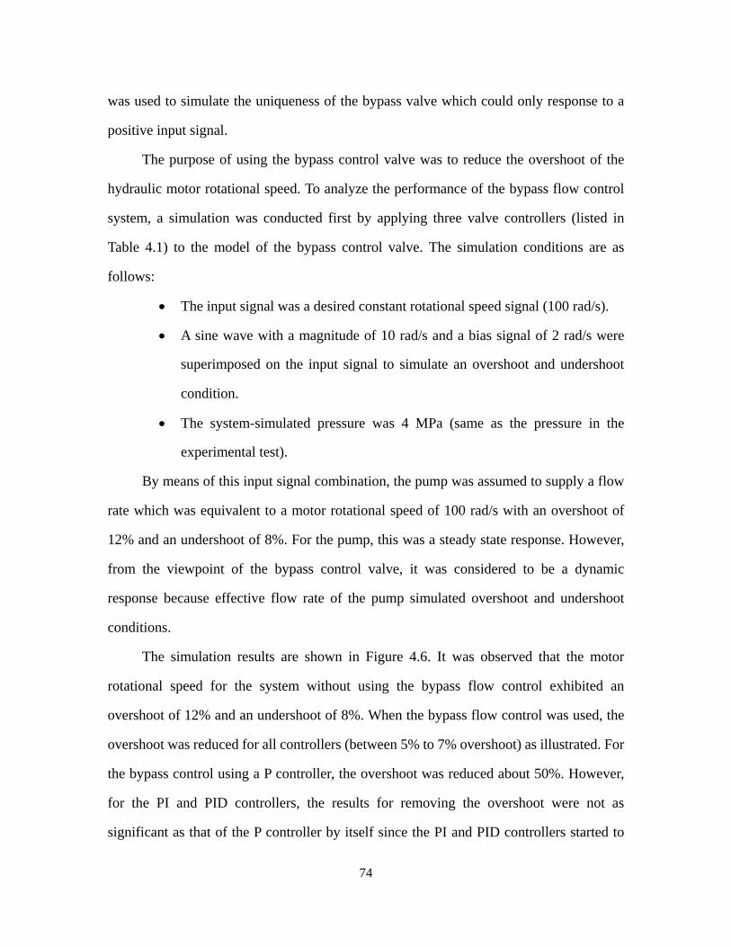
The simulation results are shown in Figure 4.6. It was observed that the motor
rotational speed for the system without using the bypass flow control exhibited an
overshoot of 12% and an undershoot of 8%. When the bypass flow control was used, the
overshoot was reduced for all controllers (between 5% to 7% overshoot) as illustrated. For
the bypass control using a P controller, the overshoot was reduced about 50%. However,
for the PI and PID controllers, the results for removing the overshoot were not as
significant as that of the P controller by itself since the PI and PID controllers started to
75
take corrective actions after a time delay. Theoretically, for linear systems, the PI and PID
controllers should have produced better results when compared with the P controller. A
possible cause for this situation was that the integrator of the PI and PID controllers could
not take the proper action in a bypass flow control system; this was an issue that had to be
addressed before any controller could be reliably and effectively applied to the
experimental system.
Figure 4.6 Valve controller performances
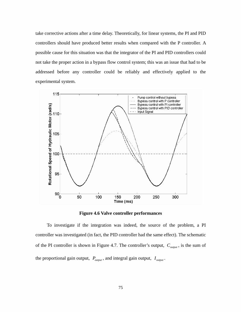
To investigate if the integration was indeed, the source of the problem, a PI
controller was investigated (in fact, the PID controller had the same effect). The schematic
of the PI controller is shown in Figure 4.7. The controller’s output, outputC , is the sum of
the proportional gain output, outputP , and integral gain output, outputI .
76
+
_inputmθ&pK
ski
mθ&∆
outputP
outputI
outputC
Motor Rotational Speed
Valve ModelInput signalPI Controller
outputmθ&
Figure 4.7 Schematic of the PI controller
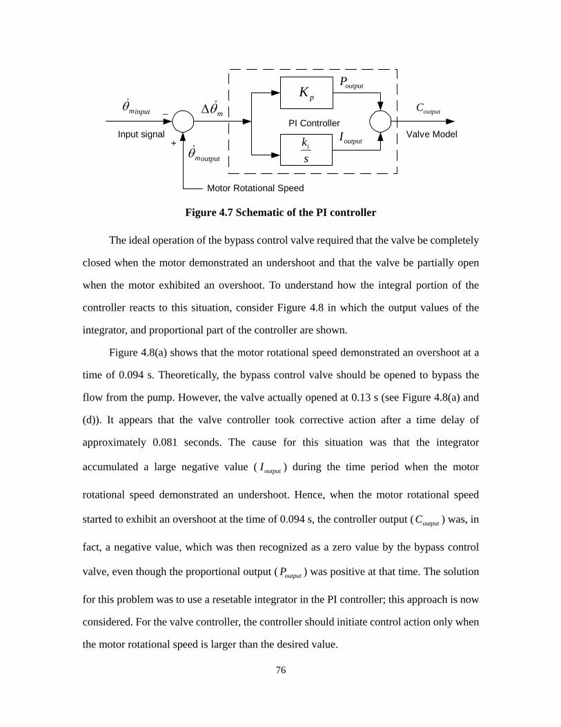
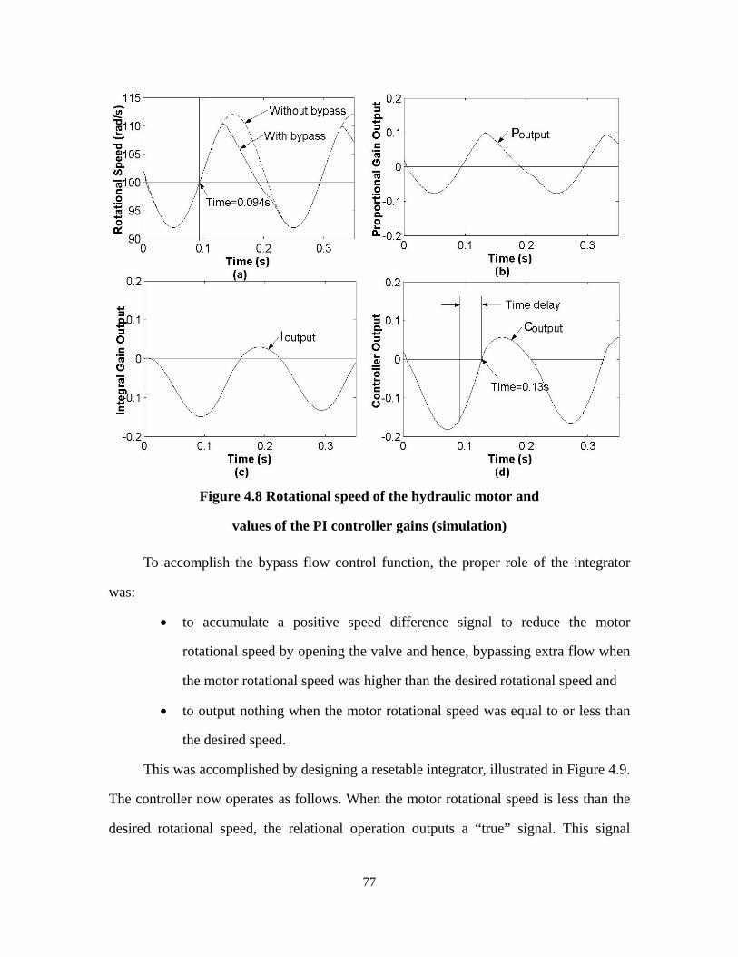
The ideal operation of the bypass control valve required that the valve be completely
closed when the motor demonstrated an undershoot and that the valve be partially open
when the motor exhibited an overshoot. To understand how the integral portion of the
controller reacts to this situation, consider Figure 4.8 in which the output values of the
integrator, and proportional part of the controller are shown.
Figure 4.8(a) shows that the motor rotational speed demonstrated an overshoot at a
time of 0.094 s. Theoretically, the bypass control valve should be opened to bypass the
flow from the pump. However, the valve actually opened at 0.13 s (see Figure 4.8(a) and
(d)). It appears that the valve controller took corrective action after a time delay of
approximately 0.081 seconds. The cause for this situation was that the integrator
accumulated a large negative value ( outputI ) during the time period when the motor
rotational speed demonstrated an undershoot. Hence, when the motor rotational speed
started to exhibit an overshoot at the time of 0.094 s, the controller output ( outputC ) was, in
fact, a negative value, which was then recognized as a zero value by the bypass control
valve, even though the proportional output ( outputP ) was positive at that time. The solution
for this problem was to use a resetable integrator in the PI controller; this approach is now
considered. For the valve controller, the controller should initiate control action only when
the motor rotational speed is larger than the desired value.
77
Figure 4.8 Rotational speed of the hydraulic motor and
values of the PI controller gains (simulation)
To accomplish the bypass flow control function, the proper role of the integrator
was:
• to accumulate a positive speed difference signal to reduce the motor
rotational speed by opening the valve and hence, bypassing extra flow when
the motor rotational speed was higher than the desired rotational speed and
• to output nothing when the motor rotational speed was equal to or less than
the desired speed.
This was accomplished by designing a resetable integrator, illustrated in Figure 4.9.
The controller now operates as follows. When the motor rotational speed is less than the
desired rotational speed, the relational operation outputs a “true” signal. This signal
78
triggers the resetable integrator and resets the accumulated previous rotational speed
difference signal to zero. The output of the PID controller is now zero or negative. The
valve is closed and the motor keeps running at a rotational speed which matches the pump
flow rate. If the pump cannot supply enough flow to drive the motor during the dynamic
transient, the motor rotates at a relatively slower rotational speed and exhibits an
undershoot. In this case, the bypass flow control system cannot contribute to a direct
reduction in the undershoot of the motor. If the motor rotational speed is higher than the
desired speed, the relational operation will output a “false” signal, which in turn will not
trigger the resetable integrator. In this case, the PID controller works as a regular PID
controller.
+
_
0≤
pK
sK d
skiyes
Valveinputmθ
&
outputmθ&
Figure 4.9 Schematic of a “resetable” PID controller
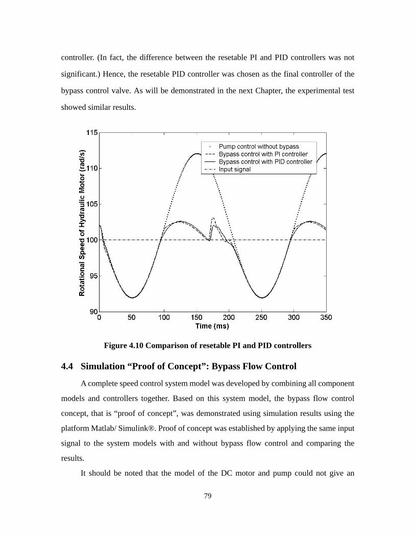
To test if the resetable integrator did indeed, improve performance, the simulation
was reexamined with both the resetable PI and PID controllers and the results are shown in
Figure 4.10 using the same simulation conditions as mentioned previously. The simulation
results for the model without using the bypass are also shown in the same figure for
comparison.
The result indicated that the improvement in reducing the overshoot was significant
by using the resetable integrator strategy. When comparing the performances of two
controllers, the resetable PID controller behaved marginally better than the resetable PI
79
controller. (In fact, the difference between the resetable PI and PID controllers was not
significant.) Hence, the resetable PID controller was chosen as the final controller of the
bypass control valve. As will be demonstrated in the next Chapter, the experimental test
showed similar results.
Figure 4.10 Comparison of resetable PI and PID controllers
4.4 Simulation “Proof of Concept”: Bypass Flow Control
A complete speed control system model was developed by combining all component
models and controllers together. Based on this system model, the bypass flow control
concept, that is “proof of concept”, was demonstrated using simulation results using the
platform Matlab/ Simulink®. Proof of concept was established by applying the same input
signal to the system models with and without bypass flow control and comparing the
results.
It should be noted that the model of the DC motor and pump could not give an
80
accurate prediction for the system output during the whole load range due to nonlinear
characteristics of the system. But, it could indeed give good predictions at some operating
points if a few minor modifications were made to the model parameters. Hence, the model
of the DC motor and pump was still used to test the overall “Proof of concept” on the
whole system, but only used at operating points which were experimentally verified.
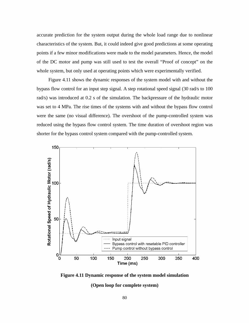
Figure 4.11 shows the dynamic responses of the system model with and without the
bypass flow control for an input step signal. A step rotational speed signal (30 rad/s to 100
rad/s) was introduced at 0.2 s of the simulation. The backpressure of the hydraulic motor
was set to 4 MPa. The rise times of the systems with and without the bypass flow control
were the same (no visual difference). The overshoot of the pump-controlled system was
reduced using the bypass flow control system. The time duration of overshoot region was
shorter for the bypass control system compared with the pump-controlled system.
Figure 4.11 Dynamic response of the system model simulation
(Open loop for complete system)
81
In summary, this section has established “proof of concept” for the bypass flow
control approach. The simulation results show that the proposed approach can improve the
dynamic performance of the hydraulic motor by reducing the overshoot of the motor
rotational speed.
82
Chapter 5
Experimental Verification of the
Bypass Flow Control Concept
The controllers of the DC motor and bypass valve were designed and tested in
previous chapters. Based on these controllers and the model of the complete hydraulic
system, a simulation of the bypass flow control circuit was completed and used to
establish the theoretical “proof of concept”; in addition, the model was used as an aid in
the design of the bypass controller. This chapter will:
• Consider the pump-controlled hydraulic motor system with the bypass flow
control,
• Examine the measurements of the dynamic responses of the system with and
without the bypass flow control under different loading conditions and,
• Evaluate and discuss the test results according to the objective of this study.
5.1 General
5.1.1 Objective of the Test
As discussed in Chapter 1, the main objective of this study was to develop a
hydraulic circuit with good dynamic performance and high relative efficiency. The
hydraulic circuit designed for this purpose was presented in previous chapters. A high
relative system efficiency was achieved using a pump control strategy in which the
hydraulic motor was directly controlled by the pump. No pressure and flow losses (other
than minor line and fitting losses) existed between the pump and hydraulic motor. This
high system performance was realized in two ways: the first was to increase the dynamic
response rate of the system by controlling the pump swashplate with a DC motor; the other
83
was to reduce the overshoot (a byproduct of the fast response) using the proposed bypass
flow control strategy. The objective of experimental tests was to measure and evaluate the
system performance using commonly known indicators such as the rise time and
overshoot of the hydraulic motor rotational speed during the transient.
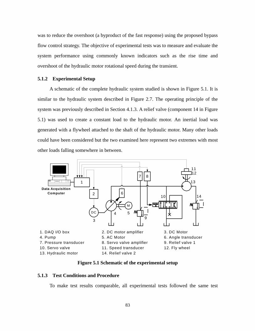
5.1.2 Experimental Setup
A schematic of the complete hydraulic system studied is shown in Figure 5.1. It is
similar to the hydraulic system described in Figure 2.7. The operating principle of the
system was previously described in Section 4.1.3. A relief valve (component 14 in Figure
5.1) was used to create a constant load to the hydraulic motor. An inertial load was
generated with a flywheel attached to the shaft of the hydraulic motor. Many other loads
could have been considered but the two examined here represent two extremes with most
other loads falling somewhere in between.
DC
M
1. DAQ I/O box 2. DC motor amplifier 3. DC Motor4. Pump 5. AC Motor 6. Angle transducer7. Pressure transducer 8. Servo valve amplifier 9. Relief valve 110. Servo valve 11. Speed transducer 12. Fly wheel13. Hydraulic motor 14. Relief valve 2
7
6Data Acquisition
Computer
1
2
3
4 59
13
14
11
10
812
Figure 5.1 Schematic of the experimental setup
5.1.3 Test Conditions and Procedure
To make test results comparable, all experimental tests followed the same test
84
conditions. They were as follows:
• The temperature of the fluid was kept at 25±1.5°C during each test.
• The pressure of the relief valve 1 (component 9 in Figure 5.1) was set to 20.7
MPa (for safety purposes).
• The rotational speed input signal was a step function with an initial value of
40 rad/s and a final desired value of 100 rad/s. It was common for all tests.
The step was initiated at 2 second to allow starting transients to die down.
• All tests were repeated three times to check the repeatability.
• All transducers were re-calibrated before each set of tests.
In order to evaluate the performance of the circuit, the rotational speed of the
hydraulic motor was measured at different loading conditions by changing the pressure
level and load type (fixed and inertial loads). A uniform measurement procedure was
adopted to make test results comparable. The main steps were as follows:
1) A step input signal was applied to the DC motor controller (without using the
bypass flow control), and the motor rotational speed measured.
2) Without changing test conditions, the same step input signal (desired value
100 rad/s) was applied to the DC motor controller and bypass valve controller
(using the bypass flow control algorithm) simultaneously, and the motor
rotational speed measured.
3) The backpressure on the hydraulic motor was increased by adjusting the load
relief valve from 0 MPa to 12.8 MPa in increments of 1.73 MPa.
5.2 Experimental Test with a Fixed (Constant) Load
For a positive displacement pump, such as the axial piston pump, flow is generated,
not pressure. The pump transfers the fluid at a controllable rate into the system which
encounters some resistance to the fluid flow (due to a load or line losses etc.). The
resistance from the piping, hoses, and fittings is quite small with proper component
85
selection. The largest part of the resistance to the fluid flow comes from the load itself.
According to system external constraints, the load can be a constant (such as that due to
gravity), resistive, capacitive, inertial, or some combination. Different kinds of loads have
different characteristics and have different effects on the system performance. This first
section will consider the performance of the bypass system under the conditions of a
constant resistive load. An inertial load is considered in the next section.
The characteristic of the resistive or constant resistive (hereafter referred as just
“constant”) load is that the load reaction on the output device always opposes the motion
of the hydraulic motor. In this test, a constant load was simply simulated by applying a
backpressure to the outlet of the hydraulic motor using a relief valve. Because of the
characteristics of a relief valve, the backpressure was not exactly constant but showed a
pressure override of 3% at 5 GPM. This was considered to be an acceptable variation.
5.2.1 Experimental Test Results
According to the test procedure described in Section 5.1.3, the rotational speed of
the hydraulic motor was measured at pressures varying from 0 MPa to 12 MPa. Figure 5.2
shows the dynamic responses of the hydraulic motor with a backpressure of 5.18 MPa.
It was observed that the rise time of the hydraulic motor rotational speed was about
34 ms. The rise time was the same for systems with and without bypass flow control since
the valve was closed during this time period. The overshoot was reduced significantly
when the bypass flow control system was used. The hydraulic motor rotational speed
reached its approximate steady state condition after transients have died out. However, the
motor rotational speed did experience an oscillation (defined in this thesis as a
non-uniform flow, pressure or rotational speed ripple, hence forth referred to as simply
“ripple”) about its steady state value as illustrated in Figure 5.2. The presence of the ripple
will be discussed in Section 5.2.3.
86
Figure 5.2 Dynamic responses of the hydraulic motor at a backpressure of 5.18 MPa
Figure 5.3 shows the dynamic performance of the hydraulic motor (in terms of its
rotational speed) at four particular pressure levels. All measured rotational speed signals
were filtered with a low pass filter. The cut-off frequency of the filter was 250 Hz. Figure
5.3 illustrates that the bypass flow control system was effective in reducing the overshoot
at both low and high pressure loads. The dashed lines are the motor rotational speed of the
system without the bypass control, and those curves with solid line represent those with
bypass control. It is observed that the rise time is reduced and the overshoot increased with
increasing backpressure. The bypass flow control was effective for all pressure levels.
For each test, the performance of the dynamic response was evaluated using
indicators such as the steady state value, ripple magnitude (RMS), rise time and percent
overshoot. The technical definitions of the specifications are given in Section 2.5. Their
87
values were calculated with a Matlab® program using the data measured during the
transient or steady state.
Figure 5.3 Dynamic responses of the hydraulic motor at 4 particular backpressures
Percent Overshoot
The primary purpose of using the bypass flow control was to remove the overshoot
during the transient and hence, the percent overshoot of the hydraulic motor rotational
speed was the main indicator in which the performance of the bypass flow control was
assessed.
Figure 5.4 shows the percent overshoot of the motor rotational speed with and
without the bypass flow control. Three test results and their average values are shown in
the same figure. It was observed that the bypass flow control system could remove about
half of the total overshoot.
88
0
10
20
30
40
50
60
70
80
90
0 2 4 6 8 10 12
Backpressure (MPa)
Perc
ent O
vers
hoot
of R
otat
iona
l Spe
edTest 1 without bypassTest 1 with bypassTest 2 without bypassTest 2 with bypassTest 3 without bypassTest 3 with bypassAverage without bypassAverage with bypass
Percent Overshoot without bypass flow control
Percent Overshoot with bypass flow control
Figure 5.4 Comparison of overshoot between systems with/without bypass control
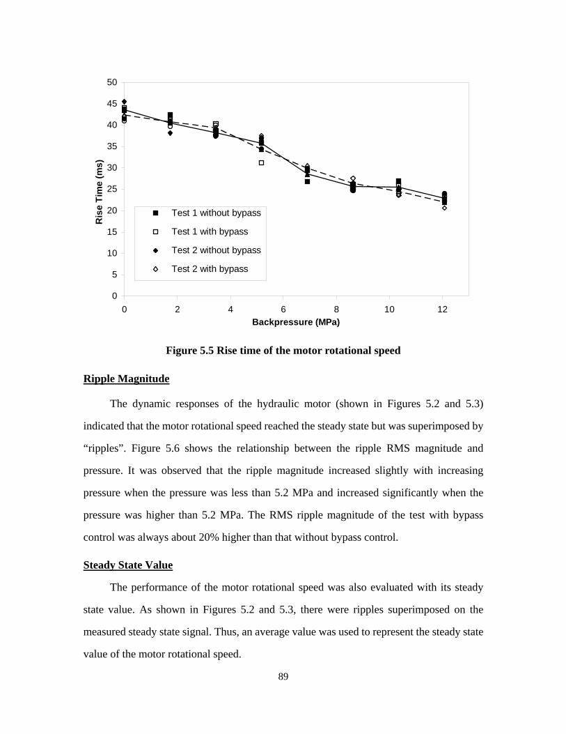
Rise Time
The main objective of this research was to improve the dynamic response of the
pump controlled system. The rise time was a main indicator for evaluating the rate of the
dynamic response. A smaller rise time represented a fast dynamic response. Figure 5.5
shows the rise time of the motor rotational speed with and without bypass flow control.
The average value of the rise time with bypass control is shown in the dash thick line, and
that without bypass control is shown in solid thick line. It was observed that the rise time
was between 20 and 45 ms and decreased with increasing pressure.
As mentioned above, the rise time of the motor rotational speed changed with the
pressure: large at low pressures and small at high pressures. This was a direct consequence
of the nonlinear DC motor controller. The smaller DC motor controller gains at low
pressures resulted in a slow (damped) response and large rise time, whereas the overshoot
increased with increasing pressures due to the larger controller gains.
89
0
5
10
15
20
25
30
35
40
45
50
0 2 4 6 8 10 12Backpressure (MPa)
Ris
e Ti
me
(ms)
Test 1 without bypass
Test 1 with bypass
Test 2 without bypass
Test 2 with bypass
Figure 5.5 Rise time of the motor rotational speed
Ripple Magnitude
The dynamic responses of the hydraulic motor (shown in Figures 5.2 and 5.3)
indicated that the motor rotational speed reached the steady state but was superimposed by
“ripples”. Figure 5.6 shows the relationship between the ripple RMS magnitude and
pressure. It was observed that the ripple magnitude increased slightly with increasing
pressure when the pressure was less than 5.2 MPa and increased significantly when the
pressure was higher than 5.2 MPa. The RMS ripple magnitude of the test with bypass
control was always about 20% higher than that without bypass control.
Steady State Value
The performance of the motor rotational speed was also evaluated with its steady
state value. As shown in Figures 5.2 and 5.3, there were ripples superimposed on the
measured steady state signal. Thus, an average value was used to represent the steady state
value of the motor rotational speed.
90
0
1
2
3
4
5
6
7
0 2 4 6 8 10 12Backpressure (MPa)
RM
S R
ippl
e M
agni
tude
(rad
/s)
Test 1 without bypassTest 1 with bypassTest 2 without bypassTest 2 with bypassTest 3 without bypassTest 3 with bypassAverage without bypassAverage with bypass
Average RMS ripple magnitudewithout bypass flow control
Average RMS ripple magnitudewith bypass flow control
Figure 5.6 RMS Ripple magnitude of the motor rotational speed
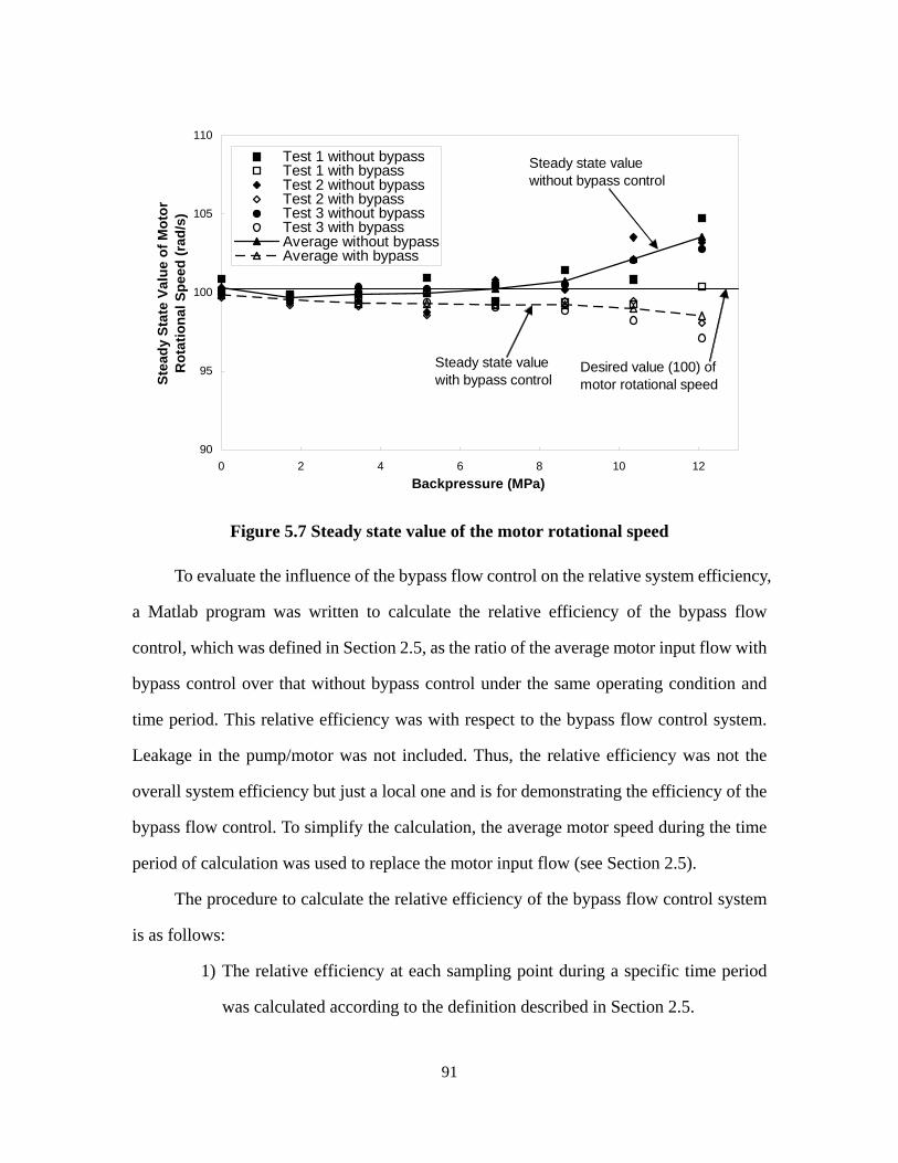
Figure 5.7 shows the average steady state value of the motor rotational speed as a
function of pressure. It was observed that the steady state values varied at 100±1 rad/s for
tests with and without bypass control when the pressure was less than 6.9 MPa. When the
pressure was higher than 6.9 MPa, the average steady state value increased with increasing
pressure for tests without bypass control. For tests with bypass control, the average steady
state value decreased slightly with increasing pressure and was always less than that
without bypass control.
5.2.2 Relative Efficiency of the Bypass Flow Control System
As proposed in Section 1.4, the objective of this study was to improve the
performance of an existing pump-controlled motor system without sacrificing its overall
high relative efficiency. The test results discussed above showed that the performance of
the pump controlled motor system was partly improved by using the bypass flow control
system in which the overshoot was reduced by about 50%. However, the bypass control
also had a negative effect on the relative system efficiency.
91
90
95
100
105
110
0 2 4 6 8 10 12Backpressure (MPa)
Stea
dy S
tate
Val
ue o
f Mot
orR
otat
iona
l Spe
ed (r
ad/s
)Test 1 without bypassTest 1 with bypassTest 2 without bypassTest 2 with bypassTest 3 without bypassTest 3 with bypassAverage without bypassAverage with bypass
Steady state valuewithout bypass control
Steady state valuewith bypass control
Desired value (100) of motor rotational speed
Figure 5.7 Steady state value of the motor rotational speed
To evaluate the influence of the bypass flow control on the relative system efficiency,
a Matlab program was written to calculate the relative efficiency of the bypass flow
control, which was defined in Section 2.5, as the ratio of the average motor input flow with
bypass control over that without bypass control under the same operating condition and
time period. This relative efficiency was with respect to the bypass flow control system.
Leakage in the pump/motor was not included. Thus, the relative efficiency was not the
overall system efficiency but just a local one and is for demonstrating the efficiency of the
bypass flow control. To simplify the calculation, the average motor speed during the time
period of calculation was used to replace the motor input flow (see Section 2.5).
The procedure to calculate the relative efficiency of the bypass flow control system
is as follows:
1) The relative efficiency at each sampling point during a specific time period
was calculated according to the definition described in Section 2.5.
92
2) The average relative efficiency was calculated by averaging the individual
relative efficiencies calculated at all sampling points over the whole time
period.
Figure 5.8 shows the relative efficiency of bypass flow control system in terms of
this ratio.
Figure 5.8 Relative efficiency of the bypass control system
Note: the step occurred at 2000 ms for all tests in this section.
The relative efficiency of the system with the bypass flow control was separately
calculated during the transient and steady state (after transient) periods. The transient
discussed in this case was considered as the time period started from the step point until
the transient died out. Since the transient time changed with loading conditions, it was
difficult to get a uniform transient time. On the other hand, the ripples also affected the
93
estimation of the transient time. Hence, a typical transient period of 200 ms was assumed
for all tests, during which most transient had died out. Figure 5.8(a) shows the relative
efficiency during the transient. It was observed that the relative efficiency of the bypass
control during the transient was 96% with a scatter of about ±1%. Figure 5.8(b) shows the
relative efficiency during the steady state, a time period of 1800 ms after the transient.
This figure shows that the relative efficiency decreased slightly from about 100% to 99%
when the backpressure increased from 0 MPa to 8.6 MPa and decreased quickly to 95%
when the pressure increased to 12 MPa. Figure 5.8(c) shows the average relative
efficiency during the whole time period (2000 ~ 4000 ms) including the transient and
steady state. The trend of the combined average relative efficiency was quite similar to the
trend of the steady state relative efficiency. The relative efficiency varied around 99%
when the pressure was less than 6.9 MPa, and decreased with increasing pressure.
All results shown in Figure 5.8 indicated that the relative efficiency of the bypass
flow control system was less than 100%. It varied between 99% and 95% depending on
loading conditions. This meant the bypass valve was not fully closed during the steady
state as expected. A small portion of the flow, which was approximately equal to 100%
minus the relative efficiency, was bypassed through the valve. The reason for this was due,
in part, to the motor rotational speed ripple which was fed back to the bypass valve
controller through the rotational speed transducer. In essence, the bypass flow control
system treated the rotational speed ripples as an overshoot. Because the valve was opened
during the ripple overshoot, the effect was to bias the steady state value to something
lower than that without bypass control.
5.2.3 Variations in the Rotational Speed Ripple: Discussion
Experimental results shown in the last section indicated that the rotational speed of
the hydraulic motor approach steady state in less than 100 ms. However, superimposed on
94
the measured rotational speed signal was a periodic and non-uniform disturbance signal
(ripple and noise) which did not diminish under steady state conditions. This section will
discuss the source of the noise and ripple.
A typical motor rotational speed signal is shown in Figure 5.9 (a). The steady state
value of the rotational speed (DC value) was 100 rad/s. It was observed that two kinds of
signals were superposed on the DC signal. One was in the form of non-periodic noise, and
the other one was a periodic, non-uniform ripple signal. The non-periodic noise signal,
which occasionally appeared in random “spurts”, was mainly due to the amplifier of the
DC motor (see the large spurts shown in Figure 5.9(a)). The DC motor amplifier used
pulse width modulation methods to amplify the electrical signal. It controlled the current
of the DC motor by varying the duty cycle of the output power under a fixed switching
frequency (22 kHz). A noise signal with this frequency was transmitted from the amplifier
to all electronic signals (such as rotational speed, swash plate angle and pressure
transducers) through the electrical ground. Since the sampling frequency was only 1000
Hz, the noise signal was occasionally sampled by the data acquisition system and appeared
randomly in the measured signals in the form of spurts. Many attempts were made to
prevent the noise from appearing into the sampling system without compromising the
information from the base signal but without success.
The most significant effect on the rotational speed was the non-uniform (magnitude
wise) but periodic ripple. The ripple was, in fact, composed of several frequencies. To find
out what the frequency spectrum of the non–uniform ripple was, an analytical method
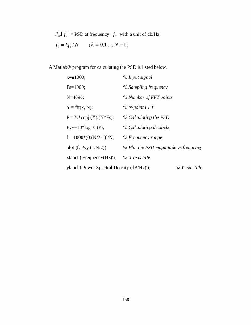
called the power spectral density (PSD) (see Appendix E) was used to process the noise
signal. The noise signal used for the PSD analysis was not filtered. Figure 5.9(b) shows the
PSD result of the motor signal (shown in Figure 5.9(a)).
95
Figure 5.9 A typical motor rotational speed signal and its power spectral density
It was observed that the energy contained in the signal was mainly concentrated at 6
frequencies which could be directly correlated with physical conditions or component
behavior. They were:
• f1=16 Hz, the rotational speed of the hydraulic motor,
• f2=30 Hz, the rotational speed of the pump and pump driver (AC motor),
• f3=32 Hz, the second harmonic of the hydraulic motor rotational speed,
• f4=64 Hz, the forth harmonic of the hydraulic motor rotational speed,
• f5=270 Hz, the rotational speed of pump pistons, equal to the product of the
pump rotational speed and the number of pistons (9), and
• f6=352 Hz, the rotational speed of the rotational speed transducer commutators,
equal to the product of the hydraulic motor rotational speed and commutator
number (22).
96
As mentioned, these six frequencies were highly correlated to physical components
in the system. The PSD result also showed some frequency components which had a
smaller power. These frequencies corresponded to higher harmonics of the pump and
motor rotational speed, and other characteristics of the system. They were, however,
comparatively small in power than the six mentioned above.
The PSD as a function of pressure for the six main frequencies are shown in Figure
5.10. The actual frequency values were only approximately constant, and changed slightly
with loading conditions. For example, the frequency of the pump rotation decreased from
29.8 Hz to 28.8 Hz when the pressure increased from 0 to 12.1 MPa. Test results for the
system with the bypass flow control are also shown in the same figure for comparison.
Figure 5.10 PSD magnitudes as the function of the pressure
The results from Figure 5.10 indicated that the PSD magnitudes increased with
increasing pressure at most of the frequencies (except at the frequency of 352 Hz). This
97
pressure dependency was consistent in both the PSD magnitude and the ripple RMS
magnitude results. The test results also showed the rotational speed ripple was mainly a
consequence of the pump basic rotational frequency for the system with and without the
bypass control. One such example can be observed in Figure 5.2, in which the underlying
ripple frequencies (again, with and without bypass control) were both about 30 Hz, the
frequency of the pump rotation.
Another observation that can be made from Figure 5.10 is that the PSD magnitudes
for the system with bypass control are larger than those in the system without bypass
control at most pressure levels.
An interesting situation occurs at pressures higher than 10 MPa. The ripples for the
system without the bypass flow control were mainly a consequence of the motor rotational
frequency (as opposed to the pump rotational frequency) - see the top left figure in Figure
5.10. The motor rotation frequency PSD magnitude increased significantly when the
system operated at higher pressures. This result was consistent with the RMS ripple
magnitude at pressures greater than 12 MPa (see Figure 5.6).
The dependency of the ripple base frequency on the rotational speed of the pump
and at higher pressures, the motor, was not expected. Normally, one would expect the
ripple to be dominated by the frequency associated with the nine pistons for both the pump
and motor. This was not the case and does indicate that the PSD was picking up some
disturbance introduced by some fault or wear in the pump and motor. Both units were off
the shelf components and have been well used. As mentioned, these disturbances were
highly dependent on the system load and hence pressure. This dependency on the pressure
could be attributed, in part, to the nonlinear gains on the DC motor controller which would
tend to amplify any perturbations in pressure due to the motor, for example. The point to
be made here is that the presence of the ripple was a consequence of the pump and motor
dynamics and was not introduced by the bypass control algorithm. The bypass controller
98
did, however, try to compensate for pump ripple as discussed above.
Compared to the pump and motor rotation, pump pistons and transducer
commutators had comparably smaller effects on the ripple RMS value. At the frequencies
of these components, there were no significant differences between the systems with and
without bypass flow control.
5.3 Experimental Test with a Inertial and Constant Resistive Load
The controllers designed for the DC motor and bypass control valve were based on a
constant resistive load. The results for a constant resistive load were consistent with that
predicted by theory. This section will present the results of the DC motor controlled pump
and bypass flow control system in the presence of an inertial load and a constant load. A
flywheel was attached to the motor shaft to simulate the inertia load. The inertial load had
a different characteristic from other load types due to its moment of inertia. Usually, a
system with an inertial load will demonstrate a large overshoot and undershoot during the
transient due to the presence of the inertia of both the fluid (due to the pump) and load.
Figure 5.11 shows the dynamic response of the hydraulic motor with an inertial load.
A fixed backpressure was set to 3.45 MPa. It was observed that the system without using
the bypass control exhibited a limit cycle oscillation. The system with bypass control did
reach steady state but only with a long settling time and large undershoot. The test results
measured at other pressures also exhibited a similar performance.
It was apparent that the limit cycle oscillation was not caused by using the bypass
flow control since the system with the bypass control demonstrated a stable performance.
It was believed that the limit cycle oscillation might be caused by the DC motor since the
DC motor controller was heavily dependent on the load pressure. In the constant load, the
DC motor did have an affect on the amplitude of the overshoot due to the controller gain's
dependency on pressure. To see if this effect was present in the inertial load which showed
extreme variations in pressure, a new DC motor controller was designed for the same
99
backpressure with the inertial load applied. The bypass flow control system was not
included in the design and hence the control algorithm remained unchanged. A similar
procedure, which was used to design the original DC motor controller, was followed.
Figure 5.11 Dynamic response of the hydraulic motor with an inertial load
First, the proportional gain of the DC motor controller was increased until the
hydraulic system exhibited a limit cycle oscillation (shown in Figure 5.12(a)).
It was observed that the pump swashplate angle experienced a limit cycle oscillation
of 30 Hz. However, the hydraulic motor limit cycle frequency was at some value other
than this. A PSD analysis indicated two dominant frequencies present in the motor
rotational speed signal. The spread of frequencies about 30 Hz was quite narrow but
showed a larger power in general. The second dominant frequency was at 11 Hz but
showed a wide band and slightly smaller PSD magnitude.
100
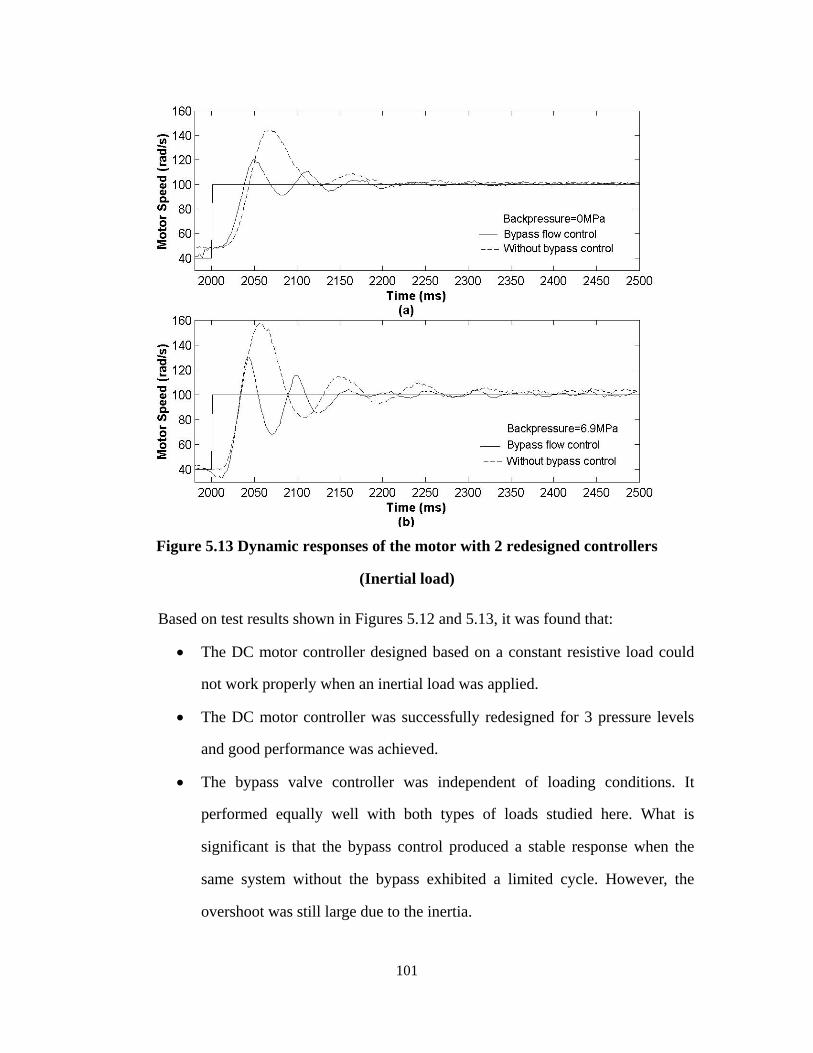
Figure 5.12 Redesign of the DC motor controller with the inertial load
As a first step, the 30 Hz was used as a basis for the design of the controller using
Ziegler-Nichols tuning PID rules. However, the hydraulic motor exhibited a clear
oscillation at the frequency of 11 Hz (shown in Figure 5.12(b)) when the controller was
applied to the DC motor.
The final DC motor controller was thus designed based on a frequency of 11 Hz.
Test results for the new designed controller are shown in Figure 5.12(c). It is observed that
the new DC motor controller shows a better performance than the previous controller for
the inertial load.
Using the same procedure as above two more controllers were designed at
backpressures of 0 MPa and 6.9 MPa. Test results of these two controllers are shown in
Figure 5.13.
101
Figure 5.13 Dynamic responses of the motor with 2 redesigned controllers
(Inertial load)
Based on test results shown in Figures 5.12 and 5.13, it was found that:
• The DC motor controller designed based on a constant resistive load could
not work properly when an inertial load was applied.
• The DC motor controller was successfully redesigned for 3 pressure levels
and good performance was achieved.
• The bypass valve controller was independent of loading conditions. It
performed equally well with both types of loads studied here. What is
significant is that the bypass control produced a stable response when the
same system without the bypass exhibited a limited cycle. However, the
overshoot was still large due to the inertia.
102
For the inertial load, a DC motor controller could be redesigned with an acceptable
performance. At pressures higher than 12 MPa, the system performance was not
acceptable and could not be improved by controller redesign. For pressures less than 12
MPa, a pressure dependent nonlinear controller could be designed for inertial loads.
In summary, the DC motor controller was dependent on both the system pressure,
and load type. A nonlinear controller could be designed to adapt any load conditions.
5.4 Summary of the Experimental Tests
The concept of the bypass flow control was experimentally evaluated in the previous
sections. Test results showed good performances of the DC motor controlled pump and
bypass flow control system. The following presents a summary of the experimental tests.
Summary for the system without using the bypass flow control
1. The rise time of the hydraulic motor, which was directly controlled by the
pump, was between 20 to 50 ms, depending on loading conditions.
2. The overshoot was more than 30% for a constant resistive load and inertia
load.
3. The hydraulic motor rotational speed reached steady state in 100 ms for the
constant load, and in about 250 ms for the inertial load.
4. A non-uniform ripple was superimposed on hydraulic motor’s steady state
rotational speed. The RMS magnitude of the ripple increased with increasing
pressure.
Summary for the system using the bypass flow control system
1. The relative efficiency of the bypass flow control system varied from 99% to
95% depending on loading conditions. This meant that about 1% to 5% flow
was bypassed through the bypass valve during the transient and steady state
due to the overshoot and ripples. For a pump/motor that does not demonstrate
103
significant flow ripple of the magnitude experienced in this study, the relative
efficiency would be the same as the pump/motor system without bypass.
2. The bypass flow control system effectively reduced the overshoot of the
motor rotational speed by about 50%.
3. The rise time was not affected by using the bypass flow control.
4. The steady state error was slightly larger than the system without using the
bypass flow control due to the inherent bias created by the ripples at most of
the pressure levels.
5. The valve was not fully closed during the steady state as expected due to the
presence of ripple. Hence, a very small portion of the flow was bypassed to
the tank across the bypass valve. This would have an effect on reducing the
efficiency but the reduction was considered to be small.
104
Chapter 6
Conclusions and Recommendations
6.1 General
The objective of this study was to develop a hydraulic circuit with good dynamic
performance and high efficiency. This was, in part, realized by improving the dynamic
performance of an energy efficient pump-controlled system. The pump-controlled system
has a very high relative system efficiency due to the minimization of the power loss
between the pump and actuator. To improve the dynamic performance of the pump, a DC
motor was designed to directly control the pump swashplate. In order to facilitate the
design of a DC motor controller with good performance, the pump and DC motor were
mathematically modeled. Using this model, combined with some experimental results, a
nonlinear PID controller was designed for the DC motor. The gains of the controller were
designed to be a function of the pressure. By means of this nonlinear DC motor controller,
the pump could operate in a relative stable manner without limit cycle oscillation at any
pressure levels and at most swashplate angles (only swashplate angles between 3˚ and 14˚
were tested). Test results showed that the DC motor-controlled pump did indeed,
demonstrate a fast dynamic response. The rise time of the pump swashplate angle was less
than 40 ms over the whole range of pressures examined independent of the swashplate
final angle. A fast dynamic response speed could be achieved with a rise time of less than
17 ms if the pump pressure increased to 6.9 MPa.
As the dynamic response speed of the pump was increased, the overshoot of the
hydraulic motor’s response also increased (between 35% and 70%). To reduce the
overshoot, a bypass flow control system was designed to bypass part of the pump flow
during the transient. Before designing the controller for the bypass valve, the complete
105
system model (including the bypass servo valve and hydraulic motor) was established.
Since the bypass flow control system could not respond to a negative signal, a PID
controller with a resetable integral gain was designed for the bypass valve based on the
model simulation. “Proof of concept” of bypass flow control was established using a
Matlab/Simulink® program. The simulation results showed that the bypass flow control
could effectively reduce the overshoot of the motor rotational speed.
The dynamic performance of the pump controlled system and the concept of the
bypass flow control were evaluated through a series of experimental tests. Two load types
(constant resistive and inertial) were applied to the hydraulic motor. Test results showed
that the experimental pump-controlled system indeed, demonstrated a very fast dynamic
response. However, the DC motor controller designed for a constant load did not work in a
stable fashion under inertial load conditions. The bypass control system was able to
provide a stable response but the settling time was large. By redesigning the DC motor
controller, the hydraulic motor could reach the steady state without any limit cycle
oscillations. The bypass flow control system worked effectively for all controllers
regardless of the loading conditions.
6.2 Conclusions
As the result of this study, the following conclusions are made.
1. It was concluded that the dynamic response of the pump was improved by
using the DC motor control approach. The pump swashplate was directly
controlled by a DC motor instead of using the more commonly used
hydraulically actuated control approach. Because of the fast dynamic
response of the DC motor, the DC motor controlled pump exhibited a rise
time of 15 to 35 ms depending on the pump pressure.
2. The bypass flow control system was effective in removing the overshoot.
Under different loading conditions, the bypass flow control could reduce the
106
overshoot of the hydraulic motor rotational speed by about 50%.
3. The relative efficiency of the circuit was almost the same as the
pump-controlled system. It was affected slightly (in a negative sense) by
using the bypass flow control. The bypass valve was not completely closed as
expected during the steady state due to the rotational speed ripples. The
relative efficiency of the circuit with the bypass flow control system was 1%
to 5% lower for the particular pump-controlled system that was used in this
study. If the pump/motor did not demonstrate the rotational speed ripples, the
relative efficiency would be the same as the pump/motor system without
bypass.
6.3 Recommendations
Some considerations that should be investigated in the future work are:
1. The bypass flow control system could effectively remove the overshoot, but
not the undershoot. A "flow supplement" system might be considered as a
means of providing the extra flow to the system when the motor exhibits an
undershoot.
2. The rotational speed ripple was caused mainly by the rotation of the pump
and motor. However, it was not clear how the pump and motor rotation
affected the magnitude of the rotational speed ripple. More analysis and
experimental tests needs to be done to solve this problem. The magnitude of
the rotational speed ripples could be reduced with a new design approach.
3. The DC motor was not as stiff as its hydraulic counterpart. The load heavily
affected its performance. Also, the DC motor controller was dependent on
loading conditions. This problem could be solved by designing a DC motor
controller that could adapt to different loading conditions. To do so, a wide
range of loading conditions (such as the pressure, flow rate and load types)
107
should be investigated during the design.
4. The system stability may be improved by using system identification and
pole-zero placement strategies.
108
References
1. Backe, W., 1991, “Electrohydraulic loadsensing”, Proceedings of the International
Off-Highway and Powerplant Congress and Expostion, Sep 9-12, Milwaukee, USA.
2. Backe, W., 1993, “Recent Research Projects in Hydraulics”, Proceedings of the
Second JHPS International Symposium on Fluid Power, September 6-9, Tokyo,
Japan, pp.3-27
3. Backe, W. and Kogl, C., 1993, “Secondary controlled motors in speed and torque
control”, Proceedings of the Second JHPS International Symposium on Fluid Power,
September 6-9, Tokyo, Japan, pp.241-248.
4. Burgt, J., 1993, "A new approach to saving energy in cyclic loaded hydraulic
systems: learning hydraulic systems", Proceedings of the 3rd International
Conference on Fluid Power Transmission and Control, Hangzhou, China,
pp.123-130.
5. Cundiff, J. S., 2002, "Fluid Power Circuits and Controls: Fundamentals and
Applications", CRC Press, Roca Raton.
6. Habibi, S., 2001, "Lecture notes: Control System I", Department of Mechanical
Engineering, University of Saskatchewan.
7. Käppi, K., 2000, "Modeling and Simulation Utilized in Research and Development
of Mobile Hydraulics", Proceedings of the 1st FPNI-PhD Symposium, Hamburg,
Germany, pp.353-361.
8. Kavanagh, G. P., 1987, "The Dynamic modeling of an Axial Piston Hydraulic
Pump", M.Sc Thesis, Department of Mechanical Engineering, University of
Saskatchewan.
9. Lantto, B., Krus, P. and Palmberg, J., 1991, “Interaction between loads in
load-sensing systems”, Proceedings of the 2nd Tampere International Conference on
109
Fluid Power, March 19-21, Tampere, Finland.
10. Li, Z., Ge, Y. and Cheng, X., 1998, "Hydraulic Components and Systems" (in
Chinese), China Mechanical Industry Press, pp2-3.
11. Liang, X., Virvalo, T. and Linjama, M., 1999, “The Influence of Control valves on
the efficiency of a Hydraulic Crane”, Proceedings of the 6th Scandinavian
International Conference on Fluid Power, May 26-28, Tampere, Finland,
pp.381-394.
12. Liang, X. and Virvalo, T., 2001 (1), “What's wrong with energy utilization in
hydraulic cranes”, Proceedings of the 5th International Conference on Fluid Power
Transmission and Control, April 3-5, Hangzhou, China, pp.419-424
13. Liang, X. and Virvalo, T., 2001 (2), “Energy reutilization and balance analysis in a
hydraulic crane”, Proceedings of the 5th International Conference on Fluid Power
Transmission and Control, Hangzhou, China, pp.306-310.
14. Luomaranta, M., 1999, “A Stable electro-hydraulic load sensing system based on a
microcontroller”, Proceedings of the Sixth Scandinavian International Conference
on Fluid Power, May 26-28, Tampere, Finland, pp.419-432.
15. Mack, P., 1985, "Feasibility Study of the Use of a Microcomputer to Control the
steady state Operating Characteristics of a Variable Displacement Hydraulic Pump”,
Master’s Thesis, Department of Mechanical Engineering, University of
Saskatchewan, University of Saskatchewan.
16. Malsen, R., Achten, P. and Vael, G. 2002, “Design of Dynamic and Efficient
Hydraulic Systems around a Simple Hydraulic Grid”, Proceedings of the SAE
Off-Highway Congress, March, Las Vegas, USA.
17. Mansouri, G., Misovec, K., Johnson, B., Babbitt, G. and Sturman, O., 2001,
“Variable flow supply using switched-mode control of a fixed-displacement pump”,
Proceedings of the Seventh Scandinavian International Conference on Fluid Power,
110
May 30-June, Linkoping, Sweden, pp.361-376.
18. Martin, M., 1992, "Load Simulator Using Hydraulics”, Master’s Thesis, Department
of Mechanical Engineering, University of Saskatchewan, University of
Saskatchewan.
19. Merritt, H., 1967, "Hydraulic Control Systems", John Wiley & Sons, Inc., New York,
pp.152-157.
20. Nakano, K. and Tanaka, Y., 1988, “Energy-saving type electro-hydraulic servo
system”, The Journal of Fluid Control, v 18, n 3, p 35-51.
21. Post, W. and Druten, R., 2001, “The design of energy-efficient power transmissions:
Learning hydraulic systems and zero-inertia power transmission”, Bath Workshop
on Power Transmission and Motion Control, Professional Engineering Publishing
Ltd., London, pp.245-258.
22. Rahmfeld, R., 2000, “Development and Control of Energy Saving Hydraulic Servo
Drives”, Proceedings of the 1st FPNI-PhD Symposium, Hamburg, Germany,
pp.167-180.
23. Rahmfeld, R. and Ivantysynova, M., 2001, “Displacement controlled linear actuator
with differential cylinder –a way to save primary energy in mobile machines”,
Proceedings of the 5th International Conference on Fluid Power Transmission and
Control, Hangzhou, China, pp.296-301.
24. Ramirez, R. W., 1985, "The FFT Fundamentals and Concepts", Prentice-Hall, Inc.,
New York.
25. Tanaka, Y., Nakano, K. and Yamamoto, N., 1989, “Energy–Saving Hydraulic Power
Source Using Inverter-Motor Drive”, Proceedings of the First JHPS International
Symposium on Fluid Power, Tokyo, Japan.
26. Tikkanen, S., Herranen, M., Lammila, M. and Vilenius, M., 2001, “Performance of
Dual Hydraulic Free Piston Engine”, Proceedings of the Seventh Scandinavian
111
International Conference on Fluid Power, May 30-June 1, Linkoping, Sweden,
pp.133-150.
27. Vael, G. E. M., Achten, P. A. J., 1998, “The Innas Fork Lift Truck -Working under
constant pressure”, Proceedings of the first International Fluid Power Conference,
Part 1, M Verlag Mainz, Aachen.
28. Vael, G. E. M., Achten, P. A. J., Fu, Z., 2000, “The Innas Hydraulic Transformer:
The key to the hydrostatic Common Pressure Rail”, SAE 2000 Transactions Journal
of Commercial Vehicles, Vol. 100, Section 2.
29. Wendel, G., 2000, “Regenerative Hydraulic Systems For Increased Efficiency”,
Proceedings of the 47th National Conference on Fluid Power, April 4-6, Chicago,
USA, pp.199-206.
30. Wendel, G., 2002, “Hydraulic System Configurations for Improved Efficiency”,
Proceedings of the 49th National Conference on Fluid Power, March 19-21, Las
Vegas, Nevada, USA, pp.567-573.
31. Wu, D., 2003, " Modeling and Experimental Evaluation of a Load-Sensing and
Pressure Compensated Hydraulic System”, Ph.D Thesis, Department of Mechanical
Engineering, University of Saskatchewan.
32. Yao, D., 1997, "Research on a Direct Pressure Sensing Relief Valve ", M.Sc Thesis,
Department of Mechanical Engineering, University of Saskatchewan.
33. You, Z., 1989, "A Study on Interactions between Fluid Power Components", M.Sc
Thesis, Department of Mechanical Engineering, University of Saskatchewan.
34. Ziegler, J. G. and N. B. Nichols, 1942, "Optimum Settings for Automatic
Controllers", ASME Trans. 64 (1942), pp. 759-68.
35. “760 Series Servovalve”, Moog Inc., East Aurora, New York
36. “HT-High Torque, Direct Drive Series”, Emoteq Inc., Tulsa, Oklahoma
112
Appendix A
Calibration of the Measurement System
The measurement system shown in Figure A.1 consists of transducers, a data
acquisition system (DAQ) and amplifiers. System variables such as swashplate angle,
pressure and rotational speed are converted to voltage signals by the transducers and
collected by the computer through the DAQ. Output control signals from the computer are
amplified by the external amplifiers. I/O
Connector B
lock
Angular positiontransducer
Pressure transducer
Rotational speedtransducer
Flow rate transducer
Other transducer
Power amplifier
Bypass valvecontroller
Ribbon Cable
Swashplateangle
System pressure
Hydraulic motorrotational speed
Pump flow rate
Current, force
DC motor
Servo valve
Dataacqusition
board
Figure A.1 Measurement system
As a first step, the calibration of all transducers was completed before taking any
online measurements and control action to avoid measurements containing very large
offset, gain and linearity errors. This section will discuss the calibration of all transducers
and amplifiers used in the research.
113
A.1 Calibration of the Data Acquisition System
The DAQ includes a data acquisition board (NI PCI-6035E ) and an I/O connector
block. They are connected by a “ribbon cable”. The DAQ has 16 single-ended (eight
differential) analog input channels and 2 single-ended analog output channels, and has a
sampling frequency of 200 kHz. The resolution for the analog input (output) is 16 (12)
bits.
The DAQ can measure and condition the input signals which are stationary but
cannot compensate for time varying effects.
A.1.1 Calibration of analog input channels
In the calibration procedure, voltages are applied to the analog input and the input
voltage from the DAQ via the computer recorded. Preliminary results indicated that a DC
bias and a non-unity gain existed in the DAQ. The system gain was reset to achieve a unity
gain as shown in Figure A.2. In this figure, as in subsequent ones, the “error” is defined as
the difference between the measured output voltage (after adjustment) and a “best fit” line
which constitutes the “calibration equation”.
Calibration equationy = 1.0011x + 0.0017
-10
-5
0
5
10
-10 -5 0 5 10Applied Input Signal (V)
Mea
sure
d In
put S
igna
l (V)
-0.04
-0.02
0
0.02
0.04
Cal
ibra
tion
Erro
r (V)
Measured input signalCalibration error
Figure A.2 Calibration of analog input
114
The scatter of measured data with respect to the calibration best fit line falls within a
region of ±0.015 V (0.15% full scale). It was observed that after the adjustment to the
DAQ, the calibration best fit line was the same for all channels. In addition, tests were
repeatable with no visual difference.
A.1.2 Calibration of analog output channels
The calibration procedure of the DAQ analog output was as follows: Voltages were
generated by the computer and directed through the DAQ to each analog output channel.
The output voltages were measured at the terminal end of the connector block using a
highly accurate multimeter (Fluke 37, 0.1% full scale).
Similar to the input, a bias and a non-unity gain were observed. The DAQ was
adjusted and the calibration procedure repeated. The results are shown in Figure A.3 along
with the error. It is noted that a maximum error of 0.008 V (0.08% full scale) was observed.
The test was repeated for each channel and the same calibration equation occurred. The
test was highly repeatable with no visual difference in the results.
Calibration equationy = 0.9956x + 0.0214
-10
-5
0
5
10
-10 -5 0 5 10Demanded Output (V)
Mea
sure
d O
utpu
t Sig
nal (
V)
-0.02
-0.01
0
0.01
0.02
Cal
ibra
tion
Erro
r (V
)
Meadured output signalCalibration error
Figure A.3 Calibration of analog output
115
A.2 Calibration of the Angular Position Transducer
A Rotary Variable Inductance Transducer (RVIT, model R60D) was used to measure
the angle of the swashplate. The RVIT incorporates a set of printed circuit coils and a
conductive spoiler. During operation, the conductive spoiler rotates with the transducer
shaft, altering the magnetic field generated by the printed circuit coils. The resulting
imbalance is converted to a linear DC voltage output that is directly proportional to the
angle of the rotor shaft. The output range of the RVIT is ±60º.
To calibrate the RVIT, the angle of the shaft must be precisely measured. This was
done by converting the angular displacement to a linear displacement. A cylinder with a
diameter of 19 mm was coupled to the rotor of the transducer. The conversion to linear
displacement was achieved by connecting a thin wire wound on the cylinder to a linear
variable differential transducer (LVDT). A plot of the output voltage from the RVIT vs the
measurement source voltage is shown in Figure A.4. The error or deviation from a straight
best fit line is also shown.
Calibration equationy = 0.125x - 0.5991
-10
-5
0
5
10
-80 -60 -40 -20 0 20 40 60 80Angle (Degree)
Mea
sure
d O
utpu
t Vol
tage
(V)
-0.3
-0.2
-0.1
0
0.1
0.2
0.3
Cal
iobr
atio
n Er
ror (
V)
Measured output voltageCalibration error
Figure A.4 Calibration of angular position transducer
116
Most of the error lies within a range of ±0.125 V which corresponds to an angle of
±1º. The actual angular displacement of the pump is 20º. It is observed that on an absolute
scale, the range of 0~20º show a significant error variation. However, from 20~45º, the
error variation is small (less than ±0.02 V), Thus the angular RVIT was adjusted in the
20~45º range to match the displacement of the swashplate 0~20º.
A.3 Calibration of the Pressure Transducer
The pressure transducer (Sensotec model Z/6415-01ZG), which was used to
measure the pressure at the pump outlet, provides an output voltage directly proportional
to the applied pressure. The pressure transducer senses the pressure through a silicon type
pressure sensor diaphragm with strain resistors (a 4-arm active Wheatstone bridge)
combined with a signal conditioning circuit. The excitation voltage was 10 V DC
(regulated). The output signal range depends on the excitation voltage. The maximum
output range is 0 V~5.5 V DC.
The pressure transducer was calibrated with a twin seal pressure test dead weight
tester (Type 5525). Selected weights (representing system pressures) were applied to the
test unit and the related transducer output voltages measured. The output voltage as a
function of calibrated pressure is shown in Figure A.5. The calibration errors all fall in a
range of ±0.05 V (0.5% full scale).
A.4 Calibration of the Tachometer
A tachometer (Kearfott CM09608007) is a small generator whose rotator is
connected to the hydraulic motor shaft. The tachometer generates an output voltage
which is proportional to the rotational speed. The rotational speed of the hydraulic motor
was measured using a laser light source and the output voltage recorded by a multimeter.
The tachometer speed versus output voltage is shown in Figure A.6. The scatter of
the error falls within a range of ±0.045 V (0.7% full scale). It is noted that the error