J. Stefan Institute, Ljubljana, Slovenia Report DP-8955 Improving PID Controller Disturbance Rejection by Means of Magnitude Optimum Damir Vrančić and Satja Lumbar * * Faculty of Electrical Engineering, University of Ljubljana May, 2004
Transcript
J. Stefan Institute, Ljubljana, Slovenia
Report DP-8955
Improving PID Controller Disturbance Rejection by Means of Magnitude Optimum
Damir Vrančić and Satja Lumbar*
*Faculty of Electrical Engineering, University of Ljubljana
Appendix A. Comparison of disturbance-rejection properties of original MO and DRMO method for 63 process models ...................................................................... 18
Appendix B. List of Matlab and Simulink files used: ....................................................................... 91
3
4
1. Introduction
Most of the PID tuning methods available so far concentrate on improving tracking performance of the closed-loop.
One of such tuning methods is the magnitude optimum (hereafter “MO”) method [1,8,10,11,15,16,17], which results in a relatively fast and non-oscillatory system closed-loop response. The MO method is originally used for achieving superior reference tracking. On the other hand, by using the MO method, the process poles could be cancelled by the controller zeros. This may lead to poor attenuation of load disturbances if the cancelled poles are excited by disturbances and if they are slow compared to the dominant closed-loop poles [1]. Poorer disturbance rejection performance can be observed when controlling low-order processes. This is one of the most serious drawbacks of the MO method. In process control, disturbance rejection is usually more important than superior tracking [1,12].
Recently, a modified method for tuning parameters of PI controllers, based on the magnitude optimum method, has been developed. Namely, the original magnitude optimum (MO) has been adjusted for improving disturbance rejection by using the so-called disturbance-rejection MO (DRMO) method [18]. The results were encouraging, since disturbance rejection performance has been greatly improved, especially for lower-order processes.
Modification of the magnitude optimum method is not limited only to the PI controllers. The aim of this report is to show how the modification can be applied to PID controllers. However, since the structure of the PID controller is more complex, the calculation of the PID controller parameters cannot be performed analytically as is the case for the PI controller. Therefore, controller parameters should be calculated by numerical methods.
DRMO method for PI and PID controllers is compared to original MO method on 63 process models.
The report is set out as follows. Section 2 describes the original magnitude optimum tuning method for the PI and the PID controllers. Section 3 provides the theoretical background of disturbance rejection magnitude optimum method for the PI and the PID controller. Conclusions are given in section 5. Appendix shows the matlab files, which were used for the calculation of PI/PID controller parameters and the closed-loop simulation.
5
2. The original MO method
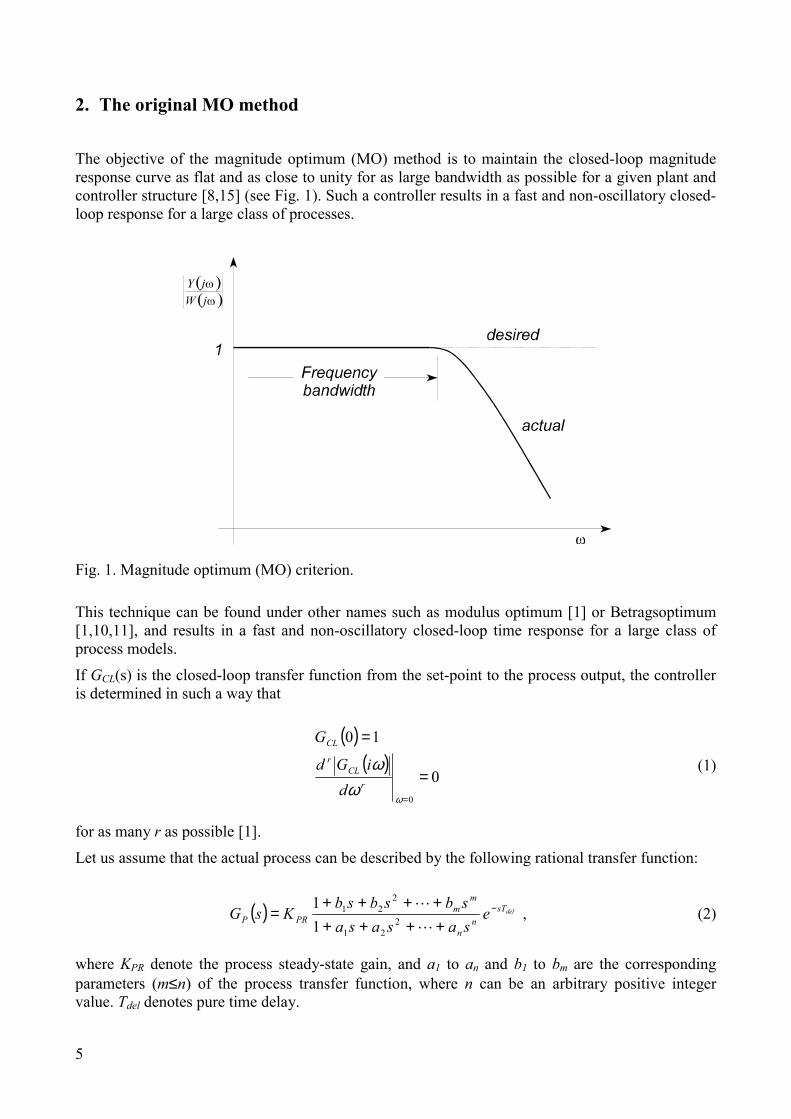
The objective of the magnitude optimum (MO) method is to maintain the closed-loop magnitude response curve as flat and as close to unity for as large bandwidth as possible for a given plant and controller structure [8,15] (see Fig. 1). Such a controller results in a fast and non-oscillatory closed-loop response for a large class of processes.
Fig. 1. Magnitude optimum (MO) criterion.
This technique can be found under other names such as modulus optimum [1] or Betragsoptimum [1,10,11], and results in a fast and non-oscillatory closed-loop time response for a large class of process models.
If GCL(s) is the closed-loop transfer function from the set-point to the process output, the controller is determined in such a way that
( )( )
0
10
0
=
=
=ωω
ωr
CLr
CL
diGd
G
(1)
for as many r as possible [1].
Let us assume that the actual process can be described by the following rational transfer function:
( ) delsTn
n
mm
PRP esasasasbsbsb
KsG −
++++++++
=L
L2
21
221
11
, (2)
where KPR denote the process steady-state gain, and a1 to an and b1 to bm are the corresponding parameters (m≤n) of the process transfer function, where n can be an arbitrary positive integer value. Tdel denotes pure time delay.
6
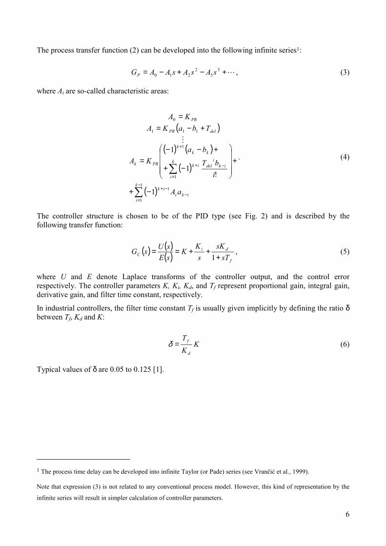
The process transfer function (2) can be developed into the following infinite series1:
L+−+−= 33
2210 sAsAsAAGP , (3)
where Ai are so-called characteristic areas:
( )
( ) ( )
( )
( ) iki
k
i
ik
iki
delk
i
ik
kkk
PRk
delPR
PR
aA
ibT
baKA
TbaKAKA
−
−
=
−+
−
=
+
+
∑
∑
−+
+
−+
+−−=
+−==
1
1
1
1
1
111
0
1
!1
1M
. (4)
The controller structure is chosen to be of the PID type (see Fig. 2) and is described by the following transfer function:
( ) ( )( ) f
diC sT
sKs
KK
sEsUsG
+++==
1, (5)
where U and E denote Laplace transforms of the controller output, and the control error respectively. The controller parameters K, Ki, Kd, and Tf represent proportional gain, integral gain, derivative gain, and filter time constant, respectively.
In industrial controllers, the filter time constant Tf is usually given implicitly by defining the ratio δ between Tf, Kd and K:
KKT
d
f=δ (6)
Typical values of δ are 0.05 to 0.125 [1].
1 The process time delay can be developed into infinite Taylor (or Pade) series (see Vrančić et al., 1999).
Note that expression (3) is not related to any conventional process model. However, this kind of representation by the
infinite series will result in simpler calculation of controller parameters.
7
PID+ _
w
d
y+
+ Processe u
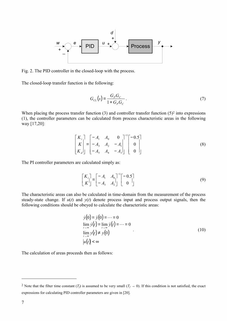
Fig. 2. The PID controller in the closed-loop with the process.
The closed-loop transfer function is the following:
( )CP
CPCL GG
GGsG
+=
1. (7)
When placing the process transfer function (3) and controller transfer function (5)2 into expressions (1), the controller parameters can be calculated from process characteristic areas in the following way [17,20]:
−
−−−−
−=
−
00
5.00 1
345
123
01
AAAAAA
AA
KKK
d
i
(8)
The PI controller parameters are calculated simply as:
−
−−
=
−
05.01
23
01
AAAA
KKi (9)
The characteristic areas can also be calculated in time-domain from the measurement of the process steady-state change. If u(t) and y(t) denote process input and process output signals, then the following conditions should be obeyed to calculate the characteristic areas:
( ) ( )( ) ( )( ) ( )
( ) ∞<
≠
======
∞→
∞→∞→
tu
yty
tytyyy
t
tt
0lim
0limlim000L&&&
L&&&
. (10)
The calculation of areas proceeds then as follows:
2 Note that the filter time constant (Tf) is assumed to be very small (Tf → 0). If this condition is not satisfied, the exact
expressions for calculating PID controller parameters are given in [20].
8
( )
( )∫
∫∞
−
∞
−
=
=
01
01
ττ
ττ
dyy
duu
kk
kk
, (11)
where
( ) ( )( ) ( )
( ) ( ) ( )
( ) ( ) ( )Yyty
ty
Uututu
UYA
yyYuuU
∆−
=
∆−=
∆∆=
−∞=∆−∞=∆
0
0
00
0
0
0 . (12)
The areas in expression (4) can then be calculated in the following way:
( ) ( ) k
kk
kkkk yuAuAuAA
yuAA
11 01
2111
1101
−+−++−=
−=
−−− L
M . (13)
Since in practice the integration horizon should be limited, there is no need to wait until t=∞. It is enough to integrate until the transient response dies out.
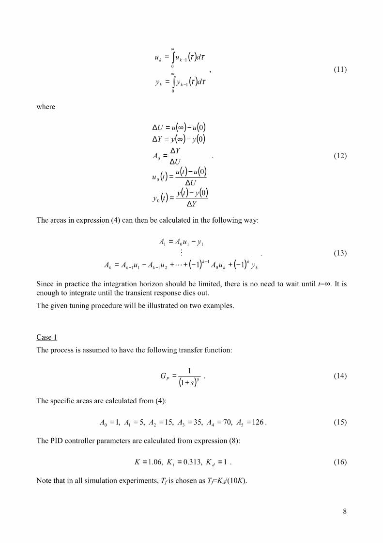
The given tuning procedure will be illustrated on two examples. Case 1
The process is assumed to have the following transfer function:
( )51
1s
GP += . (14)
The specific areas are calculated from (4):
126 ,70 ,35 ,15 ,5 ,1 543210 ====== AAAAAA . (15)
The PID controller parameters are calculated from expression (8):
1 ,313.0 ,06.1 === di KKK . (16)
Note that in all simulation experiments, Tf is chosen as Tf=Kd/(10K).
9
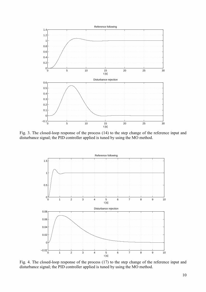
Fig. 3. shows the closed-loop response on reference change and input-disturbance. Note that the closed-loop response features relatively good tracking performance and disturbance rejection.
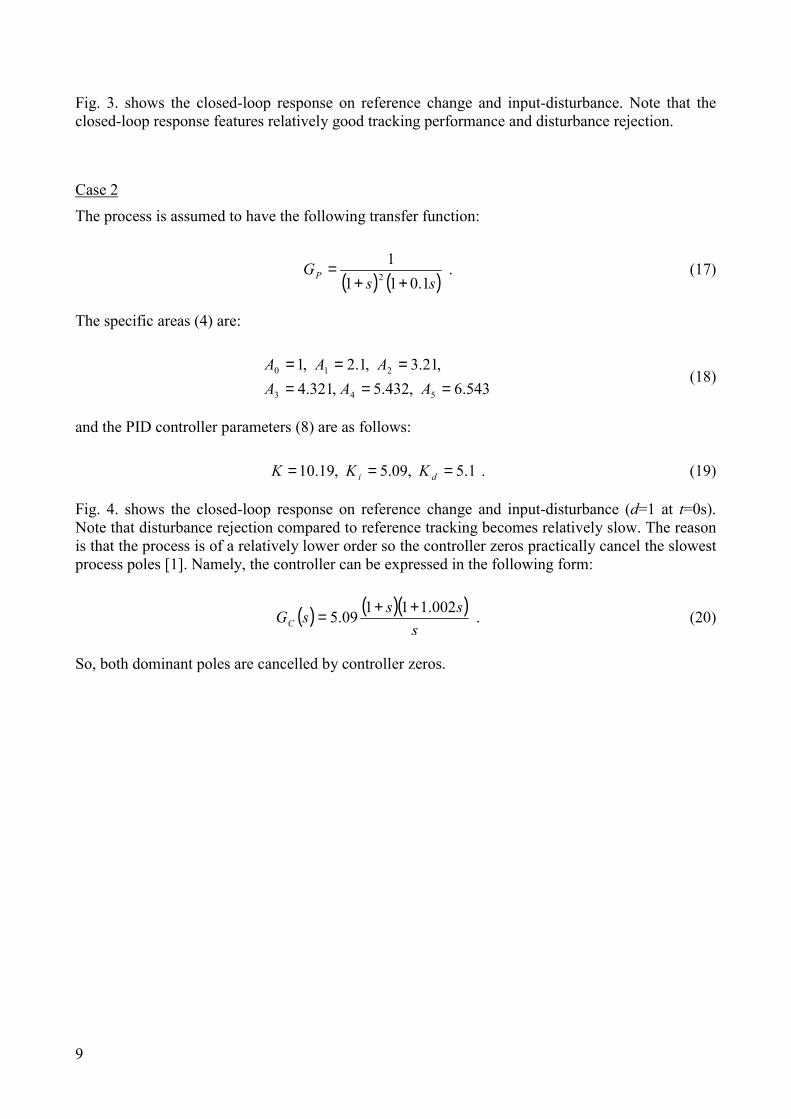
Case 2
The process is assumed to have the following transfer function:
( ) ( )ss
GP 1.0111
2 ++= . (17)
The specific areas (4) are:
543.6 ,432.5 ,321.4
,21.3 ,1.2 ,1
543
210
======
AAAAAA
(18)
and the PID controller parameters (8) are as follows:
1.5 ,09.5 ,19.10 === di KKK . (19)
Fig. 4. shows the closed-loop response on reference change and input-disturbance (d=1 at t=0s). Note that disturbance rejection compared to reference tracking becomes relatively slow. The reason is that the process is of a relatively lower order so the controller zeros practically cancel the slowest process poles [1]. Namely, the controller can be expressed in the following form:
( ) ( )( )s
sssGC002.11109.5 ++= . (20)
So, both dominant poles are cancelled by controller zeros.
10
0 5 10 15 20 25 300
0.2
0.4
0.6
0.8
1
1.2
1.4Reference following
t [s]
0 5 10 15 20 25 30−0.1
0
0.1
0.2
0.3
0.4
0.5
0.6Disturbance rejection
t [s] Fig. 3. The closed-loop response of the process (14) to the step change of the reference input and disturbance signal; the PID controller applied is tuned by using the MO method.
0 1 2 3 4 5 6 7 8 9 100
0.5
1
1.5
Reference following
t [s]
0 1 2 3 4 5 6 7 8 9 10−0.02
0
0.02
0.04
0.06
0.08Disturbance rejection
t [s] Fig. 4. The closed-loop response of the process (17) to the step change of the reference input and disturbance signal; the PID controller applied is tuned by using the MO method.
11
3. The disturbance-rejection MO (DRMO) method for PID controller
In the previous section it was shown that, by using the original MO method, disturbance rejection is degraded when dealing with lower-order processes, since slow process poles are almost entirely cancelled by controller zeros.
This is not unusual, since the MO method aims at achieving good reference tracking, so it optimises the transfer function GCL(s)=Y(s)/W(s) instead of GCLD(s)=Y(s)/D(s). Let us now express GCL(s) in terms of GCLD(s):
( ) ( ) ( )
( )
( )
++=
=
++=
==
2
2
1
1
sKK
sKKsG
sKK
sKK
sK
sG
sGsGsG
i
d
iCLO
i
d
i
iCLD
CCLDCL
, (21)
where
( ) ( )( ) ( ) s
KsGsG
sGsG i
CP
PCLO +
=1
. (22)
From expression (21) it can be seen that controller’s zeros (the sub-expression in brackets) play an important role within GCL(s), which is actually “optimised” by the original MO method. On the other hand, controller’s zeros may significantly degrade disturbance rejection performance. A strategy proposed herein is to optimise the transfer function GCLO(s) (22) instead of GCL(s) in expression (1).
The number of conditions which can be satisfied in expression (1) depends on controller order [20]. Namely, by using the PID controller (three independent controller parameters), the first three derivatives (r=1,2,3) can be satisfied. Note that the first expression (GCL(0)=1) is already satisfied since the controller contains an integral term (under condition that the closed-loop response is stable).
By placing GCLO(s) in expression (1), the following set of equations are obtained (for r=1,2 and 3):
01222 12
0022
0 =+−−+ idi KAKKAKAKA (23)
0222224 212
20321
22120
220 = KKAAKAKAKAKAKAKAKAKA diididd −−+−+++ (24)
042
2222422
3122
12
2
22054340
231
222
240
= KKAAKAKKA
KAAKKAAKAKKAAKAAKAKAA
idddi
diddi
++−
−−−+−−−+ (25)
Since in each equation, the parameters K and Ki are of the second order, the final result can be obtained usually by means of optimisation (it cannot be solved analytically). The proper solution should fulfil the following conditions:
• K should be a real number (K∈ℜ ) and should not exceed some pre-defined range of values.
12
• The chosen Ki together with K and Kd should have the same sign as the process steady-state gain (KPR or A0).
Initial values for the optimisation are the values calculated by using expressions (8). Any method of optimisation (iterative search for numeric solution) that solves the system of nonlinear equations can be applied.
Possible practical tuning procedure is to calculate derivative gain from expression (8), then calculate proportional gain K from equations (23) and (24):
( ) ( )
026224
444442234
02
12
02
1320
22
0212
10302
2103
132
0
=++++
++−−+−+
dddd
dd
KAKAAKAAKAA
KKAAAAKAAAAKAAAAAA . (26)
Integral gain Ki can be then calculated from equation (23):
( )( )d
i KAAKA
K 201
20
21
++
= . (27)
Then equation (25) should be tested. Derivative gain should be modified and K (26) and Ki (27) re-calculated until equation (25) becomes zero. One of the simplest solutions for the calculation of controller parameters is to use some simple search methods like Newton’s. In most cases only few iterations are required for achieving very accurate result. MATLAB files which calculate optimal PID controller parameters for disturbance rejection (according to expressions (23) to (25)) are given in appendix and in [24].
Such tuning procedure is also called disturbance-rejection MO (DRMO) method.
Calculation of PI controller parameters is simpler, since Kd is fixed to Kd=0. Then K and Ki are calculated from expressions (26) and (27).
To sum up, the DRMO tuning procedure goes as follows:
1. Calculate characteristic areas from the process transfer function (4) or from the process steady-state change (13),
2. calculate PID controller parameters (8) by using the original MO method (only for PID controllers),
3. calculate gains of the proportional and the integral term from expressions (26) and (27). For the PI controller, replace Kd with 0.
4. Test expression (25). Appropriately modify Kd and repeat steps 3 and 4 until (25) is satisfied.
The given tuning procedure will be illustrated on two examples.
Case 3
The process is assumed to have the same transfer function as in Case 1. The obtained PID controller parameters were calculated by using described tuning procedure (the optimisation was performed in program package Matlab [24]).
The obtained controller parameters were the following:
10.1 ,43.0 ,29.1 === di KKK . (28)
13
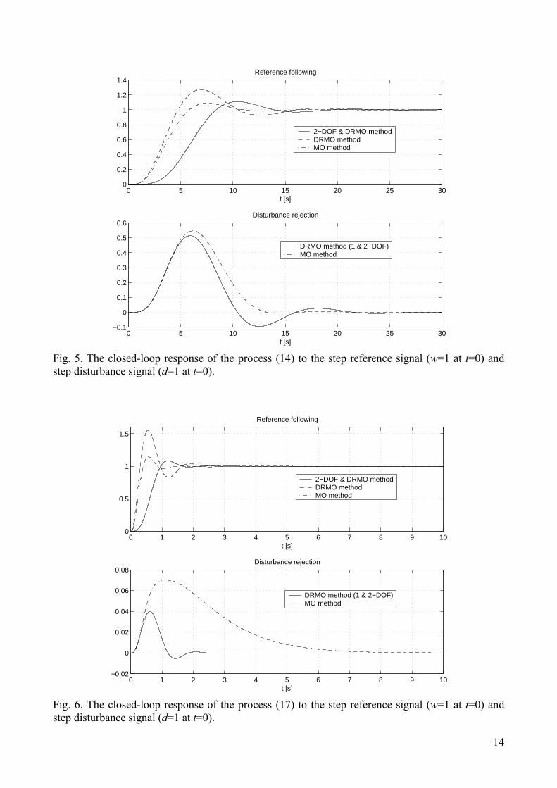
The calculated parameters are similar to those given in expression (16). It is therefore expected that tracking and disturbance rejection performance will remain almost the same to Case 1. This assumption is confirmed by the closed-loop responses given in Fig. 5 (see solid lines).
Case 4
The process is assumed to have the same transfer function as in Case 2.
The obtained controller parameters were the following:
10.5 ,57.44 ,3.24 === di KKK . (29)
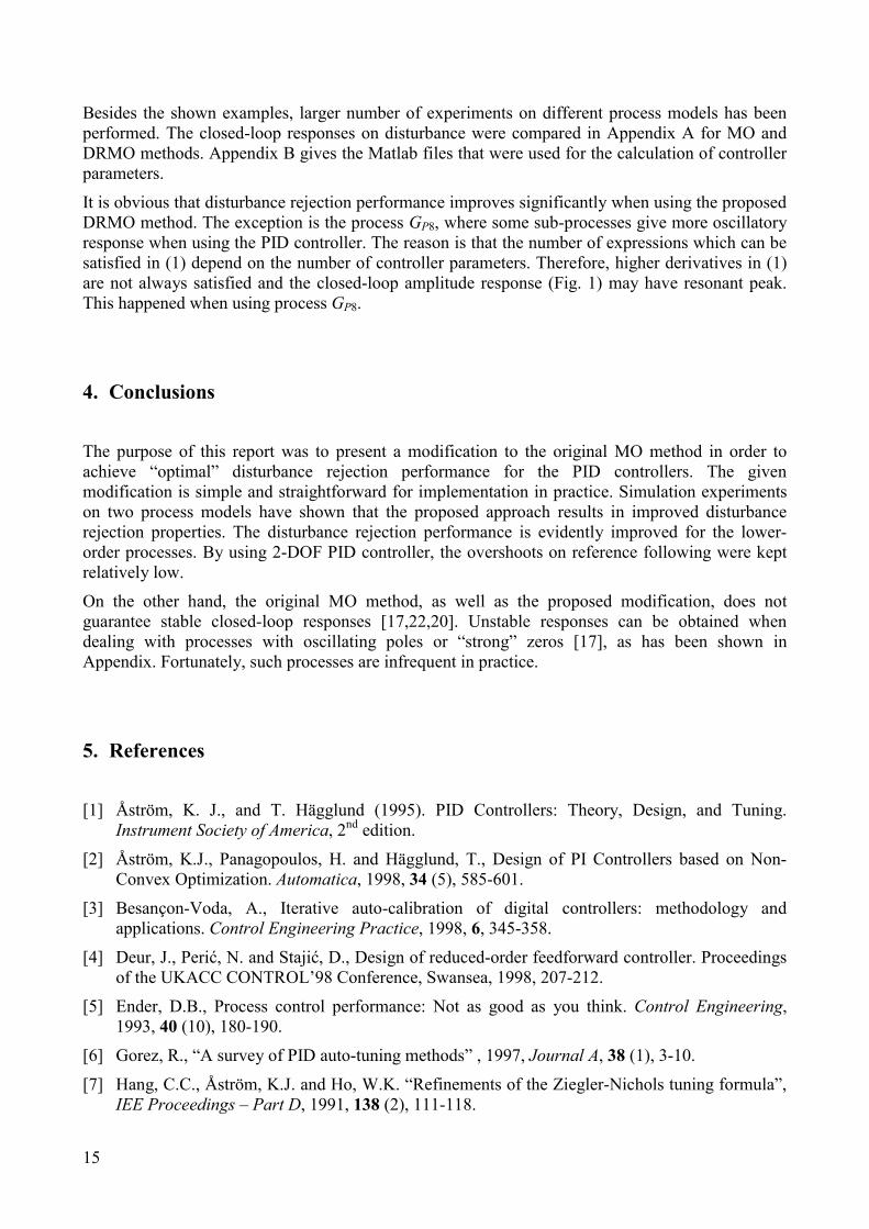
The calculated PID controller parameters are now quite different from ones given in (19). Note that the integral gain (Ki) is now much higher than before, so relatively high change of disturbance rejection performance might be expected. The closed-loop responses on reference change (w=1 at t=0) and disturbance (d=1 at t=0s) are given in Fig. 6 (solid lines). It can be seen that disturbance rejection is now quite improved in comparison to the original MO method (see Fig. 4).
However, improved disturbance rejection has its price. Namely, enlarged process overshoots after reference change can be noticed especially in Figure 6. The only way of improving deteriorated tracking performance while retaining the obtained disturbance rejection performance is using two-degrees-of-freedom (2-DOF) PID controller. One of the most simple solutions is to use the set-point weighting approach [1]. Only the integral term has been connected to the control error, while proportional and derivative terms were connected to the process output only:
( ) ( ) ( )sYsT
sKKsE
sK
sUf
di
++−=
1. (30)
Figures 5 and 6 show tracking performance when using 2-DOF PID controller (see dashed lines). The overshoots on reference following are now quite lower than when using a conventional PID controller.
14
0 5 10 15 20 25 300
0.2
0.4
0.6
0.8
1
1.2
1.4Reference following
t [s]
2−DOF & DRMO methodDRMO method MO method
0 5 10 15 20 25 30−0.1
0
0.1
0.2
0.3
0.4
0.5
0.6Disturbance rejection
t [s]
DRMO method (1 & 2−DOF)MO method
Fig. 5. The closed-loop response of the process (14) to the step reference signal (w=1 at t=0) and step disturbance signal (d=1 at t=0).
0 1 2 3 4 5 6 7 8 9 100
0.5
1
1.5
Reference following
t [s]
2−DOF & DRMO methodDRMO method MO method
0 1 2 3 4 5 6 7 8 9 10−0.02
0
0.02
0.04
0.06
0.08Disturbance rejection
t [s]
DRMO method (1 & 2−DOF)MO method
Fig. 6. The closed-loop response of the process (17) to the step reference signal (w=1 at t=0) and step disturbance signal (d=1 at t=0).
15
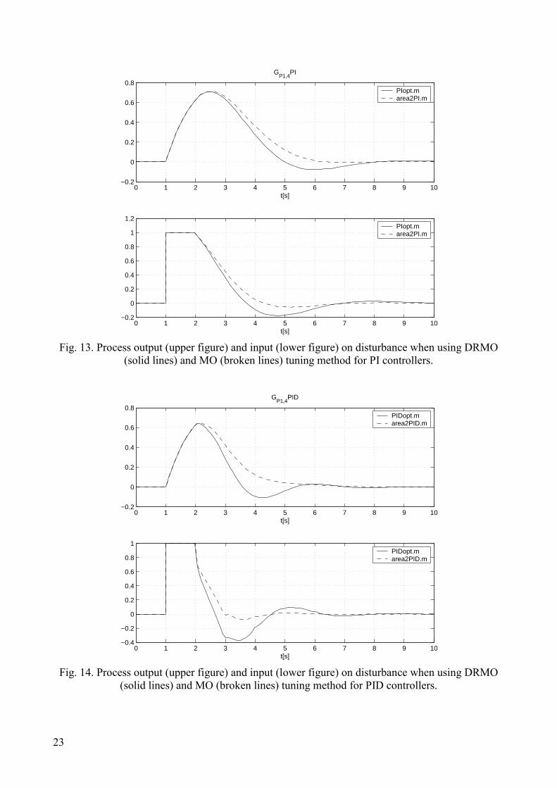
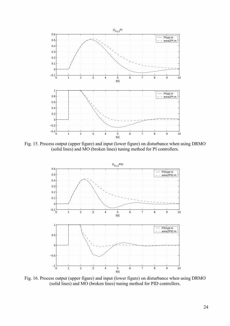
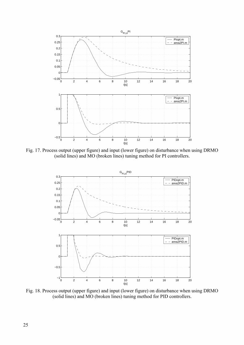
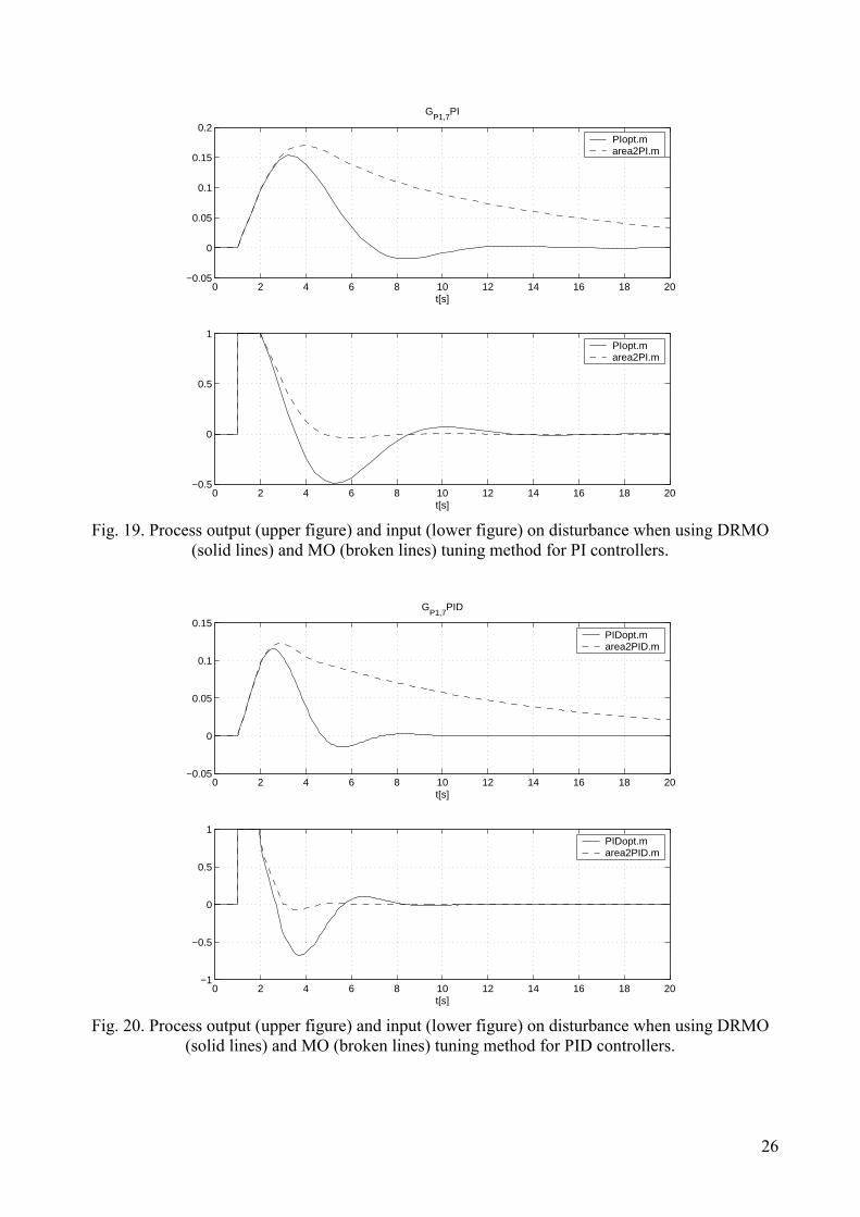
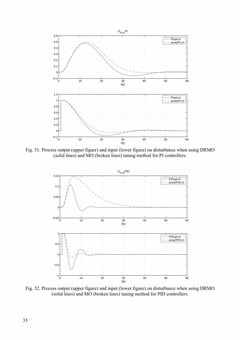
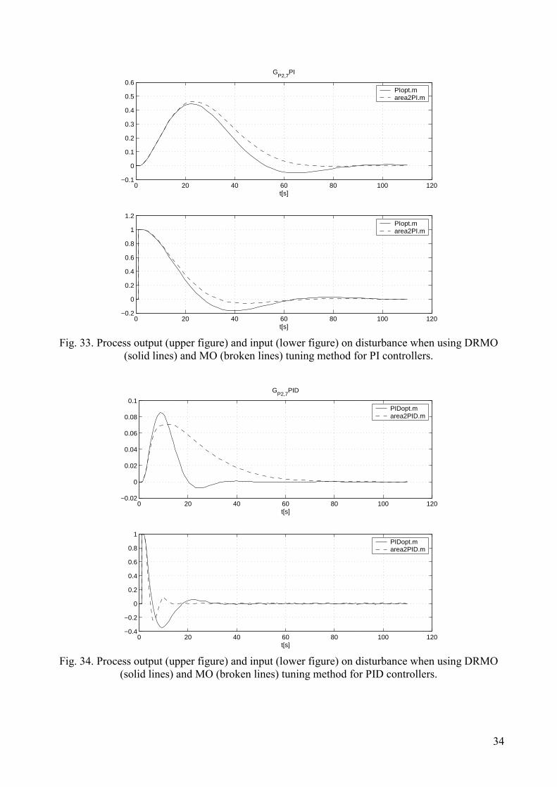
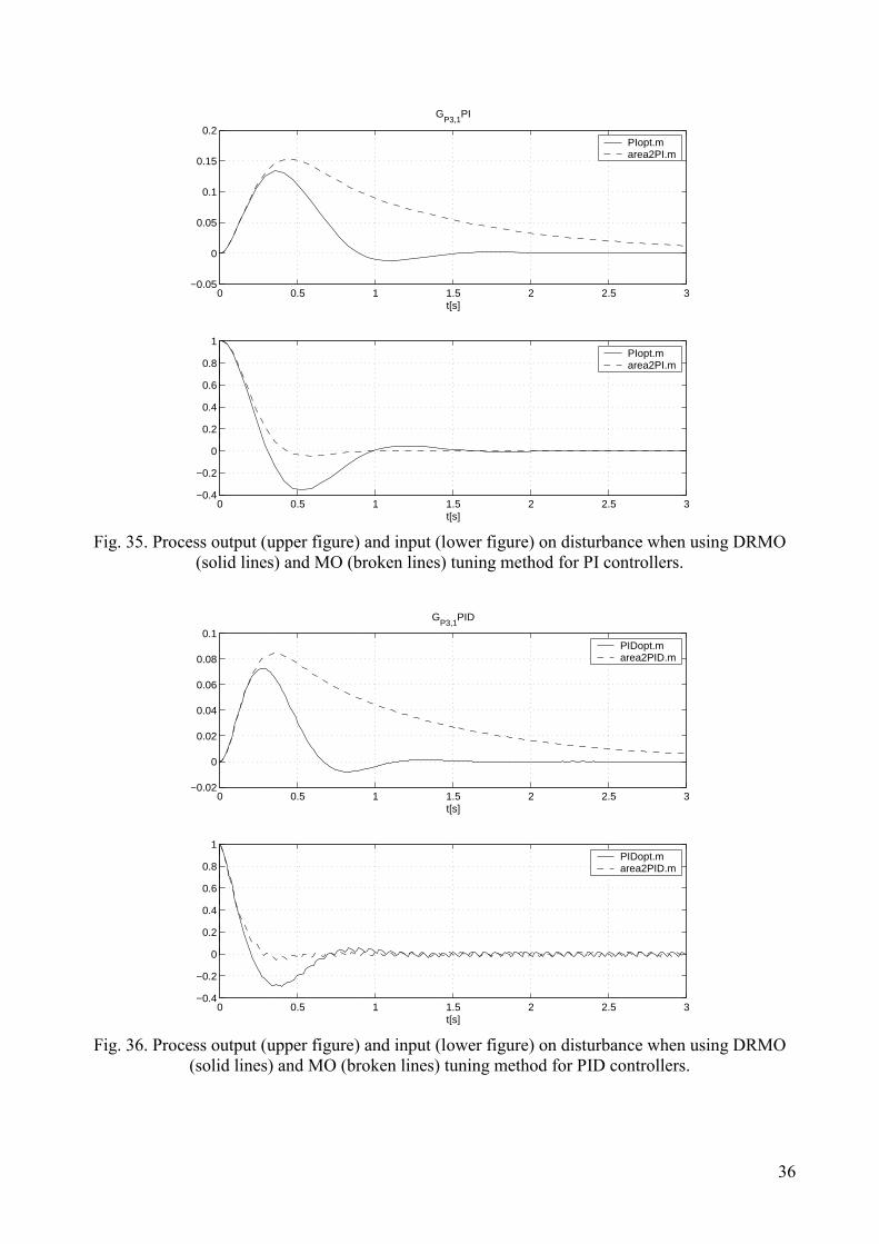
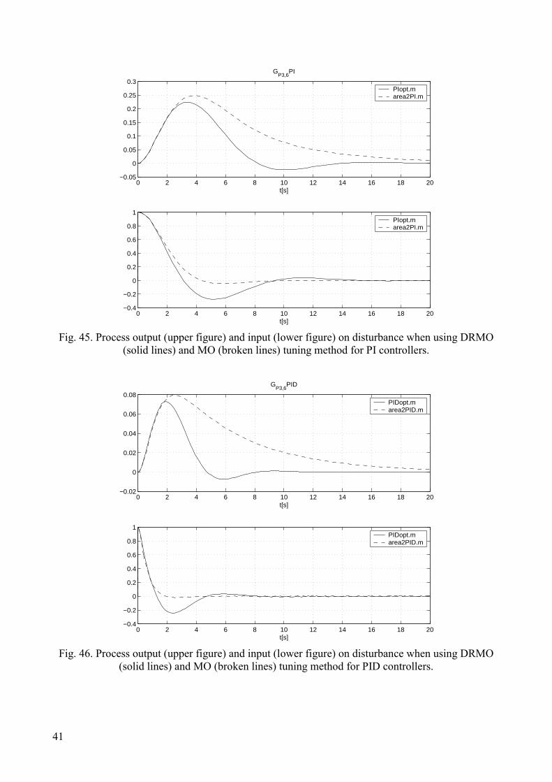
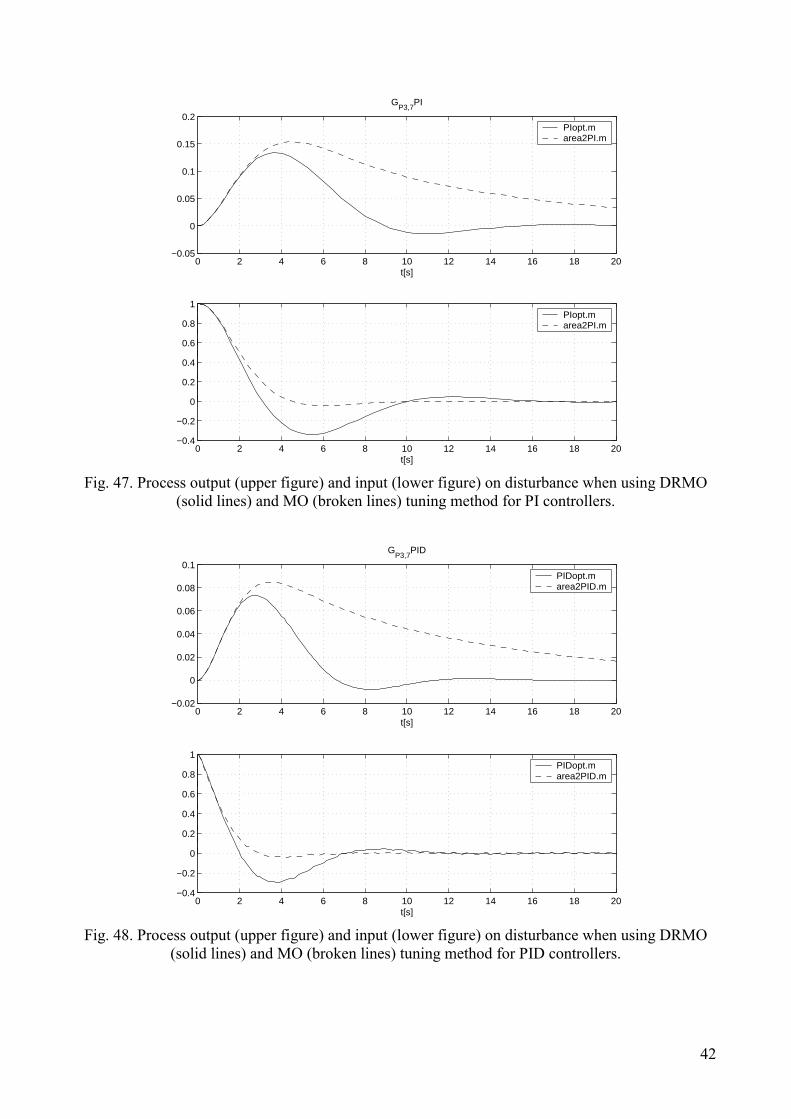
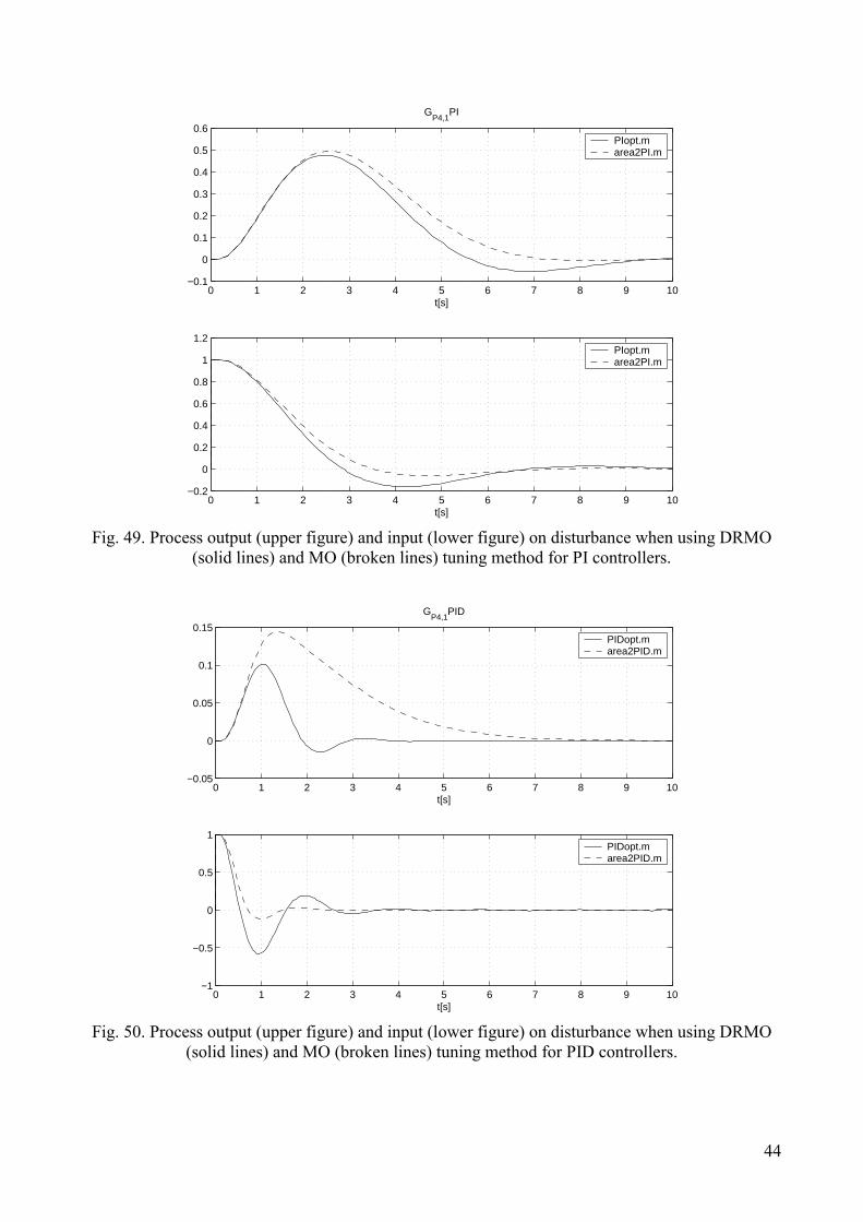
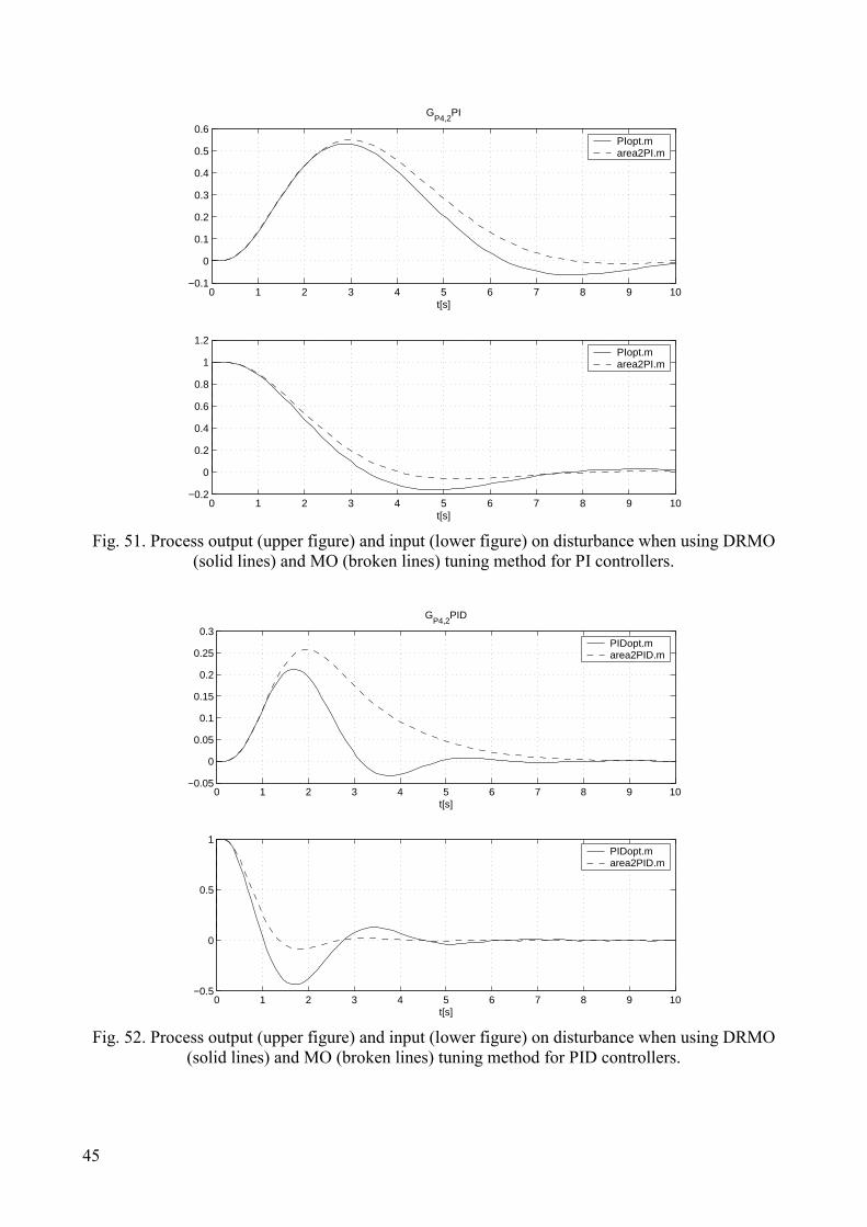
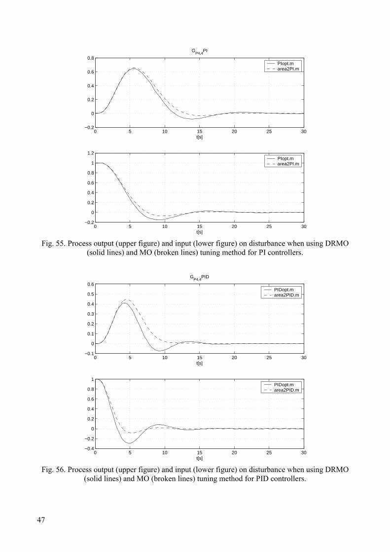
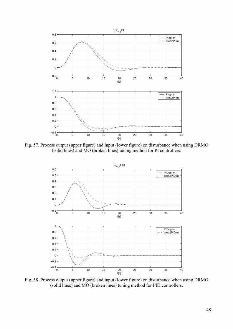
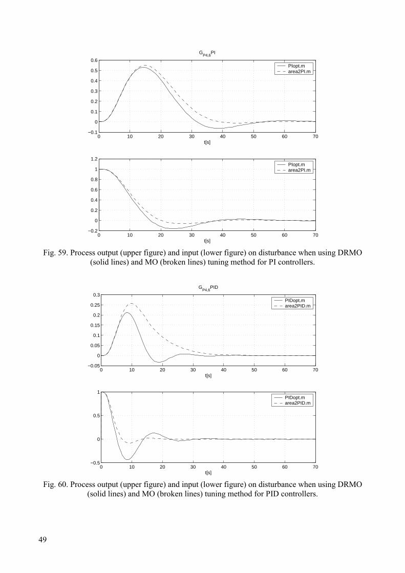
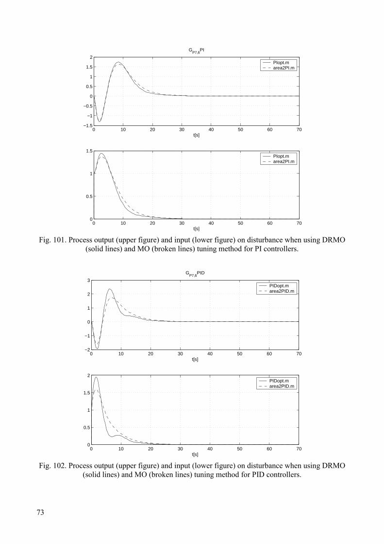
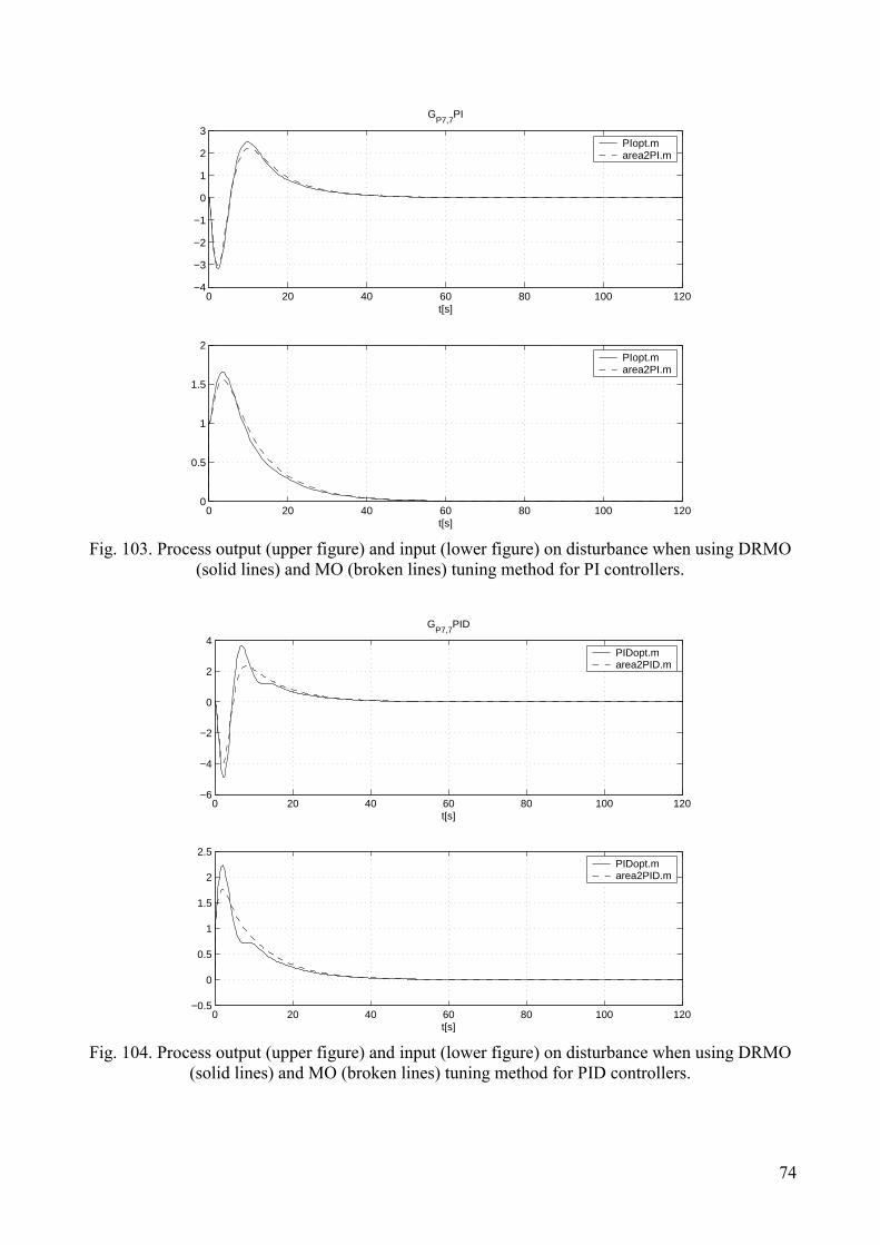
Besides the shown examples, larger number of experiments on different process models has been performed. The closed-loop responses on disturbance were compared in Appendix A for MO and DRMO methods. Appendix B gives the Matlab files that were used for the calculation of controller parameters.
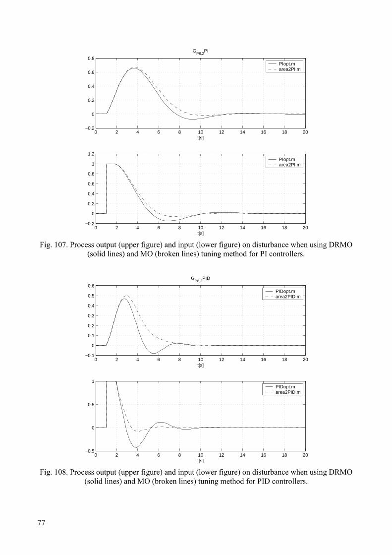
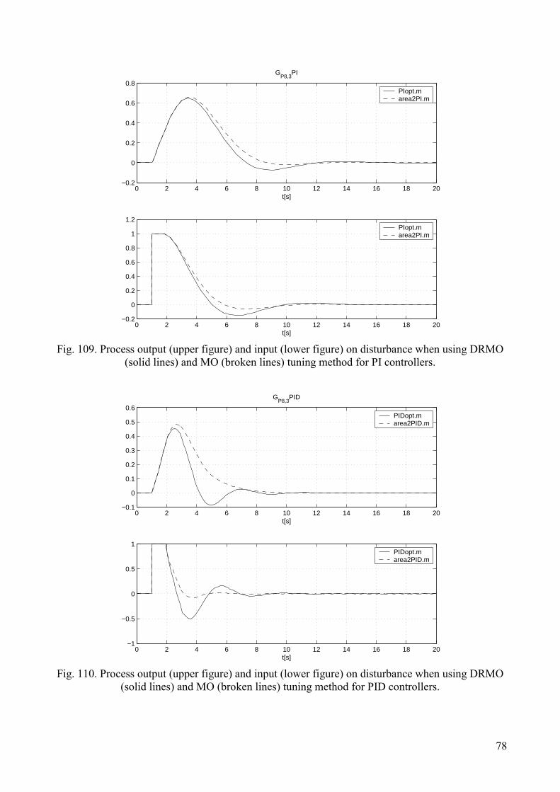
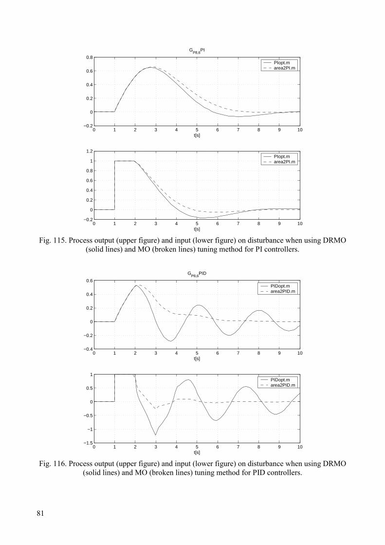
It is obvious that disturbance rejection performance improves significantly when using the proposed DRMO method. The exception is the process GP8, where some sub-processes give more oscillatory response when using the PID controller. The reason is that the number of expressions which can be satisfied in (1) depend on the number of controller parameters. Therefore, higher derivatives in (1) are not always satisfied and the closed-loop amplitude response (Fig. 1) may have resonant peak. This happened when using process GP8.
4. Conclusions
The purpose of this report was to present a modification to the original MO method in order to achieve “optimal” disturbance rejection performance for the PID controllers. The given modification is simple and straightforward for implementation in practice. Simulation experiments on two process models have shown that the proposed approach results in improved disturbance rejection properties. The disturbance rejection performance is evidently improved for the lower-order processes. By using 2-DOF PID controller, the overshoots on reference following were kept relatively low.
On the other hand, the original MO method, as well as the proposed modification, does not guarantee stable closed-loop responses [17,22,20]. Unstable responses can be obtained when dealing with processes with oscillating poles or “strong” zeros [17], as has been shown in Appendix. Fortunately, such processes are infrequent in practice.
5. References
[1] Åström, K. J., and T. Hägglund (1995). PID Controllers: Theory, Design, and Tuning. Instrument Society of America, 2nd edition.
[2] Åström, K.J., Panagopoulos, H. and Hägglund, T., Design of PI Controllers based on Non-Convex Optimization. Automatica, 1998, 34 (5), 585-601.
[3] Besançon-Voda, A., Iterative auto-calibration of digital controllers: methodology and applications. Control Engineering Practice, 1998, 6, 345-358.
[4] Deur, J., Perić, N. and Stajić, D., Design of reduced-order feedforward controller. Proceedings of the UKACC CONTROL’98 Conference, Swansea, 1998, 207-212.
[5] Ender, D.B., Process control performance: Not as good as you think. Control Engineering, 1993, 40 (10), 180-190.
[6] Gorez, R., “A survey of PID auto-tuning methods” , 1997, Journal A, 38 (1), 3-10.
[7] Hang, C.C., Åström, K.J. and Ho, W.K. “Refinements of the Ziegler-Nichols tuning formula”, IEE Proceedings – Part D, 1991, 138 (2), 111-118.
16
[8] Hanus, R. “Determination of controllers parameters in the frequency domain”, Journal A, 1975, XVI (3).
[9] Ho, W.K., Hang, C.C. and Cao, L.S. “Tuning of PID Controllers Based on Gain and Phase Margin Specifications”, 12th World Congress IFAC, Sydney, Proceedings, 1993, Vol. 5, 267-270.
[10] Kessler, C., “Über die Vorausberechnung optimal abgestimmter Regelkreise Teil III. Die optimale Einstellung des Reglers nach dem Betragsoptimum”, Regelungstechnik, 1955, 3, 40-49.
[11] Preuss, H.P., “Prozessmodellfreier PID-regler- Entwurf nach dem Betragsoptimum”, Automatisierungstechnik, 1991, 39 (1), 15-22.
[12] Shinskey, F.G. (2000). PID-deadtime control of distributed processes. Pre-prints of the IFAC Workshop on Digital Control, Terassa, pp. 14-18.
[13] Skogestad, S. “Simple analytic rules for model reduction and PID controller tuning”, Journal of process control, 2003, 13, 291-309.
[14] Strejc, V., “Auswertung der dynamischen Eigenschaften von Regelstrecken bei gemessenen Ein- und Ausgangssignalen allgemeiner Art”, Z. Messen, Steuern, Regeln, 1960, 3 (1), 7-11.
[15] Umland, J.W. and Safiuddin, M. “Magnitude and symmetric optimum criterion for the design of linear control systems: what is it and how does it compare with the others?”, IEEE Transactions on Industry Applications, 1990, 26 (3), 489-497.
[16] Voda, A. A. & I. D. Landau (1995). A Method for the Auto-calibration of PID Controllers. Automatica, 31 (1), pp. 41-53.
[17] Vrančić, D. (1997). Design of Anti-Windup and Bumpless Transfer Protection. PhD Thesis, University of Ljubljana, Ljubljana. Available on www-e2.ijs.si/Damir.Vrancic/bibliography.html
[18] Vrančić, D., and S. Strmčnik (1999). Achieving Optimal Disturbance Rejection by Using the Magnitude Optimum Method. Pre-prints of the CSCC’99 Conference, Athens, pp. 3401-3406.
[19] Vrančić, D., Peng Y. and Danz, C. “A comparison between different PI controller tuning methods”, Report DP-7286, J. Stefan Institute, Ljubljana, 1995.
Available on http://www-e2.ijs.si/Damir.Vrancic/bibliography.html
[20] Vrančić, D., S. Strmčnik, and Đ. Juričić (2001). A magnitude optimum multiple integration method for filtered PID controller. Automatica, 37, pp. 1473-1479.
[21] Vrančić, D. and Strmčnik S. “Achieving optimal disturbance rejection by means of the magnitude optimum method”, Proceedings of the CSCC'99, July 4-8, Athens, 1999, 3401-3406.
[22] Vrančić, D., Peng, Y. and Strmčnik, S. “A new PID controller tuning method based on multiple integrations”, Control Engineering Practice, 1999, 7, 623-633.
[23] Vrančić, D., Strmčnik, S. and Juričić, Đ. “A magnitude optimum multiple integration method for filtered PID controller”, Automatica, 2001, 37, 1473-1479.
[24] Vrančić, D. “Matlab functions for the calculation of controller parameters from the characteristic areas” and “Matlab Toolset for Disturbance Rejection Controller (PID)”, Available on http://www-e2.ijs.si/damir.vrancic/tools.html.
[25] Vrečko, D., Vrančić D., Juričić Đ. and Strmčnik S. “A new modified Smith predictor: the concept, design and tuning”, ISA Transactions, 2001, 40 (2), 111-121.
17
[26] Wang, Q. G., Hang C. C. and Bi Q. “Process frequency response estimation from relay feedback”, Control Engineering Practice, 1997, 5 (9), 1293-1302.
[27] Whiteley, A.L., “Theory of servo systems, with particular reference to stabilization”, The Journal of IEE, part II, 1946, 93 (34), 353-372.
18
Appendix A. Comparison of disturbance-rejection properties of original MO
and DRMO method for 63 process models
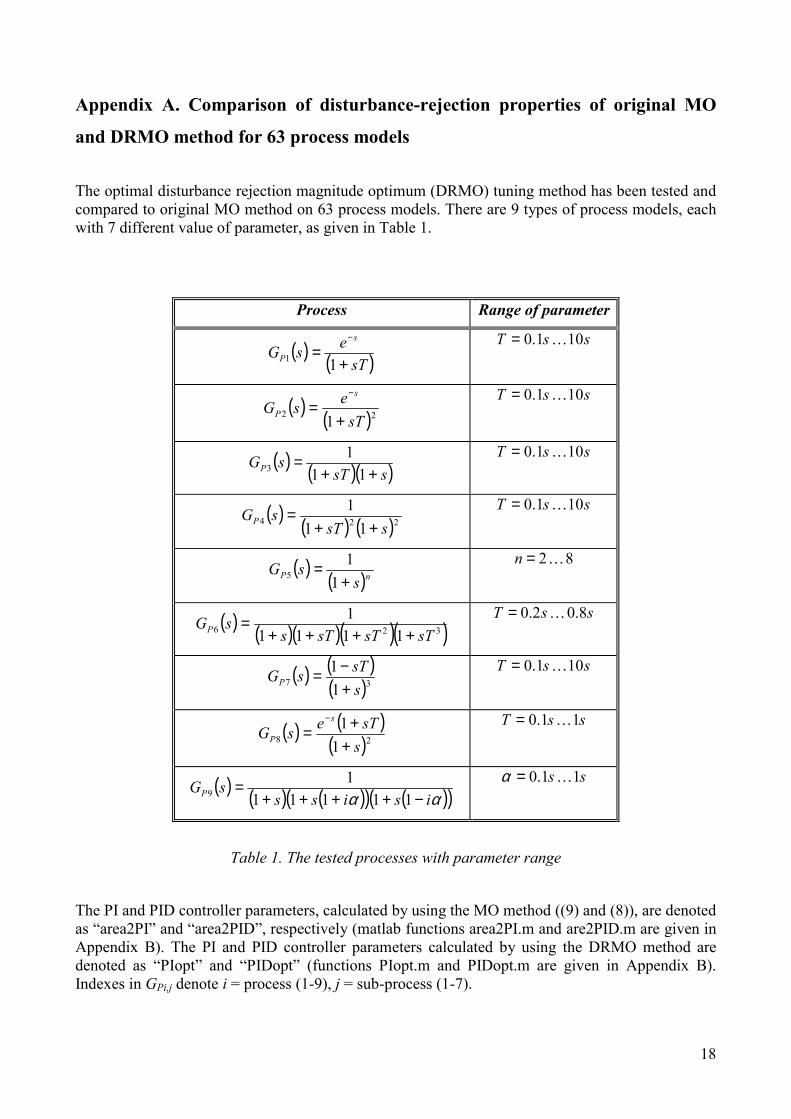
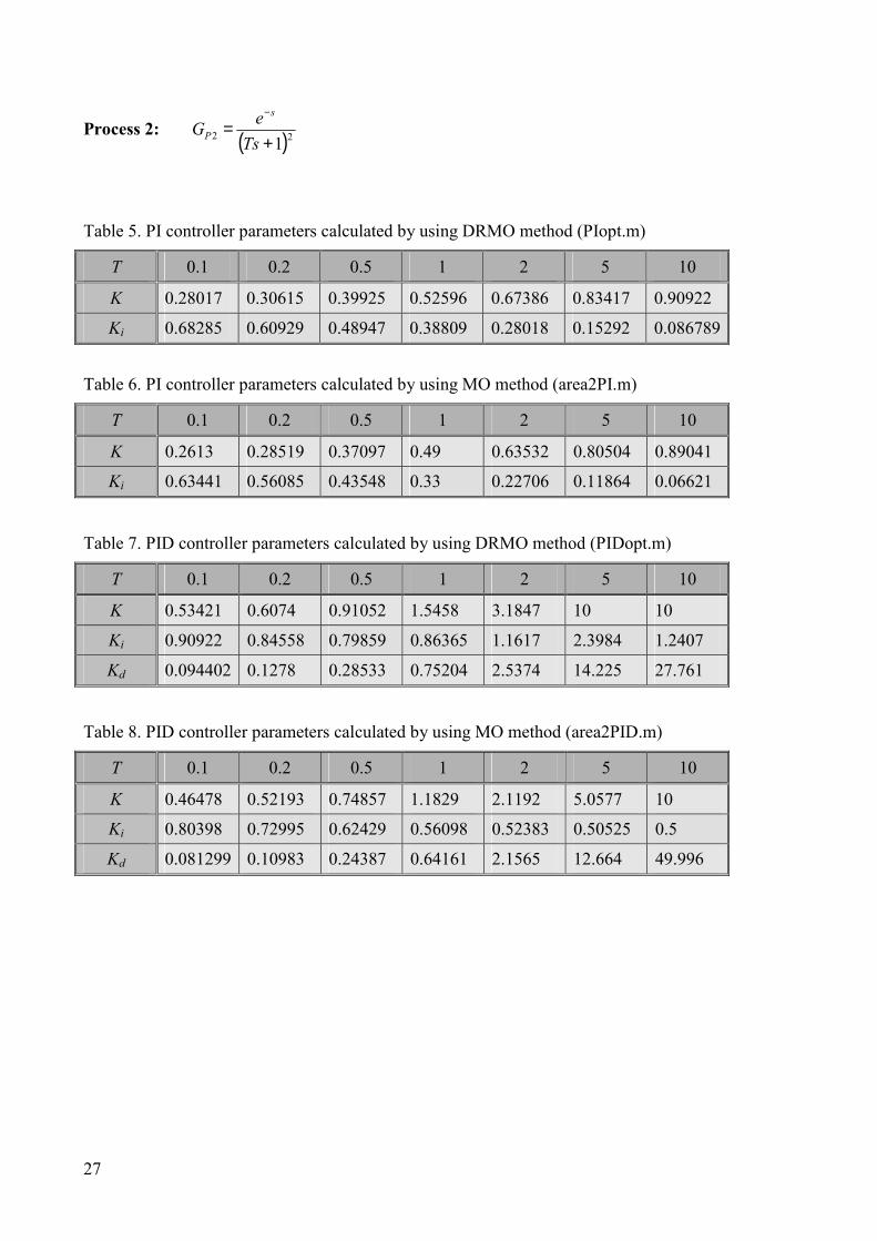
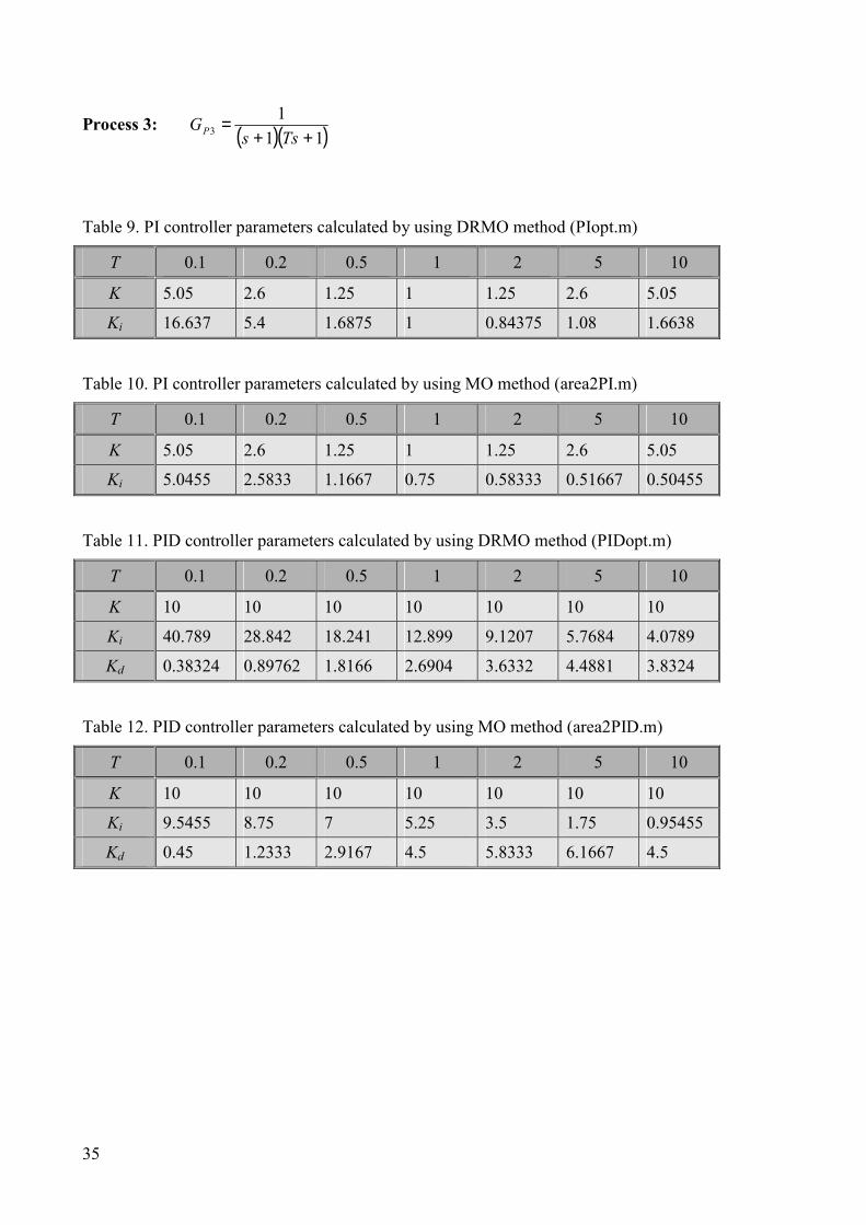
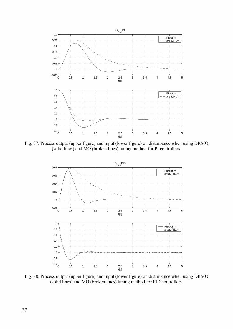
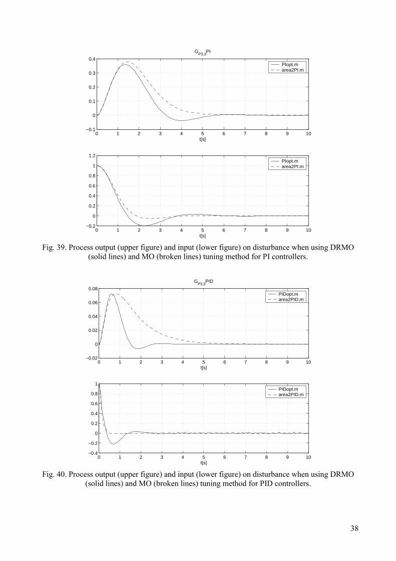
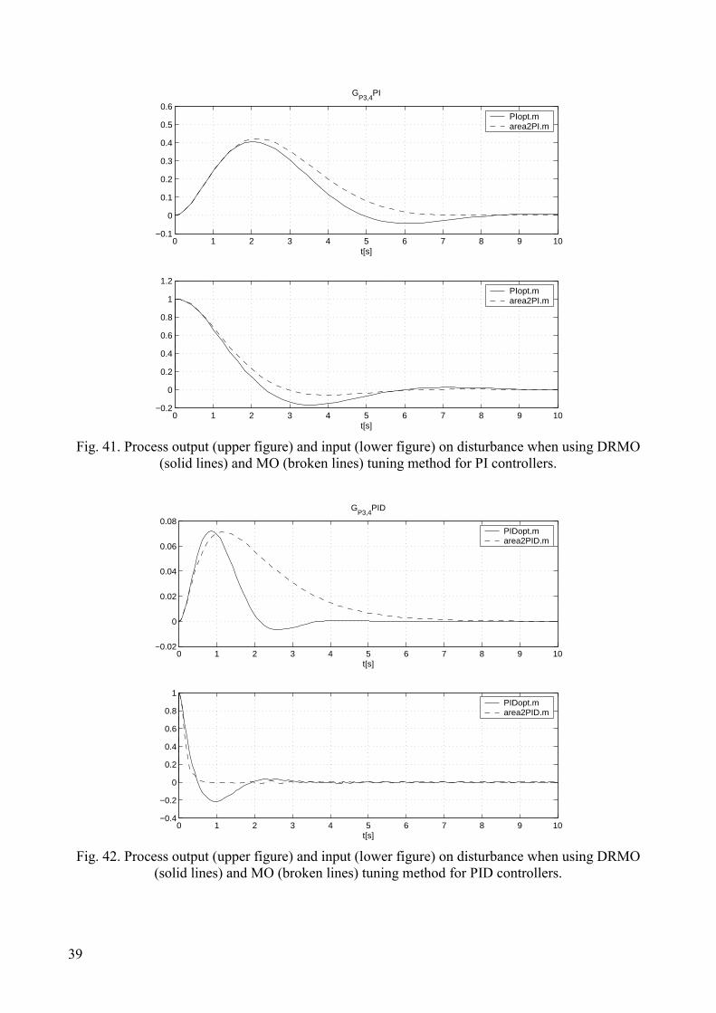
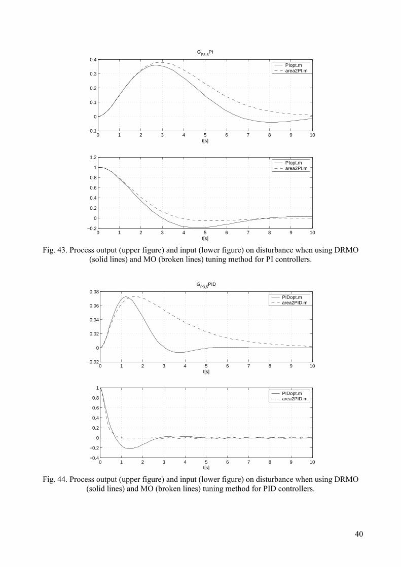
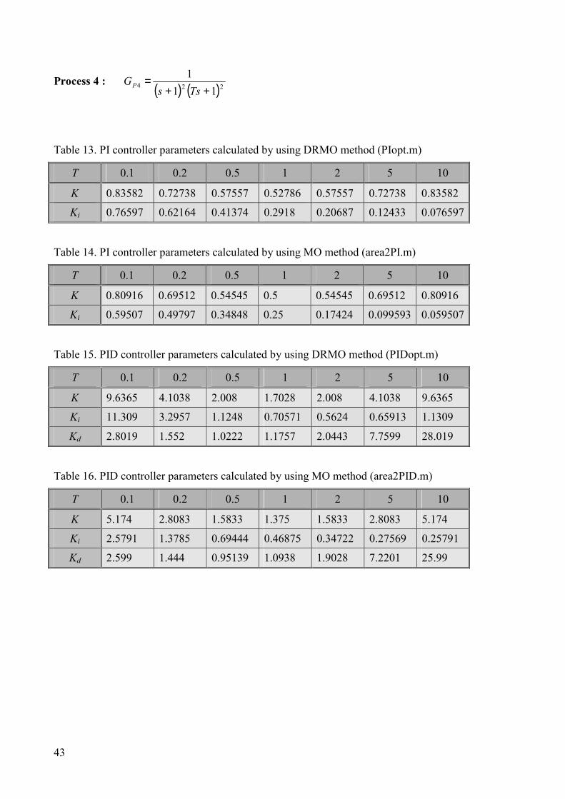
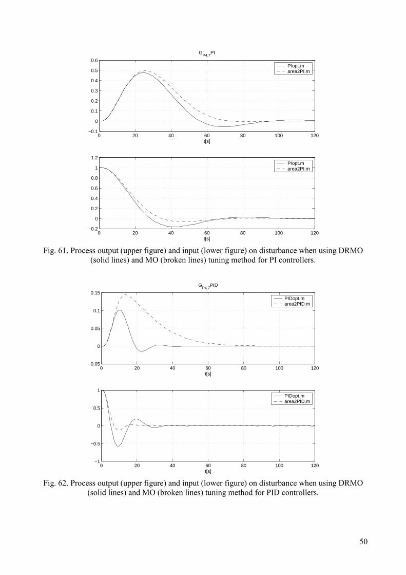
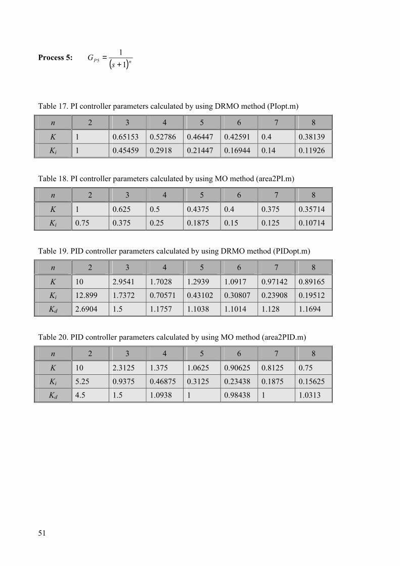
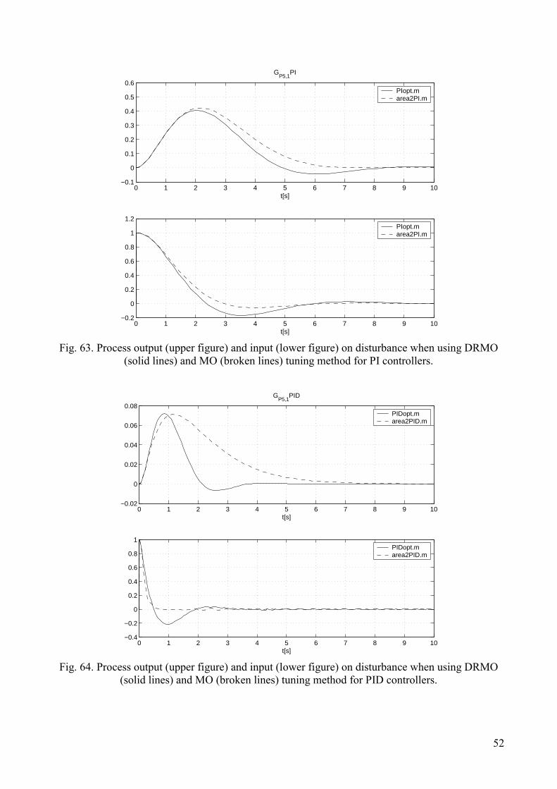
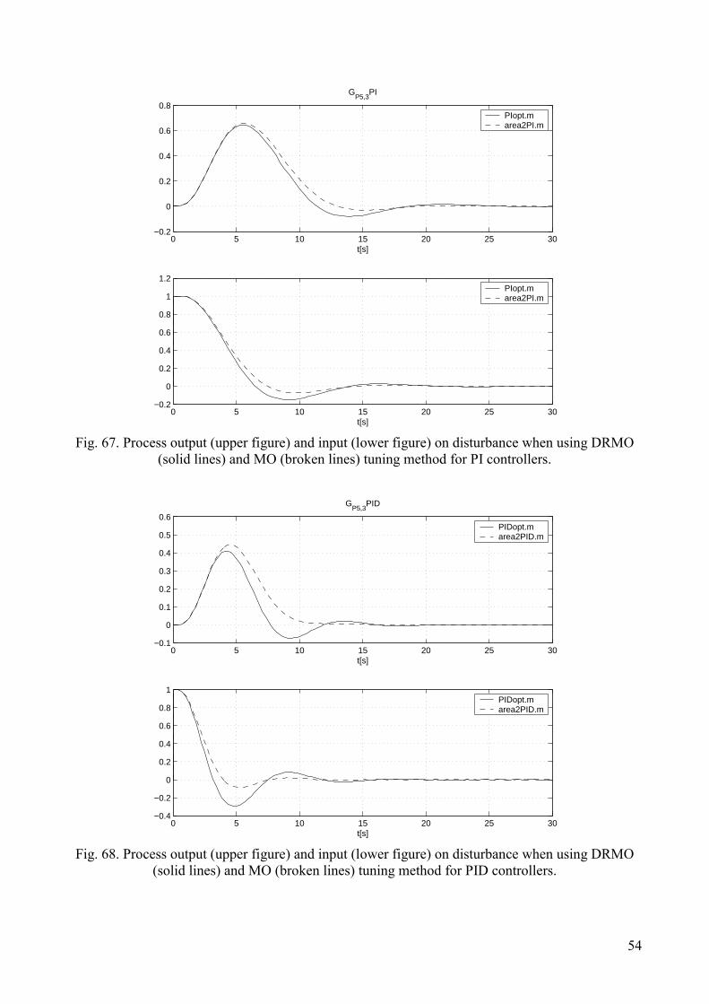
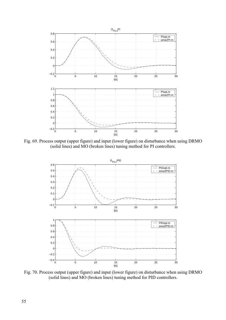
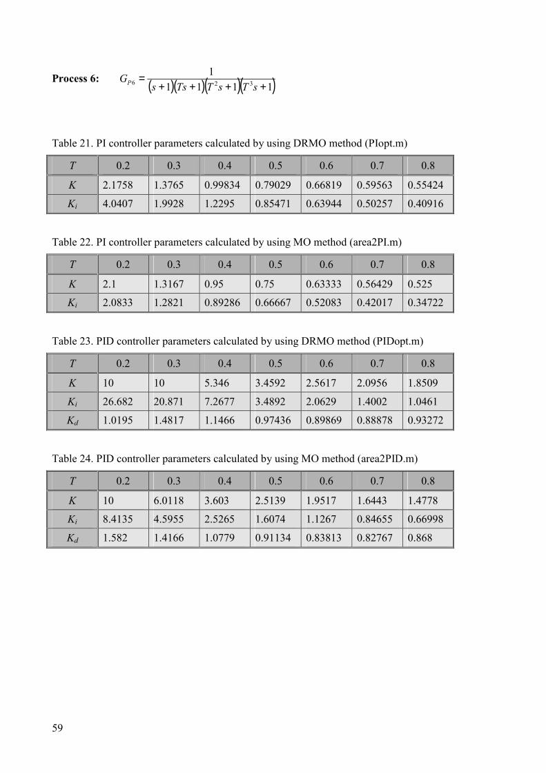
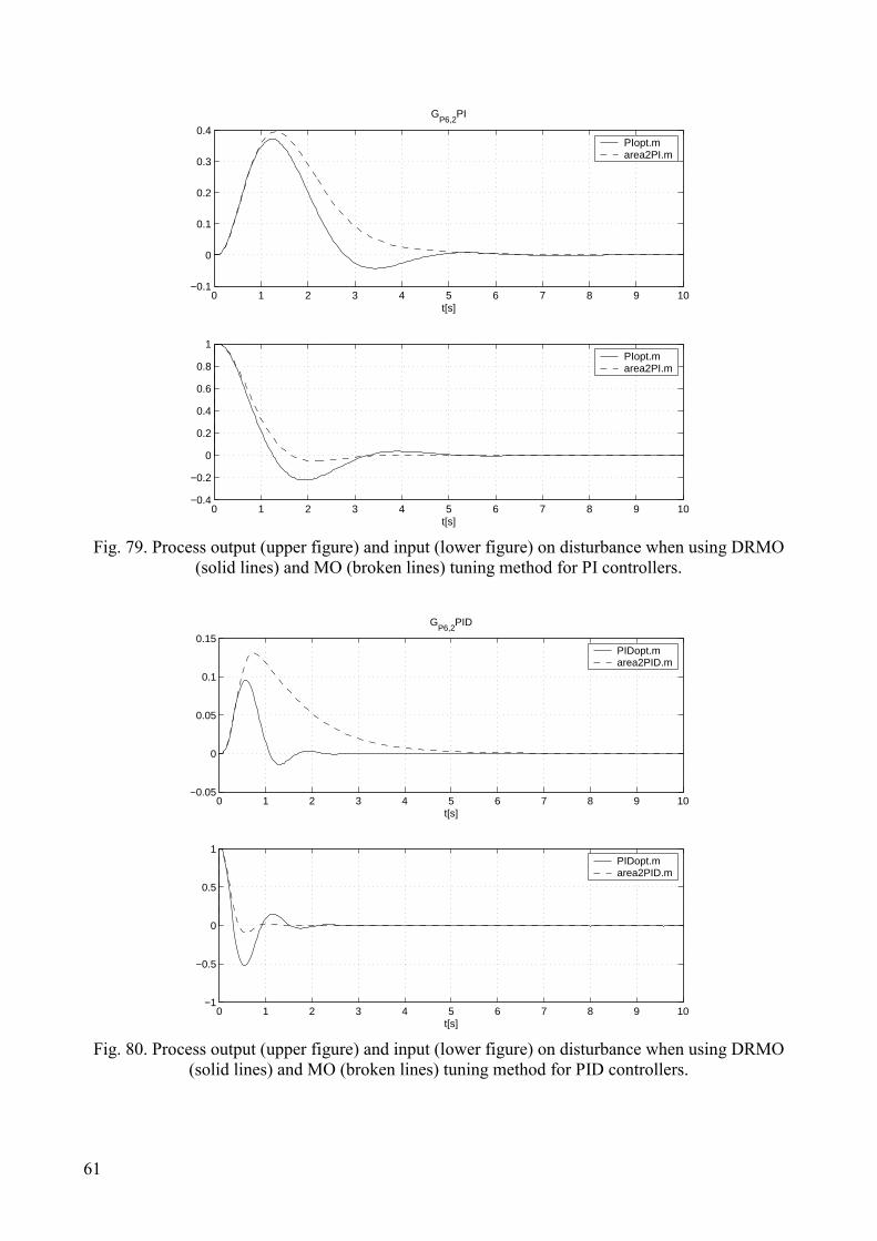
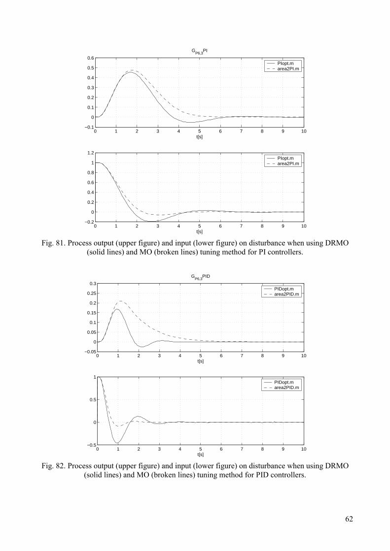
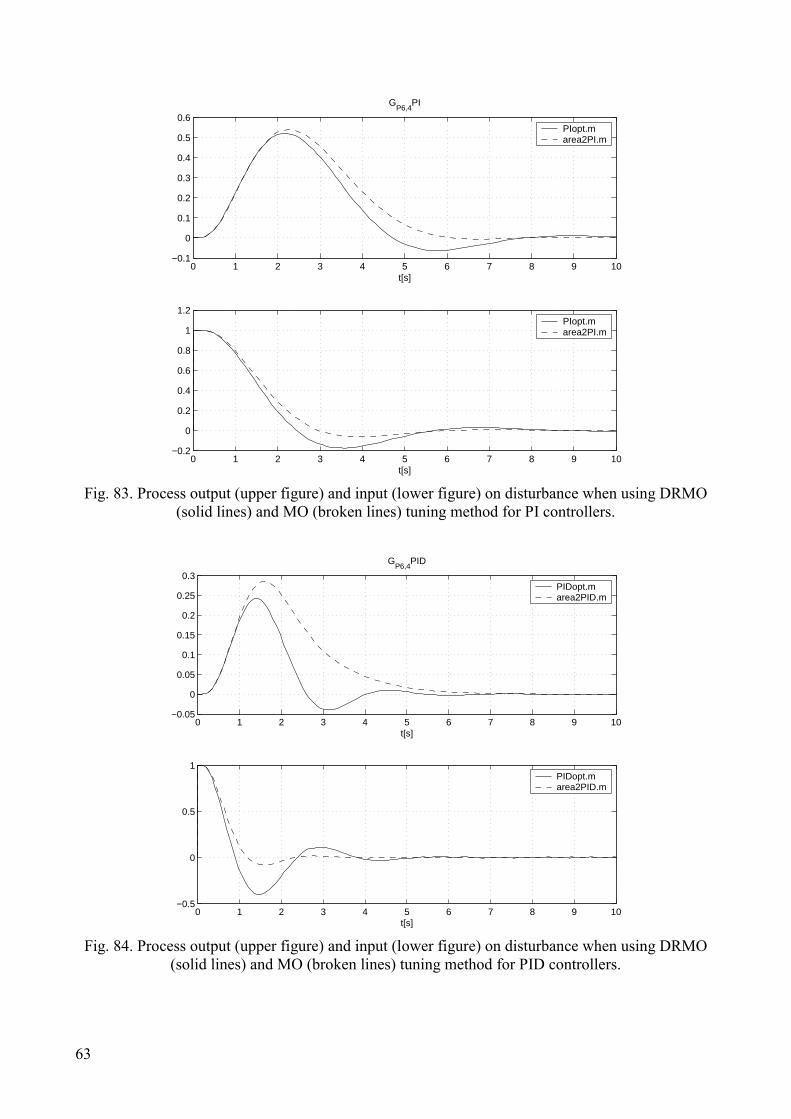
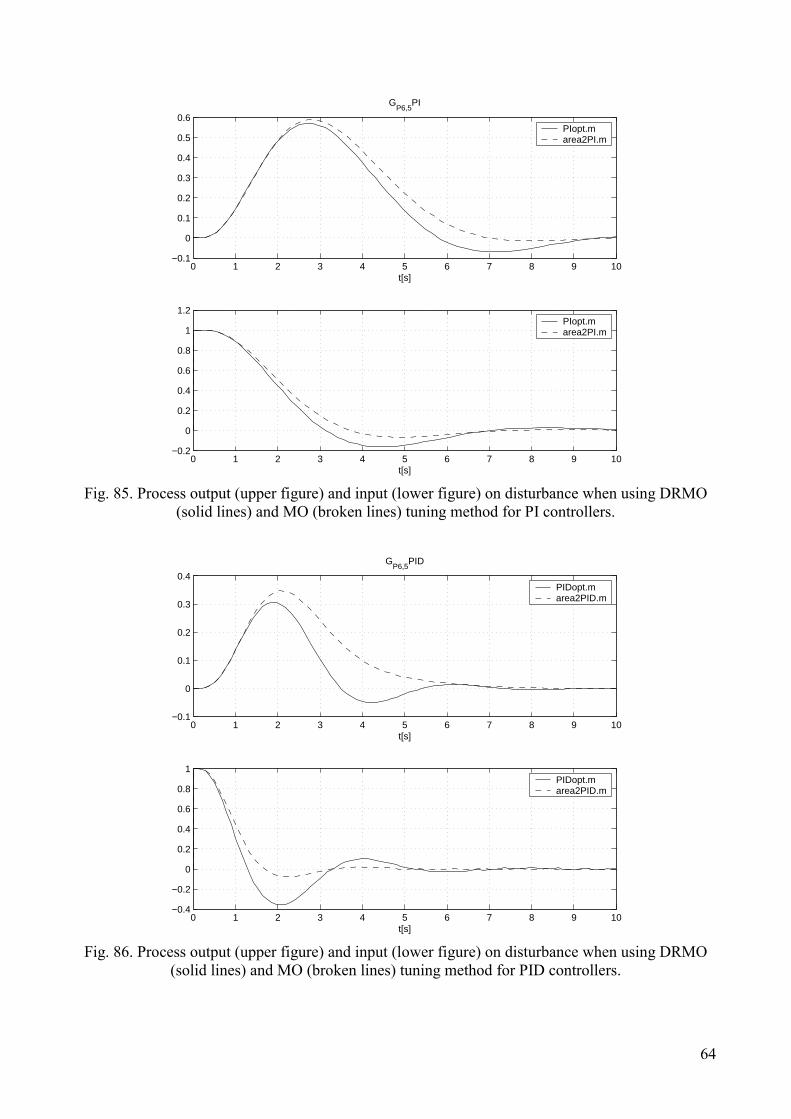
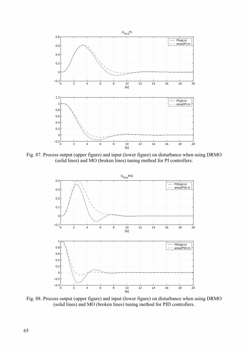
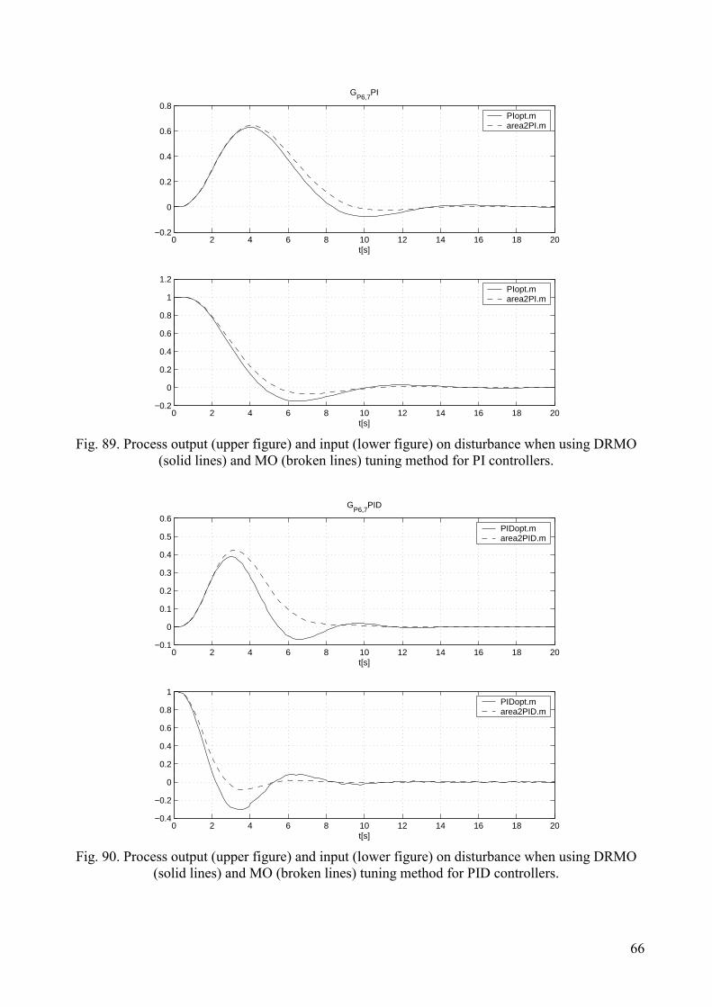
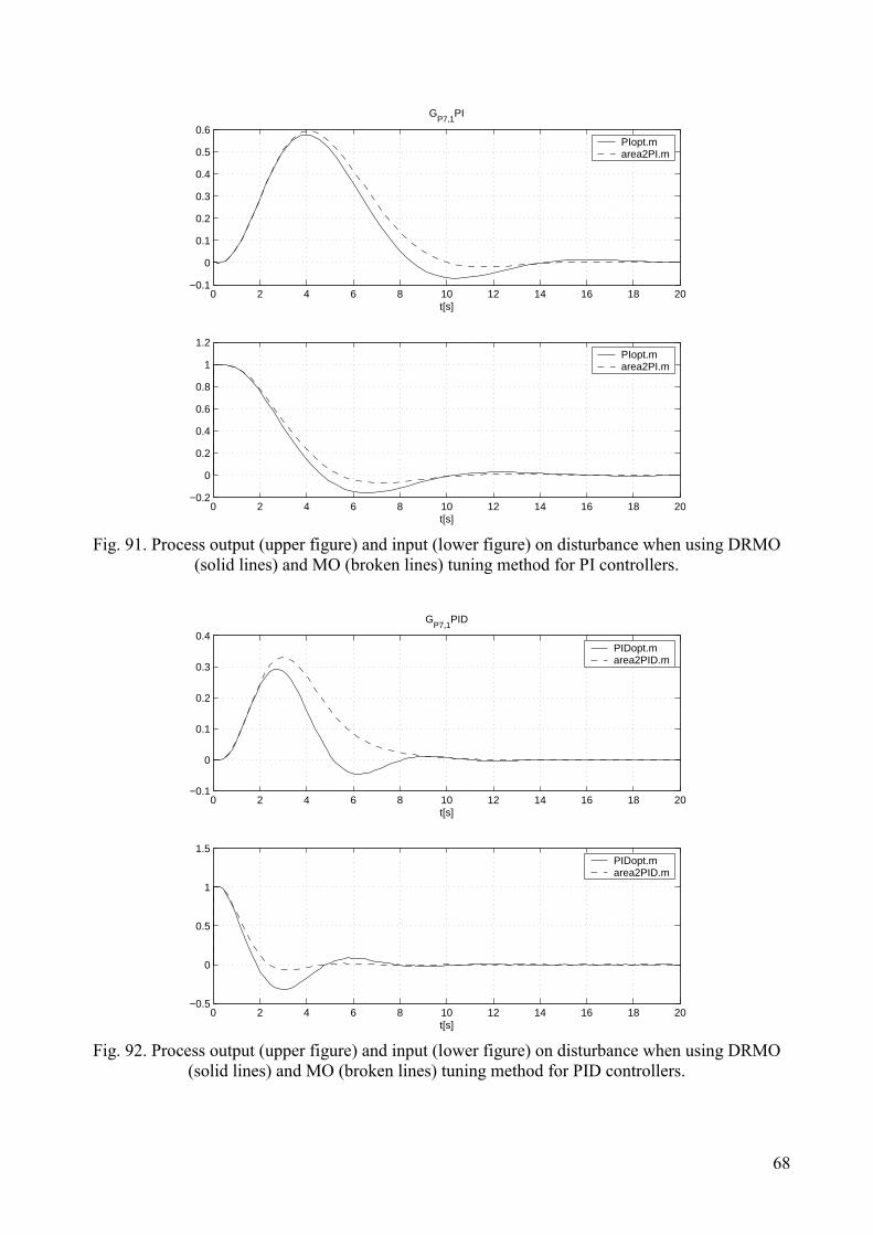
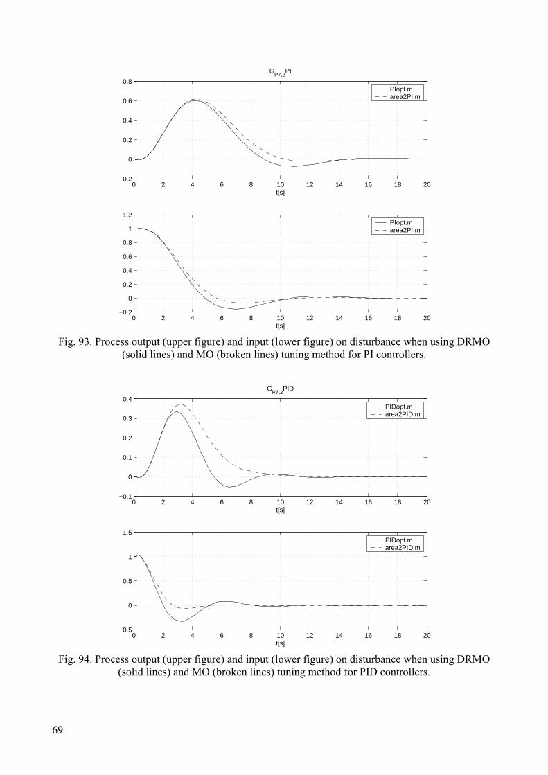
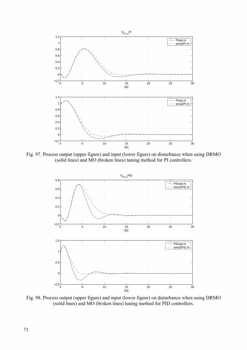
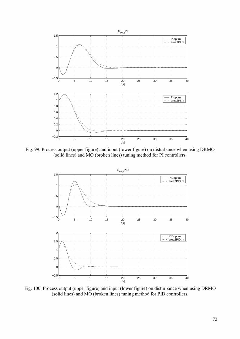
The optimal disturbance rejection magnitude optimum (DRMO) tuning method has been tested and compared to original MO method on 63 process models. There are 9 types of process models, each with 7 different value of parameter, as given in Table 1.
Process Range of parameter
( ) ( )sTesG
s
P +=
−
11 ssT 10 1.0 K=
( ) ( )22 1 sTesG
s
P +=
−
ssT 10 1.0 K=
( ) ( )( )ssTsGP ++
=11
13
ssT 10 1.0 K=
( ) ( ) ( )224 111
ssTsGP ++
= ssT 10 1.0 K=
( ) ( )nP ssG
+=
11
5 8 2K=n
( ) ( )( )( )( )326 11111
sTsTsTssGP ++++
= ssT .80 2.0 K=
( ) ( )( )37 11
ssTsGP +
−= ssT 10 1.0 K=
( ) ( )( )28 1
1s
sTesGs
P ++=
−
ssT 1 1.0 K=
( ) ( ) ( )( ) ( )( )αα isisssGP −++++
=11111
19
ss 1 1.0 K=α
Table 1. The tested processes with parameter range
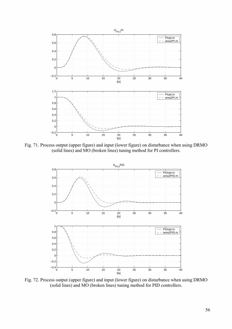
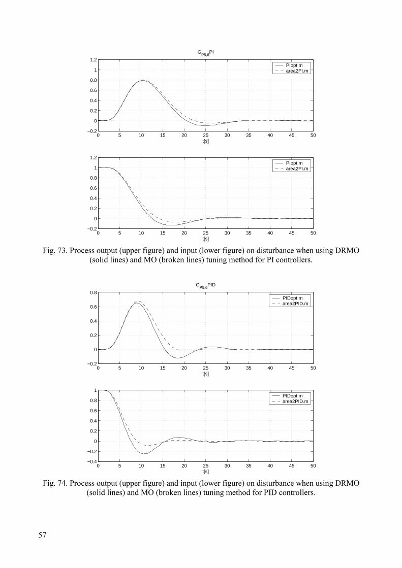
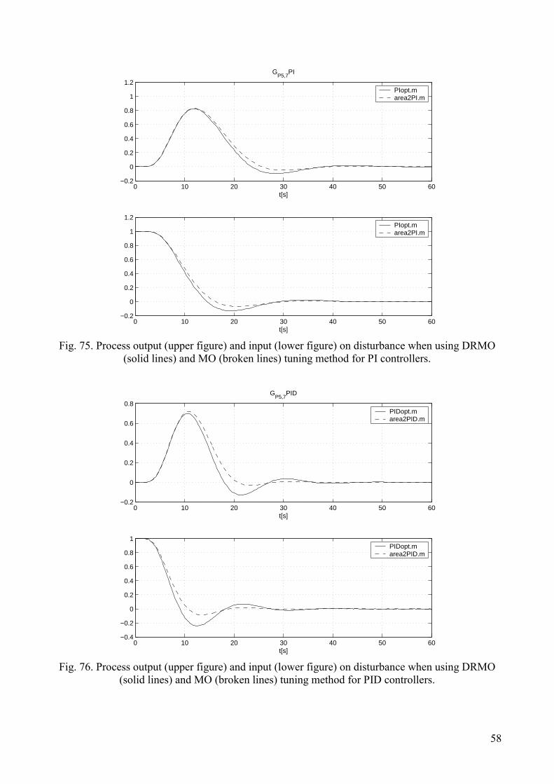
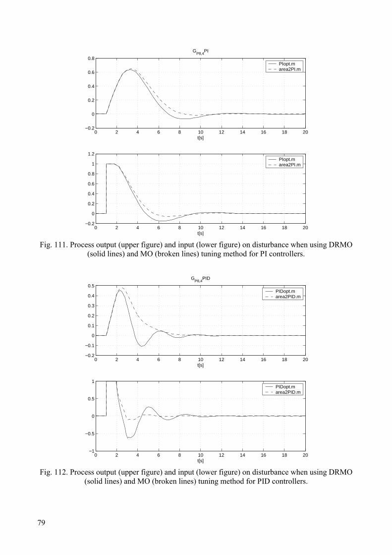
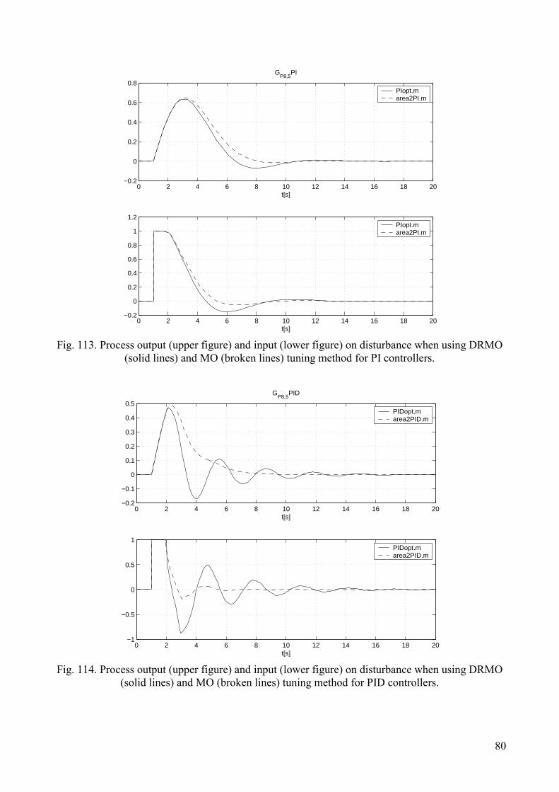
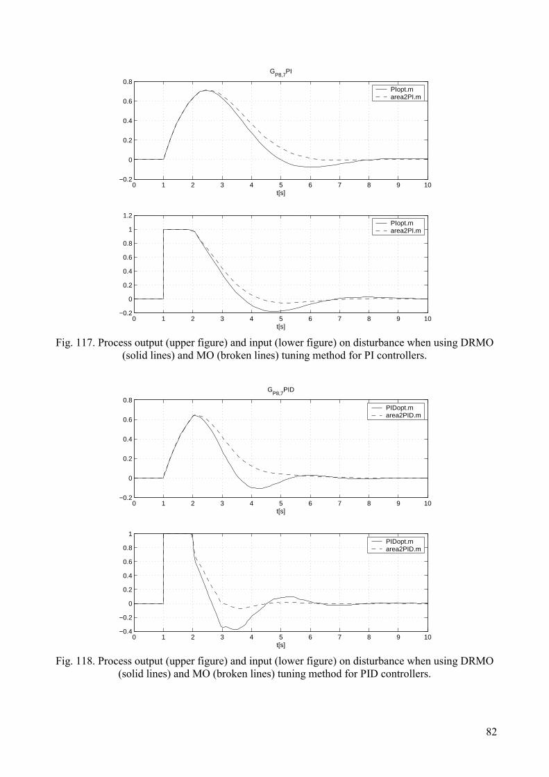
The PI and PID controller parameters, calculated by using the MO method ((9) and (8)), are denoted as “area2PI” and “area2PID”, respectively (matlab functions area2PI.m and are2PID.m are given in Appendix B). The PI and PID controller parameters calculated by using the DRMO method are denoted as “PIopt” and “PIDopt” (functions PIopt.m and PIDopt.m are given in Appendix B). Indexes in GPi,j denote i = process (1-9), j = sub-process (1-7).
19
Process 1: 11 +
=−
TseG
s
P
Table 1. PI controller parameters calculated by using DRMO method (PIopt.m)
T 0.1 0.2 0.5 1 2 5 10
K 0.27529 0.2946 0.39546 0.62772 1.1643 2.8814 5.7944
Ki 0.73925 0.69833 0.6491 0.66237 0.78073 1.2555 2.0984
Table 2. PI controller parameters calculated by using MO method (area2PI.m)
T 0.1 0.2 0.5 1 2 5 10
K 0.25677 0.27442 0.36538 0.57143 1.0395 2.5165 5.0083
Ki 0.68797 0.64535 0.57692 0.53571 0.51316 0.50275 0.50076
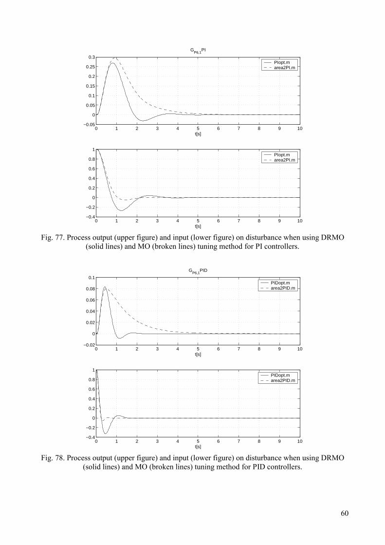
Table 3. PID controller parameters calculated by using DRMO method (PIDopt.m)
T 0.1 0.2 0.5 1 2 5 10
K 0.52017 0.57028 0.80817 1.3081 2.3983 5.7799 10
Ki 0.97611 0.94752 0.97649 1.1468 1.5836 3.0034 4.4475
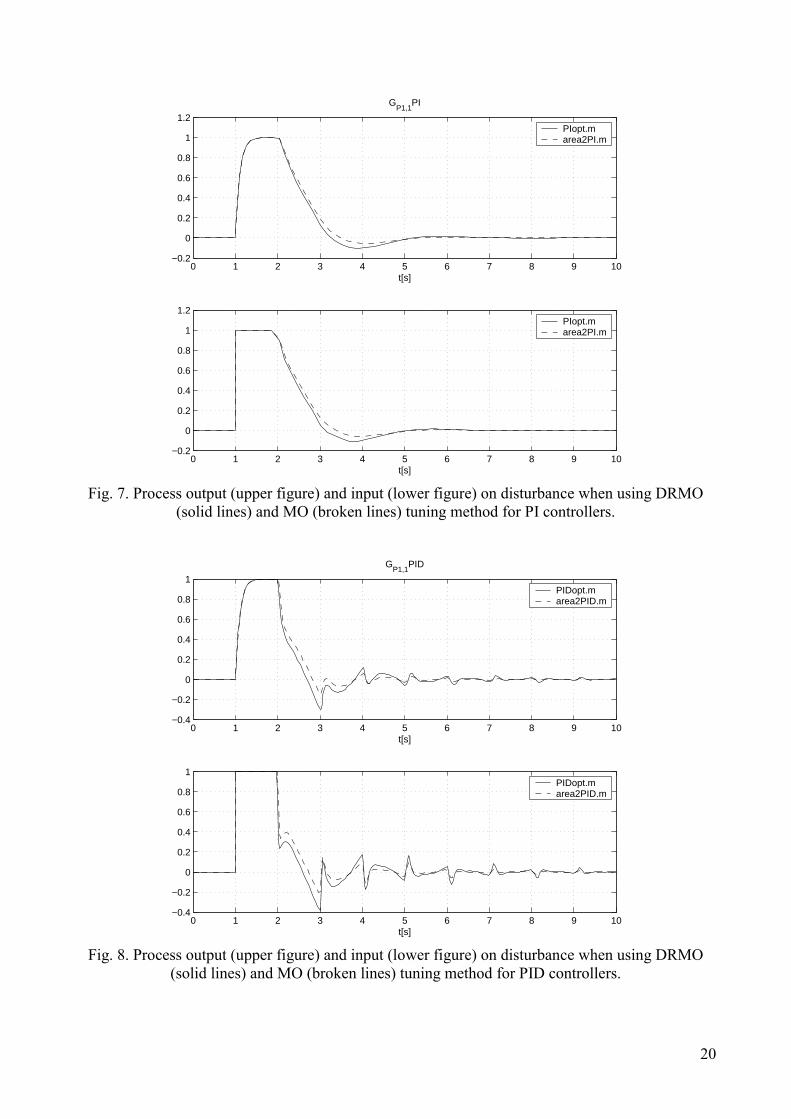
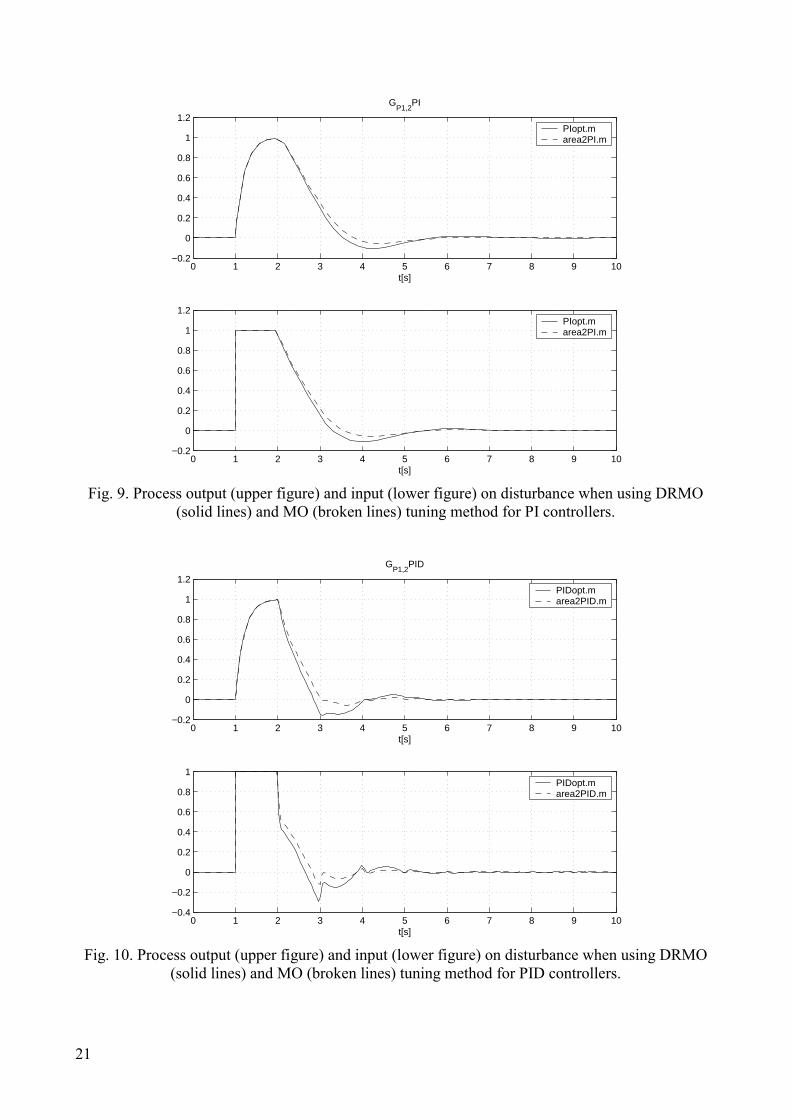
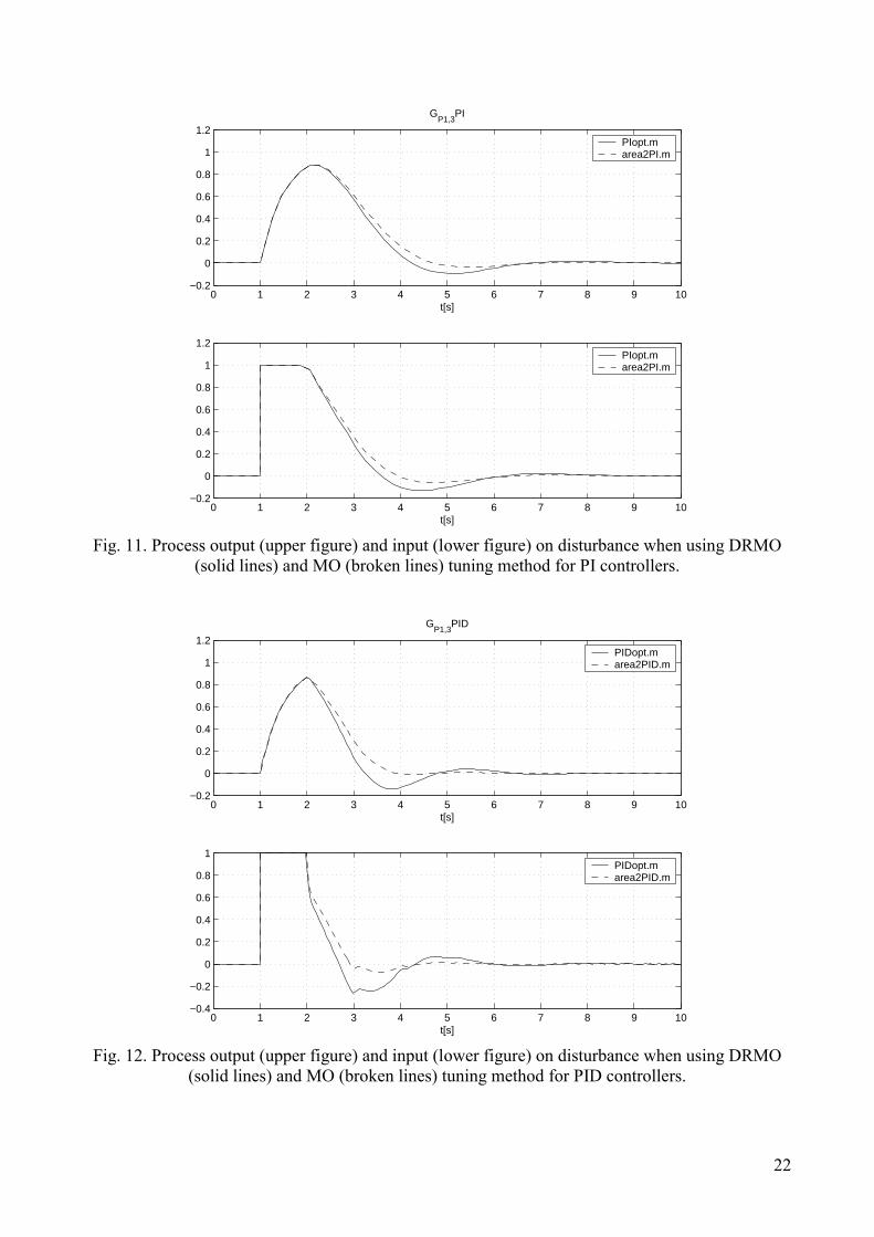
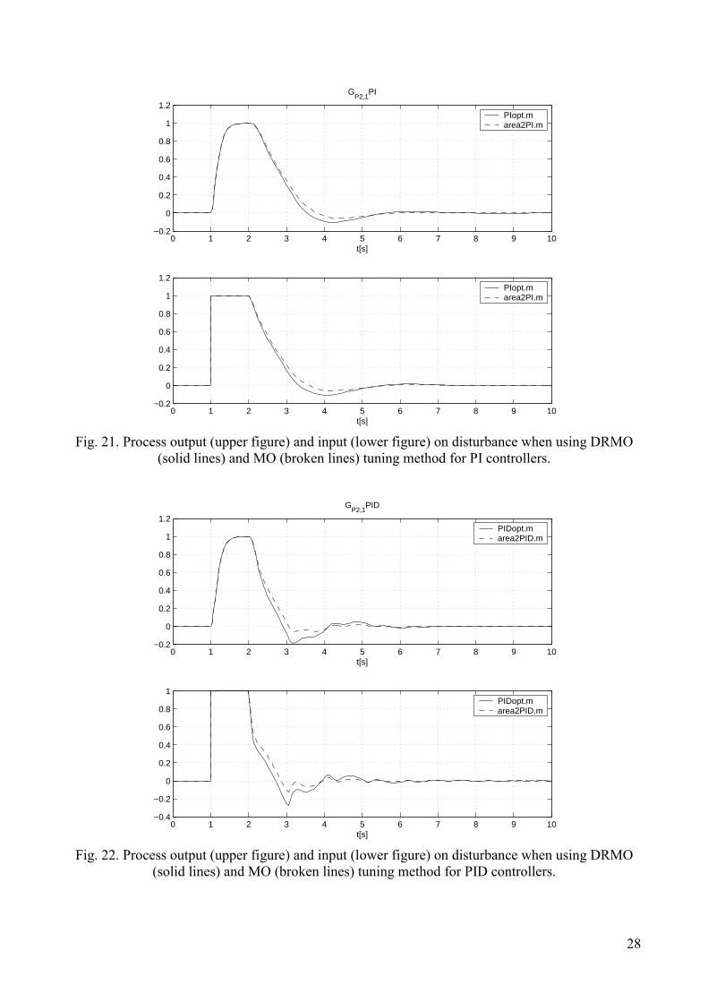
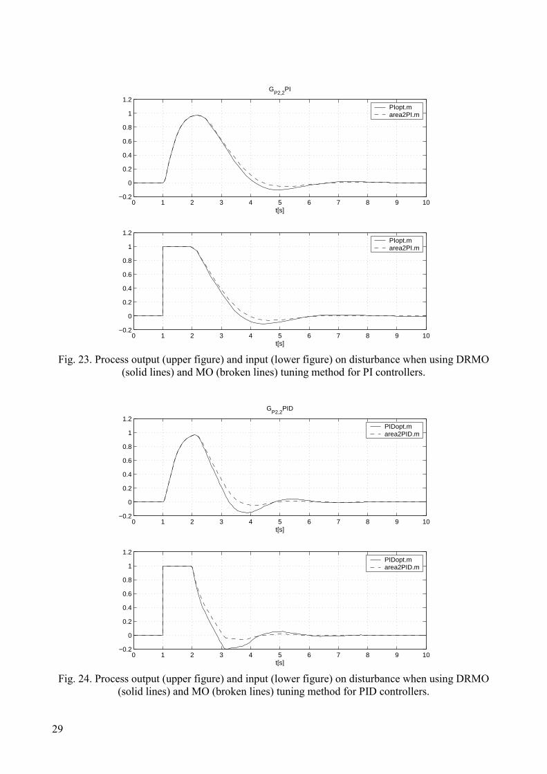
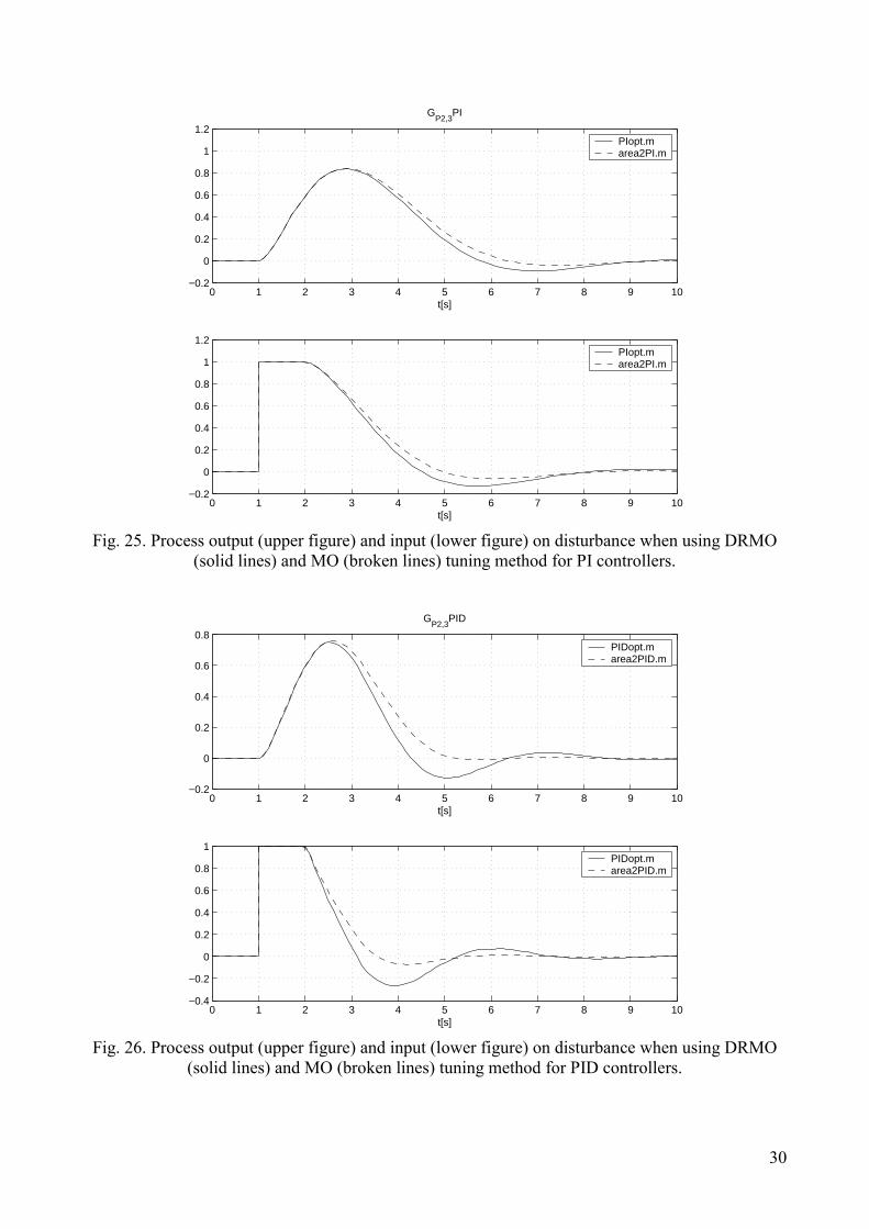
Fig. 105. Process output (upper figure) and input (lower figure) on disturbance when using DRMO
(solid lines) and MO (broken lines) tuning method for PI controllers.
0 2 4 6 8 10 12 14 16 18 20−0.1
0
0.1
0.2
0.3
0.4
0.5
0.6
t[s]
GP8,1
PID
PIDopt.m area2PID.m
0 2 4 6 8 10 12 14 16 18 20−0.4
−0.2
0
0.2
0.4
0.6
0.8
1
t[s]
PIDopt.m area2PID.m
Fig. 106. Process output (upper figure) and input (lower figure) on disturbance when using DRMO
(solid lines) and MO (broken lines) tuning method for PID controllers.
77
0 2 4 6 8 10 12 14 16 18 20−0.2
0
0.2
0.4
0.6
0.8
t[s]
GP8,2
PI
PIopt.m area2PI.m
0 2 4 6 8 10 12 14 16 18 20−0.2
0
0.2
0.4
0.6
0.8
1
1.2
t[s]
PIopt.m area2PI.m
Fig. 107. Process output (upper figure) and input (lower figure) on disturbance when using DRMO
(solid lines) and MO (broken lines) tuning method for PI controllers.
0 2 4 6 8 10 12 14 16 18 20−0.1
0
0.1
0.2
0.3
0.4
0.5
0.6
t[s]
GP8,2
PID
PIDopt.m area2PID.m
0 2 4 6 8 10 12 14 16 18 20−0.5
0
0.5
1
t[s]
PIDopt.m area2PID.m
Fig. 108. Process output (upper figure) and input (lower figure) on disturbance when using DRMO
(solid lines) and MO (broken lines) tuning method for PID controllers.
78
0 2 4 6 8 10 12 14 16 18 20−0.2
0
0.2
0.4
0.6
0.8
t[s]
GP8,3
PI
PIopt.m area2PI.m
0 2 4 6 8 10 12 14 16 18 20−0.2
0
0.2
0.4
0.6
0.8
1
1.2
t[s]
PIopt.m area2PI.m
Fig. 109. Process output (upper figure) and input (lower figure) on disturbance when using DRMO
(solid lines) and MO (broken lines) tuning method for PI controllers.
0 2 4 6 8 10 12 14 16 18 20−0.1
0
0.1
0.2
0.3
0.4
0.5
0.6
t[s]
GP8,3
PID
PIDopt.m area2PID.m
0 2 4 6 8 10 12 14 16 18 20−1
−0.5
0
0.5
1
t[s]
PIDopt.m area2PID.m
Fig. 110. Process output (upper figure) and input (lower figure) on disturbance when using DRMO
(solid lines) and MO (broken lines) tuning method for PID controllers.
79
0 2 4 6 8 10 12 14 16 18 20−0.2
0
0.2
0.4
0.6
0.8
t[s]
GP8,4
PI
PIopt.m area2PI.m
0 2 4 6 8 10 12 14 16 18 20−0.2
0
0.2
0.4
0.6
0.8
1
1.2
t[s]
PIopt.m area2PI.m
Fig. 111. Process output (upper figure) and input (lower figure) on disturbance when using DRMO
(solid lines) and MO (broken lines) tuning method for PI controllers.
0 2 4 6 8 10 12 14 16 18 20−0.2
−0.1
0
0.1
0.2
0.3
0.4
0.5
t[s]
GP8,4
PID
PIDopt.m area2PID.m
0 2 4 6 8 10 12 14 16 18 20−1
−0.5
0
0.5
1
t[s]
PIDopt.m area2PID.m
Fig. 112. Process output (upper figure) and input (lower figure) on disturbance when using DRMO
(solid lines) and MO (broken lines) tuning method for PID controllers.
80
0 2 4 6 8 10 12 14 16 18 20−0.2
0
0.2
0.4
0.6
0.8
t[s]
GP8,5
PI
PIopt.m area2PI.m
0 2 4 6 8 10 12 14 16 18 20−0.2
0
0.2
0.4
0.6
0.8
1
1.2
t[s]
PIopt.m area2PI.m
Fig. 113. Process output (upper figure) and input (lower figure) on disturbance when using DRMO
(solid lines) and MO (broken lines) tuning method for PI controllers.
0 2 4 6 8 10 12 14 16 18 20−0.2
−0.1
0
0.1
0.2
0.3
0.4
0.5
t[s]
GP8,5
PID
PIDopt.m area2PID.m
0 2 4 6 8 10 12 14 16 18 20−1
−0.5
0
0.5
1
t[s]
PIDopt.m area2PID.m
Fig. 114. Process output (upper figure) and input (lower figure) on disturbance when using DRMO
(solid lines) and MO (broken lines) tuning method for PID controllers.
81
0 1 2 3 4 5 6 7 8 9 10−0.2
0
0.2
0.4
0.6
0.8
t[s]
GP8,6
PI
PIopt.m area2PI.m
0 1 2 3 4 5 6 7 8 9 10−0.2
0
0.2
0.4
0.6
0.8
1
1.2
t[s]
PIopt.m area2PI.m
Fig. 115. Process output (upper figure) and input (lower figure) on disturbance when using DRMO
(solid lines) and MO (broken lines) tuning method for PI controllers.
0 1 2 3 4 5 6 7 8 9 10−0.4
−0.2
0
0.2
0.4
0.6
t[s]
GP8,6
PID
PIDopt.m area2PID.m
0 1 2 3 4 5 6 7 8 9 10−1.5
−1
−0.5
0
0.5
1
t[s]
PIDopt.m area2PID.m
Fig. 116. Process output (upper figure) and input (lower figure) on disturbance when using DRMO
(solid lines) and MO (broken lines) tuning method for PID controllers.
82
0 1 2 3 4 5 6 7 8 9 10−0.2
0
0.2
0.4
0.6
0.8
t[s]
GP8,7
PI
PIopt.m area2PI.m
0 1 2 3 4 5 6 7 8 9 10−0.2
0
0.2
0.4
0.6
0.8
1
1.2
t[s]
PIopt.m area2PI.m
Fig. 117. Process output (upper figure) and input (lower figure) on disturbance when using DRMO
(solid lines) and MO (broken lines) tuning method for PI controllers.
0 1 2 3 4 5 6 7 8 9 10−0.2
0
0.2
0.4
0.6
0.8
t[s]
GP8,7
PID
PIDopt.m area2PID.m
0 1 2 3 4 5 6 7 8 9 10−0.4
−0.2
0
0.2
0.4
0.6
0.8
1
t[s]
PIDopt.m area2PID.m
Fig. 118. Process output (upper figure) and input (lower figure) on disturbance when using DRMO
(solid lines) and MO (broken lines) tuning method for PID controllers.
83
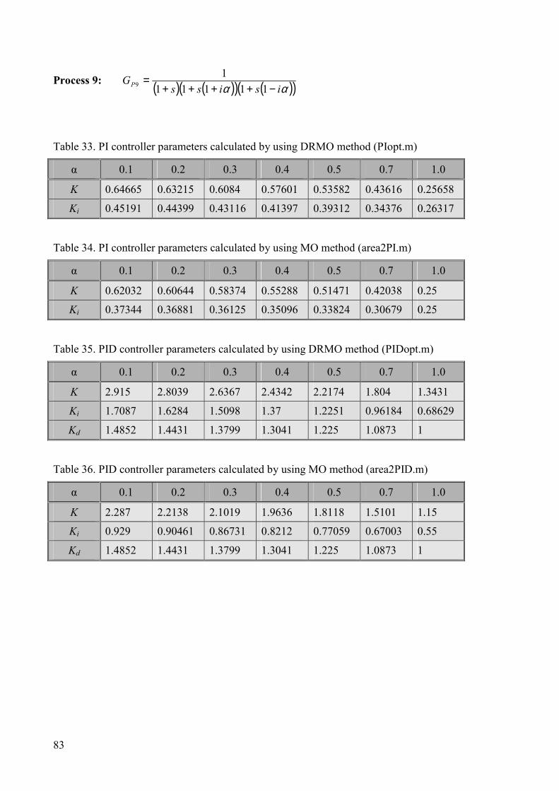
Process 9: ( ) ( )( ) ( )( )αα isissGP −++++
=11111
19
Table 33. PI controller parameters calculated by using DRMO method (PIopt.m)
α 0.1 0.2 0.3 0.4 0.5 0.7 1.0
K 0.64665 0.63215 0.6084 0.57601 0.53582 0.43616 0.25658
Ki 0.45191 0.44399 0.43116 0.41397 0.39312 0.34376 0.26317
Table 34. PI controller parameters calculated by using MO method (area2PI.m)
α 0.1 0.2 0.3 0.4 0.5 0.7 1.0
K 0.62032 0.60644 0.58374 0.55288 0.51471 0.42038 0.25
Ki 0.37344 0.36881 0.36125 0.35096 0.33824 0.30679 0.25
Table 35. PID controller parameters calculated by using DRMO method (PIDopt.m)
α 0.1 0.2 0.3 0.4 0.5 0.7 1.0
K 2.915 2.8039 2.6367 2.4342 2.2174 1.804 1.3431
Ki 1.7087 1.6284 1.5098 1.37 1.2251 0.96184 0.68629
Kd 1.4852 1.4431 1.3799 1.3041 1.225 1.0873 1
Table 36. PID controller parameters calculated by using MO method (area2PID.m)
α 0.1 0.2 0.3 0.4 0.5 0.7 1.0
K 2.287 2.2138 2.1019 1.9636 1.8118 1.5101 1.15
Ki 0.929 0.90461 0.86731 0.8212 0.77059 0.67003 0.55
Kd 1.4852 1.4431 1.3799 1.3041 1.225 1.0873 1
84
0 2 4 6 8 10 12 14 16 18 20−0.1
0
0.1
0.2
0.3
0.4
0.5
0.6
t[s]
GP9,1
PI
PIopt.m area2PI.m
0 2 4 6 8 10 12 14 16 18 20−0.2
0
0.2
0.4
0.6
0.8
1
1.2
t[s]
PIopt.m area2PI.m
Fig. 119. Process output (upper figure) and input (lower figure) on disturbance when using DRMO
(solid lines) and MO (broken lines) tuning method for PI controllers.
0 2 4 6 8 10 12 14 16 18 20−0.05
0
0.05
0.1
0.15
0.2
0.25
0.3
t[s]
GP9,1
PID
PIDopt.m area2PID.m
0 2 4 6 8 10 12 14 16 18 20−0.4
−0.2
0
0.2
0.4
0.6
0.8
1
t[s]
PIDopt.m area2PID.m
Fig. 120. Process output (upper figure) and input (lower figure) on disturbance when using DRMO
(solid lines) and MO (broken lines) tuning method for PID controllers.
85
0 2 4 6 8 10 12 14 16 18 20−0.1
0
0.1
0.2
0.3
0.4
0.5
0.6
t[s]
GP9,2
PI
PIopt.m area2PI.m
0 2 4 6 8 10 12 14 16 18 20−0.2
0
0.2
0.4
0.6
0.8
1
1.2
t[s]
PIopt.m area2PI.m
Fig. 121. Process output (upper figure) and input (lower figure) on disturbance when using DRMO
(solid lines) and MO (broken lines) tuning method for PI controllers.
0 2 4 6 8 10 12 14 16 18 20−0.05
0
0.05
0.1
0.15
0.2
0.25
0.3
t[s]
GP9,2
PID
PIDopt.m area2PID.m
0 2 4 6 8 10 12 14 16 18 20−0.4
−0.2
0
0.2
0.4
0.6
0.8
1
t[s]
PIDopt.m area2PID.m
Fig. 122. Process output (upper figure) and input (lower figure) on disturbance when using DRMO
(solid lines) and MO (broken lines) tuning method for PID controllers.
86
0 2 4 6 8 10 12 14 16 18 20−0.1
0
0.1
0.2
0.3
0.4
0.5
0.6
t[s]
GP9,3
PI
PIopt.m area2PI.m
0 2 4 6 8 10 12 14 16 18 20−0.2
0
0.2
0.4
0.6
0.8
1
1.2
t[s]
PIopt.m area2PI.m
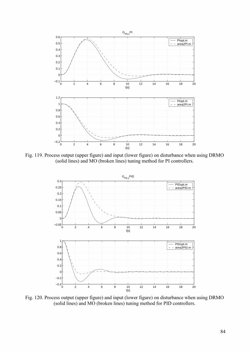
Fig. 123. Process output (upper figure) and input (lower figure) on disturbance when using DRMO
(solid lines) and MO (broken lines) tuning method for PI controllers.
0 2 4 6 8 10 12 14 16 18 20−0.1
0
0.1
0.2
0.3
0.4
t[s]
GP9,3
PID
PIDopt.m area2PID.m
0 2 4 6 8 10 12 14 16 18 20−0.4
−0.2
0
0.2
0.4
0.6
0.8
1
t[s]
PIDopt.m area2PID.m
Fig. 124. Process output (upper figure) and input (lower figure) on disturbance when using DRMO
(solid lines) and MO (broken lines) tuning method for PID controllers.
87
0 2 4 6 8 10 12 14 16 18 20−0.2
0
0.2
0.4
0.6
0.8
t[s]
GP9,4
PI
PIopt.m area2PI.m
0 2 4 6 8 10 12 14 16 18 20−0.2
0
0.2
0.4
0.6
0.8
1
1.2
t[s]
PIopt.m area2PI.m
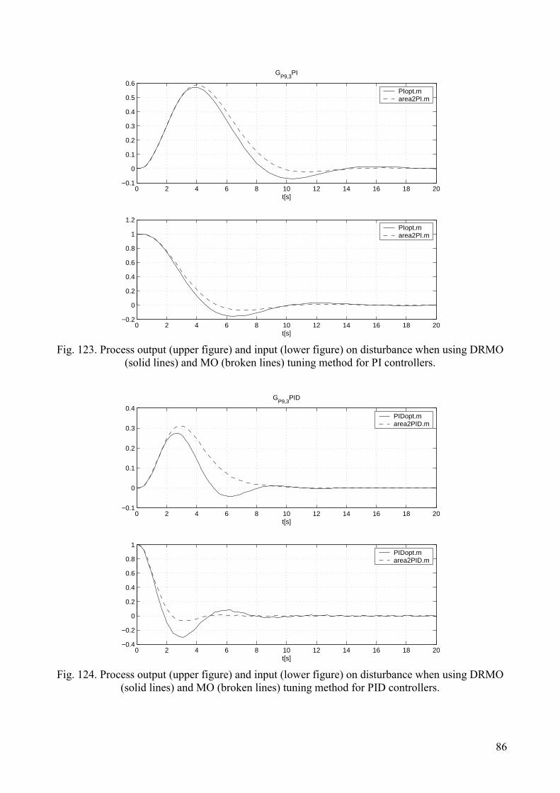
Fig. 125. Process output (upper figure) and input (lower figure) on disturbance when using DRMO
(solid lines) and MO (broken lines) tuning method for PI controllers.
0 2 4 6 8 10 12 14 16 18 20−0.1
0
0.1
0.2
0.3
0.4
t[s]
GP9,4
PID
PIDopt.m area2PID.m
0 2 4 6 8 10 12 14 16 18 20−0.4
−0.2
0
0.2
0.4
0.6
0.8
1
t[s]
PIDopt.m area2PID.m
Fig. 126. Process output (upper figure) and input (lower figure) on disturbance when using DRMO
(solid lines) and MO (broken lines) tuning method for PID controllers.
88
0 2 4 6 8 10 12 14 16 18 20−0.2
0
0.2
0.4
0.6
0.8
t[s]
GP9,5
PI
PIopt.m area2PI.m
0 2 4 6 8 10 12 14 16 18 20−0.2
0
0.2
0.4
0.6
0.8
1
1.2
t[s]
PIopt.m area2PI.m
Fig. 127. Process output (upper figure) and input (lower figure) on disturbance when using DRMO
(solid lines) and MO (broken lines) tuning method for PI controllers.
0 2 4 6 8 10 12 14 16 18 20−0.1
0
0.1
0.2
0.3
0.4
t[s]
GP9,5
PID
PIDopt.m area2PID.m
0 2 4 6 8 10 12 14 16 18 20−0.4
−0.2
0
0.2
0.4
0.6
0.8
1
t[s]
PIDopt.m area2PID.m
Fig. 128. Process output (upper figure) and input (lower figure) on disturbance when using DRMO
(solid lines) and MO (broken lines) tuning method for PID controllers.
89
0 2 4 6 8 10 12 14 16 18 20−0.2
0
0.2
0.4
0.6
0.8
t[s]
GP9,6
PI
PIopt.m area2PI.m
0 2 4 6 8 10 12 14 16 18 20−0.2
0
0.2
0.4
0.6
0.8
1
1.2
t[s]
PIopt.m area2PI.m
Fig. 129. Process output (upper figure) and input (lower figure) on disturbance when using DRMO
(solid lines) and MO (broken lines) tuning method for PI controllers.
0 2 4 6 8 10 12 14 16 18 20−0.1
0
0.1
0.2
0.3
0.4
t[s]
GP9,6
PID
PIDopt.m area2PID.m
0 2 4 6 8 10 12 14 16 18 20−0.4
−0.2
0
0.2
0.4
0.6
0.8
1
t[s]
PIDopt.m area2PID.m
Fig. 130. Process output (upper figure) and input (lower figure) on disturbance when using DRMO
(solid lines) and MO (broken lines) tuning method for PID controllers.
90
0 2 4 6 8 10 12 14 16 18 20−0.2
0
0.2
0.4
0.6
0.8
t[s]
GP9,7
PI
PIopt.m area2PI.m
0 2 4 6 8 10 12 14 16 18 20−0.2
0
0.2
0.4
0.6
0.8
1
1.2
t[s]
PIopt.m area2PI.m
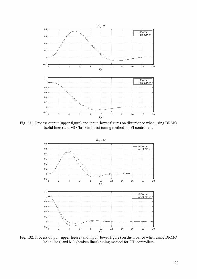
Fig. 131. Process output (upper figure) and input (lower figure) on disturbance when using DRMO
(solid lines) and MO (broken lines) tuning method for PI controllers.
0 2 4 6 8 10 12 14 16 18 20−0.1
0
0.1
0.2
0.3
0.4
0.5
0.6
t[s]
GP9,7
PID
PIDopt.m area2PID.m
0 2 4 6 8 10 12 14 16 18 20−0.2
0
0.2
0.4
0.6
0.8
1
1.2
t[s]
PIDopt.m area2PID.m
Fig. 132. Process output (upper figure) and input (lower figure) on disturbance when using DRMO
(solid lines) and MO (broken lines) tuning method for PID controllers.
91
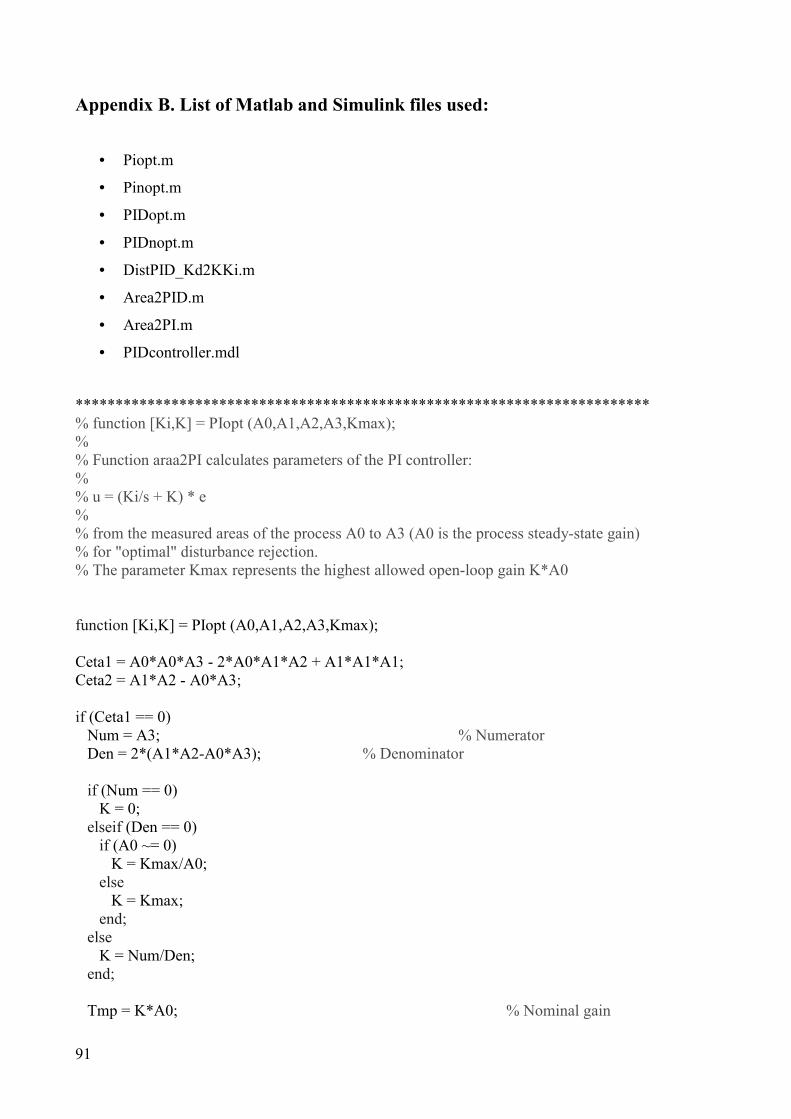
Appendix B. List of Matlab and Simulink files used:
• Piopt.m
• Pinopt.m
• PIDopt.m
• PIDnopt.m
• DistPID_Kd2KKi.m
• Area2PID.m
• Area2PI.m
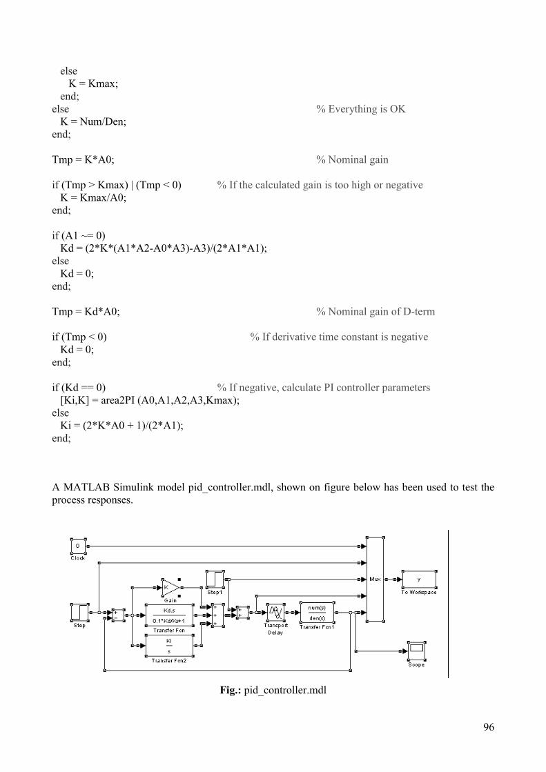
• PIDcontroller.mdl
************************************************************************ % function [Ki,K] = PIopt (A0,A1,A2,A3,Kmax); % % Function araa2PI calculates parameters of the PI controller: % % u = (Ki/s + K) * e % % from the measured areas of the process A0 to A3 (A0 is the process steady-state gain) % for "optimal" disturbance rejection. % The parameter Kmax represents the highest allowed open-loop gain K*A0 function [Ki,K] = PIopt (A0,A1,A2,A3,Kmax); Ceta1 = A0*A0*A3 - 2*A0*A1*A2 + A1*A1*A1; Ceta2 = A1*A2 - A0*A3; if (Ceta1 == 0) Num = A3; % Numerator Den = 2*(A1*A2-A0*A3); % Denominator if (Num == 0) K = 0; elseif (Den == 0) if (A0 ~= 0) K = Kmax/A0; else K = Kmax; end; else K = Num/Den; end; Tmp = K*A0; % Nominal gain
92
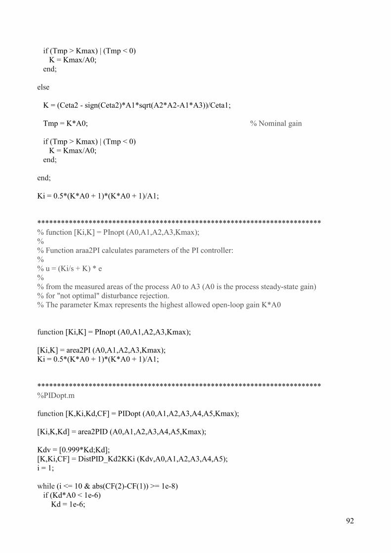
if (Tmp > Kmax) | (Tmp < 0) K = Kmax/A0; end; else K = (Ceta2 - sign(Ceta2)*A1*sqrt(A2*A2-A1*A3))/Ceta1; Tmp = K*A0; % Nominal gain if (Tmp > Kmax) | (Tmp < 0) K = Kmax/A0; end; end; Ki = 0.5*(K*A0 + 1)*(K*A0 + 1)/A1; ************************************************************************ % function [Ki,K] = PInopt (A0,A1,A2,A3,Kmax); % % Function araa2PI calculates parameters of the PI controller: % % u = (Ki/s + K) * e % % from the measured areas of the process A0 to A3 (A0 is the process steady-state gain) % for "not optimal" disturbance rejection. % The parameter Kmax represents the highest allowed open-loop gain K*A0 function [Ki,K] = PInopt (A0,A1,A2,A3,Kmax); [Ki,K] = area2PI (A0,A1,A2,A3,Kmax); Ki = 0.5*(K*A0 + 1)*(K*A0 + 1)/A1; ************************************************************************ %PIDopt.m function [K,Ki,Kd,CF] = PIDopt (A0,A1,A2,A3,A4,A5,Kmax); [Ki,K,Kd] = area2PID (A0,A1,A2,A3,A4,A5,Kmax); Kdv = [0.999*Kd;Kd]; [K,Ki,CF] = DistPID_Kd2KKi (Kdv,A0,A1,A2,A3,A4,A5); i = 1; while (i <= 10 & abs(CF(2)-CF(1)) >= 1e-8) if (Kd*A0 < 1e-6) Kd = 1e-6;
93
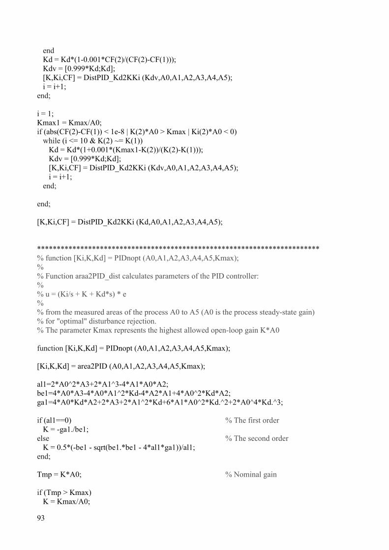
end Kd = Kd*(1-0.001*CF(2)/(CF(2)-CF(1))); Kdv = [0.999*Kd;Kd]; [K,Ki,CF] = DistPID_Kd2KKi (Kdv,A0,A1,A2,A3,A4,A5); i = i+1; end; i = 1; Kmax1 = Kmax/A0; if (abs(CF(2)-CF(1)) < 1e-8 | K(2)*A0 > Kmax | Ki(2)*A0 < 0) while (i <= 10 & K(2) ~= K(1)) Kd = Kd*(1+0.001*(Kmax1-K(2))/(K(2)-K(1))); Kdv = [0.999*Kd;Kd]; [K,Ki,CF] = DistPID_Kd2KKi (Kdv,A0,A1,A2,A3,A4,A5); i = i+1; end; end; [K,Ki,CF] = DistPID_Kd2KKi (Kd,A0,A1,A2,A3,A4,A5); ************************************************************************ % function [Ki,K,Kd] = PIDnopt (A0,A1,A2,A3,A4,A5,Kmax); % % Function araa2PID_dist calculates parameters of the PID controller: % % u = (Ki/s + K + Kd*s) * e % % from the measured areas of the process A0 to A5 (A0 is the process steady-state gain) % for "optimal" disturbance rejection. % The parameter Kmax represents the highest allowed open-loop gain K*A0 function [Ki,K,Kd] = PIDnopt (A0,A1,A2,A3,A4,A5,Kmax); [Ki,K,Kd] = area2PID (A0,A1,A2,A3,A4,A5,Kmax); al1=2*A0^2*A3+2*A1^3-4*A1*A0*A2; be1=4*A0*A3-4*A0*A1^2*Kd-4*A2*A1+4*A0^2*Kd*A2; ga1=4*A0*Kd*A2+2*A3+2*A1^2*Kd+6*A1*A0^2*Kd.^2+2*A0^4*Kd.^3; if (al1==0) % The first order K = -ga1./be1; else % The second order K = 0.5*(-be1 - sqrt(be1.*be1 - 4*al1*ga1))/al1; end; Tmp = K*A0; % Nominal gain if (Tmp > Kmax) K = Kmax/A0;
94
Kdv = [0.999*Kd;Kd]; [Kv,Kiv,CF] = DistPID_Kd2KKi (Kdv,A0,A1,A2,A3,A4,A5); i = 1; Kmax1 = Kmax/A0; while (i <= 10 & Kv(2) ~= Kv(1)) Kd = Kd*(1+0.001*(Kmax1-Kv(2))/(Kv(2)-Kv(1))); Kdv = [0.999*Kd;Kd]; [Kv,Kiv,CF] = DistPID_Kd2KKi (Kdv,A0,A1,A2,A3,A4,A5); i = i+1; end; K = Kv(2); elseif (Tmp < 0) K = 0; end; Ki = 0.5*(1 + 2*A0*K + A0^2*K^2)/(A1 + A0^2*Kd); if (Ki*A0 < 0) Ki = 0; end; ************************************************************************ %DistPID_Kd2KKi.m function [K,Ki,CF] = DistPID_Kd2KKi (Kd,A0,A1,A2,A3,A4,A5); al1=2*A0^2*A3+2*A1^3-4*A1*A0*A2; be1=4*A0*A3-4*A0*A1^2*Kd-4*A2*A1+4*A0^2*Kd*A2; ga1=4*A0*Kd*A2+2*A3+2*A1^2*Kd+6*A1*A0^2*Kd.^2+2*A0^4*Kd.^3; if (al1==0) % The first order K = -ga1./be1; else % The second order K = 0.5*(-be1 - sqrt(be1.*be1 - 4*al1*ga1))/al1; end; Ki = 0.5*(1+2*A0*K+A0^2*K.^2)./(A1+A0^2*Kd); CF = -4*A0*Ki*A4.*Kd-2*A3*Kd+2*A4*K-2*A5*Ki+2*A0*K.^2*A4-2*A0*Kd.^2*A2-2*A1*K.^2*A3-2*A2^2*Ki.*Kd+A1^2*Kd.^2+A2^2*K.^2+4*A1*Kd*A3.*Ki; ************************************************************************ % function [Ki,K] = area2PI (A0,A1,A2,A3,Kmax); % % Function araa2PI calculates parameters of the PI controller: % % u = (Ki/s + K) * e %
95
% from the measured areas of the process A0 to A3 (A0 is the process steady-state gain) % The parameter Kmax represents the highest allowed open-loop gain K*A0 function [Ki,K] = area2PI (A0,A1,A2,A3,Kmax); Num = A3; % Numerator Den = 2*(A1*A2-A0*A3); % Denominator if (Num == 0) K = 0; elseif (Den == 0) if (A0 ~= 0) K = Kmax/A0; else K = Kmax; end; else K = Num/Den; end; Tmp = K*A0; % Nominal gain if (Tmp > Kmax) | (Tmp < 0) K = Kmax/A0; end; Ki = (K*A0 + 0.5)/A1; ************************************************************************ % function [Ki,K,Kd] = area2PID (A0,A1,A2,A3,A4,A5,Kmax); % % Function araa2PID calculates parameters of the PID controller: % % u = (Ki/s + K + Kd*s) * e % % from the measured areas of the process A0 to A5 (A0 is the process steady-state gain) % The parameter Kmax represents the highest allowed open-loop gain K*A0 function [Ki,K,Kd] = area2PID (A0,A1,A2,A3,A4,A5,Kmax); Num = A3*A3 - A1*A5; % Numerator Den = 2*(A1*A2*A3+A0*A1*A5-A1*A1*A4-A0*A3*A3); % Denominator if (Num == 0) K = 0; elseif (Den == 0) % Division with zero if (A0 ~= 0) K = Kmax/A0;
96
else K = Kmax; end; else % Everything is OK K = Num/Den; end; Tmp = K*A0; % Nominal gain if (Tmp > Kmax) | (Tmp < 0) % If the calculated gain is too high or negative K = Kmax/A0; end; if (A1 ~= 0) Kd = (2*K*(A1*A2-A0*A3)-A3)/(2*A1*A1); else Kd = 0; end; Tmp = Kd*A0; % Nominal gain of D-term if (Tmp < 0) % If derivative time constant is negative Kd = 0; end; if (Kd == 0) % If negative, calculate PI controller parameters [Ki,K] = area2PI (A0,A1,A2,A3,Kmax); else Ki = (2*K*A0 + 1)/(2*A1); end;
A MATLAB Simulink model pid_controller.mdl, shown on figure below has been used to test the process responses.