Proceedings of the AREMA 2006 Annual Conference, Louisville, KY (September 2006)

Improving Railroad Classification Yard Performance Through Bottleneck Management Methods

Jeremiah R. Dirnberger

Graduate Research Assistant Railroad Engineering Program

Department of Civil and Environmental Engineering University of Illinois at Urbana-Champaign

B-118 Newmark Civil Engineering Laboratory 205 N. Matthews Ave., Urbana, IL 61801

Tel: (217) 244-6063 Fax: (217) 333-1924 dirnbrgr@uiuc.edu

Current Address:

Specialist, Yard Operations Performance Canadian Pacific Railway

Gulf Canada Square, 401 – 9th Ave SW Calgary, AB T2P 4Z4 Tel: (403) 319-3810

jeremiah_dirnberger@cpr.ca

Christopher P.L. Barkan Associate Professor

George Krambles Faculty Fellow Director - Railroad Engineering Program

Department of Civil and Environmental Engineering University of Illinois at Urbana-Champaign

1201 Newmark Civil Engineering Laboratory 205 N. Matthews Ave., Urbana, IL 61801

Tel: (217) 244-6338 Fax: (217) 333-1924 cbarkan@uiuc.edu

Abstract: 249 words Body: 5,258 words + 5 Figures (1,250 words) + 2 Tables (500 words) = 7,008 words

ABSTRACT

Because railroad classification yards can be considered production systems, insight into the

dynamics of a yard system can be gained by adapting production management tools that have led

to significant performance improvement in manufacturing. This work focused on improving

yard performance by utilizing the concepts of factory physics, Theory of Constraints (TOC) and

tools from Lean Manufacturing.

The most important manufacturing process analog to improving yard capacity is the

bottleneck. In a production system the bottleneck is the process that limits its throughput. As

such, the processing rate of the bottleneck sets the rate for the entire system. Improving the

performance of the bottleneck is the best way to improve the performance of the entire terminal

process. The train assembly (pull-down) process has been identified as the bottleneck in a

majority of classification yards. The potential capacity improvement of several bottleneck

management alternatives is discussed.

One of the principal findings of this work is that the humping process should be

subordinate to the pull-down process because the latter is the principal bottleneck in many yards.

The hump should be managed and operated so that it provides the bottleneck exactly what it

needs when it needs it. The quality of sorting during hump operation directly affects the

performance of the pull-down process. A metric for measuring how well during cars in the

classification yard have been sorted has been developed and its relationship to yard volume

established. Methods for implementing this metric in a classification yard are also discussed.

INTRODUCTION

While shipping by railroad is usually less expensive than trucking, the lower level of service

reliability can produce higher total logistical costs for shippers and receivers. Higher variability

in shipment arrival times results in additional inventory having to be carried in order for a

railroad customer to maintain a fixed level of customer service (1). Previous studies have

established the need for the railroad industry to improve service reliability in order to meet the

increasing logistical demands of shippers (2). These same studies have named the classification

yard as a key determinant in the service reliability of general manifest (or carload) freight. The

trade off between high cost efficiency and reduced service quality is inherent to carload railroad

operations. For railroads to continue to grow their business, they must work to overcome the

tradeoff.

A majority of total trip cycle time is spent in yards. Two major North American railroads

have reported that 59% (3) and 64% (Figure 1) of railcar transit time is spent in yards. “This

suggests that the reliability of car movements can be improved by reducing the time spent in

those activities or by making them more reliable” (4). The transition to scheduled operations by

all of North America’s Class I railroads has increased the interaction between yard performance

and service reliability (5, 6) because “efficient high-throughput classification yards are vital to

scheduled railroading” (7).

Within a classification yard, connections are made by classifying cars from inbound

trains into blocks that will be assembled into outbound trains. The objective is to sort cars and

reliably connect them to the earliest possible candidate outbound train, while minimizing cost

(Barker unpublished date). Kraft has extensively studied the connection reliability problem as it

relates to dynamic car scheduling (8) and has developed a hump sequencing algorithm (9), a

priority-based classification system (5) and a dynamic block to track assignment scheme with the

goal of ensuring connections (6). Kraft raises the issue of inadequate terminal capacity as a

barrier to improved service reliability (9). However, the availability of capital and the physical

capability to expand some yards may be constrained. Therefore, in addition to considering

infrastructure expansion, railroads must also determine how to harness as much capacity from

extant infrastructure as possible. This creates the need for new management and operational

methods that will increase the capacity of existing facilities.

Manufacturers face a similar need and this presents the opportunity for the use of selected

techniques from production management. Yard capacity can be improved an estimated 15-30%

(3) by adapting an approach known as “Lean Railroading” (10) with emphasis on the bottleneck

management component. The pull-down process is identified as the most common bottleneck in

hump yards. The macroscopic evaluation method from Wong et al. (11) is enhanced with two

additional equations and used to evaluate several improvement alternatives using Bensenville

Yard (CPR) near Chicago as the example. To aid in implementing one of the more promising

alternatives, a Quality of Sort metric is developed to better manage and understand the

interaction between the pull-down process and its immediate upstream process (the hump).

LEAN RAILROADING

Because classification yards can be considered production systems (12), their performance can

be improved by adapting an integrated approach comprised of three proven production

management techniques: Lean, Theory of Constraints (TOC) and Statistical Process Control

(SPC or “six sigma”). Known as “Lean Railroading” (10), several railroads and railroad

suppliers, including Canadian Pacific (CPR), Union Pacific (UP), BNSF, Norfolk Southern (NS),

the Belt Railway of Chicago and GE Yard Solutions, are actively applying all or parts of this

approach to improving yard performance. In addition, many of the “precision railroading”

principles that CN has used to improve their operating performance can also be considered lean.

The first step in any lean program is to define value for the ultimate customer and then

work to increase value by eliminating waste in the system. Waste is defined as any step or

process in a production system that, from the standpoint of the customer, does not add value to

the product (13). Waste can be classified into two types: direct waste and variability (14).

Direct waste is most easily described as poor railroading practices such as unnecessary moves,

mistakes that require an operation to be repeated, inadequate track maintenance and unsafe

operations to name a few. Focusing on these is important, but the goal of eliminating direct

waste is as old as the railroad itself.

Variability is a fundamentally different source of waste. Hopp & Spearman (1) state, as a

law of manufacturing, that, “Increasing variability always degrades the performance of a

production system.” Railroad yards are no different: they are subject to both internal (i.e.

outages, rework, sorting, etc.) and external (i.e. arrival times, weather, traffic volume, etc.)

sources of variability. Another law of manufacturing from factory physics is “Variability in a

production system will be buffered by some combination of inventory, capacity and time” (1).

In a classification yard, a capacity buffer takes the form of a process throughput greater than the

process demand. A time buffer is the extra time built into each car’s trip plan in order to ensure

that the connection will be made and is seen in the terminal dwell.

Spearman (14) states, “In many ways, the ‘waste’ discussed in Lean is the ‘buffer’ of

Factory Physics. However, this is not always the case. If external variability creates the need for

a buffer, is it waste?” Providing different service levels increases variability, but would the

railroad be better off if it were to only offer one service level? “The point is that while not all

variability is waste, all variability will lead to a buffer which indicates that logistical (but not

necessarily financial) performance has suffered” (14). Therefore, it becomes the task of yard

management to reduce internal variability and the task of network management to manage the

external variability so that the bad sources (like arrival variability) are reduced and the good

sources (like service level differentiation) increase profit.

Implementing Lean Railroading

With the advent of scheduled railroading, railroads have already taken an important first step in

creating an environment that Lean Railroading can succeed in by reducing external variability

for the yard. The implementation steps are:

0. Eliminate direct waste - Take a fresh look at the yard as a system by drawing a Value

Stream Map (VSM) (10, 13) and try to eliminate obvious sources of waste.

1. Swap buffers - Decrease the time buffer (dwell time) by reducing the idle time

between processes. This is synonymous with enabling continuous flow. Increase the

capacity buffer by focusing on improving the performance of the bottleneck.

2. Reduce variability –

a. Address problems in sorting, rework, car damage, down time and setups

(apply SPC/”six sigma”)

b. Implement standardized work plans

c. Work with network management to increase on-time arrival of inbound trains

d. Level the production schedule in the yard and set the network operating plan

3. Continuous improvement – “Once variability is significantly reduced, we can reduce

the capacity buffer while continuing to identify and eliminate variability. Only at this

point do we begin to make real gains in productivity. If we do not reduce variability,

we will not be able to reduce the capacity buffer without hurting customer

responsiveness. The result is a system that continues to improve over time” (14).

The Theoretical Importance of the Bottleneck

In order to decrease the time buffer, without a detrimental impact on connection performance,

the capacity buffer must be increased. Capacity is defined as the upper limit on the throughput

of a production process (1). The bottleneck process limits the throughput of a production

system. As such, the processing rate (throughput) of the bottleneck process establishes the

capacity of the entire system over the long term. Equation 1, Little’s Law (1), can be used to

estimate the benefits of improving the bottleneck rate:

Bottleneck rate = Yard throughput (cars per day) = Volume (car count)Dwell time (days) (1)

Increasing the bottleneck rate will reduce the dwell time for any given volume level in the yard.

Therefore, the avenue for the greatest capacity buffer increase lies with improving the

performance of the bottleneck.

The Theory of Constraints (TOC)

TOC provides a structured approach to improving production system performance by focusing

on the systems’ bottleneck. Goldratt (15) has established the general process in the TOC

approach. For any production system, the TOC approach is:

1. Identify the system’s constraint

2. Decide how to exploit that constraint

3. Subordinate the remaining resources to the above decision

4. Elevate the system’s constraint

5. If in the previous steps the constraint has been broken, go back to step one

Yards have few actual constraints (although many more are often perceived) but always

have at least one. Step 1 means identifying the actual constraints and focusing improvement

efforts on the one that impacts the objective (or The Goal in TOC parlance) the most. From the

factory physics standpoint, the most important constraint is the bottleneck. Exploiting the

bottleneck (Step 2) means managing it in a way that maximizes its throughput. This goes hand-

in-hand with Step 3 since the remaining resources (the non-constraints) should be managed so

that they provide the bottleneck exactly what it needs and nothing more. Efforts should

continually be made to elevate the bottleneck (Step 4) until it is broken and a new constraint

becomes the most limiting to the system (Step 5). At this point, the process begins again at Step

1 as the new system constraint is identified.

IDENTIFYING THE YARD’S BOTTLENECK

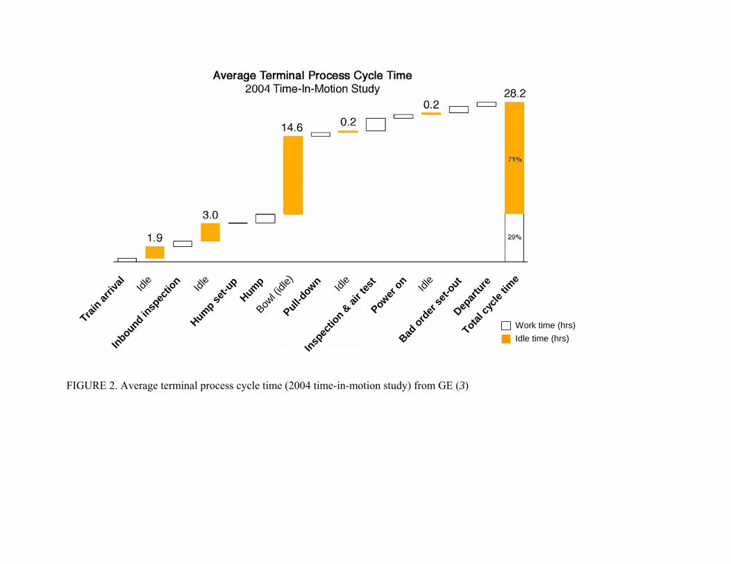
The bottleneck can be identified by analyzing where cars spend time as they flow through the

yard. A time-and-motion study conducted by the GE Yard Solutions group for one classification

yard found that cars were idle for 71% of the 28.2-hour average dwell time in the yard (Figure

2). The largest portion of this time (14.6 hours) was spent in the classification yard (or bowl). A

disproportionately long wait time immediately upstream from a production process is a good

indicator that process is the bottleneck. This indicates that the pull-down process is the

bottleneck. This is consistent with previously published work (5, 16, 17) and railroad

management experience at CPR, CN and UP (18).

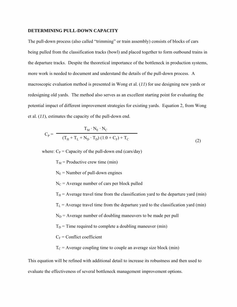
DETERMINING PULL-DOWN CAPACITY

The pull-down process (also called “trimming” or train assembly) consists of blocks of cars

being pulled from the classification tracks (bowl) and placed together to form outbound trains in

the departure tracks. Despite the theoretical importance of the bottleneck in production systems,

more work is needed to document and understand the details of the pull-down process. A

macroscopic evaluation method is presented in Wong et al. (11) for use designing new yards or

redesigning old yards. The method also serves as an excellent starting point for evaluating the

potential impact of different improvement strategies for existing yards. Equation 2, from Wong

et al. (11), estimates the capacity of the pull-down end.

(TH + TL + ND · TD) (1.0 + CF) + TCCP =

TM · NE · NC

(2)

where: CP = Capacity of the pull-down end (cars/day)

TM = Productive crew time (min)

NE = Number of pull-down engines

NC = Average number of cars per block pulled

TH = Average travel time from the classification yard to the departure yard (min)

TL = Average travel time from the departure yard to the classification yard (min)

ND = Average number of doubling maneuvers to be made per pull

TD = Time required to complete a doubling maneuver (min)

CF = Conflict coefficient

TC = Average coupling time to couple an average size block (min)

This equation will be refined with additional detail to increase its robustness and then used to

evaluate the effectiveness of several bottleneck management improvement options.

Operational Methods

The major activities performed by pull-down crews are coupling cars on the classification tracks

and then pulling them to the departure yard (11). Pull-down operational methods are closely

related to the design of the pull-down end of the yard and the orientation of the departure yard to

the classification yard. In parallel departure yard designs, the method of making up trains can

vary. The first method involves an engine pulling the cars on one track directly to the departure

yard and will be referred to as "single pull". In the second method, engines pull cars from

several tracks and then move them as a group to the departure yard, which will be referred to as

"multiple pull". In inline departure yard designs, trains are usually built with the multiple pull

method.

In practice, railroads tend to use the method most appropriate to the current operational

situation at the yard. The yardmaster decides what method or combination of the two (i.e. the

crew on engine 2026 builds Train 291 with multiple pull and the crews on engines 1543 and

4608 build Train 287 with single pulls) will be employed based on his or her preference,

experience of the pull-down crews, work load, track maintenance and potential interference on

the switch leads.

A detailed analysis of the pull-down process was conducted at Bensenville Yard (CPR)

near Chicago. Bensenville has a parallel departure yard design and both operational methods are

used. However, because single pull was the predominant method used, ND (the average number

of doubling maneuvers to be made per pull) can now be used to reflect a similar activity, rework.

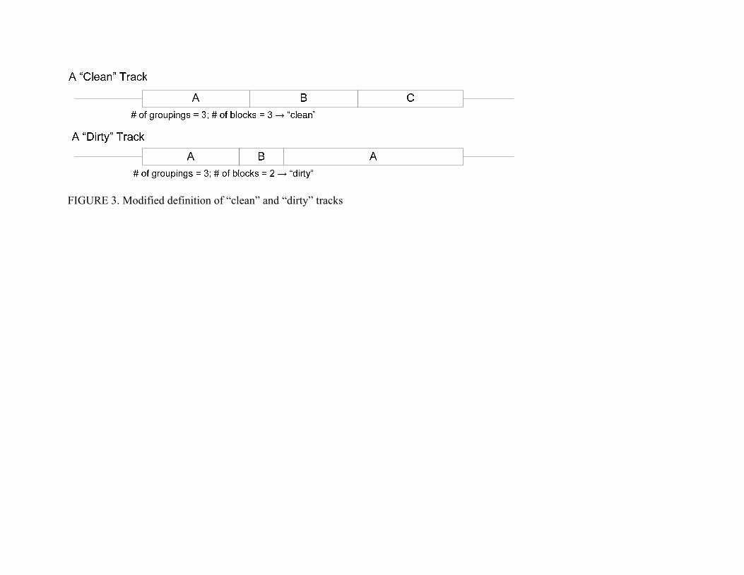
“Clean” and “Dirty” Tracks

Rework occurs on the pull-down end when tracks are “dirty.” A slight modification of Kraft's

(9) definition of “clean” and “dirty” tracks will be used to compare the number of groupings to

the number of blocks. A grouping is a group of cars in standing order all having the same block,

if there are more groupings than blocks, then at least one car must be out of place on that track

(Figure 3). The additional switching work that is required when a track is dirty is similar to the

work required when “cherry-picking” (5), which is the pulling of high-priority cars located

behind other cars on a bowl track.

Cycle Time Components

All of the time parameters in Equation 2 (TM, TH, TL, TD, TC) need to be determined by

conducting time studies. The first, the productive crew time (TM), is the time that the crew is

doing productive work. The maximum possible productive crew time is 1,440 minutes per day,

minus the total minutes for meals and breaks (11). However, this value should be further refined

to reflect real work conditions. No crew can maintain a maximum pace every minute of the

work day because of interruptions, fatigue and unavoidable delay (19). Also, crews will exert

different effort levels depending on a variety of factors such as skill level, motivation and age.

The result is a reduction in the productive crew time and can be accounted for with Equation 3.

TM = (1440 – MB) · PF (3)

where: TM = Productive crew time (min)

MB = Total meal and break time (min)

PF = Performance factor

The remaining time parameters can be added together to calculate the cycle time of the

pull-down process (Equation 4). The cycle time is the time it takes to complete one cycle of the

process.

CT = TL + TC + BR·TD + TH + DR·TD (4)

where: CT = Average pull-down process cycle time (min)

TL = Average travel time from the departure yard to the classification yard (min)

TC = Average coupling time to couple an average size block (min)

TD = Time required to complete a doubling maneuver (min)

TH = Average travel time from the classification yard to the departure yard (min)

BR = Bowl rework occurrence integer (0 or 1)

DR = Departure yard rework occurrence integer (0 or 1)

BR + DR < 1

For the pull-down process, the cycle time begins when the crew receives the switch list from the

yardmaster. It ends when the crew uncouples from the cut of cars after placing them on the

required track in the departure yard. The high-level process flow diagram in Figure 4 illustrates

this procedure and breaks it into five cycle time components: setup (TL), coupling (TC), bowl

rework (B·TD), transport (TH) and departure yard rework (D·TD). It is assumed for this model

that rework will only occur at most one time per pull; either in the bowl or in the departure yard.

BOTTLENECK MANAGEMENT IMPROVEMENT ALTERNATIVES

Pull-down time studies were conducted at Bensenville over a period of four days during March

2006. The time of day that the observations were gathered was different each day. A total of

fifteen complete cycles were observed during the available time period. The data from those

studies were used, along with other yard measurement data normally tracked by CPR, to

calculate the parameters for Equations 3 and 4 (Table 1). This allowed for Equation 2 to be used

to estimate the capacity of the pull-down process for a baseline case. Individual parameters, and

combinations of parameters, were then modified to determine the potential capacity increase for

each alternative (Table 2). The boxes in each column highlight the parameter or parameters that

were changed from the baseline.

The baseline case has an estimated capacity of 541 cars per day. To check the accuracy

of the estimate, the average daily process car count for 2004 was calculated. CPR defines

process cars as cars that go through all yard processes: arrival, classification, pull-down and

departure. The average throughput was 521 cars per day. Average throughput should be less

than theoretical capacity (1); therefore, the estimate is acceptable.

Option 1: Add another pull-down engine

One option to increase capacity at the pull-down end is to add another engine. This was the first

alternative tested and it resulted in a capacity of 576 cars per day, an increase of 6.5%. The

limiting factor when adding another engine is the increased conflict coefficient (2.55 vs. 1.55).

Other yard designs may have higher conflict coefficients that will further limit effectiveness.

While this option results in the one of the highest capacity levels, it is also the most expensive

because of the additional engine and labor cost.

Option 2: Pull from the hump end when idle

At Agincourt Yard (CPR) in Toronto, an option has been implemented that increases capacity

without increasing interference or engine and labor costs. The hump engine is used to build

trains when the hump is idle. This is done by placing the hump in trim mode (disabling the

retarders), allowing the engine to enter the bowl and pull blocks from the hump end. Agincourt,

like Bensenville, has parallel receiving and departure yards. This solution would not be practical

for yards with in-line designs.

This solution follows the TOC approach. Having identified the system’s constraint, yard

management was able to exploit the pull-down process by subordinating one of the other

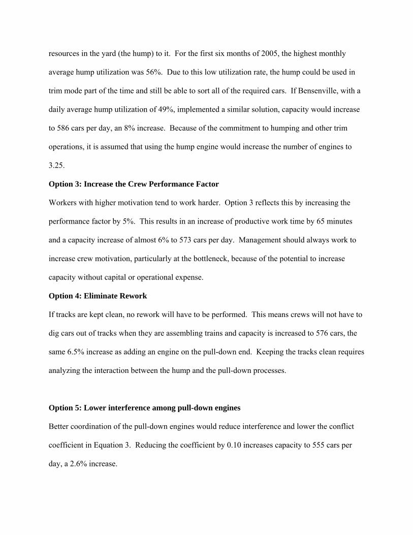
resources in the yard (the hump) to it. For the first six months of 2005, the highest monthly

average hump utilization was 56%. Due to this low utilization rate, the hump could be used in

trim mode part of the time and still be able to sort all of the required cars. If Bensenville, with a

daily average hump utilization of 49%, implemented a similar solution, capacity would increase

to 586 cars per day, an 8% increase. Because of the commitment to humping and other trim

operations, it is assumed that using the hump engine would increase the number of engines to

3.25.

Option 3: Increase the Crew Performance Factor

Workers with higher motivation tend to work harder. Option 3 reflects this by increasing the

performance factor by 5%. This results in an increase of productive work time by 65 minutes

and a capacity increase of almost 6% to 573 cars per day. Management should always work to

increase crew motivation, particularly at the bottleneck, because of the potential to increase

capacity without capital or operational expense.

Option 4: Eliminate Rework

If tracks are kept clean, no rework will have to be performed. This means crews will not have to

dig cars out of tracks when they are assembling trains and capacity is increased to 576 cars, the

same 6.5% increase as adding an engine on the pull-down end. Keeping the tracks clean requires

analyzing the interaction between the hump and the pull-down processes.

Option 5: Lower interference among pull-down engines

Better coordination of the pull-down engines would reduce interference and lower the conflict

coefficient in Equation 3. Reducing the coefficient by 0.10 increases capacity to 555 cars per

day, a 2.6% increase.

Option 6: Decrease component cycle times

Faster cycle times result in increased process throughput. Cycle times can be reduced by

eliminating unnecessary moves, throwing fewer switches, increasing engine speed, preventing

engine breakdown, using experienced crews, etc. For option 6, it was assumed that the average

travel times from the bowl to departure yard (TH) and departure yard to bowl (TL) as well as the

average time for rework (TD) were all reduced by 1 minute. This would increase capacity

approximately 4% to 564 cars.

Option 7: Decrease coupling time

Several factors affect the time it takes to couple the cars on the bowl track, including walking

speed, number of cars on the track, switch-list discrepancies and the number, spacing and

location of gaps between cars. In Bensenville, crews also have the option of walking back to the

engine or riding the last car out. It is up to the crew to decide the safest option. Coupling time

could be reduced by eliminating gaps through better retarder control or humping multiple-car

cuts when possible, more accurate track inventory control and equipment to help the crew correct

out-of-alignment drawbars more quickly. For Option 7, the safest alternative (walking out) was

maintained and average coupling time was decreased 5 minutes. The resultant capacity increase

was 21 cars per day, an improvement of just under 4%.

Combining Multiple Improvement Alternatives

Each option does not have to be implemented in isolation. The second to last column in Table 2

combines Options 2, 4, 5, 6, and 7. All of the options are process improvement initiatives and

require minimal investment. Capacity was increased 28% over the baseline case to 695 cars per

day. The last column adds the impact of increasing crew motivation (Option 3) to the previous

column. Capacity was increase by an additional 41 cars per day, 36% greater than the baseline

case.

REDUCING THE OCCURANCE OF REWORK

Because a classification yard is a system, managing the interactions between the processes is just

as important as managing the individual processes. All but two of the options above improve

only the pull-down process. Those involving the interaction between the pull-down and the

hump (Options 2 and 4) result in greater capacity increases. This is consistent with the Theory of

Constraints.

One of the principal findings of this work is that the humping process should be

subordinate to the pull-down process. Because the pull-down is the bottleneck, the hump should

be managed and operated so that it provides the bottleneck exactly what it needs when it needs it.

The practice of measuring hump performance merely on number of cars processed can and often

does contribute to poor pull-down performance because it can lead to incorrectly sorted cars. In

order to better manage the interaction between the hump and the pull-down processes, a

measurement of how well the cars are being sorted is needed. The Quality of Sort metric was

developed to provide a better measure of the impact that sorting has on the workload of the pull-

down process.

The Quality of Sort Metric

The metric is called the Incorrect Sort Rating (ISR) and is built in three levels: car, track and

bowl. The unit of measurement is number of cars and a low ISR indicates fewer incorrectly

sorted cars. At the car level, every car that is humped into the bowl is rated according to three

components. Each component is weighted according to the impact that it has on the pull-down

workload.

Car ISR = RT + RG + BI s.t. RT = 0 or α; RG = 0 or β;

BI = 0 or µ; α + β + µ = 1 (5)

The first component (RT) in Equation 5 is used to measure the adherence to a static track

allocation scheme if one is in place and is called Right Car-Right Track. The second component

(RG) recognizes the need for flexibility of the static track allocation scheme and is called Right

Car-Right Group. The third component (BI) is called Block Integrity and takes into account the

extra workload caused by a car having a different block than the previous car on that track.

An example from Alyth Yard (CPR) is used to illustrate Equation 5. Car ICE 70512 has

classification code 4850MA1 (St. Paul Manifest Block) and that block is assigned to track CT12

(Central Group) in the bowl. CT12 is the destination track. If the actual track that ICE 70512 is

humped to equals the destination track (CT12), then RT=0 and RG=0. If actual track does not

equal destination track, then RT=α and RG=0 if the actual track is in the Central Group;

otherwise, RG=β. BI=0 if the previous car on the actual track is from the same block (St. Paul

Manifest) as ICE 70512. BI=µ if the previous car on the actual track is from a different block.

The track level reflects the fact that the pull-down process works by track. The ISR

values for every car on a track are summed and a multiplier reduces the total if the track is clean

(δ), or increases the total if the track is dirty (η).

Track ISR = {∑all cars on track n Car ISR} x TF s.t. TF = δ or η (6)

The Track ISR value for designated mechanical and re-hump tracks is not multiplied by TF

because they are supposed to be dirty and subjecting them to the multiplier would artificially

inflate the ISR. Weighting the metric this way provides an incentive for humpmasters to keep

the tracks in the bowl clean.

The bowl level of the metric is the highest level and reflects the overall performance of

the hump controller in maintaining a “clean” bowl. The bowl ISR is the sum of the Track ISR

values for every track in the bowl except the designated mechanical tracks. The mechanical

tracks are ignored because they are subject to a different pulling process.

Bowl ISR = ∑for all non-mechanical tracks Track ISR (7)

Before the Bowl ISR can be used to gauge a hump controller’s performance and better

manage the interaction between the hump and the pull-down, the expected Bowl ISR over a

range of bowl volume levels needs to be known. In order to understand these relationships, a

Bowl Replay program was developed to analyze yard event data. The first operational version

was completed for Alyth Yard and a second version was developed for Bensenville. See

Dirnberger (10) for a detailed description of the program.

Bowl ISR vs. Bowl Volume

The weighted values were assigned to the ISR components based upon management feedback.

At the car level, breaking block integrity was unequivocally considered the greatest detriment to

pull-down throughput; therefore, µ was assigned a value of 0.50. The wrong track and wrong

group components were rated equally with α and β assigned values of 0.25. For the TF

component of the Track ISR level (Equation 6), clean track values are multiplied by δ=0.5 and

dirty tracks by η = G – B where: G = number of groupings and B = number of blocks. When

cars are pulled from the bowl, their ISR values are removed from the totals. The impact of trim

events is also reflected in the ISR subject to the three quality components but with an added

penalty for the extra work. The program continually records the bowl volume and bowl ISR for

use in the development of the relationship between those two parameters.

To develop the relationship presented here, a bowl replay for Alyth Yard using event data

for a five-day period was built. A total of 5,060 observations of bowl volume and corresponding

ISR were recorded. The observations were grouped by volume level and any volume level with

less than nine observations was discarded. Averages for the remaining observations were

calculated and plotted (Figure 5) and the expected trend of a higher volume resulting in a

“dirtier” bowl is seen.

Implementing the Metric

To be successfully used as part of a yard management system, the information must be presented

to the humpmaster and other yard management in an appropriate fashion and close to real-time.

A visual representation of the bowl, similar to the Bowl Integrity screen of CN’s Smart Yard™

system that uses colors to identify cars from different blocks on the same track, would provide a

quick assessment of the current number of dirty tracks. Adding the metric to this would enable

the use of Statistical Process Control (SPC) techniques such as X-Bar charts to track the ISR

level, provide performance feedback to humpmasters and identify root causes of an excessively

dirty bowl or track. In addition, a decision support system could be designed using the metric to

aid the humpmaster in determining the best location to place a car or block of cars based on the

current state of the bowl.

CONCLUSIONS

Production systems often focus too much on quantity and not enough on quality. Hump yards

are no exception. Hump controllers are rated primarily on the number of cars humped during

their shift with little emphasis placed on how well they have sorted those cars. The Quality of

Sort metric should be used in a yard management system to emphasize the importance of

preventing and correcting defects at the hump end of a yard. For Bensenville Yard, doing so

would result in an estimated 6.5% pull-down capacity increase; the same as adding another pull-

down engine. Other yards could expect to obtain similar results. Sustaining this quality

emphasis will require management focus to shift from the hump to the pull-down process.

The insights of factory physics and TOC indicate that focusing more attention on the

productivity of the pull-down process will result in increased yard capacity. Several bottleneck

management alternatives were presented and their impact on capacity evaluated. Of the

alternatives presented, the two improving the interaction between the hump and the pull-down

processes resulted in the greatest capacity increases. Pull-down capacity at Bensenville Yard can

be increased an estimated 36% by improving the process and its interactions without adding any

engine or labor expense. The lean emphasis on reducing idle time between all yard processes

will further increase capacity. By combining scheduled railroading with a version of Lean

Manufacturing in their yards, CPR reports average terminal dwell fell from 30.4 hours in March

2005 to 20.7 hours in March 2006 (20). Assuming a constant terminal volume of 1,500 cars, this

results in an estimated average terminal capacity increase of 555 cars per day (Equation 1), a

47% increase.

ACKNOWLEDGEMENTS

The first author was supported by a CN Railroad Engineering Research Fellowship. Both

authors are grateful for the assistance provided by the Canadian Pacific Railway, the CN

Railway and Prescott Logan of GE Yard Solutions during the course of this research. They

would also like to thank Darwin Schafer for his assistance gathering and analyzing data and

Justin Wood for his help with the VBA code for the program. Both are students at the University

of Illinois.

REFERENCES

1. Hopp, W.J. and M. L. Spearman. Factory Physics: Foundations of Manufacturing

Management, 2nd Ed., McGraw-Hill, Boston, MA, (2001).

2. Martland, C.D., Little, P., Kwan, O.K. and R. Dontula. Background on Railroad Reliability.

AAR Report No. R-803, Association of American Railroads, Washington, DC, (1992).

3. Logan, P. “People, Process, and Technology – Unlocking Latent Terminal Capacity”,

Transportation Research Board 85th Annual Meeting presentation, (2006).

4. Kwan, O.K., Martland, C.D., Sussman, J. M. and P. Little. “Origin-to-Destination Trip

Times and Reliability of Rail Freight Services in North American Railroads”,

Transportation Research Record, 1489, pp. 1-8, (1995).

5. Kraft, E. R. “Priority-Based Classification for Improving Connection Reliability in Railroad

Yards Part I of II: Integration with Car Scheduling”, Journal of the Transportation Research

Forum published in Transportation Quarterly, Vol. 56, No. 1, pp. 93-105, (2002).

6. Kraft, E. R. “Priority-Based Classification for Improving Connection Reliability in Railroad

Yards Part II of II: Dynamic Block to Track Assignment”, Journal of the Transportation

Research Forum published in Transportation Quarterly, Vol. 56, No. 1, pp. 107-119,

(2002).

7. Ytuarte, C. “Getting over the hump”, Railway Age, October 2001, pp. 29-30, (2001).

8. Kraft, E. R. “Implementation Strategies for Railroad Dynamic Freight Car Scheduling”,

Journal of the Transportation Research Forum, Vol. 39, No. 3, pp. 119-137 (2000).

9. Kraft, E. R. “A Hump Sequencing Algorithm for Real Time Management of Train

Connection Reliability”, Journal of the Transportation Research Forum, Vol. 39, No. 4, pp.

95-115 (2000).

10. Dirnberger, J.R. “Development and Application of Lean Railroading to Improve

Classification Terminal Performance”, Master’s Thesis, University of Illinois Urbana-

Champaign, (2006).

11. Wong, P.J., Sakasita, M., Stock, W.A., Elliott, C.V. and M.A. Hackworth. Railroad

Classification Yard Technology Manual – Volume I: Yard Design Methods. FRA/ORD-

81/20.I, Final Report. National Technical Information Service, Springfield, VA, (1981).

12. Dirnberger, J.R. and C.P.L. Barkan. “Implementing Bottleneck Management Techniques

and Establishing Quality of Sort Relationships to Improve Terminal Processing Capacity”,

Proceedings of the 7th World Congress on Railway Research, Montreal (June 2006).

13. Rother, M. and J. Shook. Learning to See: Value Stream Mapping to Create Value and

Eliminate Muda – Version 1.2. The Lean Enterprise Institute, Brookline, MA, (1999).

14. Spearman, M.L. ‘To Pull or Not To Pull, What is the Question? Part II: Making Lean Work

in Your Plant’, White Paper Series, Factory Physics, Inc., College Station, TX, (2002).

[Online] Available from: www.factoryphysics.net [August 20, 2004].

15. Goldratt, E.M. Theory of Constraints. North River Press, Great Barrington, MA, (1990).

16. Petersen, E. R. Railyard Modeling: Part I. Prediction of Put-Through Time. Transportation

Science, Vol. 11, No. 1, pp. 37-49, (1977).

17. Petersen, E. R. Railyard Modeling: Part II. The Effect of Yard Facilities on Congestion.

Transportation Science, Vol. 11, No. 1, pp. 50-59, (1977).

18. McClish, R. 2005 Analyst Meeting Presentation. Union Pacific Railroad, (2005). [Online]

Available from: http://www.up.com/investors/attachments/presentations/

2005/analysts_conf/mcclish.pdf [July 12, 2005].

19. Niebel, B.W. and A. Freivalds. Methods, Standards, and Work Design, 10th Ed.,

WCB/McGraw-Hill, Boston, MA, (1999).

20. Canadian Pacific Railway. Key Metrics [Online], Available from:

http://www8.cpr.ca/cms/English/Investors/Key+Metrics/default.htm. [May 31, 2006].

LIST OF TABLES

TABLE 1. Calculated parameters for baseline case, Bensenville Yard (CPR)

TABLE 2. Estimated capacity increases for various bottleneck improvement alternatives

LIST OF FIGURES

FIGURE 1. Distribution of freight car time on CPR, first nine months 2004

FIGURE 2. Average terminal process cycle time (2004 time-in-motion study) from GE (3)

FIGURE 3. Modified definition of “clean” and “dirty” tracks

FIGURE 4. Pull-down process cycle time components

FIGURE 5. Average ISR vs. bowl volume for Alyth Yard, September 13 to 17, 2005

Paramter Value NotesMB = Total meal and break time (min) 135 30 min lunch, 15 min other breaks, 3 shiftsPF = Performance factor 0.85 85% has been used as standard in yards (Logan unpublished date )TM = Productive crew time (min) 1109 TM = (1440 – MB) · PF

CT = Average pull-down process cycle time (min) (no rework) 79 Net travel time, no conflictsCT = Average pull-down process cycle time (min) (with rework) 98 Net travel time, no conflictsTL = Average travel time from the departure yard to the classification yard (min) 10 Net travel time, no conflictsTC = Average coupling time to couple an average size block (min) 48 Calculated using bowl authority logs, Dec. 26 to Jan. 2, for 22 carsTD = Time required to complete a doubling maneuver (min) = rework 19 Net travel time, no conflictsTH = Average travel time from the classification yard to the departure yard (min) 21 Net travel time, no conflictsNE = Number of pull-down engines (engines) 3 Three crews per shift on averageNC = Average number of cars in a cut of a block (cars) 22 Dec. 24, 2005 to Jan. 10, 2006 averageND = Average number of doubling maneuvers to be made per pull 0.17 Over 4 day period, average of 17% dirty tracks pulled per dayCF = Conflict coefficient 1.55 from Wong et al. (18 ) pg. 149, Configuration 1 with 3 engines

TABLE 1. Calculated parameters for baseline case, Bensenville Yard (CPR)

Parameter Baseline(1) Add Engine

at pull-down

(2) Use hump engine when

idle(3) Increase PF by 5% (4) No rework

(5) Lower interference

(6) Cycle times 1 min less

(7) Coupling time 5 min less

Combine 2,4,5,6,7

Combine 2,3,4,5,6,7

TM = 1109 1109 1109 1174 1109 1109 1109 1109 1109 1174NE = 3 4 3.25 3 3 3 3 3 3.25 3.25NC = 22 22 22 22 22 22 22 22 22 22TH = 21 21 21 21 21 21 20 21 20 20TL = 10 10 10 10 10 10 9 10 9 9ND = 0.17 0.17 0.17 0.17 0 0.17 0.17 0.17 0 0TD = 19 19 19 19 19 19 18 19 18 18CF = 1.55 2.55 1.55 1.55 1.55 1.45 1.55 1.55 1.45 1.45TC = 48 48 48 48 48 48 48 43 43 43CP = 541 576 586 573 576 555 564 562 695 736

TABLE 2. Estimated capacity increases for various bottleneck improvement alternatives

9% 10%

30%

9% 8%

34%

0%

5%

10%

15%

20%

25%

30%

35%

40%

Shpper dwell Loadedtransit

Loaded yarddwell

Consigneedwell

Emptytransit

Empty yarddwell

Activity

Perc

enta

ge o

f tot

al ti

me

FIGURE 1. Distribution of freight car time on CPR, first nine months 2004 (CPR unpublished date)

Train a

rriva

l

Idle

Inboun

d ins

pectio

n Idle

Bowl (i

dle)

Hump se

t-up

Hump

Pull-dow

n Idle

Idle

Power

onBad

order

set-o

utTotal

cycle

time

Depart

ure

Inspe

ction &

air t

est

Work time (hrs)Idle time (hrs)

FIGURE 2. Average terminal process cycle time (2004 time-in-motion study) from GE (3)

FIGURE 3. Modified definition of “clean” and “dirty” tracks

FIGURE 4. Pull-down process cycle time components

0

20

40

60

80

100

120

350 400 450 500 550 600 650BV = Bowl volume (number of cars)

Ave

rage

ISR

(num

ber o

f car

s)

FIGURE 5. Average ISR vs. bowl volume for Alyth Yard, September 13 to 17, 2005