Improving Software Pipelining with Unroll-and-Jam and Memory Reuse Analysis By Chen Ding A THESIS Submitted in partial fulfillment of the requirements for the degree of MASTER OF SCIENCE IN COMPUTER SCIENCE MICHIGAN TECHNOLOGICAL UNIVERSITY 1996
Transcript
Improving Software Pipelining
withUnroll-and-Jam and Memory Reuse Analysis
By
Chen Ding
A THESIS
Submitted in partial fulfillment of the requirements
for the degree of
MASTER OF SCIENCE IN COMPUTER SCIENCE
MICHIGAN TECHNOLOGICAL UNIVERSITY
1996
ii
This thesis, “Improving Software Pipelining with Unroll-and-Jam and Memory Reuse
Analysis”, is hereby approved in partial fulfillment of the requirements for the Degree of MASTER
OF SCIENCE IN COMPUTER SCIENCE.
DEPARTMENT of Computer Science
Thesis Advisor Dr. Philip Sweany
Head of Department Dr. Austin Melton
Date
iii
AbstractThe high performance of today’s microprocessors is achieved mainly by fast, multiple-
issuing hardware and optimizing compilers that together exploit the instruction-level parallelism
(ILP) in programs. Software pipelining is a popular loop optimization technique in today’s ILP
compilers. However, four difficulties may prevent the optimal performance of software pipelining:
insufficient parallelism in innermost loops, the memory bottleneck, hardware under-utilization due
to uncertain memory latencies, and unnecessary recurrences due to the reuse of registers (false
recurrences).
This research uses an outer-loop unrolling technique, unroll-and-jam, to solve the first and
second problems. It shows, both in theory and experiment, that unroll-and-jam can solve the first
problem by exploiting cross-loop parallelism in nested loops. Unroll-and-jam can also automatically
remove memory bottlenecks for loops. This research discovered that for 22 benchmark and kernel
loops tested, a speed improvement of over 50% is obtained by unroll-and-jam.
For solving the uncertain memory latencies, this research uses a compiler technique,
memory reuse analysis. Using memory reuse analysis can significantly improve hardware uti-
lization. For the experimental suite of 140 benchmark loops tested, using memory reuse analysis
reduced register cycle time usage by 29% to 54% compared to compiling the same loops assuming
all memory accesses were cache misses.
False recurrences restrict the use of all available parallelism in loops. To date, the only
method proposed to remove the effect of false recurrences requires additional hardware support
for rotating register files. Compiler techniques such as modulo variable expansion [25] are neither
complete nor efficient for this purpose. This thesis proposes a new method that can eliminate the
effect of false recurrence completely at a minimum register cost for conventional machines that do
not contain rotating register files.
iv
Acknowledgments
I would like to thank my primary advisor, Dr. Phil Sweany, for giving me this interesting
work and supporting me, both technically and emotionally, throughout my two-year study. Without
him, this thesis would not be possible. I would like to thank Dr. Steve Carr for his tremendous help,
encouragement and support. The close working relationship with them has taught me true sense
of research and character of a computer scientist. Sincere thanks also go to my other committee
members, Dr. David Poplawski and Dr. Cynthia Selfe, for their feedback and encouragement,
to all other faculties in the Computer Science department, whose knowledge and support have
greatly strengthened my preparation for a career in computer science, and to all my fellow graduate
students, whose constant caring and encouragement have made my life more colorful and pleasant.
Being a foreign student, English would have been a formidable obstacle without the help
from numerous friendly people. Dr. Phil Sweany and his wife, Peggie, have given me key help in
the writing of my proposal and this thesis. My writing skill has been significantly improved by a
seminar taught by Dr. Phil Sweany, Dr. Steve Carr and Dr. Jeff Coleman, and a course taught by
Dr. Marc Deneire. Dr. Marc Deneire also provided me direct professional guidance on the writing
of this thesis. I also want to acknowledge the valuable help, both on my written and spoken English
skills, from various student coaches in the Writing Center of the Humanity department.
Special thanks go to my wife, Linlin, whose love has always been keeping me warm and
happy. Last, I want to thank my parents. Without their foresight and never-ending support, I could
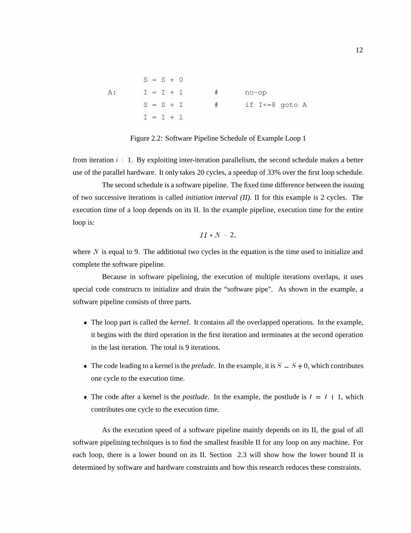
where k is one less than the integer part of n divided by 3. The new II will be 3 times the original II.
An obvious concern here is what to do with the rest of iterations when loop count n is
not a multiple of 3. One solution is loop conditioning, which adds an appropriate number of non-
pipelined iterations before the prelude (preconditioning), or after the postlude (postconditioning) to
ensure that the new kernel will be executed k times where k is a multiple of the unroll factor. If n
in the above example is 20, a non-pipelined schedule of loop that has a loop count 2 needs to be
added either before the prelude or after the postlude of the software pipeline.
32
When there are multiple lifetimes that are greater than II and each lifetime requires a
different degree of unrolling, the degree of kernel-unrolling can be determined by two different
methods[25]. One needs a larger number of unrolling (code expansion) but requires fewer registers;
the other requires more registers but less unrolling.
After kernel unrolling, the code generation step generates prelude, kernel and postlude.
Pre-conditioning or post-conditioning is needed for DO-loops if the kernel is unrolled. For WHILE-
loops, special techniques have been developed by Rau et al[35].
If a loop has undergone if-conversion and the machine does not have hardware support
for predicate execution, the branch constructs must be recovered in the code generation step. Warter
et al. describes this technique in [44].
2.4.4 Register Allocation
Current popular register assignment methods in ILP compilers are based on a graph
coloring formulation in which each scalar is a graph node, and each edge indicates that the lifetimes
of two values connected by the edge overlap with each other. So the register assignment problem
becomes a node-coloring problem where we want to use the fewest number of colors (registers) to
color all nodes such that no adjacent nodes share a color.
To minimize the register usage of software pipelines, a scheduling method should choose
a schedule that attempts to conserve registers. However, it is difficult for scheduling methods to
estimate register usage or to predict the result of register assignment because until after scheduling,
complete information about register lifetimes is unavailable. This section introduces three heuristic-
based register-assignment approaches for software pipelining. For optimal methods, readers are
referred to [17] [21].
Register Assignment after Register-Need-Insensitive Scheduling
Rau et al. investigated the register assignment problem of software pipelining[34]. They
studied various post-schedule register assignment methods. But they did not try to reduce the
register need in the scheduling step.
They tried different heuristics on both ordering lifetimes and assigning lifetimes to avail-
able registers. The three lifetime-ordering heuristics they tested are: ordering by starting time,
ordering by the smallest time difference with the previously scheduled one, and ordering by the
number of conflicts with other lifetimes. To map a lifetime to a register, there are also three
heuristics, best fit, first fit, and last fit.
33
For traditional machines that do not have rotating registers, the best heuristic, which
generates the best code and uses the least compile time, is ordering lifetimes by the number of
conflicts and mapping lifetimes to registers by first fit. In Rau et al.’s experiment, the best heuristic
used the same number of registers as MaxLive for 40% loops; and on average, it required 1.3 more
registers than MaxLive.
This work presented two notable results. First, the best heuristic is similar to graph-
coloring. So a general graph-coloring register assignment algorithm would probably do as well
as their best heuristic. Second, the measurement used for the lower bound on register demand,
MaxLive, is not necessarily the lower bound for the loop. MaxLive is dependent on a particular
schedule. It is possible that another schedule could have a lower MaxLive. Because the scheduler
used in Rau et al.’s research was not sensitive to register demand, it did not try to find that schedule
with the lowest MaxLive.
Register Assignment after Lifetime-Sensitive Scheduling
Huff [22] proposed a schedule-independent lower bound for register requirement. He
also modified iterative modulo scheduling so that the scheduling step attempts to minimize the
lifetime of values. The schedule-independent lower bound, MinAvg, has been described in Section
2.3.4. When an operation is scheduled in Huff’s scheduling method, a set of possible time slots
are identified. The heuristic favors a placement as early as possible in order to avoid lengthening
lifetimes involved in this operation.
Huff’s experimental results showed that 46% of loops achieved a MaxLive equal to
MinAvg and 93% of loops had a MaxLive within 10 registers of MinAvg. In his experiment,
hardware support of rotating registers is assumed [22]. For conventional hardware, the register
need is probably higher due to the effect of kernel unrolling.
Stage Scheduling to Minimize Register Requirement
Recently, a set of heuristics were developed by Eichenberger and Davidson [16] to find a
near optimal register assignment. Their method, called stage scheduling, is a post-pass scheduler
invoked after a software pipeline schedule has been found. They define a stage to be II cycles. In
stage scheduling, operations can only be moved in an integral number of stages ( thus a multiple
of II cycles). For any given software pipeline schedule, there is an optimal stage schedule that
requires the fewest registers among all possible schedules. Eichenberger and Davidson showed that
34
their heuristics achieves a performance only 1% worse than the optimal stage schedules. However,
optimal stage scheduling is not necessarily the optimal schedule with the lowest register needs since
stage schedules of a software pipeline do not include all possible software pipelines for a given II.
35
Chapter 3
Improving Software Pipelining with
Unroll-and-Jam
Unroll-and-jam is a loop transformation technique that unrolls outer loops and jams the
iterations of outer loops into the innermost loop. This chapter shows that unroll-and-jam has two
benefits to software pipelining. First, unroll-and-jam can exploit cross-loop parallelism for software
pipelining. Second, unroll-and-jam can automatically remove memory bottlenecks in loops. Section
1 describes the transformation of unroll-and-jam. Section 2 examines how unroll-and-jam can
exploit cross-loop parallelism for software pipelining. It shows that unroll-and-jam may create
new recurrences but the effect of these new recurrences can be eliminated by appropriate renaming
techniques. Thus, unroll-and-jam can exploit cross-loop parallelism for software pipelining without
restrictions. Section 3 examines the other benefit of unroll-and-jam to software pipelining. Unroll-
and-jam has been shown to be very effective in automatically removing memory bottlenecks [7] [9].
Section 3 shows that the removing of memory bottlenecks can significantly decrease the resource
constraint of software pipelining and thus improve software pipelining’s performance. One difficulty
of using unroll-and-jam with software pipelining is that the prediction of register pressure of the
transformed loop is difficult. Previous register prediction schemes do not consider the effect of the
overlapping execution in software pipelining [9]. Section 4 discusses several possible approaches
that can help predict register pressure in software pipelining after unroll-and-jam. The final section
compares the effect of unroll-and-jam on software pipelining with some other loop transformation
techniques.
36
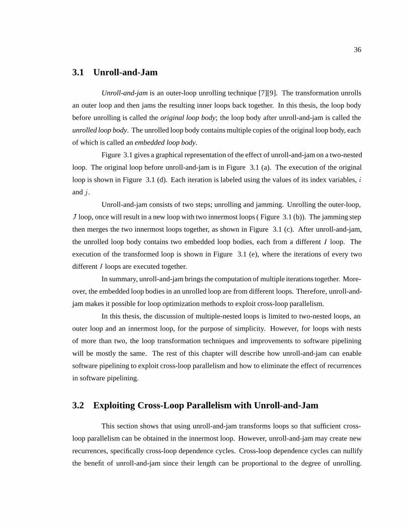
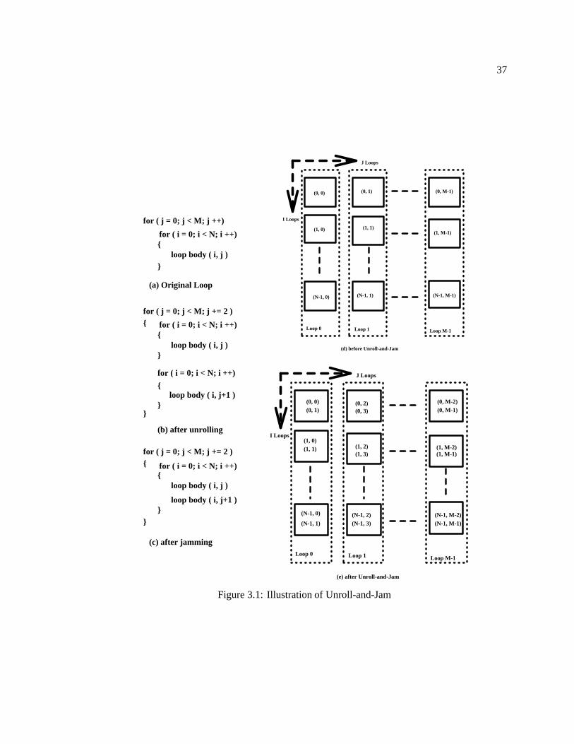
3.1 Unroll-and-Jam
Unroll-and-jam is an outer-loop unrolling technique [7][9]. The transformation unrolls
an outer loop and then jams the resulting inner loops back together. In this thesis, the loop body
before unrolling is called the original loop body; the loop body after unroll-and-jam is called the
unrolled loop body. The unrolled loop body contains multiple copies of the original loop body, each
of which is called an embedded loop body.
Figure 3.1 gives a graphical representation of the effect of unroll-and-jam on a two-nested
loop. The original loop before unroll-and-jam is in Figure 3.1 (a). The execution of the original
loop is shown in Figure 3.1 (d). Each iteration is labeled using the values of its index variables, i
and j.
Unroll-and-jam consists of two steps; unrolling and jamming. Unrolling the outer-loop,
J loop, once will result in a new loop with two innermost loops ( Figure 3.1 (b)). The jamming step
then merges the two innermost loops together, as shown in Figure 3.1 (c). After unroll-and-jam,
the unrolled loop body contains two embedded loop bodies, each from a different I loop. The
execution of the transformed loop is shown in Figure 3.1 (e), where the iterations of every two
different I loops are executed together.
In summary, unroll-and-jam brings the computation of multiple iterations together. More-
over, the embedded loop bodies in an unrolled loop are from different loops. Therefore, unroll-and-
jam makes it possible for loop optimization methods to exploit cross-loop parallelism.
In this thesis, the discussion of multiple-nested loops is limited to two-nested loops, an
outer loop and an innermost loop, for the purpose of simplicity. However, for loops with nests
of more than two, the loop transformation techniques and improvements to software pipelining
will be mostly the same. The rest of this chapter will describe how unroll-and-jam can enable
software pipelining to exploit cross-loop parallelism and how to eliminate the effect of recurrences
in software pipelining.
3.2 Exploiting Cross-Loop Parallelism with Unroll-and-Jam
This section shows that using unroll-and-jam transforms loops so that sufficient cross-
loop parallelism can be obtained in the innermost loop. However, unroll-and-jam may create new
recurrences, specifically cross-loop dependence cycles. Cross-loop dependence cycles can nullify
the benefit of unroll-and-jam since their length can be proportional to the degree of unrolling.
37
(0, 0) (0, 1) (0, M-1)
(1, 0) (1, 1)(1, M-1)
(N-1, 0) (N-1, 1)
Loop 0 Loop 1
(N-1, M-1)
Loop M-1
J Loops
(d) before Unroll-and-Jam
I Loops
Loop 0 Loop 1 Loop M-1
J Loops
I Loops
(0, 0)(0, 1)
(1, 0)(1, 1)
(N-1, 0)
(N-1, 1)
(0, 2)(0, 3)
(1, 2)(1, 3)
(N-1, 2)(N-1, 3)
(1, M-1)(1, M-2)
(0, M-1)(0, M-2)
(N-1, M-1)(N-1, M-2)
(e) after Unroll-and-Jam
for ( i = 0; i < N; i ++){
loop body ( i, j )
}loop body ( i, j+1 )
for ( j = 0; j < M; j += 2 ){
}
(c) after jamming
for ( i = 0; i < N; i ++){
loop body ( i, j )}
(a) Original Loop
for ( j = 0; j < M; j ++)
for ( j = 0; j < M; j += 2 ){ for ( i = 0; i < N; i ++)
{loop body ( i, j )
}
for ( i = 0; i < N; i ++)
{loop body ( i, j+1 )
}}
(b) after unrolling
Figure 3.1: Illustration of Unroll-and-Jam
38
This section categorizes cross-loop dependence cycles and describes how to eliminate the effect of
such cross-loop dependence cycles. As a result, unroll-and-jam can exploit cross-loop parallelism
without difficulties and eliminate the possible negative effect on the recurrence constraint of software
pipelining.
3.2.1 Cross-Loop Parallelism
Cross-loop parallelism is the parallelism existing among iterations of different loops in a
multiple-nested loop. Unroll-and-jam increases the amount of parallelism in the innermost loop by
exploiting cross-loop parallelism. As the amount of parallelism is measured by loop recurrences,
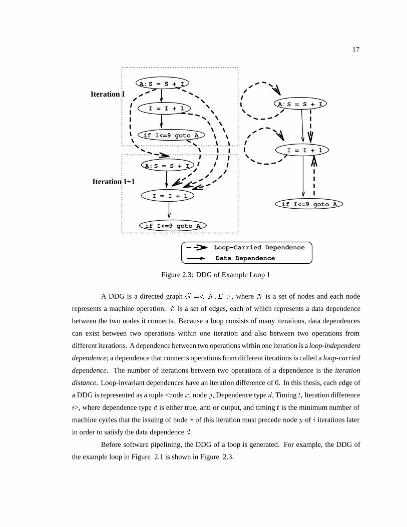
the effect of unroll-and-jam can be examined by comparing the data dependence graph (DDG) 1 of
the original loop body with the DDG of the unrolled loop body. Figure 3.2 shows how the DDG of
the unrolled loop body is changed after unroll-and-jam.
The DDG nodes in the unrolled loop body are copies of the DDG nodes of the original
loop body. The DDG nodes in the original loop body can be divided into two parts, control nodes
and computing nodes. Control nodes consist of the increment of the index variable, and the test on
the index variable deciding if the loop is finished. These nodes are part of the control structure of
the loop. Computing nodes are the remaining DDG nodes; those perform the computation during
each iteration. After unroll-and-jam, the computing nodes of the original loop body are duplicated
in each embedded loop body; however, only a single copy of the control nodes is required for the
entire unrolled loop body. For example, if a loop is unrolled N times, there will be N + 1 copies
of the computing nodes and 1 copy of control nodes in the DDG of the unrolled loop body. We call
each copy of the computing nodes in the unrolled loop body an embedded DDG and call the control
nodes the control DDG.
Figure 3.2 (c) and (d) show the DDGs of the original loop body and the unrolled loop
body of the example loop. Because the loop is unrolled once, there are two embedded loop bodies
in the unrolled loop body. The computing node of the original loop body is the assignment of a[i][j]
and the control node is the increment of i. The DDG of the unrolled loop body contains two copies
of the computing node (two embedded DDGs) and one copy of the control node (one control DDG).
The data dependences in the original loop body are also copied to the DDG of the unrolled
loop body. In the original loop body, a dependence is either (1) between two computing nodes, (2)
between a computing node and a control node, or (3) between two control nodes. Loop-invariant
1See Section 2.3.1 for a definition of DDG
39
(c) Recurrences in the innermost loop, before transforming
(d) Recurrences in the innermost loop, after transforming
for ( j = 0; j < M; j ++)
for ( j = 0; j < M; j += 2 )
for ( i = 0; i < N; i ++){
}
for ( i = 0; i < N; i ++)
{
(b) Loop after transforming
}
a[j] += b[i][j]
a[j] += b[i][j]
a[j+1] += b[i][j+1]
x a[j] += b[i][j]
i ++y
x
yy i ++
a[j+1] += b[i][j+1]x’a[j] += b[i][j]x
(a) Loop before transforming
Figure 3.2: Example Loop 2
40
dependences in the original loop body are copied exactly in the unrolled loop body: each dependence
between two computing nodes in the original loop body is duplicated in each embedded DDG; each
dependence between a computing node and a control node is duplicated between the computing node
in each embedded DDG and the control node in the control DDG; and each dependence between two
control nodes is copied in the control DDG. However, unroll-and-jam may add new dependences to
the unrolled loop body. These additional dependences are cross-loop dependences. The next section
shows how cross-loop dependences affect the DDG. However, loop-carried dependences that are not
cross-loop dependences are copied to the unrolled loop body in the same way as loop-independent
dependences. The example loop in Figure 3.2 does not have any cross-loop dependences; so all
data dependences, loop-independent and loop-carried, are simply duplicated in the DDG of the
unrolled loop body.
The important characteristic of the example DDG after unroll-and-jam is that no direct
data dependence exists between any two computing nodes of different embedded DDGs. This
determines that any loop-carried dependence cycle in the transformed loop is a copy of some loop-
carried dependence cycle in the original loop. So the length of the longest loop-carried dependence
cycle in the unrolled loop is the same as that in the original loop. This means that the recurrence
remains the same after unroll-and-jam. As the amount of computing is increased, the amount of
parallelism is increased. When unrolling N times, the amount of parallelism in the innermost loop
will be increased N + 1 times.
However, as previously mentioned unroll-and-jam may create new recurrences due to the
existence of cross-loop dependences. The new recurrences may restrict the available cross-loop
parallelism. The next two sections show that although unroll-and-jam may cause new recurrences,
the negative effect of the new recurrences on software pipelining can be eliminated.
3.2.2 Cross-Loop Dependences
A loop-carried dependence can exist between computing nodes of different iterations of the
same loop. Loop-carried dependence can also exist between computing nodes of different iterations
of different loops. The latter type of loop-carried dependence is called cross-loop dependence. For
example, in Figure 3.1 (e), if a dependence exists between an iteration inLoop 0 and an iteration in
Loop 1, it is a cross-loop dependence. Any dependence carried by the J loop must be a cross-loop
dependence. In fact, cross-loop dependences are dependences carried by outer loops.
41
(c) Recurrences in the innermost loop, before transforming
(d) Recurrences in the innermost loop, after transforming
for ( j = 0; j < M; j ++)
for ( j = 0; j < M; j += 2 )
for ( i = 0; i < N; i ++){
}
for ( i = 0; i < N; i ++)
{
(b) Loop after transforming
}
x
i ++y
x
yy i ++
x’x
s += b[i][j]
s += b[i][j]
s += b[i][j+1]
s += b[i][j]
s += b[i][j] s += b[i][j+1]
(a) Loop before transforming
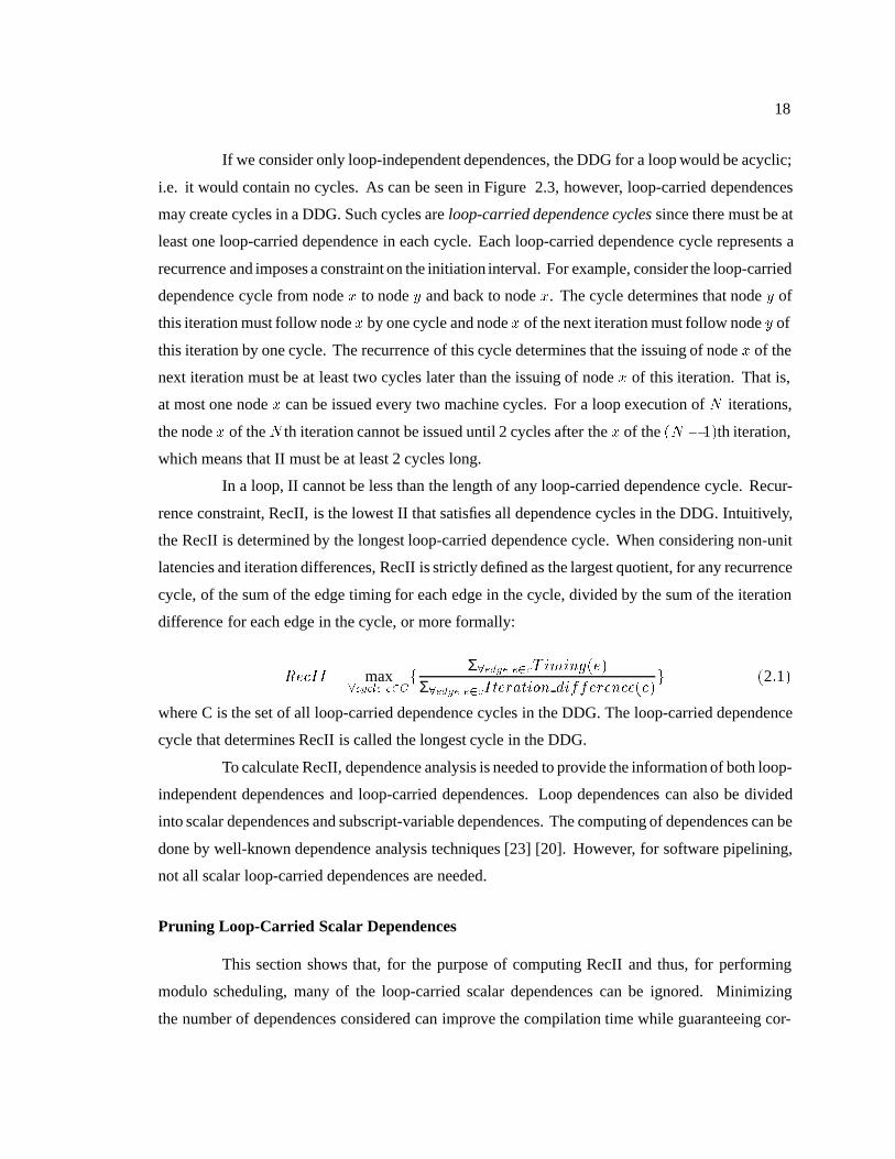
Figure 3.3: Example Loop 3
Because unroll-and-jam brings iterations of different loops together, cross-loop depen-
dences may be brought into the innermost loop and form new loop-carried dependence cycles in
the unrolled DDG. A loop-carried dependence cycle that has a cross-loop dependence edge is a
cross-loop dependence cycle.
For the example loop in Figure 3.2, there is no cross-loop dependence in the original
loop, so no dependence links the two embedded DDGs in the unrolled loop. However, for the
other example loop of Figure 3.3, there is a cross-loop dependence between iterations of unrolled
I loops. The cross-loop dependence is brought into the innermost loop by unroll-and-jam of the
original loop. It becomes two dependences: the loop-independent and the loop-carried dependences
between node x and x0. (Actually, each of the two dependences is three dependences, true, anti and
output. For simplicity, we assume they are one dependence.)
The cross-loop dependence causes two cross-loop dependence cycles in Figure 3.3 (d).
The first cross-loop dependence cycle includes node x and node x0. Both edges in this cycle are
42
cross-loop dependences. The second cross-loop dependence cycle links node x, x0 and y. The
cross-loop dependence from node x to node x0 links with the loop-independent dependence from
node x0 to y and the loop-carried dependence from node y to x. Though the latter two dependences
are just copies of existing dependences in the original loop body, they form a new recurrence when
linked with the cross-loop dependence.
Cross-loop dependence cycles are the new recurrences added by unroll-and-jam. In this
thesis, cross-loop dependence cycles are divided into two types, true cycles and false cycles. In a
true dependence cycle, all data dependences are true dependence edges; in a false cycle, at least one
dependence is a “false" dependence — that is at least one is either an anti-dependence or an output
dependence. The first new recurrence cycle in Figure 3.3(d) is a true cycle because all edges in
the cycle are true dependences. The next section will show that true cycles are caused by scalar
variables shared by both the innermost and the outer loop. In the example in Figure 3.3, the true
cycle is caused by variable S, which is shared by the I and J loops. The second new recurrence
cycle in Figure 3.3(d) is a false cycle since the loop-carried dependence, from node x0 to y, is an
anti dependence. False cycles are caused by the reuse of some scalar variable in the innermost loop.
In the example in Figure 3.3, the false cycle is caused by the reuse of the index variable i.
False cycles are of little interest since they are not inherent recurrences. False cycles
are a subset of false recurrences discussed in Chapter 5, and as such, can be eliminated in modulo
scheduling either by hardware support of rotating registers or by the renaming technique described
in Chapter 5. From now on, cross-loop dependence cycles only refers to true cycles in the loop
after unroll-and-jam.
True cross-loop cycles can nullify the benefit of cross-loop parallelism obtained by unroll-
and-jam. Unlike other dependence cycles that only include nodes of a single embedded DDG, such
true cross-loop cycles include nodes from all embedded DDGs. The length of the cross-loop
dependence is proportional to the degree of loop unrolling. New recurrences introduced by true
cycles limit the amount of parallelism in the innermost loop and makes more unrolling useless.
The following discussion of cross-loop dependence cycles focuses on the ‘global’ true
cycles that include the computing nodes of all embedded DDGs for any degree of unrolling. These
true cycles are the recurrences that can nullify the benefit of cross-loop parallelism obtained by
unroll-and-jam. A ‘global’ cross-loop dependence cycle (1) links every embedded DDG, and, (2)
links the same group of computing nodes within each embedded DDG.
43
3.2.3 Cross-Loop Dependence Cycles
True cycles must be caused by variables shared by both the innermost and the outer loop.
Consider Figure 3.1 (d). The iterations of the outer loop are called J loops and the iterations of the
inner loop are called I loops. A true cycle starts from each iteration in an I loop, goes through the
unrolled iterations in the corresponding J loop, and ends at the next iteration of the same I loop.
The data dependences of the true cycle mean that there is a scalar variable used and defined in both
the I and J loop. In other words, this scalar variable is shared in all loop iterations.
True cycles, which are caused by a shared variable, can be eliminated by shared-variable
renaming. To remove these cross-loop dependences, the shared variable should be renamed in each
embedded loop body. After using a different variable in each embedded loop body, the cross-loop
dependences are removed, and so is the cross-loop dependence cycle. Shared-variable renaming is
a special case of a well known technique, called tree height reduction[23]. Tree height reduction
divides the computation of the shared variable in the loop and completes the computation in a
minimum number of steps. The shared-variable renaming used in unroll-and-jam is equivalent to
dividing the overall computation into a number of parts equal to the unroll degree, which reduces
the recurrence length to 1n , where n is the degree of unrolling.
Figure 3.4 shows how shared variable renaming can eliminate the true cycle in Figure
3.3 (d). The true cycle in Figure 3.3 (d) is caused by variable S, which is shared in both I and J
loops. Assume iteration (i; j) and (i; j + 1) are executed together in the unrolled loop body. The
loop-carried data dependence from node x0 to x means that the computing of S in iteration (i; j+1)
must precede the computing of S in iteration (i+ 1; j). This is not a recurrence in the original loop,
since iteration (i+ 1; j) (in loop j) precedes iteration (i; j + 1) (in loop j+1) in the original loop.
The dependence is caused by the reuse of variable S. The order of computing S in two iterations
does not affect the semantics of the loop. That is, the computation of S in each iteration can proceed
in parallel if they do not reuse the variable S. So the true cycle can be removed if variable S is
renamed into two variables, S0 and S1 as in Figure 3.4 (b).
After renaming the shared variable S in the example loop in Figure 3.3, the renamed loop
and its new DDG are shown in Figure 3.4 (a) and (b). Now the DDG of the renamed loop body
contains no cross-loop dependence. By renaming the variable S, all cross-loop dependences of the
true cycle are removed.
If an outer loop is unrolled N times and a variable x is defined in each iteration, then
variable x should be renamed into x0, x2, ..., and xN�1 to eliminate the cross-loop dependence. In
44
for ( i = 0; i < N; i ++)
{
}yy i ++
x’x
for ( j = 0; j < M; j += 2 )
{
(b) Recurrences in the innermost loop, after renaming(a) Loop after renaming
s0 += b[i][j]
s1 += b[i][j+1]
s0 += b[i][j] s1 += b[i][j+1]
s += s0 + s1
}
Figure 3.4: Example of Shared-Variable Renaming
the unrolled loop body, each embedded loop body uses a different renamed variable. By eliminating
the cross-loop dependences among the embedded loop bodies in the unrolled loop, true cycles can
be removed.
3.2.4 Reducing Recurrence Constraints
Unroll-and-jam can increase the amount of parallelism in the innermost loop by exploiting
the cross-loop parallelism in the multiple-nested loop. By unrolling the outer loop N times, the
parallelism in the innermost loop can be increased to N times higher than before. To measure
the decrease on software pipelining constraints, we define the unit initiation interval (unit II) as II
divided by the unroll factor. Unit RecII is RecII divided by the unroll factor and Unit ResII is the
ResII divided by the unroll factor.
After removing cross-loop dependence cycles, the RecII is the same regardless of the
degree of the unrolling. But the unit RecII is decreased with respect to the degree of unrolling.
When the innermost loop is unrolledN times, the unit RecII of the unrolled loop body is 1N+1 of the
RecII in the original loop. Therefore, unroll-and-jam can always obviate the recurrence constraint
for nested loops by reducing the unit RecII until it is less than the unit ResII. This then guarantees
that the minimum II will be determined by the unit ResII rather than the unit RecII.
3.3 Removing the Memory Bottleneck with Unroll-and-Jam
Memory bottlenecks in software pipelining are caused by the limited number of memory
functional units and the high memory resource demand in loops. Unroll-and-jam, by unrolling
45
an outer loop and jamming iterations of different loops together, can effectively remove memory
bottlenecks and reduce the memory resource demand of the loop. This section describes how
unroll-and-jam removes memory operations and how software pipelining resource constraints can
be reduced by unroll-and-jam.
3.3.1 Removing Memory Operations
Scalar replacement, or load-store-elimination, has been used to reduce the number of
memory load/store operations by reusing values across innermost loop iterations[7] [5] [15] [10].
That is, instead of storing a value at this iteration and loading it at the next iteration, the value can
be maintained in a register and the load and store operations of that value can be eliminated.
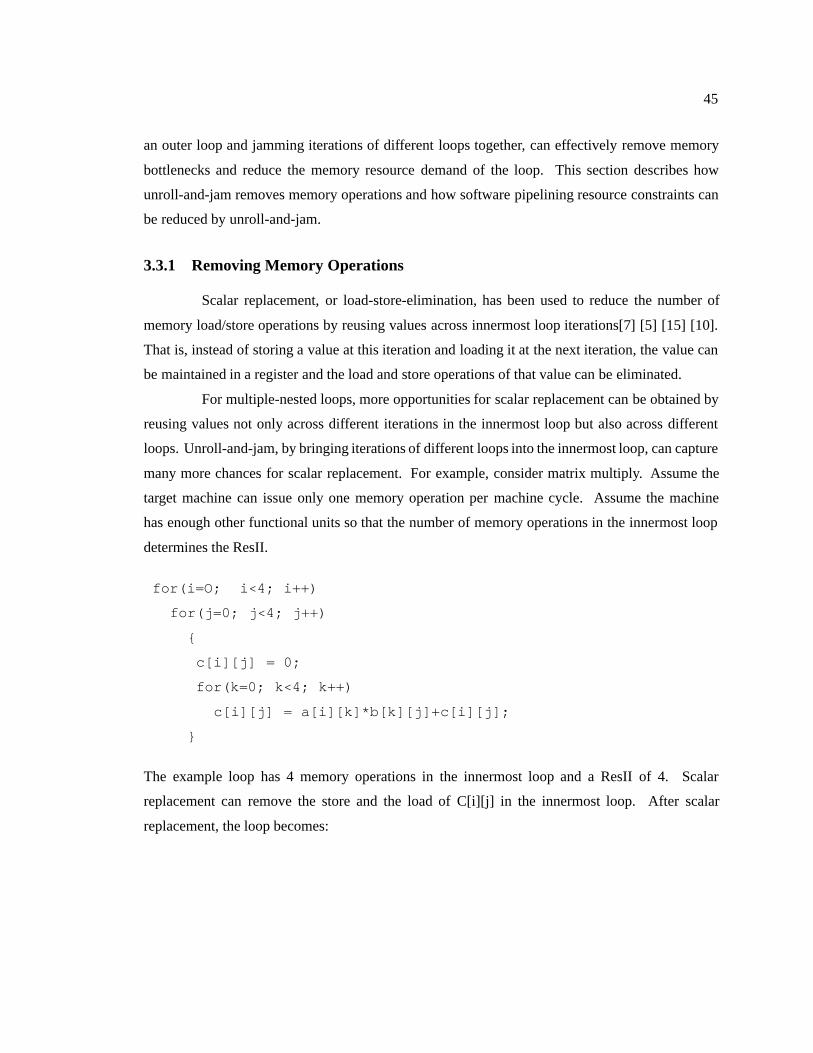
For multiple-nested loops, more opportunities for scalar replacement can be obtained by
reusing values not only across different iterations in the innermost loop but also across different
loops. Unroll-and-jam, by bringing iterations of different loops into the innermost loop, can capture
many more chances for scalar replacement. For example, consider matrix multiply. Assume the
target machine can issue only one memory operation per machine cycle. Assume the machine
has enough other functional units so that the number of memory operations in the innermost loop
determines the ResII.
for(i=O; i<4; i++)
for(j=0; j<4; j++)
{
c[i][j] = 0;
for(k=0; k<4; k++)
c[i][j] = a[i][k]*b[k][j]+c[i][j];
}
The example loop has 4 memory operations in the innermost loop and a ResII of 4. Scalar
replacement can remove the store and the load of C[i][j] in the innermost loop. After scalar
replacement, the loop becomes:
46
for(i=O; i<4; i++)
for(j=0; j<4; j++)
{
c[i][j] = 0;
t = C[i][j];
for(k=0; k<4; k++)
{
t = a[i][k]*b[k][j]+t;
}
C[i][j] = t;
}
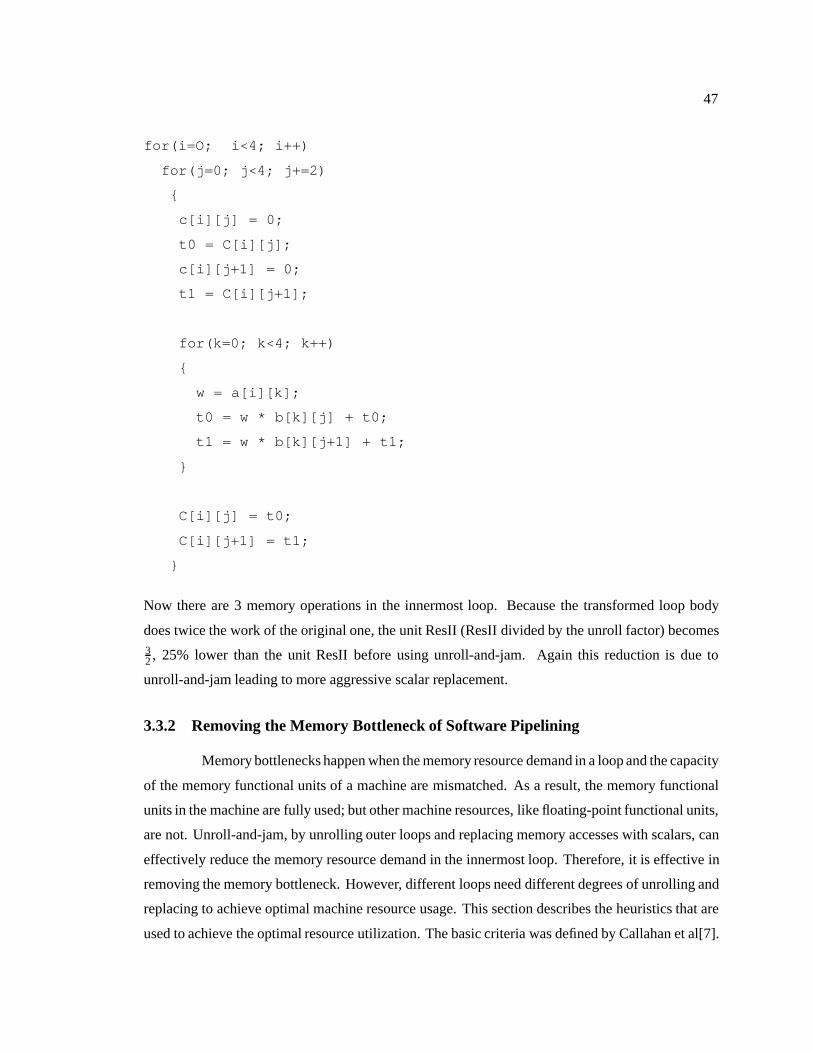
After scalar replacement, the number of memory operations in the innermost loop is decreased to
2 and the ResII is 2 machine cycles. In this manner, unroll-and-jam can remove some memory
operations from the innermost loop by considering multiple iterations of both inner and outer loops
and, thus, increasing the scope of scalar replacement. In this example, unroll-and-jam will find that
the next J loop iteration is c[i][j + 1] = a[i][k] � b[k][j + 1] + t. The loaded value of a[i][k] is
used in both iterations. So by unrolling the J loop once, a load of a[i][k] can be eliminated. After
unrolling the J loop once by unroll-and-jam, the loop becomes:
47
for(i=O; i<4; i++)
for(j=0; j<4; j+=2)
{
c[i][j] = 0;
t0 = C[i][j];
c[i][j+1] = 0;
t1 = C[i][j+1];
for(k=0; k<4; k++)
{
w = a[i][k];
t0 = w * b[k][j] + t0;
t1 = w * b[k][j+1] + t1;
}
C[i][j] = t0;
C[i][j+1] = t1;
}
Now there are 3 memory operations in the innermost loop. Because the transformed loop body
does twice the work of the original one, the unit ResII (ResII divided by the unroll factor) becomes32 , 25% lower than the unit ResII before using unroll-and-jam. Again this reduction is due to
unroll-and-jam leading to more aggressive scalar replacement.
3.3.2 Removing the Memory Bottleneck of Software Pipelining
Memory bottlenecks happen when the memory resource demand in a loop and the capacity
of the memory functional units of a machine are mismatched. As a result, the memory functional
units in the machine are fully used; but other machine resources, like floating-point functional units,
are not. Unroll-and-jam, by unrolling outer loops and replacing memory accesses with scalars, can
effectively reduce the memory resource demand in the innermost loop. Therefore, it is effective in
removing the memory bottleneck. However, different loops need different degrees of unrolling and
replacing to achieve optimal machine resource usage. This section describes the heuristics that are
used to achieve the optimal resource utilization. The basic criteria was defined by Callahan et al[7].
48
Carr and Kennedy gave the algorithm that automatically computes the optimal degree of unrolling
for unroll-and-jam[9]. The criteria is the same when using unroll-and-jam to remove memory
bottlenecks to software pipelining. However, in computing the optimal degree of unrolling, the
effect of overlapping execution needs to be considered.
To illustrate the relation between the resource demand of a loop and the resources available
in a machine, Callahan et al[7] defined the machine balance as
�M =number of memory operations canbe issued per cycle
number of floating � point operations can be issued per cycle
and the loop balance as
�L =number of memory operations in the loop
number of floating � point operations in the loop
[7]. When �L = �M , the memory functional units and the floating-point functional units can all be
fully used. However, when �L � �M , a loop is memory bound and the floating-point functional
units cannot be fully utilized due to the high memory resource demand. For memory bound loops,
�L needs to be reduced to be equal to �M in order to achieve a balanced use of both memory and
floating-point resources. Because of the effect that unroll-and-jam can reduce �L by allowing more
aggressive scalar replacement, we can choose an unroll amount to set �L as close to �M as we wish
for memory-based nested loops.
However, unroll-and-jam leads to a higher register demand for the nested loops since it
jams several iterations together and replaces memory references with scalars. If the register demand
were increased to be higher than the number of available registers, the benefit of unroll-and-jam
would be counteracted by the negative effects of register spilling. So, typically, unroll-and-jam
heuristics also consider the number of registers available in the target machine. If the “optimal"
degree of unrolling requires too many registers, heuristics for unroll-and-jam pick the highest degree
of unrolling that does not require more registers than the machine has.
When using unroll-and-jam to remove the memory bottleneck for software pipelining, the
aim is still to decrease the �L of a memory bound loop to �M . However, the register demand of
software pipelined loops is different from that of a locally or globally scheduled loop. In software
pipelining, the execution of several iterations overlap. This overlapping leads to higher register
demand. For modulo-scheduled loops, a variable may need several registers as a result of kernel
unrolling (Section 2.4.3). Unroll-and-jam needs to consider the overlapping effect of software
pipelining in order to precisely estimate the register pressure of an unrolled loop after software
pipelining.
49
3.4 Estimating the Register Pressure of Unroll-and-Jam
Estimating the register pressure of an unrolled loop after software pipelining is crucial for
using unroll-and-jam with software pipelining. If the estimation is higher than the actual register
pressure, unroll-and-jam will restrict the degree of unrolling heuristically and unroll-and-jam’s
benefit will not be fully exploited. If the estimation is too low, unroll-and-jam will use too many
registers and potentially cripple software pipelining due to register spilling [12].
Two register-pressure estimation methods for modulo scheduled loops, MaxLive and
MinAvg, were described in Section 2.3.4. This section discusses the possible use of these two
estimation methods with unroll-and-jam and proposes a new approach that may be more effective
than simply using MaxLive or MinAvg. To date, the effectiveness of these methods has not been
examined experimentally.
Using MaxLive
MaxLive (described in Section 2.3.4) is the closest estimation to the register demand for
a software pipeline schedule. Rau et al. found that for the loops they tested, the actual register
demand of a schedule was rarely 5 registers more than its MaxLive for a register allocation method
similar to graph-coloring register assignment [34].
Although MaxLive is a fairly precise estimation, it is not practical for unroll-and-jam to
use it. Computing MaxLive can only be done after a software pipeline schedule is found, i.e. after
generating an unrolled loop body and scheduling the generated loop body. It is too time consuming
for unroll-and-jam to try different unrolling based on the value of MaxLive.
Using MinAvg
As described in Section 2.3.4, MinAvg is an estimation that does not depend on any
particular software pipeline schedule. The accuracy of an estimation using MinAvg is affected by
several factors.
The first factor is the accuracy of the predicted II because the computing of MinAvg
depends on a specific II. Due to the fact that the II of a loop cannot be determined until after
software pipelining, the value of II has to be estimated. Fortunately, current leading software
pipelining algorithms can achieve optimal or near-optimal II for most of the loops. So MinII ,
which is the larger of RecII and ResII , can be used as a good estimate of II. Both RecII and
50
ResII can be computed before scheduling. Moreover, RecII can be computed at the source level
if the latencies of the machine are known. The false recurrences caused by the code generation
of a compiler can be ignored since they are not ‘inherent’ recurrences and can be eliminated by
appropriate techniques.
The second factor affecting the computing of MinAvg is how close the MinAvg is to
the actual register demand. Unfortunately, the optimal assumption used in computing MinAvg
sometimes makes it far lower than the actual register pressure in the generated software pipeline
schedule. The basic assumption used in computing MinAvg is that, in a software pipeline schedule,
each variable has a minimum-length lifetime and each register is fully used in every cycle of the
software pipeline. However, resource constraints can lead to longer lifetimes than the minimum
length. Especially for loops in which ResII is much higher than RecII , the lifetime length of
variables can be much longer than the minimum length. Therefore, for loops with relatively high
resource constraints, MinAvg can be quite inaccurate. Moreover, unroll-and-jam increases the
amount of parallelism in the innermost loop. This transformation results in a higher ResII relative
to RecII . So MinAvg is probably not a precise estimation for unroll-and-jam.
Using MinDist
MinDist can be computed once the II is known. As stated previously, II can be esti-
mated with good accuracy. Given II, MinDist gives the minimum lifetime of each variable. This
information can be very helpful in estimating the register pressure.
Without considering the overlapping effect of software pipelining, the register pressure
of the unrolled loop can be precisely estimated using the algorithm given by Carr and Kennedy
[9]. So if the additional register demand caused by the overlapping effect is known, the register
pressure after software pipelining can be precisely estimated. MinDist can be used to compute the
effect of overlapping on register pressure for modulo scheduled software pipeline schedules. The
overlapping in software pipelining requires additional registers only when the lifetime of a register
is longer than II. MinDist provides the lower bound of the lifetime of each variable and this lower
bound can serve as an estimation directly. If the minimum lifetime of a variable is L, the variable
adds d LII e � 1 registers to the register pressure in the software pipeline schedule.
The disadvantage of using MinDist is that the resource constraints can lead to register
lifetimes much longer than their minimum value in the unrolled loops. However, using MinDist is
51
more accurate than using MinAvg because the prediction using MinDist does not assume an optimal
register usage. MinDist is only used to compute additional registers needed due to the overlapping
of software pipelining.
3.5 Comparing unroll-and-jam with Other Loop Transformations
This section describes the advantages of unroll-and-jam, with regard to software pipelin-
ing, over the two other popular loop transformations, namely tree height reduction and loop inter-
change.
3.5.1 Comparison with Tree-Height Reduction
Tree-height reduction (THR) is a general technique that considers the computation carried
by the loop as a computing tree and restructures the computing tree so that more computations can
be parallelized and the height of the tree can be reduced[23]. Tree-height reduction can be applied to
not only nested loops but also single loops. It generally involves innermost loop unrolling and back-
substitution. Tree-height reduction has recently been used and evaluated on ILP architectures[38]
and in modulo scheduling [26].
Both unroll-and-jam and THR increase the amount of parallelism in the innermost loop.
However, the sources of the increased parallelism are totally different. Unroll-and-jam transforms a
nested loop and puts parallelism from outer loops into the innermost loop, whereas THR transforms
the computation in the innermost loop and exposes more parallelism from within the innermost
loop. Each method deals with different sources of parallelism and each can be used with the other
to obtain both benefits without problem.
The major advantage of THR is that it can be applied to any loops whereas unroll-and-jam
can only be used for nested loops. Although THR is not specifically designed for nested loops, it
may exploit cross-loop parallelism by interchanging the nested loop. However, as described in the
next section, there are two shortcomings with the use of loop interchange: loop interchange is not
always legal, and it can lead to poor cache performance.
Unroll-and-jam, however, can exploit cross-loop parallelism without difficulties caused
by loop interchange. The amount of cross-loop parallelism is quite large. For architectures with
high degree of hardware parallelism, exploiting cross-loop parallelism is essential. Compared to
THR, unroll-and-jam can more effectively reduce resource constraints in the transformed loop.
52
The unrolling performed by both unroll-and-jam and THR brings in more computations that allow
traditional optimization to reduce more operations. But unroll-and-jam can enhance chances for
scalar replacement across loop boundaries. THR, since it limits its scope only to the innermost
loop, cannot achieve the benefit of optimization across loops. Therefore, unroll-and-jam is more
effective in reducing resource constraints for software pipelining than THR.
Unroll-and-jam has another advantage over THR because the effect of unroll-and-jam on
RecII can be accurately predicted and the degree of unrolling can be determined before transforma-
tion. However, THR cannot predict the resulting RecII before transformation, and, thus, the degree
of innermost loop unrolling cannot be optimally determined.
3.5.2 Comparison with Loop Interchange
Loop Interchange can switch an outer loop to be the innermost loop. To minimize
the recurrence in the innermost loop, loop interchange should switch the loop that has the least
recurrence to be the innermost loop. By doing so, loop interchange may decrease the recurrence in
the innermost loop without increasing the size of the innermost loop. However, it may not be legal
to perform loop interchange. Even when loop interchange can be performed freely, it still has three
disadvantages compared with unroll-and-jam.
The first disadvantage of loop interchange is that it may not always eliminate the effect
of recurrence in the innermost loop. If a multiple-nested loop does not have a loop that has no
recurrence, loop interchange cannot eliminate the effect of the recurrence in the innermost loop as
unroll-and-jam can. The unit RecII will be the same as the lowest RecII in all loops, but it cannot
be reduced further. The second disadvantage of loop interchange is that by changing the order of
the loop, cache performance may be worsened significantly. Poor cache performance will cause a
much higher register pressure in software pipelining.
53
Chapter 4
Improving Software Pipelining with
Memory Reuse Analysis
The deep memory hierarchy in today’s microprocessors causes uncertain latencies for
memory operations. In the past, software pipelining algorithms either assumed that each memory
operation takes the shortest possible time to finish or they assumed that each memory operation
takes the longest possible time to finish. This chapter shows that both assumptions are undesirable
because they each degrade software pipelining’s performance. The behavior of a memory operation
can and should be predicted by using a compiler technique called memory reuse analysis. By taking
advantage of predictions provided by such analysis, software pipelining should be able to achieve a
much better performance than that possible with either optimistic (all memory operations take the
shortest time possible) or pessimistic (all memory operations require the longest latency possible)
assumptions.
4.1 Memory Hierarchy
The speed of today’s microprocessors is much greater than the speed of today’s memory
systems. Over the past ten years, the processor speed has increased at a higher rate than that of
the memory system. As a result, today’s machines have a significant gap between CPU speed and
memory speed. Although an integer addition typically takes only one machine cycle in the CPU,
a load from the main memory may take 30 cycles. To reduce the average time required to load a
value from main memory to CPU, cache is used in all modern machines to serve as a buffer between
the processor and the main memory. Cache is much faster than the main memory. A load from a
54
first level (usually on-chip) cache normally takes only 2 to 3 machine cycles. However, cache is
much smaller than main memory and thus, it is sometimes impossible to have all the data needed
by a program fit into the cache.
Memory hierarchy is the term to describe current memory systems that consist of different
levels of data storage. In such a hierarchy, registers are the fastest, but smallest ‘memory’. Main
memory is the slowest, but largest. Cache has a speed and a size in between. Most recent machines
use a multiple-level cache, i.e. a small, fast, on-chip cache and a larger, slower, off-chip cache.
With the speed difference between the processor and the main memory getting larger, the memory
hierarchy necessarily becomes deeper to maintain sufficient memory speeds.
The deep memory hierarchy causes significant uncertainty in the time needed for a
memory operation. During execution, some data come from cache and some from main memory.
The memory latency, which is the time needed for a memory load or store, varies drastically
depending upon whether the data comes from cache or from main memory. A load or store from
the fast first-level data cache is called a cache hit and a load or store from a second-level cache or
main memory is called a cache miss. The latency of a cache hit and the latency of a cache miss
normally differs by a factor of 10 or more.
4.2 Memory Reuse Analysis
Memory reuse analysis is a compiler technique used to predict the cache behavior by
analyzing the reuse of data in a program. It predicts whether a memory load or store is a cache hit
or a cache miss. Cache memories are based upon the assumption that most data is used multiple
times. When data are loaded from the main memory, they are placed in the cache. So if the data
is used again before it must be removed from the cache (to make room for other data), the second
load of the data is a cache hit. The cache concept, and indeed the entire memory hierarchy, reduces
the average memory access time significantly because programs exhibit locality.
Programs actually exhibit two types of locality. First, data that have been used “recently"
in a program are likely to be reused again soon. Such multiple use of the same data is called temporal
locality and, likewise, the reuse of previously loaded data is called temporal reuse. In addition to
temporal locality, programs tend to use data which are “close together" such as contiguous elements
of an array. This locality is called spatial locality and leads to the term spatial reuse when spatial
locality yields a cache hit. In terms of cache behavior, temporal reuse occurs when, after data is
loaded from the main memory, the same data is loaded again. At the first load, the data will be
55
moved to the cache; therefore the second load will be a cache hit. Caches make use of spatial reuse
in that when one location is used, data in nearby locations are loaded as well. When the first data is
loaded, a whole block of data containing the loaded data is loaded into the cache. A block contains
a group of adjacent data. So along with the data initially accessed, other data near the initial data
are placed in the cache. When a subsequent memory operation accesses data near the initial data
(spatial reuse), access will be a cache hit as well.
Let’s considering the following loop of matrix multiply. There are four memory references
in the innermost loop. The two references ofC[i] have temporal locality because the same data,C[i],
is accessed every time in the innermost loop. The other two memory references access different
data in every iteration. Let’s assume the array A andB are stored in row-major order. Then memory
access A[i; j] in each iteration has spatial reuse because it is near the previous A[i; j] in the last
iteration. Memory access B[j; i] has neither temporal reuse nor spatial reuse because B[j; i] in each
iteration is a long distance in memory from the access in the previous iteration.
for (i=0; i<M; i++)
for (j=0; j<M; j++)
{
C[i] = C[i] + A[i,j]*B[j,i];
}
Memory reuse analysis examines each memory operation to see if it has spatial reuse,
temporal reuse or neither of the two. One relatively simple cache prediction scheme assumes that
any static operation that exhibits reuse (as determined by compile-time analysis) will always yield
a cache hit and that any static operation that cannot be demonstrated by conservative compile-time
analysis to exhibit reuse is always a cache miss. There are currently two popular compile-time
analysis models that have been used to identify memory reuse; one is based upon sophisticated
dependence analysis[11] and the other uses a linear algebra model [46]. The reader should refer to
those resources for algorithm details.
4.3 Removing Hardware Misuse with Memory Reuse Analysis
As discussed previously, the problem of uncertainty latencies is rooted in the deep mem-
ory hierarchy of modern microprocessors. However, memory reuse analysis can help solve the
56
uncertain-latency problem by predicting cache hits and misses. Without using memory reuse anal-
ysis, a compiler cannot have the precise knowledge of the latencies of memory operations. When a
latency of a memory operation is unknown to a compiler, the compiler must either assume that it is a
cache hit or a cache miss. Some compilers assume that all memory loads are cache hits (all-cache-
hit assumption) and some treat all memory loads as cache misses (all-cache-miss assumption).
The all-cache-hit assumption under-estimates the latency of a cache miss and the all-cache-miss
assumption over-estimates the latency of a cache hit. Both assumptions are imprecise, as the latency
difference between cache-hit loads and cache-miss loads can be a factor of ten.
This section will examine both the all-cache-hit and the all-cache-miss assumption used
in software pipelining and show that both assumptions can significantly degrade the performance
of software pipelining. When memory reuse analysis is used, these degradations can be avoided.
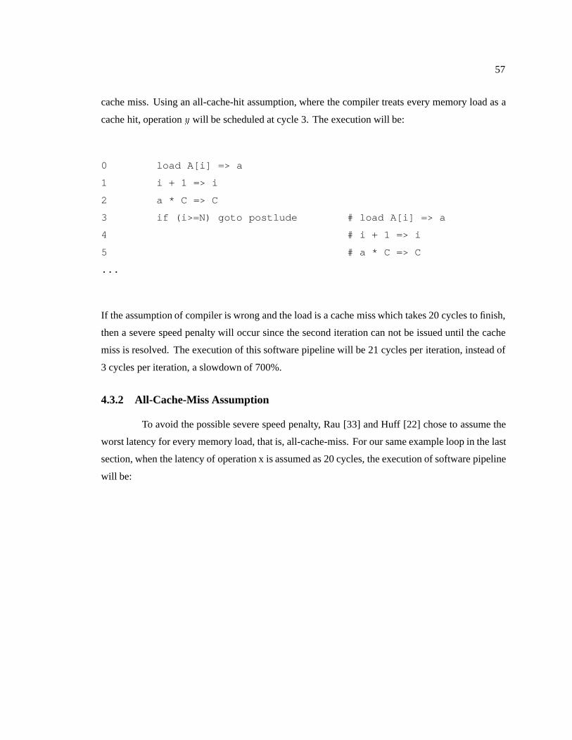
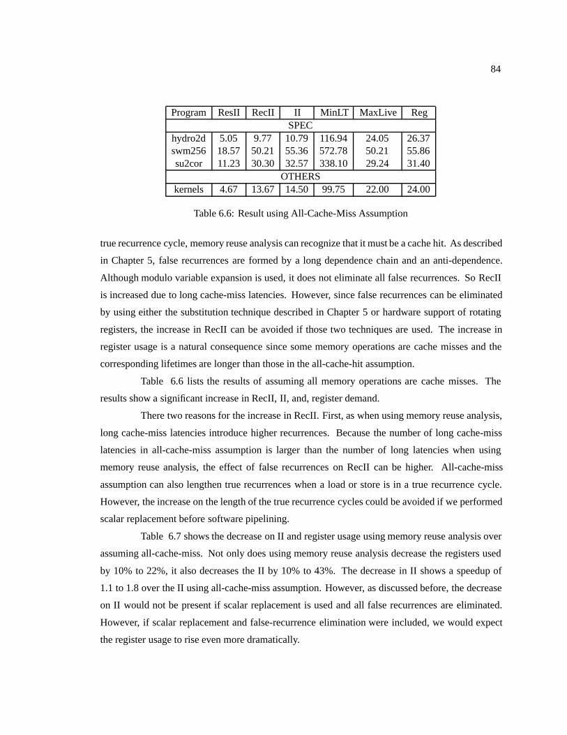
4.3.1 All-Cache-Hit Assumption
Consider an example loop on a machine where a cache hit takes two cycles, a cache miss
takes twenty cycles and other operations take two cycles.
for (i=0; i<N; i++)
{
C += A[i];
}
Assume the II of the generated software pipeline is 3 cycles and the schedule for one iteration is,
Operation Cycle
x 1 load A[i] => t1
u 2 i + 1 => i
v 4 if (i>=N) goto postlude
y t t1 * C => C
Note that operation y, scheduled at cycle t, depends on the assumed latency of the load of A[i]. If
the compiler assumes the load is a cache hit, t will be 3; otherwise, t is 21 assuming the load is a
57
cache miss. Using an all-cache-hit assumption, where the compiler treats every memory load as a
cache hit, operation y will be scheduled at cycle 3. The execution will be:
0 load A[i] => a
1 i + 1 => i
2 a * C => C
3 if (i>=N) goto postlude # load A[i] => a
4 # i + 1 => i
5 # a * C => C
...
If the assumption of compiler is wrong and the load is a cache miss which takes 20 cycles to finish,
then a severe speed penalty will occur since the second iteration can not be issued until the cache
miss is resolved. The execution of this software pipeline will be 21 cycles per iteration, instead of
3 cycles per iteration, a slowdown of 700%.
4.3.2 All-Cache-Miss Assumption
To avoid the possible severe speed penalty, Rau [33] and Huff [22] chose to assume the
worst latency for every memory load, that is, all-cache-miss. For our same example loop in the last
section, when the latency of operation x is assumed as 20 cycles, the execution of software pipeline
will be:
58
0 load A[i] => a1
1 i + 1 => i
2
3 if (i>=N) goto # load A[i] => a2
4 # i + 1 => i
5
6 # if (i>=N) goto # load A[i] => a3
... ... ...
20 a1 * C => C
21 # a2 * C => C
22 # a3 * C => C
This software pipeline, when at its full speed, completes one iteration every three cycles. Notice
the variables a1, a2, etc are introduced by kernel unrolling because the lifetime of the loaded value
is longer than II. The compiler assumes that the load takes 20 cycles, consequently, it reserves 21
cycles of lifetime for the loaded value. This long lifetime needs 7 registers. However, if the load is
a hit, only three cycles of lifetime and one register are needed. So the over-estimation costs 6 more
registers for this example.
4.3.3 Using Memory Reuse Analysis
As described in the previous sections, when the all-cache-hit assumption under-estimates
the latency of cache-miss loads, the speed of the software pipeline is severely degraded; when the
all-cache-miss assumption over-estimates the latency of cache-hit loads, the software pipeline uses
many more registers than needed. By using memory reuse analysis, software pipelining should
neither over-estimate nor under-estimate the latency of memory operations. So the degradation of
the software pipeline speed and the unnecessary use of registers can be avoided with memory reuse
analysis. In practice, of course, memory reuse analysis cannot guarantee to identify each cache hit
and cache miss. However, it should yield improved software pipelining when compared to either
an all-cache-hit or an all-cache-miss policy.
59
Chapter 5
Improving Modulo Scheduling
Modulo scheduling is a effective scheduling technique for software pipelining. Experi-
mental results have shown that it can achieve near-optimal II for most benchmark loops[33] [4].
This chapter discusses two enhancements to modulo scheduling. Previously, modulo scheduling
could not eliminate all false recurrences without the hardware support of rotating registers. Section
1 proposes a compiler algorithm that can efficiently eliminate the effect of all false recurrences for
conventional architectures. Section 2 describes a faster method of computing RecII than is currently
used in practice.
5.1 Eliminating False Recurrences
As described in Chapter 1, anti and output dependences are called false dependences
because they can be removed by appropriate variable renaming without changing program semantics.
Therefore, the recurrence cycle in a loop that contains anti or output dependences is not a true
recurrence. I call it a false recurrence. Thus, a true recurrence is a loop-carried dependence cycle
in which each edge is a true dependence. Various software and hardware methods have been used
to eliminate the effect of false dependences and recurrences.
Hardware renaming is one method of eliminating anti-dependences that has been used
for a long time[41]. In the realm of hardware renaming, an anti-dependence is known as a WAR
(write-after-read) hazard. When the hardware detects a WAR hazard, it can copy the value to a
temporary and let the second operation proceed without waiting for the first operation to finish. The
hardware then forwards the copied value to the first operation when needed. In this manner, the
WAR hazard is eliminated at the cost of an additional location necessary for the temporary.
60
Compilers have also made attempts to eliminate anti and output dependences by “renam-
ing". In a manner similar to hardware renaming, compilers assign additional temporaries to remove
possible anti and output dependences. One popular method of compiler renaming is the use of
static single assignment (SSA)[14]. In SSA, each produced value uses a separate variable so that
the reuse of variables can be eliminated.
However, when software pipelining, neither traditional hardware or software renaming
can completely eliminate false recurrences in a loop. When the execution of different iterations
overlaps, the use of a value in a previous iteration may occur long after a define in a later iteration.
Thus, the hardware does not even know there is a use in the previous iteration before the define of
the current iteration. Traditional software renaming does not rename a value for each iteration. If
a value a is defined in a loop body, traditional software renaming does not give a different location
to the a produced in each iteration. Therefore, false recurrences may happen due to the reuse of the
location of a by multiple iterations.
If a value is defined in a loop, a complete renaming would require a separate variable for
each iteration of the loop. This type of renaming was used in vectorizing compilers[24], where
the defined variable is expanded into a higher degree of array. However, this type of renaming is
too expensive to be practical in conventional machines. One method of special hardware support,
namely rotating registers (RR), has been suggested [13] [36]. Rau et al. used RRs for modulo
scheduled loops [34]. In a machine with support for RRs, the index of registers are shifted every II
cycles. This shifting produces the effect that each II uses a different set of registers and the reuse
of the same location can be avoided. Although RRs can eliminate all false recurrences caused by
the reuse of variables, it is an expensive hardware feature that is not available on any of today’s
machines.
Lam [25] proposed a software solution to this problem called Modulo Variable Expansion
(MVE). The advantage of MVE is that it requires no hardware support not found on conventional
architectures. MVE identifies all variables that are reproduced at the beginning of each iteration
and removes the loop carried dependence between the use and the define of each reproduceable
variable. After modulo scheduling, MVE unrolls the kernel as appropriate to avoid any lifetime
overlapping itself (see Section 2.4.3).
However, as described in the next section, modulo variable expansion is incomplete
because it only applies to a subset of loop-carried anti-dependences. Other loop-carried dependence
and loop-independent anti-dependences are ignored. The remaining anti-dependences may still
cause false recurrences that cannot be eliminated by MVE.
61
;use Xnuse A
;use Xnuse A use A
def A
def A
use A
chain
dependence
...
use Xk-1; def Xk
use A; def X1
def A
use Xk; def Xk+1
use Xn-1; def Xn
...
loop-invariant
b) use-before-define false recurrence
...
use X1; def X2
use A; def X1
use Xn-1; def Xn
def A
loop-carried
anti
dependence
a) use-after-define false recurrence
dependencechain
iteration iteration
intra- inter-
anti dependence
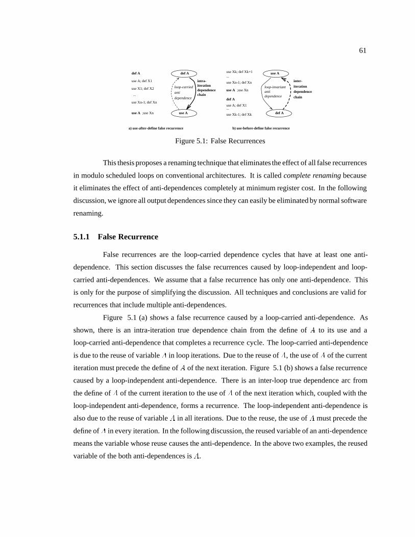
Figure 5.1: False Recurrences
This thesis proposes a renaming technique that eliminates the effect of all false recurrences
in modulo scheduled loops on conventional architectures. It is called complete renaming because
it eliminates the effect of anti-dependences completely at minimum register cost. In the following
discussion, we ignore all output dependences since they can easily be eliminated by normal software
renaming.
5.1.1 False Recurrence
False recurrences are the loop-carried dependence cycles that have at least one anti-
dependence. This section discusses the false recurrences caused by loop-independent and loop-
carried anti-dependences. We assume that a false recurrence has only one anti-dependence. This
is only for the purpose of simplifying the discussion. All techniques and conclusions are valid for
recurrences that include multiple anti-dependences.
Figure 5.1 (a) shows a false recurrence caused by a loop-carried anti-dependence. As
shown, there is an intra-iteration true dependence chain from the define of A to its use and a
loop-carried anti-dependence that completes a recurrence cycle. The loop-carried anti-dependence
is due to the reuse of variable A in loop iterations. Due to the reuse of A, the use of A of the current
iteration must precede the define of A of the next iteration. Figure 5.1 (b) shows a false recurrence
caused by a loop-independent anti-dependence. There is an inter-loop true dependence arc from
the define of A of the current iteration to the use of A of the next iteration which, coupled with the
loop-independent anti-dependence, forms a recurrence. The loop-independent anti-dependence is
also due to the reuse of variable A in all iterations. Due to the reuse, the use of A must precede the
define ofA in every iteration. In the following discussion, the reused variable of an anti-dependence
means the variable whose reuse causes the anti-dependence. In the above two examples, the reused
variable of the both anti-dependences is A.
62
To eliminate a false recurrence caused by a loop-carried anti-dependence, we must be
able to rename the reused variable so that the define of the next iteration can use a different variable
than the use of the current iteration and the loop-carried anti-dependence can be eliminated. To
remove a false recurrence caused by a loop-independent anti-dependence, the renaming of the
reused variable should make the define and the use in each iteration use two different variables so
that the loop-independent anti-dependence can be removed.
5.1.2 Modulo Variable Expansion
To eliminate the effect of certain false recurrences, Lam proposed a compiler renaming
technique called Modulo Variable Expansion[25]. This section gives a detailed description of MVE
and shows why MVE is neither complete nor efficient for eliminating all false recurrences. MVE
can eliminate the anti-dependence that satisfies,
� it is a loop-carried anti-dependence, and,
� the value defined in the reused variable is reproduceable in each iteration. (A value that is
reproduceable in a iteration means that the value does not rely on any value computed by
previous iterations.)
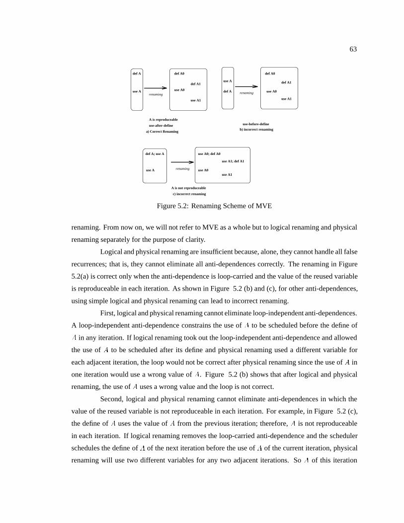
Figure 5.2(a) shows the effect of MVE. The renaming of MVE can be seen as two steps. First,
before scheduling, MVE prunes the loop-carried anti-dependence. Without the restriction of the
loop-carried anti-dependence, the scheduler can schedule the use of A of the current iteration after
the define of A of the next iteration. When this happens, the lifetime of A is longer than II and must
overlap with itself in the kernel. In the second step, performed after scheduling, MVE renames A
into separate registers so that no lifetime of the renamed As can overlap with itself. The second step
is also called kernel unrolling because the renaming requires unrolling of the kernel. (The method
of kernel unrolling is described in Section 2.4.3.) In Figure 5.2(a), the variable A is renamed into
two variables so that the define ofA of the next iteration would not affect the use ofA of the current
iteration. Thus, the loop-carried anti-dependence is removed and so is the false recurrence cycle.
I call the first step of MVE, which is the pruning of the anti-dependence, logical renaming,
since this step tells the scheduler that the variable can be renamed; I call the second step of MVE,
where the variable is physically renamed into separate variables, physical renaming. Logical
renaming enables scheduling to ignore the anti-dependence, which may lead to lifetimes longer
than II; physical renaming avoids the overlapping of the long lifetimes that may result from logical
63
renaming
def A
use A
def A; use A
use A renaming
use A
def A
b) incorrect renaming
use-before-define
A is not reproduceable
c) incorrect renaming
renaming
A is reproduceable
use-after-define
a) Correct Renaming
def A1
use A1
def A1
use A1
use A1; def A1
use A1
def A0
use A0
def A0
use A0
use A0; def A0
use A0
Figure 5.2: Renaming Scheme of MVE
renaming. From now on, we will not refer to MVE as a whole but to logical renaming and physical
renaming separately for the purpose of clarity.
Logical and physical renaming are insufficient because, alone, they cannot handle all false
recurrences; that is, they cannot eliminate all anti-dependences correctly. The renaming in Figure
5.2(a) is correct only when the anti-dependence is loop-carried and the value of the reused variable
is reproduceable in each iteration. As shown in Figure 5.2 (b) and (c), for other anti-dependences,
using simple logical and physical renaming can lead to incorrect renaming.
First, logical and physical renaming cannot eliminate loop-independent anti-dependences.
A loop-independent anti-dependence constrains the use of A to be scheduled before the define of
A in any iteration. If logical renaming took out the loop-independent anti-dependence and allowed
the use of A to be scheduled after its define and physical renaming used a different variable for
each adjacent iteration, the loop would not be correct after physical renaming since the use of A in
one iteration would use a wrong value of A. Figure 5.2 (b) shows that after logical and physical
renaming, the use of A uses a wrong value and the loop is not correct.
Second, logical and physical renaming cannot eliminate anti-dependences in which the
value of the reused variable is not reproduceable in each iteration. For example, in Figure 5.2 (c),
the define of A uses the value of A from the previous iteration; therefore, A is not reproduceable
in each iteration. If logical renaming removes the loop-carried anti-dependence and the scheduler
schedules the define of A of the next iteration before the use of A of the current iteration, physical
renaming will use two different variables for any two adjacent iterations. So A of this iteration
64
cannot read the A of the previous iteration since the adjacent iterations use two different variables
for A. The schedule after logical and physical renaming is incorrect.
Not only are simple logical and physical renaming insufficient, they also are inefficient
in terms of register usage because logical renaming blindly prunes all applicable anti-dependences.
When the false recurrences caused by an anti-dependence are not the limiting constraint for II,
they need not be eliminated. So, preserving such anti-dependence will not affect the performance
of software pipelining. However, if we unnecessarily prune the anti-dependence by blind logical
renaming, scheduling and physical renaming may unnecessarily use multiple registers for the
variable; therefore, software pipelining may use more registers than necessary.
To show the possible over-use of registers by logical renaming, let’s consider Figure 5.2
(a) again. If the false recurrence caused by the loop-carried anti-dependence is not more restrictive
than other software pipelining constraints, the minimum lifetime ofA fits into II cycles. The logical
renaming is unnecessary since we can schedule the use of A of the current iteration before the
define of A of the next iteration without hurting the value of II. Moreover, the preserving of the
anti-dependence would force the scheduler to schedule the A’s lifetime to be less than II; therefore,
only one register is needed for A. However, if logical renaming blindly prunes this loop-carried
anti-dependence, the scheduler may create a lifetime of A that is longer than II. Subsequently,
physical renaming would require more than one register for A and unnecessarily increase the
register pressure.
5.1.3 Define-Substitution
Simple logical and physical renaming cannot eliminate anti-dependences that either are
loop-independent or caused by a reused variable that is not reproduceable. This section proposes a
technique that performs substitution to the define of the reused variable so that, after substitutions,
logical and physical renaming can eliminate those two types of anti-dependences correctly. I call
this substitution technique define-substitution. The idea is to substitute the anti-dependences that
cannot be handled by logical and physical renaming with anti-dependences that can be eliminated by
logical and physical renaming. Define-substitution consists of pre-substitution and post-substitution.
Pre-substitution is used on loop-independent anti-dependences; post-substitution is applied to anti-
dependences in which the reused variable is not reproduceable. After pre-substitution and post-
65
substitution, the original anti-dependences are changed to loop-carried dependences where the
reused variable is reproduceable 1.
In order to substitute loop-independent anti-dependences with desirable loop-carried anti-
dependences, pre-substitution copies the value of the reused variable before any of its use in each
iteration. Figure 5.3 (a) shows the effect of pre-substitution on a loop-independent anti-dependence.
Pre-substitution copies the value of the reused variable, A, to a substituting variable A0 and changes
the use of A to the use of A0. After substitution, the anti-dependence from the use of A to the define
of A is changed to a loop-carried anti-dependence from the use of A0 to the define of A0. A0 is
reproduceable in each iteration since the recurrence existing between the define of A and the define
of A0 ensures that A0 has a correct value in each iteration. Because the new anti-dependence is
loop-carried and A0 is reproduceable, logical and physical renaming can be performed onA0 and the
false recurrence can be eliminated. In pre-substitution, the copying should be done before any use
of A; only the uses of A that occur before the define of A can be changed to use A0. The placement
of a copy operation in pre-substitution is the same location where software renaming, SSA, would
put a � node. This � node merges of the value coming in from the outside of the loop and the value
generated inside the loop. If the � node is implemented by a copy operation, then SSA can have the
effect of pre-substitution.
Post-substitution is used on anti-dependences that are caused by the reuse variable that is
not reproduceable. As shown in the example in Figure 5.3 (b), post-substitution copies the reused
variable, A, to a substituting variable A0 after the define of A, and changes the use of A toA0. After
substitution, the anti-dependence between the use of A0 and the define of A0 is loop-carried, and A0
is reproduceable. So logical and physical renaming can be performed onA0 and the anti-dependence
can be removed. In post-substitution for a loop-carried dependence, the copying of A to A0 should
be done after the define of A but before any of its uses; only the uses of A that are after the define
of A may can be changed to use A0. Post-substitution for any loop-independent anti-dependence is
unnecessary since after pre-substitution, the reused variable must be reproduceable.
As define-substitution inserts a copy of the reused variable, a true and an anti-dependence
are also inserted into the DDG. We must not allow these dependences to be inserted into any
existing recurrences because they will increase the length of the host recurrence. Let’s consider
Figure 5.1 (a) for an example. If A is not reproduceable, post-substitution copies it to A0 and
changes use A; def X1 to use A0. This change lengthens the dependence chain from the define
1Here we expand the concept of reproduceable to include those values produced in remaining recurrences cycles afterlogical renaming. They are reproduceable in each iteration due to the constraint imposed by the recurrences.
66
Pre-substitution
A’ <- A
use A’
def A use A’0
A’0 <-A
def AA’1<-A
def A
use A’1
renaming
use A
def A
use-before-define
a) Pre-substitution and Renaming
def A; use A
A’ <- A
use A’renaming
def A; use A
A’0 <- A
use A’0
def A; use A
A’1 <- A
use A’1
def A; use A
use A
b) Post-substitution and Renaming
use-after-define
Post-substitution
Figure 5.3: Pre and Post-Substitution
of A to the use of A. If the define and the use are in a true recurrence cycle, this change would
lengthen the true recurrence cycle as well. To avoid this result, we must prohibit substituting a use
of A if the use is in a true recurrence (called host recurrence) with the define of A. Although this
restriction preserves the anti-dependence, it does not affect the effect of define-substitution because
the preserved anti-dependence cannot cause false recurrences longer than the host true recurrence.
However, a practical concern arises in the implementation of this restriction: how do we know if
the define and the use of a reused variable is in a true recurrence cycle? The actual problem is more
complicated because, for the purpose of efficiency, we may preserve some false recurrences in the
loop and we must consider those false recurrences as well as all true recurrences. This problem
can be solved; but we delay the answer to the next section. With the restriction described above,
define-substitution will cause no additional recurrence to the loop body.
As shown in the above discussion, define-substitution changes the anti-dependences that
cannot be handled by logical and physical renaming so that after define-substitution, all anti-
dependences can be eliminated by logical and physical renaming. Although define-substitution
inserts copies into the loop body, it does not create higher recurrences. Therefore, with define-
substitution, the effect of all false recurrences can be eliminated for modulo scheduling.
5.1.4 Restrictive Renaming
The elimination of false recurrences increases register demand since both define-substitution
and renaming require additional registers. To minimize the register cost of eliminating false re-
67
currences, we must avoid any unnecessary uses of define-substitution and renaming. This section
describes a technique that can identify those false recurrences that need to be eliminated. By
applying define-substitution and renaming only to those necessary false recurrences, unnecessary
register cost can be avoided. The technique is called restrictive renaming since it restricts the
define-substitution and renaming. Similarly we call the blind logical and physical renaming used
by MVE unrestrictive renaming.
To minimize the use of define-substitution and renaming, we want to eliminate only false
recurrences that are more restrictive than other software pipelining constraints, namely constraints
due to true recurrences and constraints of limited resources in the target machine. I call the
lowerbound on II due to true recurrences TrueII. Thus, the larger of the TrueII and ResII, TrueMII,
is the lowerbound II due to everything but false recurrences. The purpose of restrictive renaming is
to achieve TrueMII while eliminating a minimum number of false recurrences. Therefore, only false
recurrences with a length greater than TrueMII need be eliminated. The problem then, becomes,
finding all false recurrences and determining the length of each false recurrence.
I will categorize false recurrences by the number of anti-dependences in the dependence
cycle. False recurrences that contain only one anti-dependence are denoted as �1-recurrences.
Similarly, false recurrences that contain n anti-dependences are denoted as �n-recurrences. An
�1-recurrence cycle consists of a true dependence chain with a single anti-dependence. Let’s
assume that we know the length of the longest true dependence chain between any two DDG
nodes. The length of each �1-recurrence can be obtained by checking every anti-dependence: if
an anti-dependence is from node x to y, the longest length of the �1-recurrence caused by this
anti-dependence is the length of the longest true dependence chain from y to x plus the timing of
the anti-dependence.
The length of the longest true dependence chain between any two nodes can be found by
computing the longest path problem and considering only true dependences in the DDG. (The timing
of loop-carried dependences in the DDG is computed using II equal to TrueMII.) The computing
of the longest path problem can be done by changing the sign of edges and computing the shortest
path problem.
Using TrueMII and considering only true dependences, we can compute the longest path
between any two nodes and represent it with an adjacency matrix. We call this matrix TrueDist0.
The longest true dependence chain from node x to y is the value in TrueDist0[x; y]. If there is no
path from x to y, TrueDist0[x; y] is �1. Thus, if an anti-dependence a is from node y to x, the
68
length of the longest �1-recurrence caused by a is