remote sensing

Letter

Improving the Altimeter-Derived Surface CurrentsUsing Sea Surface Temperature (SST) Data:A Sensitivity Study to SST Products

Daniele Ciani 1,* , Marie-Hélène Rio 2, Bruno Buongiorno Nardelli 3 , Hélène Etienne 4

and Rosalia Santoleri 1

1 Consiglio Nazionale delle Ricerche, Istituto di Scienze Marine (CNR-ISMAR), 00133 Rome, Italy;daniele.ciani@cnr.it (D.C.); rosalia.santoleri@cnr.it (R.S.)

2 European Space Agency, European Space Research Institute (ESA-ESRIN), 00044 Frascati, Italy;Marie-Helene.RIO@esa.int

3 Consiglio Nazionale delle Ricerche, Istituto di Scienze Marine (CNR-ISMAR), 80133 Naples, Italy;bruno.buongiornonardelli@cnr.it

4 Collecte Localisation Satellites (CLS), 31520 Ramonville St-Agne, France; hetienne@groupcls.com* Correspondence: daniele.ciani@cnr.it

Received: 23 March 2020; Accepted: 15 May 2020; Published: 17 May 2020�����������������

Abstract: Measurements of ocean surface topography collected by satellite altimeters providegeostrophic estimates of the sea surface currents at relatively low resolution. The effective spatial andtemporal resolution of these velocity estimates can be improved by optimally combining altimeterdata with sequences of high resolution interpolated (Level 4) Sea Surface Temperature (SST) data,improving upon present-day values of approximately 100 km and 15 days at mid-latitudes. However,the combined altimeter/SST currents accuracy depends on the area and input SST data considered.Here, we present a comparative study based on three satellite-derived daily SST products: the RemoteSensing Systems (REMSS, 1/10◦ resolution), the UK Met Office OSTIA (1/20◦ resolution), and theMultiscale Ultra-High resolution SST (1/100◦ resolution). The accuracy of the marine currentscomputed with our synergistic approach is assessed by comparisons with in-situ estimated currentsderived from a global network of drifting buoys. Using REMSS SST, the meridional currents improveup to more than 20% compared to simple altimeter estimates. The maximum global improvementsfor the zonal currents are obtained using OSTIA SST, and reach 6%. Using the OSTIA SST also resultsin slight improvements ('1.3%) in the zonal flow estimated in the Southern Ocean (45◦S to 70◦S).The homogeneity of the input SST effective spatial resolution is identified as a crucial requirement foran accurate surface current reconstruction. In our analyses, this condition was best satisfied by thelower resolution SST products considered.

Keywords: sea surface temperature; ocean currents; altimetry; earth observations synergy

1. Introduction

Oceanic currents are a key factor in modulating both the short-term and climatological dynamicsof the ocean–atmosphere system. On a large scale, their monitoring is needed to evaluate themeridional transport of heat and salt and better predict ocean thermohaline circulation variabilityand changes [1]. At the oceanic meso- to sub-mesoscales, the characterization of the marinecurrents is also crucial. Mesoscale eddies are non-stationary and energetic recirculation featureswith horizontal scales of 10 to 100 km and can persist on timescales of weeks to months. They canmigrate for several miles carrying heat, salt and nutrients, and their perturbations can drive intensevertical exchanges. Submesoscale features like eddies, fronts and filaments are characterized by

Remote Sens. 2020, 12, 1601; doi:10.3390/rs12101601 www.mdpi.com/journal/remotesensing

Remote Sens. 2020, 12, 1601 2 of 16

spatial-temporal scales of 0.1 to 10 km and hours to days. Such small-scale, short-lived features canalso generate significant heterogeneities in both horizontal and vertical velocities, affecting the local 3Dtransport properties [2–8]. Interestingly, it was demonstrated that even weak geostrophic flows play asignificant role in the transport processes, mostly due to their persistence on synoptic to seasonal timescales [9–12].

At the sea surface, the ocean current monitoring also serves several societal and environmentalapplications, including ship routing, safety and rescue activities and the monitoring of floatingpollutants like oil slicks and plastic debris [13,14]. All these applications necessitate an accurate,high spatial-temporal resolution monitoring of the upper layer oceanic currents.

Since the early 1990s, radar altimeters onboard satellites have been providing indirect measuresof the marine surface circulation at a global scale [15]. This is achieved by measuring the Sea SurfaceHeight (SSH) relative to an equipotential surface (the so-called geoid) and inferring the surface motionvia the geostrophic approximation [16]. This system has intrinsic limitations related to the sampling ofSSH and to the approximation considered in the retrieval. Indeed, only larger mesoscale geostrophicprocesses can be described with this approach [17–19].

The direct estimate of the marine surface (or near-surface) currents relies on satellite radarinterferometry techniques [20] or in-situ measurements provided by Lagrangian buoys, ship-mounteddevices (e.g., ADCP) or High-Frequency Radar platforms. Lagrangian observations can be usedas benchmarks to validate remotely sensed surface currents. When binned appropriately in spaceand time, they can also provide pseudo-Eulerian estimates of the surface circulation. However,this approach is limited by the spatial-temporal coverage of Lagrangian platforms as well as theirtendency to be trapped in oceanic recirculation or convergence areas [21–24]. On the other hand,HF radars provide synoptic maps at high spatial-temporal resolutions (less than 10 km and 1 h,respectively) but are limited to coastal areas [25].

The blending of the altimeter-derived and in-situ measured currents represents one valuableapproach for improving the altimeter-derived currents in coastal-areas and open ocean [26,27],though limited by the availability of in-situ measurements.

Several methodologies have been developed in recent years to extract 2D fine-scale sea surfacecurrents from satellite imagery. Some techniques rely on the use of Sea Surface Temperature (SST) asa proxy of the sea surface density and derive the surface motion from the surface quasi geostrophictheory [28] also in combination with SSH data [29]. Other methods rely on the recognition offeature displacements from satellite-derived tracer images and infer the marine surface currents frommaximum cross correlation algorithms [30–32]. However, approaches based on feature recognitionare not suitable when the satellite-derived tracers do not exhibit any spatial variability, i.e., a gradient.Moreover, such methods are mostly suitable to describe advection processes and cannot accountfor the source/sink terms regulating the tracer dynamics. Recently, Rio and Santoleri 2018 [33](RS18 hereinafter) implemented an optimal combination of altimeter-derived geostrophic currentsand higher resolution gap-free (Level 4, L4 hereinafter) SST data. The RS18 method, based on thetheoretical and numerical studies of Piterbarg 2009 [34] and Mercatini et al. 2010 [35], accounts forthe source/sink terms of the SST evolution equation, related to the large scale interactions with theatmospheric boundary layer. RS18 showed that the dynamical information contained in SST data canbe transferred into the geostrophic current field and enhance its effective spatial-temporal resolution.This was achieved by combining the global geostrophic currents distributed by the Copernicus MarineEnvironment Monitoring Service (CMEMS) (see also Section 2) with the global L4 SST data provided byREmote Sensing Systems (REMSS). The authors noted an improvement in most of the ocean, with theexception of the Southern Ocean, where the optimal combination of SST and geostrophic currentsactually made ocean current retrievals worse.

With the aim of further investigating the optimal combination proposed by RS18, we tested theimpact of using different SST data to reconstruct the global surface currents. RS18 relied on REMSSSST data (1/10◦ resolution), uniquely based on Infrared and Microwave Satellite observations. In the

Remote Sens. 2020, 12, 1601 3 of 16

present study, we tested both the CMEMS OSTIA (1/20◦ resolution), and the Multiscale Ultra-Highresolution SST (1/100◦ resolution), both relying on the interpolation of several satellite and in-situ SSTobservations (see Section 2 for more details). We focused on the period ranging from 2014 to 2016,which yielded more accurate surface current reconstructions in RS18.

2. Materials and Methods

2.1. Data

The following datasets were used in our study, all covering the period ranging from 2014 to 2016:

1. The altimeter-derived sea surface currents computed at CLS (the list of undefined abbreviations isavailable at the end of the manuscript) in the framework of the DUACS project and distributed bythe CMEMS Sea Level Thematic Assembly Center: two different products were used, referred toas “2SAT” and “4SAT”. Both products are gridded data provided on a regular 1/4◦ grid. The 2SATproduct is calculated merging observations from two altimeters: Jason-2 and AltiKa, with Jason3 only from March 2016. The 4SAT product is obtained using a four altimeter constellation:Jason-2(3), Cryosat, Altika and HY-2A. The 4SAT dataset can be seen as the best altimeter-derivedsurface current estimate in the 2014-2016 period. On the other hand, the 2SAT version is lessaccurate, being based on observations from only two altimeters like for the altimeter-derivedcurrents of the early altimetry era (the early 1990s) [36]. A 2SAT altimeter constellation isthe minimum required for resolving the larger mesoscales circulation structures, providingspatial-temporal resolutions around 150–200 km and 10–15 days. However, merging informationfrom four (or more) altimeters enables to improve the retrieval of mesoscale features missing inthe 2SAT estimates, achieving effective spatial-temporal resolutions around 100 km and, at best,7 days ([17,19,37], https://www.aviso.altimetry.fr);

2. The SST daily observations are the REMSS processing centre: we used the high resolution productbased on the combination of microwave (from TMI, AMSR-E, AMSR2, WindSat and GMI) andinfrared (Terra MODIS, Aqua MODIS, VIIRS) data. These SST observations are corrected using adiurnal model and represent a foundation SST ('10 m depth) [38,39]. These data are calculatedusing an Optimal Interpolation scheme with 100 km and 4-day correlation scales and are providedon a '1/10◦ regular grid ([40], http://www.remss.com);

3. The SST daily observations from the Operational Sea Surface Temperature and Sea Ice Analysis(OSTIA) system: OSTIA uses satellite data including AMSR-E, AVHRR (GAC+LAC), IASI,SEVIRI, TMI, GOES, SSMIS, SSM/I sensors together with in-situ observations to determine thesea surface temperature [41,42]. The analysis is performed using the optimal interpolation (OI)scheme described by [43]. The analysis is produced daily and is provided on a 1/20◦ regular grid;

4. The Multiscale Ultra-high Resolution global SST analyses (MUR): such SST dataset relies onhigh and low resolution satellite observations in the microwave and infrared bands (e.g., fromAMSR-E, AMSR-2, WindSat, AVHRR, MODIS). The satellite data are also merged with in-situSST estimates via a Multiresolution Variational Analysis Method [44]. The analysis is produceddaily and is provided on a 1/100◦ regular grid;

5. The in-situ derived sea surface currents (at 15 m depth) measured by SVP-type drogueddrifting buoys: Such quality-controlled, six-hourly data are available from the NOAA AOMLSurface Drifter Data Assembly Center ([45], https://www.aoml.noaa.gov/phod/gdp/).

2.2. Methods: The Optimal Reconstruction

We reconstruct the oceanic surface currents relying on an optimized blending of coarse-resolutiongeostrophic currents from altimetry measurements and higher resolution multi-sensor SST products.The method rationale and theoretical background is described in [34] and its application to satellitederived data is thoroughly described in [33,46,47] both on global and regional scales, including bothqualitative and quantitative validations. For clarity, the algorithm to derive the optimal currents (OPC

Remote Sens. 2020, 12, 1601 4 of 16

hereinafter) is reiterated in this section. The reader is also referred to [33,34,46,47] for further details.The sea surface currents are inferred from the SST dynamical evolution equation:

∂SST∂t

+ u∂SST

∂x+ v

∂SST∂y

= F (1)

In Equation (1) (u,v) are, respectively, the zonal and meridional components of the ocean surface flow,(x,y) are the zonal and the meridional directions and F is the forcing term, representing the source andsink terms for the SST dynamical evolution equation. Piterbarg 2009 derived the expressions of anoptimized flow field accounting for the merged contribution of a large-scale, background flow withthe dynamical information contained in high-resolution tracers. If the background flow is given by thegeostrophic currents and the high-resolution tracer by SST, the optimized zonal and meridional flowscan be expressed by Equation (2):

uOPC = uGEO −A(AuGEO + BvGEO + E)

A2 + B2 = uGEO + uCORR

vOPC = vGEO −B(AuGEO + BvGEO + E)

A2 + B2 = vGEO + vCORR (2)

where the subscript (GEO/OPC) stands for (geostrophic/optimal current), A = ∂xSST, B = ∂ySST,E = ∂tSST− F. In Equation (2), the subscript “t” stands for temporal derivative and the subscripts“x,y” respectively indicate the spatial derivative in the zonal and meridional directions.

Equation (2) expresses the Piterbarg 2009 method rationale: the geostrophic currents arecorrected by means of a factor (uCORR, vCORR) depending on the spatio-temporal derivativesof the high-resolution tracer observations and on the forcing term (F) regulating the tracerdynamical evolution. However, Equation (2) is only valid when F is assumed to be known perfectly,i.e., with a strictly null uncertainty.

In RS18 and in the present study, F is approximated by a low-pass filtered SST temporal derivative(cut-off wavelength at 500 km). Physically, this indicates that the major contributor to the SSTevolution source/sink terms is identified with a large scale input, i.e., the atmospheric forcing.Such an approximation was firstly derived by Rio et al. 2016 [46] in a numerical experiment andsuccessfully tested with space-based observations by RS18 and Ciani et al. 2019 [47]. When the F termis approximated, an uncertainty on its estimates has to be accounted for. RS18 proved this is an essentialrequirement to avoid the appearance of spurious surface current values in the reconstructed OPC,especially when the SST spatial gradient |∇SST| ranges from ' 0 to 1.5 × 10−5 ◦C × m−1 (see alsoSection 2.3 for the formal expression of |∇SST|).

If F is not known perfectly, the Piterbarg method equations account for the uncertainties on boththe background geostrophic currents and the forcing term F. The correction terms in Equation (2) aremodified as indicated below:

uCORR = u0sinφ + v0cosφ

vCORR = −u0cosφ + v0sinφ (3)

where:

u0 =f(min(β, q))− f(max(α,−q))g(min(β, q))− g(max(α,−q))

v0 = pu0

φ = atan(A/B) (4)

Remote Sens. 2020, 12, 1601 5 of 16

Moreover, the set of Equations (5) illustrates the functions f , g (expressed as functions of a genericvariable γ) and the quantities p, q, α and β appearing in Equation (4):

f(γ) = −2(q2−γ2)3/2/3;

g(γ) = x(q2−γ2) + q2asin(γ/q);

p = sinφcosφ(σ2v − σ2

u)q−2;

q =√

σ2usin2φ + σ2vcos2φ; (5)

α = (AuGEO + BvGEO + E− h) /√

A2 + B2;

β = (AuGEO + BvGEO + E + h) /√

A2 + B2;

In Equation (5), σu, σv respectively indicate the uncertainties on the zonal and meridional backgroundvelocities while h is the uncertainty on the forcing term.

To compute σu and σv, the Altimeter-derived geostrophic currents (2SAT and 4SAT) have beeninterpolated along the trajectories of the drogued SVP drifters (in the 1993 to 2017 period). Then,the Root Mean Square Error (RMSE) between the geostrophic and the in-situ measured currents hasbeen computed on 4◦× 4◦ boxes (as in RS18).

Using a similar approach, the SST measured by the SVP drifting buoys was used to derive h.Recalling that F is approximated as the low-pass filtered satellite SST temporal derivatives (Fsat),the SVP drifters allow to compute an in-situ estimate of F (Fi) via the following expression (forevery drifter):

Fi =dSSTi

dT= [SSTi(t + dT/2)− SSTi(t− dT/2)]/dT

where dT = 1 day and the subscript i stands for in-situ measured. h is then computed interpolatingFsat along the drifter trajectories and computing the RMSE in 4◦ × 4◦ boxes. This operation wasrepeated for each of the SST datasets involved in our study. The only difference with respect to RS18is that a common 2002–2017 period was chosen for the OSTIA and MUR SST (constrained by MURSST data availability). As an example, maps of h and σu/v are provided as Supplementary Materials(Figure S1).

Finally, RS18 also pointed out the need of an empirical calibration of h to optimize the OPCreconstruction. Indeed, based on comparisons with in-situ measured currents (see also Equation (6)),they obtained the best global performances if h was increased by a factor of three. In our study, werely on the Piterbarg 2019 equations calibrated as in RS18, while specific calibrations are derivedfor the OPC based on OSTIA and MUR SST. Our calibration factor (ch) varies from 1.8 to 3 movingfrom the equator to ±80◦ latitude degrees. This was achieved running several OPC reconstructionswith constant ch varying from 1.5 to 4 and then evaluating the local improvements by means ofEquation (6). Our choice maximizes the improvements of the Altimeter currents in both low-mid andhigh latitude areas.

2.3. Optimal Reconstruction Validation Metrics

The performances of the OSTIA, REMSS and MUR SST for the OPC reconstruction will beintercompared using the following metrics: the RMSE and Percentage of Improvement (PI) [33,47].The PI is defined by Equation (6),

PIU,V = 100

1−(

RMSEOPCU,V

RMSEGEOU,V

)2 (6)

Remote Sens. 2020, 12, 1601 6 of 16

In Equation (6), the subscripts U,V stand for zonal and meridional PI, respectively. The PI indicates theimprovements of the Altimeter-derived currents after the optimal combination with the satellite SSTdata. The RMSEOPC/GEO computation relies on the knowledge of a reference surface current, providedby the SVP drifters estimates. In the 2014–2016 period, the drifters network provided 2,388,610validation measurements over the global ocean. Their distribution is provided as SupplementaryMaterials (Figure S2). Following the recommendations of RS18 and Ciani et al. 2019, the PI regionalvariability will be analyzed and discussed. In addition, the PI will be studied as a function of the local

SST spatial gradient magnitude (|∇SST| =√(∂xSST)2 + (∂ySST)2).

3. Results

In this section (as well as Sections 3.2 and 3.3) we present the PI regional variability in 20◦ × 20◦

boxes [33]. Such choice guarantees significant statistics in the different boxes, providing a number ofvalidation points ranging from '100 up to '15,000 in all the areas of the global ocean [33]. The resultsare shown for local SST spatial gradients larger than approximately 1× 10−5 ◦C·m−1, i.e., when theimprovements brought by the optimal reconstruction become evident (see also Figure 4).

3.1. Reconstruction Based on REMSS Data

In a good agreement with RS18, the OPC computed using the REMSS data exhibit a PI exceeding20% (up to 24% locally), with better performances for the meridional component of the motion and inthe equatorial band. The results indicate that our method is more efficient when applied to low-qualityaltimetry products, as for the 2SAT case (see also Pascual et al. 2006 [37]). However, still in agreementwith RS18, Figure 1 shows that even the 4SAT geostrophic currents do benefit from the optimalcombination with SST. Indeed, local maximum improvements range from '10% at mid-latitudes to'20% in the equatorial band for both the zonal and the meridional currents. Therefore, combiningthe altimeter-derived currents with SST data is advantageous for both altimetry products based oninformation from two altimeters (like in the early altimetry era) and more recent versions combiningobservations from several altimeters. The number of available altimeters can indeed vary from two tofour (sometimes five) in the 1993 to 2016 period [36].

Figure 1. Percentage of Improvement (PI) (binned in 20◦ × 20◦ boxes) of the optimal current (OPC)with respect to the geostrophic estimates (over 2014–2016). Top row: OPC based on the DUACS “2SAT”currents. Bottom row: Optimal currents based on the Data Unification and Altimeter CombinationSystem (DUACS) “4SAT” currents. The input Sea Surface Temperature (SST) is provided by RemoteSensing Systems (REMSS). U and V stand for zonal and meridional currents, respectively.

Remote Sens. 2020, 12, 1601 7 of 16

On average, the PI of the zonal OPC is lower than in the meridional case. This is easily explainedconsidering the north–south orientation of the nadir-looking altimeter ground tracks, allowing to derivemore accurate zonal surface currents via the geostrophic approximation (see, e.g., [16]). However,as previously emphasized by RS18, the optimal reconstruction of zonal ocean currents exhibits poorperformance in high latitudes, as indicated by negative PIs that can reach −10%.

3.2. Reconstruction Based on OSTIA Data

Here we present the OPC derivation based on the use of OSTIA SST. The results are given inFigure 2.

Figure 2. Same as Figure 1. The input SST is Operational Sea Surface Temperature and Sea Ice Analysis(OSTIA).

The overall performances of the OSTIA OPC are consistent with the reconstructionsobtained with the REMSS SST, as shown in Section 3.1. The regional variability of the PIis analogous, indicating that the optimal reconstruction brings larger benefits for the 2SAT case,particularly for the meridional component of the currents and in the equatorial band. However,the OSTIA SST data are smoothed to fulfill operational requirements in numerical weatherprediction (https://data.noaa.gov/dataset/dataset/global-sst-sea-ice-analysis-l4-ostia-uk-met-office-global-0-05-daily-2013-present1). According to Equation (2), one may expect average reducedperformances than in the REMSS case, mostly due to the smoothing of the spatial SST gradients.Studying the PI as a function of the local |∇SST| (Figure 4) partially confirms this expectation. When thelocal |∇SST| becomes larger ('5 to 7×10−5 ◦C·m−1), the meridional PI of the 2SAT OPC based onOSTIA SST barely exceeds 15% while, for the REMSS 2SAT case, this value can reach 23%.

When considering the zonal component, however, the averaged OPC improvements exceed 6%for the OSTIA case, compared to 4% found with the REMSS SST. An explanation for this behavior willbe provided in Section 4.

3.3. Reconstruction Based on MUR Data

The OPC derived from the MUR SST are here presented for the 2SAT case. The 4SAT OPC,except for the averaged lower improvements, exhibit similar regional variability and dependenceon the local SST spatial gradient magnitude (|∇SST|). The results of 4SAT OPC are provided asSupplementary Materials (Figures S3 and S4).

The MUR OPC showed reduced performances than in the REMSS and OSTIA cases. This isevident from Figures 3 and 4. The zonal degradation area found at high latitudes is even more evident

Remote Sens. 2020, 12, 1601 8 of 16

than in the REMSS-based optimal reconstruction. The zonal OPC are degraded compared to theAltimeter currents below 45◦S as well as in the equatorial Pacific and Indian Oceans. On a globalaverage, the zonal OPC degradation is also confirmed by a negative PI, whose minimum value can godown to '−4%, as shown by Figure 4.

The regional and global averaged meridional PIs are lower compared to the OPC computed withthe REMSS and OSTIA SSTs. Indeed, the maximum averaged meridional PI barely reaches 9%. This isverified in regions where the local |∇SST| is larger than ' 6.5× 10−5 ◦C· m−1 (Figure 4). However,there are regions of the ocean where the local PI can reach 10% to 20% for both components of themotion. This is found in the retroflection area of the Agulhas Current, the North Brazilian current andoff Eastern Australia.

Figure 3. Same as Figure 1. The input SST is Multiscale Ultra-high Resolution (MUR).

0 1 2 3 4 5 6 7

1e5·|∇SST| (°C·m-1)

-4

-2

0

2

4

6

PI

(%) REMSS

OSTIA

MUR

0 1 2 3 4 5 6 7

1e5·|∇SST| (°C·m-1)

0

5

10

15

20

25Zonal - 2SAT Meridional - 2SAT

Figure 4. PI as a function of the local |∇SST| for the zonal and meridional OPC. Red: OPC with REMSSSST; Blue: OPC with OSTIA SST; Black: OPC with MUR SST.

4. Discussion and Conclusions

The optimal combination of altimeter-derived currents and SST is a promising techniqueto improve past and present-day gridded altimetry products. The information contained inhigh-resolution SST data enables to overcome some of the limitations of the altimeter system forderiving the global ocean circulation. Such limitations are related to the altimeter along-track sampling(with a preferential north–south orientation) and the assumption of geostrophic balance, which fails inlow latitudes areas. However, the corrections computed away from the equatorial band by the optimalcombination method still lead to mostly geostrophic estimates. As pointed out by RS18, derivingmore accurate ageostrophic motions would require the knowledge of the high-resolution source andsink term of the SST dynamical evolution equation, here approximated as a large scale SST temporalderivative. The optimal combination was tested with three global L4 SST datasets: the REMSS, OSTIAand MUR SSTs. These datasets led to different performances in deriving the global ocean OPC. Theregional variability of the optimal reconstruction has been described in Section 3, while the globalpercentage of improvement is here discussed as a function of the local |∇SST| for the 2SAT OPC(Figure 4). The 4SAT case is analogous and is provided as Supplementary Materials (Figure S4).

On average, the PI depends on the magnitude of the local spatial SST gradient. For themeridional PI, all the reconstructions indicate a fairly linear increase up to |∇SST| ' 4×10−5 ◦C·m−1.

Remote Sens. 2020, 12, 1601 9 of 16

For even larger SST gradients the PI can further increase, as for the REMSS and MUR cases or stabilizeas for the OSTIA OPC.

For the zonal case, we get similar behavior in terms of the PI linearity, except a decreasing tendencyin areas of highest SST gradients. Interestingly, we notice the enhanced performances of the OSTIAOPC in the 0.2 to 4 × 10−5 ◦C· m−1 |∇SST| range, mostly due to improved local performances in theSouthern Ocean (Figure 2). In the end, the MUR SST OPC constitute an exception, indicating averagednegative PI for the 2 to 5.6×10−5 ◦C·m−1 |∇SST| range. This additional analysis, mostly driven by theknowledge of Equations (2) and (3) indicates how the optimal reconstruction method strongly dependson the local SST gradients. Indeed, in areas of low |∇SST| we can get little to zero improvements.Under these conditions, the optimal reconstruction method cannot correct the background surfacecurrents, as no information related to the upper ocean circulation is available in the spatial patterns ofthe L4 SST field.

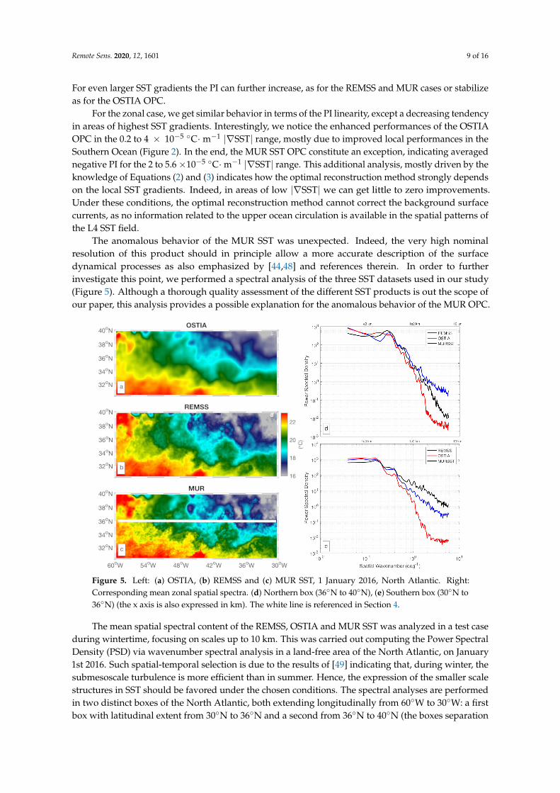
The anomalous behavior of the MUR SST was unexpected. Indeed, the very high nominalresolution of this product should in principle allow a more accurate description of the surfacedynamical processes as also emphasized by [44,48] and references therein. In order to furtherinvestigate this point, we performed a spectral analysis of the three SST datasets used in our study(Figure 5). Although a thorough quality assessment of the different SST products is out the scope ofour paper, this analysis provides a possible explanation for the anomalous behavior of the MUR OPC.

Figure 5. Left: (a) OSTIA, (b) REMSS and (c) MUR SST, 1 January 2016, North Atlantic. Right:Corresponding mean zonal spatial spectra. (d) Northern box (36◦N to 40◦N), (e) Southern box (30◦N to36◦N) (the x axis is also expressed in km). The white line is referenced in Section 4.

The mean spatial spectral content of the REMSS, OSTIA and MUR SST was analyzed in a test caseduring wintertime, focusing on scales up to 10 km. This was carried out computing the Power SpectralDensity (PSD) via wavenumber spectral analysis in a land-free area of the North Atlantic, on January1st 2016. Such spatial-temporal selection is due to the results of [49] indicating that, during winter, thesubmesoscale turbulence is more efficient than in summer. Hence, the expression of the smaller scalestructures in SST should be favored under the chosen conditions. The spectral analyses are performedin two distinct boxes of the North Atlantic, both extending longitudinally from 60◦W to 30◦W: a firstbox with latitudinal extent from 30◦N to 36◦N and a second from 36◦N to 40◦N (the boxes separation

Remote Sens. 2020, 12, 1601 10 of 16

is identified by the white line in Figure 5c). In both boxes, the baroclinic Rossby radius of deformationis around 30 km [50]. Investigating scales up to 10 km also enables to capture submesoscale features inthe area, whenever they are present.

In the southern box (30◦N to 36◦N, see also Figure 5e), the spectra of the REMSS, OSTIAand MUR SST are initially superimposed and so they evolve until scales of '200 km. Afterward,the OSTIA spectrum begins to separate, indicating a decreased amount of spatial variance at finer scales,eventually flattening around 50 km. On the other hand, the REMSS and MUR SST exhibit lager PSDthan the OSTIA SST, with a dominance of MUR until scales of 15 km, where REMSS is instead quite flat.If we consider the different nature of the three SST datasets described in Section 2, this is the expectedspectral behavior of the input SSTs for our application.

If the same spectral analysis is performed in the Northern box (Figure 5c,d), i.e., where theMUR SST looks smoother, the spectral properties of the MUR and REMSS SST are inverted. Indeed,the REMSS spectrum is characterized by larger PSDs at scales lower than 100 km. Therefore, theREMSS SSTs are associated with the finer effective spatial resolution in the Northern Area (36◦N to40◦N). This result is indicating that the global scale OPC based on MUR data can be negatively affectedby unequal effective SST resolutions in different areas of the ocean. Visual inspection of the MUR SSTfields evidenced that this non uniformity can happen throughout the year in different areas of theocean. This spectral inconsistency can have drawbacks on the computation of the SST spatio-temporalgradients, in which non physical dynamical structures can be recognized. An example is providedin Figure 6, showing |∇SST|maps on three different dates in the Gulf Stream, Kuroshio Current andAgulhas Current areas.

Figure 6. (a) |∇SST| in the Agulhas Current area; (b) same, in the Gulf Stream area; (c) same, in theKuroshio Current area. The images correspond to the |∇SST| based on MUR SST on three differentdates indicated in the panels.

Remote Sens. 2020, 12, 1601 11 of 16

On the other hand, the REMSS and OSTIA SSTs did not evidence non-homogeneities in theeffective resolution of the L4 fields, being coherent with the example provided in Figure 5 during theperiod 2014–2016.

However, selecting areas where the MUR SST are spatially uniform, this problem could beovercome and the fine resolution of the SST field can be fully exploited. In Figure 7, we perform aqualitative comparison between the MUR and REMSS OPC in the Agulhas Current. In the chosen area,the following three conditions are satisfied: (i) the SST spectra are comparable with the condition ofFigure 5e (not shown); (ii) according to Figures 1 and 3, both the components of MUR and REMSSOPC are improved based on a three-year statistic; (iii) the trajectory of a drifter in correspondence of aSST gradient was available (see also [33]).

Figure 7. Optimal current vectors (black arrows) based on the REMSS and MUR SST reconstruction.The SST field is given in colors. The trajectory of a drifter is given in white. The magenta and blackdots respectively stand for the buoy position from 25 March 2015 (00 UTC) to 26 March 2015 (00 UTC).The gridded fields represent 25 March 2015.

It is evident that the MUR SST describe a finer SST gradient than in the REMSS case. Moreover,the gridded current vectors provided by the MUR OPC exhibit a reduced angle with respect to thedrifter trajectory in the north-eastern section of the domain (where the drifter time is closer to the dateof the Eulerian fields, 25 March 2015).

Concluding, our study can be summarized by the following main items:

• The derivation of the sea surface currents from space can benefit from the synergy betweenoptimally interpolated space-based Earth observations from multiple platforms, today availableat an operational level and with nominal daily and global coverage. Based on recent works [33,47]we attempted to optimize the surface currents retrieval by combining the altimeter-derivedgeostrophic currents with satellite SST from Infrared (IR) and Microwave (MW) sensors. Our studywas based on three different L4 SST estimates: a dataset provided by Remote Sensing Systems,fully based on the optimal interpolation of satellite observations (IR and MW), and two additionaldatasets based on the optimal interpolation of satellite and in-situ data, i.e., the OSTIA andMUR SSTs.

• The REMSS and OSTIA OPC exhibited the best performances, with maximum overallimprovements equal to or larger than 15% with respect to the geostrophic estimates (for themeridional flow). This was achieved transferring the high resolution dynamical content of thesatellite-derived SST into the coarser resolution geostrophic current estimates [33,34]. However,the OSTIA OPC are characterized by larger improvements than the REMSS OPC in the 0.2 to4 ×10−5 ◦C·m−1 |∇SST| range. This result is due to enhanced performances of the OSTIA OPCin the 45◦S to 70◦S latitudinal band. This is illustrated by Figures 1, 2 and 4 and summarized byTable 1: the OSTIA OPC partially solve the degradation of the zonal flow in the Southern Ocean,also yielding slightly larger averaged PIs for the meridional flow.

Remote Sens. 2020, 12, 1601 12 of 16

Most likely, this is due to the larger number of sensors used to build the L4 SSTs as well as theuse of in-situ observations in the optimal interpolation procedure. This could optimize the SSTestimates at high latitudes, where cloud coverage is often very high and where average intensesurface winds degrade the satellite infrared and microwave SST retrievals [51,52]. An additionalanalysis is provided as Supplementary Materials (Figure S5).

However, despite the improved performances of the OSTIA OPC compared to the REMSS case,occasional degradations in the polar regions can also occur with the OSTIA SST, as shown inFigure 2. This emphasizes the importance of providing very high quality, high resolution andsynoptic SST measurements in those areas, highlighting the strong potential of future ESA satellitemissions like the Copernicus Imaging Microwave Radiometer (CIMR) [53] (https://cimr.eu).CIMR will provide global-scale, all-weather, 15 km effective spatial resolution SST observations,also guaranteeing sub-daily coverage at latitudes higher than±60◦. All the SST-based applicationswill benefit from the future CIMR remote sensing capabilities. Applying the RS18 method inhigh-latitude areas could also benefit from additional oceanic tracers as sea surface salinity.In polar areas, the contribution of salinity in determining the ocean dynamics can be relevant [54].

• The OPC based on the use of MUR very high resolution data, though showing degradedperformances at global scale, suggest that fine-scale SST gradients can be retrieved successfully.This is achieved when the MUR SST effective high resolution is homogenous in the study area,mostly indicating a potential for local applications.

Table 1. REMSS and OSTIA PI in the 45◦S to 70◦S latitudinal band. The results are given for the twoflow components.

45◦S–70◦S REMSS OSTIA

2SAT - ZONAL PI (%) −1.35 1.342SAT - MERIDIONAL PI (%) 5.60 6.434SAT - ZONAL PI (%) −2.48 0.104SAT - MERIDIONAL PI (%) 4.28 4.61

Therefore, in order to guarantee an accurate global OPC reconstructions via the methodof Piterbarg 2009 and RS18, the L4 SSTs have to contain the signature of fine scale SST gradients andguarantee spatial homogeneity of the optimally interpolated field. In this way, the zonal and meridionalSST gradients are not affected by the inhomogeneities like the ones reported in Figures 5 and 6.This work also identifies the RS18 method as a tool for indirect validation of the L4 SST products,allowing to test their dynamical content.

Supplementary Materials: The following figures are available online http://www.mdpi.com/2072-4292/12/10/1601/s1, Figure S1: Uncertainties on the zonal geostrophic currents (σu) and on the Forcing term (h) usedin Equation (5). Figure S2: Lagrangian buoy trajectories over the 2014–2016 period. Figure S3: Percentage ofimprovement of the Optimal Currents based on the MUR SST and the 4SAT geostrophic currents. Figure S4: Zonaland meridional percentages of improvement of the Optimal Currents based on the 4SAT geostrophic estimates(seen as a function of the local SST spatial gradients). Figure S5: Performances of the REMSS and OSTIA SSTevaluated via in-situ SST match-up analysis.

Author Contributions: Conceptualization, D.C., M.-H.R. and R.S.; methodology, D.C., M.-H.R. and R.S.; software,D.C., H.E. and M.-H.R.; validation, D.C., M.-H.R. and H.E..; formal analysis, D.C., H.E.; investigation, D.C.,M.-H.R., B.B.N., H.E. and R.S.; resources, R.S.; writing—original draft preparation, D.C.; writing—review andediting, B.B.N., M.-H.R., H.E.; visualization, D.C.; supervision, M.-H.R., B.B.N. and R.S.; funding acquisition, R.S.and B.B.N. All authors have read and agreed to the published version of the manuscript.

Funding: This work has been carried out as part of Copernicus Marine Environment Monitoring Service (CMEMS)Multi-Observation Thematic Assembly Centre (CMEMS-TAC-MOB), funded through Subcontracting Agreementn. CLS-SCO-18-0004 between Consiglio Nazionale delle Ricerche and Collecte Localisation Satellites (CLS), whichis presently leading the CMEMS-TAC-MOB. 83-CMEMS-TAC-MOB contract is funded by Mercator Ocean as partof its delegation agreement with the European Union, represented by the European Commission, to set-up andmanage CMEMS.

Remote Sens. 2020, 12, 1601 13 of 16

Acknowledgments: The Authors thank the three anonymous Reviewers for providing valuable comments toimprove the manuscript. D. Ciani acknowledges S. Marullo and A. Pisano for the discussions on the SST data.This paper also benefited from fruitful discussions with J. Vazquez-Cuervo, J. Gomez-Valdes, M.T. Chin and M.Bouali during the Ocean Sciences 2020 meeting in San Diego. Finally, the Authors thank the members of theRemote Sensing Editorial Office for taking care of the review process and publication of this manuscript.

Conflicts of Interest: The authors declare no conflict of interest. The funders had no role in the design of thestudy; in the collection, analyses, or interpretation of data; in the writing of the manuscript, or in the decision topublish the results.

Abbreviations

List of undefined abbreviations:

ADCP Acoustic Doppler Current ProfilerAMSR-E Advanced Microwave Scanning Radiometer - Earth Observing SystemAMSR-2 Second Advanced Microwave Scanning RadiometerAVHRR Advanced Very-High-Resolution RadiometerAVHRR-GAC Advanced Very-High-Resolution Radiometer - Global Area CoverageAVHRR-LAC Advanced Very-High-Resolution Radiometer - Local Area coverageCLS Collecte Localisation SatellitesDUACS Data Unification and Altimeter Combination SystemESA European Space AgencyHY2A Haiyang-2A satelliteMODIS Moderate-resolution Imaging SpectroradiometerNOAA AOML National Oceanic and Atmospheric Administration—Atlantic Oceanographic

and Meteorological LaboratorySVP Surface Velocity ProgramTMI Tropical Rainfall Measuring Mission Microwave ImagerL4 Level 4 processing analysisSSM/I Special Sensor Microwave/ImagerSSMIS Special Sensor Microwave Imager SounderVIIRS Visible Infrared Imaging Radiometer Suite (VIIRS)

References

1. Hátún, H.; Sandø, A.B.; Drange, H.; Hansen, B.; Valdimarsson, H. Influence of the Atlantic subpolar gyre onthe thermohaline circulation. Science 2005, 309, 1841–1844. [CrossRef] [PubMed]

2. Bashmachnikov, I.; Neves, F.; Calheiros, T.; Carton, X. Properties and pathways of Mediterranean watereddies in the Atlantic. Prog. Oceanogr. 2015, 137, 149–172. [CrossRef]

3. Buongiorno Nardelli, B. Vortex waves and vertical motion in a mesoscale cyclonic eddy. J. Geophys.Res. Ocean. 2013, 118, 5609–5624. [CrossRef]

4. Barbosa Aguiar, A.C.; Peliz, Á.; Carton, X. A census of Meddies in a long-term high-resolution simulation.Prog. Oceanogr. 2013, 116, 80–94. [CrossRef]

5. Ponte, A.; Klein, P.; Capet, X.; Le Traon, P.; Chapron, B.; Lherminier, P. Diagnosing surface mixedlayer dynamics from high-resolution satellite observations: Numerical insights. J. Phys. Oceanogr. 2013,43, 1345–1355. [CrossRef]

6. Frenger, I.; Gruber, N.; Knutti, R.; Munnich, M. Imprint of Southern Ocean eddies on winds,clouds and rainfall. Nat. Geosci. 2013, 6, 608–612. [CrossRef]

7. Chenillat, F.; Franks, P.J.; Combes, V. Biogeochemical properties of eddies in the California Current System.Geophys. Res. Lett. 2016, 43, 5812–5820. [CrossRef]

8. Siokou-Frangou, I.; Christaki, U.; Mazzocchi, M.G.; Montresor, M.; Ribera d’Alcalá, M.; Vaqué, D.; Zingone,A. Plankton in the open Mediterranean Sea: A review. Biogeosciences 2010, 7, 1543–1586. [CrossRef]

9. Olascoaga, M.J.; Beron-Vera, F.J.; Haller, G.; Trinanes, J.; Iskandarani, M.; Coelho, E.; Haus, B.K.; Huntley,H.; Jacobs, G.; Kirwan, A.; et al. Drifter motion in the Gulf of Mexico constrained by altimetric Lagrangiancoherent structures. Geophys. Res. Lett. 2013, 40, 6171–6175. [CrossRef]

Remote Sens. 2020, 12, 1601 14 of 16

10. Clarke, A.; Li, J. El Nino/La Nina shelf edge flow and Australian western rock lobsters. Geophys. Res. Lett.2004, 31. [CrossRef]

11. Li, J.; Clarke, A.J. Coastline direction, interannual flow, and the strong El Niño currents along Australia’snearly zonal southern coast. J. Phys. Oceanogr. 2004, 34, 2373–2381. [CrossRef]

12. Carlson, D.F.; Clarke, A.J. Seasonal along-isobath geostrophic flows on the west Florida shelf with applicationto Karenia brevis red tide blooms in Florida’s Big Bend. Cont. Shelf Res. 2009, 29, 445–455. [CrossRef]

13. Pisano, A.; De Dominicis, M.; Biamino, W.; Bignami, F.; Gherardi, S.; Colao, F.; Coppini, G.; Marullo, S.;Sprovieri, M.; Trivero, P.; et al. An oceanographic survey for oil spill monitoring and model forecastingvalidation using remote sensing and in situ data in the Mediterranean Sea. Deep Sea Res. Part II Top.Stud. Oceanogr. 2016, 133, 132–145. [CrossRef]

14. Onink, V.; Wichmann, D.; Delandmeter, P.; Van Sebille, E. The role of Ekman currents, geostrophy, and Stokesdrift in the accumulation of floating microplastic. J. Geophys. Res. Ocean. 2019, 124, 1474–1490. [CrossRef]

15. Cazenave, A.; Palanisamy, H.; Ablain, M. Contemporary sea level changes from satellite altimetry: Whathave we learned? What are the new challenges? Adv. Space Res. 2018, 62, 1639–1653. [CrossRef]

16. Vallis, G.K. Atmospheric and Oceanic Fluid Dynamics; Cambridge University Press: Cambridge, UK, 2006;p. 745.

17. Pujol, M.I.; Dibarboure, G.; Le Traon, P.Y.; Klein, P. Using high-resolution altimetry to observemesoscale signals. J. Atmos. Ocean. Technol. 2012, 29, 1409–1416. [CrossRef]

18. Pujol, M.I.; Faugère, Y.; Taburet, G.; Dupuy, S.; Pelloquin, C.; Ablain, M.; Picot, N. DUACS DT2014: The newmulti-mission altimeter data set reprocessed over 20 years. Ocean. Sci. 2016, 12, 1067–1090. [CrossRef]

19. Ballarotta, M.; Ubelmann, C.; Pujol, M.I.; Taburet, G.; Fournier, F.; Legeais, J.F.; Faugère, Y.; Delepoulle,A.; Chelton, D.; Dibarboure, G.; et al. On the resolutions of ocean altimetry maps. Ocean. Sci. 2019,15, 1091–1109. [CrossRef]

20. Chapron, B.; Collard, F.; Ardhuin, F. Direct measurements of ocean surface velocity from space: Interpretationand validation. J. Geophys. Res. Ocean. 2005, 110. [CrossRef]

21. Poulain, P.M. Adriatic Sea surface circulation as derived from drifter data between 1990 and 1999. J. Mar. Syst.2001, 29, 3–32. [CrossRef]

22. Falco, P.; Zambianchi, E. Near-surface structure of the Antarctic Circumpolar Current derived from WorldOcean Circulation Experiment drifter data. J. Geophys. Res. Ocean. 2011, 116, C05003. [CrossRef]

23. Lumpkin, R.; Özgökmen, T.; Centurioni, L. Advances in the application of surface drifters. Annu. Rev.Mar. Sci. 2017, 9, 59–81. [CrossRef] [PubMed]

24. Laurindo, L.C.; Mariano, A.J.; Lumpkin, R. An improved near-surface velocity climatology for the globalocean from drifter observations. Deep Sea Res. Part I Oceanogr. Res. Pap. 2017, 124, 73–92. [CrossRef]

25. Capodici, F.; Cosoli, S.; Ciraolo, G.; Nasello, C.; Maltese, A.; Poulain, P.M.; Drago, A.; Azzopardi, J.; Gauci,A. Validation of HF radar sea surface currents in the Malta-Sicily Channel. Remote Sens. Environ. 2019,225, 65–76. [CrossRef]

26. Berta, M.; Griffa, A.; Magaldi, M.G.; Özgökmen, T.M.; Poje, A.C.; Haza, A.C.; Olascoaga, M.J. Improvedsurface velocity and trajectory estimates in the Gulf of Mexico from blended satellite altimetry and drifterdata. J. Atmos. Ocean. Technol. 2015, 32, 1880–1901. [CrossRef]

27. Mulet, S.; Etienne, H.; Ballarotta, M.; Faugere, Y.; Rio, M.; Dibarboure, G.; Picot, N. Synergy between surfacedrifters and altimetry to increase the accuracy of sea level anomaly and geostrophic current maps in the Gulfof Mexico. Adv. Space Res. 2020. [CrossRef]

28. Isern-Fontanet, J.; Chapron, B.; Lapeyre, G.; Klein, P. Potential use of microwave sea surface temperaturesfor the estimation of ocean currents. Geophys. Res. Lett. 2006, 33. [CrossRef]

29. González-Haro, C.; Isern-Fontanet, J. Global ocean current reconstruction from altimetric and microwaveSST measurements. J. Geophys. Res. Ocean. 2014, 119, 3378–3391. [CrossRef]

30. Bowen, M.M.; Emery, W.J.; Wilkin, J.L.; Tildesley, P.C.; Barton, I.J.; Knewtson, R. Extracting multiyear surfacecurrents from sequential thermal imagery using the maximum cross-correlation technique. J. Atmos. Ocean.Technol. 2002, 19, 1665–1676. [CrossRef]

31. Qazi, W.A.; Emery, W.J.; Fox-Kemper, B. Computing ocean surface currents over the coastal California currentsystem using 30-min-lag sequential SAR images. IEEE Trans. Geosci. Remote. Sens. 2014, 52, 7559–7580.[CrossRef]

Remote Sens. 2020, 12, 1601 15 of 16

32. Warren, M.; Quartly, G.; Shutler, J.; Miller, P.; Yoshikawa, Y. Estimation of ocean surface currents frommaximum cross correlation applied to GOCI geostationary satellite remote sensing data over the Tsushima(Korea) Straits. J. Geophys. Res. Ocean. 2016, 121, 6993–7009. [CrossRef]

33. Rio, M.H.; Santoleri, R. Improved global surface currents from the merging of altimetry and Sea SurfaceTemperature data. Remote Sens. Environ. 2018, 216, 770–785. [CrossRef]

34. Piterbarg, L.I. A simple method for computing velocities from tracer observations and a model output. Appl.Math. Model. 2009, 33, 3693–3704. [CrossRef]

35. Mercatini, A.; Griffa, A.; Piterbarg, L.; Zambianchi, E.; Magaldi, M.G. Estimating surface velocities fromsatellite data and numerical models: Implementation and testing of a new simple method. Ocean. Model.2010, 33, 190–203. [CrossRef]

36. Taburet, G.; Sanchez-Roman, A.; Ballarotta, M.; Pujol, M.I.; Legeais, J.F.; Fournier, F.; Faugere, Y.;Dibarboure, G. DUACS DT2018: 25 years of reprocessed sea level altimetry products. Ocean Sci. 2019,15, 1207–1224. [CrossRef]

37. Pascual, A.; Faugère, Y.; Larnicol, G.; Le Traon, P.Y. Improved description of the ocean mesoscale variabilityby combining four satellite altimeters. Geophys. Res. Lett. 2006, 33. [CrossRef]

38. Gentemann, C.L.; Donlon, C.J.; Stuart-Menteth, A.; Wentz, F.J. Diurnal signals in satellite sea surfacetemperature measurements. Geophys. Res. Lett. 2003, 30. [CrossRef]

39. Martin, M.; Dash, P.; Ignatov, A.; Banzon, V.; Beggs, H.; Brasnett, B.; Cayula, J.F.; Cummings, J.; Donlon, C.;Gentemann, C.; et al. Group for High Resolution Sea Surface temperature (GHRSST) analysis fieldsinter-comparisons. Part 1: A GHRSST multi-product ensemble (GMPE). Deep Sea Res. Part II Top.Stud. Oceanogr. 2012, 77, 21–30. [CrossRef]

40. Gentemann, C.L.; Meissner, T.; Wentz, F.J. Accuracy of satellite sea surface temperatures at 7 and 11 GHz.IEEE Trans. Geosci. Remote. Sens. 2009, 48, 1009–1018. [CrossRef]

41. Donlon, C.J.; Martin, M.; Stark, J.; Roberts-Jones, J.; Fiedler, E.; Wimmer, W. The operational sea surfacetemperature and sea ice analysis (OSTIA) system. Remote Sens. Environ. 2012, 116, 140–158. [CrossRef]

42. Good, S.; Fiedler, E.; Mao, C.; Martin, M.J.; Maycock, A.; Reid, R.; Roberts-Jones, J.; Searle, T.; Waters, J.;While, J.; et al. The Current Configuration of the OSTIA System for Operational Production of FoundationSea Surface Temperature and Ice Concentration Analyses. Remote. Sens. 2020, 12, 720. [CrossRef]

43. Martin, M.; Hines, A.; Bell, M. Data assimilation in the FOAM operational short-range oceanforecasting system: A description of the scheme and its impact. Q. J. R. Meteorol. Soc. 2007, 133, 981–995.[CrossRef]

44. Chin, T.M.; Vazquez-Cuervo, J.; Armstrong, E.M. A multi-scale high-resolution analysis of global seasurface temperature. Remote. Sens. Environ. 2017, 200, 154–169. [CrossRef]

45. Lumpkin, R.; Grodsky, S.A.; Centurioni, L.; Rio, M.H.; Carton, J.A.; Lee, D. Removing spurious low-frequencyvariability in drifter velocities. J. Atmos. Ocean. Technol. 2013, 30, 353–360. [CrossRef]

46. Rio, M.H.; Santoleri, R.; Bourdalle-Badie, R.; Griffa, A.; Piterbarg, L.; Taburet, G. Improving theAltimeter-Derived Surface Currents Using High-Resolution Sea Surface Temperature Data: A FeasabilityStudy Based on Model Outputs. J. Atmos. Ocean. Technol. 2016, 33, 2769–2784. [CrossRef]

47. Ciani, D.; Rio, M.H.; Menna, M.; Santoleri, R. A Synergetic Approach for the Space-Based Sea SurfaceCurrents Retrieval in the Mediterranean Sea. Remote. Sens. 2019, 11, 1285. [CrossRef]

48. Vazquez-Cuervo, J.; Gomez-Valdes, J.; Bouali, M.; Miranda, L.E.; Van der Stocken, T.; Tang, W.; Gentemann, C.Using saildrones to validate satellite-derived sea surface salinity and sea surface temperature along theCalifornia/Baja Coast. Remote. Sens. 2019, 11, 1964. [CrossRef]

49. Callies, J.; Ferrari, R.; Klymak, J.M.; Gula, J. Seasonality in submesoscale turbulence. Nat. Commun. 2015,6, 6862. [CrossRef]

50. Chelton, D.; De Szoeke, R.; Schlax, M.; El Naggar, K.; Siwertz, N. Geographical Variability of the FirstBaroclinic Rossby Radius of Deformation. J. Phys. Oceanogr. 1998, 28, 433–459. [CrossRef]

51. González-Haro, C.; Autret, A.P. Quantifying Tidal Fluctuations in Remote Sensing Infrared SST Observations.Remote. Sens. 2019, 11, 2313. [CrossRef]

52. Wentz, F.; Meissner, T.; Gentemann, C.; Hilburn, K.; Scott, J. Remote Sensing Systems GCOM-W1 AMSR2Daily Data, Environmental Suite on 0.25 Degrees Grid, 2014, Version V.8. Available online: www.remss.com/missions/amsr (accessed on 1 February 2020).

Remote Sens. 2020, 12, 1601 16 of 16

53. Donlon, C.J. Copernicus Imaging Microwave Radiometer (CIMR) Mission Requirements Document; Version 3.0;European Space Agency: Noordwijk, The Netherlands, 2019.

54. Roquet, F.; Madec, G.; Brodeau, L.; Nycander, J. Defining a simplified yet realistic equation of statefor seawater. J. Phys. Ocean. 2015, 45, 2564–2579. [CrossRef]

c© 2020 by the authors. Licensee MDPI, Basel, Switzerland. This article is an open accessarticle distributed under the terms and conditions of the Creative Commons Attribution(CC BY) license (http://creativecommons.org/licenses/by/4.0/).