Improving the consistency of particle size measurement€¦ · · 2017-08-01Good Practice Guide...

A NATIONAL MEASUREMENT

GOOD PRACTICE GUIDE

No. 111

Improving the consistency of particlesize measurement

A NATIONAL MEASUREMENT

GOOD PRACTICE GUIDE

No. 111

Improving the consistency of particlesize measurement

Measurement Good Practice Guide No. 111

Good Practice Guide for Improving the Consistency of Particle Size Measurement

K Mingard*, R Morrell*, P Jackson+, S Lawson†, S Patel† and R Buxton‡

*Industry and Innovation of Division, National Physical Laboratory +CERAM Research

†Particles CIC, University of Leeds ‡Particle Technology Ltd

ABSTRACT The principal causes of variability in particle size measurement, particularly in the sub-sieve range of 50 µm to sub 1 µm are summarised. The causes are illustrated with results of measurements from a series of round robins made to test reproducibility under different levels of prescription in the procedure followed. Improvements of over 50% in coefficient of variability for particle size fractions are shown to be possible when clear procedures are laid down for sampling, dispersion and handling even where different equipment constrains the exact procedure adopted. Users are encouraged to develop clear procedures based on the major factors described in the guide for each different powder encountered.

© Crown copyright 2009 Reproduced with the permission of the Controller of HMSO

and the Queen's Printer for Scotland

ISSN 1368-6550

National Physical Laboratory Hampton Road, Teddington, Middlesex, TW11 0LW

Extracts from this report may be reproduced provided the source is acknowledged and the extract is not taken out of context.

Approved on behalf of the Managing Director, NPL by Dr M G Cain, Knowledge Leader,

Industry and Innovation Division Acknowledgements This guide has been produced in a Processing of Advanced Materials project, part of the Materials Measurement programme sponsored by the National Measurement System unit of the UK’s Department for Innovation Universities and Skills. The advice and steer from the members of the PowdermatriX Knowledge Transfer Network and numerous practitioners of particle size measurement are gratefully acknowledged. For further information on Materials Measurement contact the Materials Enquiry Point at the National Physical Laboratory: Tel: 020 8943 6701 Fax: 020 8943 7160 E-mail: [email protected]

Good Practice Guide 111

Good Practice Guide for Improving the Consistency of Particle Size Measurement Contents

1 Executive Summary ......................................................... 1

2 Introduction .................................................................. 3 1.1 Objectives ..................................................................................................................4 1.2 Background................................................................................................................4 1.3 Scope..........................................................................................................................5

3 Definitions and particle sizing terminology ............................ 7 2.1 Definitions..................................................................................................................8 2.2 Reporting of particle size .........................................................................................10

2.2.1 Definition of particle size.................................................................................10 2.2.2 Particle size distributions .................................................................................11

4 Measurement Principles...................................................13 3.1 Measurement Methods.............................................................................................14 3.2 Laser diffraction.......................................................................................................15 3.3 Sedimentation methods............................................................................................16 3.4 Electrozone sensing .................................................................................................17

5 Performing a Measurement ...............................................18 4.1 Sampling and sub-sampling.....................................................................................19 4.2 Powder dispersion....................................................................................................21

4.2.1 Creating a suspension ......................................................................................21 4.2.2 Control of solid-liquid interactions..................................................................23 4.2.3 Maintaining a dispersion in the measurement system .....................................25 4.2.4 Effect of density...............................................................................................25

4.3 Measurement............................................................................................................26 4.3.1 Use of ultrasonics to control dispersion in liquids...........................................26 4.3.2 Particle concentration.......................................................................................27 4.3.3 Measurement time & number of measurements ..............................................29 4.3.4 Optical model...................................................................................................30 4.3.5 Refractive index ...............................................................................................31 4.3.6 Electrozone sensing .........................................................................................34 4.3.7 Optical examination for confirmation..............................................................35

6 Variability of Results: Outcome of Round Robin Studies............36 5.1 Introduction..............................................................................................................37 5.2 Round robin structure ..............................................................................................37 5.3 Comparison of starting and final round robins ........................................................37

7 Recommendations ..........................................................42 6.1 Sources of information.............................................................................................43

6.1.1 Standards..........................................................................................................43 6.1.2 Manufacturers ..................................................................................................43

Measurement Good Practice Guide No 111

6.1.3 Training............................................................................................................43 6.2 Reference powders...................................................................................................44 6.3 Major practical issues for laser diffraction ..............................................................45

6.3.1 Sampling ..........................................................................................................45 6.3.2 Initial dispersion of sample..............................................................................45 6.3.3 Maintaining a stable dispersion .......................................................................45 6.3.4 Refractive Indices ............................................................................................45

8 Appendix 1...................................................................46 Appendix 1: A simple checklist for particle size measurement...........................................47

9 Appendix 2...................................................................53 Appendix 2: Sources of information on particle size measurement ...................................54

10 Appendix 3 .................................................................55 Appendix 3: Listing of standard test methods for particle size measurement .....................56 ISO Standards ......................................................................................................................56 Addresses of standards organisations ..................................................................................57

11 Appendix 4 .................................................................58 Appendix 4: Powder Sampling ............................................................................................59

12 Appendix 5 .................................................................62 Appendix 5: Round Robin Data Sheets ...............................................................................63


1

1Executive Summary IN THIS CHAPTER

Executive Summary


2

Executive Summary Particle size measurement has a reputation for lacking repeatability between laboratories, and of being subject to wide variations of practice despite efforts made by instrument suppliers to provide training and support. Measurements made at different laboratories, even using identical analytical apparatus, are prone to significant variations. This can lead to disputes between powder suppliers and users as to whether a batch of material is fit for purpose. Delays in delivery, reductions in processing rates / yield and increased waste etc. can then impact negatively on profitability along the supply chain. Recognising the importance of improving upon this situation NPL, in collaboration with CERAM Research, Particles CIC (University of Leeds) and Particle Technology Ltd, underpinned by the Knowledge Transfer Network node PowdermatriX and with financial support of the UK Department for Innovation, Universities and Skills (DIUS), set about improving understanding of the problems and investigating test repeatability. This Guide has been prepared with the objective of providing a concise overview of some of the key issues involved in making particle size measurements, particularly in the sub-sieve range of 50 µm to <1 µm, which encompasses a major fraction of the powder trade. It is not the intention of this guide to replace equipment manufacturers’ manuals, training courses, national and international measurement standards or textbooks, but to supplement them with recommendations based on the studies that have been made by the project partners and by findings from a series of wide round robins made to test the reproducibility under different levels of prescription of procedure. In creating such a guide the emphasis is very much to avoid labelling a given approach as “right” or “wrong” but rather to alert users to the impact of the approach they choose. Most importantly, the guide encourages users to make firm decisions on the approach they will use at each stage and to stick to that approach as “their protocol”. The round robin testing was intended to identify and demonstrate the most important variables involved in poor reproducibility. ‘Industrial’ powders (SiO2, CaCO3, Ni and WC) were selected, and both core and industrial partners carried out a range of measurements. In Phase 1, partners were given carte blanche in making measurements but encouraged to list exactly how measurements were made. In Phase 2 participants were given clear instructions on how to make measurements. Conclusions from an analysis of the returned data are incorporated into the recommendations. In addition, core partners undertook work in which (a) poor practice was deliberately used, and (b) technicians from one centre attempted to carry out measurements at another centre with laser diffraction apparatus that was not familiar to them. The above all helped to tease out the factors having the greatest influence on results. Key sources of problems that have been demonstrated include sampling procedures, methods for the initial dispersion of the sample, maintenance of a stable dispersion, and when using optical diffraction methods, employing the correct refractive index data for use of Mie scattering theory.


3

2Introduction IN THIS CHAPTER

11

Objectives

Background


4

1 Introduction 1.1 Objectives The driving force behind the production of this Guide came from the many reports and requests by members of Powdermatrix1 (a node within the Materials Knowledge Transfer Network), for a better understanding of the reasons behind the variability of particle size data. Whilst both customers and suppliers of powders desire tight specifications to control product quality, such specifications are difficult to draw up or to adhere to if the measured values vary significantly with operator, procedure and equipment, even where the equipment uses the same basic principle of measurement. The variability and a lack of understanding of this variability was reported to be worst for powder samples with sizes (or a substantial fraction of these sizes) too small to be easily measured by a sieve technique, which is generally taken to be about 50 μm. This represents a major fraction of trade in powders. This Guide therefore seeks to summarise the information and advice relevant to reducing variability from particle size measurement, supported by data derived from a series of round robin studies on a range of industrially used powders carried out in conjunction with writing this guide.

1.2 Background Typically 70% of all solid materials are particulate in nature at some stage of their processing. Almost all powders exhibit a spread of particles distributed over a range of sizes, and the width, shape and position of this distribution will influence all aspects of their processing. For example, powder handling characteristics will be influenced by changes to flow properties or a tendency to segregate – both phenomena correlating strongly with changes in the powder size distribution. Knowledge of particle size and the distribution of sizes are therefore essential for tight process control, maintenance of quality and minimisation of costs. Accurate and reproducible measurement techniques/protocols are required which in turn requires a clear definition of the particle size being measured. Some of the key issues are:

o That particle size can be defined by many different parameters which, except for the rare occurrence of spherical particles, are not simply related to one another.

o Distributions of sizes can be reported in terms of number, length, surface area or

volume with the inter-relationships between them also dependent on the particle shape.

o A number of different measurement techniques exist, but because they use different

physical effects to produce the size parameters, even for identical samples of an homogeneous powder, a range of results should be expected from the different techniques and there is no simple conversion between the different parameters used.

1 www.powdermatrix.org


5

o The statistical nature of powders also means that there will always be some

variability between samples taken from an homogeneous batch unless an infinitely large sample is taken, whilst in practice this is generally much smaller than the variability introduced by the method of dispersing and presenting the powder in the equipment used.

With modern equipment, routine measurement of samples from powders of a known and regularly measured type can be highly reproducible when undertaken by trained operators using a defined set procedure on a set item of equipment. Individual companies often have standard operating procedures (SOPs) for measurement of particle size, but a procedure for measuring one particular material is not necessarily suitable for measuring another type. While equipment manufacturers offer excellent training in how to optimise techniques for different samples, this general training is often not passed on to new operators of existing, rather than new, equipment. Thus it is often the case that when a powder sample has to be measured with different equipment, different companies or by operators perhaps relatively unfamiliar with the powder properties, wide variation in particle size distributions are obtained. 1.3 Scope Defining a single correct way to carry out particle size characterisation is not possible, so this Guide will aim to emphasise the key factors that have a strong potential to cause variation in results and then to encourage suppliers and users to define their own measurement protocols. This guide cannot be exhaustive but aims to quickly focus the mind of users on the issues that dominate in particle size measurement variability. A simple table/check list is provided in Appendix 1 to assist personnel responsible for particle size measurement to quickly develop suitable protocols. A number of excellent readily available sources of information on particle size measurement techniques have already been published (see Appendix 2) and will be referred to throughout the report. However, this information is lengthy and so runs the risk of being overlooked or not frequently referenced by industrial staff under great pressure to manage and make numerous particle size measurements to a demanding time-scale. This Guide will firstly then, attempt to summarise the information and advice relevant to reducing variability that can be found from sources such as International Standards, equipment manufacturers and from the scientific literature. Secondly it will illustrate the most frequent sources of variability with examples derived from round robin studies carried out in conjunction with writing this report. These round robins provided an overview and more importantly quantification of the typical level of variability that may be expected from different laboratories when measuring relatively unknown powders. The round robin studies were structured to illustrate what can be expected in terms of spread results from a range of standard practices currently in use (Phase 1) and what improvements can be delivered if a common closely defined procedure is followed (Phase 2). A summary of these round robins is given in Section 6 of this guide, but the results from the full range of powder types and sizes covered by the round robins will be given in a separate report 2.

2 NPL Report “Final Report on Powder Sizing Round Robins”, to be published


6

Preparation and analysis of the powders used in the round robin was carried out by three companies actively involved in the measurement and use of particle size data:

o CERAM Research, o ParticlesCIC, University of Leeds o Particle Technology Ltd.

These companies also carried out additional testing to explore effects of deliberately varying measurement practices on the variability of the powders used in the round robins, and the results of this testing are incorporated in this Guide.


7

3Definitions and particle sizing terminology

IN THIS CHAPTER

22

Terminology

Reporting Particle Size and Distributions


8

2 Definitions and particle sizing terminology 2.1 Definitions Aliquot A fraction of a dispersed sample used for analysis Batch A consignment of powder, nominally of consistent character Coefficient of variation Relative measure (%) for precision: standard deviation divided by mean value of population and multiplied by 100 (only for normal distributions of data is the median is equal to the mean) Cumulative oversized distribution plot A graph which plots, against the particle size (x axis), the fraction of particles greater than that particle size (y axis). Cumulative undersized distribution plot A graph which plots, against the particle size (x axis), the fraction of particles smaller than that particle size (y axis). Diameter A single dimension describing the size of a particle which may be a true spherical diameter but generally for irregular particles will be the diameter of a sphere having equivalent properties (e.g. area or volume) to that of the particle (see section 2.2). The standard ISO 9276-1 uses the symbol x but states that the symbol d may also be used. In practice, particle size data is described most commonly using d rather than x, and this convention will be used throughout this guide. d10, d50, d90 (sometimes d(v0.1), d(v0.5), d(v0.9)) A particle size value indicating that, respectively, 10%, 50% and 90% of the distribution is below this value, i.e. a d10 of 1.23µm means 10% of the sample is below 1.23µm in size (using a volume based calculation). d(3,2) Surface area mean diameter or Sauter mean diameter. It is the weighted average surface diameter, assuming spherical particles of the same surface area as the actual particles (see section 2.2.2).


9

d(4,3) The volume mean diameter or de Brouckere mean diameter. It is the weighted average volume diameter, assuming spherical particles of the same volume as the actual particles (see section 2.2.2). Dispersant A fluid medium that does not alter any characteristics of the particulates but enables the separation of the sample down to the primary particles Dispersion / suspension The separation of particles into a fluid (liquid or gas) for the purposes of treating them as separate entities Fraunhofer theory The optical theory that can be derived from the Mie theory or based on diffraction of light from particles, applicable to particles that are large compared to the wavelength of the incident light, which enables particle size to be derived from the diffraction pattern. Mie scattering The theory that describes the scattering of light by spherical particles. The real and imaginary indices of light refraction of the particles are needed, but the theory can be applied to particles smaller than the wavelength of the incident light. Multiple scattering Scattering of light during laser diffraction measurements by more than one particle, causing a scattering pattern that is no longer the sum of the patterns from all individual particles (in contrast to single scattering). Obscuration In optical methods, the optical concentration, percentage or fraction of incident light that is attenuated due to extinction (scattering and/or absorption) by the particles. [ISO Standard 13320-1] Particle A discrete element of material regardless of its size [ISO Standard 13320-1] Powder A dry collection of particulates with a macroscopic consistency. [ISO Standard 13320-1]


10

Reynolds number The dimensionless number which defines the flow pattern of a fluid surrounding a particle. Sample A portion of material intended to be representative of the whole Stokes diameter Equivalent spherical diameter of the particle that has the same density and terminal settling velocity as the real particle in the same liquid under creeping flow conditions [ISO13317-1] Stokes law The equation from which particle size can be calculated using the free-falling velocity measured for particles falling under viscous flow conditions. Sub-sample A fraction of a sample selected for a single measurement. 2.2 Reporting of particle size 2.2.1 Definition of particle size Particle size and particle size distribution are usually reported in terms of diameter irrespective of the actual particle shape; commonly this diameter is the equivalent sphere diameter, defined by ISO 9276-1 as the diameter of a sphere having the same physical attributes as the particle. In many cases the equivalent sphere is one with the same volume as the particle, but the method of measurement and the property of interest in the powder can lead to the use of other diameters defined by, for example, the surface area, or based on a statistical measurement such as the Feret diameters measured by image analysis. A detailed list of the possible options for description of particle diameters is given in the Recommended Practice Guide 960 published by NIST3. Clearly, irregularly shaped particles can lead to very different diameter measurements depending on the definition chosen. This range of possible descriptions of size gives one indication that different techniques or even different equipment using the same basic technique are likely to produce different size measurements from the same powder sample. Different methods, even different equipment suppliers employing the same basic method, will use different algorithms to convert the effect of an irregularly shaped particle (e.g. on rate of sedimentation or scattering of light) into the equivalent effect that would be produced by an idealised sphere. The effects of the approximations that these algorithms use often become more pronounced at the extremes of a distribution and thus can have a significant effect on values calculated to describe the distribution.

3 Ajit Jillavenkatesa, Stanley J. Dapkunas, Lin-Sien H. Lum, Particle size characterization, NIST Special publication 960-1, downloadable from the NIST website: http://www.msel.nist.gov/practiceguides/SP960_1.pdf


11

Analysis by laser diffraction is measured in volume, with transformations to number, length and area possible. However caution should be taken as the errors associated with the analysis are cubed through the transformation. The chance of incurring errors is increased in the sub micron region and can be greater than 15%. If a distribution is whole, i.e. there is no missing component then the errors associated with the transformation are minimised. If there is a portion missing then the errors are significant and the transformation should not be relied upon. In the schematic Figure 2.1 below distribution A is suitable for transformation whilst distribution B has been truncated (e.g. because below the lower limit of measurement) and therefore there is no data for small particles to include in a transformation.

A

B

Figure 2.1: Schematic showing a truncated distribution B which is not suitable for conversion between volume and, for example, area distributions, compared with the narrower but more complete distribution A, which could be converted. (Adapted from Malvern Instruments Ltd diagram). 2.2.2 Particle size distributions The distribution can be reported in graphical format, or for the purposes of specifications and quality control measurements more commonly as one or more diameters that describe the size at particular fractions or statistical descriptions of the distribution. Graphically the distribution may be shown either as a density (or differential) distribution or as a cumulative plot, generally with increasing particle diameter. Each type has its own advantages. The density distribution presents a clear description of the distribution spread and the peak (mode) and whether the peak is skewed from the centre of the distribution. It will also show if the distribution is multi-modal with more than one peak. In a cumulative plot small multi-modal peaks may not be easily observed, but this form of graphical output enables simple identification of the fractional distribution of sizes dnn where the subscript ‘nn’ is the percentage (by volume, area, etc. depending on the definition of d) of particles with dimensions less than d. The values most frequently measured in this form are d10, d50, and d90 which give an indication of size of the fine (d10) and coarse (d90) fractions, and of the median particle size (d50). While the median particle size indicates the centre of the size distribution, this is unlikely to be the same as the mean particle size. The mean particle size can be defined in many ways;


12

ISO 9276-2 describes methods for calculating this, but many other texts give good descriptions of their derivation4,5. Number means are familiar to most users, being given simply by the sum of the diameters (or cube root of the sum of the diameters cubed, if volume is considered) divided by the number of particles. This has however a number of disadvantages including the need to count a large number of particles, and the way in which a large number of very small particles can weight the result even though they comprise a very small proportion of the total volume. Because of these disadvantages, ‘moment means’ are frequently quoted, and in this Guide the de Brouckere mean or volume (equivalent to mass, for a fixed density) moment mean is used, analogous to the centre of gravity of the distribution. Generally this mean is shown by the subscripts ‘4,3’, so using the terminology described earlier, this mean would be shown by x4,3 or d4,3. Calculations of moment means are given in the standard ISO 9276-2, although confusingly here the notation used gives this mean as 3,1x . Other derivations maybe found elsewhere5, which show the calculation simply as:

∑∑= 3

4

3,4d

dd

4 Introduction to Particle Technology, ed. Martin Rhodes, J.Wiley, 2008. ISBN 04700 14288 5 http://www.malvern.com/malvern/kbase.nsf/0/5E3F5A148D336B0480256BF2006E2195/$file/ Basic_principles_of_particle_size_analysis_MRK034-low_res.pdf 5 http://www.malvern.com/malvern/kbase.nsf/0/5E3F5A148D336B0480256BF2006E2195/$file/ Basic_principles_of_particle_size_analysis_MRK034-low_res.pdf


13

4Measurement Principles

IN THIS CHAPTER

33

Summary of Methods of Measurement

o Laser Diffraction

o Sedimentation

o Electrozone Sensing


14

3 Measurement Principles 3.1 Measurement Methods There is a wide range of measurement methods for particle sizing, each of which has capability over a certain range of particle size. Figure 3.1 provides a guide to the particle size ranges that are said to be measurable by each technique. For particles greater than about 50 µm in diameter, the simplest method is probably sieving. This in effect provides a go/no-go test for particle size. For particles less than 100 µm, the focus of this Guide, usually indirect measurement methods are employed. The principal methods that have been studied in the course of preparing this Guide are the following:

o Laser diffraction o Sedimentation of a suspension o Electrozone sensing

Other techniques are feasible, such image analysis, but these have not been examined in detail. Since Laser Diffraction was the technique of choice for the vast majority of industrial companies taking part in Round Robin work, findings and recommendations inevitably and unavoidably lean towards this technique. However, users of other techniques should find plenty of useful prompts.

0.00001 0.0001 0.001 0.01 0.1 1 10 100 1000

Automatic image analysis (electron microscope images)

Centrifugal sedimentation

Laser diffraction

Coulter counter

Gravimetric sedimentation

Photo-optical methods

Ultrasonic sieving

Air jet sieving

Wet sieving with test sieves

Optical image analysis

Dry sieving with test sieves

Sieving/visual check with pinhole template

0.00001 0.001

0.00001 0.01

0.00002 0.5

0.0005 0.3

0.001 0.25

0.001 3

0.005 0.1

0.02 0.2

0.02 3

0.03 30

0.03 125

Particle size [mm]

0.00001 0.0001 0.001 0.01 0.1 1 10 100 1000



Laser diffraction

Coulter counter



Ultrasonic sieving

Air jet sieving





0.00001 0.001

0.00001 0.01

0.00002 0.5

0.0005 0.3

0.001 0.25

0.001 3

0.005 0.1

0.02 0.2

0.02 3

0.03 30

0.03 125

Particle size [mm]



Laser diffraction

Coulter counter



Ultrasonic sieving

Air jet sieving





0.00001 0.001

0.00001 0.01

0.00002 0.5

0.0005 0.3

0.001 0.25

0.001 3

0.005 0.1

0.02 0.2

0.02 3

0.03 30

0.03 125

Particle size [mm] Figure 3.1: Schematic diagram of the particle size ranges in which each sizing method is thought to be capable of operating. (After: Retsch GmbH 6 ) 6 http://www.retsch.com/dltmp/www/5930-dd2ab7d5b08f/af_sieving%20basics_2004_en.pdf


15

3.2 Laser diffraction The principles of laser diffraction for particle sizing are comprehensively summarised in the international standard ISO/DIS 13320 and the NIST Recommended Practice Guide 960-1 3. Laser light incident on a particle is diffracted by interaction with the particle surface, producing a pattern of light intensity which can be captured by multi-element detectors around the beam and particle. All other parameters being constant, the pattern is characteristic of the particle size and, using either the Mie or Fraunhofer theories, deconvolution of the pattern yields a volumetric particle size distribution. The general assumption in laser diffraction is that particles are spherical; calculations within the software work out an equivalent sphere based on particle volume. Particles that deviate from a sphere such as needles and platelets (chalk, clays and crystalline materials) produce a reduction in the accuracy of the reported sizes (a single size might in fact be considered insufficient to describe such particles accurately). This is due to the 2-dimensional features of the platelets and needles. For instance the following figure demonstrates the range of shapes for calcium carbonate. The calculations will not be accurate either if light is scattered by more than one particle, so there is a clear requirement that the concentration of particles passing through the system is controlled below a certain limit.

Figure 3.2: Images of individual particles of calcium carbonate (from a Malvern Sysmex instrument). Both theories can be applied to particles larger than the laser light wavelength, but only the Mie theory can be applied to particles smaller than this limit. It relies on knowing both the real and imaginary parts of the particle’s refractive index, which, while generally well defined and documented for the real component of most materials is much harder to obtain/determine for the imaginary component as it depends on the shape and surface

3 See p.6


16

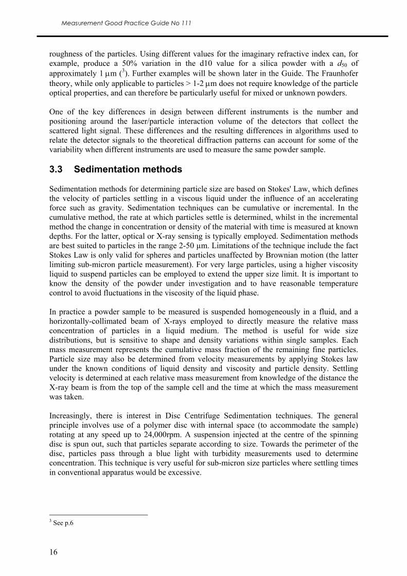
roughness of the particles. Using different values for the imaginary refractive index can, for example, produce a 50% variation in the d10 value for a silica powder with a d50 of approximately 1 μm (3). Further examples will be shown later in the Guide. The Fraunhofer theory, while only applicable to particles > 1-2 μm does not require knowledge of the particle optical properties, and can therefore be particularly useful for mixed or unknown powders. One of the key differences in design between different instruments is the number and positioning around the laser/particle interaction volume of the detectors that collect the scattered light signal. These differences and the resulting differences in algorithms used to relate the detector signals to the theoretical diffraction patterns can account for some of the variability when different instruments are used to measure the same powder sample. 3.3 Sedimentation methods Sedimentation methods for determining particle size are based on Stokes' Law, which defines the velocity of particles settling in a viscous liquid under the influence of an accelerating force such as gravity. Sedimentation techniques can be cumulative or incremental. In the cumulative method, the rate at which particles settle is determined, whilst in the incremental method the change in concentration or density of the material with time is measured at known depths. For the latter, optical or X-ray sensing is typically employed. Sedimentation methods are best suited to particles in the range 2-50 µm. Limitations of the technique include the fact Stokes Law is only valid for spheres and particles unaffected by Brownian motion (the latter limiting sub-micron particle measurement). For very large particles, using a higher viscosity liquid to suspend particles can be employed to extend the upper size limit. It is important to know the density of the powder under investigation and to have reasonable temperature control to avoid fluctuations in the viscosity of the liquid phase. In practice a powder sample to be measured is suspended homogeneously in a fluid, and a horizontally-collimated beam of X-rays employed to directly measure the relative mass concentration of particles in a liquid medium. The method is useful for wide size distributions, but is sensitive to shape and density variations within single samples. Each mass measurement represents the cumulative mass fraction of the remaining fine particles. Particle size may also be determined from velocity measurements by applying Stokes law under the known conditions of liquid density and viscosity and particle density. Settling velocity is determined at each relative mass measurement from knowledge of the distance the X-ray beam is from the top of the sample cell and the time at which the mass measurement was taken. Increasingly, there is interest in Disc Centrifuge Sedimentation techniques. The general principle involves use of a polymer disc with internal space (to accommodate the sample) rotating at any speed up to 24,000rpm. A suspension injected at the centre of the spinning disc is spun out, such that particles separate according to size. Towards the perimeter of the disc, particles pass through a blue light with turbidity measurements used to determine concentration. This technique is very useful for sub-micron size particles where settling times in conventional apparatus would be excessive.

3 See p.6


17

3.4 Electrozone sensing Electrozone sensing equipment (also known as Coulter counters) analyse powder particles maintained as a dilute suspension in an electrolyte. Two electrodes in the suspension are separated by a very small aperture and by applying a field between the two electrodes, the particles are induced to flow through the aperture, producing a voltage pulse. The size of the pulse is proportional to the particle volume, enabling a distribution of particle size assuming equivalent spheres to be obtained from the number and size of pulses. The size of the aperture needs to be selected to suit the particle size and the counting rate. If too large an aperture is chosen then the risk of multiple particles passing through it together and being counted as a single particle increase. The dilution of the powder sample must also be maintained below a level that avoids multiple particle counting. The method avoids the need to know physical properties of the powder being analysed and is suited to low particle concentrations. The limitations of the aperture result in a lower size limit of about 0.4 μm and clearly very wide size distributions will be more difficult to measure.


18

5Performing a Measurement

IN THIS CHAPTER

44

Sampling

Dispersing Powders

Maintaining and Measuring a Stable Dispersion


19

4 Performing a Measurement 4.1 Sampling and sub-sampling If a representative measurement of a particle size distribution is to be made, the total number of particles analysed must be representative of the powder as a whole. The process of collecting a sample should not induce segregation nor should it be taken from only part of a volume of powder which is itself segregated. If the powder is part of a continuous process then multiple samples should be taken to assess any time-based variation. A powder sample taken from a large batch must be representative of the batch, but this sample must then be split into a set of smaller sub samples for individual measurements to be taken. Even without segregation, sampling and sub-sampling will introduce variation in results as a consequence of random variations which can be predicted statistically from the number of particles sampled relative to the actual distribution width; the larger the sample and/or the narrower the distribution width, the smaller this statistical variation will be. ISO 14488 in conjunction with ISO 9276:2 describes methods of calculation of this statistical variation, or fundamental error. For example it shows a 1% coefficient of variation for the d90 fraction would be expected from a homogeneous sample of ≈ 0.02 g for a 30 µm median particle size of density 1000 kg m-3 with a distribution width ratio (d90 : d10) of 10. On top of this uncertainty will be the errors arising from segregation in the bulk or segregation during the process of sub-sampling. These must be estimated from repeat measurements, from which a standard deviation, and hence confidence limits, can be calculated for the size measurement of interest. In practice 30 or more samples will give a good estimate of the true standard deviation. Possible methods of sampling and sub-sampling, and their likely impact on the reproducibility of the results measured from the samples, are clearly summarised in the NIST Guide3 and Appendix 3. According to the ‘Golden Rule of Sampling’7 :

o A powder should be sampled when in motion o The whole sample stream should be taken over many short time increments, rather

than part of the stream being taken for the whole of the time. Allen and Khan 8 compared the relative standard deviation of commonly used sub sampling techniques and found that wherever possible a spinning riffler should be used. These data are presented in Table 4.1. Appendix 3 provides more information about powder sampling.

3 Ajit Jillavenkatesa, Stanley J. Dapkunas, Lin-Sien H. Lum, Particle size characterization, NIST Special publication 960-1, downloadable from the NIST website: http://www.msel.nist.gov/practiceguides/SP960_1.pdf 7 T.Allen, Particle Size Measurement (1999) Chapman and Hall, London 8 T.Allen and A.A.Kahn, Chem.Engr.238, CE108 (1970)


20

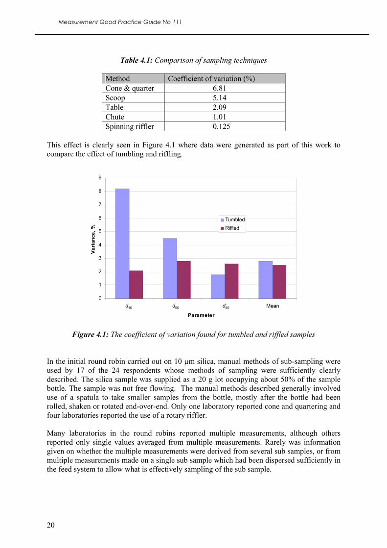
Table 4.1: Comparison of sampling techniques

Method Coefficient of variation (%) Cone & quarter 6.81 Scoop 5.14 Table 2.09 Chute 1.01 Spinning riffler 0.125

This effect is clearly seen in Figure 4.1 where data were generated as part of this work to compare the effect of tumbling and riffling.

0

1

2

3

4

5

6

7

8

9

d10 d50 d90 Mean

Parameter

Var

ianc

e, %

TumbledRiffled

d10 d50 d90

0

1

2

3

4

5

6

7

8

9

d10 d50 d90 Mean

Parameter

Var

ianc

e, %

TumbledRiffled

d10 d50 d90

Figure 4.1: The coefficient of variation found for tumbled and riffled samples

In the initial round robin carried out on 10 µm silica, manual methods of sub-sampling were used by 17 of the 24 respondents whose methods of sampling were sufficiently clearly described. The silica sample was supplied as a 20 g lot occupying about 50% of the sample bottle. The sample was not free flowing. The manual methods described generally involved use of a spatula to take smaller samples from the bottle, mostly after the bottle had been rolled, shaken or rotated end-over-end. Only one laboratory reported cone and quartering and four laboratories reported the use of a rotary riffler. Many laboratories in the round robins reported multiple measurements, although others reported only single values averaged from multiple measurements. Rarely was information given on whether the multiple measurements were derived from several sub samples, or from multiple measurements made on a single sub sample which had been dispersed sufficiently in the feed system to allow what is effectively sampling of the sub sample.


21

4.2 Powder dispersion 4.2.1 Creating a suspension Having obtained what should be a representative powder sample, the particles in the sample must then be dispersed in the medium used by the measurement technique to convey the particles to the active part of the equipment. The majority of equipment used in the round robin studies involved dispersion in water; a few systems used an air flow to convey the powders. Dispersion can involve both the separation of particles from each other and subsequently maintaining both this separation and the suspension of all the particles within the transport medium. Completely dispersing a powder without introducing segregation and ensuring separation of agglomerated particles without breaking up whole particles can be a complex task; part of the complexity arises from a difficulty of knowing when a powder sample is fully dispersed without having broken large particles into smaller sizes. Forces of attraction between particles which lead to agglomeration rise rapidly below 10μm in size, so the finer the sample the greater the problem becomes to separate all the particles. Dry/air dispersion methods rely on shearing and collisions to overcome agglomeration, whereas liquid based methods can use the interactions between the liquid and the solid surface to separate particles and minimize the mechanical forces needed. However the fact that there is a solid-liquid interaction means that care must be taken not to modify the powder most obviously by dissolution. The liquid-solid interaction can be modified by the use of additives (often called dispersants or dispersion agents) as well as by simply changing the liquid itself; these additions can alter the surface tension or reduce the tendency for dissolution. The following procedure is often found to be successful for preparing a powder for liquid (water) dispersion. Take a sub sample and place in a flat-bottomed container; then add appropriate dispersant to the powder, drop wise, until a smooth paste is formed (similar in consistency to toothpaste). A small quantity of the paste is then taken on the tip of a spatula and placed in the cell. The movement of the water washes the sample from the spatula. It is worth noting that the obscuration will rise slowly and time must be allowed for this (see section 4.3). Commonly a sample is made into a thin suspension from which an aliquot is then taken with a pipette. However, as shown in Figure 4.2 sedimentation is then likely and depending upon where the pipette is placed within the container holding the fraction sampled will vary. If this is used the suspension/dispersion in the system needs to be maintained either by pumping or stirring in a holding bath to prevent the samples settling.


22

Fine Fraction Middle Fraction

Large Fraction

Figure 4.2: Schematic showing the settling behaviour of particles in liquids The majority of work in the round robin studies involved dispersion in water. Any optically transparent liquid can be used as the dispersion medium so long as the refractive index is known. Points to consider when choosing and using a dispersion medium are:

• Thermal stirring effects. This is observed when a cold solvent enters a warm cell; time should be allowed for everything to reach equilibrium before a background measurement is taken.

• High vapour pressure solvents (e.g. chloroform) always require the use of a solvent

trap as this prevents evaporation of the solvent which will help the stabilisation of the background readings.

• One key feature to choosing the correct solvent is compatibility with the

instrumentation. For example acetone often damages key seals within the system. Any tubing is also at risk of prolonged use and may need to be fully tested before use.

• When changing from one solvent to another it is advised to do a staged change over.

For example changing from water to hexane. Hexane and water are incompatible and as such will create a gel like emulsion which will take a lot of work to clean out, where as stepping from water to propan-2-ol to hexane will ensure a clean transition between dispersants. Compatibility tables are available from solvent manufactures.

• The density of the powder: At high densities, powder sedimentation in water might be

an issue. In such circumstances like this, use of a more viscous liquid phase might be appropriate. For example, glycerol or water glycerol mixes.

In summary, Figure 4.3 shows a flow chart which neatly summarises the decision steps that might be taken to ensure dispersion.


23

Take representative sample (mix w ell or riff le if dry powder)

Sample

Yes NoDoes it disperse in

water?

Yes

Yes

Yes

No

No

No

Does it f loat?

Does ultrasound

work?

Try a surfactant

Does this disperse it?

Ultrasound if necessary

Analyse

Analyse

Analyse

Analyse


Try solvent, e.g. Ethanol, Propan-2-ol,Methanol, Acetone,

Butanone (Methyl ethyl ketone), Hexane,

Toluene, Dimethyl digol


Take representative sample (mix w ell or riff le if dry powder)

Sample

Yes NoDoes it disperse in

water?

Yes

Yes

Yes

No

No

No

Does it f loat?

Does ultrasound

work?

Try a surfactant

Does this disperse it?


Analyse

Analyse

Analyse

Analyse


Try solvent, e.g. Ethanol, Propan-2-ol,Methanol, Acetone,

Butanone (Methyl ethyl ketone), Hexane,

Toluene, Dimethyl digol


Figure 4.3: Flow chart for deciding how best to disperse an unknown powder (courtesy Malvern Instruments). 4.2.2 Control of solid-liquid interactions Zeta potential: Zeta potential recognises that when a powder is dispersed in water, a surface charge often arises on the surface. This can arise from, for example de-protonation. A silica particle, for example, contains Si-OH groups at the surface that lose a proton in water to form Si-O-. A negative charge results on the silica particle and the release of protons renders the water slightly acidic. The higher the surface charge on the particle (regardless of whether this is positive or negative) the more particles will stay apart or dispersed. This is because the surface charge leads to the creation of a double layer of oppositely charge ions around it. Some ions will be adsorbed to the surface, then other electrolyte ions in the water will be attracted towards the surface. The larger this double layer, the more it acts as a barrier against Van der Waals attractive forces and so agglomeration. The surface charge can be determined by measuring (in mV) the zeta potential. A variety of techniques are used to measure zeta. For example, light and acoustics can be used to monitor charged particle movement under the influence of an applied electric field.


24

If an instance arises whereby difficulties are experienced de-agglomerating a powder in water, ultrasonics should be trialled. Where this fails, it is recommended that the zeta potential versus pH characteristics are measured. Figure 4.4 shows a typical plot for alumina (with and without surfactant) and silica.

-60

-40

-20

0

20

40

60

80

100

0 2 4 6 8 10

pH

Zeta

pot

entia

l [m

V]

Alumina

Alumina + negatively charged polymeric dispersant

Silica

Figure 4.4: Effect of pH on zeta potential.

As a general rule, a powder dispersion in water is considered stable when the zeta potential is greater than +30 mV or less than –30 mV. This means that either a negative or a positive surface charge can be used to ensure deflocculation and so a good dispersion for particle size measurement. If we consider alumina in water (blue diamonds in figure 4.4) it will be seen that stable dispersions (+30 mV and above) exist in the acidic range and up to a pH of ~7.5. Thus, changes in pH can be used to ensure stability. However, where fluctuations in pH are of concern (e.g. chemical attack of components in particle size measuring apparatus), use of surfactants is a preferred option. In Figure 4.4, the pink squares show the zeta potential vs. pH characteristics for the same alumina material coated in an anionic polymeric surfactant. The presence of COO- groups on the polymer confer a negative surface charge and stability (at greater than –30 mV) over the pH range from ~6 upwards. In contrast to alumina, silica when dispersed in water has a largely negative surface charge (see yellow triangles in Figure 4.4). This confers stability at pH values greater than 3.5. If desired, silica could be made stable via a positive zeta potential. This could be achieved by adding a surfactant with a positive charge, for example, one base on a quaternary ammonium salt (NR4

+). The zeta potential vs. pH plot would then become similar to that for alumina. It should also be noted that buffering agents can be added where pH values above or below a given value cannot be tolerated. Such agents will fix pH, whilst surfactants can still be


25

employed to alter the surface charge (and so degree of deflocculation) in the dispersed powder. It should be noted that zeta potential is irrelevant for dispersions featuring hydrophobic solvents. As the polarity of the solvent decreases, it is better to consider steric surfactants to discourage particle / particle interactions and so agglomeration. General dispersants: Dispersants can be divided into three types: Electrosteric, Electrostatic and Steric. The first of these are adsorbed onto the dispersed powder surface to alter (usually increase) the surface charge and so zeta potential. Steric surfactants are branched polymers that adsorb on the powder surface and achieve particle / particle separation not by charge effects but rather by virtue of the space they occupy around particles. Electrosteric additives are something of a half-way house. Water Quality: Again, water quality will have a link to zeta potential and so the ability of particles dispersed in water to remain separated. Tap water will contain electrolyte ions that contribute to the double layer. As the electrolyte concentration increases, this can reduce the size of the double layer (especially if there are 2+ and 3+ ions like calcium, aluminium present). This is because the particle surface charge will be negated by the counter-ions at a shorter distance from the surface. 4.2.3 Maintaining a dispersion in the measurement system In many cases a sub sample is taken and dispersed in a container prior to introduction (as a dispersion) to a container forming part of the measurement system. A number of issues need to borne in mind at this point. i) If the sub-sample dispersion is dilute and very fluid, there is a danger that

sedimentation of the larger particles within the dispersion will occur resulting in the sub-sample introduced to the measurement system having an unrepresentative level of fines and medium grains. This was observed to occur in a number of cases in the round robin where a large volume/dilute dispersion was created and only a small part of this volume then sampled by pipette and added to the measurement equipment. Creation of a paste dispersion gives more reliable results in that homogeneity / dispersion is achieved without providing an opportunity for sedimentation.

ii) The suspension/dispersion in the system needs to be maintained either by pumping or stirring in a holding bath and pumping.

iii) The sample size and settings above will partly be dictated by the need to control the concentration of particles in the measurement system. For laser diffraction, this concentration is controlled to give the correct obscuration level (see 4.3.2).

4.2.4 Effect of density While sedimentation methods rely on the rate of settling of powders dependent on their density and size, for other methods it is essential to maintain all the powder particles in suspension, and this becomes more difficult with powders of very high density. Increased agitation of the dispersion using more ultrasonic power or greater stirring rates is often employed in such circumstances but this approach must be used circumspectly. Too great a use of ultrasonics can cause air bubble formation in liquids, particularly in the


26

presence of some dispersant agents, with the bubbles subsequently detected as particles. Excessive ultrasonics can also raise the suspension temperature (possibly encouraging dissolution and so altering particle size distributions) and damage polymeric surfactants employed to ensure deflocculation – see also section 4.3.1. As mentioned in earlier sections, excessive agitation can cause break up of fragile larger particles, which can also apply to use of very high air pressures. Adding, for example, 10% glycerol to water can help with dense powder particles by increasing the viscosity of the suspending media. Note that by deviating from 100% water as a solvent, the ability to rely on powder surface charge for particle-particle separation reduces. Where non-aqueous solvents are employed, polar materials like glycerol will allow some powder surface charging to take place. 4.3 Measurement The previous section described the issues involved in the dispersion of the powder particles in a suspension up to the point where the measurement system takes the suspension from its holding batch and feeds it through the active measurement cell itself. The following sections briefly describe how to obtain a stable reading. 4.3.1 Use of ultrasonics to control dispersion in liquids Ultrasonic power is an option frequently available for use with liquid dispersion once an aliquot has been added to the measurement system. By causing cavitation in the liquid, the energy of rapidly expanding air bubbles can help separate agglomerated particles and agitate the liquid to maintain a suspension. However, with some combinations of particle size/type and liquid, the ultrasonic process can also cause re-agglomeration, and if used for long times, heating effects may affect sensitive powders. If using ultrasonic power on an unknown powder it is therefore advisable to measure particle size distributions as a function of time and/or power using a trend plot (as shown in 4.3.3). A rapid decline followed by a levelling off of size fractions may indicate good conditions with de-agglomeration and then maintenance of the suspension. A continuous decline may however indicate particle break up, and conversely a continuous rise may indicate agglomeration. Using data from the round robins, Figure 4.5 clearly demonstrates that the application of ultrasound for 30 seconds has had a significant effect on the particle size distribution obtained with a very clear breakdown of large agglomerates.


27

0

1

2

3

4

5

6

7

8

9

10

0.01 0.1 1 10 100 1000 10000

Particle Size (µm)

% V

olum

eNo sonication

50% Sonication powerfor 30 Seconds

Figure 4.5(a): The influence of ultrasound on the particle size distribution of tungsten.

carbide.

0

2

4

6

8

10

12

14

16

d10 d50 d90 d10 d50 d9010μm Silica 100μm Silica

Varia

nce

(%)

Without ultrasonicsWith ultrasonics

Figure 4.5(b): The influence of ultrasound on consistency of results. 4.3.2 Particle concentration It is critical that the signal to noise ratio is acceptable during sample measurement. This will be indicated by the obscuration level (see section 2). Different appropriate levels of obscuration are given by different instrument manufacturers. A minimum level of obscuration is typically around 5% with a maximum of 35%; the obscuration level is very dependant on the sample and its particle size. A small particle will diffract a greater portion of the light thus requiring a lower obscuration level when compared to a much larger particle which will only diffract a small quantity of light. Getting this balance wrong may lead to multiple scattering; an effect where the light is scattered by more


28

than one particle leading to a lower reported particle size. The ISO guidelines are <20µm: 5-15%; >20 µm: 5-35%. The obscuration effect is demonstrated in Figure 4.6. The background (red graph) needs to be overcome to prevent measurement of the background. The schematic demonstrates that as the obscuration is increased, the influence of the background can be minimised. At 11% a good scattering level has been achieved, whereas at 35% multiple scattering effects are observed. The data shown in Figure 4.7 clearly demonstrates multiple scattering effects at high obscuration in 0-10 μm particle size SiO2.

0

20

40

60

80

100

120

1 4 7 10 13 16 19 22 25 28 31 34 37 40 43 46 49 52

Detector numbers

Ligh

t ene

rgy

[a.u

.]

35% Obscuration

11% Obscuration

2% Obscuration

Background

Figure 4.6: The importance of obscuration shown schematically.

0

1

2

3

4

5

6

7

8

9

10

0.01 0.1 1 10 100 1000

Particle size (µm)

% V

olum

e

2% Obscuration

4% Obscuration

8% Obscuration

11% Obscuration

14% Obscuration

17% Obscuration

21% Obscuration

35% Obscuration

50% Obscuration

Figure 4.7: The effect of obscuration on the 0 - 10 μm SiO2.


29

4.3.3 Measurement time & number of measurements The measurement time and number of measurements taken is dependant on the developed method and the time available for the analysis. In practice a measurement is initially taken of the clean dispersant which is then zeroed out of the measurement. Background measurements should be twice the time of the sample measurement time. So a measurement time of 10 seconds would need a background of 20 seconds (up to 30 seconds maximum). During sample measurement, if the material is changing very quickly within the cell then you will need to run quick measurements whereas if you are looking at a sample with a small number of larger particulates then you may need to increase the measurement time to ensure they are all measured consistently over your run time. Figure 4.8 demonstrates the settling of large particles with time in the measurement cell.

0

10

20

30

40

50

60

70

1 3 5 7 9 11 13 15 17 19 21 23 25 27 29 31 33 35 37 39 41

Measurement Number

Appa

rent

par

ticle

siz

e [µ

m]

d10

d50

d90

Figure 4.8: Stability effects of large particles with measurement time.

It is recommended in ISO 13320-1 that 10 measurements are taken per aliquot, the d10, d50 and d90 values are taken and an average, standard deviation and coefficient of variation calculated. The standard states that the d10 and d50 should have a coefficient of variation not exceeding 5% while the d50 should not exceed 3%. This ensures good correlation between measurements and confidence within the run. Figure 4.9 demonstrates this graphically and Table 4.2 illustrates the numerical consistency. It is always good practice to run several aliquots of the same powder.


30

0

20

40

60

80

100

120

1 2 3 4 5 6 7 8 9 10

Measurement number

Para

met

er n

umbe

r (µm

) d10

d50

d90

Figure 4.9: Trend plot data for 0-100μm SiO2.

Table 4.2: Statistics for repeat measurements on 0 – 100 μm SiO2.

Record Number d10, µm d50, µm d90, µm Sample B Run 1 7.248 42.070 109.020 Sample B Run 2 7.276 42.502 110.143 Sample B Run 3 7.288 42.612 109.691 Sample B Run 4 7.287 42.660 109.775 Sample B Run 5 7.243 42.500 110.017 Sample B Run 6 7.260 42.712 110.849 Sample B Run 7 7.247 42.608 110.755 Sample B Run 8 7.215 42.357 109.563 Sample B Run 9 7.241 42.642 110.192 Sample B Run 10 7.122 41.790 109.485 Average 7.243 42.445 109.949 Standard deviation 0.048 0.297 0.566 CV, % 0.664 0.700 0.515

4.3.4 Optical model All laser diffraction software packages provide an option to select an optical model. For the majority of measurements, the general purpose model for polydisperse non-spherical materials is used. Single mode, monomodal distribution is used for the analysis of monomodal characterisation lattices (standard latexes) provided the peak is less than 1 decade in width. Typically these are not natural samples and as such the use of this with other samples will provide a very different result.


31

Multiple narrow mode is used as an extension to the single mode in that it is used to resolve extremely narrow peaks from a mixture of latex lattices. Again, if this is used with samples that have a wide distribution the result will be compromised. As a general rule of thumb it is always advisable to use the general purpose model unless measuring standard latexes or materials that exhibit a very narrow distribution. Remember that you can always edit the data afterwards and this should be taken into account during the method development process. 4.3.5 Refractive index In laser diffraction there are two widely used theories: Fraunhofer and Mie theory, both of which are described fully in ISO13320. The standard also describes in detail the effects of using the different models and of selecting the correct refractive index. In this project the vast majority of the participants who used laser diffraction selected Mie theory. The relative merits of each model are not discussed here, other than to state that Fraunhofer theory breaks down below 2 µm and so caution needs to be exercised comparing data between the two models at particle sizes less than 2 µm. Figure 4.10 compares the effect of using the Fraunhofer theory with that of using the Mie theory on averaged results from the first round robin on 10 μm silica powder described in section 5. Clearly more instruments used Mie theory than Fraunhofer, and partly because of this a wider range would be expected. It should be noted though, that for this powder, with a relatively small fraction of sub 1 μm particles, the approximations of the Fraunhofer theory do not introduce any systematic error that is significant in comparison with other sources of variation.

Figure 4.10: Comparison of size fractions measured by different equipment in the first round robin on 10 μm silica powder using Fraunhofer and Mie theory.

0

2

4

6

8

10

12

F F F F F F F F F F M M M M M M M M M M M M M M M M M M M M M M M M M M M M M

Measurement Type (F = Fraunhofer, M = Mie)

App

aren

t par

ticle

siz

e ( μ

m)

d10

d50

d90


32

For the Mie theory there are many sources of data for the real refractive index (e.g. ISO 13320) but there will be slight differences between sources, for example because of the use of different wavelengths, and this can lead to differences in powder size distributions. Figure 4.11 shows individual distributions measured using two refractive indices on the same sample batch in a single piece of equipment, clearly showing the increase in fine fraction resulting from use of a lower refractive index.

(a)

Malvern Mastersizer 20000-10um Dust Samples A-E

Modal C - 1.53/0.01

0

1

2

3

4

5

6

7

8

9

0.01 0.1 1 10 100 1000 10000

Particle Size Distribution (um)

% F

requ

ency

A B C D E

(b)

Malvern Mastersizer 20000-10um Dust Samples A-E

Modal A - 1.46/0.01

0

1

2

3

4

5

6

7

8

0.01 0.1 1 10 100 1000 10000

Particle Size Distribution (um)

% F

requ

ency

A B C D E

Figure 4.11 (a, b): Different distributions obtained from the same data set, but using different refractive indices (1.53 in (a) and 1.46 in (b)).


33

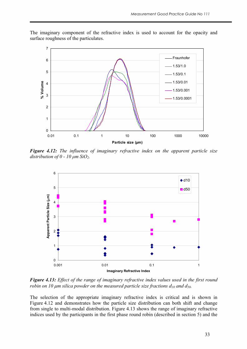
The imaginary component of the refractive index is used to account for the opacity and surface roughness of the particulates.

0

1

2

3

4

5

6

7

0.01 0.1 1 10 100 1000 10000

Particle size (µm)

% V

olum

e

Fraunhofer

1.53/1.0

1.53/0.1

1.53/0.01

1.53/0.001

1.53/0.0001

Figure 4.12: The influence of imaginary refractive index on the apparent particle size distribution of 0 - 10 μm SiO2.

Figure 4.13: Effect of the range of imaginary refractive index values used in the first round robin on 10 μm silica powder on the measured particle size fractions d10 and d50. The selection of the appropriate imaginary refractive index is critical and is shown in Figure 4.12 and demonstrates how the particle size distribution can both shift and change from single to multi-modal distribution. Figure 4.13 shows the range of imaginary refractive indices used by the participants in the first phase round robin (described in section 5) and the

0

1

2

3

4

5

6

0.001 0.01 0.1 1

Imaginary Refractive Index

App

aren

t Par

ticle

Siz

e ( μ

m)

d10

d50


34

corresponding range of results obtained (without separating out the effect of other variables on the results). 4.3.6 Electrozone sensing Producing the correct sample dilution is important in electrozone sensing (EZS) in order to avoid counting multiple particles as a single large particle. EZS equipment can estimate the chances of this happening, reporting it as a coincidence percentage and compensating for this. The following Figure 4.14 shows that for some powders the importance of coincidence has a greater influence on the results than for others. Since the EZS equipment will compensate for the coincidence level measured, it is important to understand both the effect of increased measured coincidence and, by comparing raw and compensated data, its effect on the final results Figure 4.15

4.00

4.25

4.50

4.75

5.00

5.25

5.50

0 10 20 30 40 50 60

Coincidence [%]

d50

[µm

]

Silica AWC A

Figure 4.14: Coincidence vs. d50 data for silica A and tungsten carbide A


35

21

22

23

24

25

26

0 10 20 30 40 50 60

Coincidence (%)

d 50

(mm

)Raw result

Compensated forcoincidence

Figure 4.15: A comparison of raw and compensated data for tungsten carbide B 4.3.7 Optical examination for confirmation It must be strongly recommended that any powder sample subject to size measurement should also be viewed under a microscope, preferably before further measurement. For particles in the range 1 – 100 µm, an optical microscope with a 50× objective for 500× image magnification is sufficient for a brief assessment. The main reasons for optical examination are, firstly, that it confirms the approximate size range to be measured, although it must be realised that a visual check will tend to give an indication of the number mean rather than volume mean. Secondly, as explained in Section 2, particle size measurement techniques make assumptions about the particle shape in order to report a single diameter value for each particle, normally the equivalent sphere diameter; and an optical examination will reveal if this assumption is likely to be a reasonable approximation or a poor estimate because, for example, the particles are rod like.


36

6Variability of Results: Outcome of Round Robin Studies

IN THIS CHAPTER

55

Comparison of Interlaboratory Measurements of Silica Powder Sample Distributions


37

5 Variability of Results – Outcome of Round Robin Studies 5.1 Introduction To provide background information for this guide, a series of round robin tests were carried out with a range of powder types and with a range of laboratories (ranging from instrument manufacturers through industrial users, general test laboratories and universities). The full results of these tests are described in a separate report 2. In this chapter a summary of the data is given for just a few of the tests in order to show the reduction in variability that can be obtained by determining a sample preparation and analysis procedure that can be implemented over a wide variety of equipment. 5.2 Round robin structure The two powders that were analysed in round robin stages at both the start and the end of the programme were the crystalline Silica “A” and “B” powders, with maximum sizes of approximately 10 μm and 100 μm respectively. Since the initial objective was to establish current practice for sizing of an unknown powder with the minimum of influence from the organisers, participants were given the minimum amount of information on the Silica “A” powder; a chemical hazard sheet and a return sheet which sought to capture the exact procedure used. For Silica “B” the real refractive index was given and specific questions were asked about the method used, but otherwise the analysis procedure was again left to the participants’ discretion. Approximately 12 months later, the same powders were distributed, but with labels Silica “C” and “D” in place of “A” and “B” respectively. A much more detailed procedure was now specified within the limitations of allowing for the different equipment used by the participants. In particular, the method of dispersion was stated specifically to be based on making a paste with a defined amount of powder and adding the paste to the equipment tank with a minimum quantity of water without use of ultrasonics or dispersants. A minimum obscuration level and number of repeat readings were specified. Full details are given in Appendix 4. 5.3 Comparison of starting and final round robins Figure 5.1 plots results for the particle size fractions to give an indication of the level of scatter in results obtained for the first round Silica “A” and “B” where laboratories were free to determine their own procedure. Significantly fewer laboratories participated in the final second round to measure Silica “C” and “D”, so to show the effect of the more prescriptive measurement, Figure 5.2 plots the results of both first and second rounds by laboratory number. The reduction in spread of results can be quantified by comparing the change in the coefficient of variation for each size fraction. Table 5.1 shows the mean, standard deviation and coefficient of variation for each size fraction from the first round with Silica “A” and “B” (column headed RR1) and the second round with Silica “C” and “D” (column headed RR2).

2 NPL Report MAT XXX “Final Report on Powder Sizing Round Robins”


38

There was an increase in the mean values measured in the second round for both powders and for all size fractions, but more significantly the coefficient variation was reduced substantially in almost all cases. Apart from a slight (8%) increase in the coefficient for the 10 μm silica d90 fraction, decreases of 19, 49 and 53% were obtained for this silica “C”, and even greater reductions in the coefficient of variation for the 100 µm silica powder were noted, three being greater than >50%. The latter result is perhaps expected given the broader distribution of particle sizes and so greater opportunities for preferentially sampling fines or coarser fractions.

Table 5.1: Comparison of results from initial round robin (RR1) and those from the final round (RR2), showing a reduction in the spread of results using

a more closely defined procedure.

d10, µm d50, µm d90, µm d4,3, µm RR1 RR2 RR1 RR2 RR1 RR2 RR1 RR2

Silica “A/C” (<10 µm) Mean size 1.3 1.6 3.3 4.0 8.6 9.3 4.5 5.0 Standard deviation 0.55 0.55 0.68 0.38 0.75 0.88 0.53 0.30 Coefficient of variation, Cv 0.437 0.352 0.204 0.096 0.088 0.095 0.118 0.060% reduction in Cv 19 53 -8 49

Silica “B/D” (<100 µm) Mean size 6.0 6.9 39.0 41.3 102.3 104.1 48.0 49.7 Standard deviation 1.82 0.68 5.45 2.05 7.56 4.76 4.95 2.15 Coefficient of variation 0.305 0.099 0.140 0.050 0.074 0.046 0.103 0.043% reduction in Cv 68 64 38 58

0

2

4

6

8

10

12

110

111

111

112

113

113

115

116

117

117

118

119

121

121

122

122

123

124

125

127

128

129

130

130

131

131

131

131

132

132

132

133

134

135

137

138

138

139

139

140

141

141

Laboratory number

App

aren

t par

ticle

siz

e (µ

m) d10 d50 d90 d4,3

Figure 5.1(a): Results of initial round robin for Silica “A”.


39

0

20

40

60

80

100

120

140

110

111A

111A 11

311

6A11

6B11

8A11

8B 119

121A

121B

122A

122B

122C

122D 12

312

412

512

813

013

1A13

1B13

1C13

1D 133

134

135

137

138A

138B

139A

139B

140A

140B

141A

141B

Laboratory number

App

aren

t par

ticle

siz

e (µ

m)

d10 d50 d90 d4,3

Figure 5.1(b): Results of initial round robin for Silica “B”

0

2

4

6

8

10

12

138 d

ry

138 w

et 139

111

140

125

137

116

Laboratory number

App

aren

t par

ticle

siz

e (µ

m)

d90 (2)

d50 (2)

d4,3 (2)

d10 (2)

d90 (1)

d4,3 (1)

d50 (1)

d10 (1)

Figure 5.2(a): Comparison of results for 10 μm Silica A measured in initial round robin (1) with results for same powder Silica C measured in final round robin (2). Results ordered by increasing d90 for RR2.


40

20

30

40

50

60

70

80

90

100

110

120

111

139

116

138 d

ry 137

138 w

et 125

140

Laboratory number

d90

, d50

, d4,

3 siz

es (µ

m)

0

2

4

6

8

10

12

d10

siz

e fr

actio

n (µ

m)

d90 (2)

d50 (2)

d4,3 (2)

d90 (1)

d50 (1)

d4,3 (1)

d10 (2)

d10 (1)

Figure 5.2(b): Comparison of results for 100 μm Silica B measured in initial round robin (1) with results for same powder Silica D measured in final round robin (2). Results ordered by increasing d90 for RR2.

0

2

4

6

8

10

12

111

138 d

ry

138 w

et 125

137

116

140

139

Laboratory number

Size

frac

tion

(µm

)

d90 (2)

d50 (2)

d4,3 (2)

d10 (2)

d90 (1)

d50 (1)

d4,3 (1)

d10 (1)

Figure 5.2(c): Comparison of results for 10 μm Silica A measured in initial round robin (1) with results for same powder Silica C measured in final round robin (2). Results randomly ordered.


41

Figure 5.2(d): Comparison of results for 100 μm Silica B measured in initial round robin (1) with results for same powder Silica D measured in final round robin (2). Results randomly ordered.

20

30

40

50

60

70

80

90

100

110

120

111

138 d

ry

138 w

et 125

137

140

139

116

Laboratory number

d50

, d90

, d4,

3 siz

e fr

actio

n (µ

m)

0

2

4

6

8

10

12

d 10

size

frac

tion

(µm

)

d90 (2)

d50 (2)

d4,3 (2)

d90 (1)

d50 (1)

d4,3 (1)

d10 (2)

d10 (1)


42

7Recommendations

IN THIS CHAPTER

66

Sources of Information

Reference Powders

Major Practical Issues for Laser Diffraction


43

6 Recommendations It should be clear from this Guide that it is not possible to define a single correct way of measuring the size distribution of an unknown powder. What can be done is to emphasise the need to develop a protocol for each new powder encountered and highlight a number of key factors that should be considered and then fixed for each new protocol. In addition to the practical considerations specific to particle sizing, a number of issues common to many test methods (e.g. training) can be considered and information is given in this section on where to obtain further help. 6.1 Sources of information 6.1.1 Standards A number of international standards are available which give a large amount of information on the factors which should be considered in developing procedures for analysis of unknown powders using particular measurement techniques. They also provide useful background information which explains some of the theory behind the different measurement methods. The following provides a very brief list of the principal topics covered; a fuller list is provided in the bibliography. Particle Sizing Methods BS 8471 Dispersion BS ISO 14887 Sampling - BS ISO 14488 Representation of Particle Size BS ISO 9276-1,-2,-4,-5 ASTM E1617 Laser Diffraction BS ISO 13320-1

ASTM B822 Electrozone sensing - BS ISO 13319 Sedimentation BS ISO 13317 –1, -3 6.1.2 Manufacturers Equipment manufacturers have a wealth of expertise and information which they are generally very happy to share with users of their equipment. Through previous case study work undertaken with a wide range of clients, they will often be able to suggest appropriate dispersion and operating conditions for particular powder types, suitable for the particular equipment in use. 6.1.3 Training Training is an obvious necessity for equipment operators. When new equipment is delivered manufacturers provide a good generalised training which will cover analysis of a range of powder types with enough background knowledge to develop new procedures for new powders. However operators may change, and/or a single standard procedure is used over a long period of time on one or two powders types, such that when a new powder with different properties is presented, the knowledge for selecting suitable new measurement parameters has been lost. There are a number of options that can be considered for training new or even experienced operators:


44

Manufacturers regularly run training courses which will be particularly suited to their own particular operating systems and software.

A number of organisations offer training courses which may be more general and utilise experts from a variety of backgrounds. These include the Particle Characterisation Interest Group of the Royal Society of Chemistry, and the Particle Technology Subject Group of the Institute of Chemical Engineers.

Proficiency testing schemes represent good practice to ensure the ongoing competence of a laboratory. Participation in such schemes involves measurement, to a carefully defined procedure, of samples that have already been comprehensively characterised by a range of experts. Confidential comparison of participant’s results with the mean values and feedback from the experts enables self-assessment and improvement in practice. Currently the PACQS scheme is run by LGC9

When liaising with suppliers and users up and down the supply chain, the importance of recognising that each company is likely to employ different machines, protocols should not be under-estimated. Working together to create a common protocol and then doing trials on a range of common materials to demonstrate correlations is recommended. 6.2 Reference powders It is assumed in the following sections that the particle sizing equipment is properly maintained and aligned correctly. The effects of poor set up, such as misaligned optics, are described in a number of documents (e.g. in standards, NIST Recommended Practice3) and do not need repeating here, but it should be noted that verification that equipment is correctly functioning on a daily or weekly basis may be carried out with reference powders. There are a number of sources of commercially produced reference powders (e.g. individual manufacturers, Whitehouse Scientific10, LGC11 ) but it should be borne in mind that it is very common for these powders to have very different characteristics from an unknown powder that might confront the user. Thus obtaining the expected mean size or size fractions with a reference powder may show that the optical system of a laser diffraction is aligned correctly, but it will not ensure that the results obtained for an unknown powder are correct if the latter has different optical properties from the reference or requires different conditions to produce and maintain a dispersion in the equipment. Many commercially available reference powders are spherical (e.g. latex) and have relatively narrow size distributions and so will require different software models and input parameters from those applicable to an unknown. Some laboratories develop their own reference material, perhaps taken from a production batch with similar properties to their most commonly analysed powders. Such reference powders can provide verification of continued equipment performance over a wider range of sizes, and can be useful in internal comparisons between different pieces of equipment or different operators. However some obvious precautions need to be taken with such reference powders, such as ensuring that the powder is stable over time, and does not segregate during storage or sampling. Moisture pick-up can increase the tendency to agglomerate, and oxidation can change the powder properties. 9 www.lgcpt.com/scheme.aspx?SchemeID=136 3 see p6. 10 www.whitehousescientific.com 11 www.lgc.co.uk


45

6.3 Major practical issues for laser diffraction Based on the results of the round robin studies described in the previous section, a number of key issues that contribute to variability can be highlighted. 6.3.1 Sampling Most laboratories do not have access to the ideal method for sampling, riffling, which gives the most reproducible methodology. However the results described in section 4.xx clearly show that selection of the best alternative methods can substantially improve the reproducibility of results. 6.3.2 Initial dispersion of sample The biggest factor in reducing the spread of results that has been demonstrated by the round robins described in this Guide is the method employed when initially introducing and dispersing the powder in the measurement system. It is very easy to allow sedimentation at this point which results in a consistent bias to subsequent measurements. 6.3.3 Maintaining a stable dispersion It is vital when determining the procedure for a new powder to determine that the conditions chosen give a stable result; the absence of stability (manifested as a drift in PSD as repeat measurements on a single aliquot are made) is a reliable indication that the dispersion conditions have not been sufficiently optimised and that, for example, agglomeration, break-up, or dissolution is occurring while the sample is being analysed. 6.3.4 Refractive Indices Use of the correct refractive index becomes important for analysis of particles with size approaching the wavelength of the laser light used. However, it can be seen from the data collected from the round robins described in this Guide, that for these types of powders, the other factors listed above can have an equally large influence on the measured size distribution. Agreeing fixed values for both real and imaginary indices is however a first step to minimising variability. Overall, addressing these and other issues in Round Robin 2 (where prescriptive instructions for particle size distribution were given and adhered to) resulted in a reduction of approximately 50% in the coefficient of variation for most particle size fractions


46

8Appendix 1

IN THIS CHAPTER

77

A simple checklist for particle size measurement


47

Appendix 1: A simple checklist for particle size measurement The following table is designed as a quick aide-memoire to remind staff undertaking PSD measurements of the main factors that can influence results. Having considered these factors, users are encouraged to define their own protocols for PSD measurement by filling in column 5. The table is not exhaustive and is based on the 80/20 principle to provide quick “at a glance” guidance to improve PSD measurement. It does not seek to instruct the user on what is “right” or “wrong”. In some instances it points out preferred options but ultimately it is up to the user to decide the approach taken (recognising that decisions may be constrained by factors such as availability of equipment). The table will have achieved its goal if users ultimately define and then rigorously apply their own protocol. Encouraging companies immediately up or down the supply chain to also discuss / adopt a common protocol is also important and this table should assist the process. Column 1 lists (in order) the generic steps involved in making a PSD measurement. Column 2 then lists sub-steps, whilst column 3 flags up some considerations at each sub-step. Column 4 suggests options for delivering each sub-step using numbering, i.e. (i) = best approach; (ii) = next best approach, etc. In someinstances colour shading is for guidance: green for a “sound approach”; yellow for an “acceptable approach but watch for pitfalls” and amber for “best avoided”. Having digested the information in Columns 1-4, the user is then encouraged to create their own procedure in the empty column 5. As a word of caution, this table is designed specifically for users of laser diffraction measurement equipment. Whilst users of other techniques will find information relating to Steps 1 and 2 fully relevant, aspects of Steps 3 and 4 will be irrelevant. The hope is that the methodology will also be of use to users of sedimentation and electro-zoning techniques, etc.


48

STEP SUB-STEP CONSIDERATIONS OPTIONS MY CHOSEN PROCEDURE

* Maybe the sample has agglomerated due to moisture adsorption over time?

* Agree measurements at different labs are conducted after a fixed time. * Store samples in dry conditions. * Subject sample to drying / light pestle & mortar action before measurement. CAUTION – possible primary particle breakdown.

* Taking into account the sample / sub-sample history.

* Has separation of fines and coarse fractions occurred during transport?

* Consider re-mixing sub-sample by tumbling in its sample tube immediate prior to measurement.

* Bulk sampling. * Securing a representative sample: has separation of fine and coarse fractions occurred (e.g. during transport or whilst stored in a silo)?

* Take sub-samples from multiple positions in still bulk sample and re-combine or….. * If dry powder flows as part of the production / delivery process, take samples at different times, positions and combine. * Avoid sampling from a heap as fines and coarse particles tend to separate.

* Sub-sampling. Securing a representative sub-sample. i) Riffling: Not so good for powders with poor flow. ii) Cone and quartering: Good for powders with poor flow. iii) Tumble in container / spatula. iv) Spatula.

Powder sampling / sub-sampling

* Alliquots. Suspension preparation prior to introduction to cell.

(i) Creating a paste: Best approach, as powder / air interfaces are removed, and sedimentation is not possible. (ii) Creating a fluid suspension in a beaker and using a pipette to transfer to cell can result in large particles quickly sedimenting in the beaker and not being picked up in the pipette. A PSD with smaller particles dominating results. (iii) Simply throwing powder into the liquid phase in cell could result in the powder taking a considerable time to de-agglomerate or never fully breaking down to primary particles.


49

STEP SUB-STEP CONSIDERATIONS OPTIONS MY CHOSEN PROCEDURE * Dry powder measurement. Ensuring agglomerates are fully

broken down to dry primary particles. (i) Employ silo emptying / vibrating chute / compressed air mixing, etc., to encourage regular feed rate and de-agglomeration. Best employed as part of the measurement process, rather than an action prior to introduction to machine. Carry out calibration work whereby PSD is measured as a function of intensity of de-agglomeration. This allows user to identify ideal conditions for de-agglomeration but avoiding milling. (ii) Pestle and mortar – Employ to gently break down agglomerates. CAUTION: Possible primary particle break down. (iii) Doing nothing means there is a risk of agglomerates not breaking down and PSD appearing coarser.

* Do I use water or other liquid as dispersing media?

* Using denser liquids such as glycerol (along or mixed with water) can reduce sedimentation when measuring higher density powders like Ni, WC. * Check sample is not soluble in water and seek less polar solvents if this is the case.

Powder Dispersion

* Wet suspensions.

* Tap or distilled water?

(i) Distilled water (ii) Tap water. The soluble ions in tap water (electrolyte) can influence zeta potential and hence how well dispersed the powder in the suspension is ref. Generally, higher electrolyte concentration and the presence of 2+ or 3+ ions (like Ca2+, Al3+) will encourage unwanted flocculation.

Measurement (I): Fixing soft-ware settings.

* Refractive Index * Imaginary RI

* Changes in RI can dramatically alter the final PSD (e.g. the PSD can appear mono or bi-modal) where MIE theory is employed * Changes in this value can alter whether the PSD is broad or narrow

* Measure RI of the sample and use value. * Agree a common literature RI value to use. * Use SEM analysis to get an idea of whether PSD is actually broad or narrow. Apply a fixed appropriate Imaginary RI value (as this value rises from 0.01 to 1.0, the PSD narrows * Agree / fix any imaginary RI value to use


50

STEP SUB-STEP CONSIDERATIONS OPTIONS MY CHOSEN PROCEDURE * Pump speed / rate * Does my instrument use MIE or Frauenhofer calculations? * Does my instrument have other methods for coping with smaller particles? * Can the equipment offer corrections for particle shape?

* Energy put into mixing can affect quality of de-agglomeration and (with excess energy) even agglomeration. Watch for temperature increases that alter level of solubility of dispersed powder. * MIE and Frauenhofer both have a particle size range that they can cope with * Some instruments can bring an alternative detection mode into play to better measure fines (e.g. use of polarised light) * Shape will influence laser diffraction patterns with software simply calculating a sphere equivalent size

* Compare flow rates, pump power and time of mixing for different models/manufacturers of equipment. Carry out calibration checks (how does PSD change versus mixing time?) Identify, then nominate, a protocol for different laboratories / machine that results in a comparable energy input. * For powders with a significant level of fines, Frauenhofer theory (which can deal with sizes down to 2 µm) may not be suitable. Mie theory can cope with 0.1 µm upwards. Select Mie or Frauenhofer theory option accordingly if available. * Decide whether additional modes will / will not be used and introduce decision into protocol. * Again, decide on whether to select or avoid correction factors based perhaps on SEM analysis.

Measurement (II): Fixing other variables

* Checking equipment performance prior to measurement

* Background runs (made with solvent only in the cell) allow determination of very low levels of laser light reaching detectors in absence of diffracting powder. How often do I check this? * Background reading taken is not satisfactory * Calibration run : What material do I select for calibrating?

* Run before each sample is run. * Run according to manufacturers recommend-ations (with built in timing to force user to measure at specified periods). * Run every hour. * Run at the start of each day. * Remove and clean windows, lenses according to instructions to avoid damage to coatings. * Consider pumping cleaning agent in water in between measurements. * Air bubbles may be present – circulate water for longer period / avoid vigorous circulation and re-check background. * Mono-sized glass spheres (avoids variations in data due to shape) with narrow PSD. Run once a month. * Secure other non-spherical “reference” and run monthly.


51

STEP SUB-STEP CONSIDERATIONS OPTIONS MY CHOSEN PROCEDURE * Level of aliquot added during a measurement * Use of ultrasound * Use of surfactants * Use of electrolytes and / or pH * Number of measurements per aliquot * Number of aliquots to run tests on.

* Optical alignment check * Don not add to little or too much. Too much risks multiple scattering of light and erroneous results. Too little means not enough scatterings to give statistically meaningful data. * I only have a limited amount of powder to disperse. * Can assist in reducing agglomeration. * Can assist in reducing agglomeration. * Can assist in reducing agglomeration in aqueous systems * By running repeat measurements, you can check for trends in PSD associated with the sample gaining greater homogeneity. * Running greater than one aliquot gives more data to ensure a reliable result.

(i) If % obscuration figures are given aim for adding enough sample to deliver the same % figure on every run. (ii) Often equipment offers a “window” or range of acceptable obscuration. Make sure you are in this range. (i) Run measurement at highest % obscuration value below acceptable level. Retain the % as the value always used. * Watch for excess energy input cause agglomeration (manifesting as temperature rise). Worth doing trials to track PSD vs. U/S power setting, U/S time. * For aqueous systems, need to check surfactant is suitable for powder being tested. Zeta potential vs. pH plots for powder and powder + surfactant will assist. A zeta value of > ± 30 mV is recommended. * Monitor zeta potential as function of electrolyte and pH checking for < + 30 mV or > - 30 mV. * Take three measurements if results are almost identical; take five measurements if not. For five measurements ignore the first one or two measurements if subsequent ones are lower and consistent. * Generally not necessary if good consistency seen with first aliquot.


52

STEP SUB-STEP CONSIDERATIONS OPTIONS MY CHOSEN PROCEDURE Issues with the PSD obtained.

* How can I be sure my measured PSD will mean good or bad performance down the processing line? * How should I display the data? * I use a LD unit that represents a different model / manufacturer from the one my supplier / client uses.

* Need to do correlation studies. * Consider what y-axis should be. * Should I display fractional or cumulative PSD? * Need to check that a good correlation between different units exists.

* Apply Factorial Experimental Design (FED) or alternative to show the level of correlation between PSD values (D10, D50, D90 etc.) and intermediate or final products made with different powder batches. (i) Vol.%. The format usually adopted. (ii) Wt.% (i) Number % (good for seeing the presence of fines) – can this be done?? (i) Super-impose both. (ii) Fractional only (good for assessing mono, bi-modal etc. but not easy to see d10, d50, d90, etc.) (iii) Cumulative only (good for quickly identifying d10, d50, d90, etc.) * Carry out PSD runs on a series of standard materials with different PSD, Dispersity. Use the same protocol as you have defined in column 4. Plot d10, d50, d90 and d4,3 data for the two instruments against each other.


53

9Appendix 2

IN THIS CHAPTER

88

Sources of Information


54

Appendix 2: Sources of information on particle size measurement Textbooks: Allen, T.; Particle size measurement, Vol. 1. Powder sampling and powder measurement

Chapman and Hall, 5th edition, 1997. Allen, T.; Particle size measurement, Vol. 2. Surface area and pore size determination,

Chapman and Hall, 5th edition, 1997. Allen, T.; Powder sampling and particle size determination, Elsevier, 2003. Merkus, H. G.; Particle size measurements, fundamentals, practice, quality; Particle

Technology Series, Vol. 17, Springer Verlag, 2008. Syvitski, J.P.M.(ed); Principles, methods and application of particle size analysis,

Cambridge University Press, 1991. Websites: Beckman Coulter Inc. http://www.beckmancoulter.com/products/ Horiba Instruments Inc. http://www.horibalab.com/page.php?id=294 Malvern Instruments Ltd.: http://www.malvern.com/ Matec Inc.: http://www.matec.com/mas/ Meritics Inc.: http://www.meritics.com/index.html Microtrac Inc. http://www.microtrac.com/products.cfm Omec Ltd. http://omec-tech.com/en/Products-01-gs.asp Particle Technology Ltd http://www.particletechnology.com/ Particles CIC, University of Leeds http://www.particlescic.com/ Powder Technology Inc. http://www.powdertechnologyinc.com/ Retsch GmbH http://www.retsch.com Sympatec Ltd. http://www.sympatec.com


55

10Appendix 3

IN THIS CHAPTER

99

Standards for Particle Size Measurement


56

Appendix 3: Listing of standard test methods for particle size measurement ISO Standards BS ISO 9276-1:1998 Representation of results of particle size analysis. Graphical

representation BS ISO 9276-2:2001 Representation of results of particle size analysis. Calculation of

average particle sizes/diameters and moments from particle size distributions BS ISO 9276-3:2008 Representation of results of particle size analysis. Adjustment of an

experimental curve to a reference model BS ISO 9276-4:2001 Representation of results of particle size analysis. Characterization of a

classification process BS ISO 9276-5:2005 Representation of results of particle size analysis. Methods of

calculation relating to particle size analyses using logarithmic normal probability distribution

BS ISO 9276-6:2008 Representation of results of particle size analysis. Descriptive and quantitative representation of particle shape and morphology

BS ISO 13317-1:2001 Determination of particle size distribution by gravitational liquid sedimentation methods. General principles and guidelines

BS ISO 13317-2:2001 Determination of particle size distribution by gravitational liquid sedimentation methods. Fixed pipette method

BS ISO 13317-3:2001 Determination of particle size distribution by gravitational liquid sedimentation methods. X-ray gravitational technique

BS ISO 13318-1:2001 Determination of particle size distribution by centrifugal liquid sedimentation methods. General principles and guidelines

BS ISO 13318-2:2007 Determination of particle size distribution by centrifugal liquid sedimentation methods. Photocentrifuge method

BS ISO 13318-3:2004 Determination of particle size distribution by centrifugal liquid sedimentation methods. Centrifugal X-ray method

BS ISO 13319:2007 Determination of particle size distributions. Electrical sensing zone method

BS ISO 13320-1:1999 Particle size analysis. Laser diffraction methods. General principles (Note that a new extensively revised version of this standard is currently in preparation.) ISO 13321:1996 (BS 3406-8:1997) Methods for determination of particle size distribution.

Photon correlation spectroscopy BS ISO 13322-1:2005 Particle size analysis. Image analysis methods. Static image analysis

methods BS ISO 13322-2:2006 Particle size analysis. Image analysis methods. Dynamic image

analysis methods BS ISO 14488:2007 Particulate materials. Sampling and sample splitting for the

determination of particulate properties BS ISO 22412:2008 Particle size analysis. Dynamic light scattering (DLS)


57

ASTM Standards B215-2008 Practices For Sampling Metal Powders B761-2006 Test Method For Particle Size Distribution Of Metal Powders And Related

Compounds By X-Ray Monitoring Of Gravity Sedimentation B821-2002 Guide For Liquid Dispersion Of Metal Powders And Related Compounds For

Particle Size Analysis B822-2002 Test Method For Particle Size Distribution Of Metal Powders And Related

Compounds By Light Scattering E 1617-97 Practice For Reporting Particle Size Characterization Data Addresses of standards organisations British Standards Institution (BSI): 389 Chiswick High Road, London UK, W4 4AL Phone: (+44) 208 9969000, Fax: (+44) 208 9967400 URL: www.bsi.-global.com International Standards Organisation (ISO): 1, rue de Varembe, Case postale 56, CH-1211 Geneve 20, Switzerland Phone: (+41) 227490111, Fax: (+41) 227333430 URL: www.iso.ch American Society for Testing and Materials (ASTM): 100 Barr Harbour Drive, West Conshohocken, PA 19428-2959. USA Phone: (+1) 610 832 9500, Fax: (+1) 610 832 9555 UK Office: 27/29 Knowl Piece, Wilbury Way, Hitichin, Herts. SG4 OSX. UK Phone: (+44) 1462 437933, Fax: (+44) 1462 433678 URL: www.astm.org


58

11Appendix 4

IN THIS CHAPTER

1100

Powder Sampling Methods


59

Appendix 4: Powder Sampling12 Reliable powder sampling is obligatory for all particle characterisation procedures. The sample collected from the bulk must be representative of the entire physical and chemical characteristics of the system in order for derived data to contain any meaning. According to the ‘Golden Rule of Sampling’: A powder should be sampled when in motion The whole sample stream should be taken over many short time increments, rather

than part of the stream being taken for the whole of the time. During bulk sampling, issues arise due to powder segregation. Variation exists in different regions of a heap or container and also between sample containers. If static sampling must be employed, samples should be taken from many random positions in different bags or containers, and later combined to form as representative a sample as possible. In the case of heap sampling, if possible the heap should be mixed prior to sampling. There are a variety of different sub-sampling methods which can be used to turn a bulk sample into a more manageable laboratory sample. Cone and quartering The powder is formed into a cone shaped heap on a flat surface, before being flattened with a spatula and divided into four identical volumes. One portion is taken and the entire procedure is repeated until only 1/16th of the original volume remains. This method is heavily operator dependant and is only suitable for powders with poor flow behaviour and thus little segregation. Large particles will tend to roll to the outside edges of the heap as it is made, while fine material will adhere to the working surface, thus narrowing the final overall size distribution. Scoop Sampling The operator manually scoops a small portion of powder from the bulk sample. Only appropriate for homogenous materials with poor flow characteristics. Table Sampling The sample moves down an inclined plane, prisms divert and control the flow so that aliquots of sample fall through holes in the table. The powder that is collected at the end of the table is the required sub-sample (Figure A3.1). Initial feed should be representative and mixed thoroughly, to eliminate the main source of variation. Chute The sample is introduced into a V shaped trough, feeding through a number of chutes, and collected in two trays on either side of the trough. The procedure is repeated with the powder in one tray, until the desired amount is obtained. The trough must be loaded without causing sample segregation. 12 Taken from an analytical note produced by ParticlesCIC, © ParticlesCIC 2009


60

Figure A3.1: Table sampling Spin Riffling A spinning riffler (see Figure A3.2) divides the sample into a series of glass containers. Powder is transported from the hopper, via a vibratory chute, into a series of containers rotating at a constant speed. The sample flows into the receivers at a constant rate causing them to be filled uniformly. The drawback to this method is that the sample volume is relatively small, handling powders in grams and milligrams.

Figure A3.2: A spinning riffler

For ease of comparison, a summary of the advantages and disadvantages of each sampling technique is given in Table A3.1.


61

Table A3.1: Sampling technique comparison

Method Advantages Disadvantages Cone & quarter

Good for powders with poor flow characteristics Operator dependent

Scoop Reliable for homogenous and non-flowing powder Particle segregation

Table Separates a large quantity of material Initial feed dependent

Chute Reduce powder sample by half after one pass Operator bias

Spinning riffler

Reliable for free flowing powders

Inability to do large quantities efficiently

A paper by Allen and Khan13 details a study regarding the reliability of each of the sampling devices mentioned in this application paper, the results are given in Table A3.2. It is clearly seen that the spinning riffler is the most reproducible method of sub-sampling, with cone and quartering giving the largest standard deviation.

Table A3.2: Sampling technique reliability

Method Relative Standard Deviation (%)

Cone & quarter 6.81 Scoop 5.14 Table 2.09 Chute 1.01 Spinning riffler 0.125

Summary

• The most reproducible method of sub-sampling is governed by the characteristics of the material.

• Using an incorrect method will result in a particle size distribution not representative of the bulk material.

13 Allen, T.; Khan, A.A.; Critical Evaluation of Powder Sampling Procedures, Chemical Engineer (London), 1970, No. 238, 108–112.


62

12Appendix 5

IN THIS CHAPTER

1111

Round Robin Data Sheets


63

Appendix 5: Round Robin Data Sheets

RETURN SHEET – POWDER #1

Laboratory Number: ..................... Your details: Name of contact person:.......................................................................................................... Name of operator if different: .........................…..(or your own anonymous i.d. if preferred). Organisation: .............................................................................................................. Address: .............................................................................................................. Postcode: ........................................................................................ Tel: ............................................ Fax: ...................................... E-mail: .................................................. Your equipment: Instrument #1 Make: .........................................Model type: ..................................... Age: ............... Instrument #2 Make: .........................................Model type: ..................................... Age: ............... Instrument #3 Make: .........................................Model type: ..................................... Age: ............... Your procedure: 1. Instrument calibration Please describe how your instrument is normally calibrated, and how frequently you do it. If you use a certified reference material, please give details of it and its source: .................................................................................................................................................


64

2. Sampling Please describe how you took a sample from the supplied material: ................................................................................................................................................. 3. Sample preparation Please describe how you dispersed the sample before the test and how you maintained the dispersion up to the start of the test, giving details of all parameters you consider to be relevant: ................................................................................................................................................. 4. Test parameters Please give details (descriptive and numerical) of parameters you would normally record during the operation of a test: ................................................................................................................................................. 5. Computation Please give details of the software employed for the calculation and the source of the theory employed by the software. Please also provide any additional powder-type-specific numerical input parameters required by the software, the actual values you inserted, and where these values were sourced: ................................................................................................................................................. 6. Your results: Please return values of particle size, µm, on a volume basis for d10,d50 and d90, and d(4,3) Instrument #, Run i.d. etc D10 D50 D90 D (4,3) Other notes

7. Format results file Please supply electronically a numerical output file from your instrument. We would prefer an ASCII file if you can produce one, but failing that an instrument software output file Our file is in: ASCII format:......... Machine software format:................................................. Machine software name and version number: ..........................................................................


65

RETURN SHEET

2nd ROUND, SILICA C

Laboratory Number: ..................... 1. Your equipment: Make: ........................................Model type: ......................................... Age: ............... Your procedure: Please follow the procedure below where possible. Please note at any point if you have to do something else/ something extra 2. Sampling Not everyone has access to a riffler. Please therefore use the following method based on that most commonly reported in the previous rounds: Tumble the sample bottle end over end 10 times, and then with a spatula remove

samples from top, middle and bottom of the sample. In line with the standard BS ISO 14488:2007, the minimum weight sampled should be > 0.001 g, but see below for the dispersion method which will probably require more than this.

3. Sample preparation Please do not use a dispersant. Mix the sample above into a paste with toothpaste like consistency by adding

deionised water drop wise to the sampled powder to form a non-settling slurry Add to your equipment tank, ensuring >500ml of deionised water is used to disperse

the paste Please do not use ultrasonics.

4. Test parameters Set pump and stirrer, then add your sample gradually to give an obscuration of

approximately 10%, or if your equipment has an optimum mid range obscuration value that is different, please note here.

Once the sample is fully dispersed, please take 5 consecutive measurements to check that enough time has been allowed to create an homogeneous suspension and so a stable PSD. Please note the time taken to acquire a stable reading and calculate the average. Ideally the work should be completed using at least two aliquots of powder to ensure validation of the result. If you can, please estimate the weight of powder sampled.

5. Computation Please use the following refractive indices: R.I. 1.53. Imaginary: 0.001


66

6. Your results: Please return values of particle size, µm, on a volume basis for d10,d50 and d90, and d(4,3) Instrument #, Run i.d. etc D10 D50 D90 D (4,3) Other notes

7. Format results file If possible, please supply electronically a numerical output file from your instrument. We would prefer an ASCII file if you can produce one, but failing that an instrument software output file Please return the form and your output data file to: Ken Mingard or Roger Morrell at National Physical Laboratory, Hampton Road, Teddington, Middlesex, TW11 0LW, UK E-mail:[email protected] Fax: +44 20 8943 2989

Date post:	02-May-2018
Category:	Documents
Upload:	lydang
View:	214 times
Download:	1 times

Improving the consistency of particle size measurement€¦ · · 2017-08-01Good Practice Guide...

Documents