IMPROVING THE DESIGN AND OPERATION OF WHO-EPI...

IMPROVING THE DESIGN AND OPERATION OF WHO-EPI VACCINE

DISTRIBUTION NETWORKS

by

Jung Lim

B.S. Industrial Engineering, Seoul National University, 2000

M.S. Industrial Engineering, Seoul National University, 2003

Submitted to the Graduate Faculty of

Swanson School of Engineering in partial fulfillment

of the requirements for the degree of

Doctor of Philosophy

University of Pittsburgh

2016



by

Jung Lim

B.S. Industrial Engineering, Seoul National University, 2000

M.S. Industrial Engineering, Seoul National University, 2003

Submitted to the Graduate Faculty of

Swanson School of Engineering in partial fulfillment

of the requirements for the degree of

Doctor of Philosophy

University of Pittsburgh

2016

UNIVERSITY OF PITTSBURGH

SWANSON SCHOOL OF ENGINEERING

This dissertation was presented

by

Jung Lim

It was defended on

July 8, 2016

and approved by

Shawn T. Brown, Ph.D., Director of Public Health Applications, Pittsburgh Supercomputing Center

Oleg Prokopyev, Ph.D., Associate Professor, Department of Industrial Engineering

Dissertation Co-Director: Bryan A. Norman, Ph.D., Associate Professor, Department of Industrial Engineering

Dissertation Co-Director: Jayant Rajgopal, Ph.D., Professor, Department of Industrial Engineering

ii

Copyright © by Jung Lim

2016

iii



Jung Lim, Ph.D.

University of Pittsburgh, 2016

Vaccines have contributed significantly to the prevention of diseases. Yet millions of children,

especially in low and middle income countries, remain unvaccinated and are exposed to

preventable diseases such as typhoid, measles and tuberculosis. There are many reasons for this

including personal belief systems, vaccine safety concerns, problems with vaccine availability,

failures in the healthcare system, social barriers and economic constraints. International

organizations are making continual efforts to increase vaccine coverage in these countries using

various strategies. In this research we focus on the problems associated with poor design and

operation of vaccine delivery systems and address these issues via four broad contributions. First,

we present four quantitative models that can be used to optimize the selection of locations for

vaccine outreach (where teams from clinics go to relatively remote places to administer

vaccines), in order to maximize the number of residents that can be reached; each model

addresses a different type of coverage possibility. The models are analyzed and contrasted using

an example and adapted to address the situation when the coverage assumptions and demands are

uncertain. Second, we propose modular vaccine packaging as an alternative to current packaging,

which is not standardized and leads to inefficiencies when packing vaccines into a storage

iv

device; this in turn can result in vaccine shortages. We illustrate the benefits of modular

packaging over current packaging schemes and storage devices that are commonly used in the

field. Third, we suggest alternative ordering policies at the clinic level that are based on

secondary vaccine packaging. The policies draw upon lean concepts that have been used in the

manufacturing sector to simplify and improve inventory management. Since the ordering units

are larger, storage space issues may occur at clinics or during vaccine transportation and the new

ordering polices are analyzed in terms of their effect on storage. Lastly, we propose a

mathematical model to redesign the vaccine distribution network from a central warehouse to

individual health clinics and study algorithms to solve this difficult problem. We propose a

hybrid algorithm based on mixed integer programming and an evolutionary strategy. We also

describe how to improve the performance of the evolutionary strategy and how to use the results

of the evolutionary strategy to reduce the calculation time of the integer programming model.

v

TABLE OF CONTENTS

ACKNOWLEDGEMENTS ...................................................................................................... XV

1.0 INTRODUCTION ............................................................................................................... 1

1.1 MOTIVATION AND RESEARCH OBJECTIVE ...................................................... 1

1.2 CONTRIBUTIONS ..................................................................................................... 5

2.0 COVERAGE MODELS TO DETERMINE OUTREACH VACCINATION CENTER LOCATIONS IN LOW AND MIDDLE INCOME COUNTRIES ................................. 7

2.1 INTRODUCTION ....................................................................................................... 7

2.2 PROBLEM DEVELOPMENT AND LITERATURE REVIEW ................................ 9

2.3 COVERAGE MODELS ............................................................................................ 12

2.3.1 Model 1: Binary coverage model ..................................................................... 13

2.3.2 Model 2: Variable single coverage model ........................................................ 15

2.3.3 Model 3: Variable multiple coverage model .................................................... 16

2.3.4 Model 4: Model with multiple IHCs ................................................................ 20

2.3.5 Numerical example ........................................................................................... 21

2.4 ROBUST MODELS .................................................................................................. 28

2.4.1 Robustness for coverage assumptions .............................................................. 29

2.4.2 Robustness for uncertain demand ..................................................................... 33

2.5 DISCUSSION AND CONCLUSIONS ..................................................................... 37

3.0 MODULAR VACCINE PACKAGING TO INCREASE PACKING EFFICIENCY 40

vi

3.1 INTRODUCTION ..................................................................................................... 40

3.2 METHODS ................................................................................................................ 41

3.2.1 Conventional packaging configuration ............................................................. 42

3.2.2 Proposed modular packaging configuration ..................................................... 46

3.3 RESULTS .................................................................................................................. 52

3.3.1 Conventional packing efficiency ...................................................................... 52

3.3.2 Conventional versus modular packing efficiency ............................................ 53

3.4 ANALYSIS WITH MORE STORAGE DEVICES .................................................. 56

3.4.1 Selection of the new device .............................................................................. 56

3.4.2 Results for the new device with the inner pack configurations for the RCW 25

… ...................................................................................................................... 57

3.4.3 New configuration for the RCW 25 and the new device .................................. 59

3.4.4 Results with new configurations....................................................................... 60


4.0 APPLYING LEAN CONCEPTS TO MANAGE VACCINE INVENTORY .............. 66

4.1 INTRODUCTION ..................................................................................................... 66

4.2 PROBLEM DESCRIPTION ...................................................................................... 69

4.3 CLINIC STORAGE DEVICE ANALYSIS .............................................................. 72

4.3.1 Methodology ..................................................................................................... 72

4.3.2 Numerical example ........................................................................................... 76

4.4 TRANSPORTATION STORAGE SPACE ANALYSIS .......................................... 82

4.4.1 Simulation model .............................................................................................. 83

4.4.2 Methodology ..................................................................................................... 84

4.4.3 Numerical example and Result ......................................................................... 85

vii


5.0 REDESIGN OF VACCINE DISTRIBUTION NETWORKS IN LOW AND MIDDLE-INCOME COUNTRIES ................................................................................. 89

5.1 INTRODUCTION ..................................................................................................... 89

5.2 PROBLEM DESCRIPTION ...................................................................................... 90

5.3 MIP FORMULATION .............................................................................................. 95

5.4 EVOLUTIONARY STRATEGY ALGORITHM ................................................... 100

5.4.1 Introduction .................................................................................................... 100

5.4.2 An ES for vaccine supply chain network design ............................................ 102

5.4.2.1 The ES procedure ................................................................................ 102

5.4.2.2 Evaluation ........................................................................................... 105

5.4.2.3 Selection .............................................................................................. 106

5.4.2.4 Crossover ............................................................................................ 106

5.4.2.5 Mutation .............................................................................................. 108

5.4.2.6 Termination and optimization ............................................................. 109

5.4.3 Numerical example ......................................................................................... 110

5.4.3.1 Niger.................................................................................................... 110

5.4.3.2 Additional examples ........................................................................... 115

5.4.4 Discussion ....................................................................................................... 117

5.5 SENSITIVITY ANALYSIS .................................................................................... 118

5.5.1 Results ............................................................................................................ 119

5.6 APPLYING A LOOPING FACTOR ....................................................................... 123

5.6.1 Introduction .................................................................................................... 123

5.6.2 Procedure ........................................................................................................ 125

viii

5.6.3 Vehicle routing problem ................................................................................. 126

5.6.3.1 MIP Formulation ................................................................................. 127

5.6.3.2 Heuristic method ................................................................................. 128


5.6.5 Discussion ....................................................................................................... 131

5.7 IMPROVING THE EVOLUTIONARY STRATEGY ............................................ 132

5.7.1 Introduction .................................................................................................... 132

5.7.2 Improved ES ................................................................................................... 133


5.7.4 Discussion ....................................................................................................... 135

5.8 USING THE ES RESULTS AS MIP CONSTRAINTS .......................................... 136

5.8.1 Introduction .................................................................................................... 136

5.8.2 Available network structure information from the ES solutions .................... 136


5.8.4 Discussion ....................................................................................................... 144

5.9 DISCUSSION AND CONCLUSIONS ................................................................... 145

6.0 SUMMARY AND CONCLUSIONS .............................................................................. 148

BIBLIOGRAPHY ..................................................................................................................... 151

ix

LIST OF TABLES

Table 1. Location information ...................................................................................................... 23

Table 2. Results for the first three models .................................................................................... 24

Table 3. Coverage at each of 6 centers with different coverage models ...................................... 25

Table 4. Coverage with 4 IHCs..................................................................................................... 28

Table 5. The number of covered people in each model with the optimal solution of the other models ............................................................................................................................ 29

Table 6. Result of robust solution for uncertain assumption ........................................................ 32

Table 7. Conventional inner pack dimensions .............................................................................. 42

Table 8. FIC calculations per inner pack ...................................................................................... 44

Table 9. Packing current inner packs into the device ................................................................... 45

Table 10. Potential modular inner pack dimensions for different vial diameters ......................... 48

Table 11. Maximum FIC and occupied volume for different proposed modular vaccine vial diameters ..................................................................................................................... 53

Table 12. Total doses, inner packs, and FIC by antigen for conventional versus proposed modular packaging configurations within the Dometic RCW25 ................................ 55

Table 13. WHO pre-qualified storage device list ......................................................................... 56

Table 14. FIC for the heuristic and optimizing methods .............................................................. 58

Table 15. New modular packaging configuration for RCW 25 and RCB 444L-A ...................... 59

Table 16. The number of the towers for RCW 25 and RCB 444L-A ........................................... 60

x

Table 17. FIC for RCW 25 and RCB 444L-A with new configurations ...................................... 61

Table 18. Summary data for Benin and Niger .............................................................................. 77

Table 19. Vaccine information for Benin ..................................................................................... 77

Table 20. Vaccine Information for Niger ..................................................................................... 78

Table 21. Total number of storage devices by inner pack size for Benin ..................................... 78

Table 22. Marginal volume increase for each vaccine Benin ....................................................... 79

Table 23. The total number of storage devices by inner pack size Benin .................................... 80

Table 24. Marginal volume increase for each vaccine Niger ....................................................... 81

Table 25. Total number of storage devices by inner pack size for Niger ..................................... 81

Table 26. 10 vial inner pack dimensions ...................................................................................... 85

Table 27. Number of inner packs for the simplified ordering polices .......................................... 86

Table 28. Number of storage devices required to hold 6.39 liters of vaccine vials ..................... 86

Table 29. Summary data for Niger ............................................................................................. 110

Table 30. Vaccine information for Niger .................................................................................... 110

Table 31. Transportation information for Niger ......................................................................... 111

Table 32. Storage information for Niger ..................................................................................... 111

Table 33. Facility information for Niger ..................................................................................... 111

Table 34. Network cost for Niger ............................................................................................... 112

Table 35. ES results .................................................................................................................... 114

Table 36. ES parameter settings.................................................................................................. 114

Table 37. Summary data for Benin, Country A, and Country B ................................................ 116

Table 38. Results for Benin, Country A, and Country B ............................................................ 116

Table 39. Number of locations for Niger, Benin, Country A, and Country B ............................ 117

xi

Table 40. Country level results for Niger Benin, Country A, and Country B ............................ 117

Table 41. Country information for sensitivity analysis .............................................................. 119

Table 42. Sensitivity analysis results for Niger (Dosso Province) ............................................. 120

Table 43. Sensitivity analysis results for Benin .......................................................................... 120

Table 44. Sensitivity analysis results for Country B................................................................... 121

Table 45. Sensitivity analysis results for Country A .................................................................. 121

Table 46. Sensitivity analysis results for Niger (two provinces) ................................................ 122

Table 47. Results of applying a looping factor for Benin (MIP-MIP) ....................................... 130

Table 48. Results of applying a looping factor for Benin (MIP-Heuristic) ................................ 130

Table 49. Original ES vs improved ES for 3 regions of Niger ................................................... 134

Table 50. Original ES vs. Improved ES results for Niger .......................................................... 135

Table 51. First group example (whether a hub is open or not) ................................................... 139

Table 52. Second group example (whether a hub is supplied by the central location) ............... 140

Table 53. Third group example (whether a hub supplies other hubs) ........................................ 141

Table 54. Run time for Benin 1 and 2 ......................................................................................... 142

Table 55. Results for Benin 3 ..................................................................................................... 143

Table 56. Results for two and three regions of Niger ................................................................. 143

xii

LIST OF FIGURES

Figure 1. Health facilities for Niger ................................................................................................ 3

Figure 2. Outreach example: selecting an outreach location ........................................................ 10

Figure 3. Variable outreach coverage example ............................................................................. 18

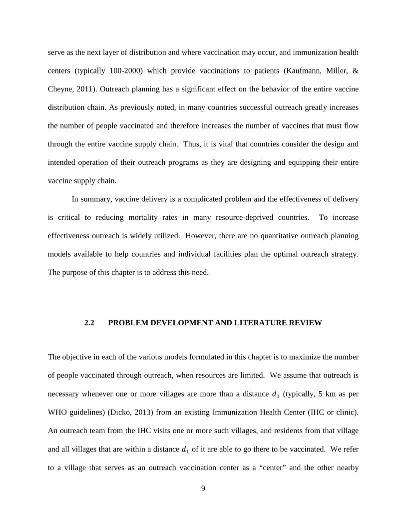
Figure 4. Coverage with first three models ................................................................................... 26

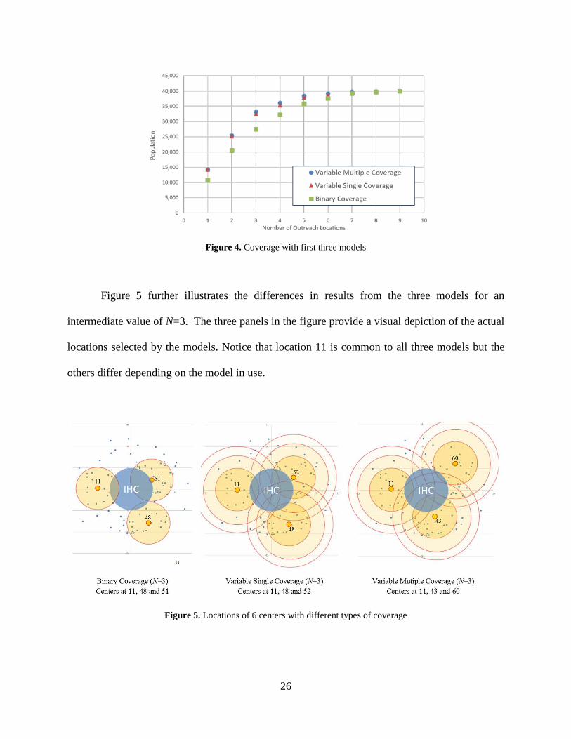
Figure 5. Locations of 6 centers with different types of coverage ................................................ 26

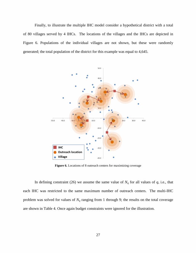
Figure 6. Locations of 8 outreach centers for maximizing coverage ............................................ 27

Figure 7. Packing arrangement in RCW25 for conventional inner packs (Top view) ................. 43

Figure 8. Packing arrangement in RCW25 for conventional inner packs with two additional inner packs ............................................................................................................................. 43

Figure 9. Packing configurations within inner packs for each proposed modular vial size ......... 48

Figure 10. Packing configurations within storage device ............................................................. 48

Figure 11. Tower packing method ................................................................................................ 50

Figure 12. Layer packing method ................................................................................................ 50

Figure 13. Signal Kanban example ............................................................................................... 71

Figure 14. Evolution strategy for the network problem .............................................................. 103

Figure 15. Chromosome examples ............................................................................................. 104

Figure 16. Crossover example .................................................................................................... 107

Figure 17. Example of handling a redundant hub in crossover .................................................. 108

xiii

Figure 18. Mutation .................................................................................................................... 109

Figure 19. Network graphs for Niger .......................................................................................... 112

Figure 20. ES results for Niger ................................................................................................... 114

Figure 21. Looping factor example ............................................................................................. 124

Figure 22. Apply looping factors ................................................................................................ 126

Figure 23. Network structure at each iteration (MIP-MIP) ........................................................ 131

Figure 24. Original ES vs Improved ES ..................................................................................... 133

xiv

ACKNOWLEDGEMENTS

First of all, I would like to thank my wife, Hyun Joo who sacrificed her career and was always

there for me caring and taking care of everything during my PhD studies. I could not finish my

dissertation without her support. I also want to thank my kids, Gahyun and Uijin. Your existence

has always encouraged me. I am indebted to my parents and parents-in-law for their endless

love, inspiration, encouragement and unconditional support. This dissertation is dedicated to my

family.

I would like to express my gratitude to my advisors, professors Bryan A. Norman and

Jayant Rajgopal, for guiding my dissertation research. Dr. Norman has given me the guideline to

pursue various areas and always has been patient to listen to new research topics. Dr. Rajgopal

has been supportive and has also provided intuitive discussions about the research. I am also very

grateful to Dr. Prokopyev for his recommendations and suggestions. Dr. Brown has supported

me by giving me valuable feedback on the dissertation.

Finally, I want to thank my friends and colleagues who have studied with me in the class

and office for my PhD life.

xv

1.0 INTRODUCTION

1.1 MOTIVATION AND RESEARCH OBJECTIVE

In 1974, the World Health Organization (WHO) established the Expanded Programme on

Immunization (EPI) to ensure that all children have access to vaccines recommended for routine

use (Bland & Clements, 1997). In many low and middle income countries, EPI and the Global

Alliance for Vaccines and Immunization (GAVI, which was established in 1999 to extend the

reach of EPI to the poorest countries) have combined to save millions of lives since the

establishment of these programs. According to 2013 WHO data (Immunization coverage, Fact

sheet N°378, 2014), world immunization coverage of diphtheria-tetanus-pertussis (DTP3), Polio,

Measles, Tetanus and Hepatitis B vaccines is over 80%. Yet, despite improvements in global

vaccine coverage during the past decade, there are millions of children in these countries who

still do not get the full regimen of childhood vaccines that are routinely given to children in the

developed world (GAVI, 2014) and limited resources, competing health priorities, poor

management of health systems, and inadequate monitoring and supervision remain as key

challenges. An estimated 22.8 million infants worldwide still miss getting basic vaccines.

There are a multitude of strategies that can be used to deliver immunization services and

there are two types of doses that can be given - routine or supplemental. The main distinction is

that a supplemental dose is “additional” or “extra” to the doses required by the national

1

immunization schedule and may, or may not, be recorded in the child's immunization record. On

the other hand, a routine dose is one that is prescribed according to the national immunization

schedule, is administered based on the vaccination history of each individual, counts towards

“fully immunized” status, and must be recorded on immunization cards and registers

(WHO/UNICEF Guidance Note, 2011).

By taking advantage of technology, low-cost mass production of many vaccines has

become possible. However, keeping vaccines available with low costs remains one of the major

challenges for vaccine supply chain managers. Most vaccines need to be maintained within a

narrow temperature range from the point of manufacture to their use in an immunization session,

within what is called the “cold chain,” which is essential to vaccine delivery. Many of the

challenges of getting vaccines to children result from the poor management or operation of the

vaccine supply chain. In particular, poor infrastructure and the constraints of the cold chain cause

inefficiency in vaccine storage and transportation (Zaffran, 1995, Yadav, Lydon, Oswald, Dicko,

& Zaffran, 2014).

In many low and middle income countries supported by EPI, vaccines are distributed via

their legacy medical supply chain, which is typically a three, four or five tier hierarchical

network. Vaccines are purchased by international organizations and delivered to a central

distribution center within each country from multiple suppliers/manufacturers. Through various

levels of the supply chain, vaccines are then delivered to clinics where the final recipients are

located. For example, Niger has a four-tier structure: central store, regional stores, district stores

and clinics. All vaccines come to the central store by air and are transported to children

successively through regional stores, district stores and finally, clinics. Figure 1 shows the health

facilities for Niger. Vaccines are periodically replenished at each facility in amounts that can

2

ensure adequate service until the next replenishment. In most countries, for locations that are not

conveniently located near a clinic, vaccination outreach activities are used, where health workers

visit such locations. Since each clinic has very limited resources, including health workers,

storage devices, transportation resources and time, teams from the clinic conduct outreach on

fixed days in selected locations by foot, or by using locally available means of transportation

(bicycles, locally arranged transport, etc.) (Ministry of Health, Government of Southern Sudan,

2009).

Figure 1. Health facilities for Niger

This study is motivated by the need to seek improvements in vaccine supply chains and

ultimately, to have more children be able to have access to vaccines via efficient network flow

and scientific management. It begins by studying the issue of outreach. Since outreach sessions

are usually not provided at the same location more than once a month and are planned and

3

organized with the community, they should be arranged such that they cover as many children as

possible during the limited number of sessions. This study introduces several vaccine outreach

models with different assumptions based on the maximal coverage location problem and

investigates the results.

The second focus of this research is on certain logistics aspects of vaccine delivery.

Specifically it examines issues associated with storing vaccines efficiently in a storage device

when transporting them, and on handling the replenishment process at facilities. When an upper

level distribution center or hospital prepares the vaccines to send to lower level distribution

centers or clinics, they are often sent in inner packs, which constitute a secondary packaging

mode for vaccines. These inner packs are the units in which vials are stored within larger cartons

and because of their irregular sizes they can lead to inefficient space utilization within a storage

device. This study is designated to clarify the benefits of the modular vaccine packaging which is

proposed in Chapter 3. In related work, a vaccine ordering policy is also studied. Currently, at a

clinic where actual vaccination occurs the vaccines are ordered in vial units. However, counting

several kinds of vaccine vials and ordering them can lead to errors in the ordering process and

increases ordering and order fulfillment effort. An ordering policy that is based on using inner

pack quantities is proposed that can reduce ordering errors and order fulfillment effort.

In the third part of this research, the problem of redesigning a whole vaccine supply chain

is studied. Currently, in many countries vaccines are distributed via their legacy medical supply

chain which is typically not cost-efficient. Because vaccines require a cold supply chain,

capacity constraints on cold storage and cold transport are critical. Redesigning the vaccine

supply chain includes: choosing intermediate hubs among the current distribution center

locations, determining the flow paths from the central distribution facility (where vaccines are

4

received into a country) to health clinics where vaccination actually occurs, the transportation

vehicles to allocate to each flow path, and storage devices to use at each location. The re-

designed network does not have to follow the current three or four tiered strictly arborescent

structure commonly found in practice but can use alternative network structures. To re-design

this network, we develop a mixed-integer optimization model and also suggest heuristic methods

to get an approximate solution for larger problems. Numerical results are presented using real

data from different countries.

1.2 CONTRIBUTIONS

This dissertation develops models for analyzing the issues raised above. The major contributions

are:

• The formulation and solution of mixed integer programming (MIP) models for vaccine

outreach at the clinic level.

• Robustness analysis on outreach MIP models with respect to uncertain demand in outreach

locations and uncertain coverage assumptions.

• Development of a spreadsheet model that evaluates the impact of different modular packing

schemes and uses data from the Benin and Niger routine regimen along with commonly

used vaccine carriers.

• Applying lean concepts that have been used in the manufacturing sector to vaccine inventory

management, in order to simplify ordering procedures and evaluate the impact on storage

and transportation resources.

5

• Creation of a MIP model for redesigning the WHO-EPI vaccine distribution chain in any

country and developing a hybrid evolutionary strategy /MIP algorithm to solve the model.

• Development on an algorithm to apply vehicle routing strategies to a vaccine distribution

network.

6

2.0 COVERAGE MODELS TO DETERMINE OUTREACH VACCINATION

CENTER LOCATIONS IN LOW AND MIDDLE INCOME COUNTRIES

2.1 INTRODUCTION

Vaccine delivery in many low and middle income countries is an extremely complex problem.

The supply chains in such countries are limited in their cold-storage capacity and in their ability

to transport vaccines quickly to various points throughout the country. In addition to these

supply chain limitations, most of these countries have geographically dispersed or nomadic

populations. Portions of their populations have limited or no access to vaccination locations due

to poor infrastructure (poor road conditions or limited transportation) or other geographic

barriers. As examples, in the country of Niger, 90% of the roads are unpaved (Blanford, Kumar,

Luo, & MacEachren, 2012). In Nigeria, people from some rural areas may have to walk at least

26 miles to access health care (BBC, 2006). In Kenya, 40% of the population must travel in

excess of an hour to the nearest primary healthcare facility (Noor, Amin, Gething, Atkinson,

Hay, & Snow, 2006). Thus, people from remote locations within resource-deprived countries

have difficulty reaching immunization locations for their standard regimen of vaccines. This puts

these individuals at a very high risk of mortality from infectious diseases such as measles, yellow

fever, polio and tuberculosis.

7

One method to overcome this challenge is to use outreach. Sustained outreach is a

strategy for reaching remote sections of the population with limited access to immunization

locations. With this service, health care workers take vaccines from a fixed immunization

location and travel to the remote locations, to immunize individuals there. This service is

different from a campaign which is a one-time attempt to raise immunization rates. Outreach is

extremely important to the overall immunization programs in resource-deprived countries.

Without outreach, many countries would suffer from extremely low coverage rates. For

example, a study was carried out in three zones of different population densities within Kenya to

test the effectiveness of outreach programs as compared to only utilizing fixed immunization

locations. The study showed that with outreach, the coverage rate increased from 25% to 57% in

the zone with lowest population density. Coverage increased from 54% to 82% in the zone with

greatest population density (World Health Organization, 1997).

Outreach is typically provided on a systematic basis, at regular time intervals and regular

outreach locations. However, the outreach activities conducted from each immunization location

can vary greatly depending on financial resources, time constraints, vaccine availability,

population characteristics, usage rate of the fixed immunization location, health worker training,

portable cold chain equipment available, and transportation available. The decisions about when

and where to conduct outreach and which vaccines to administer, are often made locally,

depending on each location’s available resources (World Health Organization, 2001).

Outreach from health centers constitutes the critical final link in the vaccine supply chain,

which can be quite complex and is typically comprised of four levels in addition to outreach: a

central location where vaccines are received into the country from manufacturers, regional

locations (typically five to 10) that serve as distribution hubs, districts (typically 25-100) which

8

serve as the next layer of distribution and where vaccination may occur, and immunization health

centers (typically 100-2000) which provide vaccinations to patients (Kaufmann, Miller, &

Cheyne, 2011). Outreach planning has a significant effect on the behavior of the entire vaccine

distribution chain. As previously noted, in many countries successful outreach greatly increases

the number of people vaccinated and therefore increases the number of vaccines that must flow

through the entire vaccine supply chain. Thus, it is vital that countries consider the design and

intended operation of their outreach programs as they are designing and equipping their entire

vaccine supply chain.

In summary, vaccine delivery is a complicated problem and the effectiveness of delivery

is critical to reducing mortality rates in many resource-deprived countries. To increase

effectiveness outreach is widely utilized. However, there are no quantitative outreach planning

models available to help countries and individual facilities plan the optimal outreach strategy.

The purpose of this chapter is to address this need.

2.2 PROBLEM DEVELOPMENT AND LITERATURE REVIEW

The objective in each of the various models formulated in this chapter is to maximize the number

of people vaccinated through outreach, when resources are limited. We assume that outreach is

necessary whenever one or more villages are more than a distance 𝑑𝑑1 (typically, 5 km as per

WHO guidelines) (Dicko, 2013) from an existing Immunization Health Center (IHC or clinic).

An outreach team from the IHC visits one or more such villages, and residents from that village

and all villages that are within a distance 𝑑𝑑1 of it are able to go there to be vaccinated. We refer

to a village that serves as an outreach vaccination center as a “center” and the other nearby

9

villages (within distance 𝑑𝑑1) from which residents travel to the center as “satellite” villages. The

maximum number of centers that can be selected for outreach during the planning horizon

depends on the financial and other resources available at the IHC. The objective is to select

centers so as to maximize the number of residents that can be served at each of the central

villages and its respective satellite villages.

As an illustrative example, Figure 2 shows seven villages (represented by the small

circles) located near an IHC along with their corresponding patient populations (represented by

the numbers above the circles). Three options are shown for the selection of an outreach center

from that IHC. If village A is selected as the center [Case A], then the satellite villages that are

within 5 km are villages B, C, and D, and thus people in villages A, B, C and D can be

vaccinated. People in villages E, F and G will not be vaccinated. In this case, the number of

residents that can be covered by outreach is 170. Similarly, 180 people can be covered in Case

B and 160 in Case C. Therefore, if we are restricted to a single outreach location, then among

these three villages, B would be the best option for a center.

[Case A] [Case B] [Case C]

Figure 2. Outreach example: selecting an outreach location

10

While more than one outreach strategy might be possible, there will typically be

constraints that limit the final choice of outreach options. For example, outreach to a particular

location has a cost associated with it (that might depend upon distance or terrain or equipment

used) and there might be some overall budget for outreach that constrains our choice of outreach

trips. Alternatively, costs might be similar for outreach to different sites but we might have a

direct limit on the number of outreach sessions (e.g., because of personnel, vehicle, or equipment

limits). In other cases, there might be limits on the length of a trip or preferences for certain trips

over others. Different strategies are possible depending on these constraints and the assumptions

made on the type and amount of patient coverage that can be obtained at a center.

In this chapter, we introduce three models that have different coverage assumptions and

an integrated model for multiple IHCs. In addition, we consider the robustness of our solutions

with respect to coverage assumptions and uncertainty in demand.

Daskin and Dean (2004) discuss how the location set covering model, maximal covering

model and P-median model have been used for location planning in health care and review other

models derived from these three basic facility models. The different model types are applied

selectively according to a problem's characteristics and objective. The problem addressed here

may be viewed as a covering problem, which is well-known among facility location models

(Farahani, Asgari, Heidari, Hosseininia, & Goh, 2012). In particular, it is related to the Maximal

Covering Location Problem (MCLP), which was developed by Church and ReVelle (Church &

ReVelle, 1974), with the objective of maximizing the amount of demand covered by a facility. In

this model, it is assumed that all demand is covered if the demand location is within an

acceptable service distance, otherwise it is not, i.e., coverage is binary. An extension to this is the

concept of partial coverage, in which there are two distances: the maximum full coverage

11

distance D1 and the minimum non-coverage distance D2. The demand within distance D1 from a

facility is fully covered while none of the demand beyond distance D2 is covered. For demand at

locations between distances D1 and D2 from the facility, the coverage level is assumed to be a

decreasing function of the distance to the demand location. Thus, some customers are fully

covered and the others are partially covered (Berman & Krass, 2002). This variation has been

called the gradual covering problem by Drezner, Wesolowsky, and Drezner (2004), or MCLP

with partial coverage by Karasakal and Karasakal (2004). Berman and Krass (2002) collectively

refer to this class of models as the Generalized Maximal Covering Location Problem (GMCLP).

In order to apply linear programming, they assume that the function for partial coverage is

stepwise decreasing, so that the model is similar to MCLP. In these models, all demand at a

location is assigned to the nearest facility, even though there might be two or more facilities near

the demand location that are capable of serving the demand. Berman, Drezner, and Krass (2009)

introduce the cooperative coverage model where the effect of facilities is combined if there are

more than two facilities near the demand location. However, in this model the coverage is once

again binary, with a demand location being fully covered if an aggregation of partial coverage

possible from nearby facilities exceeds a certain threshold; otherwise there is no coverage. That

is, there is no partial coverage of demand points.

2.3 COVERAGE MODELS

In this section, we consider four types of models to optimize coverage from outreach. In all of

our models we consider multiple outreach locations that can be selected. We start with a basic

model that is similar to the binary MCLP model. The second model extends this by drawing

12

from the GMCLP approach, with coverage being a stepwise and decreasing function of distance.

The third model is a new generalization of the cooperative cover model: rather than being binary,

an accumulation of partial coverage becomes the partial coverage of the location. The final

model is a larger one that could be viewed as a generalization of any of the first three models.

Here we formulate it as an extension of the second one, where each facility is constrained to lie

within a given radial distance from one of several specific points (the IHCs).

For ease of exposition, we assume that there is sufficient capacity to vaccinate the people

who are targeted by an outreach trip (although it would be a straightforward extension to add in

capacity constraints for trips). These models are described in the next four subsections, followed

by numerical illustrations of each in the section after that. The illustrations use data that is

generated from partial information on the state of Bihar in northern India that was obtainable,

and which was the motivating application for this work. We conclude with a discussion and

summary of our work in the final section.

2.3.1 Model 1: Binary coverage model

In this basic model, it is assumed that residents in villages within a radius of 𝐷𝐷1 km from an

outreach center are covered, while residents in other villages are not.

Notation:

𝑛𝑛: Total number of villages to be served via outreach from the IHC

𝑝𝑝𝑖𝑖: Number of residents living in village 𝑖𝑖

𝑐𝑐𝑖𝑖: Cost of outreach at village 𝑖𝑖 if it serves as an outreach center

𝑑𝑑𝑖𝑖𝑖𝑖: Distance between village 𝑖𝑖 and village 𝑗𝑗 (with 𝑑𝑑𝑖𝑖𝑖𝑖 = 0)

𝐷𝐷1: Maximal coverage distance

13

𝐶𝐶: Available budget for outreach

𝑁𝑁: Maximum number of outreach centers that is feasible

𝑥𝑥𝑖𝑖∈{0, 1}: 1 if village 𝑖𝑖 is selected as an outreach center; 0 otherwise

𝑦𝑦𝑖𝑖∈{0, 1}: 1 if village 𝑖𝑖 is covered; 0 otherwise

The mathematical model is as follows:

𝑀𝑀𝑀𝑀𝑥𝑥 �𝑝𝑝𝑖𝑖𝑦𝑦𝑖𝑖

𝑛𝑛

𝑖𝑖=1

(1)

subject to

𝑦𝑦𝑖𝑖 ≤ � 𝑥𝑥𝑖𝑖𝑖𝑖∈𝑆𝑆𝑖𝑖

for 𝑆𝑆𝑖𝑖 = �𝑗𝑗:𝑑𝑑𝑖𝑖𝑖𝑖 ≤ 𝐷𝐷1, 𝑗𝑗 = 1, … ,𝑛𝑛�, 𝑖𝑖 = 1, … ,𝑛𝑛 (2)

�𝑐𝑐𝑖𝑖𝑥𝑥𝑖𝑖

𝑛𝑛

𝑖𝑖=1

≤ 𝐶𝐶 (3)

�𝑥𝑥𝑖𝑖

𝑛𝑛

𝑖𝑖=1

≤ 𝑁𝑁 (4)

𝑥𝑥𝑖𝑖∈{0,1}, 𝑦𝑦𝑖𝑖∈{0,1}, for 𝑖𝑖 = 1, … ,𝑛𝑛 (5)

The objective is to maximize the number of people who are vaccinated by outreach

(across all villages selected along with their respective satellites). Constraint (2) ensures that

village i is covered only if it is D1 km or less from any village j which serves as an outreach

center (a typical value for D1 might be 5 km). Constraints (3) and (4) respectively ensure that the

available outreach budget and the limit on the number of outreach centers are not exceeded. It is

conceivable that only one of these constraints might exist.

14

2.3.2 Model 2: Variable single coverage model

In this model, it is assumed that the coverage by outreach is a stepwise decreasing function of

distance from an outreach center, rather than being binary. Given D1<D2<…<DK and

1=α1>α2>…>αK>0, coverage is divided into groups:

• If there are centers within distance D1 of the village, all residents (i.e., a fraction α1=1) go to

one such center; else

• If there are centers between distance D1 and D2, then a fraction α2 of the patient population

will choose to visit one such center; else

• …

• If there are centers between distance DK-1 and DK, then a fraction αK of the population will

choose to visit one such center; else

• There is no coverage.

A typical example might be K=3 with D1=5 km, D2=8 km, D3=10 km, and α1=1, α2=0.5,

α3=0.2.

Additional notation is as follows:

𝐷𝐷𝑘𝑘: Distance from the outreach center of the 𝑘𝑘𝑡𝑡ℎ coverage boundary,𝑘𝑘 = 1,2, … ,𝐾𝐾

𝛼𝛼𝑘𝑘: Coverage fraction attained if the nearest center is between 𝐷𝐷𝑘𝑘−1 and 𝐷𝐷𝑘𝑘 𝑘𝑘𝑘𝑘 of 𝑀𝑀 village

Instead of the yi variables of the prior section we now have

𝑦𝑦𝑖𝑖𝑘𝑘 ∈ {0, 1}: 1 if village i is covered by a center between 𝐷𝐷𝑘𝑘−1 and 𝐷𝐷𝑘𝑘 𝑘𝑘𝑘𝑘 of it; 0 otherwise

The model is as follows:

𝑀𝑀𝑀𝑀𝑥𝑥 �𝑝𝑝𝑖𝑖�𝛼𝛼𝑘𝑘𝑦𝑦𝑖𝑖𝑘𝑘

𝐾𝐾

𝑘𝑘=1

𝑛𝑛

𝑖𝑖=1

(6)

subject to

15

𝑦𝑦𝑖𝑖𝑘𝑘 ≤ � 𝑥𝑥𝑖𝑖

𝑖𝑖∈𝑆𝑆𝑖𝑖

𝑓𝑓𝑓𝑓𝑓𝑓 𝑆𝑆𝑖𝑖 = �𝑗𝑗:𝐷𝐷𝑘𝑘−1 ≤ 𝑑𝑑𝑖𝑖𝑖𝑖 ≤ 𝐷𝐷𝑘𝑘, 𝑗𝑗 = 1, … ,𝑛𝑛�, 𝑖𝑖 = 1, … , 𝑛𝑛;

𝑘𝑘 = 1, … ,𝐾𝐾

(7)

�𝑦𝑦𝑖𝑖𝑘𝑘

𝐾𝐾

𝑘𝑘=1

≤ 1 𝑓𝑓𝑓𝑓𝑓𝑓 𝑖𝑖 = 1, … ,𝑛𝑛 (8)


𝑛𝑛

𝑖𝑖=1

≤ 𝐶𝐶 (9)

�𝑥𝑥𝑖𝑖

𝑛𝑛

𝑖𝑖=1

≤ 𝑁𝑁 (10)

𝑥𝑥𝑖𝑖∈{0,1}, 𝑦𝑦𝑖𝑖𝑘𝑘∈{0,1}, 𝑓𝑓𝑓𝑓𝑓𝑓 𝑖𝑖 = 1, … ,𝑛𝑛, 𝑘𝑘 = 1, … ,𝐾𝐾 (11)

In this model the objective is the same as in the previous model but coverage is according

to the appropriate coverage fraction. Constraint (7) ensures that yik can be 1 only if village i is

within the appropriate coverage radius from any outreach center. Constraint (8) ensures that

village i is assigned to at most one outreach center. Constraints (9) and (10) are the usual

budget/resource constraints akin to (3) and (4) in Model 1.

2.3.3 Model 3: Variable multiple coverage model

The third model is a generalization of the second one: villages that are not within the 100%

coverage distance D1 are not restricted to partial coverage by a single center (unless it is the only

available choice). Rather, residents who do not visit one such center might choose to visit

another one. More specifically, given D1<D2<…<DK and 1=α1>α2>…>αK>0, coverage follows

the following pattern:

• If there are m1>0 centers within distance D1 of the village, all residents (i.e., a fraction α1=1)

go to one such center; else

16

• If there are m2>0 centers between distance D1 and D2, then a fraction α2 of the population will

choose to visit one such center; a further fraction α2 of the remaining population will choose

to visit another such center; and so on

…

• If there are mK>0 centers between distance DK-1 and DK, then a fraction αK of the remaining

population will choose to visit one such center; a further fraction αK of the remaining

population will choose to visit another such center; and so on

• There is no coverage if there is no center within distance DK of the village

In general, the coverage in a village would be given by

𝛽𝛽 = 1 −�(1 − 𝛼𝛼𝑘𝑘)𝑚𝑚𝑘𝑘

𝐾𝐾

𝑘𝑘=2

As an example, with K=3, D1=5 km, D2=8 km, D3=10 km, α1=1, α2=0.5, α3=0.2, m1=0,

m2=2, m3=1, the fraction of residents covered would be given by 1-(1-0.5)2(1-0.2)1 = 0.80. Thus,

if the village had 100 residents, since there are no centers in the inner circle, 50% (i.e., 50) would

go to one of the two centers in the next circle while 50% of the remaining 50 (i.e., 25) would go

to the other, and 20% of the remaining 25 (i.e., 5) would go to the center in the outer circle; 20

residents would choose not to go to any center for immunization. To further illustrate the

difference between the model in this section and the previous one, consider the Figure 3 with

four outreach centers in a region of 20 villages; these centers are located at villages 2, 8, 10 and

14. Suppose that as before α1=1, α2=0.5 and α3=0.2 in both models.

17

Figure 3. Variable outreach coverage example

Consider village 6 and 11, neither of which is within the inner circle of any center and

thus cannot receive 100% coverage. Village 6 is within the outer circles of centers located at

villages 8 and 10: with Model 2, the coverage would be 20%, all at one of centers 8 or 10. With

Model 3, the coverage would be 36%: 20% at one of 8 or 10, and 16% (i.e., 20% of the

remaining 80%) at the other. Village 11 is within the middle circle of the centers at locations 10

and 14 and within the outer circle of the center at location 8. Here the coverage would be 50%

with the first model (at either center 10 or center 14), but in the second model with three possible

center options, it would be 1-(1-0.5)2(1-0.2)=80% (50% at one of villages 10 and 14 and 25% at

the other, 5% at village 8).

In our formulation of this problem we restrict ourselves to K=3. Define the following

additional notation:

𝑀𝑀𝑟𝑟: Maximum number of villages within the 𝑓𝑓𝑡𝑡ℎ coverage circle of any village, 𝑓𝑓 = 1,2,3

𝛽𝛽𝑚𝑚2𝑚𝑚3: Coverage constant with 𝑘𝑘2 centers between (𝐷𝐷1,𝐷𝐷2) and 𝑘𝑘3 centers between (𝐷𝐷2,𝐷𝐷3) = 1 − (1 − 𝛼𝛼2)𝑚𝑚2(1 − 𝛼𝛼3)𝑚𝑚3

𝑧𝑧𝑖𝑖𝑘𝑘𝑖𝑖 ∈ {0, 1}: 1 if there are no centers located within distance 𝐷𝐷1of 𝑖𝑖,𝑘𝑘 centers located between

distance (𝐷𝐷1,𝐷𝐷2) of 𝑖𝑖, and 𝑙𝑙 centers located between distance (𝐷𝐷2,𝐷𝐷3) of village 𝑖𝑖; 0 otherwise

1

3 4 5

6

7 8

2

9

10

11

14

12

15 16

13 19

18 17

20

18

Instead of the yik variables of the prior section we now have

𝑦𝑦𝑖𝑖 ∈ {0, 1}: 1 if there is at least one center located within distance 𝐷𝐷1of 𝑖𝑖; 0 otherwise

The values of 𝑀𝑀𝑟𝑟 are determined a priori by preprocessing. To illustrate the notation,

consider the outreach assignment shown in Figure 2-2. For village 11, we have 0 centers within

distance D1, 2 centers between distance (D1, D2), and 1 center between distance (D2, D3). Thus

z11,2,1=1 and z11,k,l=0 for all other k, l. For village 19, the corresponding numbers are 1, 0, and 2,

but the model will insure z19,k,l=0 for all k, l because there is a center located within distance D1

of village 19.


𝑀𝑀𝑀𝑀𝑥𝑥 �𝑝𝑝𝑖𝑖𝑦𝑦𝑖𝑖

𝑛𝑛

𝑖𝑖=1

+ ��𝑝𝑝𝑖𝑖𝛽𝛽𝑘𝑘𝑖𝑖𝑧𝑧𝑖𝑖𝑘𝑘𝑖𝑖

𝑀𝑀3

𝑖𝑖=0

𝑀𝑀2

𝑘𝑘=0

𝑛𝑛

𝑖𝑖=1

(12)

subject to


𝑓𝑓𝑓𝑓𝑓𝑓 𝑆𝑆𝑖𝑖 = �𝑗𝑗:𝑑𝑑𝑖𝑖𝑖𝑖 ≤ 𝐷𝐷1, 𝑗𝑗 = 1, … ,𝑛𝑛�, 𝑖𝑖 = 1, … ,𝑛𝑛 (13)

�� 𝑧𝑧𝑖𝑖𝑘𝑘𝑖𝑖

𝑀𝑀3

𝑖𝑖=0

𝑀𝑀2

𝑘𝑘=0

+ 𝑦𝑦𝑖𝑖 ≤ 1 (14)

�𝑘𝑘�𝑧𝑧𝑖𝑖𝑘𝑘𝑖𝑖

𝑀𝑀3

𝑖𝑖=0

𝑀𝑀2

𝑘𝑘=0

≤ � 𝑥𝑥𝑖𝑖𝑖𝑖∈𝑆𝑆𝑖𝑖

𝑓𝑓𝑓𝑓𝑓𝑓 𝑆𝑆𝑖𝑖 = �𝑗𝑗:𝐷𝐷1 < 𝑑𝑑𝑖𝑖𝑖𝑖 ≤ 𝐷𝐷2, 𝑗𝑗 = 1, … ,𝑛𝑛�, 𝑖𝑖 = 1, … ,𝑛𝑛 (15)

�𝑙𝑙�𝑧𝑧𝑖𝑖𝑘𝑘𝑖𝑖

𝑀𝑀2

𝑘𝑘=0

𝑀𝑀3

𝑖𝑖=0


𝑓𝑓𝑓𝑓𝑓𝑓 𝑆𝑆𝑖𝑖 = �𝑗𝑗:𝐷𝐷2 < 𝑑𝑑𝑖𝑖𝑖𝑖 ≤ 𝐷𝐷3, 𝑗𝑗 = 1, … , 𝑛𝑛�, 𝑖𝑖 = 1, … ,𝑛𝑛 (16)


𝑛𝑛

𝑖𝑖=1

≤ 𝐶𝐶 (17)

�𝑥𝑥𝑖𝑖

𝑛𝑛

𝑖𝑖=1

≤ 𝑁𝑁 (18)

𝑥𝑥𝑖𝑖∈{0,1}, 𝑦𝑦𝑖𝑖∈{0,1}, 𝑓𝑓𝑓𝑓𝑓𝑓 𝑖𝑖 = 1, … ,𝑛𝑛 (19)

𝑧𝑧𝑖𝑖𝑘𝑘𝑖𝑖∈{0,1}, 𝑓𝑓𝑓𝑓𝑓𝑓 𝑖𝑖 = 1, … ,𝑛𝑛 , 𝑘𝑘 = 0, … ,𝑀𝑀2, 𝑙𝑙 = 0, … ,𝑀𝑀3 (20)

19

The objective in this model has two terms: the first one counts the number of residents in

villages with 100% coverage and the second in villages that obtain partial coverage. Constraints

(14), (18) and (19) are similar to the ones in the prior models, while (15) ensures that if village i

gets coverage, it is either 100% coverage or partial coverage from one particular combination of

villages in the inner and outer secondary coverage circles. Constraints (16) and (17) along with

the fact that βkl is monotone increasing in k and l ensure that zikl =1 when there are k centers

located between distance (D1,D2) and l centers located between distance (D2,D3) of village i.

2.3.4 Model 4: Model with multiple IHCs

In the last model we consider an entire district with multiple IHCs located within it. It is

possible that a particular village might be a candidate for outreach from more than one IHC. This

model addresses the problem of developing the best combination of outreach programs across all

IHCs within a district. We could embed any of the models of the previous section into a larger

problem for the entire district as appropriate; here we illustrate the model using the case where

there is variable single coverage at each village (as in Model 2). Additional notation is as

follows:

𝑘𝑘: Number of different IHCs in the district

𝑁𝑁𝑞𝑞: Maximum number of outreach activities from IHC 𝑞𝑞

𝐷𝐷𝑚𝑚𝑚𝑚𝑚𝑚: Maximum travel distance to an outreach location from any IHC

We define yik similar to what we did in the variable single coverage model but also define

𝑥𝑥𝑖𝑖𝑖𝑖 = {0, 1}: 1 if village i is selected as a center for outreach from IHC 𝑙𝑙; 0 otherwise

20


𝑀𝑀𝑀𝑀𝑥𝑥 �𝑝𝑝𝑖𝑖�𝛼𝛼𝑘𝑘𝑦𝑦𝑖𝑖𝑘𝑘

𝐾𝐾

𝑘𝑘=1

𝑛𝑛

𝑖𝑖=1

(21)

subject to

𝑦𝑦𝑖𝑖𝑘𝑘 ≤ ��𝑥𝑥𝑖𝑖𝑖𝑖

𝑚𝑚

𝑞𝑞=1𝑖𝑖∈𝑆𝑆𝑖𝑖

𝑓𝑓𝑓𝑓𝑓𝑓 𝑆𝑆𝑖𝑖 = �𝑗𝑗:𝐷𝐷𝑘𝑘−1 ≤ 𝑑𝑑𝑖𝑖𝑖𝑖 ≤ 𝐷𝐷𝑘𝑘, 𝑗𝑗 = 1, … ,𝑛𝑛�,

𝑖𝑖 = 1 𝑡𝑡𝑓𝑓 𝑛𝑛 , 𝑘𝑘 = 1, … ,𝐾𝐾

(22)


𝐾𝐾

𝑘𝑘=1

≤ 1 𝑓𝑓𝑓𝑓𝑓𝑓 𝑖𝑖 = 1, … ,𝑛𝑛 (23)


𝑛𝑛

𝑖𝑖=1

≤ 𝐶𝐶 (24)

�𝑥𝑥𝑞𝑞𝑖𝑖

𝑛𝑛

𝑖𝑖=1

≤ 𝑁𝑁𝑞𝑞 𝑓𝑓𝑓𝑓𝑓𝑓 𝑞𝑞 = 1, … ,𝑘𝑘 (25)

𝑑𝑑𝑞𝑞𝑖𝑖𝑥𝑥𝑞𝑞𝑖𝑖 ≤ 𝐷𝐷𝑚𝑚𝑚𝑚𝑚𝑚 𝑓𝑓𝑓𝑓𝑓𝑓 𝑞𝑞 = 1, … ,𝑘𝑘, 𝑗𝑗 = 1, … ,𝑛𝑛 (26)

�𝑥𝑥𝑞𝑞𝑖𝑖

𝑚𝑚

𝑞𝑞=1

≤ 1 𝑓𝑓𝑓𝑓𝑓𝑓 𝑖𝑖 = 1, … ,𝑛𝑛 (27)

𝑥𝑥𝑞𝑞𝑖𝑖∈{0,1}, 𝑦𝑦𝑖𝑖𝑘𝑘∈{0,1}, 𝑓𝑓𝑓𝑓𝑓𝑓 𝑖𝑖 = 1, … ,𝑛𝑛, 𝑘𝑘 = 1, … ,𝐾𝐾; 𝑞𝑞 = 1, … ,𝑘𝑘 (28)

Here C represents the budget for the entire district in (25), a separate limit on the number

of outreach sessions is defined for each IHC along with a distance constraint for each IHC in

(26) and (27), and (28) that ensures that if there is an outreach center at a village it must come

from a unique IHC.

2.3.5 Numerical example

We first illustrate the binary, variable single and multiple coverage models with the following

example based on the Tetia Bambar IHC in the state of Bihar, India. This IHC has a total of 92

21

villages in its catchment area that are candidates for outreach centers. We were provided with the

distances from the IHC to each outreach village and the patient populations at each village.

However, the exact locations of these villages in relation to Tetia Bambar were not available, and

given their small sizes and inconsistencies in how their names were spelled it was impossible to

accurately locate them on any map. We therefore located the IHC at (0, 0) and randomly

assigned coordinates to the villages while maintaining the given distances. The resulting

coordinates of the villages along with their patient populations are listed in Table 1.

We use coordinate units of 1 km and assume that all distances dij are Euclidean. For the

binary coverage model we assume D1 = 5 km. For the variable coverage models, we also assume

D2 = 8 km and D3 = 10 km along with coverage fractions α2= 0.5 and α3= 0.2. In order to

compare the results across the various models we ignored the budget constraints (i.e., (3), (9),

and (17)) because it was impossible to obtain even approximate estimates from Bihar. We only

used the constraints on the maximum number of outreach activities (centers), N (i.e., (4), (10),

and (18)). We solved each model for increasing values of N until we obtained 100% coverage.

For each model, Table 2 lists the coverage obtained for each value of N, along with the

respective locations of the outreach centers. The numbers in bold face represent new locations of

outreach centers that are added to or replace the ones from the previous (lower) value of N.

The three models often give different locations and levels of coverage when the limit on

the number of centers does not allow for 100% coverage. As an example when only 4 centers

are possible the coverage is 80.9% with Model 1, 88.6% with Model 2 and 90.5% with Model 3,

and the models do not select the same 4 locations. However, as the number of possible centers

(and the corresponding coverage) increases the centers start to converge to the same locations.

In all cases, a total of 9 centers are required before 100% coverage can be obtained; the locations

22

are identical and such that each village is within the inner circle (5 km radius) of at least one

center. Another interesting observation is that while one new center is always added as we

increase N, there are many instances with all models where in addition to adding a new center an

existing location is replaced with a new one. This emphasizes the value of an optimization model

in selecting the best strategy. As an example, with Models 1 and 2, when N changes from 7 to 8

four of the existing centers are replaced with five new ones; there are only three in common.

Similarly, with Models 2 and 3, when N changes from 2 to 3, the two existing locations are

replaced by three completely new ones.

Table 1. Location information

Village Location Population Village Location Population X Y X Y 1 -11.84 4.93 228 47 1.38 -9.63 525 2 -11.03 -7.51 646 48 1.49 5.38 348 3 -10.07 2.85 366 49 1.53 10.24 401 4 -10.07 3.61 671 50 1.84 5.19 706 5 -9.88 0.40 594 51 1.94 4.89 650 6 -9.78 -3.48 624 52 1.97 -5.86 865 7 -8.93 3.79 711 53 2.76 -9.79 624 8 -8.88 2.25 475 54 2.85 3.49 44 9 -7.95 -3.40 198 55 2.92 2.91 147

10 -7.75 -6.21 561 56 3.05 -2.49 563 11 -7.52 0.19 525 57 3.18 5.46 273 12 -7.13 6.73 1,049 58 3.39 -9.66 618 13 -6.25 -2.92 554 59 3.43 -4.51 748 14 -6.07 0.06 496 60 3.96 -7.97 756 15 -5.37 -1.48 701 61 3.97 0.59 508 16 -5.19 3.30 293 62 4.59 -7.89 348 17 -5.14 -5.06 955 63 4.63 1.50 541 18 -4.67 -8.98 466 64 4.65 4.82 240 19 -4.65 11.30 246 65 4.69 2.13 463 20 -4.54 8.41 203 66 5.08 2.93 434 21 -4.38 2.98 297 67 5.29 -2.83 413 22 -4.14 -3.25 398 68 5.59 9.87 848 23 -3.67 0.41 695 69 5.61 -0.88 584 24 -3.60 9.14 254 70 5.76 -5.74 661 25 -3.48 -1.44 160 71 6.00 -0.57 636 26 -3.23 0.92 498 72 6.60 -0.74 682 27 -2.78 -3.86 442 73 6.71 -8.85 646 28 -2.62 -9.70 317 74 6.72 5.99 485 29 -2.38 -6.37 281 75 6.78 -7.45 541 30 -2.36 -2.23 278 76 7.12 1.47 792

23

Table 1 (continued) 31 -1.74 -8.48 736 77 7.32 0.80 592 32 -1.65 -7.33 566 78 7.47 8.17 573 33 -0.96 3.30 387 79 7.48 6.37 423 34 -0.89 -10.30 195 80 7.70 5.60 493 35 -0.78 -3.81 743 81 7.73 1.48 694 36 -0.71 -3.05 370 82 7.82 -7.71 470 37 -0.62 11.76 553 83 8.05 -6.30 482 38 -0.41 -7.66 272 84 8.14 -1.24 355 39 -0.14 8.26 627 85 8.90 3.83 692 40 0.08 -10.23 543 86 8.94 3.94 677 41 0.24 -8.79 473 87 9.03 0.51 540 42 0.31 -9.84 329 88 9.53 3.62 90 43 0.41 -7.65 374 89 10.03 5.38 613 44 0.62 -10.20 491 90 10.27 6.24 313 45 1.11 6.30 392 91 12.16 -4.61 488 46 1.19 3.24 619 92 12.88 1.33 456

Table 2. Results for the first three models

Model 1: Binary Coverage Model 2: Variable single coverage

Model 3: Variable multiple coverage

N No. Covered

Percent Covered

Center Locations

No. Covered

Percent Covered

Center Locations

No. Covered

Percent Covered

Center Locations

1 10,749 26.9% 51 14,238 35.7% 53 14,238 35.7% 53

2 20,515 51.4% 48, 51 25,167 63.1% 30, 51 25,463 63.8% 30, 51

3 27,417 68.7% 11, 48, 51 32,390 81.2% 11, 48, 52 33,093 83.0% 11, 43, 60

4 32,257 80.9% 8, 17, 48, 51 35,331 88.6% 7, 17, 48,

52 36,119 90.5% 5, 31, 35, 62

5 35,812 89.8% 8, 17, 31, 48, 62 37,853 94.9% 8, 17, 31,

48, 62 38,347 96.1% 8, 17, 31, 48, 62

6 37,590 94.2% 8, 17, 31, 48, 60, 73 38,742 97.1% 8, 17, 31,

48, 60, 73 39,132 98.1% 8, 17, 31, 48, 60, 73

7 39,259 98.4% 6, 8, 30, 31, 60, 69 ,73 39,572 99.2%

6, 8, 30, 31, 60, 69, 73

39,746 99.6% 6, 8, 30, 31, 60, 69, 73

8 39,666 99.4% 10, 11, 23, 35, 39, 60, 69, 73

39,780 99.7% 10, 11, 23, 35, 39, 60, 69, 73

39,844 99.9% 6, 8, 23, 30, 39, 60, 69, 73

9 39,894 100.0% 8, 10, 22, 23, 35 ,39, 60, 69, 73

39,894 100.0% 8, 10, 22, 23, 35 ,39, 60, 69, 73

39,895 100.0% 8, 10, 22, 23, 35 ,39, 60, 69, 73

Finally, it is worth noting that there could be differences in the actual number of people

covered at a specific outreach center; some centers that cover more locations might cater to a

24

larger number of patients than others. However, the imbalances are not drastic. As an

illustration, consider the case when we have 6 outreach centers, in which case all three coverage

models choose the same set of six locations for outreach as shown in Table 2 (Villages 8, 17, 31,

48, 60 and 73). Table 3 displays the actual population covered at each of these locations under

the different coverage models.

Table 3. Coverage at each of 6 centers with different coverage models

Model Location No.

Total 8 17 31 48 60 73

Binary 5,704 6,040 3,592 9,766 6,416 6,073 37,590

Variable Single 5,704 6,490 3,714 9,997 6,416 6,420 38,742 Variable Multiple 5,971 6,425 3,665 10,214 6,526 6,329 39,132

Figure 3 provides a visual summary of the coverage results. Obviously, the variable

coverage models always provides higher coverage than the binary coverage model but the

differences start to get smaller when the number of centers (N) reaches about 7, and the models

are identical when N =9. The two variable coverage models behave similarly, and the gains from

multiple coverage (as well as from variable coverage) over binary coverage are more noticeable

at intermediate values of N. This is significant because in practice, the values of N are more

likely to be in this intermediate range: if N is small the options are limited and the benefits of an

optimization model are not significant, while large N values are unlikely in practice because of

budgetary considerations and resource constraints. While Figure 4 indicates that we have

diminishing marginal gains in coverage as we add outreach sessions, it also allows a social

planner to evaluate these gains in light of the extra resources (monetary, equipment, personnel,

etc.) that might be required for additional outreach sessions.

25

Figure 4. Coverage with first three models

Figure 5 further illustrates the differences in results from the three models for an

intermediate value of N=3. The three panels in the figure provide a visual depiction of the actual

locations selected by the models. Notice that location 11 is common to all three models but the

others differ depending on the model in use.

Figure 5. Locations of 6 centers with different types of coverage

26

Finally, to illustrate the multiple IHC model consider a hypothetical district with a total

of 80 villages served by 4 IHCs. The locations of the villages and the IHCs are depicted in

Figure 6. Populations of the individual villages are not shown, but these were randomly

generated; the total population of the district for this example was equal to 4,645.

Figure 6. Locations of 8 outreach centers for maximizing coverage

In defining constraint (26) we assume the same value of Nq for all values of q, i.e., that

each IHC was restricted to the same maximum number of outreach centers. The multi-IHC

problem was solved for values of Nq ranging from 1 through 9; the results on the total coverage

are shown in Table 4. Once again budget constraints were ignored for the illustration.

27

Table 4. Coverage with 4 IHCs

Outreach per IHC Population Coverage

Percentage

1 1,387 29.9

2 2,243 48.3

3 2,810 60.5

4 3,169 68.2

5 3,416 73.5

6 3,607 77.7

7 3,743 80.6

8 3,816 82.2

9 3,846 82.8

As Table 4 indicates, there is a diminishing marginal benefit from allowing an IHC to

have an extra outreach center. In practice the number of outreach centers permissible would be

limited by the budget and other available resources, but a table such as this one allows planners

to balance the additional resources expended with more outreach centers against the gains in the

number of residents vaccinated. Figure 6 illustrates the case where Nq=2 and shows the locations

of the two outreach centers for each of the four IHCs; the total coverage here is about 48%.

2.4 ROBUST MODELS

In this section, we consider two types of uncertainty. The first is with respect to our coverage

assumptions. The first three models have different coverage assumptions based on the behavior

of the underlying population. But it is difficult to know this behavior exactly. If a model that

does not reflect the actual behavior of the population is applied, the result would not be reliable,

28

and the goal is to examine how the results from one set of assumptions perform when the actual

behavior is different from the assumed one. The second type of uncertainty is with respect to

demand. Since there might be a time difference between when the number of people at a location

is recorded and when an outreach activity occurs, the number of people at a location might not be

accurate, so that we have to consider possible variation in the number of people that might be

served by outreach to see how robust a particular outreach strategy might be.

2.4.1 Robustness for coverage assumptions

Clearly, a solution to one of the models is feasible for the other models, since any set of outreach

centers can be a solution. Therefore, we do not need to consider the potential for infeasibility of

solutions to a model. Rather, a robust solution will be one that provides a good solution for all

three models without sacrificing very many people that need to be covered. Table 5 shows the

number of covered people for each model when the optimal solution of each of the other two

models is applied. The percentage value shown below the number of covered people is the

percentage difference from the maximum number of people covered by any of the models.

Table 5. The number of covered people in each model with the optimal solution of the other models

model 1 2 3

solution 1 2 3 1 2 3 1 2 3

1 10,749 8,508 8,508 14,060 14,239 14,239 14,060 14,239 14,239

(20.85%) (20.85%) (1.26%)

(1.26%)

2 20,515 19,928 19,928 24,253 25,169 25,169 24,253 25,465 25,465

(2.86%) (2.86%) (3.64%)

(4.76%)

3 27,418 27,163 25,985 32,384 32,394 32,078 32,639 32,840 33,097

(0.93%) (5.23%) (0.03%)

(0.98%) (1.38%) (0.77%)

4 32,260 32,005 29,509 35,249 35,335 34,704 35,442 35,717 36,123

(0.79%) (8.53%) (0.24%)

(1.79%) (1.88%) (1.12%)

29

Table 5 (Continued)

5 35,816 35,816 35,816 37,857 37,857 37,857 38,351 38,351 38,351

6 37,593 37,593 37,593 38,746 38,746 38,746 39,135 39,135 39,135

7 39,254 39,254 39,254 39,576 39,576 39,576 39,700 39,700 39,720

(0.05%) (0.05%)

8 39,670 39,670 39,652 39,784 39,784 39,775 39,807 39,807 39,837

(0.05%)

(0.02%) (0.07%) (0.07%)

9 39,898 39,898 39,898 39,898 39,898 39,898 39,898 39,898 39,898

These results indicate that choosing the wrong model might result in a significant number

of people not being served (e.g., 20.85% in this example when the optimal solution from model 2

is used but the behavior of patients is actually as assumed in model 1.) Note that when we can

choose more outreach centers the solutions are the same (or very similar) regardless of the model

used, but when we have a limited budget and the number of outreach centers we can have is

small wrong assumptions on the population behavior can result in lower coverage. In order to

address this issue, a solution that performs well and is robust across all three models is desired

and can be found using robustness techniques. That is, in order to obtain a robust solution to all

three models, we have to minimize the maximum difference between the number of people who

can be covered with each model and the number of people who can be covered with a robust

solution. The robust model is as follows:

Min 𝑡𝑡 (29) subject to

𝐺𝐺1(𝑁𝑁) −�𝑝𝑝𝑖𝑖𝑦𝑦𝑖𝑖

𝑛𝑛

𝑖𝑖=1

≤ 𝑡𝑡 (30)

𝐺𝐺2(𝑁𝑁) −�𝑝𝑝𝑖𝑖�𝛼𝛼𝑘𝑘𝑦𝑦𝑖𝑖𝑘𝑘

𝐾𝐾

𝑘𝑘=1

𝑛𝑛

𝑖𝑖=1

≤ 𝑡𝑡 (31)

30

𝐺𝐺3(𝑁𝑁) −�𝑝𝑝𝑖𝑖𝑦𝑦𝑖𝑖

𝑛𝑛

𝑖𝑖=1

−��𝑝𝑝𝑖𝑖𝛽𝛽𝑘𝑘𝑖𝑖𝑧𝑧𝑖𝑖𝑘𝑘𝑖𝑖

𝑀𝑀3

𝑖𝑖=0

𝑀𝑀2

𝑘𝑘=0

𝑛𝑛

𝑖𝑖=1

≤ 𝑡𝑡 (32)




𝑛𝑛

𝑖𝑖=1

≤ 𝐶𝐶 (34)

�𝑥𝑥𝑖𝑖

𝑛𝑛

𝑖𝑖=1

≤ 𝑁𝑁 (35)

𝑦𝑦𝑖𝑖𝑘𝑘 ≤ � 𝑥𝑥𝑖𝑖𝑖𝑖∈𝑆𝑆𝑖𝑖

𝑓𝑓𝑓𝑓𝑓𝑓 𝑆𝑆𝑖𝑖 = �𝑗𝑗:𝐷𝐷𝑘𝑘−1 ≤ 𝑑𝑑𝑖𝑖𝑖𝑖 ≤ 𝐷𝐷𝑘𝑘, 𝑗𝑗 = 1, … ,𝑛𝑛�, 𝑖𝑖 = 1, … , 𝑛𝑛;

𝑘𝑘 = 1, … ,𝐾𝐾 (36)


𝐾𝐾

𝑘𝑘=1

≤ 1 𝑓𝑓𝑓𝑓𝑓𝑓 𝑖𝑖 = 1, … ,𝑛𝑛 (37)



�� 𝑧𝑧𝑖𝑖𝑘𝑘𝑖𝑖

𝑀𝑀3

𝑖𝑖=0

𝑀𝑀2

𝑘𝑘=0

+ 𝑦𝑦𝑖𝑖 ≤ 1 (39)

�𝑘𝑘�𝑧𝑧𝑖𝑖𝑘𝑘𝑖𝑖

𝑀𝑀3

𝑖𝑖=0

𝑀𝑀2

𝑘𝑘=0


𝑓𝑓𝑓𝑓𝑓𝑓 𝑆𝑆𝑖𝑖 = �𝑗𝑗:𝐷𝐷1 < 𝑑𝑑𝑖𝑖𝑖𝑖 ≤ 𝐷𝐷2, 𝑗𝑗 = 1, … ,𝑛𝑛�, 𝑖𝑖 = 1, … ,𝑛𝑛 (40)

�𝑙𝑙�𝑧𝑧𝑖𝑖𝑘𝑘𝑖𝑖

𝑀𝑀2

𝑘𝑘=0

𝑀𝑀3

𝑖𝑖=0


𝑓𝑓𝑓𝑓𝑓𝑓 𝑆𝑆𝑖𝑖 = �𝑗𝑗:𝐷𝐷2 < 𝑑𝑑𝑖𝑖𝑖𝑖 ≤ 𝐷𝐷3, 𝑗𝑗 = 1, … , 𝑛𝑛�, 𝑖𝑖 = 1, … ,𝑛𝑛 (41)

𝑥𝑥𝑖𝑖∈{0,1}, 𝑦𝑦𝑖𝑖∈{0,1}, 𝑓𝑓𝑓𝑓𝑓𝑓 𝑖𝑖 = 1, … ,𝑛𝑛 (42)

𝑦𝑦𝑖𝑖𝑘𝑘∈{0,1}, 𝑓𝑓𝑓𝑓𝑓𝑓 𝑖𝑖 = 1, … ,𝑛𝑛, 𝑘𝑘 = 1, … ,𝐾𝐾 (43)

𝑧𝑧𝑖𝑖𝑘𝑘𝑖𝑖∈{0,1}, 𝑓𝑓𝑓𝑓𝑓𝑓 𝑖𝑖 = 1, … ,𝑛𝑛 , 𝑘𝑘 = 0, … ,𝑀𝑀2, 𝑙𝑙 = 0, … ,𝑀𝑀3 (44)

where 𝐺𝐺𝑖𝑖(𝑁𝑁) is the objective value of the model 𝑖𝑖 when the number of outreach location is 𝑁𝑁

The objective function and constraints (30) – (32) ensure that we minimize the difference

between the optimal value in each model and the optimal robust value. Since all three models

optimize the number of people covered for a specific value of N, there is not a significant issue

with objective function scaling in constraints (30) – (32). However, we could consider scaling t

31

depending on the objective of the robustness analysis. For example, if we want to minimize the

maximum percentage deviation across the three models from the robust optimum, we can

multiply t by 𝐺𝐺𝑖𝑖(𝑁𝑁) (e.g., 𝐺𝐺1(𝑁𝑁) − ∑ 𝑝𝑝𝑖𝑖𝑦𝑦𝑖𝑖𝑛𝑛𝑖𝑖=1 ≤ 𝐺𝐺1(𝑁𝑁)𝑡𝑡). Constraints (33) – (44) come from models

1, 2 and 3. Table 6 shows the result when the robust solution from the above model is evaluated

using each of the three original models, and the numbers in parentheses display the percentage of

the population lost as a result of using the robust solution in place of the optimal one. If the

outreach centers from the robust solution are used, then for any N, the maximum percent

deviation from the best possible solution is 1.94%.

Table 6. Result of robust solution for uncertain assumption

𝑁𝑁 Model

1 2 3

1 10,749 14,060 14,060

(1.26%) (1.26%)

2 20,117 25,043 25,179

(1.94%) (0.50%) (1.12%)

3 27,163 32,390 32,840

(0.93%) (0.77%)

4 32,005 35,335 35,717

(0.79%) (1.12%)

5 35,816 37,857 38,351

6

37,593 38,746 39,135

7

39,254 39,576 39,720

8

39,670 39,784 39,825

(0.03%)

9 39,898 39,898 39,898

32

2.4.2 Robustness for uncertain demand

We can also consider uncertainty in the number of people (=demand) at each village. In this

section, we consider a robust version for Model 1. Those for Model 2 and 3 can be expressed

similarly.

Let us define the feasible region A for Model 1 as follows:

𝛢𝛢 = {(𝒙𝒙,𝒚𝒚)|𝑦𝑦𝑖𝑖 ≤ � 𝑥𝑥𝑖𝑖𝑖𝑖∈𝑆𝑆𝑖𝑖

for 𝑆𝑆𝑖𝑖 = �𝑗𝑗:𝑑𝑑𝑖𝑖𝑖𝑖 ≤ 𝐷𝐷1, 𝑗𝑗 = 1, … ,𝑛𝑛�, 𝑖𝑖 = 1, … ,𝑛𝑛,


𝑛𝑛

𝑖𝑖=1

≤ 𝐶𝐶,�𝑥𝑥𝑖𝑖

𝑛𝑛

𝑖𝑖=1

≤ 𝑁𝑁; 𝑥𝑥𝑖𝑖∈{0,1}, 𝑦𝑦𝑖𝑖∈{0,1}, 𝑓𝑓𝑓𝑓𝑓𝑓 𝑖𝑖 = 1, … ,𝑛𝑛}

Now suppose that �̂�𝑝𝑖𝑖 is an estimate of the population in village i and that �̂�𝑝𝑖𝑖𝛾𝛾𝑖𝑖 is the

amount by which the true population 𝑝𝑝𝑖𝑖 differs from this estimated value �̂�𝑝𝑖𝑖, so that 𝑝𝑝𝑖𝑖 − �̂�𝑝𝑖𝑖 =

�̂�𝑝𝑖𝑖𝛾𝛾𝑖𝑖, i.e., 𝑝𝑝𝑖𝑖 = �̂�𝑝𝑖𝑖(1 + 𝛾𝛾𝑖𝑖) . Also assume that

∑ �̂�𝑝𝑖𝑖𝛾𝛾𝑖𝑖𝑛𝑛𝑖𝑖=1 = 0 so that ∑ 𝑝𝑝𝑖𝑖𝑛𝑛

𝑖𝑖=1 = ∑ �̂�𝑝𝑖𝑖𝑛𝑛𝑖𝑖=1 = 𝐷𝐷

0 < |𝛾𝛾𝑖𝑖| ≤ �̅�𝛾𝑖𝑖 < 1

In other words we know the total population (D) across all n villages, but the true

population 𝑝𝑝𝑖𝑖 at village i could be up to 100�̅�𝛾𝑖𝑖% higher or lower than its estimated population �̂�𝑝𝑖𝑖.

Let us define the set 𝐵𝐵 as

𝛣𝛣 = {𝜸𝜸|��̂�𝑝𝑖𝑖𝛾𝛾𝑖𝑖

𝑛𝑛

𝑖𝑖=1

= 0, |𝛾𝛾𝑖𝑖| ≤ �̅�𝛾𝑖𝑖 < 1}

where 𝜸𝜸 is a vector of 𝛾𝛾𝑖𝑖.

Robust Model:

max𝒙𝒙,𝒚𝒚

�inf𝜸𝜸��̂�𝑝𝑖𝑖(1 + 𝛾𝛾𝑖𝑖)𝑦𝑦𝑖𝑖

𝑛𝑛

𝑖𝑖=1

�(𝒙𝒙,𝒚𝒚) ∈ 𝛢𝛢,𝜸𝜸 ∈ 𝛣𝛣�

33

Note that for a given feasible selection of outreach centers (𝒙𝒙) and corresponding set of

villages covered (𝒚𝒚), the quantity within the braces represents the smallest value of the true total

population covered across all different deviations from the estimates that meet conditions 1-3

above. The objective of the model is to find the vectors 𝒙𝒙 and 𝒚𝒚 that maximize this value.

Proposition

If �̅�𝛾1 = �̅�𝛾2 = ⋯ = �̅�𝛾𝑛𝑛 = �̅�𝛾, then the optimal solution to the original formulation (Model 1)

is the optimal solution to the robust formulation.

Proof:

Let (𝒙𝒙∗,𝒚𝒚∗) be the optimal solution to Model 1, and consider any feasible (𝒙𝒙,𝒚𝒚) ∈ 𝐴𝐴 and

define C as the index set of villages that are covered and N as the index set of villages that are

not covered. Note that C∪N = {1,2,…,n} and the estimated total coverage is ∑ �̂�𝑝𝑖𝑖𝑖𝑖∈𝐶𝐶 while the

estimated population not covered is given by ∑ �̂�𝑝𝑖𝑖𝑖𝑖∈𝑁𝑁 = 𝐷𝐷 − ∑ �̂�𝑝𝑖𝑖𝑖𝑖∈𝐶𝐶 .

Define

𝜉𝜉(𝒙𝒙,𝒚𝒚) = �𝑝𝑝�𝑖𝑖𝑖𝑖∈𝐶𝐶

= �𝑝𝑝�𝑖𝑖𝑦𝑦𝑖𝑖𝑛𝑛

𝑖𝑖=1

𝜉𝜉̅(𝜸𝜸|𝒙𝒙,𝒚𝒚) = min𝜸𝜸��𝑝𝑝�𝑖𝑖(1 ± 𝛾𝛾𝑖𝑖)𝑦𝑦𝑖𝑖

𝑛𝑛

𝑖𝑖=1

�𝜸𝜸 ∈ 𝛣𝛣�

Note that for the assignment (𝒙𝒙,𝒚𝒚), 𝜉𝜉(𝒙𝒙,𝒚𝒚) is the estimated total coverage, while

𝜉𝜉̅(𝜸𝜸|𝒙𝒙,𝒚𝒚) is the smallest actual total coverage possible across all differences from the estimates

that satisfy conditions 1-3 described earlier.

Case 1: 𝜉𝜉(𝒙𝒙,𝒚𝒚) = ∑ �̂�𝑝𝑖𝑖𝑖𝑖∈𝐶𝐶 ≤ 𝐷𝐷/2)

In this case the true total coverage has its minimum value 𝜉𝜉̅(𝜸𝜸|𝒙𝒙,𝒚𝒚) when the true

population of each village 𝑖𝑖 ∈ 𝐶𝐶 is �̂�𝑝𝑖𝑖(1 − �̅�𝛾), as long as this minimum can be attained. This

minimum is attained as long as the true total population not covered (in the villages indexed by

34

set N) does not exceed (1 + �̅�𝛾)∑ �̂�𝑝𝑖𝑖𝑖𝑖∈𝑁𝑁 , which is the largest possible value that this number can

take on.

The true number not covered is given by 𝐷𝐷 − (1 − �̅�𝛾)(∑ �̂�𝑝𝑖𝑖𝑖𝑖∈𝐶𝐶 ) and therefore we need to

show that {𝐷𝐷 − (1 − �̅�𝛾)(∑ �̂�𝑝𝑖𝑖𝑖𝑖∈𝐶𝐶 )} ≤ {(1 + �̅�𝛾)(∑ �̂�𝑝𝑖𝑖𝑖𝑖∈𝑁𝑁 )}. This is easily done because

{𝐷𝐷 − (1 − �̅�𝛾)(∑ �̂�𝑝𝑖𝑖𝑖𝑖∈𝐶𝐶 )} − {(1 + �̅�𝛾)(∑ �̂�𝑝𝑖𝑖𝑖𝑖∈𝑁𝑁 )}

= {𝐷𝐷 − (1 − �̅�𝛾)(∑ �̂�𝑝𝑖𝑖𝑖𝑖∈𝐶𝐶 )} − {(1 + �̅�𝛾)(𝐷𝐷 − ∑ �̂�𝑝𝑖𝑖𝑖𝑖∈𝐶𝐶 )}

= �̅�𝛾{2∑ �̂�𝑝𝑖𝑖𝑖𝑖∈𝐶𝐶 − 𝐷𝐷} ≤ 0 (because �̅�𝛾 > 0 and ∑ �̂�𝑝𝑖𝑖𝑖𝑖∈𝐶𝐶 ≤ 𝐷𝐷/2)

Therefore

𝜉𝜉̅(𝜸𝜸|𝒙𝒙,𝒚𝒚) = �(1 − �̅�𝛾)𝑝𝑝�𝑖𝑖𝑖𝑖∈𝐶𝐶

= (1 − �̅�𝛾)𝜉𝜉(𝒙𝒙,𝒚𝒚),

and in particular, for (𝒙𝒙∗,𝒚𝒚∗)

𝜉𝜉̅(𝜸𝜸|𝒙𝒙∗,𝒚𝒚∗) = (1 − �̅�𝛾)𝜉𝜉(𝒙𝒙∗,𝒚𝒚∗) .

Since (𝒙𝒙∗,𝒚𝒚∗) is optimal for Model 1, it follows that 𝜉𝜉(𝒙𝒙,𝒚𝒚) ≤ 𝜉𝜉(𝒙𝒙∗,𝒚𝒚∗), and therefore

𝜉𝜉̅(𝜸𝜸|𝒙𝒙,𝒚𝒚) ≤ 𝜉𝜉̅(𝜸𝜸|𝒙𝒙∗,𝒚𝒚∗).

Therefore (𝒙𝒙∗,𝒚𝒚∗) is also optimal for Model 2.

Case 2: 𝜉𝜉(𝒙𝒙,𝒚𝒚) = ∑ �̂�𝑝𝑖𝑖𝑖𝑖∈𝐶𝐶 > 𝐷𝐷/2)

Here it is not possible for the true coverage to attain the minimum possible value of

(1 − �̅�𝛾)∑ �̂�𝑝𝑖𝑖𝑖𝑖∈𝐶𝐶 because the actual total number not covered would then exceed its maximum

possible value. Instead we make use of the fact that the minimum actual coverage is attained

when the actual number not covered is at its maximum of (1 + �̅�𝛾)∑ �̂�𝑝𝑖𝑖𝑖𝑖∈𝑁𝑁 . To show this

minimum can be attained we need to ensure that the true total number covered is larger than

(1 − �̅�𝛾)∑ �̂�𝑝𝑖𝑖𝑖𝑖∈𝐶𝐶 , which is the smallest value that it can take on.

The true number covered is given by 𝐷𝐷 − (1 + �̅�𝛾)(∑ �̂�𝑝𝑖𝑖𝑖𝑖∈𝑁𝑁 ) and therefore we need to

show that {𝐷𝐷 − (1 + �̅�𝛾)(∑ �̂�𝑝𝑖𝑖𝑖𝑖∈𝑁𝑁 )} ≥ {(1 − �̅�𝛾)(∑ �̂�𝑝𝑖𝑖𝑖𝑖∈𝐶𝐶 )}. This is easily done because

35

{𝐷𝐷 − (1 + �̅�𝛾)(∑ �̂�𝑝𝑖𝑖𝑖𝑖∈𝑁𝑁 )} − {(1 − �̅�𝛾)∑ �̂�𝑝𝑖𝑖𝑖𝑖∈𝐶𝐶 }

= {𝐷𝐷 − (1 + �̅�𝛾)(𝐷𝐷 − ∑ �̂�𝑝𝑖𝑖𝑖𝑖∈𝐶𝐶 )} − {(1 − �̅�𝛾)∑ �̂�𝑝𝑖𝑖𝑖𝑖∈𝐶𝐶 }

= �̅�𝛾{2∑ �̂�𝑝𝑖𝑖𝑖𝑖∈𝐶𝐶 − 𝐷𝐷} > 0

Therefore

𝜉𝜉̅(𝜸𝜸|𝒙𝒙,𝒚𝒚) = 𝐷𝐷 − (1 + �̅�𝛾)∑ 𝑝𝑝�𝑖𝑖𝑖𝑖∈𝑁𝑁

= 𝐷𝐷 − (1 + �̅�𝛾)�𝐷𝐷 − ∑ 𝑝𝑝�𝑖𝑖𝑖𝑖∈𝐶𝐶 � = (1 + �̅�𝛾)(∑ 𝑝𝑝�𝑖𝑖)𝑖𝑖∈𝐶𝐶 − �̅�𝛾𝐷𝐷

= (1 + �̅�𝛾)𝜉𝜉(𝒙𝒙,𝒚𝒚) − �̅�𝛾𝐷𝐷,

and in particular, for (𝒙𝒙∗,𝒚𝒚∗)

𝜉𝜉̅(𝜸𝜸|𝒙𝒙∗,𝒚𝒚∗) = (1 + �̅�𝛾)𝜉𝜉(𝒙𝒙∗,𝒚𝒚∗) − �̅�𝛾𝐷𝐷.

Since (𝒙𝒙∗,𝒚𝒚∗) is optimal for Model 1, it follows that 𝜉𝜉(𝒙𝒙,𝒚𝒚) ≤ 𝜉𝜉(𝒙𝒙∗,𝒚𝒚∗), and therefore

𝜉𝜉̅(𝜸𝜸|𝒙𝒙,𝒚𝒚) ≤ 𝜉𝜉̅(𝜸𝜸|𝒙𝒙∗,𝒚𝒚∗).∎

Example:

Suppose we have a total of 100 people in our n villages and the true population in any

individual village i could be higher or lower than the estimated value �̂�𝑝𝑖𝑖 by no more 10% (so

�̅�𝛾=0.1).

Case 1: Suppose ∑ �̂�𝑝𝑖𝑖𝑖𝑖∈𝐶𝐶 =45 people are estimated to live in villages covered and

∑ �̂�𝑝𝑖𝑖𝑖𝑖∈𝑁𝑁 =55 in villages not covered. Then the lowest true coverage possible is 45(0.9) = 40.5

with 59.5 people not being covered.

Case 2: Suppose ∑ �̂�𝑝𝑖𝑖𝑖𝑖∈𝐶𝐶 =55 people are estimated to live in villages covered and

∑ �̂�𝑝𝑖𝑖𝑖𝑖∈𝑁𝑁 =45 in villages not covered. Then the lowest true coverage possible is when the actual

number not covered is at its maximum of 45(1.1) = 49.5, i.e., with 50.5 people being covered.

According to the previous proposition, the optimal solution to the model without demand

uncertainty is the robust solution for uncertain demand. If the assumption about the equality of

36

the total population is removed, the result is the same because the objective value for all

solutions would be decreased by �̅�𝛾 . In addition, even if the assumption of percentage deviation

from the estimated population is changed to a fixed amount of deviation from the estimated

population, the optimal solution is still the robust solution. The fact that the solution to the robust

model is the same as the solution for the original model is because of the following

characteristics of the coverage model: 1) it maximizes the number of people who can be covered,

2) the robust model provides the optimum corresponding to the worst-case scenario for the error

in the estimated population, and 3) there is no systematic interaction between the populations at

different locations. Thus, in order to have the best worst-case performance it is optimal to locate

the outreach points at the locations that maximize coverage with the estimated populations. This

follows because if the population at each location can either be reduced by a constant percentage

or a constant amount then the locations that maximizes coverage in the original problem will still

provide the highest coverage for the new problem.

2.5 DISCUSSION AND CONCLUSIONS

To the best of our knowledge the work reported here is the first to provide a formal modeling

framework for decision making with respect to outreach. As with any model-based approach, our

work has some limitations and certain facts are worth keeping in mind. First, our results apply

mainly to rural outreach settings with relatively lower population densities; in densely populated

urban settings coverage models could clearly be much more complex. However, since most

urban centers tend to have health posts or clinics with regular hours, outreach generally is

focused on rural locations. Second, we assume that the social planner is not biased in favor of

37

outreach plans where the travel is shorter or across easier terrain (which is sometimes the case in

practice), and that the plans from our model can be implemented in an unbiased fashion. Third,

in general it could be difficult to predict the exact type of coverage applicable to a particular

application environment. However, the models could be run under different assumptions of

coverage, and as the results indicate, in many instances the optimal locations are identical (e.g.,

with N=6 locations), with only the estimates of the populations served being different. In other

cases there may be some common locations and some that differ (e.g., with N=3), in which case

the social planner would make a subjective decision on the locations to select.

In addition, when it is not possible to specify the coverage assumption, a robust approach

can be applied by creating a model that combines aspects of the different models into one model

or by using a minmax regret evaluation of the solutions found by the different models as shown

previously. Similarly, if there is uncertainty about parameter values then the model can be run

for different parameter values, either separately or in a combined manner, in order to find a

robust solution. For example, the first and second radius of model 2 can be assumed to be 4km

and 6km in one model run and 5km and 8km in a second model run or have both parameter sets

incorporated into one robust model. Moreover, in the robust formulation for addressing demand

uncertainty, if the total demand is unchanged and the deviation percentage in each village is the

same, the optimal solution of the nominal problem is the same as that of the robust problem.

In summary, outreach is a critical component of EPI vaccination programs in low and

middle income countries. However, there are no standard guidelines for outreach and these

activities tend to be conducted in a fairly ad hoc fashion. In particular, the problem modeled in

this paper is motivated by vaccination activities in India, and our approach is based on adapting

facility location models to the outreach coverage problem. Based on past and ongoing work

38

related to vaccine logistics that we have done with a number of countries in Asia and sub-

Saharan Africa, we feel that these models can aid decision makers when they are establishing

outreach policies. The resulting outreach plan affects the performance of the entire vaccine

supply chain because the demand for vaccines at all levels of the supply chain will vary with the

outreach plan and the resulting vaccine coverage.

39

3.0 MODULAR VACCINE PACKAGING TO INCREASE PACKING EFFICIENCY

3.1 INTRODUCTION

Currently, individual vaccines vials and their component packaging vary significantly in overall

length, width, and height. This is because the vaccine packaging size is determined by the

dimensions of both individual cylindrical vials (each containing one or more doses of vaccine)

and rectangular inner packs that typically contain 10, 20, 50 or 100 vials of a particular vaccine.

The variability of inner pack and vial dimensions may hinder efficient vaccine distribution

because it constrains packing of cold boxes and vaccine carriers to quantities that are often

inappropriate or suboptimal in the context of country-specific vaccination guidelines. In

particular, estimating storage space requirements is more difficult with non-standard sizes and in

a resource constrained system it may not be possible to take all the vaccines needed in a carrier

because of the inefficient packaging.

Modularized packaging is one way to address this because the consequent increase in

packing efficiency has the potential to reduce storage space requirements and replenishment

frequencies. The standardization of packaging also has the benefit of making operations much

simpler for personnel since vaccines can be more easily packed and space requirements can be

more easily estimated. While vaccine vial size has been a recent topic of academic and

policymaker interest, explorations of alternative packing configurations have not yet addressed

40

inner packs (Assi, et al., 2011; Dhamodharan & Proano, 2012; Parmar, Baruwa, Zuber, & Kone,

2010; Lee, et al., 2011; Lee & Burke, 2010; Assi, et al., 2013; Brown, et al., 2014; Drain,

Nelson, & Lloyd, 2003). The packing analysis in this paper proposes that a solution to

inefficient packing caused by inner pack and vial size variability is a modular packaging system

(where vial and inner pack dimensions are more consistent between different vaccines) that

allows for more effective packing into cold boxes and vaccine carriers.

3.2 METHODS

We developed in Microsoft Excel (Microsoft Corp.) a spreadsheet model that evaluated the

impact of different packing schemes for the Benin routine regimen plus the introduction of the

Rotarix vaccine. The Benin routine vaccine regimen includes Bacillus Calmette-Guerin (BCG),

Tetanus, Measles, Oral Polio, Yellow Fever, Diphtheria-Tetanus-Pertussis-Hepatitis B-

Haemophilus influenzae type B (DTC-HepB-Hib), Pneumococcal Conjugate (PCV13), and

Rotavirus (Rota) vaccines. Specifically, the model is used to compare the current packing

scheme to that of a proposed modular packaging system.

The storage device considered is the Dometic RCW25, which is prequalified by the

WHO, is used in over 100 countries and was noted as a commonly used storage device in a

recent study of in-country vaccine transport devices (PATH & World Health Organization, 2013;

World Health Organization, 2010). The RCW 25 has a vaccine storage volume with length 40.5

cm, width 26.5 cm and height 19 cm after it is packed with conditioned ice. In Benin, workers at

a “Health Post” (the lowest level of the vaccine distribution chain where vaccines are

administered) typically travel to a “Commune Store” once per month to pick up vaccines; the

amount of vaccines picked up depends on the population characteristics of the catchment area

41

served by the Health Post and is determined by workers at the Health Post based on prior

months’ demand. The vaccines are transported back to the Health Post in a vaccine carrier using

a motorcycle. In determining packing efficiency, analyses of both current inner pack/vial sizes

and the proposed modular system considered the number of fully immunized children (FIC)

possible and packing efficiency (% space occupied) per fully packed device. The FIC metric

ensures that our evaluations are with vaccine carriers that transport the suite of vaccines required

for an FIC (as opposed to simply filling the carrier with just one or two types of vaccines).

3.2.1 Conventional packaging configuration

The dimensions in Table 7 were used for analyses of existing, conventional inner packs and their

constituent vials; the volume of the inner pack is simply the product of its length, width, and

height as described by the vaccine manufacturer. These dimensions were used to determine the

number of conventional inner packs for each vaccine type that could be placed in the RCW25 in

order to maximize the FIC per device. To pack the device, we used manual modifications. Note

that each inner pack could be positioned in any orientation and that inner packs of the same type

could have multiple orientations. For each inner pack combination we placed the inner packs into

the storage device until its dimensions prohibited the addition of any more.

Table 7. Conventional inner pack dimensions

Vaccine Type BCG Tetanus Measles Oral Polio Yellow Fever

DTC-HepB-Hib

liquid PCV13 Rota

Length (cm) 18.5 10.6 18.5 15 10.6 18 17.9 14.6 Width (cm) 9.5 4.7 9.5 12.5 4.7 14.9 9.2 8.5 Height (cm) 6 5.1 6 7.5 5.1 3.7 4.1 6.9 volume(L) 1.05 0.25 1.05 1.41 0.25 0.99 0.68 0.86 Vials/inner pack 50 10 50 100 10 100 50 50

42

BCG 1 pack 1 layer; 18.5 cm height

1

Measles 1 pack 1 layer; 18.5 cm height 2

DTC-HepB-Hib 2 packs 1 layer; 18 cm height 3

PCV13 8 packs 1 layer; 17.9 cm height 4

Rota 5 packs 2 layers; 2×8.5 cm height

5

Oral Polio 1 pack 1 layer; 7.5 cm height 6

Tetanus 3 packs 1 layer; 10.6 cm height 7

Yellow Fever 3 packs 3 layers; 3×4.7 cm height

8

Figure 7. Packing arrangement in RCW25 for conventional inner packs (Top view)

BCG 1 pack 1 layer; 18.5 cm height

1

Measles 1 pack 1 layer; 18.5 cm height 2

DTC-HepB-Hib 2 packs 1 layer; 18 cm height 3

PCV13 8 packs 1 layer; 17.9 cm height 4

Rota 5 packs 2 layers; 2×8.5 cm height

5

Oral Polio 1 pack 1 layer; 7.5 cm height 6

Tetanus 4 packs 1 layer; 10.6 cm height 7

Yellow Fever 4 packs 4 layers; 3×4.7 cm height

8

Figure 8. Packing arrangement in RCW25 for conventional inner packs with two additional inner packs

In our simulation of storage device packing, the device is filled with the objective of

maximizing the number of children that could be fully immunized as per the Benin routine

vaccination schedule. This involved two steps. In Step 1 we considered the vaccine schedule

required for each FIC – for each vaccine we determined the average number of children that can

be fully vaccinated per inner pack, based on the scheduled number of doses, the wastage rate, the

number of doses per vial and the number of vials per inner pack, as described in Table 8. For

example, for BCG the vaccine schedule is one dose per child and the wastage rate is 50%;

43

therefore, on average, 1/(1-.50) = 2 doses are needed per FIC (note that in the remainder of this

chapter when we reference FIC we mean the expected FIC given the average wastage rates given

in Table 8) . BCG has 20 doses per vial and an inner pack of BCG contains 50 vials, therefore

the inner pack contains 50*20 = 1,000 doses total. Because 2 doses on average are needed per

FIC, on average 1,000/2 = 500 children can be immunized per inner pack of BCG.

Table 8. FIC calculations per inner pack

BCG Tetanus Measles Oral Polio Yellow Fever

DTC-HepB-Hib

liquid PCV13 Rota

Scheduled doses per child 1 2 1 4 1 3 3 2 Wastage rate 0.5 0.15 0.45 0.17 0.45 0.05 0.01 0.01

Doses per vial 20 10 10 20 10 2 1 1 Vials per inner pack 50 10 50 100 10 100 50 50

FIC per inner pack 500 42.5 275 415 55 63.33 16.5 24.75

In Step 2, beginning with one inner pack of each vaccine type, we incrementally

increased the number of inner packs in order to increase the expected number of FIC that can be

served, as illustrated in Table 3-3. Initially we place one inner pack of each vaccine type into the

carrier, resulting in the FIC values given in the first row (“One of each”). The expected number

of FIC that the carrier can serve is the minimum FIC value in the row, which is 16.5 for PCV13

(bold, highlighted); therefore, we next add an inner pack of PCV13 so that there is enough

PCV13 to vaccinate 2 * 16.5 = 33 children. This results in the FIC values given in row 2 (“+1

PCV13”), with a new limiting FIC value of 24.75 determined by Rotarix; therefore we next add

an inner pack of Rotarix. This process is repeated until there is no more room in the storage

device. This results in the inner pack values shown in the last row (“FINAL”), with a final FIC

value of 123.75.

44

Table 9. Packing current inner packs into the device

BCG Tetanus Measles Oral

Polio Yellow Fever

DTC-HepB-Hib liquid PCV13 Rotarix

One of Each

Number of inner packs

1 1 1 1 1 1 1 1

FIC 500 42.5 275 415 55 63.33 16.5 24.75

+1 PCV13


1 1 1 1 1 1 2 1

FIC 500 42.5 275 415 55 63.33 33 24.75

+1 Rotarix


1 1 1 1 1 1 2 2

FIC 500 42.5 275 415 55 63.33 33 49.5

FINAL


1 3 1 1 3 2 8 5

FIC 500 127.5 275 415 165 126.67 132 123.75

In determining the exact inner pack configuration within the storage device our approach

was slightly different for conventional and modular inner packs. The conventional inner packs

are all of different sizes and their packing was therefore done by trial and error filling from the

bottom of the storage device. It should be noted that an optimization approach such as 3-

dimensional bin packing would be computationally intensive and unrealistic in the field; rather

we tried to replicate what a typical field worker might do in an effort to choose among realistic

solutions. While the packing is easy in the early stages, as the number of inner packs increases

(at each step in Table 3-3) it becomes more difficult as we need to abandon the current

configuration and start afresh. We were able to pack the number of inner packs shown in the last

row of Table 9 using the configuration shown in Figure 7.

45

3.2.2 Proposed modular packaging configuration

In designing modular packaging we assumed that all vaccines have vials with the same diameter

but that the vial heights can change to account for differences in dose volumes. This provided

uniform vial size in two dimensions and variation in only one dimension. Our data sources

provided the rectangular dimensions of existing conventional inner packs but not the cylindrical

dimensions of individual vials. We computed these by dividing the length or width of the inner

pack by the number of vials in the length or width dimension. When there was inconsistency in

the unit length and the unit width, we choose the larger value to be conservative. These values

were then used to determine current vaccine vial volume, in order to design similar modular

vials.

Specifically, to determine the ideal modular vaccine vial diameter, we analyzed the

effects of multiple potential vial diameter sizes on packing efficiency. There are four main

considerations for deciding the ideal modular vaccine vial diameter:

1) The number of vials in an inner pack: We required the quantities per inner pack to be values

that are easy for counting, such as 10, 20, or 50.

2) Area efficiency: The modular vaccine vial diameter needed to result in an inner pack

configuration that would fit well into the space available in the storage device.

3) Vial size as it relates to dose volume: The goal was to create standardized vial sizes but also

make them similar in size to conventional vials to preserve existing dose per vial calculations

– thus we found candidate vial diameters by calculating the area occupied by the vials when

using 10, 20, and 50 vials in an inner pack.

4) Packing array: We considered diameters that could work with both hexagonal and

rectangular packing within rectangular inner packs.

46

The above analysis yielded three potential diameters of 1.6 cm, 2.2 cm, and 1.91cm. For

each diameter and each vaccine type, we calculated the modular vial height based on the volume

of the original, conventional vial; the calculated modular vial heights are shown in Table 10, and

also determine the height of the inner pack in which the vials are subsequently stored. The 1.6cm

diameter vials require relatively large heights while the 2.2 cm diameter vials require relatively

small heights, in order to maintain current volumes/doses per vial. Therefore, we also evaluated a

modular system that uses a mixture of 1.6 cm diameter vials for some (small-volume) vaccines

and 2.2 cm diameter vials for other (large-volume) vaccines. We also considered an intermediate

vial diameter of 1.91 cm by itself.

We next examined the three different vial sizes in the context of potential inner pack

dimensions; optimum inner pack dimensions are shown in Table 10, while the vial configuration

within each inner pack and the corresponding dimensions are shown in Figure 9. Note that the

inner packs for 1.6 cm diameter vials and 2.2 cm diameter vials are very similar in length and

width; this was done purposely in order to maximize the efficiency of the fourth modular system

that uses a combination of the two vial sizes. All three inner pack sizes were chosen such that

they can be packed efficiently into the volume of the RCW25. From Table 10, for the 1.6 cm and

2.2 cm diameter vials, inner pack dimensions are approximately 8 cm long and 6.5 cm wide.

Therefore, they can be stored 5-long along the 40 cm length of the storage device and 4-wide

along the 26.5 cm width of the storage device. The result is that there are 20 stacks of inner

packs, each occupying the same area, which can each be up to 19 cm tall. For the 1.91 cm

diameter inner packs, there are 6 stacks of inner packs that can each be up to 19 cm tall. The

different packing configurations for each vial size within the two dimensions (length × width) of

the storage device are shown in Figure 10.

47

Table 10. Potential modular inner pack dimensions for different vial diameters

Diameter (cm) BCG Tetanus Measles Oral Polio Yellow

Fever

DTC-HepB-Hib liquid

PCV13 Rota

1.6

Length(cm) 8.00 8.00 8.00 8.00 8.00 8.00 8.00 8.00

Width(cm) 6.40 6.40 6.40 6.40 6.40 6.40 6.40 6.40

Height(cm) 8.24 9.95 8.24 5.54 9.95 3.91 5.28 6.73

2.2

Length(cm) 7.92 7.92 7.92 7.92 7.92 7.92 7.92 7.92

Width(cm) 6.60 6.60 6.60 6.60 6.60 6.60 6.60 6.60

Height(cm) 4.36 5.26 4.36 2.93 5.26 2.07 2.79 3.56

1.91

Length(cm) 8.53 8.53 8.53 8.53 8.53 8.53 8.53 8.53

Width(cm) 20.06 20.06 20.06 20.06 20.06 20.06 20.06 20.06

Height(cm) 5.78 6.98 5.78 3.89 6.98 2.74 3.70 4.72

1.6 + 2.2

Length(cm) 7.92 7.92 7.92 8.00 7.92 8.00 8.00 7.92

Width(cm) 6.60 6.60 6.60 6.40 6.60 6.40 6.40 6.60

Height(cm) 4.36 5.26 4.36 5.54 5.26 3.91 5.28 3.56 Diameter(cm) 2.2 2.2 2.2 1.6 2.2 1.6 1.6 2.2

1.6cm diameter vials 2.2cm diameter vials 1.91cm diameter vials

Figure 9. Packing configurations within inner packs for each proposed modular vial size

1.6cm diameter 4x5 inner packs 2.2cm diameter 4x5 inner packs 1.91cm diameter 3x2 inner packs

Figure 10. Packing configurations within storage device

48

As opposed to the trial-and-error approach with the conventional inner packs as described

in Section 3.2.1, we used a heuristic algorithm for packing the modular inner packs into the

storage device. We experimented with two versions of the heuristics based on how field workers

might fill the storage device. In version 1 the device was packed by starting on one side of the

storage device and sequentially stacking inner packs vertically and building up multiple stacks

(we refer to this as the tower method), while in version 2 we sequentially fill the storage device

horizontally filling the storage device from the bottom and building up multiple layers (we refer

to this as the layer method).

For both methods we started by assigning the storage orientations for inner packs as

described in the previous paragraph, and then sorted inner packs in decreasing order of height.

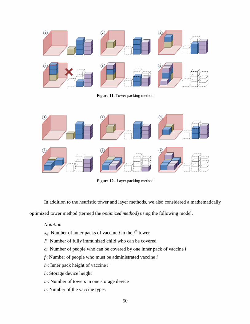
In the tower method we used a first-fit-decreasing heuristic where inner packs were stacked in

decreasing order of height in a single tower until no more can be placed in that tower, and we

then search for the largest inner pack that fits in the remaining space (Figure 11). When no inner

packs can be fitted into the current tower a new tower is started and this procedure is repeated

until all inner packs are exhausted. In the layer method, the inner packs are sequentially placed in

the same layer in decreasing order of height until there is no more space in the layer to form

several different towers. These towers are then built up layer by layer in a sequential fashion

until all inner packs are exhausted (Figure 12).

49

Figure 11. Tower packing method

Figure 12. Layer packing method

In addition to the heuristic tower and layer methods, we also considered a mathematically

optimized tower method (termed the optimized method) using the following model.

Notation xij: Number of inner packs of vaccine i in the jth tower

𝐹𝐹: Number of fully immunized child who can be covered ci: Number of people who can be covered by one inner pack of vaccine i fi: Number of people who must be administrated vaccine i hi: Inner pack height of vaccine i h: Storage device height

m: Number of towers in one storage device

n: Number of the vaccine types

50

𝑀𝑀𝑀𝑀𝑥𝑥 𝐹𝐹 (45)

subject to

𝑐𝑐𝑖𝑖 �𝑥𝑥𝑖𝑖𝑖𝑖

𝑚𝑚

𝑖𝑖=1

≥ 𝐹𝐹 for 𝑖𝑖 = 1 to 𝑛𝑛 (46)

�ℎ𝑖𝑖

𝑛𝑛

𝑖𝑖=1

𝑥𝑥𝑖𝑖𝑖𝑖 ≤ ℎ for 𝑗𝑗 = 1 to 𝑘𝑘 (47)

𝑥𝑥𝑖𝑖𝑖𝑖 = {0, 1, 2, … } (48)

The objective (45) is to maximize the number of fully immunized children 𝐹𝐹 that can be

covered by the combination of inner packs of each vaccine in one storage device. Constraint (46)

insures that the number of FIC cannot exceed the number of people who can be administrated

each vaccine type. Constraint (47) insures that the sum of height of the inner packs in each tower

must be less than the height of the storage device. Constraint (48) insures that we only use

integral numbers of inner packs (no partial inner packs are allowed.) This model determines the

optimal way to combine the inner packs into towers to attain the maximum possible FIC value.

This linear integer programming model is presented mainly as a point of reference for bounding

the performance of our heuristic approach, since it is unrealistic to expect that this approach will

be used in the field.

51

3.3 RESULTS

3.3.1 Conventional packing efficiency

The number of children who can be fully vaccinated with each vaccine type for the conventional

inner packs is shown in the bottom row of Table 9 and the maximum expected FIC served by a

single storage device is 123. The resulting configuration of inner packs within the device is

illustrated in Figure 7.

Currently, the FIC-optimizing configuration of conventional inner packs occupies 16.71

liters, representing 81.93% of the available volume of the RCW25; we refer to this as the volume

efficiency of the packing. Although there is not enough empty space to add an inner pack of the

vaccine currently determining the maximum FIC value (Rotarix), we can still use this space for

other vaccines if we wish to do so. Thus, after filling the device to its FIC capacity, it is possible

to add in two inner packs of Yellow Fever or two inner packs of Tetanus or one inner pack of

each (the inner packs of these two vaccines are the same size). The occupied volume and volume

efficiency now rise to 17.22 liters and 84.4% respectively. Figure 8 illustrates the arrangement

with one extra inner pack of yellow fever (on top of the previous three) and one extra inner pack

of tetanus (stored vertically in the empty space shown in Figure 7).

It is important to note that these packing efficiencies were achieved by evaluating many

different possibilities and therefore almost certainly reflect a higher packing density than would

be achieved in practice, since storage devices are generally not packed and repacked multiple

times. Thus, it is not likely that this high a degree of space utilization is regularly achieved in

actual practice

52

3.3.2 Conventional versus modular packing efficiency

The maximum FIC that can be served by one RCW25 given the current inner pack sizes is 123 as

calculated above; the same methodology can be applied using the modular inner pack data and

the results are shown in Table 11 (detailed information about the numbers of doses and inner

packs achieved with conventional packing and each modular packaging system can be found in

Table 12). The results also show that the tower method often outperforms the layer method and

the optimized method always performs as well as or better than the layer and tower methods in

terms of vaccine storage. In the discussion below we use the term “baseline” or “base” to refer to

the 123 FIC obtained with conventional packaging.

Table 11. Maximum FIC and occupied volume for different proposed modular vaccine vial diameters

Diameter (cm)

Layer Method Tower Method Optimization Method FIC Vol. % FIC Vol. % FIC Vol. %

2.2 (10 vials)

152 (96.2%) 92.6% 155

(98.1%) 94.1% 158 (100%) 94.8%

1.6 (20 vials)

138 (87.3%) 81.3% 148

(93.7%) 86.6% 158 (100%) 90.6%

1.9 (50 vials)

148 (100%) 87.9% 148

(100%) 87.9% 148 (100%) 87.9%

Mix 1.6+2.2

148 (93.7%) 87.4% 145

(91.8%) 86.1% 158 (100%) 91.5%

Note that the numbers below the FIC in the parentheses is the percentage

Generally speaking, all modular packing systems exceed baseline packing efficiency,

both in terms of maximum FIC served and volume efficiency. For example, using modular inner

packs with vial diameter 2.2 cm, 155 FIC can be served per storage device, with a 94.1% volume

efficiency, when the tower method is applied. It is also worth noting that (a) this increase in

53

efficiency is mainly because of the new inner pack sizing and is not dependent on the specific

approach used to store the inner packs within the device, and (b) potential improvements are

likely to be even higher because any optimization of conventional packing in the field is highly

unlikely and in reality the actual FIC figure attained is likely to be much lower that our baseline

value of 123, which was obtained after significant effort. For catchment areas with higher

populations where larger volumes of vaccine are required, this has the potential for reductions in

the number of vaccine carriers required and/or reductions in the replenishment frequency, which

in turn could yield lower transportation and personnel costs. Estimating such potential savings

would be the next step in analysis of this novel modular packaging system.

54

Table 12. Total doses, inner packs, and FIC by antigen for conventional versus proposed modular packaging configurations within the Dometic RCW25

BCG Tetanus Measles Oral Polio Yellow Fever DTP-HepB-Hib PCV13 Rota

Total

Doses Inner Packs

Total Doses

Inner Packs

Total Doses

Inner Packs

Total Doses

Inner Packs

Total Doses

Inner Packs

Total Doses

Inner Packs

Total Doses

Inner Packs

Total Doses

Inner Packs FIC

Conventional Packaging Configuration 1000 1 300 3 500 1 2000 1 300 3 400 2 400 8 250 5 123

Proposed Modular Packaging Configuration

2.2 cm Vial Diameter Layer Method 400 2 400 4 300 3 800 4 300 3 480 24 470 47 310 31 152 Tower Method 400 2 400 4 300 3 800 4 300 3 500 25 470 47 320 32 155 Tower Opt. Method 400 2 400 4 300 3 800 4 300 3 500 25 480 48 320 32 158

1.6 cm Vial Diameter Layer Method 400 1 400 2 400 2 800 2 400 2 440 11 420 21 280 14 138

Tower Method 400 1 400 2 400 2 800 2 400 2 480 12 460 23 300 15 148 Tower Opt. Method 400 1 400 2 400 2 800 2 400 2 520 13 480 24 320 16 158

1.9 cm Vial Diameter Layer Method 1000 1 500 1 500 1 1000 1 500 1 500 5 450 9 300 6 148


1.6 + 2.2 cm Vial Dia. Layer Method 400 2 400 4 300 3 800 2 300 3 480 12 460 23 300 30 148


55

3.4 ANALYSIS WITH MORE STORAGE DEVICES

Even though the RCW 25 is a widely used cold box, many other devices are used in practice and

the modular packaging which is designed for the RCW 25 could be used with other storage

devices. The question of interest is, if this occurs, does this modular packaging still work better

than conventional packaging? In order to answer this, the space efficiency of the modular

packaging system is examined using the same analysis method used in the previous research by

evaluating the modular packaging configurations for the RCW 25 when they are applied to

another storage device.

3.4.1 Selection of the new device

First, we consider the storage devices found in the WHO’s pre-qualified storage device list that

have similar volumes to that of the RCW 25. These devices are shown in Table 13.

Table 13. WHO pre-qualified storage device list

PQS code Model Length(cm) Width(cm) Height(cm) Volume(liter) E004/025 CB-20-CF 53 23 20 24.4 E004/031 AICB 503 L 45.5 31 16 22.6 E004/015 ACB 503L 45.5 30.5 16 22.2 E004/024 ACB 316 L 44.2 29.3 18.3 23.7 E004/014 ACB 444 L 45 29.4 16.4 21.7 E004/013 RCB 444 L 23 45 30 17 23.0 E004/010 AICB 444 L 44.8 30 16.7 22.4 E004/036 RCB 444L-A 45 30 15 20.3

56

Seven of the storage devices have dimensions of about 45 cm in length and 30 cm in

width. Since the volume of the RCW 25 is 20.3 liters, the RCB 444L-A which has 20.3 liters

volume is chosen to analyze the space efficiency of the modular packaging system.

3.4.2 Results for the new device with the inner pack configurations for the RCW 25

When the original inner pack sizes are used, the RCB 444L-A can store vaccines that are able to

cover 126.6 FICs. Note that this packing configuration was found by evaluating numerous

configurations and represents a packing density that would be difficult to achieve in practice.

Table 14 shows the number of FICs when the modular inner packs which were created for the

RCW 25 are used to fill the RCB 444L-A. When 1.6 cm diameter vials are used, a maximum of

21 (3 × 7) tower are available in the RCB 444L-A. For 2.2 diameter vials, a maximum of 20

(4×5) tower are available. When the inner packs are stored vertically in the tower, 112.2 FICs

can be covered when using 1.6 cm diameter vial inner pack with the tower method, and 118.8

FICs for 2.2 cm diameters with the layer method. Since the inner pack dimensions are not

designed for the RCB 444L-A, after filling up the tower in the storage device, there are spare

spaces where additional inner packs can be stored. If the spare space is used to store vaccines,

the FICs for the 1.6 and 2.2 diameter vial inner packs increase to 145 with the layer method and

152 with the tower method each.

57

Table 14. FIC for the heuristic and optimizing methods

Proposed Modular

Packaging Configuration

No. of tower1)

Tower method Layer method Optimizing method

In towers2)

+ Spare space3)

In towers2)

+ Spare space3) In tower2) + Spare

space3)

1.6 cm diameter 21 112.2

(100%)4) 138.6

(87.4%) 110.0 (98%)

145.2 (91.6%) 112.2 158.6


(97.3%) 152.0 (98%)

112.2 (91.9%)

145.7 (93.9%) 122.1 155.1


(100%) 126.6

(85.2%) 99.0

(100%) 126.6

(85.2%) 99.0 148.5

1.6 cm +2.2 cm mixed 20 114.0

(96%) 151.8

(100%) 110.0

(92.6%) 138.6

(91.3%) 118.8 151.8

1) The footprint of a tower is the area that one modular inner pack takes in the storage device.

2) When vaccines are filled only in towers 3) When vaccines are filled in towers and any empty space after filling the towers 4) Percentage ratio of the FIC of the tower/layer method to the optimizing method

When the inner packs are stored only in towers, the number of FIC is less than 126.6.

However, when we consider that 126.6 is not the number of FIC that we can expect to attain in

practice, the value that we obtain with only tower packing is reasonably good. In addition,

because the spare space can be utilized to store more inner packs, the modular packing systems

exceed the baseline packing efficiency. Clearly, the optimizing method provides better results

than the two heuristic methods, but the FIC difference between the heuristic methods and the

optimizing method is relatively small so the heuristic methods can be used to fill the storage

devices almost as well as the optimizing method does.

58

3.4.3 New configuration for the RCW 25 and the new device

Now, we consider new modular configurations that consider the size of the RCW 25 and the new

device. These configurations allow more modular inner packs to be stored than the modular

configurations designed for only the RCW 25. Using the same methods as in section 3.2.2, the

proper inner pack dimensions are chosen and shown in table 15.

Table 15. New modular packaging configuration for RCW 25 and RCB 444L-A

New Modular Packaging

Configuration BCG-20 TT Mea TOPV YF DTP-

HepB PCV13 RV

1.76 (20 vials per pkg)

8.8 8.8 8.8 8.8 8.8 8.8 8.8 8.8 7.04 7.04 7.04 7.04 7.04 7.04 7.04 7.04 6.81 8.22 6.81 4.58 8.22 3.23 4.36 5.56


8.82 8.82 8.82 8.82 8.82 8.82 8.82 8.82 7.35 7.35 7.35 7.35 7.35 7.35 7.35 7.35 3.51 4.24 3.51 2.36 4.24 1.67 2.25 2.87


7.5 7.5 7.5 7.5 7.5 7.5 7.5 7.5 6 6 6 6 6 6 6 6

9.38 11.32 9.38 6.30 11.32 4.45 6.00 7.66


7.488 7.488 7.488 7.488 7.488 7.488 7.488 7.488 6.24 6.24 6.24 6.24 6.24 6.24 6.24 6.24 4.88 5.89 4.88 3.28 5.89 2.31 3.12 3.98


22.47 22.47 22.47 22.47 22.47 22.47 22.47 22.47 9.55 9.55 9.55 9.55 9.55 9.55 9.55 9.55 4.61 5.56 4.61 3.10 5.56 2.19 2.95 3.76

Table 16 shows the number of the towers for each device for different vial diameters. The

1.76 cm and 2.45 diameter vial inner packs have a similar width and length, so they can be used

interchangeably. The 1.5 cm and 2.08 diameter vial inner packs also have a similar width and

length and can be used interchangeably, but only 28 towers in the RCW 444L-A are available

when they are used interchangeably.

59

Table 16. The number of the towers for RCW 25 and RCB 444L-A

New Modular Packaging Configuration

RCW 25 RCB 444L-A


15 towers (3 × 5) 20 towers (4 × 5)

2.45 cm (10 vials per pkg)

15 towers (3 × 5) 20 towers (4 × 5)


20 towers (4 × 5) 30 towers (5 × 6)


20 towers (4 × 5) 28 towers (4 × 7)


4 towers (2 × 2) 6 towers (2 × 3)

However, note that these new configurations might not be realistic because the heights of

some vials are too short to hold vaccine. Vials less than 3 cm in height may not be tall enough to

hold vaccine. The short vials occur because the vial size change only considers total vial volume

and ignores the vial shape. For example, DTP-HepB inner packs with diameter 2.45 cm have a

height of 1.67 cm, which is definitely too short.

3.4.4 Results with new configurations

Table 17 shows the number of FICs for each device when only towers are used for packing. In

most cases, a modular packaging system can hold more vaccines, as measure by FIC, than the

conventional packaging configuration (123.6 for the RCW 25 and 126.6 for the RCB 444L-A).

Note that we do not consider filling any additional spare space so as to simplify the packing

analysis. Using the spare space permits a storage device to hold more vaccine but makes the

packing procedure more complicated because a health worker has to consider many different

ways to utilize the spare space. In addition, even without utilizing the spare space, the modular

packaging results in better filling of the storage devices than conventional packaging.

60

Table 17. FIC for RCW 25 and RCB 444L-A with new configurations

New Modular Packaging

Configuration

RCW 25 RCB 444L-A

Tower Layer Optimizing Tower Layer Optimizing

1.76 cm 138.6 (99.5%)1)

132 (94.6%) 139.3 132

(88.9%) 138

(92.9%) 148.5

2.45 cm 143.6 (98.6%)

138.6 (95.1%) 145.7 143.6

(92.6%) 145.2

(93.6%) 155.1

1.5 cm 132 (100%)

118.8 (90.0%) 132 151.8

(92.2%) 151.8

(92.2%) 164.7

2.08 cm 138.6 (100%)

135.3 (97.6%) 138.6 141.9

(93.5%) 145.2

(95.7%) 151.8

2.14 cm 115.5 (93.3%)

123.8 (100%) 123.8 148.5

(100%) 148.5

(100%) 148.5

1) Percentage ratio of the FIC of the tower/layer method to the optimizing method

Obviously, the FIC for the RCW 25 decreases and the FIC for the RCB 444L-A

increases. When the vial configurations for the RCW 25 are used and only the tower space is

used, the maximum FICs for each device are 158.0 and 122.1, respectively. However, when the

new configurations for both devices are used and only the tower space is used, the maximum

FICs for each device are 145.7 and 155.1, respectively. This implies that the new packaging

configuration results in greater vaccine storage if equal numbers of the two devices are used.


The results of this study show that modular inner packs permit more vaccines to be stored in the

storage device. This follows from the fact that we choose to standardize vial diameters and inner

pack sizes, which in turn leads to easier and more efficient packing in a vaccine carrier. Under

the current situation with widely varying inner pack sizes it is not possible to arrive at a

consistent and space-efficient packing arrangement. Additionally, the modular inner packs would

actually provide even greater packing efficiency because the height of the inner packs was

61

determined conservatively in our analysis; adjusting for this will likely increase the packing

efficiency difference by approximately an additional 5%. We also recommend the tower

approach over the layer approach since the former generally provides slightly better packing

efficiency. The mathematical model allows more vaccine to be stored in the storage device, but

the heuristic methods also provide good packing efficiency in all examples. Therefore, if the

optimizing method is not available, the heuristic ones can provide a good packaging solution.

Finally, the optimized tower approach would be unrealistic in practice and its results serve

mainly to provide an upper bound on performance. Table 11 shows that the heuristic methods do

well in relation to this bound.

Since different shapes and sizes of storage devices are used in practice, it is impossible to

design a modular packaging scheme that fits all storage devices precisely. However, if there is a

commonly used storage device in a country and it is possible for the vaccine manufacturers to

manipulate the size of the modular packaging, then selecting the right dimension that give a

precise fit for the device would be a good strategy to employ. Even if there are different storage

devices in a country, as long as a modular packaging system is utilized, more vaccines can be

packed than when conventional packaging is used. We also accrue additional benefits from using

modular packaging including simple, consistent and fast packing, ease of counting the number of

vials, and easier handling in general.

It should be noted that if the demand is not high enough to warrant filling the cold box

(e.g., at a catchment area with a low population) then packaging is obviously less of an issue.

Simply filling the carrier with additional vaccines to maximize FIC might not be appropriate if

there is potential for wastage of excess vaccines at such locations. The issue of packaging is of

greater importance when we have sufficient demand and the cold boxes we have cannot take

62

everything needed because of the inconsistent packaging sizes, or when inconsistent sizes make

it difficult for health care workers to manage limited space in a simple and efficient fashion.

In summary, there are several advantages to using the modular packaging as listed below;

the first two are probably the most important.

1. It achieves higher packing densities for a reasonable packing method such as the tower or

the layer approach, as indicated by the data in Table 3-5. Also, recall that the heights of

the modular inner packs were found by using conservative volume estimates and

therefore the actual packing density differences between conventional and modular

systems will likely be a few percentage points greater. It is also important to note that the

conventional packing densities discussed assume that packers optimize space efficiency

by packing and re-packing to achieve maximum efficiency. Thus, the packing densities

achieved in practice are probably lower, which further increases the advantage of using

the modular systems.

2. The modular packing procedure is much simpler and more consistent. Vaccines are

simply stacked vertically in the twenty or six vertical stacks (depending on the vial size);

there is no need to explore numerous complicated orientations and geometrical

configurations. Thus, high packing efficiencies can be obtained consistently with little

effort or special expertise required. This is a tremendous advantage from a practical

standpoint because the personnel packing the storage devices will not require special

training to ensure that carefully planned packing procedures are followed routinely in the

field.

3. The simplified modular packing procedure will be faster since the person packing the

storage device does not have to spend time exploring different configurations.

63

4. Counting the number of vials is easier because the inner packs have uniform quantities

(this advantage is somewhat reduced if more than one standard size is adopted).

5. It is easier to handle the inner packs because they are all the same size, rather than trying

to handle vaccines with different inner pack sizes. For example, transporting a stack of

vaccines that has an inner pack that is 12cm × 15cm on top of an inner pack that is 15cm

× 18cm which is on top of an inner pack that is 20cm × 20cm is more difficult to do

without toppling it than a stack of three inner packs that all have the same dimensions.

6. Ideally, the vaccines should be packed with about 1cm of clearance space in between

each inner pack to promote good air flow and uniform cooling (especially in

refrigerators). If the inner packs have a consistent modular size, this would facilitate

inserting spacers in between the stacks of inner packs to insure proper clearance is

maintained.

7. If the inner packs are a consistent size, then cold storage devices can be manufactured

with storage spaces that have dimensions that most efficiently accommodate the inner

packs.

These benefits comes from the power of standardization. In this chapter, we have focused

on standardization of vaccine packaging by changing packaging configurations. The modular

packaging designed for a storage device can decrease wasted space in the storage device and can

make it possible to utilize easy stacking methods. If the storage devices are also standardized

along with the modular packaging size, the space efficiency could be maximized over an entire

country.

While our analysis suggests that modular packaging systems offer benefits over

conventional vaccine packaging in the form of increased potential FICs, higher packing

64

densities, and simplifying the process of a worker packing a storage device, there are several

limitations to our study. First, we assumed a single conventional packaging type for each existing

vaccine, while it is likely that existing packaging varies for vaccines from different

manufacturers or with different dose schedules. Similarly, in designing a potential modular

packaging system, we assumed that all vaccines could fit in new, optimized vials based on the

volumes of vials currently in use. This may not be the case for all existing vaccines. Third, our

packing approach is a heuristic algorithm related to inner pack heights and if these heights are

widely different it might not provide packings that are as good as the ones in our illustration.

Finally, in order to quantify the economic benefits of improved packaging, a potential next step

would be to utilize a vaccine supply chain modeling software, such as HERMES(Assi, et al.,

2011; Lee, et al., 2011; Assi, et al., 2013), to determine the economic impact of changing

packaging sizes. The impact could vary significantly depending on the country and

circumstances (e.g., vaccine regimen), and such an analysis would require extensive simulation

experiments and could be the basis of a future study.

Our analysis suggests that modular packaging systems could offer significant advantages

over conventional vaccine packaging systems with respect to space efficiency when combined

with a reasonable packing method such as the layer or tower method, when they are stored in

standard vaccine carrying devices. This allows for more vaccines to be stored within the same

volume while also simplifying the procedures used by field workers for packing storage devices.

Ultimately, this could be a simple way to help increase vaccine coverage worldwide.

65

4.0 APPLYING LEAN CONCEPTS TO MANAGE VACCINE INVENTORY

4.1 INTRODUCTION

Vaccines administered at clinics or health centers are typically supplied from an upper level

distribution location. The replenishment of vaccines at a clinic usually happens at regularly

scheduled intervals (e.g., once a month) and requires completing vaccine ordering processes such

as determining how many vaccine doses remain and requesting the amounts necessary to cover

the forecast demand before the next replenishment. This vaccine ordering process is executed by

health workers at clinics across the country. It is complicated by the fact that there might be five

to ten different vaccine types (e.g., measles, DTP, polio, etc.) and also that vaccines come in

multi-dose vials where the number of doses in a vial is different for different vaccine types. In a

typical clinic, the health worker counts and records the remaining vaccine vials and translates

this into a number of doses. He then determines how many net doses would be required to meet

the forecast demand until the next replenishment point and translates this into the number of

vials needed for the next inventory cycle. This is done for each different vaccine and a combined

order for vials is then placed with the higher level.

At the upper level distribution location another health worker counts the number of vials

ordered by the clinic for each vaccine type and prepares them for delivery to or pickup by the

clinic. The same distribution location will typically service a number of different clinics in a

66

similar fashion. The vaccines are then transported to the clinic. Currently, an individual vial is

used as the ordering unit at the clinic, and since this is the smallest physical unit in the

distribution chain, ordering in vials (as opposed to cases or standard packs of vials) does help to

minimize clinic vaccine inventory. This is important because cold storage capacity for vaccines

can often be quite limited at clinics. However, personnel at clinics who perform logistical

activities are often poorly trained and lacking in the skills to effectively perform these activities.

The steps in the replenishment process can be tedious and even trained workers can make

mistakes in counting and recording the number of remaining vials of several different kinds of

vaccines, and managing and replenishing inventory at the individual vial level requires

significant effort. Moreover, Steele (2014) reports that immunization supply chain functions are

frequently performed in developing countries by pharmacists, clinicians and drivers, as opposed

to workers who are trained specifically on supply chain functions. She points out that vaccine

supply chain practices are poor because of poor monitoring systems, resulting in poor data for

demand forecasting and long procurement processes.

In this chapter, we conduct an ordering policy analysis with respect to the ordering unit,

and based on this analysis we recommend the use of inner packs (the next larger packaging unit),

rather than a vial, when ordering vaccines. In addition to simplifying the ordering process used

by healthcare workers at the clinics, we show that it reduces the likelihood of vaccine stockouts

and thus also improves overall vaccination levels at clinics by giving the patient more

opportunities to get vaccinated. The basic idea behind this simplified ordering process draws

upon the Kanban concept from Just-In-Time (JIT) inventory systems. JIT is a commonly used

technique in the manufacturing industry that was popularized by Toyota, and a Kanban is a

simple visual system that is used for implementing JIT. JIT/Kanbans have been shown to yield

67

considerable benefits in production settings, including simpler processes, more timely deliveries,

increased responsiveness, increased firm profitability, and inventory reductions (Monden, 2011;

Baudin, 2004; Fullerton & McWatters, 2001). In addition to manufacturing, Kanban/bin supply

systems are being adapted elsewhere and have been shown to provide better inventory control in

many healthcare settings, e.g., managing critical nursing supplies (Southwest solutions group,

2015) and other items (Graban, 2011). Rahn (2010) explains why the Kanban method has

advantages over the commonly used PAR-level system for hospital material management (where

items are replenished every period to bring inventories back to some base stock level). He

emphasizes seven main advantages including the fact that no counting is needed, and that it

promotes better inventory management practices. The primary disadvantage is that this approach

might need more physical storage space.

The remainder of this chapter is structured as follows. First, the problem is described and

the suggested ordering policies are explained. Next, we perform a storage space analysis at the

clinic level, with a focus on cold storage requirements. In this section, the methodology and

equations related to the different ordering policies are presented, and numerical examples are

illustrated using real data from two countries – Benin and Niger. Third, we perform storage

space analysis in vaccine transportation between different levels in the supply chain to

investigate the effect of the proposed ordering polices. We end with a brief discussion of our

conclusions.

68

4.2 PROBLEM DESCRIPTION

In this research, we focus solely on the ordering process at the clinic level where vaccinations

occur. Currently, the vial is the ordering unit and a base-stock policy is applied. Each period the

health worker counts the remaining vials of each vaccine, records these numbers and then orders

the number of vials needed to return to an inventory level equal to the average demand during

the replenishment cycle. Note that for some vaccines the shelf life is limited once the vaccine

vial has been opened and any vaccine remaining after this period has to be discarded. Such

wastage is referred to as open vial waste (OVW) and this has been studied by Lee et al. (2010),

Dhamodharan & Proano (2012) and Mofrad et al. (2014). The demand forecast is first inflated by

a factor to account for the percentage of OVW (where applicable) to compute the number of

vials needed and a buffer factor is added to account for demand variability. Using a base stock

level (in vials) equal to the average adjusted demand plus a 25% buffer is a standard

recommendation of the WHO (World Health Organization, 2014).

The upper level health worker receives order requests from the clinics and then picks the

corresponding vials for each clinic and prepares them for shipment. All of the vial counting for

all of the vaccines at both the clinic and the upper level is done manually and there are ample

opportunities for ordering and order fulfillment errors. Since manufactures distributed vaccine

vials in inner packs that typically range in size from 10 to 200 vials in one inner pack depending

on the vaccine type and manufacturer, we propose two ordering policies based on inner packs

and compare them with the current policy, which uses a vial as the unit.

The first proposed policy is referred to as the inner pack unit ordering policy, where a

clinic orders vaccines only in inner pack units. For a given vaccine, the clinic worker counts the

number of unopened inner packs and individual vials in any open pack to determine the number

69

of vials remaining and then calculates the required number of vials based on the forecast

demand. This policy still requires some counting of vials to obtain the number remaining, but

since there is at most one open inner pack at any time for a given vaccine, the worker only has to

count the number of remaining vials in this one inner pack. For example, if an inner pack

contains 20 vials and we have one unopened inner pack and one open one with 11 vials in it,

only the latter would be counted to determine the current inventory of 31 units. If we require 55

vials for the next cycle (typically, one month), this means we need to order 24 more vials. Since

ordering is based on rounding up to the next full inner pack, two inner packs are ordered. At the

upper level the order fulfillment process is even simpler because only full inner packs are

handled and no individual vial counting is required.

The second policy is referred to as a kanban ordering policy, where each empty inner

pack is set aside in a specified location. The worker only counts the number of empty inner

packs at the location for each vaccine and orders enough material to replenish these.

Alternatively, one might follow a process like the one common in many manufacturing

environments where each container - or inner pack in our case - is placed in its own slot

(possibly, a location that is marked with a prominently marked symbol or color). When the inner

pack is completely emptied it is discarded and the slot is empty (or the symbol is exposed), and

this represents the fact that a replacement is required for it, so that we order as many inner packs

as there are empty slots. In this context, each inner pack corresponds to a Kanban bin and the

number of bins replenished is equal to the number fully consumed. This Kanban ordering idea is

borrowed from the traditional Kanban materials management system for lean and just-in-time

production. It most closely resembles a signal Kanban (Monden, 2011). An example signal

Kanban is shown in Figure 13 where there are three measles inner packs that are stored. At the

70

time of reorder the healthcare worker simply orders the number of inner packs equal to the

number of empty storage locations. Thus, only one inner pack is ordered in case (a) and two are

ordered in case (b).

Figure 13. Signal Kanban example

The primary advantage of simplifying the ordering method is that it is easier to

implement when the personnel involved might not be well trained, and it reduces potential errors

that could occur during ordering. However, one drawback of the Kanban based idea is that it

does require more storage space at the clinic. This is because the maximum number of vials

stored under the current vial unit ordering method is equal to the order up to level, but if the

inner pack unit or Kanban ordering policy is applied, the maximum amount stored will generally

increase. In addition, a cold storage device used in transportation between points in the

distribution chain may not be able to hold all of the vaccines, because filling the storage device

with only inner packs both potentially increases the number of vials that must be transported and

also decreases packing efficiency due to having to pack the physical dimensions of the inner

pack rather than individual vials. In order to address these space issues, we evaluate the effect on

storage space at the clinic level and in transportation in the following sections.

71

4.3 CLINIC STORAGE DEVICE ANALYSIS

Introducing the simplified ordering policies of the previous section generally leads to needing

more storage space at the clinic because vaccines are now ordered in inner pack units. In order to

evaluate the effect of the two proposed policies on incremental space requirements, we perform a

clinic storage device analysis. To understand the true impact at a high level, we use real data to

calculate the total number of storage devices needed across the entire set of clinics in a country

in order to store vaccines for each policy, and we repeat these calculations for different inner

pack sizes. Since a public health decision maker would not want the number of storage devices

to increase significantly due to the resulting increase in system-wide costs, our goal is to also

determine an inner pack size that results in only a modest increase in the required number of

storage devices country-wide.

4.3.1 Methodology

The total number of storage device needed is estimated conservatively by summing the minimum

number of storage devices required at each location for each ordering policy. This can be

computed using several pieces of available information: the monthly demand, the average

number of vaccination days per week, device storage volumes, and vaccine information such as

dose(s) per patient, number of doses per vial and packed volume per vial. The first step is to

estimate the average total number of doses needed per vaccination day for vaccine 𝑖𝑖 at location 𝑗𝑗

(= 𝑠𝑠𝑖𝑖𝑖𝑖 ) as follows:

𝑠𝑠𝑖𝑖𝑖𝑖 = �𝑑𝑑𝑖𝑖𝑀𝑀𝑖𝑖� × 𝑝𝑝𝑖𝑖 (49)

72

where 𝑑𝑑𝑖𝑖 denotes the patients per month expected at location/local clinic 𝑗𝑗, 𝑀𝑀𝑖𝑖 denotes the

number of vaccination days per month at location 𝑗𝑗, and 𝑝𝑝𝑖𝑖 denotes the doses per patient of

vaccine 𝑖𝑖.

Next, we calculate the number of vials 𝑘𝑘𝑖𝑖𝑖𝑖 required per month for vaccine 𝑖𝑖 at

location 𝑗𝑗, as follows:

𝑘𝑘𝑖𝑖𝑖𝑖 = ��𝑠𝑠𝑖𝑖𝑖𝑖

1− 𝑓𝑓𝑜𝑜𝑜𝑜(𝑠𝑠𝑖𝑖𝑖𝑖, 𝑜𝑜𝑖𝑖)�×

𝑀𝑀𝑖𝑖𝑜𝑜𝑖𝑖� × (1 + 𝑏𝑏)� (50)

where 𝑜𝑜𝑖𝑖 denotes the number of doses per vial of vaccine 𝑖𝑖, 𝑓𝑓𝑜𝑜𝑜𝑜 is the open vial waste which is

a function of 𝑠𝑠𝑖𝑖𝑖𝑖 and 𝑜𝑜𝑖𝑖, and 𝑏𝑏 denotes the buffer value; the (1 + 𝑏𝑏) term is used to add a buffer

to account for variability in the patient arrival process.

Because 𝑘𝑘𝑖𝑖𝑖𝑖 is the number of vials required per month, anytime the inventory level is

below 𝑘𝑘𝑖𝑖𝑖𝑖 at the beginning of the month, ordering needs to occur. Thus, 𝑘𝑘𝑖𝑖𝑖𝑖 − 1 is the largest

number of vials that can be on hand when ordering occurs. Assume we use inner packs

containing k vials. With our first (inner pack) ordering policy, we simply count the number of

vials in any currently open inner pack (say, x) and the number of unopened inner packs (say, y)

and if 𝑘𝑘𝑦𝑦 + 𝑥𝑥 < 𝑘𝑘𝑖𝑖𝑖𝑖 we place an order for ⌈(𝑘𝑘𝑖𝑖𝑖𝑖 − 𝑘𝑘𝑦𝑦 − 𝑥𝑥)/𝑘𝑘⌉ inner packs.

With the second (Kanban) ordering policy, we have to be more careful. Recall that we

order as many inner packs as the number fully consumed, and assume that the policy is

implemented by assigning each inner pack a slot and ordering enough to fill each empty slot.

Then the minimum number of slots to set aside (say n) is given by

𝑛𝑛 − 1 ≥ 𝑘𝑘𝑖𝑖𝑖𝑖 − 1

𝑘𝑘 (51)

73

𝑛𝑛 = �𝑘𝑘𝑖𝑖𝑖𝑖 − 1

𝑘𝑘 �+ 1 (52)

It might seem that we could simply let 𝑛𝑛 = ⌈𝑘𝑘𝑖𝑖𝑖𝑖/𝑘𝑘⌉ but this is not sufficient because we

want to ensure that when there is a partially empty inner pack (as would often occur) at an

ordering time, we order sufficient inventory. For example, suppose the inner pack size is 20, 𝑘𝑘𝑖𝑖𝑖𝑖

is 50, and we have two full inner packs plus one inner pack with 6 vials in it when we review the

inventory prior to deciding on whether to place an order. If we only set n = ⌈50/20⌉ =3 slots

then we will not order any vaccines since all three slots are currently occupied (two by full inner

packs and one by the inner pack with 6 vials). However, we will only have 46 vials on hand,

which is below our desired inventory level. Thus, the + 1 term is needed to insure that the clinic

always starts with the minimum required number of vials. Otherwise, a partially filled inner pack

(in the extreme case, with as little as one vial in it) would result in us not placing an order to

replenish that inner pack, which might cause the starting level of stock to be below the desired

amount and increases the likelihood of a vaccine shortage during that cycle. Furthermore, we

use 𝑘𝑘𝑖𝑖𝑖𝑖 − 1 rather than 𝑘𝑘𝑖𝑖𝑖𝑖 because in the case that 𝑘𝑘𝑖𝑖𝑖𝑖 − 1 is an integer multiple of the inner

pack size, using 𝑘𝑘𝑖𝑖𝑖𝑖 could result in holding one more inner pack than is strictly necessary,

because in this special case even if the last inner pack only has one vial remaining that is

sufficient. For example, if the inner pack size is 20 and 𝑘𝑘𝑖𝑖𝑖𝑖 is 61, then using n = ⌈𝑘𝑘𝑖𝑖𝑖𝑖/𝑘𝑘⌉ + 1 =

⌈61/20⌉ + 1 will result in using 5 slots. However, only 4 slots are actually required because

even if the inner pack in the last slot contains only one vial we will have sufficient vial inventory

for the month.

We made the assumption that vaccine vials are stored in inner packs in the storage device

when the inner pack unit ordering policy or Kanban ordering policy is used. Therefore, even if

only one vial is left in the inner pack the volume of one entire inner pack is still occupied. The

74

Kanban ordering policy needs sufficient space to store the number of inner packs required to

provide 𝑘𝑘𝑖𝑖𝑖𝑖 vials and then one more inner pack because inner packs are only replaced once they

are fully empty. The inner pack unit ordering policy also needs enough space to hold the number

of inner packs required to provide 𝑘𝑘𝑖𝑖𝑖𝑖 vials, plus one, because at times one inner pack may have

as few as one vial remaining but still occupies an entire inner pack’s volume. For example, let

𝑘𝑘 = 10 and 𝑘𝑘𝑖𝑖𝑖𝑖 = 14, then �𝑚𝑚𝑖𝑖𝑖𝑖−1𝑘𝑘

� + 1 = �14−110

� + 1 = 3, so space to hold three inner packs is

needed. If there are 18 vials left at the time of reordering, no vaccine is ordered under the inner

pack ordering policy (because 18 > 14), but one inner pack is ordered in the Kanban ordering

policy (because one inner pack location is empty). If there are 13 vials left at the time of

reordering, both policies order one inner pack. Thus, the Kanban and inner pack ordering

policies both require sufficient space to store the same maximum number of inner packs although

the average inventory level of the inner pack ordering policy will be lower.

To estimate the required vaccine storage volume for a vaccine we start with the packed

volume per vial (which we define as 𝑔𝑔𝑖𝑖𝑜𝑜). For vaccines that require a diluent (a liquid that is used

to reconstitute freeze dried vaccines), the diluent must also be stored in the storage device before

it is used. We assume that 10% of a vaccine’s diluent is stored in the storage device at any point

in time. Thus, the net storage volume per vial of a vaccine, 𝑔𝑔𝑖𝑖, is given by

𝑔𝑔𝑖𝑖 = 𝑔𝑔𝑖𝑖𝑜𝑜 + 0.1𝑙𝑙𝑖𝑖 (53)

where 𝑙𝑙𝑖𝑖 denotes the packed diluent volume of vaccine 𝑖𝑖. Using an inner pack of 𝑘𝑘 vials, we

need a packed volume of (𝑔𝑔𝑖𝑖 × 𝑘𝑘) units of space per inner pack, and multiplying this by the

number of inner packs required, we may estimate the minimum required volume of vaccine 𝑖𝑖 at

location 𝑗𝑗 with inner packs of size k, denoted as 𝑓𝑓𝑖𝑖𝑖𝑖𝑘𝑘, via:

75

𝑓𝑓𝑖𝑖𝑖𝑖𝑘𝑘 = (𝑔𝑔𝑖𝑖 × 𝑘𝑘) × ��𝑘𝑘𝑖𝑖𝑖𝑖 − 1

𝑘𝑘 �+ 1� (54)

So, the corresponding estimate of the number of storage devices 𝑛𝑛𝑖𝑖 needed at location 𝑗𝑗

is given by

𝑛𝑛𝑖𝑖 = �∑ 𝑓𝑓𝑖𝑖𝑖𝑖𝑘𝑘𝑖𝑖∈𝐼𝐼

𝑐𝑐𝑖𝑖� (55)

where 𝑐𝑐𝑖𝑖 is the capacity of a storage device at location 𝑗𝑗 and 𝐼𝐼 is the index set of all vaccines.

Summing these over 𝑗𝑗 ∈ 𝐽𝐽, where 𝐽𝐽 is the set of clinics, finds the total number of storage devices

needed within an entire country. In particular, if 𝑘𝑘=1 for all vaccines ∑ 𝑛𝑛𝑖𝑖𝑖𝑖∈𝐽𝐽 is the total number

of storage devices needed in the country using the vial unit ordering policy. In general, let

𝑠𝑠 = (𝑖𝑖,𝑘𝑘) ∈ 𝑆𝑆, where S is the set of pairs of vaccine types and corresponding inner pack sizes.

For example, if BCG uses an inner pack of size 20, measles one of size 10 and PCV one of size

50, then 𝑆𝑆 = {(𝐵𝐵𝐶𝐶𝐺𝐺, 20), (𝑀𝑀𝑀𝑀𝑀𝑀𝑠𝑠𝑙𝑙𝑀𝑀𝑠𝑠, 10), (𝑃𝑃𝐶𝐶𝑉𝑉, 50)}, and the total number of storage devices

needed in the country, 𝑁𝑁(𝑆𝑆), may be estimated as:

𝑁𝑁(𝑆𝑆) = ��∑ 𝑓𝑓𝑖𝑖𝑖𝑖𝑘𝑘(𝑖𝑖,𝑘𝑘)∈𝑆𝑆

𝑐𝑐𝑖𝑖𝑖𝑖∈𝐽𝐽

� (56)

Note that in this particular capacity analysis we only consider clinic cold storage space

and do not consider any transportation capacity issues.


We illustrate our approach by applying it to data from two countries: Benin and Niger. Table 18

provides summary data for these two countries. (Haidari et al., 2015; Lee et al., 2012)

76

Table 18. Summary data for Benin and Niger

Benin Niger

Number of local clinics 658 695

Number of vaccines 8 8

Vaccination days per month 5 – 28 16

Mean clinic demand (Range of clinic demands)

564 (100 - 3300)

1,083 (300 - 3,400)

Vaccine information for Benin and Niger is shown in Tables 19 and 20. Note that the

same vaccine can have a different packed volume per vial in different countries because the

vaccine might be supplied by a different manufacturer. The data also shows that different

countries can require different numbers of doses of a particular vaccine.

Table 19. Vaccine information for Benin

Name Vaccine presentation

Doses/ vial

Packed vol./ vial(cc)

Doses /person

Diluent vol./ vial(cc)

Current inner pack size

Tuberculosis Lyophilized 20 21.09 1 12 50 Tetanus Toxoid Liquid 10 25.41 2 10

Measles Lyophilized 10 21.09 1 25 50

Oral Polio Liquid 20 14.06 4 100

Yellow Fever Lyophilized 10 25.41 1 25.4 10 DTC-HepB-Hib liquid Liquid 2 9.92 3 100

PCV13 Liquid 1 17.13 3 50

Rotavirus Liquid 1 13.5 2 50 *Note that the current inner pack size is inferred from the WHO vaccine database and vaccine information for Benin

77

Table 20. Vaccine Information for Niger

Name Vaccine presentation

Doses/ vial


Doses /person

Diluent vol./ vial(cc)

Current inner pack size*

Tuberculosis Lyophilized 20 24 1 14 50 Tetanus Toxoid Liquid 10 30 3 10

Measles Lyophilized 10 21.3 1 5 10

Oral Polio Liquid 20 20 4 100

Yellow Fever Lyophilized 10 25 1 6 10 DTC-HepB-Hib liquid Liquid 1 16.8 3 50

PCV13 Liquid 1 12 3 50

Rotavirus Liquid 1 45.9 3 10 *Note that the current inner pack size is inferred from the WHO vaccine database and vaccine information for Niger

The following analysis considers inner pack sizes of 10, 20, 50, and 100, which represent

round numbers that are commonly seen in practice. The first analysis is done for Benin. If we set

the inner pack sizes of all vaccines to be the same, the total number of storage devices needed

and the annual operation costs are as follows:

Table 21. Total number of storage devices by inner pack size for Benin

Vial unit ordering Inner pack unit ordering/Kanban ordering

Inner pack size (k) 1 10 20 50 100

Total number of storage devices 664 664 670 706 1117

Annual operation costs($) 521,535 521,535 526,545 555,593 898,018

As seen in Table 21, with k=10 there is no need to purchase any additional cold storage

devices. With inner packs of k=20 vials for all vaccine, only six more storage devices are

78

needed and even when the inner pack has 50 vials there is only a modest increase in the number

of additional storage devices needed.

Given that each vaccine has its own characteristics, it follows that the inner pack sizes of

all vaccines need not be the same. To find a reasonable inner pack size for each vaccine, a

marginal volume analysis was done for each vaccine, where the inner pack size of the selected

vaccine increases but all of the others are set to 1. The results are shown in Table 22; e.g., for the

measles vaccine, using k=10, 20, 50 and 100 result in marginal increases in volume of 4%, 9%,

25% and 55%, respectively, and we could pick a size depending on the percentage increase that

we are willing to tolerate. We consider two such values, corresponding to marginal increase in

volume of up to 10% and up to 20%. The orange colored cells indicate the inner pack size

breakpoint for up to a 10% volume increase, while the blue colored cells represent the breakpoint

for up to a 20% increase. If the breakpoints are the same for 10% and 20%, then only an orange

colored cell is shown. For Tuberculosis, Tetanus Toxoid, Measles and Yellow Fever, the 10%

and 20% breakpoint volume inner pack sizes are the same (=20).

Table 22. Marginal volume increase for each vaccine Benin

Vaccines 1 10 20 50 100

Tuberculosis Volume 5,325 5,506 5,710 6,572 8,040 Increase % 0% 3% 7% 23% 51%

Tetanus Toxoid Volume 5,325 5,532 5,764 6,727 8,382 Increase % 0% 4% 8% 26% 57%

Measles Volume 5,325 5,545 5,783 6,669 8,259 Increase % 0% 4% 9% 25% 55%

Oral Polio Volume 5,325 5,439 5,568 6,101 7,017 Increase % 0% 2% 5% 15% 32%

Yellow Fever Volume 5,325 5,579 5,855 6,877 8,714 Increase % 0% 5% 10% 29% 64%

DTC-HepB-Hib liquid Volume 5,325 5,405 5,498 5,845 6,323 Increase % 0% 1% 3% 10% 19%

PCV13 Volume 5,325 5,434 5,570 6,007 6,705 Increase % 0% 2% 5% 13% 26%

Rotavirus Volume 5,325 5,443 5,595 6,135 6,955 Increase % 0% 2% 5% 15% 31%

79

Using the inner pack sizes corresponding to the 10% and 20% marginal increases in

volume for each vaccine, the total number of storage devices needed is shown in Table 23, along

with the results for the current inner pack size combination.

Table 23. The total number of storage devices by inner pack size Benin

Vial unit ordering Inner pack unit ordering/Kanban ordering

Inner pack size 1 10 20 Up to 10%

Up to 20% Current 50 100

Total number of storage devices 664 664 670 670 678 699 706 1,117

Annual operation costs($) 521,535 521,535 526,545 526,545 533,427 550,557 555,593 898,018

As seen in Table 23, with inner packs of k=50 for DTC-HepB-Hib and k=20 for all other

vaccines (up to a 10% marginal volume increase) we still require the same number of additional

storage devices (6) as the case where all inner packs are of size 20. On the other hand, using

inner packs of k=100 for DTC-HepB-Hib, k=50 for Polio, PCV13 and Rotavirus, and k=20 for

all other vaccines (up to a 20% marginal increase in volume) we require 14 additional storage

devices. Finally, if we switched to an inner pack ordering or Kanban ordering policy while

staying with the inner packs that are currently in use (as shown in Table 19), we would still need

only 35 additional devices country-wide.

Conducting a similar analysis in Niger, we picked inner pack sizes for each vaccine with

up to a 5% and up to a 10% marginal volume increase. Note that we did not consider a value of

20% because even with inner pack sizes of 100 there was only a 7% increase and vaccines do not

typically come in inner packs larger than 100 vials (Table 24).

80

Table 24. Marginal volume increase for each vaccine Niger

Vaccines 1 10 20 50 100

Tuberculosis Volume 19,788 19,813 19,841 20,275 21,093 Increase% 0% 0% 0% 2% 7%

Tetanus Toxoid Volume 19,788 19,788 19,788 20,194 20,863 Increase% 0% 0% 0% 2% 5.4%

Measles Volume 19,788 19,860 19,959 20,168 20,870 Increase% 0% 0% 1% 2% 5.5%

Oral Polio Volume 19,788 19,788 19,788 20,044 20,655 Increase% 0% 0% 0% 1% 4%

Yellow Fever Volume 19,788 19,873 19,988 20,235 21,059

Increase% 00% 0% 1% 12% 6% DTC-HepB-Hib

liquid Volume 19,788 19,788 19,788 20,017 20,180

Increase% 0% 0% 0% 1% 2%

Rotavirus Volume 19,788 19,788 19,788 20,412 20,858 Increase% 0% 0% 0% 3% 5.4%

PCV13 Volume 19,788 19,813 19,841 19,951 20,068 Increase% 0% 0% 0% 1% 1%

If up to a 5% and up to a 10% volume increase inner pack size for each vaccine are

applied, the total number of storage devices needed is shown in Table 25. Table 25 also shows

results for the current combination of inner pack sizes.

Table 25. Total number of storage devices by inner pack size for Niger

Vial unit ordering Inner pack unit ordering/kanban ordering

Inner pack size (k) 1 10 20 Current 50 Up to 5% 100/ Up to 10%

Total number of storage devices 1,057 1,068 1,068 1,122 1,177 1,188 1,499

Annual operation costs($) 679,975 686,468 686,468 716,030 747,712 755,159 850,136

The Niger results indicate that using inner packs of up to 20 for all vaccines requires only

eleven more storage devices over the entire country than with the current vial unit ordering

policy; this is a very small increase. Note that this is less than the number of storage devices

81

needed if used the new ordering policies with the current set of inner pack sizes. Choosing inner

packs of size 50 for all vaccines results in needing 120 more storage devices which represents

only about a 10% increase in the total number of devices. If we increase the inner pack sizes up

to 100 then there is a significant increase in the number of storage devices needed. We could also

use a combination of inner packs of size 20 for all vaccines except PCV13 and DTC-HepB-Hib

liquid where a size of 50 would be used (a larger inner pack is used for PCV13 and DTC-HepB-

Hib liquid because both are relatively small volume and have high demand) This results in a

need for 1,069 storage devices across the country, which is an increase of only twelve over the

single vial ordering policy. Thus, ordering logistics in Niger can be greatly simplified from both

the ordering and fulfillment viewpoints with very little impact on the number of storage devices

needed countrywide at the clinic level.

4.4 TRANSPORTATION STORAGE SPACE ANALYSIS

So far, we have only considered clinic cold storage space and not transportation capacity.

Typically, vaccines are transported to clinics in vaccine carriers, using small 4×4 vehicles,

motorcycles, bicycles or even on foot. These vaccine carriers have limited storage space and

given that inner packs take up more space in a carrier than individual vials, ordering policies that

use an inner pack unit may require more storage devices in transportation, and specific devices

might not be suitable in the first place. According to the WHO’s specifications, the capacity of

vaccine carriers which are used for vaccine vial transportation is between 0.5 and 5 liters (World

Health Organization, 2010).

82

The BK-VC 1.7-CF which is used from the District distribution centers to clinics in

Benin has a capacity of 1.7 liters. In Niger on the other hand, a 5 liter vaccine carrier is used

(Assi et al., 2013). In addition, although the average volume of vaccines transported to a clinic

might be similar, there is a higher degree of variation in the total volume required with the inner

pack policies and the packing efficiency is worse since their replenishment unit is an inner pack.

Therefore, we need to consider how using inner packs affects storage space requirements when

transporting vials to clinics.

4.4.1 Simulation model

In order to examine the effect of using inner packs on transport capacity requirements, a model is

developed using Microsoft Excel VBA to simulate a clinic’s ordering policy. We assume that the

daily demand follows a Poisson distribution, and values of these demands at each clinic j for

each vaccine i are randomly generated using a mean value of sij (as given by (49)). Monthly

orders are placed according to each of the ordering policies that we study. The simulation model

has the following parameters: inner pack size, doses per vial, whether or not the vaccine

experiences open vial waste, buffer percentage, annual number of patients served at the location,

vaccination days per month, doses per patient, and ordering policy.

The model assumes that 1) the lead time is zero, 2) back orders are not allowed, 3) the

vaccine shelf lives are long enough that expiration is not a problem, and 4) vaccines are ordered

each month. We run the simulation using the inner pack sizes found from the previous section

that analyzed storage device requirements at the clinic level. The output of the model is the

number of vials or inner packs ordered each month for each vaccine type under each ordering

83

policy; this determines the total amount of vaccine that must be transported to the clinic from the

next higher level, and hence, the required transportation storage capacity.

4.4.2 Methodology

The simulation model is run for 2000 months and for each month, and for each vaccine, it yields

either the number of inner packs (for the two simplified policies that use an inner pack unit), or

the number of vials ordered (for the current ordering policy). From this data, the volumes of the

shipments are then calculated. Since the transportation storage devices should be able to

transport the required vaccine amount of vaccine every month with a high probability, we

specify the required total volume to be such that at least 95% of all orders (as estimated from the

simulation output) can be successfully transported. This is estimated from the output of the

simulation. Using this vaccine replenishment data and the capacity of each transportation storage

device we then estimate the number of transportation storage devices required.

For the current ordering policy with vial ordering/storage, we decrease the available

space in the device to account for its packing efficiency. For example, if the capacity of a storage

device is 3 liters and the packing efficiency is 80%, the storage device can hold 2.4 liters of

vaccine vials; thus, if our requirement was for 6 liters of vaccines, we would need 3 devices.

With the two simplified ordering polices, we use a trial-and-error method for packing the

required vaccine inner packs into the physical dimensions of the transport storage device, given

their dimensions and the dimensions of the storage space in the device. While a more

sophisticated approach such as a 3D bin packing algorithm could be used, we chose to use the

simpler methods that might be used in practice by a healthcare worker in the field.

84

4.4.3 Numerical example and Result

The results from the simulation and the analysis are shown below for Benin. The transportation

storage device commonly used at clinics in Benin (BK-VC 1.7-CF) has a vaccine storage volume

of length 10 cm, width 10 cm and height 17 cm after it is packed with conditioned ice. The

average annual patient demand, which is 550, is used to determine daily demand for doses of

each vaccine. Since some of the current inner packs (Tuberculosis, Measles, DTC-HepB-Hib and

PCV13) are too large to be held in the BK-VC 1.7-CF, assessing the simplified ordering policies

with these inner packs is impossible, and the only option is to order in vial units. However, as we

saw in the storage device space analysis, 10- or 20-vial inner packs could be considered with

very little increase in clinic storage requirements. Table 26 shows the actual inner pack

dimensions for the 10-vial inner packs. Note that the new dimensions are calculated based on the

current vial diameter and height.

Table 26. 10 vial inner pack dimensions

Vaccines Tuberculosis Tetanus Measles Oral Polio

Yellow Fever

DTC-HepB-

Hib PCV13 Rota

Length(cm) 9.25 10.6 9.25 7.5 10.6 9 8.95 7.3 Width(cm) 3.8 4.7 3.8 2.5 4.7 2.98 3.68 3.4 Height(cm) 6 5.1 6 7.5 5.1 3.7 4.1 6.9

Using the current vial unit ordering policy, we need 6.39 liters to cover all orders with a

probability of 0.95, and 6.55 liters with 0.99 probability. Using the Kanban ordering policy or

inner pack unit ordering policy with 10-vial inner packs for all vaccines, 6.49 liters are needed to

cover all orders with the 0.95 probability, and 6.67 liters with 0.99 probability. Table 27 shows

the corresponding number of inner packs of each vaccine for the simplified ordering policies.

85

Table 27. Number of inner packs for the simplified ordering polices

Vaccines Tuberculosis Tetanus Measles Oral Polio

Yellow Fever

DTC-HepB-

Hib PCV13 Rota

Kanban ordering 2 1 2 1 2 8 14 12

Inner pack unit ordering 2 1 2 1 2 7 16 11

Table 28 shows the number of storage devices required to hold 6.39 liters of vaccine vials

for different packing efficiencies. For example, if an effective 80% of device storage space is

available, five storage devices are needed. In fact, if the packing efficiency is between 80% and

90%, five storage devices will suffice.

Table 28. Number of storage devices required to hold 6.39 liters of vaccine vials

Packing efficiency 70% 80% 90% 100%

The number of the storage devices 6 5 5 4

When 10-vial inner pack vaccines are used, we estimated that six storage devices are

required for both the Kanban ordering policy and the inner pack unit ordering policy to cover

95% of vaccine delivery. With 20-vial inner packs, seven storage devices are required for both

policies.

Clearly, if the inner pack size cannot be changed, the simplified ordering policies are not

practical. However, if 10 or 20 vial inner pack can be used, one or two more additional

transportation storage devices (vaccine carriers) would be required at each clinic.

86


Ordering vaccines in inner pack quantities has many advantages over single vial ordering

including convenience in managing inventories, fewer errors in counting and ordering, and

reduced order fulfillment effort. If vaccines are stored within an inner pack, a health worker can

easily distinguish vaccines from each other and more readily find the particular vaccine that the

worker is looking for because there is vaccine information on the outside face of the inner pack.

In addition, at the upper level distribution center, the complicated vial counting process to supply

clinics will be replaced by a much simpler process of picking one, or counting just a few inner

packs. Counting errors at the upper levels will decrease and order preparation and distribution

time will be saved. EPI vaccines are not particularly expensive, so there is no real disadvantage

to holding more vaccines at the clinic level, as long as there is sufficient storage space.

The results from Benin and Niger indicate that while there is no common inner pack size

that is best for all vaccines, if we use inner packs of size 10 or 20 for all vaccines only a few

more storage devices are needed. Thus, even though these simplified ordering policies increase

the storage volume needed, if we choose the proper inner pack size these negative consequences

can be minimized such that the additional number of storage devices needed is very small (on the

order of 1%). In terms of transportation storage space, the proposed ordering policies are not

practical without changing the inner pack size. However, if 10- or 20-vial inner packs are used

across all vaccines, one or two more storage devices in transportation will be required to service

orders with a high probability. Note that in general, a vaccine carrier is inexpensive (e.g., the

2009 price of a BK-VC 1.7-CF is US$ 12.00), so purchasing one or two devices would be very

affordable for a clinic. But if transportation resources are constrained it might become necessary

for an additional trip to a clinic in order to carry additional vaccine carriers. In this case the

87

transportation cost will increase and it might be difficult to implement due to time and resource

limitations.

In conclusion, we recommend adapting simplified ordering polices based on well-known

lean concepts (that are widely used in manufacturing) to a major public health sector. There are

several key managerial insights relating to this recommendation. First, only replenishing using

inner pack quantities reduces logistical effort and potential ordering errors at multiple levels of

the supply chain. This is particularly valuable in the context of lower and middle income

countries as many of the workers involved in the vaccine supply chains in these countries are not

well trained in logistics systems operations. Second, while the average inventory levels do

increase slightly with the simplified policies, the increase is minor and only causes minor

increases (less than a few percent) in the number of cold storage devices needed at facilities if

the inner pack sizes are carefully chosen. Third, transport logistics are also not impacted

significantly. Thus, we can achieve significant benefits from simplified ordering policies with

modest increases in operational costs by selecting proper vaccine inner pack sizes.

88

5.0 REDESIGN OF VACCINE DISTRIBUTION NETWORKS IN LOW AND

MIDDLE-INCOME COUNTRIES

5.1 INTRODUCTION

In many low and middle income countries supported by the Expanded Program on

Immunization, vaccines are distributed through a legacy medical supply chain. The legacy

medical supply chain consists of traditional medical facilities including a central distribution

center for the country, regional hospitals, district hospitals, and clinics. Their locations and

connections within the supply chain network (SCN) have typically been determined based on

political boundaries or the existing administrative hierarchy. Since the distribution network is not

optimized, the legacy medical supply chain is not necessarily a cost-efficient one.

In this chapter, we separate the cold chain for vaccine distribution from the legacy

medical supply chain and address it independently. The primary characteristic of this chain is

that it requires cold storage and transportation of a narrowly defined set of vaccines at controlled

temperatures of between 2 and 8°C. When the vaccine supply chain is separated from the

medical supply chain, redesigning it can be approached via mathematical models. In this chapter,

a mixed integer programming (MIP) model for designing the vaccine supply chain network is

introduced. As our analysis with real data shows, the solution of this problem can be quite

difficult, and an evolutionary strategy (ES) is therefore proposed to solve the network design

problem.

89

The remainder of this chapter is structured as follows. Section 2 describes the problem.

Section 3 presents the mixed integer mathematical model and Section 4 proposes the

evolutionary strategy to solve the problem. In Section 5, sensitivity analysis is performed.

Section 6 introduces a looping factor that is applied to the transport vehicle routing and

illustrates how to apply it. We talk about how to improve the ES in section 7. In section 8, we

describe how to use the results from the ES to enhance the MIP performance. Each section

presents its own numerical examples based on real data to illustrate the problem and solution

characteristics.

5.2 PROBLEM DESCRIPTION

EPI vaccines from foreign manufacturers typically enter a country via air or sea and are initially

stored in a central distribution center. Then via intermediate distribution centers, they are

transported to local clinics, where actual vaccinations take place. The legacy medical supply

chains in most countries have a 3, 4 or 5 tier arborescent structure. For instance, in a typical 4-

tier vaccine supply chain, vaccines move from the central distribution center to regional

distribution centers, and from a regional distribution center to district distribution centers, and

finally, from a district distribution center to clinics. However, since the distance from the main

source node, (the central distribution center), to a final sink node (a local clinic) varies widely

and the supply chain network design was not optimized, this hierarchical and arborescent

structure does not guarantee an optimal distribution scheme.

Our goal is to send vaccines from one fixed source node to a set of fixed sink nodes

efficiently. If intermediate distribution centers (hub distribution centers) through which vaccines

90

are transported from a source node to sink nodes are selected properly, the distribution network

will be more efficient. While the current network has a fixed number of tiers, this does not have

to be the case in general and we do not assume any such restriction. That is, vaccines can be

supplied to local clinics from the central distribution center through any number of hub

distribution centers, or even directly. A hub distribution center is a facility that stores vaccines

and supplies vaccines to local clinics as well as other hubs. Only the local clinic is assumed not

to have any distribution role. Hub distribution centers are selected from the current regional and

district distribution centers, which serve as a set of candidates.

This research considers several different storages devices at each facility and different

transportation modes/vehicles for transporting vaccines between facilities. Each facility is

allowed to choose its own storage devices for vaccines as well as its own transportation vehicles.

These storage devices have different capacities and a facility can have different storage devices

to hold its required volume of vaccines. Note that the storage capacity can be changed only in

discrete increments corresponding to additional devices. As with storage devices, there are

several types of capacitated transportation vehicles from which a facility can choose one. In

addition, we consider a replenishment/trip frequency along with vehicle capacity. For example, if

the total required volume at a facility in a year is 120 units and the replenishment frequency is

once a month, the required storage volume at the facility is 10 units, but if the replenishment

frequency is once every three months, 30 units of storage capacity is needed. The trip frequency

also works in the same way, e.g., if each replenishment must move 10 units and the capacity of

the vehicle is 5 units, then two trips will be required per replenishment. With respect to cost, we

consider transportation cost, storage cost, and facility operation cost. Transportation cost is

calculated using a travel distance between two nodes and increases discretely according to the

91

number of vehicle trips needed to deliver the required volume. Storage cost is also related to the

volume of required vaccines and increases discretely according to the number of storage devices

required to store the vaccines. Even though there are several vaccines handled, only the total

volume of vaccines affects the capacity of transportation and storage so that we only consider the

total volume of vaccines along arcs and at nodes. Facility operation costs are incurred when a

facility is open.

In this research, we decide the locations of hub distribution centers, the flows from the

central distribution center to local clinics through hub distribution centers, the storage devices

and their numbers at each facility, the transportation vehicles used and the number of trips

required for each vaccine flow between facilities, taking into account the assumed trip frequency

for each connection between supply chain levels.

We make the following assumptions to reflect a real vaccine supply chain:

(1) Only local clinics have demand and demands at each clinic are fixed based on the

population served by the clinic.

(2) The location of the central distribution center does not change.

(3) A hub distribution center can only be located at the current regional and district

distribution center locations.

(4) Every local clinic is supplied via a hub distribution center (or directly from the central

distribution center).

(5) Each operational facility has exactly one inbound flow except the central distribution

center, which has none.

(6) Enough vaccine should be supplied to clinics to satisfy all demand.

92

(7) If a hub is supplying another hub and is supplied by the central distribution center, it is

replenished quarterly.

(8) If a hub is supplied by another hub, it is replenished monthly.

(9) The replenishment frequency of local clinics is once a month.

(10) The storage device type at a local clinic is given.

(11) There is a required 25% buffer at each location so that the total required storage volume is

inflated by a factor of 1.25.

(12) If more than one trip to a lower level facility is required, it does not change the

replenishment frequency to the lower level facility, i.e., we assume that the multiple trips

are done on the same day.

The supply chain network design problem is well-known to the operations research

community and there are many papers as well as reviews on this topic. The p-median problem,

the uncapacitated facility location problem (UFLP), and the capacitated facility location problem

(CFLP) are introduced as the basic network location problems in many papers [e.g., (Klose &

Drexl, 2005), (Melo, Nickel, & Saldanha-Da-Gama, 2009) and (Mirchandani, 1990)]. These

location problems have been mostly studied for single level systems (Şahin & Süral, 2007).

Various extensions to these basic models have been derived, such as the capacitated facility

location problem with single sourcing (CFLPSS), the two-stage capacitated facility location

problem (TSCFLP), and the multi-commodity or multi-activity uncapacitated facility location

problem (MUFLP) (KloseA. & DrexlA., 2005). Mirchandani et al. discuss a stochastic variant of

the p-median problem (Mirchandani, Oudjit, & Wong, 1985). The uncapacitated facility

location/network design problem (UFLNDP) is introduced by Daskin et al. (Daskin, Hurter, &

VanBuer, 1993) and the capacitated facility location/network design problem (CFLNDP) is

93

introduced by Melkote et al. (Melkote & Daskin, 2001). With UFLNDP and CFLNDP, where the

facility location and network design problems are combined, similar to the problem in this

chapter, it is often more economical to change the configuration of the underlying network rather

than adding and locating new facilities (Melkote & Daskin, 2001). If a network has hierarchical

features, there are two basic distinct MIP models: flow-based and assignment-based formulations

(Şahin & Süral, 2007). Narula and Ogbu examine flow-based formulations for multi-flow

systems (Narula & Ogbu, 1979) and Şahin et al. construct a two-level multi-flow assignment-

based model (Şahin, Süral, & Meral, 2007).

More recently, hub location models have received considerable attention (Klose & Drexl,

2005). Algorithms for solving the uncapacitated hub location problem (UHLP) have been

developed by several researchers [e.g., (Klincewicz, 1996), (Ernst & Krishnamoorthy, 1998), and

(Hamacher, 2000)]. The capacitated case has been studied by several researchers, e.g., (Aykin,

1994) and (Ebery, Krishnamoorthy, Ernst, & Boland, 2000). Unlike the general models or papers

mentioned above, recent work has considered more complexities to cope with a more realistic

variety of situations. For example, Rahmaniani and Ghaderi have worked on a combined facility

location and network design problem with multiple types of capacitated links and suggested a

fix-and-optimize heuristic based on the firefly algorithm (Rahmaniani & Ghaderi, 2013).

Kalaitzidou et al. optimize multiechelon supply chain networks with generalized production and

warehousing nodes using a mathematical programming model (Kalaitzidou, Longinidis, Tsiakis,

& Georgiadis, 2014). In this model, the optimization procedure decides which mid echelon

locations produce items and which ones only distribute items.

Regarding applying genetic algorithms to supply chain problems, the first was an

application to a transportation problem used a nonstandard genetic algorithm for solving linear

94

and nonlinear transportation problems (Michalewicz, Vignaux, & Hobbs, 1991). The authors

used a matrix-based representation to represent a transportation tree. Since then, there have been

several studies on transportation problems (Bielli, Caramia, & Carotenuto, 2002; Gen,

Altiparmak, & Lin, 2006; Altiparmak, F; Gen, M; Lin, L; Karaoglan, I, 2009). For example,

Altiparmak et al. presented a solution procedure based on a steady-state genetic algorithm with a

new encoding structure for the design of a single-source, multi-product, multi-stage SCN

(Altiparmak, F; Gen, M; Lin, L; Karaoglan, I, 2009). They extended the priority-based encoding

of the transportation tree to a multi-product case. Firoozi et al. solve a three level hierarchical

supply chain, which is modeled with non-linear MIP, using a genetic algorithm (Firoozi, Ismail,

Ariafar, Tang, & Ariffin, 2013). Izadi and Kimiagrari solve the location-allocation problem with

an unknown demand function using a genetic algorithm and a Monte Carlo simulation approach

(Izadi & Kimiagari, 2014).

5.3 MIP FORMULATION

To formulate the problem we define the following notation:

Index sets

𝐶𝐶: Central distribution center ={0}

𝐻𝐻: Hub distribution centers ={1,2,…,|H|}

𝐼𝐼: Local clinics = {|H|+1,…,N}

𝐸𝐸: Edges:(𝑖𝑖, 𝑗𝑗)|𝑖𝑖 ∈ 𝐶𝐶 ∪ 𝐻𝐻, 𝑗𝑗 ∈ 𝐻𝐻 ∪ 𝐼𝐼; 𝑖𝑖 ≠ 𝑗𝑗

𝑉𝑉: Vertices: 𝐶𝐶 ∪ 𝐻𝐻 ∪ 𝐼𝐼

95

𝐿𝐿: Levels: {central (=0), hub (=1), local clinic (=2)}

𝑇𝑇: Transportation vehicles: {cold truck (=0), 4×4 truck (=1), motorbike (=2)}

𝑅𝑅: Storage devices: {cold room (=0), regional device (=1), district device (=2), local clinic

device (=3)}

𝐹𝐹: Replenishment frequency: {Quarterly (=0), Monthly (=1)}

Parameters

𝐶𝐶𝑖𝑖𝑖𝑖𝑡𝑡𝑇𝑇 : Transportation cost per km of vehicle type 𝑡𝑡 from location 𝑖𝑖 to location 𝑗𝑗 ; (𝑖𝑖, 𝑗𝑗) ∈ 𝐸𝐸; 𝑡𝑡 ∈ 𝑇𝑇

𝐶𝐶𝑟𝑟𝑆𝑆: Annual storage cost per storage device 𝑓𝑓; 𝑓𝑓 ∈ 𝑅𝑅

𝐶𝐶𝑖𝑖𝐹𝐹: Annual facility cost when the facility is level 𝑙𝑙; 𝑙𝑙 ∈ 𝐿𝐿

𝑃𝑃𝑡𝑡𝑇𝑇: Transportation capacity per trip of vehicle 𝑡𝑡; 𝑡𝑡 ∈ 𝑇𝑇

𝑃𝑃𝑟𝑟𝑆𝑆: Storage capacity of device 𝑓𝑓; 𝑓𝑓 ∈ 𝑅𝑅

𝐺𝐺𝑓𝑓: Annual number of replenishments 𝑓𝑓 ∈ 𝐹𝐹 (=4 if k=0; =12 if k=1)

𝑆𝑆: Buffer stock factor for vaccines stored at a location

𝐷𝐷𝑖𝑖𝑖𝑖: Distance (km) between location 𝑖𝑖 and location 𝑗𝑗 ; (𝑖𝑖, 𝑗𝑗) ∈ 𝐸𝐸

𝐵𝐵𝑖𝑖: Annual demand (𝐵𝐵𝑖𝑖<0, 𝑗𝑗 ∈ 𝐼𝐼) or supply (𝐵𝐵𝑖𝑖>0, 𝑗𝑗 ∈ 𝐶𝐶) volume at location 𝑗𝑗; 𝐵𝐵𝑖𝑖 = 0 for 𝑗𝑗 ∈

𝐻𝐻

Variables

𝑋𝑋𝑖𝑖𝑖𝑖: Annual flow (volume) of vaccines from location 𝑖𝑖 to location 𝑗𝑗 ; (𝑖𝑖, 𝑗𝑗) ∈ 𝐸𝐸

𝑊𝑊𝑖𝑖 ∈ {0,1}: 1 if a location 𝑗𝑗 is open, 0 otherwise; 𝑗𝑗 ∈ 𝑉𝑉

𝑌𝑌𝑖𝑖𝑟𝑟𝑓𝑓: Number of storage devices of type 𝑓𝑓 at location 𝑗𝑗 with replenishment frequency 𝑓𝑓;

𝑗𝑗 ∈ 𝑉𝑉, 𝑓𝑓 ∈ 𝑅𝑅, 𝑓𝑓 ∈ 𝐹𝐹

96

𝑍𝑍𝑖𝑖𝑖𝑖𝑡𝑡𝑓𝑓: Number of vehicle trips per replenishment from location 𝑖𝑖 to location 𝑗𝑗 using vehicle type

𝑡𝑡 with replenishment frequency 𝑓𝑓; (𝑖𝑖, 𝑗𝑗) ∈ 𝐸𝐸, 𝑡𝑡 ∈ 𝑇𝑇,𝑓𝑓 ∈ 𝐹𝐹

𝑉𝑉𝑖𝑖 ∈ {0,1}: 1 if a location 𝑗𝑗 has monthly replenishment frequency, 0 otherwise; 𝑗𝑗 ∈ 𝐻𝐻 ∪ 𝐼𝐼

𝑈𝑈𝑖𝑖𝑖𝑖 ∈ {0,1}: 1 if vaccines flow from location 𝑖𝑖 to location 𝑗𝑗, 0 otherwise; (𝑖𝑖, 𝑗𝑗) ∈ 𝐸𝐸

Our formulation is:

𝑀𝑀𝑖𝑖𝑛𝑛 � �� 2𝐶𝐶𝑖𝑖𝑖𝑖𝑡𝑡𝑇𝑇 𝐺𝐺𝑓𝑓𝐷𝐷𝑖𝑖𝑖𝑖𝑍𝑍𝑖𝑖𝑖𝑖𝑡𝑡𝑓𝑓 +��𝐶𝐶𝑟𝑟𝑆𝑆𝑌𝑌𝑖𝑖𝑟𝑟𝑓𝑓 +𝑟𝑟∈𝑅𝑅𝑓𝑓∈𝐹𝐹𝑖𝑖∈𝑉𝑉

𝑓𝑓∈𝐹𝐹𝑡𝑡∈𝑇𝑇(𝑖𝑖,𝑖𝑖)∈𝐸𝐸

𝐶𝐶0𝑊𝑊0 + �𝐶𝐶1𝐹𝐹𝑊𝑊𝑖𝑖𝑖𝑖∈𝐻𝐻

+ �𝐶𝐶2𝐹𝐹𝑊𝑊𝑖𝑖𝑖𝑖∈𝐼𝐼

(57)

𝑠𝑠𝑠𝑠𝑏𝑏𝑗𝑗𝑀𝑀𝑐𝑐𝑡𝑡 𝑡𝑡𝑓𝑓

� 𝑋𝑋𝑖𝑖𝑖𝑖𝑖𝑖∈𝑉𝑉:(𝑖𝑖,𝑖𝑖)∈𝐸𝐸

− � 𝑋𝑋𝑖𝑖𝑖𝑖𝑖𝑖∈𝑉𝑉:(𝑖𝑖,𝑖𝑖)∈𝐸𝐸

= 𝐵𝐵𝑖𝑖 𝑓𝑓𝑓𝑓𝑓𝑓 ∀𝑖𝑖 ∈ 𝑉𝑉 (58)

��𝑃𝑃𝑡𝑡𝑇𝑇𝐺𝐺𝑓𝑓𝑍𝑍𝑖𝑖𝑖𝑖𝑡𝑡𝑓𝑓 ≥ 𝑋𝑋𝑖𝑖𝑖𝑖𝑓𝑓∈𝐹𝐹𝑡𝑡∈𝑇𝑇

𝑓𝑓𝑓𝑓𝑓𝑓 ∀ (𝑖𝑖, 𝑗𝑗) ∈ 𝐸𝐸 (59)

��𝑃𝑃𝑟𝑟𝑆𝑆𝐺𝐺𝑓𝑓𝑌𝑌𝑖𝑖𝑟𝑟𝑓𝑓 ≥ (1 + 𝑆𝑆) � 𝑋𝑋𝑖𝑖𝑖𝑖𝑖𝑖∈𝐶𝐶∪𝐻𝐻:(𝑖𝑖,𝑖𝑖)∈𝐸𝐸𝑓𝑓∈𝐹𝐹𝑟𝑟∈𝑅𝑅

𝑓𝑓𝑓𝑓𝑓𝑓 ∀𝑗𝑗 ∈ 𝑉𝑉 (60)

𝑀𝑀𝑊𝑊𝑖𝑖 ≥ � 𝑋𝑋𝑖𝑖𝑖𝑖𝑖𝑖∈𝐶𝐶∪𝐻𝐻:(𝑖𝑖,𝑖𝑖)∈𝐸𝐸

+ � 𝑋𝑋𝑖𝑖𝑖𝑖𝑖𝑖∈𝐻𝐻∪𝐼𝐼:(𝑖𝑖,𝑖𝑖)∈𝐸𝐸

𝑓𝑓𝑓𝑓𝑓𝑓 ∀𝑗𝑗 ∈ 𝐻𝐻 (61)

𝑋𝑋𝑖𝑖𝑖𝑖 ≤ 𝑀𝑀𝑈𝑈𝑖𝑖𝑖𝑖 𝑓𝑓𝑓𝑓𝑓𝑓 ∀ (𝑖𝑖, 𝑗𝑗) ∈ 𝐸𝐸 (62)

� 𝑈𝑈𝑖𝑖𝑖𝑖𝑖𝑖∈𝐶𝐶∪𝐻𝐻:(𝑖𝑖,𝑖𝑖)∈𝐸𝐸

≤ 1 𝑓𝑓𝑓𝑓𝑓𝑓 ∀𝑗𝑗 ∈ 𝐻𝐻 ∪ 𝐼𝐼 (63)

��𝑌𝑌𝑖𝑖𝑟𝑟𝑓𝑓 ≤ 𝑀𝑀𝑊𝑊𝑖𝑖𝑓𝑓∈𝐹𝐹𝑟𝑟∈𝑅𝑅


�𝑌𝑌𝑖𝑖𝑟𝑟1 ≤ 𝑀𝑀𝑉𝑉𝑖𝑖𝑟𝑟∈𝑅𝑅


�𝑌𝑌𝑖𝑖𝑟𝑟0 ≤ 𝑀𝑀(1 − 𝑉𝑉𝑖𝑖)𝑟𝑟∈𝑅𝑅


𝑋𝑋𝑖𝑖𝑖𝑖 ≤ 𝑀𝑀𝑉𝑉𝑖𝑖 𝑓𝑓𝑓𝑓𝑓𝑓 ∀𝑖𝑖, 𝑗𝑗 ∈ 𝐻𝐻 (67)

𝑉𝑉𝑖𝑖 ≤ 2 − 𝑈𝑈0𝑖𝑖 −∑ 𝑈𝑈𝑖𝑖𝑖𝑖𝑖𝑖∈𝐻𝐻

|𝐻𝐻| 𝑓𝑓𝑓𝑓𝑓𝑓 ∀𝑖𝑖 ∈ 𝐻𝐻 (68)

𝑊𝑊𝑖𝑖 = 1 𝑓𝑓𝑓𝑓𝑓𝑓 ∀𝑖𝑖 ∈ 𝐶𝐶 ∪ 𝐼𝐼 (69)

𝑉𝑉𝑖𝑖 = 1 𝑓𝑓𝑓𝑓𝑓𝑓 ∀𝑖𝑖 ∈ 𝐼𝐼 (70)

97

𝑌𝑌000 = 1 (71)

𝑋𝑋𝑖𝑖𝑖𝑖 ≥ 0 𝑓𝑓𝑓𝑓𝑓𝑓 ∀(𝑖𝑖, 𝑗𝑗) ∈ 𝐸𝐸 (72)

𝑊𝑊𝑖𝑖 ∈ {0, 1} 𝑓𝑓𝑓𝑓𝑓𝑓 ∀𝑗𝑗 ∈ 𝑉𝑉 (73)

𝑌𝑌𝑖𝑖𝑟𝑟𝑓𝑓 ∈ {0, 1, 2, … } 𝑓𝑓𝑓𝑓𝑓𝑓 ∀𝑗𝑗 ∈ 𝑉𝑉,∀𝑓𝑓 ∈ 𝑅𝑅,∀𝑓𝑓 ∈ 𝐹𝐹 (74)

𝑍𝑍𝑖𝑖𝑖𝑖𝑡𝑡𝑓𝑓 ∈ {0, 1, 2, … } 𝑓𝑓𝑓𝑓𝑓𝑓 ∀(𝑖𝑖, 𝑗𝑗) ∈ 𝐸𝐸,∀𝑡𝑡 ∈ 𝑇𝑇,∀𝑓𝑓 ∈ 𝐹𝐹 (75)

𝑉𝑉𝑖𝑖 ∈ {0, 1} 𝑓𝑓𝑓𝑓𝑓𝑓 ∀𝑗𝑗 ∈ 𝐻𝐻 ∪ 𝐼𝐼 (76)

𝑈𝑈𝑖𝑖𝑖𝑖 ∈ {0, 1} 𝑓𝑓𝑓𝑓𝑓𝑓 ∀(𝑖𝑖, 𝑗𝑗) ∈ 𝐸𝐸 (77)

where M is a large number.

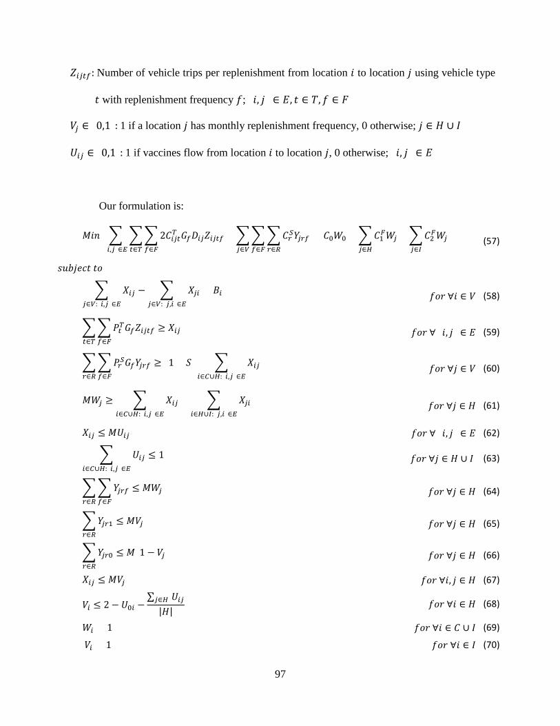
The objective function (57) consists of three terms: Annual round-trip transportation cost,

annual storage cost and annual facility cost. Constraint (58) is a conservation of flow equation,

where the inbound flow to a hub facility is equal to its outbound flow and the inbound flow to a

clinic is equal to its total demand. Constraint (59) ensures that if an edge representing

transportation between two locations is used, there are sufficient trips during each replenishment

using the selected vehicle to transport the total volume of vaccines required to be transported

along the edge. Constraint (60) ensures that a facility is able to have enough capacity (number of

storage devices) to store the total amount of vaccines before the next replenishment (including

any buffer stock). Constraint (61) states that if a facility is closed, the inbound flow to the facility

and outbound flow from the facility is 0. Constraint (62) states that if an edge is not used, there is

no flow on the edge. Constraint (63) ensures that each hub and clinic has at most one inflow.

Constraint (64) allows a facility to have storage devices only when a facility is open. Constraints

(65) and (66) stipulate that the 𝑌𝑌𝑖𝑖𝑟𝑟𝑓𝑓 variable has the appropriate value corresponding to the

selected replenishment frequency at facility 𝑗𝑗. Constraint (67) states that the trip or replenishment

frequency at a hub that is supplied by another hub is once a month. Constraint (68) guarantees

that a hub that is supplied by the center gets replenished once every quarter. Note that the

quantity ∑ 𝑈𝑈𝑖𝑖𝑖𝑖𝑖𝑖∈𝐻𝐻

|𝐻𝐻| is a positive fraction between 0 and 1 so that if there is shipment from the

98

central store to hub 𝑖𝑖, then 𝑉𝑉𝑖𝑖 must be equal to zero (quarterly replenishments); otherwise it could

be 0 or 1. Constraint (69) ensures that the central distribution center and all local clinics are

open, while Constraint (70) ensures that all local clinics have monthly replenishments. Finally,

Constraint (71) states that the central distribution center must have a cold room.

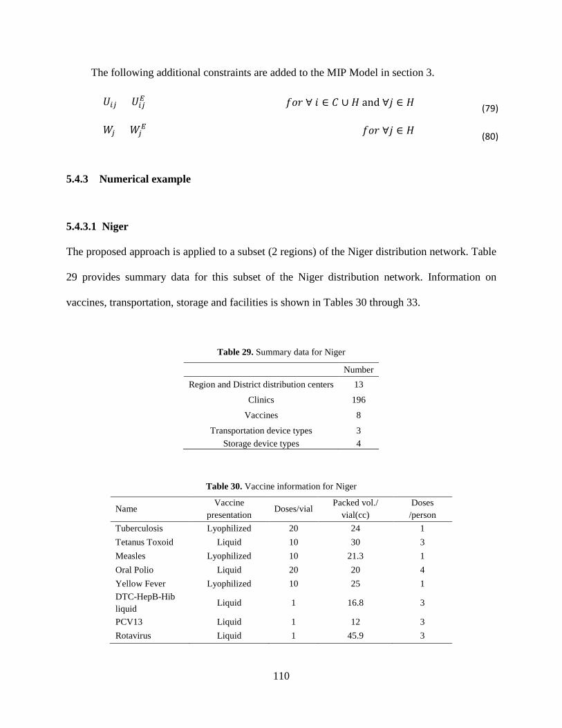
The above formulation can be used to solve the network problem optimally, but as the

problem size becomes bigger, the computational time increases exponentially. For example,

suppose there are three kinds of storage devices and three kinds of transportation vehicles, along

with five candidate hubs and 125 clinic locations. For this problem, the MIP formulation leads

to approximately 102,500 integer variables. If we increase the number of candidate hubs and

clinics by a factor of four (which would be quite representative of the structure in many

countries), the number of integer variables increases by a factor of 16 to approximately

1,627,000. Even if the computational effort is not directly proportional to the number of integer

variables, the additional computational time required to solve the model can be prohibitive. For

example, the largest problem we can solve with the MIP formulation has 210 locations including

13 candidate hubs. It takes 196 hours using IMB ILOG CPLEX 12.6 on a computer with an Intel

Xeon CPU E5450 3.00 GHz with 20.0 GB memory (also note that different combinations of

CPLEX parameters were evaluated before choosing the one that minimized computational time).

This problem represents only two of the eight regions in Niger. Many network problems have a

similar issue with dramatic increases in computational effort as the size of the problem gets

larger. Often, this issue is addressed by developing heuristics based on Lagrangian relaxation,

linear programming, or constructive methods, or by using so-called metaheuristics (Melo,

Nickel, & Saldanha-Da-Gama, 2009).

99

In the next section, we propose a metaheuristic that uses an evolutionary strategy (ES) to

obtain a good solution to the network problem in a reasonable amount of time.

5.4 EVOLUTIONARY STRATEGY ALGORITHM

5.4.1 Introduction

An Evolutionary Strategy (ES) is a population based algorithm that is related to genetic

algorithms, which were developed independently (Whitley, 1994) and have been used to solve

large network problems (Altiparmaka, F; Genb, M; Linb, L; Paksoy, T, 2006; H. Aytug , M.

Khouja & F. E. Vergara, 2003; Altiparmak, F; Gen, M; Lin, L; Karaoglan, I, 2009). ES is based

on the work of Rechenberg and Schwefel (Schwefel, 1975).

An ES can be a good candidate for solving the vaccine distribution network design

problem based on the problem’s characteristics and its likely optimal network structure: (a) most

clinics will tend to be supplied from the nearest open hub, (b) the number of candidate hubs is

relatively small; e.g., Niger has 40 candidate hubs even though there are 644 clinic locations, and

(c) the optimal network has a tree structure which is not very deep and its branches can be

clustered. Fact (a) implies that the ES does not need to have all connection information for the

entire network and that the network structure from the central distribution center to the hubs is

more critical (this is discussed in more detail later). Facts (a) and (b) permit the design of a

simple ES representation that facilitates ES operations such as crossover and mutation, and can

decrease the evaluation time of a candidate solution. Fact (c) is a good feature to have for a

100

population based method such as ES because the ES operations can be effective at finding

improved solutions in successive iterations of the algorithm.

There are two types of ES: (𝜇𝜇 + 𝜆𝜆)-ES and (𝜇𝜇, 𝜆𝜆)-ES. The (𝜇𝜇, 𝜆𝜆)-ES is closer to the

canonical genetic algorithm, where 𝜇𝜇 parents produce 𝜆𝜆 offspring and only the best 𝜇𝜇 of the

𝜆𝜆 offspring replace the 𝜇𝜇 parents (𝜇𝜇 < 𝜆𝜆). On the other hand, in the (𝜇𝜇 + 𝜆𝜆)-ES, 𝜇𝜇 parents

produce 𝜆𝜆 offspring, and the population is then reduced again to 𝜇𝜇 parents by selecting the best

solutions from among both the parents and offspring (Whitley, 1994). In this chapter, a (𝜇𝜇 +

𝜆𝜆)-ES is used to apply high selective pressure. Goldberg and Deb have shown that replacing the

worst member of the population tends to produce higher selective pressure (Goldberg & Deb,

1991).

One of the reasons for long computation times for the MIP model is that the vaccine

volumes handled at the hubs cannot be fixed before the network structure is set. In the ES, a

chromosome decides the network structure from the central storage location to the hubs and the

local clinics are automatically assigned to the nearest open hub to then complete the entire

network. Throughout the network, the amount of vaccine that must be handled at each hub

location is decided and then appropriate transportation and storage devices are selected. Note that

the best possible result found using the ES representation is not guaranteed to be an optimal

solution since the local clinics do not necessarily have to be connected to the nearest open hubs.

This is because clinic to hub assignments that result in more travel distance may result in lower

overall cost of storage device costs. For example, if Hub A can eliminate one storage device by

not servicing one of its clinics and there is another hub, say Hub B, which has sufficient storage

space to supply the clinic which was supplied by Hub A. If the cost of doing this from Hub B is

lower than the cost of using one more storage device at Hub A, then the local clinic (which was

101

supplied by Hub A) can now be supplied by Hub B. However, it is reasonable that in an optimal

solution one could expect many of the local clinics to be connected to the nearest open hubs.

Therefore, even though the ES does not guarantee that it can solve the network problem

optimally, it can hopefully produce a very good solution. In addition, if we fix the portion of the

network structure that does not include the clinics, solving the problem is much easier and

computation times decrease dramatically because the number of clinics greatly exceeds the

number of candidate hub locations.

In this section, an evolutionary strategy is introduced in order to address the

computational problems associated with the MIP formulation of the vaccine network problems,

and numerical examples are presented to illustrate the approach and demonstrate its

effectiveness.

5.4.2 An ES for vaccine supply chain network design

5.4.2.1 The ES procedure

Figure 14 shows the flow of the ES. The upper part shows the ES procedures and the lower part

presents the post processing that occurs after terminating the ES. The ES basically follows a

Genitor (𝜇𝜇 + 𝜆𝜆) strategy. However, here we initially generate a population of size 2𝜇𝜇 and then

choose the best 𝜇𝜇 of these for higher selective pressure. Moreover, we continue to maintain a

population of size 𝜇𝜇 until termination, where the members are ranked at the beginning of each

iteration in descending order of their fitness/performance. In the crossover step we select one

parent at random from the population and another from the top α1% of the population. As we

will explain, because of how the crossover is performed the number of offspring chromosomes

produced (λ1) is not the same at each iteration. Similar to crossover, in the mutation step we elect

102

one chromosome at random from the population and another from the top α2% of the population,

these generate λ2=2 new chromosomes. The 𝜆𝜆 = 𝜆𝜆1 + 𝜆𝜆2 new offspring generated at the iteration

are then added to the existing µ members and the entire population is then re-ranked and reduced

to a new set of µ members by eliminating the ones at the bottom. This completes one iteration

and we repeat the process with the new population. The process is terminated either when there

is no change in the population’s best α3% of chromosomes over T successive iterations or after

Tmax iterations. In the post-processing step we then solve the MIP with the central-to-hub

structure fixed according to the best chromosome in order to obtain the assignment of clinics to

hubs.

2 x μ population members produced select

μ members produce λ1(not fixed) offspring

- Select 2 parents, one from the μ members of the population, the other from top α

1% of the population.

- Fitness value is assigned according to fitness-function based rank

Initialize

Evaluate

Select

Crossover

Mutate

Evaluate

Terminate

Update Offspring replace existing members in the population if they are better

Evaluate λ (=λ1+λ

2) offspring

Perform mutation by randomly selecting one population member and choosing the other from the top α

2 % of the population to produce λ

2 offspring

Solve MIP

Terminate the ES either after Tmax

iterations, or if there is no improvement over T successive iterations

No

Yes

Solve MIP with fixed central-to-hubs structure (network) of the best chromosome from the ES to determine the hubs-to-clinics structure (network) optimally

Evolutionary Strategy (Genitor

(μ+λ)- ES)

Post Processing

Figure 14. Evolution strategy for the network problem

103

The solution representation and initialization are now described in more detail. A

matrix-based representation, which falls into the category of edge-based representations, is used

to represent the solutions. A chromosome is represented by an (𝑛𝑛 + 1) × 𝑛𝑛 matrix, where 𝑛𝑛 is

the number of hubs. Rows in the matrix correspond to the outbound flow from hubs and

columns to the inbound flow into hubs. That is, 𝑀𝑀𝑖𝑖𝑖𝑖 = 1 implies that hub 𝑖𝑖 supplies hub 𝑗𝑗, and

𝑀𝑀𝑖𝑖𝑖𝑖 = 0 implies that hub 𝑖𝑖 and hub 𝑗𝑗 are not connected, where 𝑀𝑀𝑖𝑖𝑖𝑖 is an element of the matrix in

row 𝑖𝑖 and column 𝑗𝑗. The first row represents the central distribution center. Figure 15 shows

examples of two chromosomes for 𝑛𝑛 = 6.

Figure 15. Chromosome examples

Note that since each location can be supplied by exactly one location, each column sum is

less than or equal to one.

For initializing a new chromosome, we use the following steps:

Step 1. The values of the elements in the first row are decided randomly, with each

column having a probability 𝑝𝑝1 of being selected and assigned a value of 1. This fixes which

hubs are supplied from the central distribution center. If hub 𝑖𝑖 is supplied from the central store,

it is an open hub and 𝑖𝑖 is inserted into the open hub set (= 𝑂𝑂). Other hubs that are not in 𝑂𝑂 are

assigned to the complementary set 𝐿𝐿.

104

Step 2. Next, wechoose an open hub, say 𝑗𝑗 ∈ 𝑂𝑂, update 𝑂𝑂 = 𝑂𝑂\{𝑗𝑗}, and randomly decide

whether 𝑗𝑗 supplies other hubs or not, where 𝑝𝑝2 is the probability that hub 𝑗𝑗 supplies other hubs

and (1-𝑝𝑝2) the probability that it does not. If 𝑗𝑗 is selected to supply other hubs, then a hub 𝑘𝑘 ∈ 𝐿𝐿

is selected to be supplied from 𝑗𝑗 with probability 𝑝𝑝3 and we update 𝑂𝑂 = 𝑂𝑂 ∪ {𝑘𝑘} and 𝐿𝐿 = 𝐿𝐿\{𝑘𝑘}

with each selection k.

Step 3. Repeat step 2 until 𝑂𝑂 = ∅.

5.4.2.2 Evaluation

A chromosome c has network information from the central store to the hubs, but does not have

information from hubs to clinics. Therefore, for evaluation of a chromosome, each clinic is

temporarily assigned to the nearest open hub and the flows into each hub are determined. Based

on the flows into each location, the transportation volume along each connected arc and the

storage volume at each open facility are decided across the entire network. This is because once

the flows are fixed, the demand (or volume of vaccine to be stored) at each location is also

known. Based on this volume, we know the storage and transportation volumes required at each

node and along each arc that is used, respectively. Once these volumes are fixed, the

performance of the chromosome(= 𝐸𝐸(𝑐𝑐)) is evaluated as follows:

𝐸𝐸(𝑐𝑐) = � 2𝐷𝐷𝑖𝑖𝑖𝑖 min𝑡𝑡∈𝑇𝑇,𝑓𝑓∈𝐹𝐹

{𝐶𝐶𝑖𝑖𝑡𝑡𝑓𝑓𝑇𝑇 𝐺𝐺𝑓𝑓 �𝑋𝑋𝑖𝑖𝑖𝑖𝑃𝑃𝑡𝑡𝑇𝑇𝐺𝐺𝑓𝑓

�}(𝑖𝑖,𝑖𝑖)∈𝐸𝐸

+ � min𝑟𝑟∈𝑅𝑅,𝑓𝑓∈𝐹𝐹

{𝐶𝐶𝑟𝑟𝑆𝑆 �(1 + 𝑆𝑆)∑ 𝑋𝑋𝑖𝑖𝑖𝑖𝑖𝑖∈𝐶𝐶∪𝐻𝐻:(𝑖𝑖,𝑖𝑖)∈ 𝐸𝐸

𝑃𝑃𝑟𝑟𝑆𝑆𝐺𝐺𝑓𝑓�}

𝑖𝑖∈𝑉𝑉

+ 𝐶𝐶0𝑊𝑊0

+ �𝐶𝐶1𝐹𝐹𝑊𝑊𝑖𝑖𝑖𝑖∈𝐻𝐻

+ �𝐶𝐶2𝐹𝐹𝑊𝑊𝑖𝑖𝑖𝑖∈𝐼𝐼

(78)

The first term, where the lowest cost transportation vehicle and the shipping frequency

are decided, determines the annual transportation cost. The second, where the lowest cost storage

device and replenishment frequency are decided, determines the total annual storage cost, and

105

the last term determines the annual facility cost. Note that the network structure determines the

values of Wj and Uij.

5.4.2.3 Selection

After a chromosome is evaluated, a fitness value is assigned based on the chromosome’s rank in

the population. In the selection step for crossover, two parents are selected: one is chosen

randomly from the whole population and the other is chosen randomly from the top 𝛼𝛼1% of the

population, based on the fitness rank. The reason why we choose one parent from the top 𝛼𝛼1% is

to apply higher selective pressure. Similarly, two chromosomes are also selected for mutation:

one is randomly chosen from the top 𝛼𝛼2% of the population and the other is randomly chosen

from the entire population.

5.4.2.4 Crossover

A 1-point crossover is performed between the two parents, where the crossover point is

randomly selected. Swapping the fragments occurs only in the first row within the column and

the other 𝑛𝑛 rows follow the crossover from the first rows. That is, the crossover point divides the

network tree into two sub-trees and then sub-trees are swapped between the two parents. For

example, in Figure 16, if chromosomes 1 and 2 at the top are swapped between column 3 and 4,

the crossover results are shown. In this example there is no duplication of hubs and both

offspring are feasible, but in general, this need not be the case. If redundant hubs exist across the

two sub-trees, we might have a hub that is supplied from two upper level facilities (or a cycle

may occur). For instance, in Figure 17, if node 2 in chromosome 1 supplies nodes 1 and 4 instead

of nodes 1 and 3, then one of the offspring, chromosome 1′, has a cycle, where node 4 is

supplied by both the central node and node 2. Node 4 can select only one supply node: either the

106

central node or node 2 as shown in the right hand side of the figure. Thus, chromosome 1′ and

chromosome 2 produce three offspring. Note that there might be several redundant hubs when

crossover is performed and because every redundant hub increases the number of offspring by a

factor of 2. This is why 𝜆𝜆1is not fixed. If there are no redundant hubs, the two parents produce

two offspring (𝜆𝜆1 = 2), but if there are in general, 𝑛𝑛(≥ 1) redundant hubs in a child chromosome

after the crossover, it is replaced by 2 × 𝑛𝑛 new child chormosomes.

Figure 16. Crossover example

107

Figure 17. Example of handling a redundant hub in crossover

5.4.2.5 Mutation

Mutation occurs with probability 𝑝𝑝𝑚𝑚 at every iteration. Two chromosomes are selected for

mutation: one from the top 𝛼𝛼2% of the population and the other randomly selected from the

entire population. There are three options for mutation: (1) eliminating a hub, (2) adding a hub,

and (3) exchanging hubs. Each type of mutation has the same probability of occurring. Figure 18

illustrates these mutations. If option (1) is selected, a hub selected randomly from the open hubs

is removed from the network. If a hub (say, Hub A) is removed, then any hubs supplied by Hub

A are now supplied directly from the location that supplied Hub A. If option (2) is chosen, a hub

(say, Hub B) among the closed hubs and a hub (say, Hub C) among the open hubs (including the

central distribution center) are selected, and Hub C and Hub B are connected. In option (3), two

hubs among the open hubs are selected and their positions are exchanged.

108

Figure 18. Mutation

5.4.2.6 Termination and optimization

After evaluation, if no change is observed in the top 𝛼𝛼3% of the population over 𝑇𝑇 successive

iterations, or we have reached our iteration limit of Tmax, the algorithm is terminated. Although

the best chromosome has the minimum cost only the network structure from the central location

to the hubs is considered for optimization, and the network from the hubs and the local clinics is

not optimized. However, if the network from the central location to the hubs is fixed, assigning

the local clinics to the hubs optimally is relatively easy. This is done by solving an MIP problem

with the upper level of the network structure being fixed to the one that the ES produces.

Consider an open location i∈C∪H and link i-j, j∈H along which vaccines flow, as determined by

the ES and define:

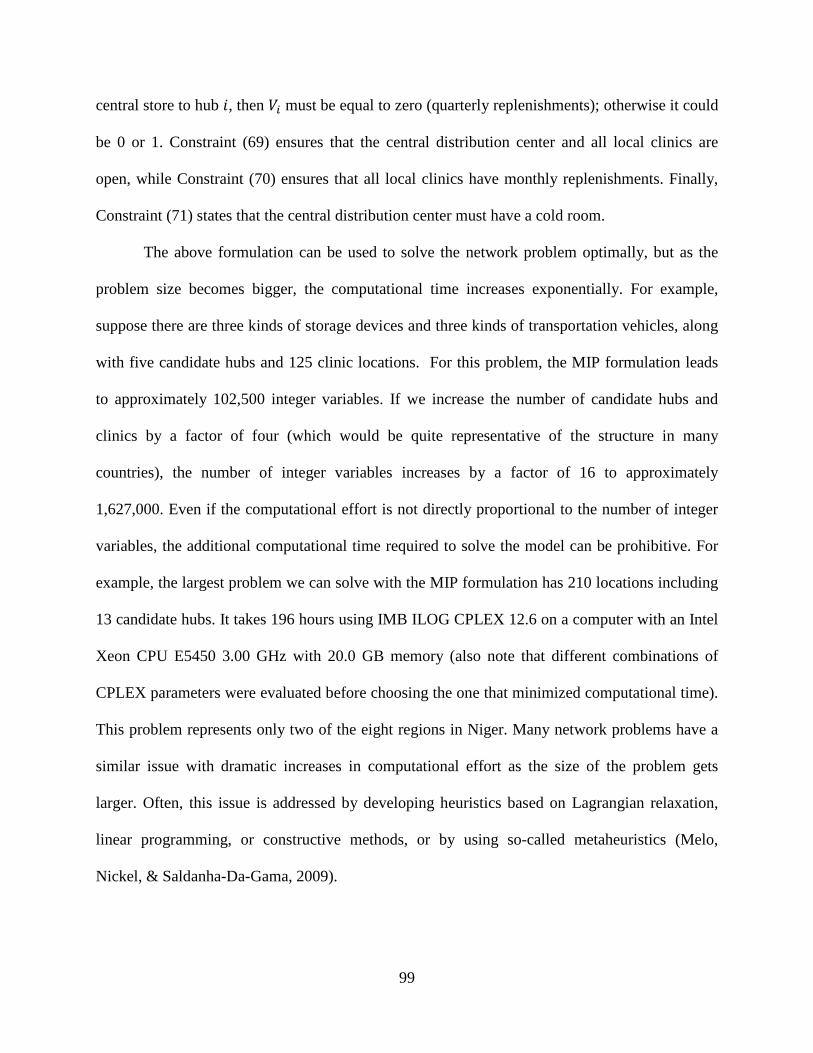
𝑊𝑊𝑖𝑖𝐸𝐸 ∈ {0,1}: 1 if location 𝑗𝑗 is open, 0 otherwise; 𝑗𝑗 ∈ 𝐻𝐻

𝑈𝑈𝑖𝑖𝑖𝑖𝐸𝐸 ∈ {0,1}: 1 if vaccines flow from location 𝑖𝑖 to location 𝑗𝑗, 0 otherwise; 𝑖𝑖 ∈ 𝐶𝐶 ∪ 𝐻𝐻 𝑀𝑀𝑛𝑛𝑑𝑑 𝑗𝑗 ∈ 𝐻𝐻

109

The following additional constraints are added to the MIP Model in section 3.

𝑈𝑈𝑖𝑖𝑖𝑖 = 𝑈𝑈𝑖𝑖𝑖𝑖𝐸𝐸 𝑓𝑓𝑓𝑓𝑓𝑓 ∀ 𝑖𝑖 ∈ 𝐶𝐶 ∪ 𝐻𝐻 and ∀𝑗𝑗 ∈ 𝐻𝐻 (79)

𝑊𝑊𝑖𝑖 = 𝑊𝑊𝑖𝑖𝐸𝐸 𝑓𝑓𝑓𝑓𝑓𝑓 ∀𝑗𝑗 ∈ 𝐻𝐻 (80)


5.4.3.1 Niger

The proposed approach is applied to a subset (2 regions) of the Niger distribution network. Table

29 provides summary data for this subset of the Niger distribution network. Information on

vaccines, transportation, storage and facilities is shown in Tables 30 through 33.

Table 29. Summary data for Niger

Number Region and District distribution centers 13

Clinics 196

Vaccines 8

Transportation device types 3 Storage device types 4

Table 30. Vaccine information for Niger

Name Vaccine

presentation Doses/vial


Doses /person

Tuberculosis Lyophilized 20 24 1 Tetanus Toxoid Liquid 10 30 3 Measles Lyophilized 10 21.3 1 Oral Polio Liquid 20 20 4 Yellow Fever Lyophilized 10 25 1 DTC-HepB-Hib liquid

Liquid 1 16.8 3

PCV13 Liquid 1 12 3 Rotavirus Liquid 1 45.9 3

110

Table 31. Transportation information for Niger

Vehicle Type Capacity (L) Cost ($/km)

Cold truck 9,293 0.97 4x4 Truck 172 0.54 Motorbike 5 0.23

Table 32. Storage information for Niger

Device Type Capacity (L) Cost ($/year) Cold room 18,000 8,116

Regional level device 1,843 1,582 District level device 76 600 Clinic level device 35 596

Table 33. Facility information for Niger

Facility type Cost ($/year) Central 40,000 Region 13,000

District/Hub 4,500 Clinic 800

Note that capacity and cost of transportation vehicles and storage devices at a particular

level are weighted average values based on the equipment currently used at that level. For

example, if there are 1,000 units of a 40-liter storage device and 600 units of a 20-liter storage

device across the clinic level, the storage device assigned to the clinic level is assigned a capacity

of 32.5 (=(1000×40+600×20)/1600) liters. This procedure is in order to simplify the problem. If

we were to include every currently used vehicle and device type in the model as an option this

would dramatically increase the computational effort. Facility cost is estimated based on labor

and building operation costs.

111

This subnetwork has one central distribution center, along with 13 regional and district

distribution centers, which are potential hubs. Table 6 provides three different network design

results for the network. The first is the cost of the original network with the currently assigned

vehicles and storage devices for the routes and locations, respectively. The second still uses the

original network structure, that is, all the facilities are open and vaccines are distributed using the

current routes, but vehicles and storage devices are optimally assigned to each route and each

facility. The last is the network that is optimized for structure as well as devices using the

original MIP in Section 5.3. Figure 19 shows the resulting graphs for each network. Black lines

imply the use of cold trucks, orange lines correspond to 4×4 trucks, and blue lines to motorbikes.

Table 34. Network cost for Niger

Network Total cost Transportation cost

Storage cost

Facility cost

Computation time

Original Network 961,014 394,852 293,862 272,300 Original Network with

optimized devices 660,330 140,064 247,966 272,300 ≤ 1 sec

Optimized Network 605,193 135,107 237,286 232,800 196 hours

Original Network Original Network with optimized devices

Optimized Network

Figure 19. Network graphs for Niger

112

The annual cost of the original network is $961,014. Maintaining the original network

structure but optimizing the transportation vehicles and storage devices used reduces the costs to

$660,330. Thus, if we assign the transportation vehicles and storage devices to the facilities more

appropriately, a cost savings of about 30% is possible for this subset of the Niger network. These

savings come mostly from reduced transportation costs. If we solve this network problem

optimally using the MIP described in Section 5.3, the total cost is $605,193, which is almost

another 10% in additional savings and around 37% in savings from the original network.

However, the computation time required to solve the problem optimally was 196 hours. The

computational experiments were done using a computer with an Intel Xeon CPU E5450 3.00

GHz processor and 20.0 GB of RAM. Since the whole Niger network has 40 candidate hubs and

644 clinics, solving the entire network with this computer in a reasonable amount of time is not

possible.

This same problem was also solved using the ES to fix the central-to-hub network

combined with the MIP post processing to get the clinic to hub assignment. Table 35 shows the

results of the ES + post processing for six different values of µ (the population size), where each

of the six runs has 30 replications, each with different random number seeds. The ES input

parameters are shown in Table 36. Note that extensive pilot tests were run for a range of

parameter values and these values were chosen because the pilot testing indicated that this set

performed best. The mean, standard deviation and minimum values across these 30 replicates

along with the run times are reported. We also report the number of replicates in which the best

solution found by the ES is also the optimal solution of the MIP (=Frequency of optimum).

113

Table 35. ES results

Population 10 25 50 100 300 600 Min 605,193 605,193 605,193 605,193 605,193 605,193 Avg 606,910 606,595 606,347 606,030 605,901 605,946 SD 1,807 972 760 424 433 311

Frequency of optimum 2 1 1 3 6 2

Run time for 30 replications (sec)

1,114 1,122 1,383 1,744 1,957 2,354

Table 36. ES parameter settings

Parameter Value 𝜇𝜇 (10, 25, 50, 100, 300, 600) 𝑝𝑝𝑚𝑚 100% 𝛼𝛼1 10 𝛼𝛼2 20 𝛼𝛼3 50 𝜆𝜆2 2 𝑝𝑝1 20% 𝑝𝑝2 40% 𝑝𝑝3 20% 𝑇𝑇 100

𝑇𝑇𝑚𝑚𝑚𝑚𝑚𝑚 1000

Figure 20. ES results for Niger

With 𝜇𝜇 ≥ 100, the ES provides stable results (Figure 20) in terms of the average quality

of the best solution in the population. An analysis of variance indicates that there is no

114

significant difference between the solutions found by population sizes over 100 and the t-tests

between different populations indicate that the poulation sizes that are over 100 have a

significantly different average than those with population sizes less than 100. Thus, a population

size of 100 or more is preferable although there is no advantage to making it larger than 100. For

𝜇𝜇 ≥ 100, the value of the solution found is on average about $606,000, which is 0.14% higher

than the cost found by the MIP. Recall that the ES does not assign clinics to hubs optimally, and

therefore the best solution found by the ES is not guaranteed to be the optimal one found by

solving the MIP. In this example, each experimental run has 30 replications and in all cases the

minimum cost found by at least one of the replicates was equal to the optimal value of $605,193

from the MIP. Each run takes 15 to 30 minutes to run 30 replications, which is a huge decrease

in computation time compared to directly solving the original MIP.

Since the clinics are assigned to the nearest hub in the ES evaluation step, the best ES

solution is not necessarily the same as the optimal solution of the MIP. Before deciding the final

network, replications are required to get the best solution. From the example of this section,

regardless of the size of the population, the minimum solution across 30 replications was the

same in all cases. So instead of increasing the size of the population, increasing the number of

replication is a better strategy.

5.4.3.2 Additional examples

In order to further evaluate the performance of the ES, similar experiments, using a

population size of 100 for the ES, are performed for a subset of the networks found in three

countries: Benin, Country A, and Country B. (Note that we use Country A and B instead of the

actual country names because the Ministries of Health in those countries did not give us

permission to use their country names – while the Ministries of Health in Benin and Niger did

115

give permission to use their names.) The parameter settings for the ES are the same as with

Niger. Table 37 provides summary data for the network subsets of these three countries. The

results are shown in table 38. In the Benin and Country A cases, the ES consistently found the

optimal solutions. The average ES cost for Country B is 213,692, which is 0.1% more than the

optimal solution.

Table 37. Summary data for Benin, Country A, and Country B

Benin Country A Country B Region and District distribution centers 13 10 11

Clinics 114 106 130 Vaccines 8 7 7

Transportation device types 3 3 3 Storage device types 4 4 4

Table 38. Results for Benin, Country A, and Country B

Benin Country A Country B Original Network 158,330 771,290 294,739

Original Network with optimized devices 157,052 771,290 291,103

Optimized Network 142,543 593,326 213,422 ES result (average of 30 replications) 142,5431) 593,3261) 213,6921) ES Run time for 30 replications (sec) 460 319 630

1) These instances are relatively small, so the ES yields the same result for all 30 replications.

These smaller test problems have been used to demonstrate the effectiveness of the ES

since the optimal solution can be determined for these smaller problems. However, the ES was

created to find solutions to larger problems which the MIP model cannot solve in a reasonable

amount of time. Thus, we now examine country-level problems for four countries, which the

MIP model cannot solve in real time: Niger, Benin, Country A, and Country B. Table 39

provides summary data for these four countries. The parameter settings are the same as with the

116

previous Niger example except that the iteration limit is now set to 5000 (as opposed to 1000).

The results are shown in Table 40.

Table 39. Number of locations for Niger, Benin, Country A, and Country B

Niger Benin Country A Country B

Region and District distribution centers 41 87 141 81

Clinics 644 658 2733 851

Table 40. Country level results for Niger Benin, Country A, and Country B

Niger Benin Country A Country B

Original Network (A) 2,989,490 791,164 11,182,800 6,987,500

Original Network with optimized devices 2,054,260 788,913 11,150,900 6,647,460

Best ES result (B) 1,903,500 718,898 8,710,000 5,414,090

Average 1,907,716 721,146 8,730,283 5,425,201

Standard deviation 4,057 1,294 11,870 17,900

Savings ((A-B)/A×100%) 36% 9% 22% 23%

ES Run time for 30 replications 3.7 hours 5.9 hours 30.1 hours 21.5 hours

5.4.4 Discussion

The ES can obtain excellent solutions to the network problem in a very reasonable amount of

computational time. Given that we cannot solve these large problems optimally in a reasonable

amount of time, it is not possible to objectively evaluate the quality of the ES solution to these

problems. However, since the ES did well on smaller examples where we could indeed verify

optimality, it is reasonable to conclude that that these solutions are likely to be very good. This

117

performance may be explained in terms of the following structural features of the vaccine

distribution network.

1. A vaccine network does not have many candidate hubs relative to the total number of

nodes in the network because the vast majority of nodes correspond to clinic locations.

2. Clinics are often assigned to the nearest open hub in an optimal solution.

3. The optimal network is not very deep.

4. An optimal network has a tree structure.

In addition, the following design features of the ES help it to find a good solution in a

reasonable amount of time.

1. The ES constructs the network structure only from a central distribution center to hubs.

2. Clinics are heuristically assigned to the nearest open hub in the ES (although we allow

ourselves the option of changing this in the post-processing step).

3. The crossover occurs between hubs supplied by a central distribution center.

5.5 SENSITIVITY ANALYSIS

The vaccine distribution network has three associated cost parameters - storage, transportation

and facility costs - that are calculated based on storage device cost per year, transportation cost

per trip and facility cost per year, respectively. They are fixed values in the model but in practice

it might not be possible to ascertain exact values for these. In order to investigate the effects of

cost variation on the network structure, we perform a sensitivity analysis around these cost

estimates. One cost element at a time is perturbed, while the other two other are fixed. Each cost

element is altered from 10% to 1,000% of the baseline value (with the other two maintained at

118

their baseline values). Subsets of the Niger, Benin, Country A and Country B vaccine

distribution networks are used with the MIP. For Niger a larger problem with 2 regions, which is

used in section 5.4.3.1,is also considered, but with the ES (which will likely provide at least a

near-optimal solution), since running the MIP for this several times would take an inordinate

amount of time. Since the MIP can provide the optimal network, we can readily observe the

impact of the changes. Table 41 shows the number of candidate hubs and clinics in the four

countries.

Table 41. Country information for sensitivity analysis

Country Niger Benin Country B Country A Number of candidate hubs 5 13 11 10

Number. of clinics 86 114 130 106

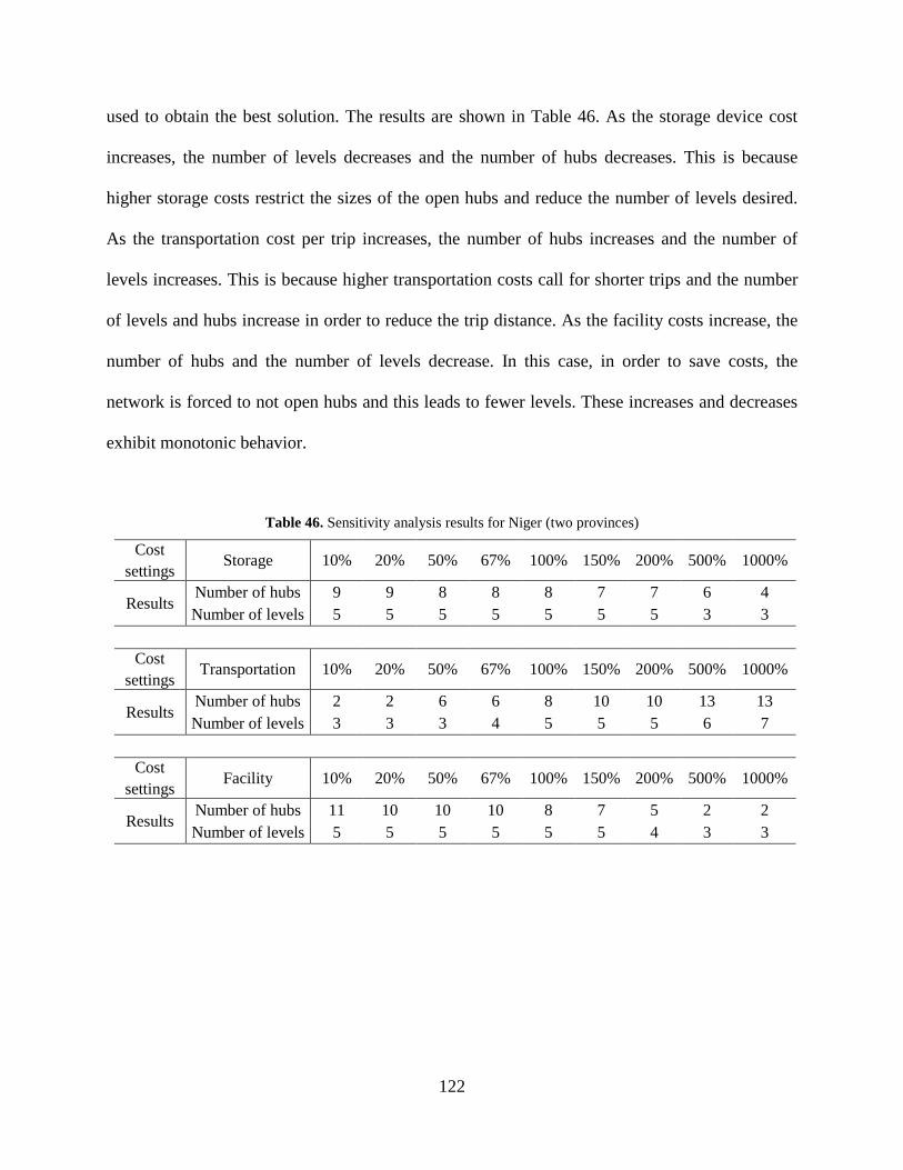
Our interest is to study how the network changes according to how the costs vary.

Therefore, we focus on the number of open hubs, the number of hubs supplied by a central

distribution center and the number of levels.

5.5.1 Results

Table 42 shows the results of the sensitivity analysis for Niger (one district) which are obtained

via the MIP. It indicates that changes in storage device costs have no effect on the network

design but changes in transportation and facility cost can alter the network structure. As the

transportation cost per trip increases from 10% to 1000% of its nominal value, the number of

hubs increases. In the situation where the transportation cost is low, frequent trips are preferred

and fewer hubs are open. When transportation costs are high, opening more hubs can reduce

119

costs by decreasing the number of trips required. The effect of changes in facility cost per year

has an opposite effect to transportation cost changes. Higher facility costs decrease the number

of open hubs (with higher transportation costs) and lower facility costs increase the number of

open hubs (with lower transportation costs). Tables 43-45 show the sensitivity analysis results

for subsets of the Benin, Country B and Country A networks that were considered. These results

show trends similar to those obtained for Niger.

Table 42. Sensitivity analysis results for Niger (Dosso Province)

Cost Setting Storage 10% 20% 50% 67% 100% 150% 200% 500% 1000%

Results Number of hubs 3 3 3 3 3 3 3 3 3 Number of levels 3 3 3 3 3 3 3 3 3

Cost setting Transportation 10% 20% 50% 67% 100% 150% 200% 500% 1000%


Cost setting Facility 10% 20% 50% 67% 100% 150% 200% 500% 1000%


Table 43. Sensitivity analysis results for Benin

Cost settings Storage 10% 20% 50% 67% 100% 150% 200% 500% 1000%


Cost settings Transportation 10% 20% 50% 67% 100% 150% 200% 500% 1000%


Cost settings Facility 10% 20% 50% 67% 100% 150% 200% 500% 1000%


120

Table 44. Sensitivity analysis results for Country B

Cost settings Storage 10% 20% 50% 67% 100% 150% 200% 500% 1000%


Cost

settings Transportation 10% 20% 50% 67% 100% 150% 200% 500% 1000%




Table 45. Sensitivity analysis results for Country A

Cost settings

Storage 10% 20% 50% 67% 100% 150% 200% 500% 1000%

Results

Number of hubs 2 2 2 2 2 2 2 2 2 Number of levels 3 3 3 3 3 3 3 3 3

Cost settings

Transportation 10% 20% 50% 67% 100% 150% 200% 500% 1000%

Results


Cost settings

Facility 10% 20% 50% 67% 100% 150% 200% 500% 1000%

Results


The Niger network instance includes only one of its eight districts, so the three level

network is optimal even though the cost factors are altered. This makes it impossible to see any

changes in the network’s depth. In order to examine this further, we also study a problem

instance with two districts of Niger, which has 13 candidate hubs and 196 clinics. This instance

can be solved by the MIP but it takes around 8 hours to get the optimal solution, so the ES is

121

used to obtain the best solution. The results are shown in Table 46. As the storage device cost

increases, the number of levels decreases and the number of hubs decreases. This is because

higher storage costs restrict the sizes of the open hubs and reduce the number of levels desired.

As the transportation cost per trip increases, the number of hubs increases and the number of

levels increases. This is because higher transportation costs call for shorter trips and the number

of levels and hubs increase in order to reduce the trip distance. As the facility costs increase, the

number of hubs and the number of levels decrease. In this case, in order to save costs, the

network is forced to not open hubs and this leads to fewer levels. These increases and decreases

exhibit monotonic behavior.

Table 46. Sensitivity analysis results for Niger (two provinces)

Cost settings

Storage 10% 20% 50% 67% 100% 150% 200% 500% 1000%


Cost settings

Transportation 10% 20% 50% 67% 100% 150% 200% 500% 1000%




122

5.6 APPLYING A LOOPING FACTOR

5.6.1 Introduction

The current model assumes that a vaccine transportation vehicle visits only one place and returns

to the original point of departure. In practice, the vehicle may visit several locations during one

trip as long as it has enough capacity to carry all required vaccines. In order to add travel routes

between the central warehouse and hubs, vehicle routing constraints are required to be added to

the MIP model. However, the vehicle routing problem (VRP) is known to be an NP-Hard

problem. If we add VRP constraints into the current MIP model, it is not possible to solve it in

reasonable time for even small networks. So a two-step procedure is proposed for adding vehicle

routing. First, the network problem is solved using the MIP formulation or the ES procedure.

Once the network is fixed and the locations supplied by each of the hubs are decided, a vehicle

routing problem from each hub to its delivery locations is solved in order to optimize the travel

routes for that hub. Since there may be several hubs, the number of VRPs solved would be equal

to the number of hubs (plus one for the central warehouse).

The introduction of vehicle routing to the network problem leads to a decrease in the

transportation cost of the network because vehicles travel less than in a network where we

assume that all trips are point-to-point. Thus the network structure obtained from solving our

MIP (or by using the ES procedure) may be improved with the decreased transportation costs.

However, we do not actually know these costs until the network is fully solved. We therefore use

an estimate of the transportation cost for the optimization by applying a multiplicative looping

factor, which is computed as the ratio of the transportation cost with vehicle routing to the

transportation cost with all point-to-point travel. The transportation costs from the hub to each of

123

its delivery locations are then multiplied by this looping factor. The network design problem is

then solved again using these lower transportation costs. Figure 21 shows an example of the

looping factor calculation. Location D supplies locations 1-5. If a vehicle visits one place per

trip, the total distance is 132 (left side of Figure 21). When the vehicle has two big loops (right

side of Figure 21), the total distance is 93. Thus, the looping factor is calculated to be 0.705

(=93/132).

Figure 21. Looping factor example

Two issues arise when we solve the network design problem again. First, the central

distribution center and each of the hubs has its own looping factor, and the transportation costs

between a hub and its delivery locations are each multiplied by the hub’s looping factor. The

second issue is that the network structure obtained from the MIP or the ES procedure does not

use all routes, so only a few vehicle routing paths are available after solving the VRPs. Therefore

we assume that the network has representative looping factors depending on where the VRP

origin and destinations are. We group the VRP deliveries in the network into three categories –

central-to-hubs, hub-to-hubs and hub-to-clinics, and assume that there is a representative looping

124

factor corresponding to each of these categories.. Each representative looping factor is computed

as the average of all looping factors computed by the different VRPs within each category. For

example, consider the third category. Suppose there are five hubs with each one only supplying

clinics, and suppose their looping factors are found to be 0.35, 0.4, 0.38, 0.42 and 0.45. Then the

representative looping factor for hub-clinic deliveries is 0.4 (the average of these five values),

and the transportation cost for deliveries from any hub to any clinic is multiplied by 0.4.

5.6.2 Procedure

After finding an initial network structure using the MIP or the ES, looping factors are calculated.

However, once the network problem with the lower transportation costs is solved, the network

structure originally obtained might change. If this happens, a fresh set of looping factors are

computed for the new network and the procedure is repeated until there is no change in the

network. That is, it is an iterative procedure, as shown in Figure 22.

• STEP 0: Use the MIP or the ES to obtain the network structure {N}. Looping factors are

then obtained by solving VRPs resulting from {N} and the “true” cost of the network

(assuming we use these routes) is estimated as Z; this is done by multiplying each point-

to-point transportation cost in the network by its looping factor.

• STEP 1: The network problem is re-solved with these looping factors using the MIP or

the ES. If the structure of the new network {Nnew} is identical to {N} , we stop and the

current network structure is the best we can find. If the network structure has changed,

the VRPs resulting from this new structure {Nnew} are solved and new looping factors

obtained. The “true” cost of the network {Nnew} is estimated as Znew by multiplying the

125

original point-to-point transportation costs in the network by the appropriate looping

factors

• STEP 2: If Znew ≥ Z then the new network {Nnew} is not better and we stop with {N} as the

best structure we can find. If Znew < Z we have a better network, so we redefine

{N}≡{Nnew}, Z = Znew and return to Step 1.

Figure 22. Apply looping factors

5.6.3 Vehicle routing problem

There are many algorithms that have been developed for the VRP. Because the VRP is known to

be NP-Hard, many of these are heuristics. For this network problem, both an MIP formulation

and a heuristic method are used in this research. Since we need to solve many VRPs while

applying a looping factor, the MIP formulation is used for smaller problems where the VRPs can

be solved efficiently, while the heuristic is used when the VRPs take too much time to solve

optimally.

126

5.6.3.1 MIP Formulation

In this section, we describe a mathematical formulation corresponding to the VRPs that we solve.

This formulation considers the vehicle type to use for each loop and its capacity. It uses a binary

variable as a vehicle flow variable to show if there is travel between two locations using a

specific vehicle.

Notation

𝐶𝐶𝑖𝑖𝑖𝑖𝑡𝑡𝑇𝑇 ,𝑑𝑑𝑖𝑖,𝐵𝐵𝑖𝑖,𝑃𝑃𝑡𝑡𝑇𝑇 ,𝐶𝐶,𝐻𝐻, and 𝑇𝑇 follow the same notation as the network MIP. Define

𝑥𝑥𝑖𝑖𝑖𝑖𝑡𝑡 ∈ {0,1}: 1 if 𝑖𝑖 and 𝑗𝑗 are connected using vehicle type 𝑡𝑡; 0 otherwise.

𝑦𝑦𝑖𝑖𝑖𝑖𝑡𝑡 ∶ amount of vaccine transported from 𝑖𝑖 to 𝑗𝑗 using vehicle type 𝑡𝑡.

The following MIP is used to solve the VRP:

Min � � 𝐶𝐶𝑖𝑖𝑖𝑖𝑡𝑡𝑇𝑇 𝑥𝑥𝑖𝑖𝑖𝑖𝑡𝑡

𝑖𝑖,𝑖𝑖∈𝐶𝐶∪𝐻𝐻𝑡𝑡∈𝑇𝑇

(81)

𝑠𝑠𝑠𝑠𝑏𝑏𝑗𝑗𝑀𝑀𝑐𝑐𝑡𝑡 𝑡𝑡𝑓𝑓

� � 𝑥𝑥𝑖𝑖𝑖𝑖𝑡𝑡𝑖𝑖∈𝐶𝐶∪𝐻𝐻𝑡𝑡∈𝑇𝑇

= 1 for ∀𝑗𝑗 ∈ 𝐻𝐻 (82)

� 𝑥𝑥𝑖𝑖𝑖𝑖𝑘𝑘𝑖𝑖∈𝐶𝐶∪𝐻𝐻

− � 𝑥𝑥𝑖𝑖𝑖𝑖𝑡𝑡𝑖𝑖∈𝐶𝐶∪𝐻𝐻

= 0 for ∀𝑝𝑝 ∈ 𝐻𝐻,∀𝑡𝑡 ∈ 𝑇𝑇 (83)

� � 𝑦𝑦𝑖𝑖𝑖𝑖𝑡𝑡𝑖𝑖∈𝐶𝐶∪𝐻𝐻𝑡𝑡∈𝑇𝑇

−� � 𝑦𝑦𝑖𝑖𝑖𝑖𝑡𝑡𝑖𝑖∈𝐶𝐶∪𝐻𝐻𝑡𝑡∈𝑇𝑇

= 𝑑𝑑𝑖𝑖 for ∀𝑗𝑗 ∈ 𝐻𝐻 (84)

𝐵𝐵𝑖𝑖𝑥𝑥𝑖𝑖𝑖𝑖𝑡𝑡 ≤ 𝑦𝑦𝑖𝑖𝑖𝑖𝑡𝑡 ≤ 𝑃𝑃𝑡𝑡𝑇𝑇𝑥𝑥𝑖𝑖𝑖𝑖𝑘𝑘 for ∀𝑖𝑖, 𝑗𝑗 ∈ 𝐶𝐶 ∪ 𝐻𝐻, 𝑖𝑖 ≠ 𝑗𝑗,∀𝑡𝑡 ∈ 𝑇𝑇 (85)

𝑦𝑦𝑖𝑖𝑖𝑖𝑡𝑡 ≥ 0 for ∀𝑖𝑖, 𝑗𝑗 ∈ 𝐶𝐶 ∪ 𝐻𝐻, 𝑖𝑖 ≠ 𝑗𝑗,∀𝑡𝑡 ∈ 𝑇𝑇 (86)

𝑥𝑥𝑖𝑖𝑖𝑖𝑡𝑡 ∈ {0, 1} for ∀𝑖𝑖, 𝑗𝑗 ∈ 𝐶𝐶 ∪ 𝐻𝐻, 𝑖𝑖 ≠ 𝑗𝑗,∀𝑡𝑡 ∈ 𝑇𝑇 (87)

Constraints (82) and (83) ensure that a facility is visited exactly once and that if a vehicle

visits a location, it must also depart from it. Constraint (84) specifies that the difference between

127

the quantity of vaccines a vehicle carries before and after visiting a facility is equal to the

demand of that facility. Constraint (85) ensures that the vehicle capacity is never exceeded.

5.6.3.2 Heuristic method

Our heuristic uses a constructive method based on the algorithm of Clark and Wright (1964). In

this algorithm, point-to-point routes are combined to form a loop by choosing the routing path

that gives the largest transportation cost savings at each iteration until every location is linked.

For our network problem, vehicle type is considered when the savings on the route are

calculated. For checking if a route is feasible, both vehicle capacity and trip distance are

considered.

Modified Clark and Wright algorithm

Label the delivery locations as 1, 2, ..., n and label the origin as 0.

Determine the costs 𝐶𝐶𝑖𝑖𝑖𝑖𝑡𝑡𝑇𝑇 to travel between all pairs of delivery locations and between each

delivery location and the origin and for each vehicle type, i.e., for i=0, 1, .., n; j=0, ..., n and j≠i ,

t∈T

1. Calculate the savings 𝑆𝑆𝑖𝑖𝑖𝑖𝑘𝑘=𝐶𝐶𝑖𝑖0𝑡𝑡𝑇𝑇 + 𝐶𝐶0𝑖𝑖𝑡𝑡𝑇𝑇 − 𝐶𝐶𝑖𝑖𝑖𝑖𝑡𝑡𝑇𝑇 for all pairs of delivery -locations i,

j and vehicle types t (i=1, 2...n; j=1, 2...n; i=/ j, t∈T).

2. Order the savings, 𝑆𝑆𝑖𝑖𝑖𝑖𝑡𝑡, from largest to smallest.

3. Starting with the largest savings, do the following:

(a) If linking delivery locations i and j results in a feasible route, then add this link to

the route; if not, reject the link.

(b) Try the next savings in the list and repeat (a).

128

Checking for route feasibility

If the sum of vaccine volumes required at the delivery locations on the route is less than or equal

to the capacity of the vehicle and the total travel distance of the vehicle is less than or equal to

the maximum travel distance of the vehicle, the route is feasible; otherwise, the route is

infeasible.


Table 47 shows results from the Cotonou province of Benin when vehicle routing is considered.

This example is small enough that we can use the MIP to solve the network and also use an MIP

formulation to solve the VRPs. The original optimal value for the network {N} obtained after

solving the problem is 142,543. The corresponding VRPs are then solved and the looping factor

for the central distribution center to the hubs is computed as 0.4333 (i.e., 43.33%) while the

looping factor for the hub to the clinics is 0.4585 (i.e., 45.85%). There is no hub to hub

connection in this original network. The network cost with vehicle routing is estimated as

Z=138,810; this is obtained by multiplying the transportation costs at each route (edge) by its

looping factor. In particular, the transportation costs per km (𝐶𝐶𝑖𝑖𝑖𝑖𝑡𝑡𝑇𝑇 ) from the central distribution

center to each hub and from each hub to a clinic are multiplied by 0.4333 and 0.4585,

respectively.

Next, the MIP is solved again with transportation costs based on the above looping

factors and we obtain a new network {Nnew} with a cost of 138,393. After solving the associated

VRPs this new network yields values of 1.00 and 0.391 respectively for the looping factors for

central to hubs and hub to clinics each, and the true cost for this network {Nnew} with routing is

estimated as Znew =138,333. Since the network is changed and the cost has decreased

129

(138,333<138,810 (Table 47)), we perform a second iteration after resetting Z=138,333 and

{N}≡{Nnew}.

After the second iteration, the new network {Nnew} is different from {N} and the VRPs

yield new looping factors of 1.00 and 0.316. Since there is improvement in the network cost

(Znew= 137,494<138,333=Z (Table 47)), a third iteration is performed after resetting Z=137,494.

After the third iteration, the solution to the network design problem is the same as the one from

the previous iteration. Therefore, we stop here and accept this network structure with vehicle

routing as the final one. Table 48 also shows the results for the same problem using the heuristic

method for the VRPs instead of the MIP formulation. The iterations proceed in a similar fashion

but the final network is different with looping factors of 1.00 and 0.3533 and a final cost of

Z=137,831. The final network with the MIP VRP solver is little bit better than with the heuristic

VRP solver (137,474 <137,831), because the MIP VRP solver provided optimal VRP solutions.

Table 47. Results of applying a looping factor for Benin (MIP-MIP)

Initial Network Iteration 1 Iteration 2 Iteration 3 MIP Cost 142,543 138,393 138,171 137,494

Looping Factor (MIP)

C-H 43.33% 100.0% 100.0% 100.0% H-H - - - - H-I 45.85% 39.10% 31.60% 31.60%

Cost (Z) 138,810 138,333 137,494 137,494

Table 48. Results of applying a looping factor for Benin (MIP-Heuristic)

Initial Network Iteration 1 Iteration 2 Iteration 3 MIP Cost 142,543 138,753 138,419 137,831

Looping factor

(Heuristic)

C-H 43.33% 100% 100% 100% H-H - - - - H-I 50.64% 41.85% 35.33% 35.33%

Cost (Z) 139,106 138,539 137,831 137,831

130

Figure 23 shows the network structures at each iteration. As the iterations proceed, the

number of hubs decreases. This is because allowing vehicle routing reduces the transportation

cost substantially and this result is similar to the one obtained while conducting sensitivity

analysis on transportation costs.

Figure 23. Network structure at each iteration (MIP-MIP)

5.6.5 Discussion

If a vehicle has enough capacity, visiting several locations during a trip is reasonable. Actually,

this is common in practice. So solving a network assuming point-to-point trips can result in an

undesirable solution. In this section, we described how vehicle routing can be incorporated into

131

the network problem using looping factors. Here, three looping factors – central distribution

center to hubs, hub to hub, and hub to clinic - are used. This makes the simplifying assumption

that the transportation costs between all points at one level and all destinations at the next lower

level can be reduced by a similar percentage using delivery loops.

We cannot guarantee that the final network is optimal with vehicle routing because the

network and the vehicle routing problems are not solved together. However, since vehicle

routing has the effect of reducing transportation costs, if that reduced transportation cost can be

incorporated when the network problem is solved, we can expect to find high quality solutions

by applying looping factors.

5.7 IMPROVING THE EVOLUTIONARY STRATEGY

5.7.1 Introduction

The ES solves the network design problem from a central distribution center to hubs and a sub-

network from hubs and clinics is automatically constructed by assigning the clinics to the nearest

open hub. After the ES process, an MIP is used to optimize the sub-network. Since the sub-

network is not optimized when the ES decides the best solution, the best ES solution before

optimizing the sub-network might not be the best solution after optimizing the sub-network. For

example, the 10th ES solution can lead to the best solution of the network after optimizing the

sub-network. In this section, we improve the ES for this problem by storing some of the solutions

that are obtained during the intermediate ES iterations.

132

5.7.2 Improved ES

Since the ES is a stochastic optimization method, it is run for a predetermined number of

replications in order to obtain the best solution. For example, if there are n replications of the ES,

we have 𝑛𝑛 ES runs and 𝑛𝑛 MIP runs during post-processing. Without increasing the run time, we

could possibly improve the ES results. Instead of solving an MIP corresponding to the best ES

solution after each ES run and repeating this process 𝑛𝑛 times, we start by storing the best 𝑛𝑛 ES

solutions from the first run. After each of the subsequent runs we update the list of the 𝑛𝑛 best ES

solutions found thus far by replacing existing solutions on the list with any better ES solutions

found in the current run. After 𝑛𝑛 replications of the ES, we solve 𝑛𝑛 MIPs using the final list of

the 𝑛𝑛 best ES solutions. This method could possibly provide a network solution that might not

have been possible to obtain using our original ES approach.

Figure 24. Original ES vs Improved ES

133


Table 49 shows the result of the original ES (left) and the improved ES (right) for 3 regions of

Niger; 20 ES runs are performed for this network problem. The left half of the table (with the

original ES) shows the best original ES value from each run and the value after applying the MIP

to these. After 20 runs, the final best solution of the original problem yields a cost of 1,032,590.

The right half of the table (with the improved ES) shows the final best 20 ES values (arranged in

order) after 20 runs/replications. After using the MIP to further improve each, the best solution is

1,032,550 which is slightly better than the final solution of the original ES and could not be

obtained by the original ES.

Table 49. Original ES vs improved ES for 3 regions of Niger

Run Original ES Original ES + MIP Order Improved ES Improved ES + MIP Rank

(Improved ES + MIP) 1 1,038,580 1,035,840 1 1,035,330 1,032,590 2 2 1,040,200 1,036,690 2 1,035,860 1,033,120 5 3 1,035,330 1,032,590 3 1,035,870 1,033,130 6 4 1,036,130 1,033,390 4 1,035,940 1,034,710 15 5 1,036,440 1,033,700 5 1,035,950 1,034,710 15 6 1,036,290 1,032,720 6 1,036,070 1,032,550 1 7 1,036,670 1,033,930 7 1,036,290 1,032,720 3 8 1,035,330 1,032,590 8 1,036,330 1,033,590 9 9 1,036,330 1,033,590 9 1,036,350 1,035,120 18 10 1,035,330 1,032,590 10 1,036,360 1,033,200 8 11 1,037,110 1,033,540 11 1,036,400 1,033,690 10 12 1,037,840 1,034,270 12 1,036,440 1,033,700 11 13 1,036,440 1,033,700 13 1,036,470 1,035,230 19 14 1,035,330 1,032,590 14 1,036,470 1,035,230 19 15 1,036,670 1,033,930 15 1,036,590 1,033,050 4 16 1,038,580 1,035,840 16 1,036,670 1,033,930 12 17 1,036,660 1,033,920 17 1,036,810 1,033,160 7 18 1,037,470 1,033,900 18 1,036,850 1,034,110 13 19 1,036,330 1,033,590 19 1,036,870 1,034,130 14 20 1,036,290 1,032,720 20 1,036,900 1,034,830 17

Min 1,035,330 1,032,590 Min 1,035,330 1,032,550 Original ES Improved ES

134

Similarly, table 50 shows a comparison of the original ES and improved ES results for 4,

5, 6, and 7 (all) regions of Niger. The figures in the table are the final solution of each ES after

processing via the MIP. In all cases, the improved ES results are slightly better than the original

ES.

Table 50. Original ES vs. Improved ES results for Niger

4 Regions 5 Regions 6 Regions 7 Regions

Original ES + MIP 1,304,170 1,647,660 1,761,630 1,904,160

Improved ES + MIP 1,302,930 1,647,570 1,759,320 1,902,850

5.7.4 Discussion

Here, the number of ES iterations and the number of solutions in the final set of the best ES

solutions are the same, but this need not have to be the case depending on the problem size and

time available to solve it. As the size of the problem increases, the list can be longer and cover

more different network structures as long as the computational time does not increase too much.

Also, the ES runs can be stopped earlier if we cannot update the ES best solution set for some

predetermined number of experimental runs (replication). For example, we might start with a

plan of n=50 runs, but if there is no improvement in the best ES solution set for 10 successive

runs after the 17th one, the ES process might then be halted after the 27th iteration.

While the improved ES can generally provide a better solution, this is not necessarily

guaranteed because the best solution obtained by the original ES method might not be included

in the best 𝑛𝑛 ES solutions after 𝑛𝑛 ES runs. This issue can be readily resolved by also storing the

135

best solution from each ES run across the entire set of runs and also solving the MIPs

corresponding to these after the completion of all runs. This requires at most 𝑛𝑛 more MIP runs.

However, since many of the best solutions from each ES run will be included in the ES best

solution set, it is likely to be much smaller in practice. This additional step ensures that the

improved ES is never worse than the original ES.

5.8 USING THE ES RESULTS AS MIP CONSTRAINTS

5.8.1 Introduction

For a large network problem, the rapid increase in computational effort makes the MIP an

impractical approach. Because the network is fully connected, the MIP searches all possible

solutions, and pruning the undesirable solutions is time consuming. If we can restrict the network

structure by adding constraints that help decrease the solution space, the processing time can

decrease. Since the improved ES generally provides very good solutions, one approach might be

to make use of information about common characteristics of good solutions from the ES. In this

section, we study what information from the best ES solutions we can use, and how.

5.8.2 Available network structure information from the ES solutions

The ES solutions provide the network structures from the central distribution warehouse to the

hubs. The network structure from each of the solutions has the following information associated

with it:

136

1. The number of open hubs

2. The number of hubs supplied by the central distribution center

3. The number of hubs supplying only clinics

4. Hubs that are open in all ES solutions in the solution set

5. Hubs that are closed in all ES solutions in the solution set

6. Hubs that are supplied by the central distribution center in all ES solutions in the

solution set

7. Hubs that are not supplied by the central distribution center in all ES solutions in the

solution set

8. Hubs that supply only clinics in all ES solutions in the solution set

Predetermining the number of hubs (based on 1, 2, and 3) can directly decrease the

solution space in the MIP model. For example, if the number of open hubs is prespecified to be

between four and six in a problem which has 11 potential hub locations, the MIP does not need

to search among solutions that have more than six or fewer than four hubs. The information on

hubs that are open or closed in all good solutions (based on 4 and 5) also can directly set the 𝑊𝑊

variables in the MIP which represent whether a hub is open or not. Information on whether open

hubs are supplied by the central distribution center or not (based on 6 and 7) can decide the value

of the 𝑈𝑈 variables from central distribution to hubs. Finally, the information on whether open

hubs supply only clinics (from 8) sets the U variables. If a hub supplies only clinics, the values of

U from the hub to other hubs becomes 0.

These can be categorized into three groups depending on where the information comes

from. The first group (1, 4, and 5) is related to open hubs for each ES solution. The second group

(2, 6, and 7) is connected to open hubs supplied by the central warehouse. The third group (3 and

8) relate to open hubs supplying only clinics.

137

Table 51 shows how to use the ES solutions for the first group. The example network has

10 candidate hubs and 10 ES solutions after the improved ES. The 0 or 1 in for each solution in

the table represents whether the corresponding hub is open or not for that solutions. The last

column is the total number of open hubs. The minimum number of open hubs is four (ES

solution 1 and 3) and the maximum is six (ES solution 9). This implies that the optimal solution

probably has four to six open hubs. So we can add following constraints into the MIP model.

�𝑊𝑊𝑖𝑖 ≤ 6|𝐻𝐻|

𝑖𝑖=1

(88)

�𝑊𝑊𝑖𝑖 ≥ 4|𝐻𝐻|

𝑖𝑖=1

(89)

The sum for each column is the number of times that the hub 𝑖𝑖 corresponding to that

column is chosen in our solutions. For example, the value of 10 for the second column indicates

that the second hub is always selected as an open hub. The sum for the eighth column is 7 this

indicates that the eighth hub is not always selected for opening. The first hub is never selected.

If the sum for column 𝑖𝑖 is 10, the 𝑖𝑖𝑡𝑡ℎ hub is always open hub and if the sum is 0, the hub is

always closed. So we can add following constraints into the MIP model.

𝑊𝑊2 = 𝑊𝑊3 = 𝑊𝑊4 = 1 (90)

𝑊𝑊1 = 𝑊𝑊6 = 𝑊𝑊7 = 0 (91)

If we look at the eighth and ninth column, we can see that exactly one of these is selected

in each of the 10 runs. So we could add the following constraint.

𝑊𝑊8 + 𝑊𝑊9 = 1 (92)

138

Table 51. First group example (whether a hub is open or not)

Solutions Hub No. of open

hubs 1 2 3 4 5 6 7 8 9 10 1 0 1 1 1 0 0 0 0 1 0 4 2 0 1 1 1 0 0 0 1 0 1 5 3 0 1 1 1 0 0 0 1 0 0 4 4 0 1 1 1 1 0 0 1 0 0 5 5 0 1 1 1 1 0 0 0 1 0 5 6 0 1 1 1 0 0 0 1 0 1 5 7 0 1 1 1 0 0 0 0 1 1 5 8 0 1 1 1 1 0 0 1 0 0 5 9 0 1 1 1 1 0 0 1 0 1 6 10 0 1 1 1 0 0 0 1 0 1 5

Total 0 10 10 10 4 0 0 7 3 5

Table 52 shows how to use the ES solutions for the second group. The example network

is the same as with the first group. In this table, the figures represent whether a hub is supplied

by the central distribution center (=1) or not (=0) for each ES solution. The last columns displays

the number of hubs supplied by the central warehouse in each ES solution. The minimum

number is two and the maximum is three. This indicates that the central warehouse probably

supplies two to three hubs in the optimal network. So we can add following constraints into the

MIP model.

�𝑈𝑈0𝑖𝑖 ≤ 3|𝐻𝐻|

𝑖𝑖=1

(93)

�𝑈𝑈0𝑖𝑖 ≥ 2|𝐻𝐻|

𝑖𝑖=1

(94)

The sum for each column is the number of times in our solution set that hub 𝑖𝑖 is chosen to

be supplied by the central warehouse. For example, the value of 10 for the second column

indicates that the second hub is always supplied by the central warehouse. The sum for the third

139

column is 8, but the sum for the third column in Table 52 was 10. This implies that the third hub

is not always supplied directly by the central warehouse when it is open. The fourth hub is never

supplied by the central warehouse. If the sum for column 𝑖𝑖 is 10, the 𝑖𝑖𝑡𝑡ℎ hub is always considered

to be supplied by the central distribution center and if the sum is 0 even though the hub is open,

it is supplied by some other hub. So we can add following constraints into the MIP model.

𝑈𝑈02 = 1 (95)

𝑈𝑈04 = 𝑈𝑈05 = 𝑈𝑈0,10 = 0 (96)

Table 52. Second group example (whether a hub is supplied by the central location)

ES Solutions

Hub Total

1 2 3 4 5 6 7 8 9 10 1 0 1 1 0 0 0 0 0 1 0 3 2 0 1 1 0 0 0 0 1 0 0 3 3 0 1 1 0 0 0 0 0 0 0 2 4 0 1 1 0 0 0 0 0 0 0 2 5 0 1 0 0 0 0 0 0 1 0 2 6 0 1 1 0 0 0 0 1 0 0 3 7 0 1 1 0 0 0 0 0 1 0 3 8 0 1 1 0 0 0 0 1 0 0 3 9 0 1 1 0 0 0 0 1 0 0 3 10 0 1 0 0 0 0 0 1 0 0 2

Total 0 10 8 0 0 0 0 5 3 0

Finally, Table 53 shows how to use the ES solutions for the third group. Once again, we

use the same example as before. In this table, the figures represent whether a hub supplies other

hubs or not for each ES solution (i.e., serves as a transshipment node for other hubs). We denote

any hub that does not supply other hubs as a leaf hub. If the hub is a leaf hub, the value in the

table is 1. If the hub supplies other hub(s) or is not open, the value is 0. The last column indicates

140

the number of leaf hubs for each ES solution. The minimum number is one and the maximum is

three. This indicates that the number of leaf hubs is probably between one and three in the

optimal network. Using just the current notation in the MIP model, it is impossible to express

these additional restrictions. The sum for a column is the number of times across all the ES

solutions that the corresponding hub 𝑖𝑖 is chosen as a leaf hub. For example, the value of 10 for

the fourth column indicates that the fourth hub is always a leaf hub. It can be seen that the entries

for the fourth, fifth and tenth columns are identical to those in Table 53 for the same columns.

This indicates that these two hubs serve as leaf hubs whenever they are chosen to be open. So we

can add the following constraints into the MIP model.

�𝑈𝑈4𝑖𝑖 =|𝐻𝐻|

𝑖𝑖=1

�𝑈𝑈5𝑖𝑖 =|𝐻𝐻|

𝑖𝑖=1

�𝑈𝑈10𝑖𝑖 = 0|𝐻𝐻|

𝑖𝑖=1

(97)

Table 53. Third group example (whether a hub supplies other hubs)

ES Solutions

Hub Total

1 2 3 4 5 6 7 8 9 10 1 0 0 0 1 0 0 0 0 0 0 1 2 0 0 0 1 0 0 0 0 0 1 2 3 0 0 0 1 0 0 0 1 0 0 2 4 0 0 0 1 1 0 0 1 0 0 3 5 0 0 1 1 1 0 0 0 0 0 3 6 0 0 0 1 0 0 0 0 0 1 2 7 0 0 0 1 0 0 0 0 0 1 2 8 0 0 0 1 1 0 0 0 0 0 2 9 0 0 0 1 1 0 0 0 0 1 3

10 0 0 1 1 0 0 0 0 0 1 3 Total 0 0 2 10 4 0 0 2 0 5

141


Since the additional constraints from the ES results can reduce the search space for the MIP, we

can expect a reduction in its run time. Table 54 shows results for subsets of Benin (Benin 1 and

2), with 20 runs of the ES. Benin 1 and 2 are smaller problems, so they can be solved by the MIP

in reasonable time. In the table, “MIP” implies that the problem is solved by the MIP without

any additional constraints. MIP + ES 1 means that the constraints from the first group are added

into the problem. MIP + ES 1/2 means that the constraints from the first and second groups are

added into the problem. When the Benin 1 problem is solved without any additional constraint, it

takes 67 seconds. If we add the first group of constraints, the run time decreases to 30 seconds.

When the first and second group constraints are added, the run time is only 8 sec. . For Benin 2,

the results shows a similar performance improvement.

Table 54. Run time for Benin 1 and 2

Region No. of Locations MIP MIP + ES 1 MIP + ES 1/2 Benin 1 128 67 sec. 30 sec. 8 sec. Benin 2 162 153 sec. 88 sec. 13 sec.

Table 53 shows another example of a larger subset of Benin (Benin 3). This example is

with two regions of Benin (Cotonou and Porto Novo) with 271 locations. The original MIP

cannot be solved for this problem. After 30 runs of the improved ES, the cost of the best solution

is 264,949 with a 2,940 second run time. When we use only the first group information, the MIP

still cannot be solved even after running for 24 hours. When the second group information is also

used, we can solve the problem in 318 seconds with a value of 264,802, which is slightly better

142

than the ES solution. This example shows that adding constraints mined from the ES result can

lead to better solutions from the MIP formulation.

Table 55. Results for Benin 3

Benin 3 Improved ES (30 runs) MIP + ES 1 MIP + ES 1/2 Best Solution 264,949 264,802 264,802

Run time 2,940 sec. Stopped after 24hours 318 sec.

The next example is for two and three regions of Niger and the results are shown in Table

56. The Niger two-region instance is the largest problem for which we were able to obtain an

optimal solution with the original MIP formulation albeit in 196 hours of run time. This example

shows how much of a reduction in run time of the MIP can be obtained by using the ES results.

Note that MIP+ ES 1/2/3 means that constraints from all the groups are added into MIP. Without

additional constraints, it takes 196 hours to get the optimal solution. However, as we add more

constraints, the run time decreases to 61.8 hours, then to 11.5 hours and finally, to 0.5 hours with

all three constraint groups. Thus we are able to solve the same problem using only 0.3% of the

original MIP run time when all information from the ES solutions is used. The Niger 3 region

instance could not be solved at all by the original MIP. Even when the constraints from the first

and second group are added, we are still unable to obtain a solution. But, when constraints

derived from all three groups are inserted, the MIP could be solved in 16.4 hours.

Table 56. Results for two and three regions of Niger

Niger MIP MIP + ES 1 MIP + ES 1/2 MIP + ES 1/2/3

2 Regions Best Solution 605,190 605,190 605,190 605,190 Run time 196 hours 62 hours 11.5hours 0.5 hours

3 Regions Best Solution 1,032,593 1,032,593 1,032,593 1,032,551

Run time Stopped after 48 hours

Stopped after 24 hours

Stopped after 24 hours 16.4 hours

143

5.8.4 Discussion

Clearly, adding constraints derived from the ES solutions into the MIP model can significantly

reduce the run time because it decreases the search space; note that this search space still

includes the best solution from the ES results. There are two issues when we use the ES

solutions. First, the number of ES solutions to use should be decided carefully. If we have too

many, the search space might not be reduced sufficiently to save run time because the ES

solution set might include some relatively poor solutions that lead to relatively weak constraints.

For example, as we have more ES solutions, the range of the number of open hubs will increase

or the open hubs that are always selected might not be found. Conversely, if we do not have

enough ES solutions, the solution space might be too tight for the MIP with the additional

constraints in order to be able to find a better solution. There could also be correlations that are

coincidental. For example, in Table 21, the eighth and ninth hubs are mutually exclusive in the

10 ES solutions, so the constraint 𝑊𝑊8 + 𝑊𝑊9 = 1 might be added. But this might be a

coincidence, and it might not be easy to say whether these hubs are truly mutually exclusive; we

should probably look at the geographical relationship between two locations before using this

constraint. Even if hub A and hub B are chosen to be mutually exclusive, if they are located far

apart, it is probably better not to use this constraint.

Finally, we also experimented briefly with constraining the number of levels in the

network. In the examples of Benin in section 5.8.3, we can observe that the depth of the optimal

network might be two since all the open hubs are supplied by the central distribution center in all

ES solutions. Therefore, we could also try limiting the depth of the network. The constraint

restricting the network depth to two is obtained by not allowing a flow between candidate hubs:

𝑈𝑈𝑖𝑖𝑖𝑖 = 0 for all 𝑖𝑖, 𝑗𝑗 ∈ 𝐻𝐻. If we add this constraint for Benin 1, 2, and 3 examples, the run times

144

are 28, 58 and 1,528 seconds. These run times are shorter than MIP + ES 1 but longer than MIP

+ ES 2/3. This is likely because ES 2/3 constraints already involve depth restriction constraints

and appear to be more efficient than adding the depth constraint.


Cordeau et al. argue that solving a real-life problem to optimality is rarely justified due to errors

contained in the data estimates. Since the margin of error for data tends to be larger than 1%,

they suggest that it is adequate to run the mathematical solver until a feasible solution within 1%

of optimality has been identified (Cordeau, Pasin, & Solomon, 2006). In the vaccine network, the

demands at local clinics, transportation costs, and storage costs are fluid and we use

estimated/averaged values here for these here. The solutions produced by the ES are reasonably

close to the optimal MIP solutions (less than 1% difference). In addition, the computation time is

vastly smaller. Therefore, solving the vaccine distribution network design problem using an ES

approach can be a good way to address the problem.

This chapter focuses on designing a vaccine distribution network in terms of cost

minimization. Obviously, the resulting network is more cost effective than the original one.

However, there are other considerations that are not able captured by this model. First, we may

have to consider the cost of closing a hub. This is not considered in our model since usually the

candidate hub is a local health facility with other functions that it will continue with, even

without the vaccine distribution role. But if a hub is not open, the devices used in the hub, such

as refrigerators, might be moved to another facility that needs them. So, if the cost associated

with this is included in the model, we can have more precise results. Second, the new network

145

usually has fewer intermediate hubs. This might increase the risk of losing more vaccines due to

unexpected circumstances such as unstable power supply. The countries supported by the WHO-

EPI program still have problems such as unannounced electricity blackouts and poorly trained

workers, and a significant number of vaccine vials might be wasted because of undesirable

handling of vaccine or events such as electricity loss. The fewer the number of facilities where

vaccines are stored, the more the amount of vaccines at any single facility and the higher the

consequences of such losses. Third, vehicles with limited capacity are used in the model. But in

practice, they can transport more vaccines, especially at the clinic level. As an extreme example,

when a vehicle has a capacity of 5 liters and 5.1 liters of vaccine should be delivered, a vehicle

may be able to carry 5.1 liter of vaccine in a trip, but we assume in our model that two vehicle

trips are needed.

This chapter also does not consider the introduction of new vaccines in the future. If a

new vaccine is introduced, it will require more space in storage and transportation and may

change the optimal network structure. In order to address this, some kind of robustness analysis

with respect to the vaccine schedule should be performed. This can be done as follows. First, set

the demands at clinics based on different vaccine schedules. Second, obtain the vaccine networks

for each scenario. Third, compare the cost of each network for the different demands. The

network which has the lowest total cost for all demands could then be the final network

For NP-hard problems like the one in this chapter, the MIP computation time increases

dramatically as the problem size gets larger. Since most real world vaccine distribution networks

have many candidate hubs and demand nodes, finding the optimal solution using an MIP

formulation of the problem cannot be done in a reasonable amount of time. Therefore, in this

chapter, an ES algorithm is proposed to solve this problem, and it is shown that the ES

146

consistently produces a near-optimal solution in reasonable times. In addition, visiting several

locations during a trip is common practice. In order to model this, the two step procedure using

looping factors was introduced. Since the effect of vehicle routing is a reduction in transportation

costs, solving the network problem after modifying the transportation cost using a looping factor

presents a comparable result with solving the network problem using vehicle routing. Therefore,

this study can help decision makers who plan to redesign their distribution chain which has

features similar to those described here.

147

6.0 SUMMARY AND CONCLUSIONS

In this dissertation, we have proposed models and methodologies that can help increase the

efficiency of the WHO-EPI vaccine supply chain in meeting the demand for life-saving vaccines

in low and middle income countries. Despite many technological advances that have been made

over the last four decades, these distribution chains and their operations still pose many problems

in many places around the world. The problems relate both to how the distribution chain is

designed as well as to how it is operated, and in this dissertation we address both of these

aspects. The overall goal is to improve coverage and to be able to inoculate the millions of

children who still do not receive life-saving vaccines against preventable diseases because of

inadequacies in the distribution system.

This research had focused on three major areas. First, we have introduced four

optimization models for the vaccine outreach supply chain in developing countries. Since the

level of coverage that one gets from outreach in practice is not clearly understood, we develop

three different models, each of which is based on a different plausible coverage assumption, and

we have presented robust approaches to cope with the uncertainty associated with our coverage

assumptions, as well as the uncertainty associated with demand for outreach. To our knowledge

the work reported here is the first to provide a formal modeling framework for decision making

with respect to outreach. Currently, there are no standard guidelines for outreach, and these

148

models can aid decision makers to improve coverage when they are establishing outreach

policies.

In next two chapters, we have addressed operational issues and focused on simplifying

vaccine ordering logistics. This is important because in many low and middle income countries

these operations are performed in the field by personnel who are not necessarily trained for

logistics activities. Thus it is critical to develop operational procedures that are efficient but also

simple enough to be implemented in a resource constrained environment. First, we have

suggested a modular packaging system for vaccines. The modular packaging can be obtained by

standardizing the dimensions of vaccine vials and packaging units as far as possible. This could

offer significant advantages over a conventional vaccine packaging system with respect to space

efficiency as well as convenience of handling vaccine orders by allowing for more vaccines to be

stored within the same volume in the storage devices. Second, we have proposed vaccine

ordering policies using inner packs for the clinic level in order to simplify how inventories are

managed in the field. The proposed policies can reduce errors in counting and ordering, as well

as order fulfillment effort, and are based on lean concepts that are already used widely in

manufacturing. Because these policies might need a larger packaging unit that increases the

required storage volume, we have performed the required analyses with respect to cold storage

during transportation as well as at clinics in order to evaluate their impact. The proposed

simplified ordering policies are shown to work better when the vaccine inner packs are

standardized because the modular packaging can use space more efficiently.

Lastly, we address the fundamental issue of designing the vaccine distribution network

based on the specific characteristics and operating environment of the country where it will be

implemented. This is similar to how any other supply chain network is designed and in contrast

149

to the somewhat rigid structure that exiting WHO-EPI networks have. We have presented

methodologies which can improve the design of vaccine distribution networks at a country level

while considering constraints on capacity for storage and transportation, by formulating the

problem as a mixed integer program and developing an evolutionary strategy that can be used in

conjunction with the MIP. Computational examples based on real data are used to illustrate that

this is an appropriate approach. In order to reflect how deliveries might be made in practice, we

have developed the notion of looping factors and presented how these can be applied in the

network problem. In addition, we have suggested ways to improve the efficiency of the ES

algorithm without any significant additional computational effort.

Although we have addressed a diverse set of issues in this research there are still open

questions including the design and optimization of alternative outreach policies that can be

standardized in the field, the development of easy-to-use policies and procedures that can reduce

operational inefficiencies (especially at the clinic level), and the development of better and more

detailed models for designing/redesigning the WHO-EPI network that can also be solved

efficiently.

There is also the potential to evaluate different modeling frameworks because the current

MIP is a flow based formulation and its computational time grows quickly as the size of the

problem gets larger. Alternative formulations may be able to reduce the computational time. All

of these present areas for future research.

150

BIBLIOGRAPHY

Altiparmak, F; Gen, M; Lin, L; Karaoglan, I. (2009). A steady-state genetic algorithm for multi-product supply chain network design. Computers & Industrial Engineering, 56(2), 521-537.

Altiparmaka, F; Genb, M; Linb, L; Paksoy, T. (2006). a genetic algorithm approach for multi-objective optimization of supply chain networks. Computers & Industrial Engineering, 51(1), 196-215.

Assi et al. (2013). Removing the regional level from the Niger vaccine supply chain. Vaccine, 31(26), 2828-2834.

Assi, T.-M., Brown, S. T., Djibo, A., Norman, B. A., Rajgopal, J., Welling, J. S., . . . others. (2011). Impact of changing the measles vaccine vial size on Niger's vaccine supply chain: a computational model. BMC public health, 11(1), 425.

Assi, T.-M., Brown, S. T., Kone, S., Norman, B. A., Djibo, A., Connor, D. L., . . . Lee, B. Y. (2013). Removing the regional level from the Niger vaccine supply chain. Vaccine, 31(26), 2828-2834.

Assi, T.-M., Rookkapan, K., Rajgopal, J., Sornsrivichai, V., Brown, S. T., Welling, J. S., . . . others. (2012). How influenza vaccination policy may affect vaccine logistics. Vaccine, 30(30), 4517-4523.

Aykin, T. (1994). Lagrangian relaxation based approaches to capacitated hub-and-spoke network design problem. European Journal of Operational Research, 79(3), 501-523.

Baudin, M. (2004). Lean logistics: the nuts and bolts of delivering materials and goods. Productivity Press.

BBC. (2006). Malaria Field Medicine. Season 4 Episode 9. In TV Series – Kill or Cure?

Berman, O., & Krass, D. (2002). The generalized maximal covering location problem. Computers & Operations Research, 29(6), 563-581.

Berman, O., Drezner, Z., & Krass, D. (2009). Cooperative cover location problems: The planar case. IIE Transactions, 42(3), 232-246.

151

Bielli, M., Caramia, M., & Carotenuto, P. (2002). Genetic algorithms in bus network

optimization. Transportation Research Part C: Emerging Technologies, 10(1), 19-34.

Bland, J., & Clements, J. (1997). Protecting the world's children: the story of WHO's immunization programme. In World Health Forum,19(2), 162-173.

Blanford, J. I., Kumar, S., Luo, W., & MacEachren, A. M. (2012). It’s a long, long walk: accessibility to hospitals, maternity and integrated health centers in Niger. International journal of health geographics, 11(1), 24.

Brown, S. T., Schreiber, B., Cakouros, B. E., Wateska, A. R., Dicko, H. M., Connor, D. L., . . . others. (2014). The benefits of redesigning Benin's vaccine supply chain. Vaccine, 32(32), 4097-4103.

Church, R., & Velle, C. R. (1974). The maximal covering location problem. Papers in regional science, 32(1), 101-118.

Cordeau, J. F., Pasin, F., & Solomon, M. M. (2006). An integrated model for logistics network design. Annals of Operations Research, 144(1), 59-82.

Daskin, M. S., & Dean, L. K. (2004). Location of health care facilities. In Operations Research & Health Care: A Handbook of Methods & Applications (pp. 43-76).

Daskin, M. S., Hurter, A. P., & VanBuer, M. G. (1993). Toward an integrated model of facility location and transportation network design. Workgin Paper. The Transportation Center, Northwestern University, Evanston, IL, USA.

Dhamodharan, A., & Proano, R. A. (2012). Determining the optimal vaccine vial size in developing countries: a Monte Carlo simulation approach. Health care management science, 15(3), 188-196.

Dhamodharan, A., & Ruben, P. A. (2012). Determining the optimal vaccine vial size in developing countries: a Monte Carlo simulation approach. Health care management science, 15(3), 188-196.

Dicko, H. M. (2013). Agence de Médecine Préventive. Private communication.

Drain, P. K., Nelson, C. M., & Lloyd, J. S. (2003). Single-dose versus multi-dose vaccine vials for immunization programmes in developing countries. Bulletin of the World Health Organization, 81(10), 726-731.

Drezner, Z., Wesolowsky, G. O., & Drezner, T. (2004). The gradual covering problem. Naval Research Logistics, 51(6), 841-855.

152

Ebery, J., Krishnamoorthy, M., Ernst, A., & Boland, N. (2000). The capacitated multiple allocation hub location problem: Formulations and algorithms. European Journal of Operational Research, 120(3), 614-631.

Ernst, A. T., & Krishnamoorthy, M. (1998). An exact solution approach based on shortest-paths for p-hub median problems. INFORMS Journal on Computing, 10(2), 149-162.

Farahani, R. Z., Asgari, N., Heidari, N., Hosseininia, M., & Goh, M. (2012). Covering problems in facility location: A review. Computers & Industrial Engineering, 62(1), 368-407.

Firoozi, Z., Ismail, N., Ariafar, S. H., Tang, S. H., & Ariffin, M. (2013). A genetic algorithm for solving supply chain network design model. INTERNATIONAL CONFERENCE ON MATHEMATICAL SCIENCES AND STATISTICS 2013 (ICMSS2013): Proceedings of the International Conference on Mathematical Sciences and Statistics 2013. 1557, pp. 211-214. AIP Publishing.

Fullerton, R. R., & McWatters, C. S. (2001). The production performance benefits from JIT implementation. Journal of operations management, 19(1), 81-96.

GAVI. (2014). GAVI progress report. Retrieved 4 14, 2016, from Global Vaccine Alliance: http://www.gavi.org/library/publications/gavi-progress-reports/gavi-progress-report-2014/

Gen, M., Altiparmak, F., & Lin, L. (2006). A genetic algorithm for two-stage transportation problem using priority-based encoding. OR spectrum, 28(3), 337-354.

Goldberg, D. E., & Deb, K. (1991). A comparative analysis of selection schemes used in genetic algorithms. Foundations of genetic algorithms, 1, 69-93.

Graban, M. (2011). Lean hospitals : improving quality, patient safety, and employee engagement. CRC press.

H. Aytug , M. Khouja & F. E. Vergara. (2003). Use of genetic algorithms to solve production and operations management: a review. International Journal of Production Research, 41(17), 3955-4009.

Haidari et al. (2015). One size does not fit all: The impact of primary vaccine container size on vaccine distribution and delivery. Vaccine, 32(32), 3242-3247.

Haidari, L. A., Connor, D. L., Wateska, A. R., Brown, S. T., Mueller, L. E., Norman, B. A., . . . others. (2013). Augmenting transport versus increasing cold storage to improve vaccine supply chains. PloS one, 8(5), e64303.

Hamacher, H. W. (2000). Polyhedral properties of the uncapacitated multiple allocation hub location problem. Fraunhofer-Institut für Techno-und Wirtschaftsmathematik, Fraunhofer (ITWM).

153

Immunization coverage, Fact sheet N°378. (2014, November). Retrieved Feburary 2015, from

WHO: http://www.who.int/mediacentre/factsheets/fs378/en

Izadi, A., & Kimiagari, A. M. (2014). Distribution network design under demand uncertainty using genetic algorithm and Monte Carlo simulation approach: a case study in pharmaceutical industry. Journal of Industrial Engineering International, 10(2), 1-9.

Kalaitzidou, M. A., Longinidis, P., Tsiakis, P., & Georgiadis, M. C. (2014). Optimal Design of Multiechelon Supply Chain Networks with Generalized Production and Warehousing Nodes. Industrial & Engineering Chemistry Research, 53(33), 13125-13138.

Karasakal, O., & Karasakal, E. K. (2004). A maximal covering location model in the presence of partial coverage. Computers & Operations Research, 31(9), 1515-1526.

Kaufmann, J. R., Miller, R., & Cheyne, J. (2011). Vaccine supply chains need to be better funded and strengthened, or lives will be at risk. Health Affairs, 30(6), 1113-1121.

Klincewicz, J. G. (1996). A dual algorithm for the uncapacitated hub location problem. Location Science, 4(3), 173-184.

Klose, A., & Drexl, A. (2005). Facility location models for distribution system design. European Journal of Operational Research, 162(1), 4-29.

Lee et al. (2012). The impact of making vaccines thermostable in Niger's vaccine supply chain. Vaccine, 30(38), 5637-5643.

Lee, B. Y., & Burke, D. S. (2010). Constructing target product profiles (TPPs) to help vaccines overcome post-approval obstacles. Vaccine, 28(16), 2806-2809.

Lee, B. Y., Assi, T.-M., Rajgopal, J., Norman, B. A., Chen, S.-I. a., Slayton, R. B., . . . others. (2012). Impact of introducing the pneumococcal and rotavirus vaccines into the routine immunization program in Niger. American journal of public health, 102(2), 269-276.

Lee, B. Y., Assi, T.-M., Rookkapan, K., Wateska, A. R., Rajgopal, J., Sornsrivichai, V., . . . others. (2011). Maintaining vaccine delivery following the introduction of the rotavirus and pneumococcal vaccines in Thailand. PloS one, 6(9), e24673.

Lee, B. Y., Norman, B. A., Assi, T. M., Chen, S. I., Bailey, R. R., Rajgopal, J., Brown, S. T., Wiringa, A. E. & Burke, D. S. (2010). Single versus multi-dose vaccine vials: an economic computational model. Vaccine, 28(32), 5292-5300.

Melkote, S., & Daskin, M. S. (2001). Capacitated facility location/network design problems. European journal of operational research, 129(3), 481-495.

154

Melo, T. M., Nickel, S., & Saldanha-Da-Gama, F. (2009). Facility location and supply chain management–A review. European Journal of Operational Research, 196(2), 401-412.

Michalewicz, Z., Vignaux, G. A., & Hobbs, M. (1991). A nonstandard genetic algorithm for the nonlinear transportation problem. ORSA Journal on Computing, 3(4), 307-316.

Ministry of Health, Government of Southern Sudan. (September 2009). Immunization policy.

Southern Sudan: Ministry of Health, Government of Southern Sudan. Retrieved from www.unicef.org: www.unicef.org

Mirchandani, P. B. (1990). The p-median problem and generalizations. In Discrete location theory (Vol. 1, pp. 55-117).

Mirchandani, P. B., Oudjit, A., & Wong, R. T. (1985). Multidimensional’ extensions and a nested dual approach for the m-median problem. European Journal of Operational Research, 21(1), 121-137.

Mofrad, M. H., Maillart, L. M., Norman, B. A., & Rajgopal, J. (2014). Dynamically optimizing the administration of vaccines from multi-dose vials. IIE Transactions, 46(7), 623-635.

Monden, Y. (2011). Adaptable kanban system maintains Just-In-Time production. In Toyota production system: an integrated approach to just-in-time. CRC Press.

Narula, S. C., & Ogbu, U. I. (1979). An hierarchal location—allocation problem. Omega, 7(2), 137-143.

Noor, A. M., Amin, A. A., Gething, P. W., Atkinson, P. M., Hay, S. I., & Snow, R. W. (2006). Modelling distances travelled to government health services in Kenya. Tropical Medicine & International Health, 11(2), 188-196.

Norman, B. A., Nourollahi, S., Chen, S.-I., Brown, S. T., Claypool, E. G., Connor, D. L., . . . Lee, B. Y. (2013). A passive cold storage device economic model to evaluate selected immunization location scenarios. Vaccine, 31(45), 5232-5238.

Parmar, D., Baruwa, E. M., Zuber, P., & Kone, S. (2010). Impact of wastage on single and multi-dose vaccine vials: Implications for introducing pneumococcal vaccines in developing countries. Human vaccines, 6(3), 270-278.

PATH, & World Health Organization. (2013). Delivering Vaccines: A Cost Comparison of In-Country Vaccine Transport Container Options. Seatle: PATH, WHO.

Rahmaniani, R., & Ghaderi, A. (2013). A combined facility location and network design problem with multi-type of capacitated links. Applied Mathematical Modelling, 37(9), 6400-6414.

155

Rahn, R. (2010, March 17). Par Level Vs Kanban Methods - Which One For Hospital Material Management? Retrieved March 2015, from http://ezinearticles.com/: http://ezinearticles.com/?Par-Level-Vs-Kanban-Methods---Which-One-For-Hospital-Material-Management?&id=3943794

Rajgopal, J., Connor, D. L., Assi, T.-M., Norman, B. A., Chen, S.-I., Bailey, R. R., . . . others. (2011). The optimal number of routine vaccines to order at health clinics in low or middle income countries. Vaccine, 29(33), 5512-5518.

Şahin, G., & Süral, H. (2007). A review of hierarchical facility location models. Computers & Operations Research, 34(8), 2310-2331.

Şahin, G., Süral, H., & Meral, S. (2007). Locational analysis for regionalization of Turkish Red Crescent blood services. Computers & Operations Research, 34(3), 692-704.

Schwefel, H. P. (1975). Evolutionsstrategie und numerische Optimierung. (Doctoral dissertation, Technische Universität Berlin).

Southwest solutions group. (2015). Par vs Kanban Hospital Inventory | Two Bin Supply System for Nursing Supplies. Retrieved March 2015, from http://www.southwestsolutions.com/healthcare/par-vs-kanban-hospital-inventory-two-bin-supply-system-for-nursing-supplies

Steele, P. (2014). GAVI supply chain strategy people and practice evidence review. Journal of Pharmaceutical Policy and Practice, 7(Suppl 1), P6.

Stern, A. M., Markel, H. (2005). The history of vaccines and immunization: familiar patterns, new challenges. Health Affairs, 24(3), 611-621.

Whitley, D. (1994). A genetic algorithm tutorial. Statistics and computing, 4(2), 65-85. WHO/UNICEF Guidance Note. (Oct 10, 2011). Retrieved Feb 2015, from www.who.int:

http://www.who.int/immunization/programmes_systems/policies_strategies/guidance_note_on_vaccination_doses_oct_10_2011.pdf?ua=1

Word Health Organization. (2014). Introduction of Inactivated Polio Vaccine in Routine Immunizations. Geneva, Switzerland: Word Health Organization.

World Health Organization. (1997). Expanded programme on immunization: study of the feasibility, coverage and cost of maintenance immunization for children by district Mobile Teams in Kenya. Wkly Epidemiol Rec, 52(24), pp. 97-199.

World Health Organization. (2001). Sustainable outreach services (SOS): A strategy for reaching the unreached with immunization and other services. Geneva: World Health Organization.

156

World Health Organization. (2010, 05 21). PQS performance specifiction. Retrieved 4 14, 2016, from WHO: http://apps.who.int/immunization_standards/vaccine_quality/pqs_catalogue/ catdocumentation.aspx?id_cat=18

World Health Organization. (2010, Mar). Prequalifed Devices and Equipment: Dometic RCW 25. Retrieved 20 2015, Mar, from World Health Organization: http://www.who.int /immunization_standards/vaccine_quality/pqs_e004_005_dometic_rcw25.pdf

World Health Organization. (2014). Introduction of Inactivated Polio Vaccine in Routine Immunizations. Geneva, Switzerland: Word Health Organization.

Yadav, P., Lydon, P., Oswald, J., Dicko, M., & Zaffran, M. (2014). Integration of vaccine supply chains with other health commodity supply chains: A framework for decision making. Vaccine, 32(50), 6725-6732.

Zaffran, M. (1995). Vaccine transport and storage: environmental challenges. Developments in biological standardization, 87, 9-17.

157

Date post:	18-Mar-2020
Category:	Documents
Upload:	others
View:	2 times
Download:	0 times

IMPROVING THE DESIGN AND OPERATION OF WHO-EPI...

Documents