Improving the Performance of Power Constrained Computing ...

Improving the Performance of Power ConstrainedComputing Clusters

byReza Azimi

M.Sc., California State University Northridge; Northridge, CA, 2013B.Sc., AmirKabir University of Technology (Tehran Polytechnic); Tehran, Iran, 2011

A dissertation submitted in partial fulfillment of therequirements for the degree of Doctor of Philosophy

in School of Engineering at Brown University

PROVIDENCE, RHODE ISLAND

May 2018

© Copyright 2018 by Reza Azimi

This dissertation by Reza Azimi is accepted in its present formby School of Engineering as satisfying the

dissertation requirement for the degree of Doctor of Philosophy.

Recommended to the Graduate Council

Date

Sherief Reda, Advisor

Date

Jacob Rosenstein, Reader

Date

Na Li, Reader

Approved by the Graduate Council

Date

Andrew G. Campbell, Dean of the Graduate School

iii

Vitae

Reza Azimi was born in Tehran, Iran. He received his B.Sc. in Electrical Engineering

from Amirkabir University of Technology in 2011. He received his M.Sc in Electrical and

Computer Engineering from California State University, Northridge. He started his Ph.D.

project since Summer 2013. His research focus is on computer architecture and software

systems. He worked on various techniques including machine learning and control theo-

retic approaches to improve the performance of power constrained computing clusters.

reza [email protected]

Brown University, RI, USA

Publications:

1. S. M. Nabavinejad, X. Zhan, R. Azimi, M. Goudarzi and S. Reda, “QoR-Aware

Power Capping for Approximate Big Data Processing,” in Design, Automation and

Test in Europe, pp. 253-256, 2018.

2. R. Azimi, T. Fox, and S. Reda.“Understanding the Role of GPGPU-Accelerated

SoC-Based ARM Clusters.” In IEEE International Conference on Cluster Comput-

ing, pp. 333-343, 2017.

3. R. Azimi, M. Badiei, X. Zhan, L. Na and S. Reda, “Fast Decentralized Power Cap-

ping for Server Clusters”, in IEEE Symposium on High-Performance Computer Ar-

chitecture, pp. 181-192, 2017.

iv

4. X. Zhan, R. Azimi, S. Kanev, D. Brooks and S. Reda, “CARB: A C-State Power

Management Arbiter For Latency-Critical Workloads”, in IEEE Computer Archi-

tecture Letters, vol. 16, no. 1, pp. 6-9, 2017.

5. M. Badiei, X. Zhan, R. Azimi, S. Reda and N. Li, “DiBA: Distributed Power Budget

Allocation for Large-Scale Computing Clusters”, in IEEE Cluster, Cloud and Grid

Computing, pp. 70-79, 2016.

6. R. Azimi, X. Zhan and S. Reda, “How Good Are Low-Power 64-bit SoCs for Server-

Class Workloads?,” in IEEE International Symposium on Workload Characteriza-

tion, pp. 116-117, 2015.

7. R. Azimi, X. Zhan and S. Reda, “Thermal-Aware Layout Planning for Heteroge-

neous Datacenters,” in IEEE International Symposium on Low-Power Electronics

and Design, pp. 245-250, 2014.

v

Acknowledgements

First of all, I would like to express my deepest gratitude to my Ph.D. advisor, Prof. Sherief

Reda, for his mentorship, advice and support during my graduate study at Brown Univer-

sity. His vision and insights on computer architecture researches guide us to achieve great

progress and this thesis. I would like to thank him for all his thought provoking questions

and encouragement throughout my Ph.D. experience. I also want to thank Prof. Jacob

Rosenstein and Prof. Na Li for taking time to review my dissertation and to be on my

defense committee.

I am grateful to Dr. Shahnam Mirzaei who introduce me to the computer architecture

research. I would like to thank all my research collaborators: Xin Zhan, Tyler Fox, and

Jie Ying from Brown University, Masoud Badiei, Prof. David Brooks, Svilen Kanev and

Prof. Na Li from Harvard University. I also want to thank Microsoft Research for giving

me internship opportunities twice. Especially, I would like to thank Sameh Elnikety and

Ricardo Bianchni for their distinguished mentorship. I will always remember my experi-

ence of working with great researchers and industry leaders at Microsoft including Manoj

Syamala, Vivek Narasayya, Alok Kumbhare, and Marcus Fontoura.

I would also like to thank the fellow graduate students at Prof. Reda’s group and col-

leagues at Brown. They are all brilliant people and made me a great time here. Specially

for Xin Zhan, we have collaborated for four years and we coauthored six papers together.

I would also like to thank my lab mates, Soheil Hashemi, Hokchhay Tann, Kapil Dev,

Kumud Nepal, and Onur Ulusel. I am happy to share my graduate journey with all of

vi

you. I would like to extend my appreciation to our administrative staffs at School of Engi-

neering for their assistance. Specifically, I like to thank our IT department staff including

David Mycue, Greg Godino, Robert Sheldon, and Weibin Zhang that helped me build our

experimental cluster.

I would like to thank my friends for the fun memories and for their unquestionable role

in maintaining my sanity. Last, but not the least, none of this would have been possible

without love, support, and patience from my family. I would like to thank them for en-

couraging me to pursue my academic dreams. Especially, I would like to thank my parents

for their love and support while I was half a world away from home.

The research done in this thesis is partially supported by NSF grants 1305148 and

1438958.

vii

Abstract of “Improving the Performance of Power Constrained Computing Clusters” byReza Azimi, Ph.D., Brown University, May 2018

Cloud computing providers, data centers, and supercomputers rely on large scale computer

clusters that are increasing in number due to high demand for computation. It is estimated

computer clusters consume about 3-5% of total electrical power produced worldwide.

Power consumption is one the main factors to determine the number of servers in each

facility and it determines the electrical expenses for operation. Given the complexity and

scale of the computing clusters, novel methods are required to overcome the efficiency

challenges of power constrained clusters.

In large scale computing clusters, power is mostly consumed for computing in servers

and extracting heat from them. Given that the power consumption of servers vary de-

pending on their load, cluster operators in general use power management mechanisms to

limit power consumption to safe levels that meet the electrical specifications (e.g., circuit

breaker ratings) and the cooling infrastructure. A centralized or hierarchical power man-

agement system is continuously engaged at cluster level and once its senses unsafe power

levels, it instructs the individual server nodes to cap their power consumption to certain

levels. Among server components, most of the power is consumed by the processors. Pro-

cessor manufactures offer multiple hardware knobs (e.g. sleep states) that are designed

to control the power consumption of processors with different performance penalties. A

power management controller on each node enforces its power cap value by scaling down

the power consumption of the processor which in turn reduces the power consumption of

the whole server.

Depending on the workload, performance is defined based on the latency or throughput

for computer clusters. For high performance computing (HPC) jobs in supercomputers or

batch analytical workloads in data centers, performance is measured as the throughput of

the cluster. On the other hand, latency is the critical performance metric for transactional

viii

workloads such as web services in data centers. The transactional workloads have tight

response time requirements to meet service-level objectives (SLOs) which make them

called latency sensitive or latency critical workloads. Violating the SLOs has adverse

affect on user satisfaction and profit. Based on the hosting type of workload, different

power management scenarios must be considered both at the cluster and the node level.

For latency sensitive workloads, power consumption must be reduced while preserving

the performance requirements of the service. In emergency cases, the power consumption

of throughput oriented workloads must be capped to avoid violating thermal and power

constraints of the cluster.

Computing resources are kept idle for latency sensitive workloads to cope with sudden

load spikes. Processors sleep states enable servers to reduce their power consumption

during idle times; however, entering and exiting sleep states is not instantaneous. For

latency sensitive workloads, the wake up penalty from sleep states leads to an increase in

response time of servers. For this type of workload, we propose a sleep state arbitration

technique that minimizes response time, while simultaneously realizing the power savings

that could be achieved from enabling sleep states.

For throughput oriented workloads, modern supercomputers and cloud providers rely

on server nodes that are equipped with multiple CPU sockets and general purpose GPUs

(GPGPUs) to handle the high demand for intensive computations. These nodes consume

much higher power than commodity servers, and integrating them with power capping

systems used in modern clusters presents new challenges. We propose a new power cap-

ping controller that coordinates among the various power domains (e.g., CPU sockets and

GPUs) inside a node server to meet target power caps, while seeking to maximize through-

put.

We observe current cluster power capping methods have a slow response time with

ix

a large actuation latency when applied across a large number of servers as they rely on

hierarchical management systems. We propose a fast decentralized power capping tech-

nique that reduces the actuation latency by localizing power management at each server.

Proposed method is based on a maximum throughput optimization formulation; therefore,

significantly improves the cluster performance compared to alternative heuristics.

The last few years saw the emergence of 64-bit ARM system on chips (SoCs) tar-

geted for mobile systems and servers. ARM processors introduce a new perspective in the

performance and power trade-off of computer clusters. We propose a novel ARM-based

cluster organization that exploits faster network connectivity and GPGPU acceleration to

improve the performance and energy efficiency of the ARM based computing clusters.

Our custom cluster enables us to study the characteristics, scalability challenges, and pro-

gramming models of a wide range of server class workloads.

x

Contents

Vitae iv

Acknowledgments vi

1 Introduction 1

2 Background 7

2.1 Processor resources for power management and performance monitoring . 7

2.1.1 Active low power states (P-state) . . . . . . . . . . . . . . . . . . 8

2.1.2 Sleep states (C-state) . . . . . . . . . . . . . . . . . . . . . . . . 9

2.1.3 Performance Monitor Unit (PMU) . . . . . . . . . . . . . . . . . 9

2.2 Power capping . . . . . . . . . . . . . . . . . . . . . . . . . . . . . . . . 10

2.2.1 Cluster level power capping . . . . . . . . . . . . . . . . . . . . 12

2.2.2 Node level power capping . . . . . . . . . . . . . . . . . . . . . 12

2.3 Low-power processors for server computing . . . . . . . . . . . . . . . . 13

3 Power management for latency sensitive workloads 17

3.1 Motivation . . . . . . . . . . . . . . . . . . . . . . . . . . . . . . . . . . 17

3.2 Methodology . . . . . . . . . . . . . . . . . . . . . . . . . . . . . . . . 21

3.3 Evaluation . . . . . . . . . . . . . . . . . . . . . . . . . . . . . . . . . . 24

3.3.1 Experimental Setup . . . . . . . . . . . . . . . . . . . . . . . . . 24

3.3.2 Experimental Results . . . . . . . . . . . . . . . . . . . . . . . . 25

3.4 Summary . . . . . . . . . . . . . . . . . . . . . . . . . . . . . . . . . . 29

x

4 Coordinated Power Capping for Multi-CPU/GPU Servers 30

4.1 Motivation . . . . . . . . . . . . . . . . . . . . . . . . . . . . . . . . . . 32

4.2 Methodology . . . . . . . . . . . . . . . . . . . . . . . . . . . . . . . . 35

4.2.1 Policies . . . . . . . . . . . . . . . . . . . . . . . . . . . . . . . 38

4.2.2 BestChoice . . . . . . . . . . . . . . . . . . . . . . . . . . . . . 42

4.2.3 Binder . . . . . . . . . . . . . . . . . . . . . . . . . . . . . . . . 45

4.3 Evaluation . . . . . . . . . . . . . . . . . . . . . . . . . . . . . . . . . . 48



4.4 Summary . . . . . . . . . . . . . . . . . . . . . . . . . . . . . . . . . . 61

5 Fast Decentralized Power Capping for Computing Clusters 62

5.1 Motivation . . . . . . . . . . . . . . . . . . . . . . . . . . . . . . . . . . 63

5.2 Methodology . . . . . . . . . . . . . . . . . . . . . . . . . . . . . . . . 64

5.2.1 Problem Formulation . . . . . . . . . . . . . . . . . . . . . . . . 65

5.2.2 DPC Algorithmic Construction . . . . . . . . . . . . . . . . . . . 66

5.2.3 Derivation of DPC Algorithm . . . . . . . . . . . . . . . . . . . 68

5.2.4 DPC Implementation Choices . . . . . . . . . . . . . . . . . . . 73

5.3 Evaluation . . . . . . . . . . . . . . . . . . . . . . . . . . . . . . . . . . 78



5.4 Summary . . . . . . . . . . . . . . . . . . . . . . . . . . . . . . . . . . 93

6 Using Low Power Processors for Server Class Workloads 94

6.1 Motivation . . . . . . . . . . . . . . . . . . . . . . . . . . . . . . . . . . 96

6.2 Methodology . . . . . . . . . . . . . . . . . . . . . . . . . . . . . . . . 97

6.2.1 Infrastructure . . . . . . . . . . . . . . . . . . . . . . . . . . . . 98

6.2.2 ScaleSoC Analysis . . . . . . . . . . . . . . . . . . . . . . . . . 103

xi

6.3 Evaluation . . . . . . . . . . . . . . . . . . . . . . . . . . . . . . . . . . 108

6.3.1 The Latency-sensitive Transactional CPU Workloads . . . . . . . 112

6.3.2 The Classical MPI-based Scientific CPU Workloads . . . . . . . . 114

6.3.3 The GPGPU Accelerated Scientific Workloads . . . . . . . . . . 119

6.3.4 The Emerging Deep Neural Network Workloads . . . . . . . . . . 122

6.4 Performance limits analysis . . . . . . . . . . . . . . . . . . . . . . . . . 124

6.4.1 Roofline Model . . . . . . . . . . . . . . . . . . . . . . . . . . . 125

6.4.2 CUDA memory management models . . . . . . . . . . . . . . . . 128

6.4.3 Scalability . . . . . . . . . . . . . . . . . . . . . . . . . . . . . . 130

6.5 Summary . . . . . . . . . . . . . . . . . . . . . . . . . . . . . . . . . . 134

7 Summary and Future Extensions 136

7.1 Summary of the Dissertation . . . . . . . . . . . . . . . . . . . . . . . . 137

7.2 Possible Research Extensions . . . . . . . . . . . . . . . . . . . . . . . . 139

Bibliography . . . . . . . . . . . . . . . . . . . . . . . . . . . . . . . . . . . 140

xii

List of Figures

2.1 The overview of power capping implementation at the cluster and node level. 11

3.1 Impact of enabling versus disabling c-states on 95-th percentile latencyand power consumption for various RPS. . . . . . . . . . . . . . . . . . . 19

3.2 Fraction of time spent by the entire processor at various c-states. . . . . . 20

3.3 95th percentile response time as a function of number of arbitrated activecores for RPS=25K, 50K and 75K. . . . . . . . . . . . . . . . . . . . . . 20

3.4 The normalized 95th latency with the optimal number of cores. . . . . . . 26

3.5 Fraction of time spent by each core in various c-states under various arbi-tration for RPS=10K. Subfigure (a) gives the default case when all coresare active; Subfigure (b) gives the case when 2 active cores are arbitrated. 26

3.6 Dynamic results of memcached with slow varying request trace. . . . . . 27

3.7 Dynamic results of memcached with fast varying request trace. . . . . . 27

3.8 Summary of dynamic experiments of memcached. . . . . . . . . . . . . 28

4.1 (a) Total power consumption of a multi-CPU/GPU server when running amixture of jobs over time, and (b) power consumption of each socket andthe GPU. No power capping is enforced. . . . . . . . . . . . . . . . . . . 33

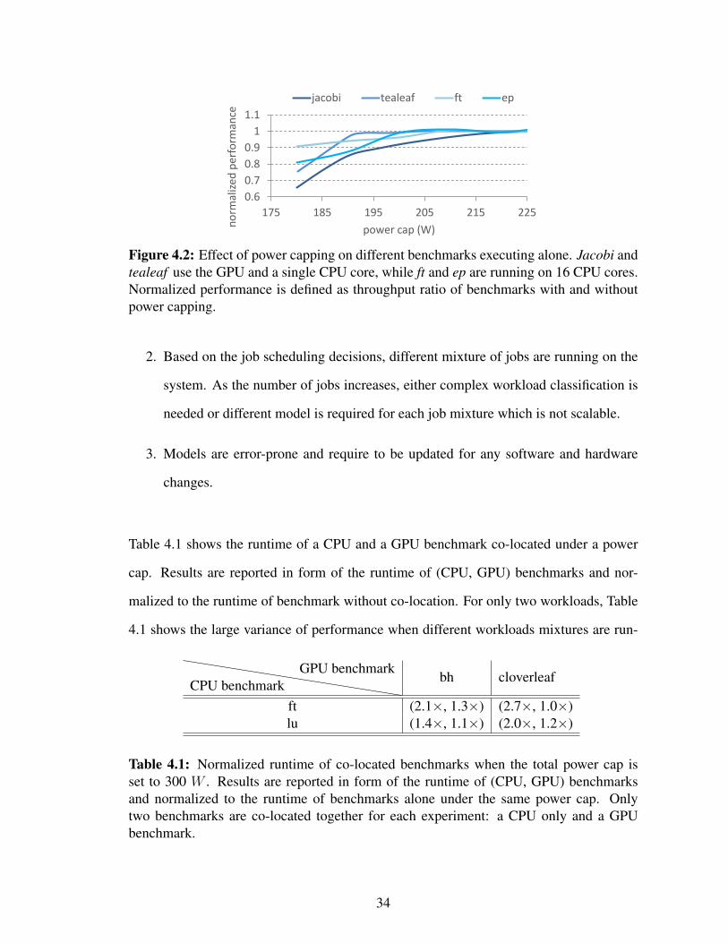
4.2 Effect of power capping on different benchmarks executing alone. Jacobiand tealeaf use the GPU and a single CPU core, while ft and ep are runningon 16 CPU cores. Normalized performance is defined as throughput ratioof benchmarks with and without power capping. . . . . . . . . . . . . . . 34

4.3 The PowerCoord framework for power capping multi-CPU/GPU servers. . 35

4.4 The details of BestChoice and how it works with other components ofPowerCoord. . . . . . . . . . . . . . . . . . . . . . . . . . . . . . . . . 45

xiii

4.5 The throughput collected for each proposed policy without BestChoicepolicy selection and POWsched [39] using different job trace and powercaps. The policies are fixed throughout the experiment. . . . . . . . . . . 54

4.6 (a) Total power cap and total power consumption of the server, and (b)power consumption of each CPU socket and GPU throughout the dynamicpower cap experiment. . . . . . . . . . . . . . . . . . . . . . . . . . . . 56

4.7 Comparing throughput for high and low priority jobs of PowerCoord withstatic policies and POWsched [39] in dynamic power cap experiment. . . 57

4.8 (a) Total number of jobs running on the server, (b) total power cap andtotal power consumption of the server, (c) power consumption of eachCPU socket and GPU throughout the dynamic job rate experiment. . . . 58

4.9 Comparing throughput for high and low priority jobs of PowerCoord withstatic policies and POWsched [39] in dynamic job rate experiment. . . . . 59

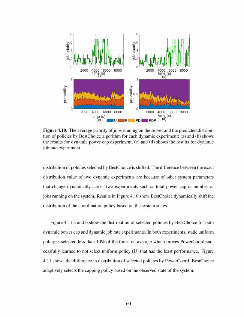
4.10 The average priority of jobs running on the server and the predicted distri-bution of policies by BestChoice algorithm for each dynamic experiment:(a) and (b) shows the results for dynamic power cap experiment, (c) and(d) shows the results for dynamic job rate experiment. . . . . . . . . . . 60

4.11 The distribution of policies selected by BestChoice algorithm at (a) dy-namic power cap experiment, (b) dynamic job rate experiment. . . . . . . 61

5.1 Structure of DPC algorithm. Jobs get submitted to SLURM and work-load monitor (WM) get the workload information from SLURM daemon(slurmd). DPC gets the workload information from WM and actuate thepower cap using the power controller (PC). . . . . . . . . . . . . . . . . . 64

5.2 The main steps of DPC algorithm. . . . . . . . . . . . . . . . . . . . . . 67

5.3 Generated graphs for DPCs agent where each vertex is a DPC agent andeach edge indicates two agents that are neighbors. Graphs are generatedfrom Watts-Strogatz model where each with β = 0 and mean degree (a)k = 4 (b) k = 8 (c) k = 12 and (d) k = 16. . . . . . . . . . . . . . . . . . 74

5.4 Detailed comparison between DPC and Dynamo for a minute of experi-ment. Panel (a): load on the web servers, Panel (b): total power consump-tion of the cluster, and Panel (c): power consumption of each sub-clusterrunning the primary (web servers) and secondary (batch jobs) workloadfor each method. . . . . . . . . . . . . . . . . . . . . . . . . . . . . . . . 83

xiv

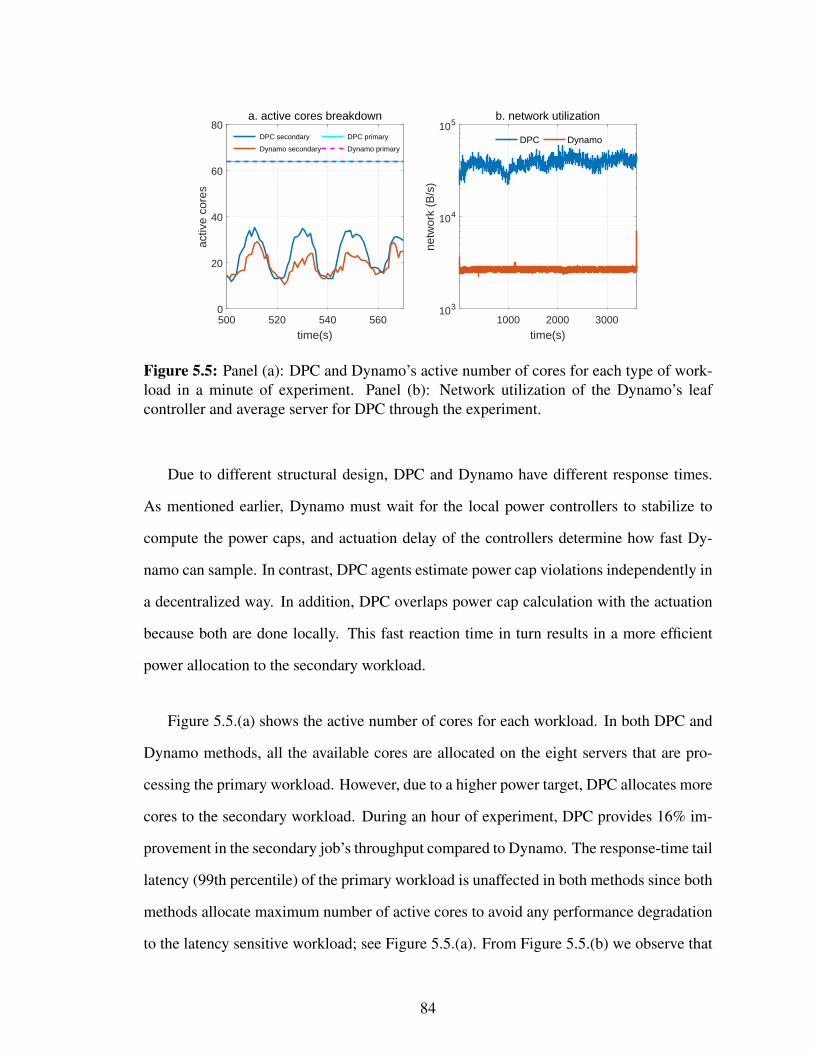
5.5 Panel (a): DPC and Dynamo’s active number of cores for each type ofworkload in a minute of experiment. Panel (b): Network utilization of theDynamo’s leaf controller and average server for DPC through the experi-ment. . . . . . . . . . . . . . . . . . . . . . . . . . . . . . . . . . . . . . 84

5.6 Modeled (lines) and observed (markers) normalized throughput as the func-tion of power consumption. . . . . . . . . . . . . . . . . . . . . . . . . . 86

5.7 Comparison between DPC, Dynamo, centralized, and a uniform powercapping under a dynamic power cap. . . . . . . . . . . . . . . . . . . . . 87

5.8 Power and number of jobs running on the cluster in the dynamic-load ex-periment. . . . . . . . . . . . . . . . . . . . . . . . . . . . . . . . . . . 88

5.9 job throughput of the two experiments. . . . . . . . . . . . . . . . . . . . 89

5.10 The power capping reaction time of each method. . . . . . . . . . . . . . 90

5.11 Total power consumption of the cluster and the average network utilizationin the case of servers failure. . . . . . . . . . . . . . . . . . . . . . . . . 92

6.1 The experimental setup overview of ScaleSoC cluster. 16 TX1 boards areconnected with both 10Gb and 1Gb switches. . . . . . . . . . . . . . . . 102

6.2 Speedup gained by using the 10GbE NIC compared to using the 1GbE fordifferent cluster sizes. . . . . . . . . . . . . . . . . . . . . . . . . . . . . 104

6.3 Normalized energy consumption when the 10GbE NIC is used comparedto using the 1GbE for different cluster sizes. . . . . . . . . . . . . . . . . 104

6.4 Normalized energy efficiency of hpl when different ratios of CPU-GPGPUwork is assigned, compared to the case where all of the load is on theGPGPU. Only one CPU core is being used per node. . . . . . . . . . . . 107

6.5 Relative runtime and events/metrics of the Cavium server compared withthe ScaleSoC cluster chosen using PLS. . . . . . . . . . . . . . . . . . . 117

6.6 Normalized runtime and L2D cache misses of the Cavium server when us-ing only one socket out of two compared to using both sockets for runningdifferent class sizes of the NPB benchmark suite. In both sets of experi-ments, the number of MPI processes is the same. The only difference is thescheduling of processes to only one and then two sockets of the Caviumserver. . . . . . . . . . . . . . . . . . . . . . . . . . . . . . . . . . . . . 118

6.7 Runtime and energy consumption of ClusterSoCBench scientific work-loads running on 8 and 16 nodes ScaleSoC cluster, normalized to two dis-crete GPGPUs. . . . . . . . . . . . . . . . . . . . . . . . . . . . . . . . 121

xv

6.8 ScaleSoC cluster throughput, memory and GPGPU utilization of Scale-SoC for Caffe and TensorFlow. Results are normalized with respect toTensorflow’s performance. . . . . . . . . . . . . . . . . . . . . . . . . . 122

6.9 Normalized throughput and unhalted CPU cycles per second of image in-ference using distributed Caffe for different scale-out cluster sizes normal-ized to the discrete GPGPUs. . . . . . . . . . . . . . . . . . . . . . . . . 123

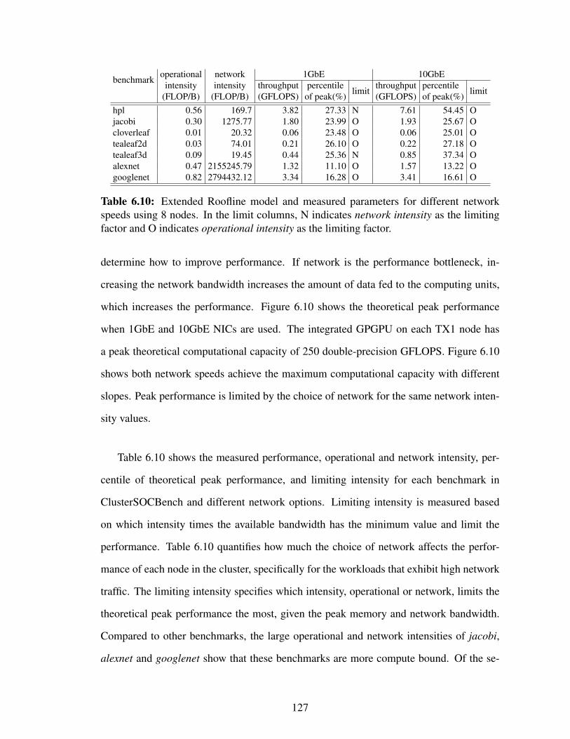
6.10 Proposed Roofline model extension for different network speeds: a) using1GbE NIC b) using 10GbE. . . . . . . . . . . . . . . . . . . . . . . . . . 126

6.11 Scalability of the benchmarks in ClusterSoCBench. Ideal network is thecase when traces are simulated assuming unlimited bandwidth betweennodes; ideal load balance is when the load is perfectly distributed amongnodes. . . . . . . . . . . . . . . . . . . . . . . . . . . . . . . . . . . . . 132

6.12 Scalability of the classical scientific workloads. . . . . . . . . . . . . . . 132

xvi

List of Tables

4.1 Normalized runtime of co-located benchmarks when the total power cap isset to 300 W . Results are reported in form of the runtime of (CPU, GPU)benchmarks and normalized to the runtime of benchmarks alone under thesame power cap. Only two benchmarks are co-located together for eachexperiment: a CPU only and a GPU benchmark. . . . . . . . . . . . . . 34

4.2 A summary of states considered for BestChoice . . . . . . . . . . . . . . 43

4.3 The pool of benchmarks considered as jobs. . . . . . . . . . . . . . . . . 49

5.1 The effect of changing topologies on DPC. . . . . . . . . . . . . . . . . . 75

5.2 The effect of update rate of DPC on the overhead. . . . . . . . . . . . . . 80

6.1 Summary of the GPGPU accelerated workloads collected in ClusterSoCBench.100

6.2 The upper bound of fast network improvement for various workloads. Re-sults are obtained by comparing the simulated execution time of workloadsunder ideal network scenario and execution time using the 10GbE network. 106

6.3 Throughput and energy efficiency using the CPU and GPGPU versions ofhpl and their collocation for different network speeds. The hybrid CPU-GPU results are estimated using 3 CPU cores for the CPU version and 1CPU core + GPGPU for the GPGPU version. . . . . . . . . . . . . . . . 108

6.4 Configuration comparison of the Cavium server and ScaleSoC cluster. . . 109

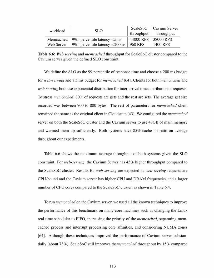
6.5 Configuration comparison of discrete GPGPU cluster with ScaleSoC clus-ter. . . . . . . . . . . . . . . . . . . . . . . . . . . . . . . . . . . . . . 111

6.6 Web serving and memcached throughput for ScaleSoC cluster comparedto the Cavium server given the defined SLO constraint. . . . . . . . . . . 113

6.7 Traditional scientific applications result for the Cavium server comparedto the ScaleSoC cluster with class size C. . . . . . . . . . . . . . . . . . . 115

xvii

6.8 Runtime, power and energy consumption of GPGPU accelerated scientificworkloads on a single TX1 node normalized to a single discrete GPGPUcard. . . . . . . . . . . . . . . . . . . . . . . . . . . . . . . . . . . . . . 119

6.9 The throughput and energy efficiency of our cluster and existing solutions.For the Cavium server, all 96 cores are used to get the results. . . . . . . . 124

6.10 Extended Roofline model and measured parameters for different networkspeeds using 8 nodes. In the limit columns, N indicates network intensityas the limiting factor and O indicates operational intensity as the limitingfactor. . . . . . . . . . . . . . . . . . . . . . . . . . . . . . . . . . . . . 127

6.11 Runtime, L2 usage, L2 throughput, and memory stalls of GPGPU run-ning Jacobi for different programming models, normalized to the host anddevice memory model. . . . . . . . . . . . . . . . . . . . . . . . . . . . 129

xviii

Chapter 1

Introduction

Computing clusters consist of large number of servers, network switches, and cooling

equipment revolutionize the computing industry. They enabled web services such as web

search, social network, and e-commerce that are being used daily by billions of people

across the planet. Computing clusters are the foundation of supercomputers that enabled

high performance computing (HPC) used in weather prediction or scientific simulations.

Cloud computing paradigm provides many opportunities by reducing the cost of compu-

tation for various industries. Total cost of ownership (TCO) for computing clusters consist

of capital and operational expenses. Capital expenses includes purchasing the equipment

and building of computing clusters while operational expenses includes the energy bill and

engineering forces to maintain the computing clusters.

Electric power is one of the scarce resources for computing clusters. Power is used

majorly for computation and extracting the heat from the facility. Large facilities are

reported to consume up to 50 MW [16, 63]. Consequently, power constrains both the

performance and profit of computing clusters. Total number of servers in a facility is

1

determined by the available power which controls the peak performance. Both capital and

operational expenses are affected by the power. The price of power delivery infrastructure,

servers and cooling equipment impacts the capital expenses, and the energy bill impacts

the operational cost. If power is managed inefficiently, more facilities must be built to

handle the high demand of computation which wastes a large amount of capital and harms

the environment.

Power is over-subscribed to increase the efficiency of power infrastructure in large fa-

cilities [18]. Power consumption of servers vary depending on their load. Cluster operators

in general use power management mechanisms to limit power consumption to safe levels

that meet the electrical specifications (e.g., circuit breaker ratings) and the cooling infras-

tructure. Cluster and node level power management systems coordinate to determine the

best power management scenario depending on the workload. Then, the node level con-

trollers actuate the decision by scaling down the power consumption of the processors,

which in turn reduces the power consumption of the whole server.

Computing clusters in general host two types of workload: 1) throughput oriented

workloads such as HPC jobs in supercomputers or batch analytical jobs in data centers,

and 2) latency sensitive workloads such as web services in data centers. Depending on the

workload, different power management scenarios must be actuated. To control the power

consumption of servers, processors makers provide multiple hardware mechanisms. Dy-

namic voltage and frequency scaling (DVFS), sleep states (C-states), and running average

power limit (RAPL) are the few technologies offered by modern processors. In this disser-

tation, we show that there exists many opportunities to increase the performance of power

constrained computing clusters. We use various hardware and software mechanisms to

improve the performance of computing clusters.

It must be mentioned nevertheless that over-subscribing power at the rack level is un-

2

safe for latency sensitive workloads, as noted by Fan. et al. [41], given that large Internet

services are capable of driving hundreds of servers to high-activity levels simultaneously.

Also, controlling the power consumption of server leads to unacceptable effect on latency

metrics. Thus, power management is done in a best-effort manner for latency sensitive

workloads. In other words, if there exists a latency slack, the performance of the server

can be reduced to save power. The saved power is used to achieve more performance for

throughput oriented workloads.

In Chapter 3, we investigate power management techniques for latency sensitive work-

loads. For modern web services, an individual application is composed of a large tree of

micro-services, each serving transactions, and similarly generating requests to other ser-

vices in the data center. Minimizing tail latency of requests is a dominant optimization

target in data centers because whole groups of requests are often held behind by the slow-

est one. In an application service tree, the negative effects of a single slow request can

easily get amplified severalfold when moving closer to the root. For example, Dean and

Barroso show a latency degradation of 10×, when measured at the root of the tree, as

opposed to at an individual node [33]. Such performance irregularities lead to violations

of service-level objectives (SLOs) and low levels of utilization in data centers [17].

Processor idleness, especially at mid- and low-utilization points, interferes with re-

quest tail latencies [53, 64]. The latency cost of sleep is the result of a request arriving

while a processor core is in a sleep state, and having to pay additional latency for the tran-

sition to active mode before being processed. Deeper sleep states lead to larger latency

transitions, which further exacerbates the problem at low server utilization. Given that

servers spend most of their time at low utilization [17], sleep states lead to a dilemma as

enabling them saves power but increases response time. We propose a sleep state arbi-

tration technique, CARB, that minimizes response time, while simultaneously realizing

the power savings that could be achieved from enabling sleep states. CARB adapts to in-

3

coming request rates and processing times and activates the smallest number of cores for

processing the current load. CARB reshapes the distribution of sleep states and minimizes

the latency cost of sleep by avoiding going into deep sleeps too often.

Next in Chapter 4, we investigate power capping for multi-CPU/GPU servers running

throughput oriented workloads. Cloud computing providers and supercomputers often

rely on server nodes that are composed of multiple sockets of CPUs and GPUs to handle

the demands of high performance intensive computations. Multi-CPU/GPU servers offer

high degree of parallelism and reduce the communication requirements over the network.

By their nature these servers consume much larger amounts of power compared to regular

commodity servers. With multiple CPU sockets, GPUs and large amount of memory, the

peak power consumption of a a single server can easily reach 500-1000 Watts depending

on its exact configuration.

We propose a new power capping controller, PowerCoord, that is specifically designed

for servers with multiple CPU and GPU sockets that are running multiple jobs at a time.

PowerCoord coordinates among the various power domains (e.g., CPU sockets and GPUs)

inside a node server to meet target power caps, while seeking to maximize throughput. Our

approach also takes into consideration job deadlines and priorities. Because performance

modeling for co-located jobs is error-prone, PowerCoord uses a learning method. Power-

Coord has a number of heuristic policies to allocate power among the various CPUs and

GPUs, and it uses reinforcement learning for policy selection during runtime. Based on

the observed state of the system, PowerCoord shifts the distribution of selected policies.

We implement our power cap controller on a real multi-CPU/GPU server with low over-

head, and we demonstrate that it is able to meet target power caps while maximizing the

throughput, and balancing other demands such as priorities and deadlines.

In Chapter 5, we investigate the power capping problem at the cluster level. A fast

4

cluster power capping method allows for a safe over-subscription of the rated power dis-

tribution devices, provides equipment protection, and enables large clusters to participate

in demand-response programs. However, current methods have a slow response time with

a large actuation latency when applied across a large number of servers as they rely on

hierarchical management systems. We propose a fast decentralized power capping (DPC)

technique that reduces the actuation latency by localizing power management at each

server. The DPC method is based on a maximum throughput optimization formulation

that takes into account the workloads priorities as well as the capacity of circuit breakers.

Therefore, DPC significantly improves the cluster performance compared to alternative

heuristics. We implement the proposed decentralized power management scheme on a

real computing cluster.

Emerging computer architectures, such as low-power ARM processors, enable a new

major direction to increase the performance of large scale clusters given their power con-

straint. Compared to the available processors in the market, ARM processors have three

main advantages: First, ARM processors are customizable by design for particular work-

load characteristics compared with the available solutions that must be purchased as gen-

eral processors found on the market. Second, ARM cores have a simpler design and much

lower power consumption compared to the available solutions. Given a fixed power bud-

get, a higher number of ARM cores can be used. Therefore, using ARM processors can

improve both performance and energy efficiency for modern workloads that have a high

degree of parallelism. Finally, ARM processors provide another source of supply which

creates competitions in the market and improves the cost efficiency of clusters.

There are two trends in available ARM SoCs in the market: mobile-class ARM SoCs

that rely on the heterogeneous integration of a mix of CPU cores, GPGPU streaming mul-

tiprocessors (SMs), and other accelerators, whereas the server-class SoCs instead rely on

integrating a larger number of CPU cores with no GPGPU support and a number of IO ac-

5

celerators. For scaling the number of processing cores, there are two different paradigms:

mobile-class SoCs use scale-out architecture in the form of a cluster of simpler systems

connected over network, whereas sever-class ARM SoCs uses the scale-up solution and

leverage symmetric multiprocessing (SMP) to pack a large number of cores on the chip.

In Chapter 6, we present ScaleSoC cluster which is a scale-out solution based on mo-

bile class ARM SoCs. ScaleSoC leverages fast network connectivity and GPGPU acceler-

ation to improve performance and energy efficiency compared to previous ARM scale-out

clusters. We consider a wide range of modern server-class parallel workloads includ-

ing latency-sensitive transactional workloads, MPI-based CPU and GPGPU accelerated

scientific applications, and emerging artificial intelligence workloads. We study the per-

formance and energy efficiency of ScaleSoC compared to server-class ARM SoCs and

discrete GPGPUs in depth for each type of server-class workload. We quantify the net-

work overhead on the performance of ScaleSoC and show that packing a large number

of ARM cores on a single chip does not necessarily guarantee better performance due to

the fact that shared resources, such as last level cache, become performance bottlenecks.

We characterize the GPGPU accelerated workloads and demonstrate that for applications

that can leverage the better CPU-GPGPU balance of ScaleSoC cluster, performance and

energy efficiency both improve compared to discrete GPGPUs. We also analyze the scal-

ability and performance limitations of the proposed ScaleSoC cluster.

6

Chapter 2

Background

In this chapter, we describe the background and related prior works that are relevant to

the proposed techniques in this dissertation. As the main goal of our proposed methods is

to improve the performance of power constrained computing clusters, we start with intro-

ducing available resources in modern processors for power management and performance

monitoring. In Section 2.2, we introduce the challenges for power capping large scale

computing clusters and summarizes the prior works. Finally, we summarize prior works

on using ARM architecture for server class computing in Section 2.3.

2.1 Processor resources for power management and per-

formance monitoring

In this section, we review the power saving and performance monitoring technologies

implemented in modern processors.

7

2.1.1 Active low power states (P-state)

Operating voltage and frequency of modern processors can be scaled down to save power

when the processors is stalled in cases such as memory stalls or last level cache stalls. We

define popular terminologies used to exploit the active low power states of processors:

Dynamic voltage and frequency scaling (DVFS)

DVFS is one the most studied power saving techniques that reduce the power consumption

of processors by dynamically selecting lower voltage-frequency operating configuration

for processors. Different feedback loops can be defined to select the operating low power

states. As an example, commodity operating systems such as Linux use the utilization to

select the operating state. When the utilization is low, lower power states are selected to

save power. When the utilization increases, higher power states are selected to increase

the performance of processor. DVFS is used widely for limiting the power consumption

of servers. The feedback loop control the active low power state to match the actual power

consumption of the server to the target power.

Running Average Power Limit (RAPL)

RAPL is the Intel’s feedback loop to control the power consumption of its processors

[32]. Users specify the maximum power the processors can consume in a time window,

then RAPL dynamically selects the operating voltage and frequency of the processor to

achieve the target power. If the load is not enough, the highest voltage and frequency is

going to be selected. Since RAPL is implemented in hardware, it is fast, accurate, and

widely used in practice.

8

2.1.2 Sleep states (C-state)

Sleep state modes enable processors to reduce their power consumption during idle time

when no instruction is available to execute. Modern processors offer many levels of sleep

states for more power savings during idle periods. As an example, the Intel’s Haswell

architecture offers the following sleep states: C1 state leads to a core halt with lower fre-

quency and voltage for the cores; C3 state leads to L1/L2 cache flush and clock shutdown;

C6 leads to saving the core’s status and voltage shut down; and C7 is similar to C6 with

an addition of L3 cache flush when all cores are idle [61].

While sleep states enable processors to achieve power savings, entry to and exit from

a C-state by a core incurs a latency overhead during which the core cannot be utilized. For

example, it is estimated that the C3 state has a latency overhead of about 80 µs, while the

C6 state has a latency overhead of about 100 µs [53].

2.1.3 Performance Monitor Unit (PMU)

Modern processors provide many performance monitoring counters (PMC) that are col-

lectable at runtime to gain information about different architectural component of proces-

sors. Various hardware events can be selected and counted with PMCs. The generally

available events include cache accesses and misses, branch prediction, memory accesses

and executed/stalled clock cycles. PMCs enable architects to characterize workloads and

identify the performance bottlenck of processors. Performance counters can be used to

predict the power consumption of processors [89, 34].

9

2.2 Power capping

To increase the efficiency of computing clusters, many servers are normally hosted by an

electric circuit than its rated power permits [18]. This power over-subscription is justified

by the fact that the nameplate ratings on servers are higher than the servers’ actual power

utilization. Moreover, rarely all servers work at their peak powers simultaneously. In the

case that the power consumption of subscribed servers peak at the same time and exceed

the circuit capacity, power must be capped quickly to avoid tripping the circuit breakers.

Also, power capping can be used as a safety measure to reduce power consumption of

servers when supporting equipment fails. For instance, the breakdown of a data center’s

computer room air conditioning (CRAC) system may result in a sudden temperature in-

crease of IT devices [12]. In this scenario, power capping can help maintain the baseline

temperature inside a facilty. Dynamic power capping regulates the total power consump-

tion under dynamic time-varying power caps. This is an important feature for short-term

trading where energy transactions are cleared simultaneously to match electricity supply

with demand in real time [25]. Even in a more static day-ahead energy market, fluctua-

tions in diurnal pattern of submitted queries may necessitate a fast response from power

management tools to ensure an optimized performance for the cluster.

Power capping problems must be solved at the cluster and node levels. Figure 2.1

shows the overview of power capping implementation for computing clusters. Cluster

level controller decides the power capping scenario based on the running workload on

each server and coordinate the decision between nodes to maximize the performance of

the cluster. Node level controllers get the decision from the cluster level controller and

select the best configuration for the server to maximize its performance.

At the cluster level, an important issue in power capping techniques is to select an

10

power & workload info

power target

each server actuates locally

cluster levelcontroller

node levelcontroller

serv

er &

w

orkl

oad

info

conf

igur

atio

n



Figure 2.1: The overview of power capping implementation at the cluster and node level.

appropriate power cap in order to maximize the number of hosted servers in a data cen-

ter [45]. A common practice is to ensure that the peak power never exceeds the branch

circuits capacity as it causes tripping in circuit breaker (CB). However, this approach is

overly conservative. The power cap for each server must be selected in a way to maximize

the cluster’s performance and meet the circuit breakers capacity. By carefully analyzing

the tripping characteristics of a typical CB, the system’s performance can be optimized

aggressively through power over-subscription without the risk of tripping CB.

At the node level, many hardware and software mechanisms can be used to control

the power. Power saving states for processors are the example of hardware mechanisms.

Workload consolidation to a subset of cores can be used to control the power as a software

technique. The node level controller, must select the best software/hardware configuration

to meet the power target selected by the cluster level controller while trying to maximize

the performance of the node.

11

2.2.1 Cluster level power capping

The main challenge in implementing coordinated power capping is to limit the actuation

latency of controllers. A detailed examination of latency in hierarchical models [18] shows

that even a small actuation latency, i.e., the latency in control knobs, can cause instability

in hierarchical, feedback-loop power capping models. The main difficulty is due to the fact

that when feedback loops operate on multiple layers in the hierarchy, stability conditions

demand that the lower layer control loop must converge before an upper layer loop can

begin the next iteration. Despite this observation, recently a hierarchical structure for

power capping, dubbed as Dynamo, has been proposed and implemented on Facebook’s

data center [97].

Dynamo uses the same hierarchy as the power distribution network, where the lowest

level of controllers, called leaf controllers, are associated with a group of servers. In this

framework, priorities of workloads are determined based on the performance degradation

that they incur under power capping. Power consumption of the lowest priority workloads

are ranked in buckets and power is reduced based on a high-bucket-first approach, where

the algorithm uniformly reduces the total-power-cut from the nodes that are consuming

the most power. If power is needed to be reduced further, Dynamo moves to the next

buckets and workload priorities.

2.2.2 Node level power capping

Power capping has been extensively studied for CPU workload at the node level [28, 67,

101, 88]. Cochran et al. proposed Pack & Cap which used thread packing and adjusting

the DVFS to cap the power [28]. Liu et al. proposed FastCap which scales well for

12

large number of CPU cores [67]. FastCap is based on a non-linear optimization approach

which considered both CPU and main memory DVFS. Zhang et al. proposed PUPiL as

a hybrid approach for CPU power capping [101]. PUPiL uses RAPL to limit the power

consumption fast, while searching the best configuration to maximize the performance

given the power limit.

While many works looked at power capping for CPUs, a few works considered GPGPU.

Komoda et al. considered power capping by coordinating the DVFS and task mapping be-

tween CPU and GPU [57]. Their method is only applicable if the workload uses both

CPU and GPU for computation. As the workload complexity increases, GPUs are used to

do the heavy computation and CPU cores are used for data movements and synchroniza-

tion. Tsuzuku et al. considered a single workload running on the server and solved power

capping using performance modeling [92]. Ellsworth et al. proposed POWsched which

dynamically caps the power of servers with multiple power domains [40, 39].

2.3 Low-power processors for server computing

ARM 64-bit processing has generated enthusiasm to develop ARM-based servers that are

targeted for both data centers and supercomputers. In addition to the server-class com-

ponents and hardware advancements, the ARM software environment has grown substan-

tially over the past decade. Major development ecosystems and libraries have been ported

and optimized to run on ARM environment, making ARM suitable for server-class work-

loads.

Examining existing and planned server-based ARM System-on-a-Chip (SoC) proces-

sors shows that upcoming server-class SoCs are trending toward a scale-up solution that

13

uses Symmetric Multi-Processing (SMP) to include a large number of CPU cores on the

chip. For instance, Applied Micro’s X-Gene 1 contains 8 ARM cores, the planned X-Gene

3 will have 32 cores, and Cavium’s ThunderX SoC packs 48 ARMv8 cores per socket. In

addition to CPU cores, these SoCs include IP blocks for a memory controller and high-end

network and I/O connectivity.

The makeup of server class SoCs is different from mobile-class ARM SoCs that em-

phasize heterogeneous integration of fewer CPU cores at the expense of Graphical Pro-

cessing Unit (GPU) Streaming Multiprocessors (SMs). While these GPU cores have his-

torically been dedicated solely to graphics, modern mobile-class ARM SoCs incorporate

general-purpose GPUs (GPGPU) that can be programmed to accelerate workloads. Com-

pared to the discrete GPGPUs, the integrated GPGPUs have lower specs namely slower

clock speeds and fewer SMs. For comparable core counts with scale-up solutions, these

low-end mobile-class ARM SoCs must use a scale-out architecture in the form of a cluster

connected over a network.

A number of studies recently appeared that focus on the use of low-power, mobile-

class ARM SoCs in the HPC domain [60, 82, 85, 84, 83]. Rajovic et al. designed a

HPC cluster, Tibidado, with 128 nodes, where each node is based on a mobile 32-bit

Nvidia Tegra2 SoC featuring dual Cortex-A9 cores [82, 85, 84]. The study points to a

number of limitations (e.g. lack of ECC protection and high network bandwidth) that

arise from using mobile platforms. Mont-Blanc is the latest prototype that uses mobile-

class ARM SoCs [83]. Mont-Blanc is based on Cortex A15 (ARMV7) and uses 1GbE

for network communication. Unlike with Tibidabo, where its integrated GPUs were not

programmable, the integrated GPGPUs used in the Mont-Blanc cluster are programmable

using OpenCL. However, the Mont-Blanc study only evaluates the CPU performance of

the cluster.

14

For server-class ARM SoCs, a recent study compares the performance and power of

the X-Gene 1 SoC against the standard Intel Xeon and the recent Intel Phi [8]. The result

concludes that these systems present different trade-offs that do not dominate each other,

and that the X-Gene 1 provides a higher energy efficiency, measured in performance/watt.

Azimi et al. evaluated the performance and energy efficiency of X-Gene 1 SoC and x86

Atom for scale-out and high-performance computing benchmarks [13]. They discussed

the impact of the SoC architecture, memory hierarchy, and system design on the perfor-

mance and energy efficiency outcomes.

Latency sensitive workloads typically have lower communication needs between its

threads, which enables them to scale gracefully on parallel clusters. Ou et al. analyze the

energy efficiency of three latency sensitive applications (web server, in-memory database

and video transcoding) and concluded that the ARM cluster is between 1.2 and 9.5 times

more energy efficient than an x86 workstation that uses an Intel Core-Q9400 processor

[79]. For I/O-dominated workloads, the FAWN cluster couples lightweight Atom x86

processors in a well-balanced system with a solid-state HDD and 100 Mbps Ethernet [9].

Compared to traditional disk-based clusters, FAWN achieves two orders of magnitude of

improvements in queries per Joule. Attempts to replicate the same success with complex

database workloads have led to poor results compared to traditional high-end x86 servers

[62].

As for the x86 versus ARM debate, [19, 11, 50], Blem et al. compare 32/64-bit x86

against 32-bit ARMv7 SoC-based platforms using several workloads that are represen-

tative of mobile, desktop and server domains [19]. The analysis mostly focuses on the

SPEC CPU06 benchmarks, with additional results from two server applications (a web

search and a web server). By analyzing the number of instructions and instruction mix

and their impact on performance and power, the comparison concludes that instruction set

architecture (ISA) effects are indistinguishable, that it is the better branch predictor and

15

larger caches that give x86 processors a lead in performance over ARM processors. The

study also concludes that the ARM and x86 systems are engineered for different runtime

and power consumption trade-offs. Jundt et al. compared the x86 versus XGene 1 and

used hardware performance counters to find the bottleneck of performance [52].

16

Chapter 3

Power management for latency sensitive

workloads

In this chapter, we propose a c-state arbitration technique, CARB, that minimizes response

time, while simultaneously realizing the power savings that can be achieved from enabling

sleep states. In Section 3.1, we motivate our approach. Section 3.2 gives the details of our

methodology and in Section 3.3 we evaluate the performance of CARB on a real server in

dynamic scenarios. We finish this chapter, by summarizing our findings in Section 3.4.

3.1 Motivation

The rise of online services in the last decade has led to a computation model in which “the

data center is the computer [16].” In this model, an individual application is composed of

a large tree of micro-services, each serving transactions, and similarly generating requests

to other services in the data center. The data centers that carry these large-scale Internet

17

applications are a distinctively new class of machines that adopt different metrics from tra-

ditional shared hosting environments. Designing and programming data centers requires

a careful balance between consistent and predictable high performance on the one hand,

and cost- and energy-efficiency on the other.

On the performance side, tail request latency is a dominant optimization target, since

whole groups of requests are often held behind by the slowest one. In a application service

tree, the negative effects of a single slow request can easily get amplified severalfold when

moving closer to the root. Such performance irregularities can easily lead to violations of

service-level agreements (SLOs) at scale, and are one of the primary reasons for habitually

low levels of utilization in data centers [17].

Energy-wise, data centers have been the target of a significant body of research [16,

20, 68]. For data center capacity planning and power provisioning purposes, it is desirable

that servers are energy-proportional [16, 41]; that is, that they scale power consumption

with utilization. Processor idle modes, which clock- and power-gate different portions of

a chip, are crucial for achieving the current levels of proportionality [36, 53, 74].

Power savings states, i.e., c-states, enable processors to save power consumption dur-

ing idle periods where no instructions are available to execute. New processors offer

deeper sleep states for more power savings during idle periods. For example, Intel’s

Haswell architecture offers the following 5 c-states (e.g., C1, C1E, C3, C6 and C8) [61].

While c-states enable processors to achieve power savings, entry to and exit from a c-state

by a core incurs a latency overhead during which the core cannot be utilized. For example,

it is estimated that the C3 and C6 states require, respectively, 80 µs and 104 µs [53]. These

entry-exit latencies can have significant performance effects on workloads whose request

processing latencies are of similar magnitude.

18

0

0.05

0.1

0.15

0.2

0.25

0.3

10 20 30 40 50 60 70 80 90 100 95th percen4

le latency (m

s)

requests per second (in thousand)

c-‐state disabled c-‐state default

50

60

70

80

90

100

110

10 20 30 40 50 60 70 80 90 100

power (W

aF)


Figure 3.1: Impact of enabling versus disabling c-states on 95-th percentile latency andpower consumption for various RPS.

We illustrate the negative performance effects of deep sleep states on our 8-core Haswell-

based Xeon server in Figure 3.1. We report the 95th percentile response time and average

power consumption for the memcached application as a function of the number of re-

quests per second (RPS). The plots show that enabling c-states introduces a latency over-

head that is a function of RPS, but it reduces power consumption. For instance, at low

RPS values (e.g., 10K), the increase in the 95th response time is up to 2×, but the power

savings are about 20%. As RPS increases, there are naturally fewer opportunities for cores

to go idle, and as a result the overhead of c-states diminishes.

Figure 3.2 provides the fraction of time spent by the entire processor (averaged over 8

cores) in various c-states. The plot shows that at low RPS values, idleness periods are long

enough to induce deep sleep states with larger delay penalties. One way to mitigate this

increase in latency is to use fewer cores. We observe the relationship between the number

of active cores and latencies for memcached in Figure 3.3, where we plot the measured

95th response time as a function of the number of active cores at RPS=25K, 50K, and

75K.

The plot for each RPS value has a clear minimum where performance is optimal. To

19

0% 10% 20% 30% 40% 50% 60% 70% 80% 90%

100%

10 20 30 40 50 60 70 80 90 100 110 120 frac1o

n of c-‐state re

siden

cy


C6 C3 C1 C0

Figure 3.2: Fraction of time spent by the entire processor at various c-states.

0 0.05 0.1 0.15 0.2 0.25 0.3 0.35 0.4

1 2 3 4 5 6 7 8

95th percen4

le latency (m

s)

number of cores

rps = 25K rps = 50K rps = 75K

Figure 3.3: 95th percentile response time as a function of number of arbitrated activecores for RPS=25K, 50K and 75K.

the left of the minimum, the number of active cores is not sufficient to handle the load,

and latency dramatically increases due to queueing. More interestingly, to the right of the

minimum, performance is also worse due to the c-state latency effect identified earlier. At

the optimal point, the entry-exit overheads are minimal because the busy cores have the

minimum amount of idle time that allows them to handle the incoming load.

Based on these observations, we propose a c-state arbiter which arbitrates the number

of active cores in search for this optimum. Such behavior is in contrast with traditional

OS fairness policies, which aim to spread load across all cores, and closer to the goals

20

of packing schedulers [42]. Packing cores, or limiting an application’s core allocation,

has been well-studied, most frequently in a multi-application scenario with the goal of

workload isolation [69], i.e. not falling off the “performance cliff” shown to the left on

Figure 3.3. On the contrary, our results demonstrates that too many cores can also be

detrimental to performance even in the single-application case. While previously such

effects have been attributed to cache sharing [91] or I/O interrupt scheduling [64], we

add deep sleep as a reason to prefer packing. C-state management is highly relevant to

applications that are latency-sensitive and that lead to frequent sleeps, where the sleep

overhead is comparable to the request latency [53].

3.2 Methodology

Latency sensitive workloads in data centers have tight response time requirements to meet

service-level objectives (SLOs). Sleep states (c-states) enable servers to reduce their power

consumption during idle times; however entering and exiting c-states is not instantaneous,

leading to increased transaction latency. We observe that there is an optimal number of

active cores that minimizes tail latencies, and that any larger number of active cores be-

yond the optimal simultaneously worsens performance and power. This optimal number

is a function of the request rate and the application. Based on this observation, we propose

a c-state arbitration technique, CARB, which unobtrusively monitors request latencies for

the target workload and optimally adjusts the number of active cores to minimize response

time and power. CARB reshapes the distribution of c-states and minimizes the latency cost

of sleep by avoiding going into deep sleeps too often.

CARB is a feedback-based controller that arbitrates the minimum number of sufficient

cores for a given request rate. CARB collects the real time request rate r(k) and response

21

Algorithm 1: Control logic at S0if r(k) > r(k − 1) + δr thenc(k)← c(k − 1) + ∆(k); s(k + 1)← S1

else if r(k) < r(k − 1)− δr thenc(k)← c(k − 1)−∆(k); s(k + 1)← S2

else if y(k) > y(k − 1) + δy thenc(k)← c(k − 1) + ∆(k); s(k + 1)← S1

elsec(k)← c(k − 1) ; s(k + 1)← S0

end if

Algorithm 2: Control logic at S11: if y(k) < y(k − 1) + δy then2: c(k)← c(k − 1) + ∆(k); s(k + 1)← S13: else4: c(k)← c(k − 1)−∆(k); s(k + 1)← S05: end if

Algorithm 3: Control logic at S21: if y(k) < y(k − 1) + δy then2: c(k)← c(k − 1)−∆(k); s(k + 1)← S23: else4: c(k)← c(k − 1) + ∆(k); s(k + 1)← S05: end if

time y(k) (time is discrete and denoted by k) as control inputs and arbitrates the number

of active cores.

At each control epoch, CARB adjusts the number of active cores c(k) ∈ [cmin, cmax]

towards the optimal. CARB has three working states: 1) idle state S0, where it measures

the request rate r(k) and the response time y(k) and determines the next state s(k+ 1); 2)

scaling up state S1, where it increases the number of active cores by a step size ∆(k) until

the response time cannot be further improved, then switches back to S0; and 3) scaling

down state S2, where it decreases the number of active cores by ∆(k) until the response

time cannot be further improved, then switches back to S0. In more detail, when the

controller resides in S0, the state transitions and control logic are given in Algorithm 1. δr

22

and δy are sensitivity thresholds to filter out the noise in request rate and response time so

that unnecessary oscillation can be avoided, and are determined empirically.

At states S1 and S2, CARB scales the number of active cores (up for S1 and down for

S2) towards the optimal as given in Algorithms 2 and 3. At initialization, we set k = 0,

c(0) = cmax, and s(0) = S2 while measuring r(0) and y(0). In all steps, CARB checks

that ∆(k) leads to a c(k) ∈ [cmin, cmax] before each change inside the loop. It is crucial

to identify the most effective step size ∆(k), particularly when CARB is operating on the

left side to the optimal on the curve in Figure 3.3. To ensure the SLO will not be violated,

CARB should move out of the left side within the minimum number of steps. A constant

∆(k) can be set based on user preferences and might be chosen differently for scaling

up and scaling down. To address the situation of potential bursts in request load, which

requires scaling up capacity rapidly, CARB sets the number of cores to the maximum

when the request rate r(k) increases beyond a threshold rth, then attempts to scale down

cores afterwards.

We also examined other controllers based on proportional-integral-derivative (PID)

controllers and gradient descent methods. PID controllers require analytical models for

the output to identify their optimal parameters, which is quite challenging in our system

due to the variations in the response time from queuing effects. On the other hand, CARB

does not require an analytical objective function. Similarly, optimal control methods (e.g.,

gradient descent or Newton’s method) require a differentiable objective function. We have

found that noise arising from measurements and queuing effects lead to erroneous gradient

calculations, which make these methods relatively unstable. As our problem is a local one-

dimensional unconstrained optimization problem, our bang-bang based CARB controller

gives us good results.

23

3.3 Evaluation

3.3.1 Experimental Setup

Server

We evaluate CARB on an Intel Haswell-based server using a Xeon E5-2630 V3 8-core

processor with 32GB of DDR4 memory and a 10 Gbe network controller. The server

runs Ubuntu 14.04. We measure power consumption by sensing the external current at the

120 V AC socket with a sampling rate of 10 Hz. Hardware control of frequency (Intel

TurboBoost) is enabled on the processor.

Workloads

To evaluate the effectiveness of CARB, we choose memcached [44], a memory object

caching workload. The data caching benchmark from CloudSuite [43] is used to

generate request load and to collect end-to-end delay statistics.

Request load trace

Since real load traces of a data caching cluster are rarely available for access, we use a

synthetic trace. This way, we can control the range and the frequency of the fluctuation of

the requests. A time series trace can be generated using: r(k+ 1) =∑m−1

i=0 ω(i)r(k− i) +

Φα(k), where r(k) is the request load at time k, ω is a vector defining the weights on the

last m samples; Φ is a parameter that describes how much the request load will fluctuate

24

between two consecutive elements in the series; and α(k) is a random number drawn from

a normal distribution.

Implementation

CARB is implemented using Python. The number of active cores can be changed either

by setting core affinity (cpuset), or by taking cores away from the OS. In either case,

inactive cores go the deepest sleep state and the application needs no changes. CARB only

needs the ability to monitor request rate and response time of the application. The request

rate can be measured from the network socket and the response time can be observed from

the server by timing the request service time. Both of them can be measured without

modifying the target application. Although in our case data caching has the interface

to monitor the request rate and response time.

3.3.2 Experimental Results

Static results

We first demonstrate the optimal number of cores and the response time difference be-

tween using all cores and the optimal number of cores. We vary the request rate from 10

K to 120 K with a step of 10 K and measure the 95th percentile of the response time when

all 8 cores are enabled and when the optimal number of cores are enabled using CARB.

Results normalized to the response time of 8 cores, together with the corresponding num-

ber of optimal cores, are given in Figure 3.4. By consolidating the requests onto a subset

of cores, response time can be reduced by up to 51%. In order to better demonstrate how

CARB works, Figure 3.5 plots the change in c-states distribution when the request rate is

25

1

2

3

4

5

6

7

8

0

0.2

0.4

0.6

0.8

1

1.2

10 20 30 40 50 60 70 80 90 100 110 120 op/m

al num

ber o

f cores

norm

alize

d latency

K request per second

normalized latency

op/mal # of cores

Figure 3.4: The normalized 95th latency with the optimal number of cores.

0 1 2 3 4 5 6 7core id

0%

20%

40%

60%

80%

100%

fra

ction o

f c-s

tate

s r

esid

ency (a) c-states default

0 1 2 3 4 5 6 7core id

0%

20%

40%

60%

80%

100%(b) optimal arbitation

C0C1C2C6

Figure 3.5: Fraction of time spent by each core in various c-states under various arbitra-tion for RPS=10K. Subfigure (a) gives the default case when all cores are active; Subfigure(b) gives the case when 2 active cores are arbitrated.

10 K, using 8 cores and optimal number of cores (two in this case). The optimal number of

active cores is usually less than eight when the request rate is less than 100 K. We observe

that the optimal number of cores has to be larger than one, i.e., cmin = 2. One explana-

tion for this is that, with only one core available, all system and background processes

are scheduled together and interfere with the memcached process. Thus, in our dynamic

experiments, we set the lower bound of scaling down cores as two cores.

26

0 10 20 30 40 50 60 70 80 900

5

x 104

rps

0 10 20 30 40 50 60 70 80 900

0.1

0.2

95th

late

ncy(m

s)

0 10 20 30 40 50 60 70 80 9050

100

pow

er

(Watt)

0 10 20 30 40 50 60 70 80 900

5

10

# o

f active c

ore

s

time (min)

CARB c−state default c−state disabled

Figure 3.6: Dynamic results of memcached with slow varying request trace.

0 10 20 30 40 50 60 70 80 900

5

x 104

rps

0 10 20 30 40 50 60 70 80 900

0.1

0.2

95th

late

ncy(m

s)

0 10 20 30 40 50 60 70 80 9050

100

pow

er

(Watt)

0 10 20 30 40 50 60 70 80 900

5

10

# o

f active c

ore

s

time (min)

CARB c−state default c−state disabled

Figure 3.7: Dynamic results of memcached with fast varying request trace.

27

115%

79%

116%

80%

156%

84%

154%

84% 100% 100% 100% 100%

0.0

0.5

1.0

1.5

2.0

95th latency (slow varying)

power (slow varying)

95th latency (fast varying)

power (fast varying)

norm

alize

d summary

CARB c-‐state default c-‐state disabled

Figure 3.8: Summary of dynamic experiments of memcached.

Dynamic results

In this experiment we evaluate CARB with 90-minute synthetic request traces. We set the

step size ∆(k) to 1 for both scaling up and scaling down states. The threshold parameter,

rth, is chosen as 20 KRPS. The sensitivity parameter δr is set as 5 KRPS and δy is chosen

as 10% of the average response time. Figure 3.6 shows results with a slow varying trace,

where we plot the request rate, the 95th percentile of the response time, power, and the

number of active cores over time for three cases: (1) default c-state management, (2)

disabling c-states, and (3) CARB. The response time using CARB is almost half that of

the default c-state management when the request load is very low and overall 26% lower,

while consuming 6.1% less power. Compared to disabling c-states, CARB reduces power

by 23% while offering similar response times. The results are summarized in Figure 3.8.

Thus, CARB delivers response times close to the case with c-states disabled and consumes

less power than the default c-state governor.

We repeat the same test with a fast varying request rate trace. The corresponding

results are given in Figure 3.7 and Figure 3.8. The results show that the response time of

28

CARB closely follows the case with disabled c-states when request load is low. After the

load spikes at 28 mins and 57 mins, to be conservative, CARB scales up to the maximum

number of cores and then searches down for the optimal. Overall, CARB reduces response

time by 25% over the c-state default with 5% power savings.

3.4 Summary

For latency sensitive workloads with sub-millisecond response times, c-state transitions

constitute a good portion of overall latency, especially when the request load is relatively

low. In this case, consolidating the load on a subset of cores improves both latency and

energy efficiency. We devised a controller, CARB, which arbitrates the core allocation of

memcached, and manages to find the minimum number of cores to optimize latency and

power. In addition to memcached, we believe that CARB is particularly attractive for

latency-sensitive workloads, where the overhead of sleep state transitions is comparable

to the response time. Overall, CARB reduces the response time by 25% compared with

the default c-states while saving 5% more power.

29

Chapter 4

Coordinated Power Capping for

Multi-CPU/GPU Servers

In this chapter, we propose a new power capping controller, PowerCoord, that is specifi-

cally designed for servers with multiple CPU and GPU sockets that are running multiple

jobs at a time. We observe that multi-CPU/GPU servers create three unique challenges

for power capping controllers. First, these servers have multiple CPU sockets and GPUs,

each with its own power domain controller (e.g., RAPL), and as a result, meeting a given

power cap must involve coordination among the various domain controllers on the same

server. Second, workload characteristics often shift among the CPUs and the GPU, which

requires the controller to shift power budgets between the CPU(s) and the GPU(s), while

still maintaining the cap. Third, multi-CPU/GPU servers often host multiple jobs to fully

utilize their resources; these jobs have various priorities and deadline requirements that

have to be taken into consideration during capping to mitigate the impact of capping on

performance. Based on our observations, we propose a new coordinated power capping

technique that is specifically devised for server nodes with multiple CPU and GPUs. The

30

big challenge we address is to dynamically find the share of each power domain (CPU

socket, GPU) from the fixed power budget to maximize the throughput of the server that

is running multiple-jobs with various requirements. The contributions of this chapter are

as follows.

• Our power cap controller, PowerCoord, dynamically coordinates among the power

budgets of various domain controllers in a multi-CPU/GPU server to meet target

power caps, while by shifting power seeks to maximize the performance within the

power cap. Our PowerCoord controller also takes into account running a mixture of

jobs with various priorities and deadlines.

• We propose multiple heuristic policies that work for different scenarios of workload

characteristics. These policies coordinate and shift power among the different power

domains (e.g., CPU sockets and GPU), while trying to maximizing the performance

of node.

• Because each proposed policy work for different workload characteristic, we pro-

pose BestChoice algorithm that uses reinforcement learning’s actor-critic method-

ology to choose among policies in an online fashion. Based on the observed state

of the system, BestChoice learn to shift the distribution of selecting policies and

automates the process of matching workload characteristics to policy selection.

BestChoice continuously updates itself with the performance feedback of the sys-

tem.

• Our work is also the first to consider a learning method for power coordination in

multi-CPU/GPU servers. Prior works on power capping for multi-domain servers

used heuristics methods or were running a single job at a time.

• We fully implement our power capping controller on a server with two Xeon CPU

sockets (a total of 28 cores), a Nvidia P40 GPU card and 128 GB of DDR4 DRAM.

31

Our controller shows effective operation with negligible overhead across a wide

range of workload and power capping scenarios.

The organization of the rest of this chapter is as follows. In Section 4.1, we use real

workload and power traces from a multi-CPU/GPU server to motivate our work. In the

methodology section 4.2, we describe the main components of our PowerCoord controller,

which includes a number of power capping policies, a policy selection mechanism to

choose among policies during runtime, and a binder to track jobs on various sockets.

In Section 4.3 we provide a comprehensive experimental evaluation of our technique. Fi-

nally, we summarize the main conclusions of our work in Section 4.4.

4.1 Motivation

Servers with multiple CPU sockets and multiple GPU cards run a mixture of jobs to in-

crease their resource efficiency [26, 95, 69, 54]. A typical job can rarely use all the avail-

able resources of a modern server. Figure 4.1.a shows the power consumption of our

server with two CPU sockets and a discrete GPU when a mixture of jobs are running on

the node over time and no power capping is enforced. Jobs are submitted at different times

and resources can get idle at some points in time. Figure 4.1.b shows the breakdown of

power consumption between each CPU socket and GPU. The figure shows each domain

(e.g., CPU socket and GPU) has dynamic power consumption depending on the resource

utilization and characteristics of running jobs.

When the total power needs to be capped, power consumption of each CPU and GPU

needs to be reduced. In practice, each power domain (e.g., CPU sockets and GPU) has a

power controller to actuate a target budget. However, the challenge is to coordinate the

32

0 50 100 150 200 250 300time (s)

200

300

400

500

600

pow

er (

W)

(a)

total power consumption

0 50 100 150 200 250 300time (s)

50

100

150

200po

wer

(W

)

(b)

socket 1 socket 2 GPU

Figure 4.1: (a) Total power consumption of a multi-CPU/GPU server when running amixture of jobs over time, and (b) power consumption of each socket and the GPU. Nopower capping is enforced.

power budget of all domains to maximize the performance of the node and meet the perfor-

mance requirement of various jobs. To maximize the performance, the power budget must

be shifted dynamically from idle domains to the active domains that require more power.

When all domains are busy and power needs to be capped, power must be divided based on

the scheduled jobs on each domain. Depending on the resource usage and characteristic of

running jobs, power capping affects the performance of various workload differently. Fig-

ure 4.2 shows the normalized throughput of various CPU and GPU benchmarks running

on our system alone for different caps.

A workload performance could be modeled as a function of power cap when a single

benchmark is running on the system [92, 22]; however, when multiple jobs are co-located

on the system, modeling the performance is not practical for three reasons:

1. Complex resource contention makes the models complicated. Complicated models

are not beneficial for power capping solutions based on an optimization problem or

control-theoretic approaches.

33

0.6

0.7

0.8

0.9

1

1.1

175 185 195 205 215 225

no

rmal

ized

per

form

ance

power cap (W)

jacobi tealeaf ft ep

Figure 4.2: Effect of power capping on different benchmarks executing alone. Jacobi andtealeaf use the GPU and a single CPU core, while ft and ep are running on 16 CPU cores.Normalized performance is defined as throughput ratio of benchmarks with and withoutpower capping.

2. Based on the job scheduling decisions, different mixture of jobs are running on the

system. As the number of jobs increases, either complex workload classification is

needed or different model is required for each job mixture which is not scalable.

3. Models are error-prone and require to be updated for any software and hardware

changes.

Table 4.1 shows the runtime of a CPU and a GPU benchmark co-located under a power

cap. Results are reported in form of the runtime of (CPU, GPU) benchmarks and nor-

malized to the runtime of benchmark without co-location. For only two workloads, Table

4.1 shows the large variance of performance when different workloads mixtures are run-

CPU benchmarkGPU benchmark

bh cloverleaf

ft (2.1×, 1.3×) (2.7×, 1.0×)lu (1.4×, 1.1×) (2.0×, 1.2×)

Table 4.1: Normalized runtime of co-located benchmarks when the total power cap isset to 300 W . Results are reported in form of the runtime of (CPU, GPU) benchmarksand normalized to the runtime of benchmarks alone under the same power cap. Onlytwo benchmarks are co-located together for each experiment: a CPU only and a GPUbenchmark.

34

job scheduler

users

job, deadline (𝑑𝑖), priority (𝑝𝑟𝑖)

cluster level power

controller

jobs info

power consumption (P, 𝑝𝑗)

total power cap (𝐶)

…

power budgets (𝑏𝑗)

domain controller

domain controller

domain controller

domain controller

PowerCoord controller

Binder BestChoice Policies

Figure 4.3: The PowerCoord framework for power capping multi-CPU/GPU servers.

ning. As optimization and control theoretic methods require modeling the performance,

PowerCoord is motivated to use a learning-based method.

4.2 Methodology

The main structure of our power capping framework is shown in Figure 4.3. Users submit

jobs to the job scheduler to execute. We assume each job has a priority and a deadline. We

used SLURM as scheduler, and by default SLURM terminates jobs that pass their deadline

[99]. In multi-CPU/GPU servers, each CPU socket and GPU is a power domain that has

its independent power controller to monitor and actuate a target budget. Our controller,

PowerCoord, receives the total power cap from the cluster power coordinator, running jobs

information, power consumption of the server, and power consumption of each domain.

It then determines the budget for each power domain to cap the total power at the given

total cap, while seeking to maximize the server throughput. The controller of each power

domain receives its budget from PowerCoord and actuates it.

35

PowerCoord focuses on intra-node power capping which gets the server’s power cap

as input from cluster-level power capping such as Dynamo [97] that is responsible to

coordinate power between different nodes. Both capping and scheduling decisions are

hierarchical decisions, we get the cluster level decisions as inputs and focus on the node-

level optimization.

In this section, we first formulate our power capping problem. Next, we explain each

component of PowerCoord in details. Power capping is formulated as a constrained max-

imization problem. The goal is to maximize the performance subject to the power con-

straints. More specifically, we assume a set of n running Jobs = {job1, · · · , jobn} over

a period of time. Let fi, di, and pri be the finish time, deadline, and priority of jobi re-

spectively. The deadline is defined based on the runtime of the job and not the queuing

time to get scheduled. At any time, multiple jobs could be running on the server with a

set of power domains H . We assume a server has m CPU sockets and k GPUs. In our

framework, we only consider CPU sockets and GPUs as power domains and cap the total

power of the server; however, the same methodology is applicable if the power of other

components such as DRAM are controllable in future servers.

H , {CPU1, · · · , CPUm, GPU1, · · · , GPUk}.

Let pj and bj be the power consumption and budget of power domain j ∈ H re-

spectively. Each power domain has an independent controller that actuates the budget

(pj ≤ bj). Let pminj and pmax

j be the minimum and maximum power consumption of power

domain j ∈ H respectively. C and P denote the total power cap and total power con-

sumption of the server. Total power consumption of the server is the sum of its power

domains plus the power consumption of other components such as DRAM, motherboard,

36

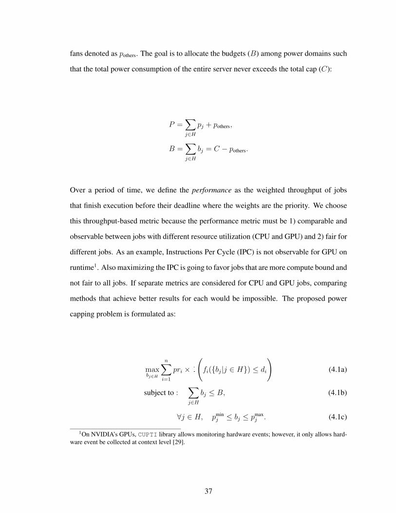
fans denoted as pothers. The goal is to allocate the budgets (B) among power domains such

that the total power consumption of the entire server never exceeds the total cap (C):

P =∑j∈H

pj + pothers,

B =∑j∈H

bj = C − pothers.

Over a period of time, we define the performance as the weighted throughput of jobs

that finish execution before their deadline where the weights are the priority. We choose

this throughput-based metric because the performance metric must be 1) comparable and

observable between jobs with different resource utilization (CPU and GPU) and 2) fair for

different jobs. As an example, Instructions Per Cycle (IPC) is not observable for GPU on

runtime1. Also maximizing the IPC is going to favor jobs that are more compute bound and

not fair to all jobs. If separate metrics are considered for CPU and GPU jobs, comparing

methods that achieve better results for each would be impossible. The proposed power

capping problem is formulated as:

maxbj∈H

n∑i=1

pri × 1

(fi({bj|j ∈ H}) ≤ di

)(4.1a)

subject to :∑j∈H

bj ≤ B, (4.1b)

∀j ∈ H, pminj ≤ bj ≤ pmax

j . (4.1c)

1On NVIDIA’s GPUs, CUPTI library allows monitoring hardware events; however, it only allows hard-ware event be collected at context level [29].

37

where fi({bj|j ∈ H}) is the finish time of the jobi which is the function of the power

budgets on different power domains. 1

(fi({bj|j ∈ H}) ≤ di

)= 1 if fi ≤ di i.e.

jobi ∈ Jobs finished before its deadline. Otherwise, 1 would be zero. Equation (5.1c) is

the constraint on total power consumption of the node. Equation (4.1c) defines the upper

and lower bound of the budgets to be feasible to actuate.

Solving this optimization problem needs complex performance models and is error-

prone. To solve the proposed problem, heuristic algorithms must be used in practice in

form of policies. A policy selection algorithm then choose policy based on the on the

observed state of system. Proposed PowerCoord controller has three main components:

1. A set of heuristic Policies where each policy coordinates the total power cap be-

tween different power domains while trying to maximizing the performance. We

observed heterogeneous policies are required as each policy performs well for dif-

ferent workload characteristics.

2. Based on the observed state of the system, BestChoice algorithm adaptively shifts

the distribution of selecting Policies to coordinate the power.

3. Binder is responsible to track and collect the required information for the Policies

and BestChoice.

4.2.1 Policies

To coordinate the power budget among different power domains while maximizing the

performance, we propose the following policies. These policies use different techniques

and parameters to allocate the budget.

38

Uniform policy (U)

Uniform power allocation divides the the total budget (B) uniformly among all power

domains. The main motivation for the uniform policy is to show the baseline of achievable

performance.

Power proportional policy (P)

The intuition for power proportional policy is to shift power budget from the domains

that are not consuming their allocated power budget to the ones that are consuming their

budget. We define αpj as the ratio between the power consumption of domain j to its

budget. Power proportional policy allocates the budget (B) proportional to αpj values.

Thus,

αpj =pjbj,

bj = min

(pminj +

αpj∑l∈H α

pl

× (B −∑l∈H

pminl ), pmax

j

).

If a power domain does not consume the allocated budget (αpj < 1), its budget is

reduced and allocated to the nodes that are consuming near their budget ({l ∈ H|αpl ≈ 1}).

If there is a budget surplus after all budget are calculated (B −∑

j∈H bj > 0), we allocate

the surplus to the domains that have budget below their maximum power consumption.

39

Power-Deadline proportional policy (PD)

The intuition for power-deadline policy is to allocate more power to the domains that are

running jobs closer to their deadline. To do so, we first look at which domains are not

idle and define Hactive as the set of power domains that are running a portion of a job. We

define αdj as the ratio that defines how critical is the state of jobs on domain j ∈ Hactive.

A power domain that is running a job closer to its deadline, is considered more critical

based on this policy, thus has greater value of αdj . If the power domain is idle j /∈ Hactive,

αdj would be zero. If all domains are idle |Hactive| = 0, we assign uniform ratios to all

αdj = 1|H| . Jobsj is a set of jobs that are running on domain j ∈ Hactive (Jobsj ⊂ Jobs,⋃

j∈Hactive Jobsj = Jobs). If a job has a set of CPU cores on two sockets, then it exists on

both sockets job sets. Let ti denote the runtime of jobi and mj be the minimum time left

ratio normalized to job’s deadline for all the jobs running on domain j. mj is 1 when the

job get scheduled and decreases to zero as job reaches deadline.

mj = mini∈Jobsj

di − tidi

,

αdj =

e(−ρmj)∑

l∈Hactivee(−ρml)

if j ∈ Hactive,

0 otherwise.

,

bj = min

(pminj +

αpj × αdj∑l∈H α

pl × αdl

× (B −∑l∈H

pminl ), pmin

j

),

where ρ selects the sensitivity of αdj to mj . We use the same definition of αpj as the one in

power proportional policy to consider the power needs of different domains. Exponential

function is used to calculate αdj as it has greater value for smaller value of mj resulting to

allocation of greater portion of budget to the power domain that is running jobs closer to

deadline. After all budgets are calculated, we use the same clean-up procedure as power

proportional policy to make sure all the budget is allocated to the domains.

40

Power-Deadline-Priority proportional policy (PDP)

The intuition for power-deadline-priority policy is to consider both the average priority of

jobs and their deadline. PDP allocates more power to the domains that are running high

priority jobs and are closer to the deadline. Let αdpj denote the ratio that defines how critical

is the state of jobs on power domain j ∈ Hactive. The power domains that are running

closer to deadline jobs with high priorities, have greater αdpj value and receive greater

portion of budget. Similar to PD policy, if all computing units are idle |Hactive| = 0, we

assign uniform ratios to all αpdj = 1|H| . We use the same definition of mj as the PD policy

and define apj as the average priority of all jobs running on the domain j. For power

domains that are running more than one job such as CPU sockets, the average priority

is calculated based on the number of cores each job is using from the socket. cij is the

number of CPU cores that jobi is utilizing from domain j, then we calculate the average

priority of Jobsj based on their cij:

apj =

∑i∈Jobsj pri × cij∑

i∈Jobsj cij,

αdpj =

∑l∈Hactive

mlapl−τ×

mjapj

(|Hactive|−τ)×∑l∈Hactive

mlapl

if j ∈ Hactive,

0 otherwise.

,

bj = min

(pminj +

αpj × αdpj∑

l∈H αpl × α

dpl

× (B −∑l∈H

pminl ), pmin

j

),

where τ is the sensitivity parameter. We use the same definition of αpj as the one in power

proportional policy to consider the power needs of different domains. The mathematical

function used to calculate αdpj has greater value for smaller mj and greater apj which re-

sults to allocating more power to the jobs that are closer to deadline and have higher prior-

41

ity. We used different mathematical function to account the job deadline in αdpj compared

to αdj to have heterogeneous policies. After all budgets are calculated, we use the same

clean-up procedure as power proportional policy to make sure all the budget is allocated

to the domains.

It is tempting to use the deadline of jobs in a different order; i.e. set more power to the

jobs that are far from deadline as closer to deadline jobs are more likely to fail. We have

implemented a policy based on this intuition but it was achieving the worst performance

in initial test scenarios. Thus, we removed it from our set of policies.

4.2.2 BestChoice

Because a large space of system parameters must be considered to select among policies;

we choose using a learning method for policy selection based on observed state of the

system. Under dynamic system state, PowerCoord uses Reinforcement Learning (RL) in

an online fashion. RL is a popular technique when the exact model of system is unknown

or complex [65]. RL has three main components: 1) state that represents the observed

information from system, 2) action which is the RL’s output to interact with system, and

3) reward which is the system’s feedback to the RL’s actions. To use RL, we define state

as a vector of parameters listed in Table 4.2 which covers jobs running on each domain,

power consumption of each domain, the total power cap, and power consumption of server.

We define action as choosing a policy from the set of available Policies to coordinate

budget for different domains. Reward is defined based on the objective function defined

in Equation (4.1a) and we also subtract the priority of jobs that miss their deadlines to

magnify the penalty of bad decisions taken by the BestChoice.

42

definition descriptionnjj∑l∈H njl

normalized number of jobs for j ∈ Huj utilization for j ∈ H

mini∈Jobsjdi−tidi

minimum time left ratio for j ∈ H∑i∈Jobsj

di−titi×cij∑

i∈Jobsjcij

average time left ratio for j ∈ H∑i∈Jobsj

pri×cij∑i∈Jobsj

cij×prmaxi

normalized average priority for j ∈ H∑i∈Jobsj

di×cij∑i∈Jobsj

cij×dmaxi

normalized average deadline for j ∈ HbjB

normalized budgets for j ∈ HpjP

normalized power consumption for j ∈ HC

Cmax normalized power capBC

normalized total budgetPC

normalized total power consumption

Table 4.2: A summary of states considered for BestChoice

R =n∑i=1

pri × 1

(fi ≤ di

)− β

n∑i=1

pri × 1

(fi > di

), (4.2)

where β determines the magnitude of penalty. We chose β = 3. Maximizing the weighted

throughput defined in Equation (4.2) maximizes the objective function defined in Equation

(4.1a).

The most famous RL method is Q-learning in which a table, Q(s, a), is constructed

for each state and action pair that describes the expected reward after taking an action a in

state s [27, 76]. As the state-space of our problem is large and continues, Q-learning does

not work. Using a neural network to predict the Q(s, a) proved to be unstable in many

environments [65]. PowerCoord uses actor-critic methodology [58] that has been shown

to perform well in complex real-world scenarios such as robotic applications [103]. Actor-

critic has two main components: 1) a critic that approximates the state value function V (s),

and 2) an actor that predicts the probability of different actions to maximize the expected

reward. State value function V (s) predicts the best expected reward being in state s.

43

Actor-critic methods combine the benefit of policy search methods with the learned value

functions methods.

Because of large state-space, we leverage neural networks for both actor and critic

functions. We divide time to epochs with fixed length (e). Assume s′ and a′ are the state-

action pair from the last epoch. At each epoch, the critic network gets the current state

(s) and predicts the state value function V (s) in the forward path of critic neural network.

The actor network gets the current state as input at each epoch and returns the probability

distribution of all actions to maximize the expected reward. We select the policy based on

the probability distribution predicted by the actor network. The reward from the previous

state-action is used to update the neural networks. In the backward path of actor network,

the weights are updated by minimizing (D(s′, a′, s)− V (s′))× (− logProb(a′|s′) where

D(s′, a′, s) is the discounted rewards of the previous state-action (s′, a′) pair followed by

the current state (s).

D(s′, a′, s) = R(s′, a′) + γ × V (s), (4.3)

where γ is the discount factor that determines how much weights the future reward has on

the expected reward from current state and action. R(s′, a′) is the rewards collected from

taking action a′ after being in state s′. We choose γ = .9 as any action controller takes,

does not appear in reward unless job finishes or removed by the job scheduler at deadline.

By minimizing the (D(s′, a′, s) − V (s′)) × (− logProb(a′|s′) at backward path of actor

network, the probability of actions that achieved less rewards are reduced leading the

convergence of discounted rewards and state value function. In the backward path of critic

network, weights are updated to minimize the predicted value and observed discounted

reward (D(s′, a′, s)− V (s′))2.

44

Binder

jobs info

PowerCoord controller

value function

action (selected policy)

states

power info

Policies

power budgets

actor network

critic network

BestChoice

reward

Figure 4.4: The details of BestChoice and how it works with other components of Pow-erCoord.

Figure 4.4 shows the details of BestChoice as it receives the system states from Binder

and selects the policy based on it. The critic network tries to find the true value of best

expected reward V (s) and actor network tries to find the action (policy) to reach it. The

selected policy determines the budgets for each power domain. If there exists any other

method that can achieve better performance to coordinate the power than the proposed

heuristics, it can easily be added to PowerCoord as a policy. BestChoice algorithm of

PowerCoord will learn when is the right scenario to choose which policy. Algorithm 4

summarizes the BestChoice algorithm.

4.2.3 Binder

Binder receives the jobs’ information from the job scheduler such as deadline, priority,

number of CPU and GPU required by the job, and the job’s processor ids (pids). If no

deadline is specified for the job, we assume it has a predefined large value. All this in-

45

Algorithm 4: BestChoice algorithmInput : ε, εmin, γOutput: PolicyIndexInitialize oldVs

1: repeat2: reward = Binder.getThroughput()3: state = Binder.getState() //Defined in Table 4.24: Vs = forward critic(state)5: action dist = forward actor(state)6: PolicyIndex = sample(1:Policies.Size(), action dist)7: Policies.ChoosenIndex(PolicyIndex)8: D = reward + γ× Vs //Equation (4.3)9: update critic((D - oldVs)2)

10: update actor((D - oldVs)×(-log act dist))11: oldVs = Vs12: until terminated

formation are stored as a job object in Binder for further usage. Binder has two main

responsibilities:

1. Binder sets the CPU affinity of jobs on the server. This is required for two main rea-

sons: 1) job-aware policies and BestChoice use the mapped information of jobs such

as priority to domains in their algorithm. Binding jobs to domain is required to have

meaningful and trackable mapping of jobs information to domains, and 2) fixing

CPU affinity of jobs prevents the OS from moving processes around and improves

the performance by preventing cache contention and context switch overheads.

2. Binder keeps track of all system and job parameters per domain to pass to job-aware

policies and construct the state for BestChoice. Binder also logs all the information

for further analysis.

Job schedulers normally provide a mechanism for the user to specify CPU affinities

when submitting jobs. We believe this responsibility must be handled by a centralized

unit as users are not aware of other running jobs on the system. If a job scheduler does

46

that, Binder can pass this responsibility to the job scheduler and get the mapped affinities

instead of deciding on its own. In our framework, SLURM does not do this responsibility

and Binder does it. To set the CPU affinity of jobs, Binder considers how many CPU cores

are required by the jobs and schedule them on the available cores based on two factors:

1) the NUMA zones, and 2) the priority of jobs. Dividing CPU cores at the socket level

both preserves the NUMA zones and allows different power budget per socket to consider

the priority of running jobs. Binder keeps track of all previously bounded jobs in form of

a hash map of job ids to job objects. Job objects contain all the information of a job. At

each epoch, Binder gets a list of running jobs from the job scheduler. Iterating over this

list, if the job’s id does not exist in the previously bounded job hash map keys, we create

a new job object for this new job with all its info and bind the job. Hash map is used to

have O(1) operations for each job.

To find a set of cores for each job, Binder first looks at the average priority of all

previously bounded jobs on the system. If the job’s priority is less than the average,

Binder first tries to allocate it to the low priority socket; otherwise it first tries the high

priority socket. If the first selected socket has enough free cores to allocate the new job

completely, binding is done; otherwise, Binder tries the other socket group. There must

be free cores on the other socket because the job scheduler does not schedule the job if

enough free resources does not exist on the system.

Binder keeps track of all jobs. Depending on if jobs met or missed their deadline,

Binder calculates the throughput of server for BestChoice and logging. Binder gets the

ids of jobs that failed for any other reason from job scheduler to not count them in the job

accounting. If a job is not running on the system, we remove the job from the previously

bounded hash map and free the job’s object resources. Binder can be extended to have a

module that is responsible to map any further workload information such as CPU/memory

intensives or cost of missing deadlines to combine it with existing priorities.

47

4.3 Evaluation

This section first describes our experimental system, benchmarks, and the implementation

details of PowerCoord. After the experimental setup description, we evaluate the perfor-

mance of PowerCoord and our power capping framework for our CPU-GPU server.


Platform

We run our experiments on a dual socket Xeon server, where each of the E5-2680 v4 Xeon

processors has 14 cores running at 2.4 GHz for all of 28 cores. The system has 128 GB

of DDR4 memory. Our server is equipped with an NVIDIA P40 GPGPU card with 24GB

of device memory. The server consumes about 500W at maximum load. Ubuntu Server

16.04 with kernel 4.4 is installed on the server with the gcc 5.4, python 2.7, and CUDA

8. We used MPICH 3.2 for message passing. Tensorflow is used for training and using

our reinforcement learning algorithm at runtime [6]. We use SLURM as the job scheduler

[99].

Power measurement and control

The server is equipped with Intelligent Platform Management Interface (IPMI) which we

use to measure the total power using lmsensors library. We leverage the power manage-

ment utilities offered by RAPL [32]. To measure and control the the power consumption

of CPU sockets, we directly read and write to the Module Specific Registers (MSR). We

48

benchmarkproblem

sizebenchmark

problemsize

bt (CPU) B.4 bh (GPU) 6000000sp (CPU) B.4 cloverleaf (GPU) 4080 cellscg (CPU) C.4 comd (GPU) 49 X 49 X 49ft (CPU) C.4 jacobi (GPU) 32768 X 16384bt (CPU) C.9 qtc (GPU) size 4bt (CPU) C.16 tealeaf2d (GPU) 4000 X 4000sp (CPU) C.9 tealeaf3d (GPU) 250 X 250 X 250

Table 4.3: The pool of benchmarks considered as jobs.

sample the total and per socket powers every one second. To power cap the GPU domain,

we implemented a feedback controller that reads the power every 50 ms and adjusts the

GPU’s frequency using NVML library2. We read and control the power of each CPU sock-

ets and GPU independently. To communicate with the PowerCoord controller, we use a

server/client architecture that is capable of sending the power measurements and receiving

new budgets for CPU sockets and GPU domain using Linux’s sockets. All the code for

monitoring and controlling the power is written in C.

Jobs

To evaluate the performance of PowerCoord, we use different mixture of CPU and GPU

benchmarks. For CPU jobs, we use the NPB benchmarks suite and leverage different

number of MPI ranks and class sizes to create jobs with different length and resource

utilization [14]. We use different GPU benchmarks with various input sizes to create GPU

jobs with different length [49, 31, 21]. Table 4.3 summarizes our pool of jobs and their

problem sizes. The length of our jobs are between thirty seconds to five minutes. CPU

workloads use between 4 to 16 cores.

Job deadlines are usually provided in Service Level Agreements (SLA) and used for

2NVIDIA’s driver offers power capping but the assigned power cap must be above 125 Watts.

49

job scheduling [102, 55]. We assume the deadline is a reasonable time for the job to finish

when no power capping is applied on the system. To find the reasonable deadline, we

run a mixture of our workloads together without any capping. We observed by adding a

30% to the average collected runtime of each job, we have a mixture of jobs that meet

and miss their deadline depending on the power capping scenario to compare different

methods. The job deadlines is fixed to compare all methods. The assumed deadline is our

experiments assumption and is not a requirement for our methodology.

SLURM uses the number of cores as the scheduling entity for CPU. Depending on

the running jobs and resource utilization, SLURM makes the scheduling decision. As an

example, if two jobs are already running on the system using the total of 20 cores and a

new job asks for 9 cores it gets queued and waits for more resources to becomes available;

however, if the submitted job requires 4 cores, then it gets scheduled and three jobs run

simultaneously on the system. SLURM considers the GPU as a single entity; thus, only

one job at a time gets scheduled for the GPU.

User job submission traces

We create different job submission traces for our experiments. In each trace, jobs are

selected randomly from our job pool in Table 4.3 to have different mixture of resource

utilization over time. We assumed low and high priority jobs in our job traces. These

traces submit jobs to the SLURM to get scheduled. We use the same trace to compare

different capping scenario. The job submission rate varies the power consumption of the

server. Unless otherwise noted, we select a job submission rate that keeps our server busy

at all the times.

50

Performance metric and comparison

In our experiments, we use job throughput as our performance metric measured as the

number of jobs finished before their deadline per unit of time. We compare the perfor-

mance of PowerCoord against POWsched [40, 39]. Similar to our P policy, POWsched

dynamically coordinates power between power domain based on their previous power con-

sumption. It reduces the power budget of the domains that are not using their budget and

allocates the power slack to the domains that can use more power uniformly. The proposed

P policy uses previous power consumption of domains to allocate the new budgets pro-

portionally, while POWsched uses previous power consumption and shift power among

domains uniformly. Although POWsced is not evaluated on CPU-GPU servers [40, 39], it

is applicable for power capping servers with multiple domains.

PowerCoord implementation

PowerCoord is implemented in Python. Here are the implementation details specific to

each component of PowerCoord:

1. Policies: Policies calculate the budget and send them to the power controllers using

the server/client architecture implemented using Linux sockets. To avoid oscillation,

power controllers must settle before the higher level budget controller can sample.

Therefore, the sampling rate of policies must be greater that the controllers settling

time. Both RAPL and our custom GPU power controller reach steady states approx-

imately in 2 seconds. Thus, policies sample every three seconds [97]. We choose ρ

and τ to be 5 and 0.8 in PD and PDP policy respectively.

2. BestChoice: Both actor and critic neural networks are implemented using Tensor-

51

flow. Every 90 seconds, BestChoice monitors the state, chooses the next policy, and

updates the networks. The actor network is a one layer neural network with 150

neurons. The critic network is another one layer neural network with 100 neurons.

Softmax function is used to get the probabilities for each action in actor network.

We used Adam Optimizer with learning rate of 0.001 and .01 to train our actor and

critic network respectively [56]. Critic network guides the actor network, therefore,

a greater value is chosen as learning rate. We initialized our BestChoice neural net-

works with a separate job trace that we never used again in our experiments. In the

initialization trace, the high and low priority jobs have priority of ten and on respec-

tively. bt.C.4, sp.C.9, bh, and tealeaf2d jobs are not used in the BestChoice initial-

ization trace. These jobs are only used in the traces for evaluation experiments. We

save the model at the end of one-time initialization phase. In all of our experiments,

we load the actor and critic network from the same initialized networks. In practice

previous logs can be used for initialize phase and an error threshold mechanism can

be used to re-initiate the initialize phase.

3. Binder: The design of Binder is generic to be used with different job scheduler.

Binder requires information that are generic and not specific to certain job sched-

uler. Binder uses the command-line utility of job schedulers to communicate with it

every second. Binder does the information tracking for each domain on the system.

However, because in SLURM, users must explicitly request a specific GPU when

submitting their job, the binding is not required and mapping jobs to domain is eas-

ier. In case this feature changes in future updates, Binder could use the same CPU

methodology for GPUs as well. Binder uses Linux taskset to fix the CPU affinities.

Binder communicates with the domain power controllers to read the powers using

Linux sockets.

52

Overhead & runtime analysis

We implemented the PowerCoord controller to have low overhead. The power monitor

and controller are implemented in less than 500 lines of code with few control flow in-

structions. On average its process get scheduled 10 ms on a single core every seconds.

One iteration of PowerCoord’s takes 100 ms on average with the maximum of 200 ms on

a single core every seconds. On a 28 core machine, PowerCoord has less than 0.5% over-

head on average. Each iteration includes the execution of Binder and logging. In practice,

logging can be disabled which reduces the overhead. Binder scheduler algorithm has time

complexity of O(n) where n is the number of jobs since it has to iterate over the hash map

of jobs. We used python Dictionary as hash map that has O(1) for each access. A forward

pass of our neural networks take 3 ms with the maximum of 5 ms and a backward path

of our neural networks took on average 20 ms. Both path are calculated only every 90

seconds. All of our overhead measurements are recorded during our experiments when

power is capped and system is under load. We limit the memory utilization of Tensorflow.

Running our PowerCoord controller consumes less than 0.9MB of main memory.


To evaluate the performance of proposed PowerCoord controller, we perform two sets of

experiments.

• Static Scenario where we evaluate the performance of proposed policies statically

without the BestChoice.

• Dynamic Scenario where we evaluate the performance of proposed PowerCoord

controller when BestChoice decides the policy in dynamic experiments. We com-

53

020406080

100120

U P PD PDP

POW

sche

d U P PD PDP

POW

sche

d U P PD PDP

POW

sche

d U P PD PDP

POW

sche

d U P PD PDP

POW

sche

d U P PD PDP

POW

sche

d U P PD PDP

POW

sche

d U P PD PDP

POW

sche

d

trace 1 trace 2 trace 3 trace 4 trace 1 trace 2 trace 3 trace 4

power cap = 400 W power cap = 350 W

thro

ughp

ut (j

obs/

hour

)

high priority jobs low priority jobs

Figure 4.5: The throughput collected for each proposed policy without BestChoice policyselection and POWsched [39] using different job trace and power caps. The policies arefixed throughout the experiment.

pare its performance with running policies statically and POWsched [40].

Static scenario

In this set of experiments, we evaluate the performance of proposed policies and compare

them with POWsched [40]. We use four different user job submission traces each with the

length of 48 high and low priority jobs. We assume low priority jobs have priority of one

in all traces. In trace 1 and 4, high priority jobs have priority of three while in trace 2 and

3 they have priority of ten. Each trace is running a mixture of different jobs that results to

various characteristics and resource utilization over time.

Figure 4.5 shows the job throughput for each class of job’s priority achieved by each

policy. Results show different policies have different performance for each trace and

power cap due to different state of system over time in each trace. None of the poli-

cies performs the best in all traces. As an example, PDP performs the best for trace 1

while PD performs the best for trace 4 while power cap is 350 W . As expected, reducing

the total power cap results in longer runtime and more jobs miss their deadlines. Thus,

54

the throughput of the server decreases. Compared with POWsched, proposed P, PD, PDP

policies improve the throughput by 16% in the best case (trace 2 for 400 W cap) and

achieves the same throughput in the worst case (trace 2 for 350 W cap). The large space

of system parameters that affect the throughput of server is the reason for heterogeneous

performance of each policy.

In addition to not having a single best policy for all traces, the intuition behind each

policy is necessarily true for all state of the system in term of job mixture and power

consumption. As an example, intuitively the priority aware policy (PDP) must deliver

the best job throughput for high priority jobs. However, results show for trace 2 PDP

does not deliver the most throughput for high priority jobs, or in trace 3 while the power

cap is 400 W , PDP has the highest throughput for low priority jobs despite not having

the most throughput for high priority jobs. Both observations emphasize the fact that

heterogeneous policies are required for different system state. They also highlight the role

of BestChoice in PowerCoord to dynamically select the policy to coordinate the power

budgets at runtime.

Dynamic scenario

In the second set of experiments, we evaluate the performance of PowerCoord controller

with BestChoice for following scenarios:

• Dynamically changing the total power cap while the job submission rate selected to

be fixed throughout the experiment.

• Dynamically changing the job submission rate while the total power cap is fixed.

We used two separate job traces in the two experiments. In each experiment, we used

55

1000 2000 3000 4000 5000 6000 7000 8000 9000time (s)

200

300

400

pow

er (W

)(a)

total power consumption total cap

1000 2000 3000 4000 5000 6000 7000 8000 9000time (s)

20406080

100120

pow

er (W

)

(b)


Figure 4.6: (a) Total power cap and total power consumption of the server, and (b) powerconsumption of each CPU socket and GPU throughout the dynamic power cap experiment.

the same trace to compare different power capping scenarios. Each trace is about two and

half hours long. We assume two priority of high and low for jobs. The low priority jobs

have priority of one and the high priority jobs have priority of three and ten.

Dynamic power cap: In the first set of our dynamic scenario, we dynamically change

the power cap from 350 W to 400 W and again back to 350 W . The job submission

rate is fixed and selected to keep the system busy all the times. The goal is to show

that PowerCoord can adapt to variation in total power cap. Figure 4.6.a shows the total

power cap and power consumption of the server. Power consumption of each CPU socket

and GPU is shown in Figure 4.6.b. Figure 4.6.a shows power is successfully capped for

different total power cap. The rare fluctuation over total cap (< 1% total cap) seen in

Figure 4.6.a are due to the delay of power controllers. The first level of circuit breakers

are at the rack and row level [97]. Circuit breaker are designed to tolerate these fluctuation

based on their trip curve. Further, fluctuations get filtered as power is aggregated over

servers. The fluctuation in our results are small enough both in term of magnitude and

time length to be considered negligible. A simple threshold based mechanism can be

56

0

20

40

60

80

100

PowerCoord static U static P static PD static PDP POWsched

thro

ughp

ut (

jobs

/hou

r)


Figure 4.7: Comparing throughput for high and low priority jobs of PowerCoord withstatic policies and POWsched [39] in dynamic power cap experiment.

used in practice to avoid any safety hazard. Figure 4.6.b shows how power is coordinated

among different power domains. Power budgets are shifted between different CPU sockets

and the GPU depending on the demand.

Figure 4.7 shows the job throughput of high and low priority jobs for different capping

scenarios. PowerCoord achieves the maximum performance compared to static policies

and POWsched. As expected, static uniform policy (U) achieves the least throughput as

it misses the opportunity to coordinate power between different domains. Static uniform

policy decreases the throughput by 23.3% compared with PowerCoord. PowerCoord im-

proves the achieved performance by 2.8% and 9.3% for high and low priority jobs respec-

tively compared to the best static policy (PDP). Overall, PowerCoord improves the job

throughput by 6.6% in contrast with PDP policy. Compared with POWsched, PowerCo-

ord improves the throughput of high and low priority jobs by 1.9% and 24.1% respectively

resulting in 14.4% overall job throughput improvement.

Dynamic job rate: In the second set of our dynamic scenario, we fixed the total power

cap to 350 W and varied the job submission rate to vary the load on the server. The goal is

to show that PowerCoord can adapt to variation in load. Although the job mixture varies

in dynamic power cap experiment as well, but the load was enough to keep the system at

57

1000 2000 3000 4000 5000 6000 7000 8000 9000time (s)

0

5

jobs

(a)

1000 2000 3000 4000 5000 6000 7000 8000 9000time (s)

200

300

400po

wer

(W)

(b)

total power consumption total cap

1000 2000 3000 4000 5000 6000 7000 8000 9000time (s)

20406080

100120

pow

er (W

)

(c)


Figure 4.8: (a) Total number of jobs running on the server, (b) total power cap and totalpower consumption of the server, (c) power consumption of each CPU socket and GPUthroughout the dynamic job rate experiment.

power cap all the times. We reduced the job submission rate in the dynamic job rate to

have moments where no capping is required. Figure 4.8.a shows the number of running

jobs on the server over time which varies between 0 to 7. Figure 4.8.b shows the total

power consumption which is under the cap all the times. Total power consumption of

server varies with the load. The power coordination between CPU sockets and GPU is

shown in Figure 4.8.c.

Figure 4.9 shows the job throughput for high and low priority jobs achieved by each

method. PowerCoord delivers the most throughput compared with other capping scenar-

ios. Similar to dynamic cap scenario, static uniform policy (U) achieves the least through-

put as it does not shift power from domains that are not using their budget. Static uniform

policy decreases the throughput by 11.9% compared with PowerCoord. PowerCoord im-

proves the throughput by 2.3% and 5.2% for high and low priority jobs respectively com-

58

0

10

20

30

40

50

60

70

PowerCoord static U static P static PD static PDP POWsched

thro

ughp

ut (

jobs

/hou

r)


Figure 4.9: Comparing throughput for high and low priority jobs of PowerCoord withstatic policies and POWsched [39] in dynamic job rate experiment.

pared to the best static policy (PDP). Overall, PowerCoord improves the job throughput by

4% in contrast with PDP policy. Compared with POWsched, PowerCoord improves the

throughput of high and low priority jobs by 14.8% and 6.4% respectively resulting in 9.5%

overall job throughput improvement. Comparing both dynamic experiments together, the

throughput in dynamic power cap experiment are higher as the job submission rate and

the average power cap is higher. Also in dynamic power cap experiment, PowerCoord

improves the throughput more as power is always capped in this experiment.

The job submission traces have high and low priority jobs. The high priority jobs are

divided between having a priority of three and ten to simulate the real world scenarios. In

our job submission trace, we intentionally vary the priority of high priority jobs to observe

its effect on the BestChoice algorithm. Figure 4.10 shows the average priority of jobs

running on the system and the distribution of policies predicted by BestChoice algorithm

over time. Figure 4.10.a and b show the results for the dynamic power cap experiment and

Figure 4.10.c and d show the results for the dynamic job rate experiment. Results show

as the average priority of jobs increases in both experiments, the probability of selecting

PDP policy by BestChoice increases. In about 6500 seconds in the dynamic power cap

experiment (Figure 4.10.a and b) when the average priority of running jobs decreases,

the probability of selecting PDP again decreases. As the priority of jobs changes, the

59

2000 4000 6000 8000time (s)

0

2

4

6

8

job

prio

irty

(a)

(b)

2000 4000 6000 8000time (s)

0

0.5

1

prob

abilit

y

U P PD PDP

2000 4000 6000 8000time (s)

0

2

4

6

8

job

prio

irty

(c)

(d)

2000 4000 6000 8000time (s)

0

0.5

1

prob

abilit

yFigure 4.10: The average priority of jobs running on the server and the predicted distribu-tion of policies by BestChoice algorithm for each dynamic experiment: (a) and (b) showsthe results for dynamic power cap experiment, (c) and (d) shows the results for dynamicjob rate experiment.

distribution of policies selected by BestChoice is shifted. The difference between the exact

distribution value of two dynamic experiments are because of other system parameters

that change dynamically across two experiments such as total power cap or number of

jobs running on the system. Results in Figure 4.10 show BestChoice dynamically shift the

distribution of the coordination policy based on the system states.

Figure 4.11.a and b show the distribution of selected policies by BestChoice for both

dynamic power cap and dynamic job rate experiments. In both experiments, static uniform

policy is selected less than 10% of the times on average which proves PowerCoord suc-

cessfully learned to not select uniform policy (U) that has the least performance. Figure

4.11 shows the difference in distribution of selected policies by PowerCoord. BestChoice

adaptively selects the capping policy based on the observed state of the system.

60

11%

21%

24%

45%

8%

16%

18%59%

U P PD PDP

(a) (b)

Figure 4.11: The distribution of policies selected by BestChoice algorithm at (a) dynamicpower cap experiment, (b) dynamic job rate experiment.

4.4 Summary

In this chapter, we investigated power capping for multi-CPU/GPU servers. Multi-CPU/GPU

servers introduce new challenges for power capping because the power of multiple do-

mains need to be coordinated and a mixture of jobs are running on the server at any point

in time. We proposed PowerCoord that dynamically controls the power of CPU sockets

and GPUs to meet the total power cap while seeking to maximize the performance of

the server. We proposed different heuristics policies that shift power between different

domains. As each policy maximize the throughput for certain workload characteristic,

we used reinforcement learning to adaptively shift the distribution of selected policies

based on the observed state of the system. Our PowerCoord controller takes priorities and

deadlines of various jobs into the account. We implemented PowerCoord on a real mult-

CPU/GPU server with low overhead. We evaluated the performance of PowerCoord on

dynamic scenarios and showed it can adaptively maximizes the servers throughput. Our

results show PowerCoord improves the server throughput on average by 18% compared

with the case when power is not coordinated among CPU/GPU domains. Also, Power-

Coord improves the server throughput on average by 11% compared with prior work that

uses a heuristic approach to coordinate the power among domains.

61

Chapter 5

Fast Decentralized Power Capping for

Computing Clusters

After investigating node level controllers, we look at cluster level power capping. In this

chapter, we give the design and implementation details of our fast cluster level power

coordinator, DPC. Specifically, in our proposed framework, each DPC agent first trans-

mits messages to neighboring DPC agents using the cluster’s network. It then updates its

power consumption in the form of a state space model, where the states are local power

consumption and power cap violation estimation, and the inputs are estimates of neigh-

boring agents’ states transmitted over the cluster’s network. DPC exploits the workloads’

priorities to mitigate the performance degradation that may result from a server power cap-

ping. Moreover, the DPC framework incorporates the capacity of multiple circuit breakers

into the power capping decision making process.

To investigate the performance of DPC framework, we evaluate a number of metrics,

including 1) attained system performance for workloads with priority, 2) response to vary-

62

ing workload utilization, 3) convergence rates and network traffic as a function of DPC

communication topology, 4) dead time to actuation, and 5) fault resilience. The main

contributions of this chapter are as follows.

• We propose a fully decentralized power capping (DPC) framework, where each

server has a DPC agent that locally computes its power usage such that (i) the ag-

gregated throughput of the entire cluster is maximized, (ii) workload priorities are

taken into account, and (iii) the power usage of the cluster is capped at a certain

threshold.

• We also focus on the implementation and practical aspects of the DPC framework.

We evaluate our proposed DPC framework on an experimental computing cluster

of 16 Xeon-based servers. For comparison, we also implement and test three other

classes of power management methods, namely a uniform power allocation, Face-

book’s Dynamo algorithm [97], and a centralized power capping method [100].

The rest of this section is organized as follows. In Section 5.1, we motivate our de-

centralized power capping framework and in Section 5.2, we present DPC algorithm and

provide the underlying architecture. In Section 5.3, we provide a comprehensive set of ex-

perimental results and compare our distributed framework with existing methods including

Facebook’s Dynamo algorithm. In Section 5.4 we discuss our results and conclude this

chapter.

5.1 Motivation

We observe that hierarchical power capping techniques such as Dynamo have a slow re-

sponse time with dead time caused by its actuation latency, which makes it inadequate

63

PC WM

server 1 DPC

slurmd workload

𝑈1, 𝑤1 𝑝1

PC WM

server 3 DPC

slurmd workload

PC WM

server 2 DPC

slurmd workload

𝑈2, 𝑤2

PC WM

server 4 DPC

slurmd workload

𝑈3, 𝑤3 𝑈4, 𝑤4

𝑝2

𝑝3 𝑝4

users submit jobs

SLURM

Figure 5.1: Structure of DPC algorithm. Jobs get submitted to SLURM and workloadmonitor (WM) get the workload information from SLURM daemon (slurmd). DPC getsthe workload information from WM and actuate the power cap using the power controller(PC).

for tracing dynamical power caps at a fast time scale [18]. Moreover, due to employing

heuristic methods for reducing the power of servers, power capping techniques can result

in a significant performance degradation. Our main insight is that decentralized power

capping allows for localizing power capping computation at each server which improves

the speed and minimizes the performance degradation due to power capping.

5.2 Methodology

Before we describe a mathematical formulation for the proposed power capping technique,

we provide a general overview of the DPC framework. The decentralized power capping

has a structure as shown in Figure 5.1. In this structure, users submit jobs with different

priorities to the job scheduler (SLURM)[99]. The scheduler in turn allocates jobs to the

servers based on their priorities. Each server is equipped with a DPC agent with three

64

components; 1) Workload monitor (WM), 2) DPC, and 3) power controller (PC). DPC

agent of server i receives the current workloads’ characteristics including a throughput

function Ui(·) and the workload’s priority information wi from the workload monitor. It

then solves the optimization problem formulated in Section 5.2.1. The solution of the

optimization provides the local power cap of server i, pi, for its power controller module

to apply.

Note that our decentralized power capping framework is iterative. At each iteration,

each DPC agent computes local decision variables and communicates their local informa-

tion with their neighbors. We take into account the physical power limits of the Circuit

Breakers (CBs) to avoid circuit tripping. Therefore, the DPC power capping framework

allows form power over-subscription. In other words, the planned peak power demand can

be higher than what is supplied, which improves the efficiency of cluster.

5.2.1 Problem Formulation

The DPC algorithm is based on a weighted sum throughput maximization problem sub-

ject to (i) a power cap R0 on the cluster power consumption, (ii) a power cap Rk, k =

1, 2, · · · , r for each circuit breaker, and (iii) the power constraint of each server. More

specifically, we consider a heterogeneous system where the i-th active server in the cluster

of n-nodes N = {1, 2, · · · , n} has a utility function Ui(pi), where Pmini ≤ pi ≤ Pmax

i ,

where Pmini and Pmax

i represent the minimum and maximum power consumption of the

i-th server. Following the method of [88], we also consider a set of weight factors wi ∈

R+, i = 1, 2, · · · , n that determine the workload priority, i.e., a large weight corresponds

to a high priority workload.

Note that the throughput function Ui(·) and the weight wi > 0 of each server are not

65

fixed. Rather, they change depending on the type of the workload being processed by each

server. However, in the design of DPC, we formulate the sum throughput maximization

problem with a set of fixed utility functions for servers. Upon change in the workload of

each server, DPC re-adjusts the optimal power consumption for the new workload config-

uration. Also for all types of practical workloads under consideration, the utility functions

of all servers are concave, as verified by our results in Section 5.3.

We also consider a set of r circuit breakers {CBk}rk=1 that form a cover of the cluster

of n servers, i.e., each of n servers is mapped to one or more of the circuit breakers. To

simplify our formulation, we define CB0 := N as the set of all servers in the cluster.

To develop the DPC algorithm, we formulate the following sum throughput optimization

problem:

maxp1,p2,··· ,pn

n∑i=1

wiUi(pi) (5.1a)

subject to :∑i∈CBk

pi ≤ Rk, k = 0, 1, · · · , r, (5.1b)

Pmini ≤ pi ≤ Pmax

i , i = 1, 2, · · · , n. (5.1c)

5.2.2 DPC Algorithmic Construction

Herein, we outline the DPC algorithm. We defer the more technical detail of our deriva-

tions to Section 5.2.3. The main objective of DPC is to provide a decentralized procedure

for solving the optimization problem in Equations. (5.1a)-(5.1c). However, the challenge

in designing such a procedure is that the power usages of servers are coupled through the

power capping constraints in Equations (5.1b). We decouple the optimization problem

(5.1a)-(5.1c) by augmenting the local utility Ui(pi) of each server i ∈ N with a penalty

function defined on the estimation terms. Maximizing the augmented utility at each server

66

Update actions

p2

Update states Engage

local controller

Actuation

Exchange messages

e12 e21 p1 e2

e1

Optimization

p1

p2 e12, p1 e21, p2

Figure 5.2: The main steps of DPC algorithm.

guarantees that the power cap constraints in Equations (5.1b) are satisfied.

For each power capping constraint k = 0, 1, . . . , r in Equations (5.1b) in DPC algo-

rithm, we define an estimate (belief) variable eki for each server i. Specifically, eki (t) ≤ 0

means that the ith server’s estimate from the kth power capping constraint in Equation

(5.1b) is satisfied, whereas eki (t) ≥ 0 indicates a constraint violation proportional to the

magnitude of eki (t). Servers communicate these estimation terms with their neighboring

agents to obtain accurate values of the constraint violation. The main steps of DPC al-

gorithms are depicted in Figure 5.2. Each server maintains a vector of state variables(pi(t),

{eki (t)

}rk=0

)where pi(t) is the power usage and eki (t) is the estimation term for the

kth power capping constraint. Our algorithm is iterative and at each iteration t and for

each server i ∈ N , DPC has the following steps (see Figure 5.2): REPEAT STEPS I-III

i) Update actions: compute a vector of actions,(pi(t),

{eki→j(t)

}k∈{0,1,··· ,r}j∈N(i)

), where

pi(t) is the change of power usage and eki→j(t) is the message passed from agent

i to its neighbor j; Here N(i) ⊂ N is the set of all neighbors of the agent i. To

compute the actions, we apply a gradient ascent method on the local augmented

utility function which is a combination of local utility function Ui(pi) and a penalty

function defined on the estimation errors eki , k ∈ {0, 1, · · · , r}.

ii) Exchange messages: pass the messages eki→j(t) and ekj→i(t) to (resp. from) neigh-

bors j ∈ N(i).

67

iii) Update states: update the state variables(pi(t),

{eki (t)

}rk=0

)based on the action

vector computed in the previous step and the received messages.

v) Engage local controller: actuate the power cap to the server.

We have formalized the above description in the form of the pseudo-code in Algorithm

5. See Section 5.2.3 for details of our derivations. To initialize the algorithm, we set the

power usage pi(0) = Pmini . Moreover, when i ∈ CBk for k = 0, 1, · · · , r the initial

estimate terms are given by

eki (0) =1

|CBk|

(Rk −

∑j∈CBk

Pminj

), (5.2)

and otherwise,

eki (0) = 0. (5.3)

The algorithm we proposed requires choosing free parameters including the step size ε

and µ. These parameters must be selected based on the cluster size and convergence speed.

For example, while choosing a small value for the step size ε guarantees that the solution

of DPC is sufficiently close to the optimal solution of Equations. (5.1a)-(5.1b), it results

in a slower convergence rate and thus a longer runtime for DPC. For all the experiments

in this chapter, we set ε = 4 and µ = .01.

5.2.3 Derivation of DPC Algorithm

In this section, we provide more detail for the derivations in Section 5.2.2. We consider a

network between servers which we abstract by the graph G = (N,E), where E ⊆ N ×N

68

Algorithm 5: DPC: DECENTRALIZED POWER CAPPING

Initialize µ > 0 and a constant step size ε > 0. Choose pi(0) = Pmini and eki (0) as

in Equation (5.2).1: for all iteration t at server i ∈ N do2: Compute the action pi(t) according to,

pi(t) = ε∂Ui(pi(t))

∂pi(t)+ εµ

∑k∈M(i)

max{0, eki (t)};

Let M(i) ⊆ {0} ∪ {1 · · · r} be the subset of CBs that the server i is subscribed to.3: if pi(t) + pi(t) ≤ Pmin

i then4: pi(t) = Pmin

i − pi(t)5: end if6: if pi(t) + pi(t) ≥ Pmax

i then7: pi(t) = Pmax

i − pi(t)8: end if9: Compute the action eki→j(t) according to,

eki→j(t) = µε(eki (t− 1)− ekj (t− 1)

)10: Send eki→j(t) and receive ekj→i(t) to (resp. from) all neighbors j ∈ N(i).11: Update the states pki (t+ 1), eki (t+ 1) for all i ∈ N , and k ∈ {0, 1, · · · , r}

according to

pi(t+ 1) = pi(t) + pi(t),

eki (t+ 1) = eki (t) + pi(t)1{i∈CBk}

+∑j∈N(i)

(ekj→i(t)− eki→j(t)),

where 1{i∈CBk} = 1 if i ∈ CBk and 1{i∈CBk} = 0 otherwise.12: Output: the power consumption pi for all i ∈ N .13: end for

denotes the set of edges, i.e., servers i and j are connected to each other iff (i, j) ∈ E.

Let N(i) ⊆ N be the set of all servers that are connected to server i on the network, i.e.,

j ∈ N(i) iff (i, j) ∈ E. In a general form, we define the augmented utility function of

69

each server i = 1, 2, · · · , N as follows:

U ′i(pi(t), {ekj (t)}j∈N(i)∪{i}

):= Ui(pi(t))− µVi

({ekj (t)}

k∈{0,1,··· ,r}j∈N(i)∪{i}

), (5.4)

where Vi : R(r+1)(|N(i)|+1) → R≥0 is a penalty function that takes the estimates ekj (t) of all

constraints and all neighbors N(i) as well as server i as the argument, and outputs a non-

negative real value. Here, µ ≥ 0 is a tunable parameter that determines the significance

of the penalty function. The utility function in Equation (5.4) consists of two parts. The

first part Ui(pi(t)) is associated with the throughput at server i, while the second part

Vi

({ekj (t)}

k∈{0,1,··· ,r}j∈N(i)∪{i}

)is included to reduce the error terms eki (t) to zero. By choosing

a proper penalty function Vi(·) and the parameter µ, we can define a local procedure for

each server i ∈ N such that pi(t) converges to the optimal solution of the formulated

optimization problem in Equations (5.1a)-(5.1c).

Implicit in the structure of the penalty function Vi in Equation (5.4) is some form of

communication among servers. In particular, servers exchange information about their

estimates eki (t) to create consensus. Let {eki→j, ekj→i}j∈N(i) denotes such messages sent

and received from the i-th server to its neighbors j ∈ N(i). Based on the received mes-

sages, the belief of the i-th server is updated in the form of a state-space model, wherein

(pi(t), {eki (t)}k∈{0,1,··· ,r}) are states. Further, for all k = 0, 1, · · · , r and i = 1, 2, · · · , n

we have

pi(t+ 1) = pi(t) + pi(t), (5.5a)

eki (t+ 1) = eki (t) + pi(t)1{i∈CBk} (5.5b)

+∑j∈N(i)

(ekj→i(t)− eki→j(t)),

where 1{·} is an indicator function that takes the value of one if i ∈ CBk and zero other-

70

wise. We note that pi(t) in the first equation and pi(t)1{i∈CBk}+∑

j∈N(i)(eki→j(t)−ekj→i(t))

in the second equation are the inputs of the linear state-space system in Equations (5.5a)-

(5.5b). In this formulation, pi(t − 1) can also be sought as the amount of change in the

power usage limits of each server i at iteration t. We also note that in the machinery char-

acterized in Equations (5.5a)-(5.5b), the messages {eki→j(t), ekj→i(t)}j∈N(i)(t) propagate

the belief eki (t) of server i to its neighbors j ∈ N(i).

By putting Equation (5.4) and Equations (5.5a)-(5.5b) together, we arrive at the fol-

lowing local convex optimization problem at the i-th server,

maxpi(t),{eki→j(t)}

k∈{0,1,··· ,r}j∈N(i)

U ′i

(pi(t), {ekj (t)}

k∈{0,1,··· ,r}j∈N(i)∪{i}

)(5.6a)

subject to : (5.5a)− (5.5b)

Pmini ≤ pi(t) ≤ Pmax

i , ∀i ∈ N. (5.6b)

It now remains to determine the form of the penalty function Vi in Equation (5.4)

as well as the values of power change pi(t) and messages {ei→j(t)}k∈{0,1,··· ,r}j∈N(i) at each

algorithm iteration t ∈ [T ]. By our construction in Equation (5.4), we observe that an

admissible penalty function must satisfy

Vi

({ekj (t)}

k∈{0,1,··· ,r}j∈N(i)∪{i}

)= 0,

if for all j ∈ N(i)∪{i} and k ∈ {0, 1, · · · , r}we have ekj (t) ≤ 0. That is, when the beliefs

of all servers inN(i)∪{i} indicates that the power capping constraints in Equations (5.1b)

are satisfied, the penalty function must vanish. Although such a choice of penalty function

71

is not unique, we consider in this work an admissible function given by

Vi

({ekj (t)}

k∈{0,1,··· ,r}j∈N(i)∪{i}

):=

1

2

r∑k=0

∑j∈N(i)∪{i}

[max{0, ekj (t)}

]2.

To determine the values of power change pi(t) and messages {eki→j(t)}k∈{0,1,··· ,r}j∈N(i) , we

use a projected gradient ascent direction for Ui(pi(t), {ekj (t)}k∈{0,1,··· ,r}j∈N(i)∪{i} ). Let M(i) ⊆

{0, 1, · · · , r} be the subset of CBs that the server i is subscribed to. We compute:

pi(t) = ε ·∂U ′i(pi(t), {ekj (t)}

k∈{0,1,··· ,r}j∈N(i)∪{i} )

∂pi

∣∣∣∣∣∣∣pi=0

= εdUi(pi(t))

dpi(t)− εµ

∑k∈M(i)

max{0, eki (t)}, (5.7)

where ε > 0 is a time-independent step size in the gradient ascent method. The resulting

action is obtained by the projection pti = PrP(pi(t))[pi(t)] onto the set P(pi(t)) := {p ∈

R≥0 : pi(t) + p ∈ [Pmini , Pmax

i ]}. This projection step guarantees that the new updated

power consumption profile given by pi(t+1) = pi(t)+ pi(t) respects the power restriction

of the server, i.e., Pmini ≤ pi(t + 1) ≤ Pmax

i . Simplifying this projection results in the

thresholding step (Step 4) of Algorithm 1. Similarly, for all j ∈ N(i) we choose

eki→j(t) = µε(eki (t)− ekj (t)

). (5.8)

Note that based on the structure of the messages in Equation (5.8), we obtain the following

state-space update for the estimates from Equation (5.5b),

eki (t) =(1− 2µε)eki (t) + 2µε∑j∈N(i)

ekj (t) + pi(t)1{i∈CBk},

which is a standard step for achieving consensus in distributed averaging algorithms, e.g.

72

see [98].

5.2.4 DPC Implementation Choices

We conclude this section by discussing a few aspects of DPC implementation on the clus-

ter.

Choice of Network: DPC is a decentralized method and thus naturally utilizes data cen-

ter’s network infrastructure to establish connection between DPC agents. We analyze

the impact of communication topology on DPC resource utilization and convergence.

Specifically, we consider Watts-Strogatz model [96] to generate connectivity networks

with small-world properties [96]. Small world networks are characterized by the property

that they are clustered locally and has a small separation globally. That is, most servers

can be reached with only few hops.

Watts-Strogatz model generates small-world networks with two structural features,

namely clustering and average path length. These features are captured by two parameters:

the mean degree k and a parameter β that interpolates between a lattice (β = 0) and a

random graph (β = 1).

In this model, we fix β = 0 to obtain regular graphs and select various mean degrees

k. Figure 5.3 illustrates the generated graphs from this model with N = 16 servers.

For k = 2, we obtain the ring network, where each DPC agent is connected with two

neighbors. For k = 16 we obtain a complete graph, where each agent is connected to all

other agents in the given cluster.

73

(a) (b) (c) (d)

Figure 5.3: Generated graphs for DPCs agent where each vertex is a DPC agent and eachedge indicates two agents that are neighbors. Graphs are generated from Watts-Strogatzmodel where each with β = 0 and mean degree (a) k = 4 (b) k = 8 (c) k = 12 and (d)k = 16.

For each underlying graph, we execute the decentralized DPC algorithm on our cluster

where the total power cap is R0 = 2.6kW and we assume to have two CBs, each supply-

ing power to 8 of our 16 server cluster where R1 = R2 = 1.6kW. We measure various

performance metrics such as 1) the network bandwidth (BW) utilization per node, 2) the

total cluster bandwidth (BW), 3) communication time per node, and 4) the computation

time per node. The results of these measurements are summarized in Table 5.1. From the

table we observe that the number of iterations required for DPC to converge decreases as

k increases. This observation is intuitive as for large k, the total number of edges increases

and thus the consensus among servers can be reached faster. This in turn reduces the num-

ber of DPC’s iterations required to converge to the optimal solution. However, increasing

the edges increases the number of messages and network utilization at each iteration of the

algorithm. As k increases, the network utilization decreases until the turning point k = 4

where the trend reverses. Based on this data, we use a network topology with k = 4 in all

the following experiments for DPC.

Fault Tolerance: Server failure occurs frequently in large scale clusters. In the case

of failure of a DPC agent, the agent’s socket1 will be closed and neighbors can send a

1The communication between agents is established using the standard Linux socket interface.

74

Average # iter node BW cluster BW communication computationdegree k (kB/s) (kB/s) (ms) (ms)

16 547 1880.8 27644 331.0 1.914 550 1200.3 18021 314.0 2.212 571 1064.8 15990 295.1 2.410 599 934.7 14038 274.6 2.48 636 790.2 11875 233.0 2.36 796 739.5 11109 247.9 3.14 1108 685.6 10287 253.6 3.52 3234 993.0 14917 634.6 10.6

Table 5.1: The effect of changing topologies on DPC.

query to the failed server and restart its DPC agent. If the DPC agent stops responding

due to a more severe issue, two scenarios may occur: 1) the socket gets closed, 2) the

communication time between agents exceeds a specified timeout threshold. In either case,

the neighbors take this occurrence as a failure. After agents identify a failure in their

neighborhood, they take the failed server out of the neighborhood list. Moreover, each

agent continues the optimization process on a different connectivity graph that excludes

the failed server. In the network generated by Watts-Strogatz model with β = 0, the

connectivity of the network is maintained as long as the number of failed agents in the

vicinity of a agent is smaller than the average degree k. After the failed server is fixed,

its corresponding DPC agent communicates with its neighbors so that it will be included

again to their neighborhood list.

In Section 5.2.2, we explained how DPC algorithm adapts if the total power cap

changes. There are two scenarios under which a discrepancy between the total power

cap and the algorithm beliefs of total power cap can occur, namely (i) when there is a

change in the power cap, or (ii) when there is a server failure. In practice, this discrepancy

can be injected as an error term to any randomly chosen server. The error propagates to

all servers due to the consensus step in the decentralized algorithm. Note since the server

is chosen arbitrarily, if it is not responsive, another random server can be chosen.

75

Computation/Communication Overhead: Any decentralized power management method

consumes both communication and computational resources to operate. Therefore, we

propose a ‘sleeping’ mechanism for each DPC agent to minimize the impact of DPC on

the cluster’s performance. Specifically, each DPC agent can execute as many as five thou-

sand iterations of DPC per second. After convergence, DPC’s speed can be reduced by

sleeping in between iterations. This in turn reduces both network utilization and CPU cy-

cles required for optimization. In our DPC implementation, the sleeping cycle is enforced

by updating DPC at the rate of ten iterations per second. This rate is sufficient to effec-

tively capture the changes in workload characteristics and the power cap. To minimize

cache contentions and the overhead of scheduling, we always fix the core affinity of the

DPC agent to one fixed core.

Comparison with other power capping schemes: We compare DPC to other existing

power capping techniques. In particular, we implement three other methods:

Dynamo: Dynamo is the power management system used by Facebook data centers

[97]. It uses the same hierarchy as the power distribution network, where the lowest

level of controllers, called leaf controllers, are associated with a group of servers. A leaf

controller uses a heuristic high-bucket-first method to determine the amount of power that

must be reduced from each server within the same priority group. In this framework,

priorities of workloads are determined based on the performance degradation that they

incur under power capping.

Compared to the DPC algorithm, Facebook’s Dynamo has a larger latency for two

reasons:

76

1. DPC agents continually read the power consumption and locally estimate power

cap violations. Therefore, if variations in the workload or power caps happen, DPC

agents does not need to wait to start calculating the new power caps. Notice that

the time required to reach the consensus in our decentralized framework is much

smaller than the timescale of variations in workload and power caps. In contrast,

Dynamo scheme has a large latency due to its hierarchical design. In particular, the

leaf controllers in Dynamo scheme compute the power caps and broadcast them to

local agents of servers to actuate. However, to obtain stable power readings from

servers and to compute the power caps, the leaf controllers must measure the power

consumption only after they reach their steady states. As a result, if there is a sudden

change in system variables after power consumption are measured, these changes

are not taken into account in the power caps until the next power reading cycle.

2. By localizing the power cap computations at each server, the computation and ac-

tuation of power cap can be overlapped concurrently. In contrast, Dynamo requires

stable power readings from servers, and thus power cap computation and actuation

are carried in separate phases.

We also note that DPC improves the system throughput performance compared to

heuristic methods such as Dynamo because DPC incorporates workload characteristics

and their priorities to maximize the system throughput under specified power caps. Due

to the fact that the power cap of each server is determined based on an optimization prob-

lem, the DPC framework reduces the negative impact of the power capping on the system

throughput. In comparison, heuristic power capping methods, such as Dynamo, may ad-

versely affect the system performance.

Uniform Power Allocation: In this scheme, the total power budget is evenly divided

among active servers, regardless of their workloads’ priorities.

77

Centralized Method: In this method, the optimization problem in Equations (5.1a)-

(5.1b) is solved in a centralized manner on a single server [100]. In particular, the central-

ized coordinator aggregates servers’ local information and solves the optimization prob-

lem in Equations (5.1a)-(5.1b) using off-the-shelf software packages such as CVX solver

[48]. The centralized coordinator then broadcasts the local power consumption to servers.

While a centralized method ensures the maximum throughput, it scales poorly for large

clusters of thousands servers and cannot be employed in practice.

5.3 Evaluation


In this section, we report the experimental setup of DPC on our cluster. Our capping soft-

ware is available online. 2

Infrastructure: The experimental cluster consists of 16 Dell PowerEdge C1100 servers,

where each server has two Xeon quad-core processors, 40 GB of memory, and a 10 Gbe

network controller. All servers have Ubuntu 12.4 and are connected with top-of-the-rack

Mellanox SX1012 switch. Performance counter values are collected from all servers using

the perfmon2. We use SLURM as our cluster job scheduler [99]. Servers at full loads can

consume about 220 Watts. We instrument each server with a power meter that reads the

server’s power consumption at 10 Hz.

2The DPC implementation codes can be found in our research lab github repository. https://github.com/scale-lab/DPC.

78

https://github.com/scale-lab/DPC

https://github.com/scale-lab/DPC

Workloads: We use two types of workloads. For batch processing applications, we use

the HPC Challenge (HPCC) and NAS parallel benchmark (NPB) suites to select our HPC

workloads [15, 70]. In particular, in our experiments we focus on a mix of known CPU-

bound workloads, e.g., hpl from HPCC and ep from NPB, and memory-bound workloads,

e.g., mg from NPB and RA from HPCC, as they represent two ends of the workload spec-

trum. We use class size C for the workloads selected from NPB which approximately takes

a minute to complete in the absence of power capping the servers. For workloads from

HPCC, we select a matrix size with the same runtime. For latency-sensitive transactional

workloads, we use MediaWiki 1.22.6 [73] which is a 14 GB copy of the English version

of Wikipedia on a MySQL database. We use two clients to generate loads using Siege 3.1

[46].

Performance metric: We use retired jobs per hour as the throughput metric. To quantify

the total throughput of our cluster of 16 servers, we calculate the total number of jobs

retired per hour during the experiment. For total power, we sum the measured power of

all 16 servers. For the web serving, we evaluate at the tail latency (99th percentile) as our

performance metric.

Power controller (PC): To enforce the local power target at each servers, we implement a

software feedback controller similar to Pack & Cap [28], where the controller adjusts the

number of active cores according to the difference between the power target and the current

power consumption. To avoid an oscillatory behavior around the power target, we consider

a buffer area of two percent below the power target in which the controller remains idle.

When the difference between the power target and current power consumption is positive

and more than two percent, the controller increases the number of active cores. Similarly, a

negative difference results in a decrease in the number of active cores. In our experiments,

79

rate1 2 3 6 12 20 30 60

(per minute)overhead

0.1 0.1 0.4 0.6 0.7 0.9 1.7 2.0(%)

Table 5.2: The effect of update rate of DPC on the overhead.

we engage the controller every 200 ms.

For a fair comparison between different methods, all the experiments reported results

in this chapter, including those of Dynamo, are based on our core-affinity power controller.

Nevertheless, both the RAPL controller in the Dynamo scheme [97] and the core-affinity

power controller we use in this chapter take approximately two seconds to stabilize. There-

fore, we followe the three seconds sampling rule that is recommended in [97] for our im-

plementation of Dynamo’s leaf controllers.

Workload monitor (WM): The main task of WM is to determine the workload priorities

and utility function for DPC algorithm to solve optimization in Equations (5.1a)-(5.1c).

WM also monitors different resource utilization, performance counters, and workloads in-

formation. All the information gets logged with the time-stamp for further analysis.

Overhead: As described earlier, any decentralized power management framework must

be computationally inexpensive to minimize the performance degradation. To measure

the overhead of DPC algorithm, we execute it without enforcing the power caps. We then

calculate the overhead by comparing the results with the case that the cluster does not use

any optimization algorithm and thus no resources is allocated to DPC.

The overhead of running the DPC agent on each node is determined by how often

DPC needs to be run at full speed. DPC runs at full speed when power caps are needed

80

to be re-calculated. Re-calculating the power caps are only required when the total power

cap or the configuration of workloads changes. After re-calculations, DPC agents run in

the background to monitor changes but use sleeping cycles to reduce overhead. To quan-

tify the overhead of DPC algorithm, we varied the rate at which DPC needs to calculate

power caps from once per minute to every second and recorded the system throughput

for three different runs. Table 5.2 shows the average overhead of DPC as the function of

re-calculation rate. In our experiments, the typical re-calculation rate is 1-2 per minute,

which leads to negligible overhead.


We consider the following three main experiments.

1. Prioritized Workloads: In the first set of experiments we compare DPC and Dy-

namo focusing only on the workloads’ priorities. We show the advantage of DPC

over Facebook’s Dynamo.

2. Utility Maximization: In the second set of experiments we consider the case when

the throughput utility functions are known, and we show the performance improve-

ment over heuristics that can be attained through solving the utility maximization

problem.

3. Scalability and Fault Tolerance: In the third set of experiments, we evaluate the

advantage of DPC compared to the centralized method and Dynamo in terms of

scalability and fault-tolerance.

81

Prioritized workloads

To demonstrate the performance gain achieved by minimizing the latency in DPC, we con-

sider a scenario where two types of workloads are serviced in the cluster, namely a batch

of HPC jobs running on half of the servers, and the other half are web servers. We take

the latter as the cluster’s primary workload. Because web queries are latency-sensitive,

a coarse power capping on this type of services can result in violation of service level

agreement (SLA). Therefore, to meet the total power cap and the provisioned resource

constraints, the power consumption of secondary workload must be capped. Accordingly,

the objective is to satisfy the power constraints and maximize the throughput of the sec-

ondary workload.

To attain this objective, we prioritize the web queries in both Dynamo and DPC to

avoid power capping. We generate approximately 40 to 120 queries per second to the web

servers while a batch of HPC jobs are processed on the rest of the clusters as the secondary

workload. In the implementation of Dynamo, we assume that all servers and two CBs are

assigned to a single leaf controller.

The experiment is implemented for an hour duration, where we fix the total power

cap to 2.7kW and assume all 16 servers are protected by two CBs with power capacity

of R1 = R2 = 1.6kW . Figure 5.4.(a) shows the load on the web servers as the primary

workload. From Figure 5.4.(b), we observe that both methods successfully cap the total

power consumption. Moreover, from Figure 5.4.(c), we observe the variations in the pri-

mary workload’s power consumption due to changes in the number of submitted queries.

Local DPC agents are able to estimate cap violations in a fast decentralized way, and thus

they provide a faster reaction time to the changes in the power cap profile of the primary

workload.

82

500 510 520 530 540 550 560 570

time(s)

406080

100120140

rps

a. primary workload

500 510 520 530 540 550 560 570

time(s)

2.42.62.8

pow

er (

kW) b. total power consumption

DPC Dynamo total cap

500 510 520 530 540 550 560 570

time(s)

1.2

1.4

1.6

pow

er (

kW)

c. primary and secondary workload power consumptionDPC secondary

Dynamo secondary

DPC primary

Dynamo primary

Figure 5.4: Detailed comparison between DPC and Dynamo for a minute of experiment.Panel (a): load on the web servers, Panel (b): total power consumption of the cluster, andPanel (c): power consumption of each sub-cluster running the primary (web servers) andsecondary (batch jobs) workload for each method.

DPC agents are running on all of the 16 servers and power is divided between the

primary and secondary workloads. The primary workload always has the maximum num-

ber of active cores due to a higher priority. As explained earlier, power controller (PC)

constantly monitors the power target and power consumption and sets Pmax accordingly.

When the primary workload power consumption decreases, PC updates Pmax on each node

in the DPC algorithm. The affected nodes in DPC algorithm updates their power caps and

using the messages communicated between the agents, power passes from the primary

to the secondary workload. When the primary workload’s power consumption increases,

again PC updates Pmax and because of higher priorities, power passes from the secondary

to the primary workload.

83

500 520 540 560

time(s)

0

20

40

60

80

activ

e co

res

a. active cores breakdown

DPC secondary

Dynamo secondary

DPC primary

Dynamo primary

1000 2000 3000

time(s)

103

104

105

netw

ork

(B/s

)

b. network utilization

DPC Dynamo

Figure 5.5: Panel (a): DPC and Dynamo’s active number of cores for each type of work-load in a minute of experiment. Panel (b): Network utilization of the Dynamo’s leafcontroller and average server for DPC through the experiment.

Due to different structural design, DPC and Dynamo have different response times.

As mentioned earlier, Dynamo must wait for the local power controllers to stabilize to

compute the power caps, and actuation delay of the controllers determine how fast Dy-

namo can sample. In contrast, DPC agents estimate power cap violations independently in

a decentralized way. In addition, DPC overlaps power cap calculation with the actuation

because both are done locally. This fast reaction time in turn results in a more efficient

power allocation to the secondary workload.

Figure 5.5.(a) shows the active number of cores for each workload. In both DPC and

Dynamo methods, all the available cores are allocated on the eight servers that are pro-

cessing the primary workload. However, due to a higher power target, DPC allocates more

cores to the secondary workload. During an hour of experiment, DPC provides 16% im-

provement in the secondary job’s throughput compared to Dynamo. The response-time tail

latency (99th percentile) of the primary workload is unaffected in both methods since both

methods allocate maximum number of active cores to avoid any performance degradation

to the latency sensitive workload; see Figure 5.5.(a). From Figure 5.5.(b) we observe that

84

the network utilization of Dynamo’s leaf controller and the average network utilization of

all nodes for DPC through the experiment. Although DPC has a higher network utiliza-

tion compared to Dynamo, at its peak network utilization, DPC consumes only 0.02% of

the available bandwidth of a 10Gb Ethernet network controller. Thus the DPC network

overhead is negligible.

Utility Function Experiments

In this section, we consider the case where the utility functions are known. We compare

solutions like DPC and the centralized to other heuristic methods such as uniform and

Dynamo. We consider the behavior of these methods in two cases of a dynamic power

caps and a dynamic load.

Utility functions determine the relationship between the throughput and power con-

sumption using empirical data. There are many studies on characterizing this relationship

[47, 87, 100]. We adapt a quadratic form to characterize the relationship between through-

put and power consumption. We assume that all the workloads and their corresponding

utility functions are known a prior. The workload monitor (WM) receives the current

workload information from SLURM daemon (slurmd) running on each node and selects

the correct utility function from a bank of known quadratic functions. Slurmd is the dae-

mon of SLURM which monitors current jobs on the server and accepts, launches, and

terminates running jobs upon request.

Figure 5.6 shows the normalized throughput function of workloads selected from the

HPCC and NPB benchmarks, where we fix the server power cap at various values and

measure the average throughput for each workload. We also observe from Figure 5.6

85

140 160 180 200 220

power(w)

0

2

4

6

8

norm

aliz

ed th

roug

hput

hplmgepRA

Figure 5.6: Modeled (lines) and observed (markers) normalized throughput as the func-tion of power consumption.

that for all practical workloads in this chapter, the throughput is a concave function of

the server power. Throughout this experiment we assume DPC and centralized method

only uses the throughput/power relationship as utility function. As Figure 5.6 shows, the

throughput of CPU-bound workloads (hpl and ep) are affected more by power capping.

To use the only knob that Dynamo offers to do workload-aware power capping, we as-

sumed higher priority for CPU-bound workloads. Again for Dynamo we assume that all

servers and two CBs are assigned to a single leaf controller.

1. Dynamic Caps: We now consider a scenario where the total power cap must be re-

duced from 2.8 to 2.5 kW due to a failure in the cooling unit. Throughout the experiment,

our 16-node cluster is fully utilized with a mix of different workloads. We again assume

all the 16 servers are protected by two CBs where each can handle 1.6 kW. Figure 5.7.(a)

shows how each method reacts to changes in the total power cap and the mix of workload

as shown in Figure 5.7.(b). While all the power capping methods can successfully cap

the total power under the given power cap, DPC and the centralized methods consistently

provide 8% higher job throughput over uniform. Further, Dynamo can only improve the

86

200 400 600 800 1000 1200 1400 1600 1800time(s)

2.5

3

pow

er (

kW) a. total power consumption

DPC Dynamo centralized uniform total cap

200 400 600 800 1000 1200 1400 1600 1800

time(s)

0

5jo

bs

b. running jobs

mghpl

epRA

200 400 600 800 1000 1200 1400 1600 1800time(s)

100

105

1010

netw

ork

(B/s

) c. network utilizationDPC Dynamo centralized uniform

Figure 5.7: Comparison between DPC, Dynamo, centralized, and a uniform power cap-ping under a dynamic power cap.

jobs throughput by 5.2% compared to the uniform power capping. The corresponding net-

work utilization is depicted in Figure 5.7.(c) with a logarithm scale in bytes per second.

The centralized approach, Dynamo, and uniform power capping methods make a negligi-

ble use of the network infrastructure. DPC engages in full capacity only when the power

cap or the mixture of workloads change which can be observed as the spikes in Figure

5.7.(c). We also observe that DPC slows down after convergence, which in turn reduces

the communication rate of DPC and minimizes the overhead. Although DPC has the high-

est network utilization among all the considered methods due to its decentralized design,

it uses only 0.1% of the available network bandwidth of each server’s 10Gbe network at

its peak. Hence, from a practical point of view, the network overhead in DPC is negligible.

2. Dynamic Load : In this experiment, we evaluate each method under dynamic work-

loads. In this experiment, the total power cap is set to 2.8 kW and all the 16 servers are

protected by two CBs each of 1.6 kW capacity. The first batch of workloads is submitted

87

200 400 600 800 1000

time(s)

2

2.5

3

pow

er (

kW) a. total power consumption

DPCDynamocentralized

uniformtotal capno capping

200 400 600 800 1000

time(s)

0

10jo

bs

b. total jobs running

Figure 5.8: Power and number of jobs running on the cluster in the dynamic-load experi-ment.

to the cluster, where five jobs are running on the cluster at the beginning of the experiment.

We choose the workloads to be a mix of memory and CPU-bounds applications. In the

beginning of this experiment, the jobs occupy five servers in the cluster and the remaining

servers are idle. Approximately nine minutes in the experiment, the second batch of jobs

(a mix of memory and CPU-bounds applications) are submitted to the cluster such that

all the servers are fully utilized. We demonstrate the total power consumption and corre-

sponding job status in Figure 5.8. When only a few workloads are running on the cluster,

a large amount of power is available to be allocated to utilized servers. However, when

more jobs are submitted under a restrictive power cap, the power cap of each server needs

to be computed to maximize the cluster throughput performance. The centralized and de-

centralized methods find the optimal power caps for each server based on the workload

characteristics. Therefore, these two methods provide a better job throughput compared

to Dynamo and uniform power capping. More precisely, the centralized and DPC out-

perform the uniform power capping by 7%. In comparison, Dynamo only provides 4%

improvement over uniform power capping. Similar to the previous experiment, DPC has

the most network utilization which at its peak is about 0.1% of the available bandwidth

for each server.

88

560

610

660

710

uniform Dynamo DPC centralized

job

th

rou

ghp

ut

(j

ob

s/h

ou

r)

dynamic-cap-exp

dynamic-load-exp

Figure 5.9: job throughput of the two experiments.

Figure 5.9 shows the jobs throughput performance in the two experiments with a dy-

namic power cap and dynamic workloads. We observe that DPC outperforms the uniform

power allocation and Dynamo schemes by 7% and by 3%, respectively. To obtain these

results, experiments are repeated three times, which we observed 0.2% standard deviation

between three trials.

Scalability and Fault Tolerance

1. Scalability: In this section, we compare DPC with the centralized and Dynamo methods

in terms of the scalibility. The actuation latency consists of three parts: (i) the computation

time, (ii) the communication time, and (iii) the controller actuation time. In the following

experiments, we are interested in the computation and communication time, i.e., the time

it takes for a power capping method to compute the power caps and set it as the power

target for the power controller. We exclude the actuation time of the power controller

in the reported results as it adds the same amount of delay to all methods we consider.

Based on the data from measurements on the real-world 16-server cluster, we compute the

latency of a cluster with 4096 servers.

89

1E+00

1E+01

1E+02

1E+03

1E+04

1E+05

1E+06

256 512 1024 2048 4096

reac

tio

n t

ime

(ms)

cluster size (#servers)

DPC Dynamo centralized

Figure 5.10: The power capping reaction time of each method.

To estimate the computation and communication time of DPC for large number of

nodes, we first used Matlab simulations to compute the number of iterations required for

DPC convergence in large clusters. The computation time of each iteration is measured

from our cluster. We use the utility functions of the workloads from our cluster. To

consider the randomness effect, we average the DPC convergence for 10 different trials.

Communication time of each iteration is the time needed to send and receive messages

from neighbors and we measure it again from our cluster. Then, we estimate the computa-

tion and communication time of DPC by multiplying the computation and communication

time of each iteration and the number of iterations.

The computation time of the centralized method is the runtime of the CVX solver which

we measure from our system. To measure the communication time of the centralized

method, we measure the time needed for sending and receiving messages from a central-

ized coordinator, where the local power cap of each server is computed, to the servers.

As Dynamo reported [97], Dynamo’s leaf controller that can handle up to a thousand

nodes has the pulling cycle of 3 seconds. For more than a thousands nodes, upper-level

controllers are needed which have pulling cycle of 9 seconds.

90

The latency of different power capping methods are shown in Figure 5.10 in loga-

rithm scale. The latency of centralized method grows cubically, as centralized method

uses CVX quadratic programming solver that suffers from computational complexity of ap-

proximately O(n3) [10]. Dynamo’s latency is the function of a hierarchy depth and DPC’s

latency is the function convergence iteration and as our results shows it grows linearly.

Dynamo has smaller actuation time compared to the centralized method; however, it

lacks performance efficiency as we see throughout experiments. DPC is both the fastest

solution and delivers the optimal performance. Centralized method solves the optimization

like DPC but it cannot be used in practice because of the large actuation latency.

DPC also has a negligible network overhead for larger clusters. The messages between

each pair of servers at each iteration of DPC has the same length. Because the number

of neighbors is fixed, network utilization is only a function of number of convergence

iterations. Again we used Matlab to compute the number of iterations required for DPC

convergence in larger clusters. To calculate the network utilization for larger clusters, we

measured network utilization per iteration from our cluster and multiply it by the number

of iterations needed for larger cluster to converge. Although DPC utilize the network

more than the centralized method and Dynamo, it only occupies upto less than 1% of the

available network bandwidth. Thus the network overhead is negligible.

2. Fault Tolerance: Another advantage of the decentralized method is that it does not

have a single point of failure by its nature. In this chapter, we focus on server failures and

do not consider the correlated failures due to network switch failures and power outages.

A failed node is assumed to be taken out of the cluster and consumes no power from the

power cap throughout the experiment.

We choose k = 4 for the topology of DPC, where each node is connected to 4 other

91

20 30 40 50 60 70

time(s)

2.6

2.8

3

pow

er (

kW)

a. total power consumption

DPC total cap

20 30 40 50 60 70

time(s)

104

106

108

netw

ork

(B/s

) b. network utilization

Figure 5.11: Total power consumption of the cluster and the average network utilizationin the case of servers failure.

nodes. In this case, a node will still remain connected, even if 3 of its neighbors fail. In our

DPC agent implementation, when one node fails, its neighbors will notice the failed node

due to lack of response and remove the node out of their neighbors list. The optimization

will run with the active nodes since they are still connected. The difference between the

total power target and actual power that the cluster is consuming is injected as an error to

one of the node estimation as explained in Section 5.2.4. One of the nice features of DPC

is that the error estimation can be injected to any of the active nodes. This avoids a single

point of failure and reinforces our fully decentralized claim for DPC.

In this experiment, the total power cap was fixed at 2.8 kW and three neighbor servers

fail approximately at 30th, 40th and 50th seconds of the experiment. Our power monitor

infrastructure monitors the total power consumption of the cluster and power cap. In case

of an error, it pings servers and injects the error to one of the working servers for DPC.

Figure 5.11.(a) shows the power consumption of DPC methods during the nodes failure

experiment. Figure 5.11.(b) shows the servers network utilization and it shows DPC re-

calculates the power caps after each server failure to use the power budget of the failed

92

server for other running servers. After each failure, power consumption of the cluster

undershoots because the failed servers are taking out of the cluster. DPC compensates

by allocating the failed server’s budget to other active servers. After the third failure,

all remaining thirteen servers are uncapped since the total power cap is above what is

consumed by the cluster.

5.4 Summary

Power capping techniques provide a better efficiency in data centers by limiting the ag-

gregate power of servers to the branch circuit capacity. As a result, power capping is

deemed as an important part of modern data centers. In this chapter, we proposed DPC,

a fast power capping method that maximizes the throughput of computer clusters in a

fully decentralized manner. In contrast to most existing power capping solutions that

rely on simplistic heuristics, we used distributed optimization techniques that allow each

server to compute its power cap locally. We showed that DPC provides a faster power

capping method compared to Facebook’s Dynamo heuristic. It also improves the system

throughput by 16% compared to Dynamo while using only 0.02% of the available network

bandwidth. The power capping framework we proposed also takes into account workloads

priority by augmenting the throughput functions of each workload with a multiplicative

factor. Additionally, we showed that when the utility function at each server is known,

DPC provides the optimal performance in terms of jobs per hour metric.

93

Chapter 6

Using Low Power Processors for Server

Class Workloads

In this chapter, we present ScaleSoC cluster for ARM server computing based on a scale-

out architecture, where GPGPU accelerated ARM SoCs are connected using fast network.

Fast network reduces the overhead of communication across nodes and heavy computa-

tion can be offloaded to GPGPU units. While scale-out clusters have network overhead,

shared resources on a scale-up can become a bottleneck as the number of cores increases.

Examples of shared resources are Last Level Caches (LLC) for CPU cores or PCI-bus

bandwidth for discrete GPGPUs. We characterize the performance and energy efficiency

of each computing component of the ScaleSoC cluster and compare it with similar coun-

terparts. The CPU performance of ScaleSoC is studied using the server-class ARM SoCs

and GPGPU available on the ScaleSoC is analyzed in contrast with discrete GPGPUs. The

contributions of this chapter are as follows.

• We propose ScaleSoC cluster organization and analyze it in contrast to scale-up

94

solutions for a broad range of server-class workloads.

• Our results show that for latency-sensitive workloads with short-living requests,

ScaleSoC cluster improves throughput despite fewer cores and a lower CPU fre-

quency, because the immense number of requests makes the front-end unit of server-

class ARM SoCs a bottleneck of its performance.

• We show that for classical MPI-based CPU scientific workloads that have moderate

network traffic, ScaleSoC cluster delivers better performance due to poor perfor-

mance of branch predictor and LLC in the server-class ARM SoCs.

• We show that for GPGPU accelerated scientific workloads that scale well, Scale-

SoC cluster improves both performance and energy efficiency compared to discrete

GPGPUs, as it is able to use more processing units for a fixed power budget.

• For image inference using deep neural networks, we look at both popular deep learn-

ing frameworks: Caffe and Tensorflow. We show that for this emerging class of AI

workload, ScaleSoC cluster improves both performance and energy efficiency due

to having a better CPU-GPGPU balance compared to scale-up systems that use dis-

crete GPGPUs.

• We study the scalability and limitations of ScaleSoC cluster. We extend the Roofline

model to provide an intuitive model for the theoretical peak performance of Scale-

SoC cluster. We show the CUDA memory management model designed for uni-

fied memory systems, such as ScaleSoC cluster, is not beneficial due to bypassing

caches in its current version. Furthermore, we perform the scalability study for both

traditional and GPGPU accelerated scientific workloads and compare the limiting

factors.

The organization of this chapter is as follows. In Section 6.1, we motivate our work

95

and in Section 6.2, we describe the hardware and software organization that we used to

analyze ScaleSoC cluster and show the advantages of each major component of ScaleSoC

cluster. In Section 6.3, we compare ScaleSoC cluster with scale-up systems. Section 6.4

analyzes the scalability and limiting performance factors of ScaleSoc cluster. Finally, we

summarize the main conclusions in Section 6.5.

6.1 Motivation

Previous attempts to build high-performance clusters using mobile-class SoCs have uti-

lized 1GbE network connectivity for communication between nodes for two main reasons.

First, early mobile boards did not offer expansion PCIe slots, which meant that it was not

possible to add an additional network adapter to upgrade the network connectivity. Sec-

ond, the CPU cores of older boards were not capable of driving enough network traffic to

take advantage of the additional network bandwidth provided by 10GbE network adapters.

Unlike previous efforts, our nodes, based on the Nvidia Jetson TX1, feature PCIe slots that

we used to install 10GbE network controllers to make the cluster much more competitive

with modern clusters.

Furthermore, previous cluster organizations using mobile-class SoCs only focused on

studying the CPU cores available on the SoCs for two main reasons. First, the GPUs

available on the SoC of these clusters were not designed for general-purpose computing.

The Tibidabo cluster is an example of such efforts [84]. Second, the programming model

becomes extremely complicated when a cluster of GPGPUs is used to solve a problem.

While CUDA provides an easier framework to program GPGPUs, the GPGPUs available

in works such as Mont-Blanc were not CUDA programmable [83]. Thus, Mont-Blanc

only focused on evaluating the performance of a single GPGPU node instead of the whole

96

cluster. Mont-Blanc only accounted for the GPGPU performance of the entire cluster us-

ing back-of-the-envelope calculations; as a result, it did not consider many details that

affect performance. Using representative workloads, we take an in-depth look at the per-

formance of the GPGPU-accelerated cluster as a whole and quantify the improvements in

energy efficiency brought about by using GPGPU acceleration across the cluster.

We consider a broad range of CPU and GPGPU accelerated server-class workloads

including latency-sensitive transactional workloads, MPI-based CPU and GPGPU accel-

erated scientific applications, and emerging artificial intelligence (AI) workloads for deep

learning. We seek answers to two broad, important questions: 1) What are the main

architectural and system organization factors that impact the performance and energy ef-

ficiency of each class of workload, and 2) what are the characteristics of each workload

class that benefit the most from each architecture? While previous efforts have made

progress towards answering similar questions, they focus exclusively on comparing one

type of SoC architecture against x86 and only focus on the CPU cores of ARM SoCs

[13, 60, 82, 85, 84, 80, 8, 72]. However, this work is not about ARM versus x86; rather,

we focus on the ScaleSoC cluster and compare it with different ARM-based architectures

and system organizations. We believe the ScaleSoC cluster opens a new direction for

ARM-based computing.

6.2 Methodology

Using mobile ARM SoCs for server-class workloads is based on the philosophy of ob-

taining improved performance and energy efficiency by using nodes that deliver less per-

formance individually in exchange for significantly lower power consumption. The lower

per-node power consumption allows a higher number of nodes to be used given the same

97

power budget as a traditional server. We propose ScaleSoC, which is a scale-out clus-

ter organization for GPU accelerated ARM SoCs. ScaleSoC is different from previous

scale-out ARM clusters [84, 80, 83] in two major ways:

1. We advocate for the use of a faster 10GbE network instead of the available standard

1GbE on mobile boards.

2. We advocate for the use of general-purpose graphical processing units that are avail-

able on mobile-class ARM SoCs to increase the performance and energy efficiency

of the whole cluster.

6.2.1 Infrastructure

Hardware organization:

We use 16 Jetson TX1 boards to build our ScaleSoC cluster. Each TX1 SoC has 4 Cortex

A57 CPU cores running at 1.73 GHz1 and 2 Maxwell streaming multiprocessors (SM),

for a total of 256 CUDA cores running at 0.9 GHz. Each Jetson board has 4 GB of

LPDDR4-1600 main memory that is shared between the CPU and GPGPU cores. Using

the stream benchmark, we measured the maximum memory bandwidth to the CPU and

GPGPU cores, which we found to be 11.72 GB/s and 21 GB/s, respectively [70, 30]. Each

Jetson board also has 16 GB of eMMC storage on which the kernel and OS are installed.

We used an NFS mounted file server on all 16 TX1 nodes for extra storage to collect all

logs and traces; however, the binaries were all available locally. The file server uses SSDs

for storage. Throughout this chapter, when discussing data transfer between the CPU

and GPU, the CPU is referred to as the host and the GPGPU is referred to as the device.1TX1 documentation states the CPU frequency is 1.9 GHz, however our boards run at a maximum of

1.73 GHz.

98

Regarding the annotations in the figures and tables, unless otherwise noted, we refer to

each Jetson TX1 board as a node. For example, 8 nodes means 8 TX1 Jetson boards are

used to obtain results.

Mobile-class development boards, such as the Jetson TX1, come standard with a 1Gb

Ethernet Network Interface Controller (NIC). While 1GbE is more than enough for typical

mobile use, it is rarely sufficient for the demands of cluster-based computing. To make

ScaleSoC cluster’s network competitive with traditional clusters, we connect a Startech

PEX10000SFP PCIe 10GbE network card to the PCIe x4 slot on each of the Jetson TX1

boards. The storage server and all nodes are connected using the 10GbE NIC with a Cisco

350XG managed switch that has a bisection bandwidth of 120 Gb/s. For experiments with

1GbE, a 48-port Netgear switch is used.

Software Stack:

We consider a large range of benchmarks that are representative of HPC/AI applications

and latency-sensitive transactional workloads. For latency-sensitive transactional work-

loads, we use memcached and web serving using the apache webserver to present state-

ful and stateless transactional workloads respectively [44, 38]. We use the data caching

load generator from Cloudsuite as the client for memcached [43]. We developed our own

scripts as clients for web serving to stress the system in an open-loop fashion. We use

separate machines to generate the loads and make sure that the load on the clients does not

create client-side delay. Our apache server is serving pages from PmWiki that stores arti-

cles in flat text files [75]. We chose PmWiki to remove the need for the database and focus

on stressing the CPU components of our solutions and not IO. Our web serving clients

only request the same page to assure data exists in the OS file caches. We make sure our

servers are warmed up before measuring the performance.

99

tag problem descriptionhpl Solving linear equations (Ax=b) [78]cloverleaf Solving compressible Euler equations [93]tealeaf2d Solving linear heat conduction equation in 2D [94]tealeaf3d Solving linear heat conduction equation in 3D [94]jacobi Solving poisson equation on a rectangle [81]alexnet Parallelized Caffe to classify ImageNet images using the AlexNet model [51, 59]googlenet Parallelized Caffe to classify ImageNet images using the GoogleNet model [51, 90]

Table 6.1: Summary of the GPGPU accelerated workloads collected in ClusterSoCBench.

To stress our cluster with traditional scientific workloads, we use NAS Parallel Bench-

marks (NPB) with different class sizes to evaluate the CPU performance of ScaleSoC

cluster. We used OpenMPI as our MPI library. Unless otherwise noted, we use all the

CPU cores on each node to run our benchmarks. NPB is compiled using the -O3 flag on

all systems. We also used the CPU version of hpl and stream from the HPCC suite

[70].

The lack of a standard benchmark suite is one of the barriers in evaluating the perfor-

mance of GPGPU-accelerated clusters. We identified and collected a set of benchmarks

(ClusterSoCBench) that is able to stress GPGPU-accelerated ARM clusters [3]. Table 6.1

shows the list of benchmarks found in ClusterSoCBench. Except hpl, which is the most

common benchmark to evaluate HPC clusters, we gather four more benchmarks from sci-

entific domain. All workloads were compiled with -O3 optimization. ClusterSoCBench

can be found on Github to facilitate research in the areas that demand the benchmarks [3].

To analyze the performance of a single node, we used workloads from both the Scale-

SoCBench and Rodinia benchmarks suites [24].

For the emerging AI domain, we consider image inference using deep neural networks

on representative deep learning frameworks: Caffe [51] and Tensorflow [5]. Tensorflow

is designed to work on distributed systems; Caffe, on the other hand, is a single node

framework. To stress the cluster using Caffe, we developed our own scripts that distribute

images to be classified in parallel across all nodes. For image inference, the AlexNet and

100

GoogleNet deep neural network models [59, 90] are used to classify the Imagenet data set.

In our experiments, we used standard techniques, such as fixing CPU affinity and

choosing performance DVFS governors, to get the best performance of the benchmarks

as they come, without modifying or hand-tuning any of the code/libraries for specific sys-

tems. This decision was made to make the comparison of systems from different vendors

fair and to account for the fact that architecture-dependent optimizations are in different

stages for different vendors’ systems. Our main goal is to study different architectures, not

to compare different optimization techniques for different architectures. Further perfor-

mance and energy efficiency improvements are expected when more aggressive architec-

ture optimization is added. We use MPI to leverage multiple cores on each node. Although

the hybrid use of MPI+OpenMP can be used as well to leverage the multi-core architec-

ture, we stick with MPI as not all benchmarks leverage hybrid MPI+openMP. Also Hybrid

MPI+openMP configuration changes when comparing systems with different number of

nodes and number of cores per node. Our goal is to fix the software configurations to be

as similar as possible to study different architectures.

We installed Ubuntu 14.04 with kernel 3.10.96 on all of our TX1 nodes using the

Jetpack 24.1 installer. Jetpack 24.1 installs CUDA 7.0 along with the Ubuntu operating

system. GCC is upgraded to 5.4 on all nodes. OpenMPI 1.10 and OpenBLAS 0.2.19

stable versions are compiled from the source and used for MPI and BLAS libraries. To

build Caffe, python 2.7, boost 1.54, Google protobuf 2.5, CUDNN 5, and hdf5 1.8 are

used, and all python dependencies are installed using pip. We used PHP version of 5.5

for our apache server. We used Tensorflow 1.0 alpha for our experiments. We used the

same libraries, software stack, and compiler options for both the scale-out and scale-up

solutions to ensure a fair comparison.

101

data collection

power meter

1Gb switch 10Gb switch

10Gb network card

Jetson TX1 board (×16)

USB serial connection

Figure 6.1: The experimental setup overview of ScaleSoC cluster. 16 TX1 boards areconnected with both 10Gb and 1Gb switches.

Performance and power measurement:

We analyze the core performance of our systems by fully instrumenting all servers/nodes

to record performance-monitoring counters for both the CPU and GPGPU cores. Performance-

monitoring counters are collected using Linux perf, GPGPU events and metrics are col-

lected using nvprof. Performance-monitoring counters are collected on different runs

than the power/performance measurements. For CPU performance counters, on each run,

we collected the same number of counters as actual available PMU registers. All perfor-

mance counters were collected over many runs to avoid multiplexing. The CPU affinity of

all processes are set to fixed logical cores in all runs.

The power consumption of each server platform is measured by sensing the external

current at the 120 V AC socket with a sampling rate of 10Hz. When measuring the power

consumption of the cluster, we measure the power of all nodes used in each experiment.

102

Figure 6.1 shows the experimental setup overview of ScaleSoC cluster. A separate ma-

chine is used to collect the power measurements from the power meter using USB serial

connection. We consider two metrics for energy efficiency: (1) the total energy consump-

tion, and (2) the floating-point operations per second (FLOPS) per watt.

6.2.2 ScaleSoC Analysis

To look at the main components of the proposed ScaleSoC cluster: 1) we study the effect of

network choice on our cluster; and 2) we quantify the energy efficiency of each component

of our ScaleSoC alone and on aggregate.

Benefit of faster network:

Network has an in important role in scale-out clusters as nodes must use network for data

transfers instead of shared memory in scale-up solutions. To upgrade the network on our

Jetson TX1 boards that are equipped with the standard 1Gb Ethernet network interface

controller (NIC), we leverage the PCIe bus available on these boards and upgrade the

network to 10GbE 2. Compared to the on-board 1GbE controller, the addition of the 10GbE

card improves the average throughput between two TX1 nodes from 0.53 Gb/s to 3.13

Gb/s, measured using the iperf tool, and the average latency of the ping-pong latency

test from 0.4 ms to 0.05 ms, measured using Latency-Bandwidth benchmark [70].

2ARM environment is still immature and in order to upgrade the network, we had to modify both theTX1 kernel and the network driver. Initially the throughput of the 10Gb network card would often drop tozero and hang when stressed with a heavy load. This was found to be an issue with the input-output memorymanagement unit (IOMMU) in the TX1’ kernel, which is responsible for connecting the direct memoryaccess (DMA) mapping-capable input-output bus to the system’s main memory without involving the CPU.After fixing the kernel issue, we observed large packet loss when 10GbE card is being used. We founddisabling the use of paged buffers in the driver would fix the packet loss issue [1].

103

0

1

2

3

4

5

hp

l

jaco

bi

clo

verl

eaf

teal

eaf2

d

teal

eaf3

d

alex

net

goo

glen

et bt

cg ep ft is lu

mg sp h

pl

aver

age

GPGPU accelerated CPU only

spee

du

p (

10

G v

s 1

G)

2 nodes 4 nodes 8 nodes 16 nodes

Figure 6.2: Speedup gained by using the 10GbE NIC compared to using the 1GbE fordifferent cluster sizes.

00.20.40.60.8

11.21.41.6

hp

l

jaco

bi

clo

verl

eaf

teal

eaf2

d

teal

eaf3

d

alex

net

goo

glen

et bt

cg ep ft is lu

mg sp h

pl

aver

age

GPGPU accelerated CPU only

no

rmal

ized

en

erg

y (1

0G

vs

1G

)


Figure 6.3: Normalized energy consumption when the 10GbE NIC is used compared tousing the 1GbE for different cluster sizes.

Figures 6.2 and 6.3 show the speedup and energy consumption when the 10GbE cards

are being used compared against the standard 1GbE on the Jetson boards. Results are aver-

age over all benchmarks. We use MPI to leverage all cores on the system. As an example,

results for 16 nodes utilize all 64 core available on ScaleSoC. Adding these cards on the

PCIe slots adds to the power consumption of the cluster (≈ 5W per card). Depending

on the network utilization of the workloads, improvement in runtime is attained, which

104

increases the overall energy efficiency of the cluster. Both speedup and energy efficiency

further increase in larger clusters when using the 10GbE network, as the higher amount of

inter-node communication in larger clusters results in the network having a greater impact.

bt and cg are examples of network-intensive workloads which in both speedup and energy

efficiency are improved as cluster size increases. On the other hand, for workloads, such

as ep, that do not utilize the network, 10GbE cards decrease the energy efficiency because

execution time remains the same and the extra 10GbE cards increase the power consump-

tion. On average, for the 16-node cluster, we achieve a 2× speedup and 15% improvement

in energy efficiency when the 10GbE is used.

To further analyze the benefit of the fast network, we used simulation to obtain the

upper-bound of fast network improvements compared to the available 10GbE cards. We

used DIMEMAS to simulate our workloads with the ideal network scenario in which net-

work latency is assumed to be zero and unlimited bandwidth is available [23]. Googlenet

and alexnet are excluded, as DIMEMAS only simulates MPI workloads. Table 6.2 shows

the upper-bound of fast network improvement compared to the available 10GbE cards.

Our results show that GPGPU accelerated workloads benefit more from the fast network,

as network communication has a higher overhead for these workloads. Because GPUDi-

rect technology is not supported on Jetson TX1 boards, any network communication must

be handled by the CPU first and then transferred to the GPGPU through the main memory.

Our results validate the benefits of using 10GbE network controllers instead of stan-

dard 1GbE connectivity in modern clusters made from mobile-class SoCs, especially for

workloads that rely heavily on communication between nodes.

105

benchmark GPGPU accelerated improvement benchmark GPGPU accelerated improvementhpl Yes 3.94× ep No 1.01×

jacobi Yes 3.40× ft No 2.34×cloverleaf Yes 2.53× is No 1.81×tealeaf2d Yes 2.15× lu No 1.44×tealeaf3d Yes 3.53× mg No 1.26×

bt No 1.18× sp No 1.34×cg No 1.76× hpl No 1.11×

Table 6.2: The upper bound of fast network improvement for various workloads. Resultsare obtained by comparing the simulated execution time of workloads under ideal networkscenario and execution time using the 10GbE network.

Benefit of GPGPU acceleration:

Traditionally GPGPU accelerated scientific benchmarks offload the heavy-duty calcula-

tions to the GPGPU and use a single CPU core for the communication and data transfers.

Workload scheduling in heterogeneous systems is not a trivial task, as both system and

workload characteristics need to be considered under dynamic scenarios [35, 37]. It is

interesting to provide estimates for the case when some work is offloaded to the CPU

cores. Figure 6.4 shows the energy efficiency of hpl when the ratio of workload between

the one CPU core and GPGPU changes, normalized to the case where all calculations are

offloaded to the GPGPU. As the fraction of work performed by the GPGPU decreases, the

energy efficiency also decreases, since a single CPU core is less energy efficient than both

GPGPU SMs. However, as the cluster size grows, offloading work to the CPU has less

effect on energy efficiency because network communication causes a higher overhead for

the GPGPU, as shown in Table 6.2. Based on these results, it is expected that, by using the

GPGPU and all of the CPU cores at the same time, the performance and energy efficiency

would both improve.

As the GPGPU accelerated hpl implementation does not use all of the CPU cores and

the GPGPU at the same time using hybrid MPI+OpenMP, we performed the following

experiment to provide a good estimation of the maximum performance for the case where

106

0.5

0.6

0.7

0.8

0.9

1

1.1

0 0.2 0.4 0.6 0.8 1

no

rmal

ized

en

ergy

eff

icie

ncy

work ratio to GPGPU


Figure 6.4: Normalized energy efficiency of hpl when different ratios of CPU-GPGPUwork is assigned, compared to the case where all of the load is on the GPGPU. Only oneCPU core is being used per node.

all the CPU cores are used along with the GPGPUs. We ran the CPU and GPGPU versions

of hpl together at the same time. To minimize contention on each node, we reserved one

CPU core for the GPGPU data transfers and then simultaneously ran the CPU version of

hpl on the remaining 3 CPU cores. The GPGPU accelerated hpl uses the same number

of logical MPI processes as number of nodes in the cluster to use the GPGPU. The CPU

version of hpl uses the number of nodes times 3 remaining cores as the number of logical

MPI processes to leverage all remaining cores on the cluster. Table 6.3 summarizes the

achieved throughput (GFLOPS) and energy efficiency (MFLOPS/W) using all CPU cores

only, the GPGPU-accelerated version, and the CPU collocated with the GPGPU version,

as explained above, for different cluster sizes and network speeds. Simultaneously using

the GPGPU and CPU improves the throughput and energy efficiency by 1.4× compared

to the best results obtained using the CPU and GPGPU alone. Additionally, faster 10GbE

network improves the throughput and energy efficiency by 2.4× and 1.4× respectively

on average compared to the standard 1GbE. These results highlights the benefit of each

component of the proposed ScaleSoC for ARM computing. Compared to the 120 and 206

MFLOPS/W achieved by previous ARM clusters Tibidabo and SnowBall [84, 80], respec-

tively, 524 MFLOPS/W achieved by the proposed ScaleSoC cluster shows new directions

107

configurationthroughput(GFLOPS)

energy efficiency(MFLOPS/W)

8 nodes 16 nodes 8 nodes 16 nodesCPU+1G 43 54 410 261CPU+10G 98 149 496 378GPU+1G 30 37 287 190GPU+10G 65 97 354 352CPU+GPU+1G 60 84 502 389CPU+GPU+10G 136 222 663 545

Table 6.3: Throughput and energy efficiency using the CPU and GPGPU versions ofhpl and their collocation for different network speeds. The hybrid CPU-GPU results areestimated using 3 CPU cores for the CPU version and 1 CPU core + GPGPU for theGPGPU version.

for ARM computing.

6.3 Evaluation

To gain a better understanding of the performance and energy efficiency of the scaleSoC,

we compare our cluster with other solutions. To ensure a meaningful comparison, we

compare each component of our cluster with a similar component of existing solutions.

1. We compare the ARM CPU of the ScaleSoC cluster to emerging server-class ARM

SoCs that rely on integrating many CPU cores.

2. We compare the integrated GPGPUs of our cluster with traditional discrete GPG-

PUs.

To compare performance and power consumption of two different systems, 1) archi-

tecture 2) instruction set, 3) fabrication technology, and 4) software stacks all affect the

results. For meaningful comparison, compared systems must be configured as similarly as

108

Cavium ThunderX ScaleSoCnumber of nodes 1 16

ISA 64-bit ARM v8 64-bit ARM v8 & PTXtech 28 nm 20 nmCPU 2 × 48 cores 4 Cortex A57

CPU freq 2.0GHz 1.73GHzGPGPU - 2 Maxwell SM

L1 (I/D) size 78KB/32KB 48KB/32KBL2 size 16MB 2 MBL3 size – –DRAM 128GB DDR4-2133 4GB LPDDR4-1600

max power ≈ 350W ≈ 350W

Table 6.4: Configuration comparison of the Cavium server and ScaleSoC cluster.

possible. Although previous works studied ARM versus x86 [13, 60, 82, 85, 84, 80, 8, 72],

we compare the CPU performance of ScaleSoC only with scale-up ARM servers. When

ARM servers are compared with x86, any difference can be caused by the difference in

architectures, instruction sets, and software stacks even if the fabrication technology is

the same. Conclusions cannot be inferred as general rules since each factor is not studied

solely.

For experimental study, finding two ARM systems on the market that have the same

instruction set and fabrication technology is not a trivial task. We compare the CPU per-

formance of our 16-node ScaleSoC cluster with an existing ARM-based server which uses

a many-core (scale-up) architecture for ARM based SoCs and has the same instruction

set (ARMV8). We use a dual-socket Cavium ThunderX server for comparison. Table

6.4 compares the configurations of the ARM server and ScaleSoC cluster. The Cavium-

based server contains two Cavium ThunderX SoCs, making it a 96-cores machine that can

run at a maximum of 2.0 GHz. We compare our 16-node TX1 cluster against one Cavium

server, as both our cluster and the Cavium server consume approximately the same amount

of power at max load (350 W).

109

We acknowledge that the Cavium SoC is fabricated with 28 nm technology while TX1

SoCs use 20 nm technology. At the time of this study, there is no scale-up ARM server in

the market with the ARMV8 instruction set that fabricated with 20 nm technology; there-

fore, speculation is the only option. However, speculating the performance and power

consumption of a different fabrication generation based on the measurement of its succes-

sor/predecessor is not a trivial task and speculation is always highly error prone. As an

example, when ARM introduced Cortex A57 as the successor to Cortex A15, ARMs inter-

nal projection was that A57 can achieve 25-50% better IPC at a cost of 20% higher power

consumption for the same fabrication technology. However, comparing the results of Cor-

tex A15 and A57 fabricated by Samsung with the same technology shows a wide range of

performance and power consumption results between two systems that is highly function

of workload characteristics [2]. Thus, based on the available systems on the market, we

choose to compare ScaleSoC with the Cavium server since: 1) both systems entered the

market approximately at the same time (3Q15), 2) both systems have the same instruction

set (ARMV8), 3) we fix our power budget for a fair comparison (350 W), and 4) we use

the same libraries, software stack, and compiler options on the Cavium server to ensure a

fair comparison. Fabrication technology is out of our control so we try to compensate by

choosing systems with the same market availability dates and power budgets.

It is important to remember that GPGPUs are obviously not exclusive to mobile-class

SoCs. The typical approach to GPGPUs for the purpose of accelerating mathematical op-

erations has been to simply connect a discrete GPGPU to a workstation or server, usually

via the PCIe slot on the motherboard. The ScaleSoC cluster, made of mobile-class SoCs,

however, takes a different approach to GPGPU acceleration by utilizing the GPGPUs in-

tegrated on the SoCs.

We compare the GPGPU performance of our ScaleSoC cluster with two MSI GTX

960 discrete GPGPUs. For a meaningful comparison between the discrete and integrated

110

MSI GTX 960 NVIDIA TX1number of nodes 2 16

Cores 8 Maxwell SM 2 Maxwell SMGPGPU freq 1.31 GHz 0.99 GHz

L2 size 1.04 MB 0.26 MBMemory 4 GB GDDR5 4 GB LPDDR4 3

Memory bandwidth 112 GB/s 25 GB/smax power ≈ 350W ≈ 350W

Table 6.5: Configuration comparison of discrete GPGPU cluster with ScaleSoC cluster.

GPGPUs, we picked a discrete GPGPU from the same family as the integrated GPGPU

(Maxwell), and constructed a cluster using two of them. Using this configuration, we now

have two clusters: one cluster of 16 TX1 nodes and one cluster of two discrete GPG-

PUs, each hosted on their own server, connected by 10GbE. Unfortunately, due to driver

incompatibility issues with the ARM environment, we had to host the discrete GPGPUs

on Xeon servers (E5-2630 v3) with 16 GB of DDR3 main memory. Unless otherwise

noted, we quantified the effect of different hosts for our GPGPU accelerated workloads to

be negligible. Both clusters roughly use the same total power (≈350 W). The power tax

of Xeon servers (≈150 W) is comparable with other systems, as our Cavium server con-

sumes ≈200 W without any load. Our discrete GPGPU cluster is connected to the same

10GbE switch and to the same file server. We use one discrete GPGPU per host server,

since some of our workloads only support this model. Table 6.5 compares the configura-

tion of the discrete MSI GTX 960 GPGPU to the integrated GPGPU on TX1 cluster. Each

TX1 SoC has 2 Maxwell Streaming Multiprocessors (SM), which are equivalent to 256

CUDA cores running at 0.9 GHz, whereas the GTX 960 has 8 SM (1024 CUDA cores)

running at 1.3 GHz. While the integrated TX1 GPGPU shares the 4 GB of main memory

between the CPU and 2 GPU SM, the discrete GTX 960 has 4 GB of dedicated GPGPU

memory shared between 8 SM. We use the same software stack and libraries to ensure a

fair comparison. Regarding our notation, 2 GTX means two discrete GTX 960 cards were

used to obtain results.

111

We evaluate and analyze the performance of ScaleSoC cluster in four major classes of

server-class workloads:

• The latency-sensitive transactional CPU workload.

• The classical MPI-based scientific CPU workloads.

• The GPGPU accelerated scientific workload.

• The emerging deep neural network workload.

6.3.1 The Latency-sensitive Transactional CPU Workloads

Latency-sensitive transactional workloads are associated with Service Level Objectives

(SLOs) that define the requirement of response time. As modern online services have

complex multi-layered architecture, SLOs are defined on the tail of response time distri-

bution rather than as the average response time for each micro-service. The goal is to

maximize the server throughput given the constraint on the tail latency of response time.

We choose two representative applications to evaluate the performance of ScaleSoC and

the Cavium server for transactional workloads: 1) memcached that is an in memory key-

value store app, and 2) web serving using the apache web server.

Although both web-serving and memcached are transactional workloads, they have

distinct characteristics that represent different aspects of latency-sensitive workloads [64].

The major differences between the two are that web-serving has CPU-bound requests,

which are stateless and have median response time in order of milliseconds mostly spent

in user-space, while memcached requests are stateful and are responded to with a short-

living thread that has a median latency of microseconds, mostly spent in kernel-space.

112

workload SLOScaleSoCthroughput

Cavium Serverthroughput

Memcached 99th percentile latency <5ms 44000 RPS 38000 RPSWeb Server 99th percentile latency <200ms 960 RPS 1400 RPS

Table 6.6: Web serving and memcached throughput for ScaleSoC cluster compared to theCavium server given the defined SLO constraint.

We define the SLO as the 99 percentile of response time and choose a 200 ms budget

for web-serving and a 5 ms budget for memcached [64]. Clients for both memcached and

web-serving both use exponential distribution for inter-arrival time distribution of requests.

To stress memcached, 80% of requests are gets and the rest are sets. The average get size

recorded was between 700 to 800 bytes. The rest of parameters for memcached client

remained the same as the original client in Cloudsuite [43]. We configured the memcached

server on both the ScaleSoC cluster and the Cavium server to use 48GB of main memory

and warmed them up sufficiently. Both systems have 85% cache hit ratio on average

throughout our experiments.

Table 6.6 shows the maximum average throughput of both systems given the SLO

constraint. For web-serving, the Cavium Server has 45% higher throughput compared to

the ScaleSoC cluster. Results for web-serving are expected as web-serving requests are

CPU-bound and the Cavium server has higher CPU and DRAM frequencies and a larger

number of CPU cores compared to the ScaleSoC cluster, as shown in Table 6.4.

To run memcached on the Cavium server, we used all the known techniques to improve

the performance of this benchmark on many-core machines such as changing the Linux

real time scheduler to FIFO, increasing the priority of the memcached, separating mem-

cached process and interrupt processing core affinities, and considering NUMA zones

[64]. Although these techniques improved the performance of Cavium server substan-

tially (about 73%), ScaleSoC still improves thememcached throughput by 15% compared

113

to the Cavium server despite having lower CPU and DRAM frequencies and lower core

counts. To make sure the NIC is not the bottleneck for the Cavium server, we repeated

our test with multiple clients and using separate NICs. Memcached is known to stress the

front-end components of CPU cores [66, 13]. Thus, we look at the front-end performance

counters and observe 7× and 3× more branch miss prediction and L1 instruction cache

misses respectively for the Cavium server compared to the ScaleSoC cluster.

Our results show that for the latency-sensitive transactional workloads which are CPU-

bound and stateless, the Cavium server performs better due to better specs. For workloads

such as memcached where an immense number of short-living requests must be served

simultaneously, shared core resources such as the branch predictor and L1 instruction

cache pollution become the performance bottleneck of many-core scale-up architectures

such as Cavium server.

6.3.2 The Classical MPI-based Scientific CPU Workloads

We use the NPB benchmark suite to analyze the performance of ScaleSoC and the Cavium

server for classical scientific workloads. The number of processes for NPB workloads

other than ep, bt, and sp, must be a power of two. Therefore, we run our benchmarks with

64 MPI processes, since 128 introduces a large amount of contention between threads. In

order to provide a meaningful discussion, we run ep, bt, and sp with 64 MPI processes

as well to compare the performance of the same number of cores on both scale-out and

scale-up ARM SoCs.

Running a multi-threaded process on a 96-core machine introduces new challenges.

Task affinity of the parent process is usually fixed in order to avoid the overhead of mi-

grations to different cores; however, we observed that fixing the task affinity of the parent

114

benchmark normalized normalized normalized

runtime (×) power (×) energy (×)

bt 1.30 0.99 1.29cg 0.94 0.93 0.87ep 1.04 1.04 1.11ft 0.77 1.05 0.81is 0.76 0.98 0.75lu 0.97 1.02 0.99

mg 2.50 0.96 2.40sp 1.48 0.97 1.43

Table 6.7: Traditional scientific applications result for the Cavium server compared to theScaleSoC cluster with class size C.

process alone is not enough, since the migration of child threads across the fixed number

of cores still introduces large overhead. Therefore, the task affinity of each MPI process

must be fixed to one core. We found that this technique improves the average runtime

by 1.6× and the average standard deviation of the runtime reduces from 29.3 seconds to

1.38 seconds across 10 different runs. We also used OpenMP to leverage the multi-core

architecture of the the Cavium server. Compared to our OpenMP results on 96 cores, we

observed that MPI improves performance by 13% on average. Similar results are reported

for NPB in previous studies [71]. We used MPI for both scale-up and scale-out systems to

leverage the multi-core architecture, as it achieves better performance while the software

configuration remains the same for both systems.

Table 6.7 gives the runtime, power, and energy consumption of running workload size

class C on the Cavium server, normalized to the ScaleSoC cluster. We choose running

class C because it is the largest problem size that all benchmarks can be run on both

systems. Results show a broad range of performance for both systems. As an example,

ft’s runtime decreases by 23% while mg’s runtime is increased by 2.5× when running on

Cavium server compared to the ScaleSoC cluster. The results are surprising as the Scale-

SoC cluster substitutes the internal memory traffic of the Cavium SoC with network traffic,

115

which has higher overhead. In addition, as shown in Table 6.4 the Cavium server has faster

CPU and memory speed. To understand the reason for results, we run different workload

sizes (A to D) and collect the performance counters on both systems. Ft’s results for

class D are excluded because we could not run it on the ScaleSoC cluster due to memory

limitations. An event even with the same name can look at different phenomena across dif-

ferent systems or even different versions of hardware from the same vendor. This problem

was pointed out by Andrzej et al. and must be considered when performance monitoring

counters are used for analysis across systems [77]. Therefore, we collected twelve coun-

ters that are part of ARMv8 PMUv3, and did not collect any additional counters that are

only available for specific systems.

Note that without a loss of generality, our analysis method is applicable when even

more information and counters are available. After collecting the raw counter values from

the systems under the test, we added additional metrics, such as the miss ratios using the

collected raw events. Then, we constructed an observation matrix, X , where each row

contains our relative value of events/metrics for each benchmark on the Cavium server

compared to our cluster. The response vector, Y , is constructed based on the relative

performance of the Cavium server to the TX1 cluster.

We used the statistical Partial Least Squares (PLS) methodology to identify the main

components that affect the relative performance of two systems [7]. Since we observe

that three principal components explain 95% of the variance of the observation matrix, we

use them to calculate the coefficients of regression. The top three performance counters

that have the highest coefficient of regression values are then chosen, since they have the

largest impact on the model4. Figure 6.5 shows the relative runtime and value of each of

these three chosen events/metrics. To summarize our observations in Figure 6.5:

4Using only these three variables instead of all 16 only reduces the r-squared value of our regressionfrom 0.93 to 0.9. The Mean Squared Error (MSE) increased from 0.016 to 0.022, which is negligible, andshows that these top three variables are enough to explain the results.

116

0.125

1

8

64

A B C D A B C D A B C D A B C D A B C D A B C D A B C D A B C D

bt cg ep ft is lu mg sp

no

rmal

ized

rat

io

runtime BR_MIS_PRED INST_SPEC L2D_MISS_RATIO

Figure 6.5: Relative runtime and events/metrics of the Cavium server compared with theScaleSoC cluster chosen using PLS.

1. Benchmarks such as ft and is that are network bound, perform poorly on ScaleSoC

cluster as problem size increases due to high network overhead.

2. Benchmarks such as bt, cg, lu, and sp perform poorly on ScaleSoC cluster at smaller

problem sizes and as problem size increases, the poor performance of branch pre-

dictor and L2 cache of the Cavium server make them better suited to run on the

ScaleSoC cluster.

3. Other benchmarks such as ep and mg always perform poorly on the Cavium server

because of poor CPU design choices for Cavium SoC. Ep has the highest L2 miss

ratio and mg has the highest speculatively executed instructions ratio of all bench-

marks.

Analyzing PLS chosen performance counters gives us the architectural conclusion that

the branch predictor and L2 cache are the bottleneck of performance compared to the TX1

nodes in ScaleSoC cluster. The higher L2 miss ratio is the result of the Cavium ThunderX

having less L2 cache data per core and the fact that all cores are connected to the same L2

cache via the Cavium Coherent Processor Interconnect (CCPI) which keep both sockets

coherent. Based on the previous Cavium designs (Octeon III), it is estimated that the chip

has a short pipeline length to avoid large branch misprediction penalties [4]. However, our

117

1 1.5 2 2.5 3

normalized L2D cache misses

0.8

1

1.2

1.4

1.6

1.8

2

norm

aliz

ed r

untim

e

Figure 6.6: Normalized runtime and L2D cache misses of the Cavium server when usingonly one socket out of two compared to using both sockets for running different class sizesof the NPB benchmark suite. In both sets of experiments, the number of MPI processesis the same. The only difference is the scheduling of processes to only one and then twosockets of the Cavium server.

results show that the Gshare branch predictor used in the Cavium server has a higher miss

ratio than the simple two level branch predictor of the Cortex A57. Poor branch predictor

performance results in a high speculatively executed instructions depending on where the

miss prediction gets resolved. Executing a high number of speculatively instructions con-

sumes CPU cycles and reduces performance. We observe that the branch predictor is the

bottleneck for Cavium server when workloads stress the frond-end units (such as mem-

cached). However, to confirm the L2 cache is the bottleneck, we perform the following

experiment.

We run different class sizes of NPB with 32 instances (36 for bt and sp) and bind

them all on one socket for one set of tests and later divided equally between two sockets

of Cavium server. Note that the same number of logical cores are used in both sets of

experiments. We would expect the one socket experiment to perform better since cache

118

benchmark normalized normalized normalized

runtime(×) power(×) energy(×)

heartwall 2.81 0.21 0.60leukocyte 2.73 0.25 0.65

lud 1.39 0.18 0.26needle 1.67 0.26 0.41srad v1 3.46 0.21 0.71srad v2 3.94 0.21 0.84sc omp 2.91 0.24 0.72lavaMD 3.77 0.25 0.92

hpl 6.11 0.27 1.69jacobi 3.17 0.20 0.63

cloverleaf 5.18 0.20 1.05Tealeaf2d 3.04 0.19 0.59Tealeaf3d 5.04 0.18 0.92

Table 6.8: Runtime, power and energy consumption of GPGPU accelerated scientificworkloads on a single TX1 node normalized to a single discrete GPGPU card.

coherency traffic is all local. However, the results show the two socket configuration

performs up to 1.8× better than the one socket configuration. Figure 6.6 shows the nor-

malized runtime and L2D cache misses of the one socket experiments with respect to the

two socket experiments for various classes of the NPB benchmark suite. The correlation

coefficient for the presented data in Figure 6.6 is recorded to be 0.71. The two socket

configuration provides more L2D cache per core, reduces the cache misses, and improves

performance.

6.3.3 The GPGPU Accelerated Scientific Workloads

Single node results: First we compare the performance of a single node of the ScaleSoC

cluster with the discrete GPGPU hosted on a Xeon server. This comparison enables us to

understand the performance of a single node, which is later needed to analyze the perfor-

119

mance of the cluster. Table 6.8 shows a comparison of the performance, power, and energy

consumption with the discrete GPGPU. As the results confirm, a single TX1 is designed

for a different design trade-off point in performance and power consumption. Compared

to a single TX1 node, the discrete GPGPU delivers a 3.4× speedup on average while con-

suming 4.7× more power making the single TX1 node 60% more energy efficient. The

main reason for the performance difference between these two systems is the slower speed

of the TX1 GPGPU and the 4× higher CUDA core counts of the GTX960 GPGPU.

Although we chose the largest problem size available for benchmarks selected from

the Rodinia suite; they have shorter runtimes and stress the GPGPU cores less than the

other workloads. Thus, the system with the discrete GPU only improves the performance

by 2.8×, while consuming 4.4× more power compare to the single TX1 node, making

the TX1 84% more energy efficient. On the other hand, other benchmarks that can stress

the systems more, have worse results compared to the benchmarks selected from Rodinia

suite on average. These benchmarks show a 4.5× speedup on the discrete GPGPU and a

single TX1 node only can improve the energy efficiency by 16%.

Cluster results: Figure 6.7 shows the runtime and energy consumption of ClusterSoCBench

scientific workloads for different ScaleSoC cluster sizes, normalized to the results ob-

tained using two GTX cards. A cluster size of 8 nodes has the same number of CUDA

cores and a cluster size of 16 nodes has double the number of CUDA cores but consumes

the same amount of power. We profiled the time of GPGPU kernels on GTX cards us-

ing nvprof. Comparing the total time of benchmarks to the time spent on the GPGPU,

we observed that, on average, 92% of time is spent on GPGPU computation. As a single

Xeon core is stronger than a single TX1 core, any performance difference must be related

to the GPGPU cores. Figure 6.7 shows that there are three major classes of workloads

when characterizing the energy consumption and performance trade-offs of scale-up and

120

0.8 1 1.2 1.4 1.6 1.8 2

normalized runtime

0.8

1

1.2

1.4

1.6

1.8

2

norm

aliz

ed e

nerg

y

8

16

816 8

16

8

16

8

16

hpl jacobi cloverleaf tealeaf2d tealeaf3d

Figure 6.7: Runtime and energy consumption of ClusterSoCBench scientific workloadsrunning on 8 and 16 nodes ScaleSoC cluster, normalized to two discrete GPGPUs.

scale-out systems.

• When comparing the performance of 2 GTX cards with 8 nodes of the ScaleSoC

cluster for the same number of CUDA cores, all workloads consume less energy

while also delivering less performance. As GPGPU cores on ScaleSoC run at a

lower frequency, these results are expected.

• Workloads such as tealeaf2d, tealeaf3d, and cloverleaf consume more energy and

deliver worse performance when a large number of nodes are used. Using more

nodes does not necessarily improve their performance, yet energy consumption still

increases as nodes are added.

• Workloads such as hpl and jacobi improve both performance and energy efficiency

when running on the full 16-node ScaleSoC cluster. This is because for the same

power budget, the higher degrees of parallelism of these workloads exploit the larger

121

0.1

1

10

100

Caffe Tensorflow Caffe Tensorflow

alexnet googlenet

no

rmal

ized

rat

io

throughput memory utilziation GPU utilization

Figure 6.8: ScaleSoC cluster throughput, memory and GPGPU utilization of ScaleSoCfor Caffe and TensorFlow. Results are normalized with respect to Tensorflow’s perfor-mance.

number of nodes to reduce the runtime and improve the energy efficiency. In the next

section, we study the scalability of our workloads in depth.

6.3.4 The Emerging Deep Neural Network Workloads

For image inference using deep neural networks, we use pre-trained alexnet and googlenet

models for the Imagenet dataset. We first compare the performance of popular frame-

works, Caffe and Tensorflow. Memory and GPU utilization are measured using the dram utilization

and achieved occupancy metrics of nvprof. Throughput is measured by number of images

classified per unit of time. As Figure 6.8 shows, the ScaleSoC cluster performs better

when Caffe framework is used compared to Tensorflow for the same model and image

data. This is due to higher memory need of the Tensorflow framework compared to Caffe

which results in lower GPGPU utilization. Therefore, we choose to use Caffe framework

for comparing our ScaleSoC cluster against discrete GPGPUs, as it is more suitable given

the limited memory available on our boards.

122

0

0.5

1

1.5

2

2.5

3

3.5


alexnet googlenet

no

rmal

ized

to

2 G

TX

throughput energy consumption unhalted CPU cycles per seconds

Figure 6.9: Normalized throughput and unhalted CPU cycles per second of image infer-ence using distributed Caffe for different scale-out cluster sizes normalized to the discreteGPGPUs.

Figure 6.9 shows the comparison of image inference on the ScaleSoC cluster and dis-

crete GPGPUs using different class sizes using the Caffe framework. The ScaleSoC cluster

improves both the performance and energy efficiency using alexnet and googlenet mod-

els. Performance is improved by 1.4× and 2× and energy efficiency improved by 1.5×

and 2× for alexnet and googlenet respectively when running on the 16-node ScaleSoC

cluster. We notice the massive improvement for these type of workloads are due to higher

CPU utilization for these two emerging AI applications compared to the other benchmarks

from scientific domains. For image inference, CPU must decode JPEG images to prepare

raw data for the forward path computation of deep neural networks done by the GPG-

PUs. The JPEG decompression has control-dominant characteristics that makes it more

suitable to run on CPU rather than the GPGPU SMs. Figure 6.9 shows the alexnet and

googlenet speedup and unhalted CPU cycles per second of the different ScaleSoC clus-

ter sizes normalized to the discrete GPGPU system. Figure 6.9 shows even for the same

GPGPU SM counts (8 nodes), googlenet can leverage 64% more CPU cycles per second

due to larger core count per SM of the ScaleSoC cluster. The ScaleSoC cluster has a better

CPU-GPGPU balance, which benefits this emerging type of applications.

To summarize our comparison and for future ARM-based clusters, our results show

123

CPU only GPGPU acceleratedCavium server ScaleSoC cluster 2 GTX ScaleSoC cluster

throughput(GFLOPS)

82.57 149.10 95.96 97.47

efficiency(MFLOPS/W)

225.94 378.27 355.41 351.74

Table 6.9: The throughput and energy efficiency of our cluster and existing solutions. Forthe Cavium server, all 96 cores are used to get the results.

that adding faster network connectivity is critical. ARM SoCs are now capable of taking

advantage of the higher available bandwidth and only continue to become more perfor-

mant. Furthermore, with frameworks such as CUDA that simplify programming, GPGPU

acceleration becomes a more promising direction to increase the performance and energy

efficiency of ARM-based clusters. Table 6.9 summarizes our cluster’s performance and

energy efficiency results for the standard hpl benchmark and compares every component

of our cluster to the existing solutions alone. Table 6.9 demonstrates that a large number

of ARM cores on a single chip does not necessarily guarantee better performance. Adding

the GPGPUs to the makeup of the SoCs enables another direction for ARM computing.

We quantified comparable results for the same family and power budget with traditional

discrete GPGPUs.

6.4 Performance limits analysis

To extend our results beyond the 16 nodes we developed, we also analyze the limits and

scalability of the ScaleSoC cluster. Specifically we extend the Roofline model to under-

stand the theoretical peak performance of each node for the ScaleSoC cluster. We also

show the benefits and shortcomings of different memory management models offered by

CUDA for unified memory architecture systems such as the ScaleSoC cluster. We finish

124

this section with our scalability analysis for large number of nodes.

6.4.1 Roofline Model

In highly parallel systems, such as GPGPUs, data transfer becomes a major performance

bottleneck in a similar way to last level cache (LLC) stalls for multi-processor CPUs. Es-

pecially for the scale-out solutions, part of the data must be transferred from other nodes.

As GPUDirect technology is not supported on our TX1 boards, communication must be

handled by the host and then transferred to the device through main memory. Transferring

data through the network introduces different overhead than traditional host data; there-

fore, it must be accounted for separately.

The well-known Roofline model describes the peak computational capacity of a single

chip in a visually intuitive way. The Roofline model is based on three components: 1)

communication, 2) computation, and 3) locality. In the standard model, the term commu-

nication describes the transfer of data from the DRAM to the caches, computation is de-

fined as the number of floating-point operations, and locality is associated with operational

intensity and is defined as the ratio of floating-point operations to the total bytes transferred

from the DRAM. To extend Roofline model for the ScaleSoC, network overhead must be

considered. We define communication as the data transferred over the network between

nodes, computation as the floating-point operations performed by the GPGPU, and locality

as the data transferred through the DRAM to the GPGPU. To use this model correctly, we

define the operational intensity as the ratio of total floating-point operations to the number

of bytes transferred from the main memory to the GPGPU. We also define network inten-

sity as the ratio of total floating-point operations to the number of bytes transferred over

the network. Equations (6.1) and (6.2) define the operational intensity and network inten-

sity, respectively. Equation (6.3) defines the peak performance calculated by the proposed

125

Roofline model extension.

operational intensity =FLOPS throughput

DRAM traffic(6.1)

network intensity =FLOPS throughput

NIC traffic(6.2)

peak performance = MIN

peak computational capacity, (6.3)

peak memory bandwidth× operational intensity

peak network bandwidth× network intensity

The Roofline model assumes complete overlap between both communication and com-

putation, and therefore describes the theoretical peak performance for a system. However,

it is still useful to have a visually intuitive performance model to compare workloads and

Figure 6.10: Proposed Roofline model extension for different network speeds: a) using1GbE NIC b) using 10GbE.

126

benchmark operationalintensity

(FLOP/B)

networkintensity

(FLOP/B)

1GbE 10GbEthroughput(GFLOPS)

percentileof peak(%) limit throughput

(GFLOPS)percentileof peak(%) limit

hpl 0.56 169.7 3.82 27.33 N 7.61 54.45 Ojacobi 0.30 1275.77 1.80 23.99 O 1.93 25.67 Ocloverleaf 0.01 20.32 0.06 23.48 O 0.06 25.01 Otealeaf2d 0.03 74.01 0.21 26.10 O 0.22 27.18 Otealeaf3d 0.09 19.45 0.44 25.36 N 0.85 37.34 Oalexnet 0.47 2155245.79 1.32 11.10 O 1.57 13.22 Ogooglenet 0.82 2794432.12 3.34 16.28 O 3.41 16.61 O

Table 6.10: Extended Roofline model and measured parameters for different networkspeeds using 8 nodes. In the limit columns, N indicates network intensity as the limitingfactor and O indicates operational intensity as the limiting factor.

determine how to improve performance. If network is the performance bottleneck, in-

creasing the network bandwidth increases the amount of data fed to the computing units,

which increases the performance. Figure 6.10 shows the theoretical peak performance

when 1GbE and 10GbE NICs are used. The integrated GPGPU on each TX1 node has

a peak theoretical computational capacity of 250 double-precision GFLOPS. Figure 6.10

shows both network speeds achieve the maximum computational capacity with different

slopes. Peak performance is limited by the choice of network for the same network inten-

sity values.

Table 6.10 shows the measured performance, operational and network intensity, per-

centile of theoretical peak performance, and limiting intensity for each benchmark in

ClusterSOCBench and different network options. Limiting intensity is measured based

on which intensity times the available bandwidth has the minimum value and limit the

performance. Table 6.10 quantifies how much the choice of network affects the perfor-

mance of each node in the cluster, specifically for the workloads that exhibit high network

traffic. The limiting intensity specifies which intensity, operational or network, limits the

theoretical peak performance the most, given the peak memory and network bandwidth.

Compared to other benchmarks, the large operational and network intensities of jacobi,

alexnet and googlenet show that these benchmarks are more compute bound. Of the se-

127

lected benchmarks, hpl comes closest to reaching the peak performance value due to its

large operational and network intensities and high throughput, relative to the other scien-

tific workloads. Hpl is the most commonly used benchmark to measure the performance

of HPC systems and is highly optimized. Using a faster network does not change the op-

erational intensity or network intensity, as these parameters are workload-dependent; that

is, the total FLOPS, memory requests and data transferred over the network remain the

same.

6.4.2 CUDA memory management models

Traditionally, GPGPUs act as coprocessors that operate on a set of data that is allocated,

copied, and then later freed by the CPU. The GPGPU programming model hides the la-

tency of the data transfers by concurrently transferring one stream of data and executing

another stream whose data is ready. In terms of hardware, integrating the GPGPU cores on

the same die gives mobile-class SoCs a truly unified memory architecture system that can

further reduce the latency of data transfers by removing the slow data movement between

the CPU and GPGPU memory through the PCIe that is necessary for discrete GPGPUs.

As for the programming model, CUDA offers three types of memory management

between the host and device. Below is an overview of each type of CUDA memory transfer

model:

1. Host and device memory: This is the conventional method in which the host and

device have different main memory address spaces. The host and device can only

access data that explicitly exists in their respective address space. Programmers

need to copy data from the host’s address space to the device’s address space and

vice versa using explicit cudaMemcpy calls. Even in systems with a unified mem-

128

H & D zero-copy unified memory

8 nodes

runtime 1.00 7.21 0.99L2 usage 1.00 0.12 1.00L2 read throughput 1.00 0.09 1.00memory stalls 1.00 1.16 1.00

16 node

runtime 1.00 6.52 0.98L2 usage 1.00 0.12 1.00L2 read throughput 1.00 0.08 1.01memory stalls 1.00 1.14 0.99

Table 6.11: Runtime, L2 usage, L2 throughput, and memory stalls of GPGPU running Ja-cobi for different programming models, normalized to the host and device memory model.

ory architecture, such as Nvidia’s TX1, where the host and device share the same

main memory, the address spaces for the host and device are still separate when this

memory management model is used and copying is needed.

2. Zero-copy: Introduced in CUDA toolkit 2.2, zero-copy enables device threads to

directly access host memory. The design goal of zero-copy was to avoid superfluous

memory copies in systems with a unified memory architecture, such as TX1, where

the host and device memory are physically the same.

3. Unified memory: Introduced in CUDA toolkit 6.0, creates a pool of managed mem-

ory shared between the host and device and automatically migrates the data between

the host and device memory addresses to exploit the locality. Unified memory is de-

signed to make CUDA programming easier, increase the total memory accessible

for both the host and device, and offer the benefit of storing data on local memory

by automatically migrating the data to the local memories

We modified the jacobi benchmark to use different memory management methods,

including host and device (H & D) copy, zero-copy, and unified memory. Jacobi is cho-

sen as this benchmark is implemented in CUDA and modifications to implement different

memory management models are more straightforward. We analyze the performance dif-

129

ferences between the different methods. Table 6.11 shows the runtime, L2 utilization,

L2 read throughput, and memory stalls of GPGPU for different memory management

methods and cluster sizes, normalized to the traditional host and device method. Unified

memory results in the same performance as the separate host and device memory model,

as it automatically copies data between the host and device memory to leverage the lo-

cality. On the other hand, zero-copy increases the runtime by 6.8× for the TX1 cluster

on average. The performance loss was unexpected for the TX1 cluster. We examined the

performance-monitoring events using nvprof to try and determine the cause. The results

in Table 6.11 show low L2 utilization, low read throughput, and high memory stalls when

zero-copy is used. This clearly indicates that the cache hierarchy is completely bypassed

when zero-copy is used. We also confirmed our findings with Nvidia. In the case of the

TX1, caching is bypassed for zero-copy to maintain cache coherency. This results in large

performance losses. On the other hand, unified memory is able to utilize the cache hi-

erarchy and offers greater programming convenience than the traditional host and device

copy method; however, data is still transferred between the host and device address spaces,

albeit transparently. We repeat the same experiment for discrete GPGPUs, unified mem-

ory performed as the same as traditional host and device memory but zero-copy increases

the runtime by orders of magnitude. The performance loss for the discrete GPGPUs is

expected as zero-copy was designed for unified memory architecture system.

6.4.3 Scalability

In the extended Roofline model, we studied the factors that affect the performance of each

node in the cluster. Now we study the performance of the cluster as its size increases.

Studying the scalability of workloads is essential to high-performance computing clusters

with large number of nodes. We used the methodology proposed by Roses et al. to study

130

the scalability of our workloads [86]. Traces of the workloads running on our cluster were

collected using the Extrae tool for different cluster sizes [23]. All workloads except hpl

use iterative approaches. Traces for these benchmarks are chopped using the PARAVER

trace visualization tool [23]. For hpl, we use the whole trace as one big phase. Parallel

efficiency for strong scaling can then be defined as shown in Equation (6.4) [86].

η =speedupP

= LB × Ser × Trf (6.4)

where P is the number of processing units, LB describes how well the load is balanced

between different nodes, Ser indicates the dependencies in the workload, and Trf reflects

the effect of data transfers between nodes on performance. The maximum value for η is

1, which means the workload achieves perfect scaling. In addition to the trace analysis,

for calculating Ser DIMEMAS, a high-level network simulator is needed to simulate the

traces for the ideal network scenario in which latency is assumed to be zero and unlimited

bandwidth is available [23].

We study the scalability of benchmarks we collected in ClusterSoCBench to under-

stand the scalability bottlenecks for our scientific workloads and compare them to classi-

cal scientific benchmarks. Alexnet and googlenet are excluded, as these benchmarks do

not communicate to solve the problem; rather, each individual image is classified using

a single node. Figure 6.11 shows the extrapolated speedups for up to 400 nodes for dif-

ferent benchmarks and zooms in for 1 to 16 nodes to compare the models with the data

we measured from the cluster. For these points, the fitting was done with an average

r-squared (coefficient of determination) of 0.84. Our results show hpl and jacobi have

better scalability compared to the cloverleaf, tealeaf2d and tealeaf3d. We simulated two

additional scenarios to understand the scalability bottleneck for each workload. First, we

131

100 200 300 400

number of nodes

0

100

200

300

400

spee

dup

hplextrapolation ideal network ideal load balance measurment

5 10 152

4

6

8

10

12

100 200 300 400

number of nodes

0

100

200

300

400

spee

dup

jacobi

5 10 152468

1012

100 200 300 400

number of nodes

0

100

200

300

400

spee

dup

cloverleaf

5 10 152

4

6

8

10

100 200 300 400

number of nodes

0

100

200

300

400

spee

dup

tealeaf2d

5 10 152

4

6

8

100 200 300 400

number of nodes

0

100

200

300

400

spee

dup

tealeaf3d

5 10 152

4

6

8

Figure 6.11: Scalability of the benchmarks in ClusterSoCBench. Ideal network is thecase when traces are simulated assuming unlimited bandwidth between nodes; ideal loadbalance is when the load is perfectly distributed among nodes.

100 200 300 400

number of nodes

0

200

400

spee

dup

btextrapolation ideal network ideal load balance measurment

5 10 15

2468

100 200 300 400

number of nodes

0

200

400

spee

dup

cg

5 10 15

2

4

6

100 200 300 400

number of nodes

0

200

400sp

eedu

pep

5 10 15

5

10

15

100 200 300 400

number of nodes

0

200

400

spee

dup

ft

5 10 15

12345

100 200 300 400

number of nodes

0

200

400

spee

dup

is

5 10 15

2

4

6

100 200 300 400

number of nodes

0

200

400

spee

dup

lu

5 10 15

2

4

6

100 200 300 400

number of nodes

0

200

400

spee

dup

mg

5 10 15

2468

10

100 200 300 400

number of nodes

0

200

400

spee

dup

sp

5 10 15

2468

100 200 300 400

number of nodes

0

200

400

spee

dup

hpl

5 10 15

2468

10

Figure 6.12: Scalability of the classical scientific workloads.

132

simulated the traces using the ideal network in which the network is assumed to have zero

latency and unlimited bandwidth. Speedups are improved on average by 1.28×, while the

two most network-bound applications, hpl and tealeaf3d, see speedup improvements of

1.47×.

Another source of inefficiencies for scalability is the balance of work among different

nodes. If the work is not distributed evenly between nodes, some nodes finish their tasks

sooner than others and must wait to communicate with other nodes. The injected wait time

for the load imbalance reduces the parallel efficiency of the cluster. For the second sce-

nario, we simulated the case of perfect load balance between nodes by artificially making

LB = 1. Note that in the case of ideal load balance, we used the traces with of 10GbE

network and not the simulated ideal network. This decision was made to allow us to study

the effects of each factor in isolation. On average, the speedups improve by 1.3×, while

tealeaf2d experiences an average of 1.88× speedup when its load is completely balanced

among nodes. Even considering these two ideal cases, the scalability of the cloverleaf,

tealeaf2d, and tealeaf3d is far from hpl and jacobi due to the smaller Ser factor which is

affected by the data synchronization between host and device.

We also analyzed the scalability of our CPU workloads using the same methodology

we used to analyze GPGPU scalability. Figure 6.12 shows scalability for the NPB suite.

Again, it zooms in on the region showing 1 to 16 nodes to compare the models and the

measured data. For these points, the fitting was done with an average r-squared (coefficient

of determination) of 0.76. Figure 6.12 shows bt, ep, mg, sp, and hpl demonstrate better

scalability compared to cg, ft, is, and lu.

To explain this behavior, we looked at the same ideal cases we simulated for GPGPU

workloads. The ideal network improves the speedups on average by 2.12× for NPB suite,

while the two most network-bound applications, ft and is, see speedup improvements of

133

3.62×. Thus, for ft and is, we concluded that high network traffic is the cluster bottle-

neck. An ideal load balance improves the speedup on average by 1.68×, while cg and

lu experience an average of 2.14× speedups when their load is completely balanced be-

tween nodes. Therefore, the poor load balance among nodes is the bottleneck of cg and

lu running on the cluster. CPU workloads show higher speedup improvements than the

GPGPU-accelerated workloads when ideal cases are considered, as the CPU workloads

do not have the data transfer overhead between the host and the device. This reduces the

efficiency of Ser and makes it a more dominating factor. As an example, the CPU version

of hpl has 1.7× higher Ser factor than the GPGPU accelerated version.

We include the results of ep as the proof of the accuracy of our large cluster study.

Ep is the embarrassingly parallel benchmark which must perform close to the perfect

scaling. Our results show that the network has no effect on this benchmark as ep has no

communication between nodes and this benchmark can achieve 81% of the perfect scaling

when no ideal scenarios are considered.

6.5 Summary

In this chapter, we investigated the performance and energy efficiency of ScaleSoC cluster

for server-class workloads. Compared to previous ARM clusters, ScaleSoC cluster lever-

ages faster network connectivity and GPGPU acceleration to improve its performance and

energy efficiency. We considered a broad range of workloads including latency sensitive

transactional CPU workloads, MPI-based CPU and GPGPU accelerated scientific work-

loads, and emerging deep neural networks that represent modern server-class workloads.

Our results showed, faster network improve the performance and energy efficiency by 2×

and 15% respectively. For the standard hpl benchmark, our results showed faster network

134

can improve the performance and energy efficiency by 2× and 1.4× respectively. GPGPU

acceleration can further improve the throughput and energy efficiency by 40 percents com-

pared to the best performance of using CPU and GPGPU alone.

We compared the performance of ScaleSoC cluster with server-class ARM SoCs and

discrete GPGPUs for a broad range of server-class workloads. For latency sensitive work-

loads with short-lived requests, shared resources such as the front-end component of

server-class ARM SoC becomes the bottleneck of the maximum throughput. ScaleSoC

improves the throughput of memcached server by 15% compared with the scale-up solu-

tion. We showed that for MPI-based CPU scientific workloads, the ones with moderate

network usage perform better on ScaleSoC cluster due to poor design choices for the

branch predictor and L2 cache of the many-core server class ARM SoCs.

We showed the available GPGPU SMs on mobile-class ARM SoCs opens a new di-

rection for ARM computing and deliver comparable results with discrete GPGPUs for

the same architecture and power budget. We showed image inference applications using

emerging deep neural networks can leverage better CPU-GPGPU balance of ScaleSoC

cluster leading to 2× improvement for both performance and energy efficiency compared

with discrete GPGPUs. We also studied the limitations and scalability of ScaleSoC clus-

ter. We extended the Roofline model to have a intuitive performance model for ScaleSoC

cluster. Also, we showed the CUDA memory management model designed for unified

memory system such as ScaleSoC cluster is not beneficial in its current version due to

bypassing caches.

135

Chapter 7

Summary and Future Extensions

This dissertation presents several novel techniques to improve the performance of power

constrained computing clusters. We proposed a controller for latency sensitive workloads

that exploit the power saving offered by processor sleep states while preserving the tail

latency of application. For power capping, we offered controllers both at node and cluster

levels. For multi-CPU/GPU servers that are running multiple jobs, we proposed a con-

troller that coordinate the power across different domains using multiple policies. Using

a learning based method, we dynamically select policies at runtime to maximize the per-

formance. At the cluster level, we proposed a fast decentralized method that reduces the

time required to determine the power caps for large scale clusters. In our framework,

each node decides its own power cap and actuate it. We also propose a novel cluster or-

ganization using mobile-class ARM processors. Our experimental cluster enabled us to

study and characterize a wide range of server class workloads. Section 7.1 summarizes

our contributions. We discuss the potential future extensions in Section 7.2.

136

7.1 Summary of the Dissertation

In Chapter 3, we investigated power management techniques for latency sensitive work-

loads. For latency sensitive workload, sleep states of processors introduce performance

penalties due to transition time to the active state. The effect is more severe when the load,

and consequently the utilization, is low. We observed there is an opportunity to consoli-

date the load on a subset of cores to reduce both the tail latency and power consumption.

We proposed the CARB controller to find the minimum number of cores. The idle cores

go to deep sleep states to save power, while the active cores respond to request with min-

imum performance penalty due to waking up from sleep states. Consequently, the power

consumption of server is reduced while the response time of server is preserved. CARB

uses both the performance feedback of the application and the server’s load to choose the

number of active cores. We evaluated the performance of CARB on dynamic scenarios

with varying load patterns. Overall, CARB reduces the response time by 25% compared

with the default c-states while saving 5% more power.

In Chapter 4, we investigated power capping at the node level for multi-CPU/GPU

servers. Multi-CPU/GPU servers introduce new challenges for power capping because

the power of multiple domains need to be coordinated and a mixture of jobs are running

on the server at any point in time. We proposed PowerCoord that dynamically coordinates

the power across multiple CPUs and GPUs to meet the target power cap while seeking

to maximize the performance of the server. PowerCoord considers multiple running jobs

with different deadlines and priorities. We proposed different heuristic policies that coor-

dinate the power and observed each policy in beneficial for different workload and system

characteristics. Based on this observation, we proposed a learning method to automate the

process of selecting policies based on the state of the system at runtime. We evaluated

the performance of PowerCoord on dynamic scenarios and showed it improves the server

137

throughput by 18% and 11% compared with no coordination across domains and prior

heuristic approach, respectively.

In Chapter 5, we proposed DPC to coordinate the power among nodes at the cluster

level. DPC is a fast cluster level power capping method that maximizes the throughput of

computer clusters in a fully decentralized manner. Our proposed power capping frame-

work, takes into the account the priority of different workloads and the hierarchy of power

delivery infrastructure. Current existing power capping methods rely on heuristics while

DPC is based on a distributed optimization techniques that allow each server to compute

its power cap locally. By removing the need to aggregate the information of nodes, DPC

achieves faster reaction time to varying state of the cluster. We have implemented DPC

on a real-world experimental cluster. Compared to Facebook’s hierarchical heuristic ap-

proach, Dynamo, we showed DPC improves the system throughput by 16% while adding

0.02% overhead on the available network bandwidth. Additionally, we showed that when

the performance can modeled at each server, DPC provides the optimal performance in

terms of jobs per hour metric.

In Chapter 6, we proposed ScaleSoC cluster organization based on the mobile-class

ARM SoCs. ScaleSoC leverages fast network for connectivity and GPGPU acceleration

to increase the performance and energy efficiency of the cluster. When designing future

ARM-based clusters, our results show that adding faster network connectivity is critical.

Our results show that, on average, faster network connectivity improves the performance

and energy efficiency of the cluster by 2 × and 15%, respectively, across a broad range

of HPC/AI benchmarks when compared to the standard Ethernet connectivity. Further-

more, with frameworks such as CUDA that simplify programming, GPGPU acceleration

becomes a more promising method for increasing the performance and energy efficiency

of ARM-based clusters. Using our experimental cluster, we studied the scalability and

characteristics of our workloads. We also compared our cluster with other existing solu-

138

tions, such as traditional discrete GPGPUs and server-class many-core SoCs. Our results

showed that a large number of ARM cores on a single chip does not necessarily guarantee

better performance. Finally, we showed that image classification applications using deep

neural networks can leverage better CPU-GPGPU balance of SoC based clusters leading to

better performance and energy efficiency compared with discrete GPGPUs of same family

and power budget.

7.2 Possible Research Extensions

There are many other opportunities to improve the performance of power constrained clus-

ters. There are three natural extensions to our presented work in this thesis. First, in

our work we considered the performance of each server independently while there exists

classes of workloads with dependent performance across many nodes. Web search for

latency sensitive workloads or map-reduce jobs for throughput oriented workloads are a

few examples for workloads with dependent performance metrics across many nodes. An-

alytically, the performance of each server cannot be decoupled easily due to complexity of

workloads. Once a large number of machines are involved in a multi-tier complex work-

load, individual machine performance variability is significantly amplified at the overall

performance of workload. Novel techniques are required to overcome the power manage-

ment challenges for this class of workload. Second, computer clusters are reported to be

under utilized which reduces the resource and energy efficiency of the cluster. Especially,

software architects use resource buffering techniques to cope with instantaneous load

spikes for latency sensitive workloads with tight constraints on response time. Increas-

ing the resource efficiency of the clusters is crucial to take advantage of capital expenses

efficiently and improving the performance of the cluster. Third, the thermal condition af-

fects both performance and power consumption of the clusters. At the node level, thermal

139

conditions determine the thermal design power (TDP) of processors. At the cluster level,

the required cooling power is determined by thermal distribution of the cluster. Emerging

cooling techniques such as liquid cooling have the potential to open a new direction to

increase the performance of the power constrained clusters.

140

Bibliography

[1] 10G ethernet for jetson tx1 using pci-e x4. https://devtalk.nvidia.

com/default/topic/965204/jetson-tx1/10g-ethernet-for-

jetson-tx1-using-pci-e-x4/, 2017.

[2] ARM A53/A57/T760 investigated - Samsung Galaxy Note 4 Exynos Re-

view. https://www.anandtech.com/show/8718/the-samsung-

galaxy-note-4-exynos-review/5, 2017.

[3] ClusterSoCBench: set of benchmarks to stress the cluster of GPGPUs. https:

//github.com/scale-lab/ClusterSoCBench, 2017.

[4] Investigating Cavium’s ThunderX: The First ARM Server SoC With Ambi-

tion. http://www.anandtech.com/show/10353/investigating-

cavium-thunderx-48-arm-cores/7, 2017.

[5] Martin Abadei et al. Tensorflow: Large-scale machine learning on heterogeneous

systems, 2015.

[6] Martın Abadi, Paul Barham, Jianmin Chen, Zhifeng Chen, Andy Davis, Jeffrey

Dean, Matthieu Devin, Sanjay Ghemawat, Geoffrey Irving, et al. Tensorflow: A

system for large-scale machine learning. In OSDI, volume 16, pages 265–283,

2016.

141

https://devtalk.nvidia.com/default/topic/965204/jetson-tx1/10g-ethernet-for-jetson-tx1-using-pci-e-x4/



https://www.anandtech.com/show/8718/the-samsung-galaxy-note-4-exynos-review/5

https://www.anandtech.com/show/8718/the-samsung-galaxy-note-4-exynos-review/5

https://github.com/scale-lab/ClusterSoCBench

https://github.com/scale-lab/ClusterSoCBench

http://www.anandtech.com/show/10353/investigating-cavium-thunderx-48-arm-cores/7

http://www.anandtech.com/show/10353/investigating-cavium-thunderx-48-arm-cores/7

[7] Herve Abdi. Partial least square regression (pls regression). In Encyclopedia for

research methods for the social sciences, pages 792–795. Sage, 2003.

[8] David Abdurachmanov, Brian Bockelman, Peter Elmer, Giulio Eulisse, Robert

Knight, and Shahzad Muzaffar. Heterogeneous high throughput scientific comput-

ing with apm x-gene and intel xeon phi. In Journal of Physics: Conference Series,

volume 608, page 012033. IOP Publishing, 2015.

[9] David G Andersen, Jason Franklin, Michael Kaminsky, Amar Phanishayee,

Lawrence Tan, and Vijay Vasudevan. Fawn: A fast array of wimpy nodes. In Pro-

ceedings of the ACM SIGOPS 22nd symposium on Operating systems principles,

pages 1–14. ACM, 2009.

[10] Martin Andersen, Joachim Dahl, Zhang Liu, and Lieven Vandenberghe. Interior-

point methods for large-scale cone programming. In Optimization for machine

learning, pages 55–83. MIT, 2011.

[11] Rafael Vidal Aroca and Luiz Marcos Garcia Goncalves. Towards green data centers:

A comparison of x86 and arm architectures power efficiency. volume 72, pages

1770–1780. Elsevier, 2012.

[12] Reza Azimi, Xin Zhan, and Sherief Reda. Thermal-aware layout planning for het-

erogeneous datacenters. In ACM Proceedings of the 2014 International Symposium

on Low Power Electronics and Design, pages 245–250, 2014.

[13] Reza Azimi, Xin Zhan, and Sherief Reda. How good are low-power 64-bit socs

for server-class workloads? In Workload Characterization (IISWC), 2015 IEEE

International Symposium on, pages 116–117. IEEE, 2015.

[14] David H Bailey, Eric Barszcz, John T Barton, David S Browning, Robert L Carter,

Leonardo Dagum, Rod A Fatoohi, Paul O Frederickson, Thomas A Lasinski, Rob S

142

Schreiber, et al. The nas parallel benchmarks. The International Journal of Super-

computing Applications, 5(3):63–73, 1991.

[15] David H Bailey, Eric Barszcz, John T Barton, David S Browning, Robert L Carter,

Leonardo Dagum, Rod A Fatoohi, Paul O Frederickson, Thomas A Lasinski, Rob S

Schreiber, et al. The NAS parallel benchmarks. In International Journal of High

Performance Computing Applications, volume 5, pages 63–73. SAGE Publications,

1991.

[16] L. A. Barroso and U. Holzle. The Datacenter as a Computer. Morgan and Claypool

Publishers, 2009.

[17] Luiz Andr Barroso, Jimmy Clidaras, and Urs Hlzle. The Datacenter as a Computer:

An Introduction to the Design of Warehouse-Scale Machines, Second Edition. 2013.

[18] Arka A Bhattacharya, David Culler, Aman Kansal, Sriram Govindan, and Sriram

Sankar. The need for speed and stability in data center power capping. In Sus-

tainable Computing: Informatics and Systems, volume 3, pages 183–193. Elsevier,

2013.

[19] Emily Blem, Jaikrishnan Menon, and Karthikeyan Sankaralingam. Power strug-

gles: Revisiting the risc vs. cisc debate on contemporary arm and x86 architectures.

In High Performance Computer Architecture (HPCA2013), 2013 IEEE 19th Inter-

national Symposium on, pages 1–12. IEEE, 2013.

[20] Pat Bohrer, Elmootazbellah N Elnozahy, Tom Keller, Michael Kistler, Charles Le-

furgy, Chandler McDowell, and Ram Rajamony. The case for power management

in web servers. In Power aware computing, pages 261–289. Springer, 2002.

[21] Martin Burtscher, Rupesh Nasre, and Keshav Pingali. A quantitative study of irreg-

ular programs on gpus. In Workload Characterization (IISWC), 2012 IEEE Inter-

national Symposium on, pages 141–151. IEEE, 2012.

143

[22] Thang Cao, Yuan He, and Masaaki Kondo. Demand-aware power management for

power-constrained hpc systems. In Cluster, Cloud and Grid Computing (CCGrid),

2016 16th IEEE/ACM International Symposium on, pages 21–31. IEEE, 2016.

[23] Barcelona Supercomputing Center. BSC tool. https://tools.bsc.es/,

2017.

[24] Shuai Che, Michael Boyer, Jiayuan Meng, David Tarjan, Jeremy W Sheaffer, Sang-

Ha Lee, and Kevin Skadron. Rodinia: A benchmark suite for heterogeneous com-

puting. In Workload Characterization, 2009. IISWC 2009. IEEE International Sym-

posium on, pages 44–54. Ieee, 2009.

[25] Hao Chen, Can Hankendi, Michael C Caramanis, and Ayse K Coskun. Dynamic

server power capping for enabling data center participation in power markets. In

IEEE Proceedings of the International Conference on Computer-Aided Design,

pages 122–129, 2013.

[26] Quan Chen, Hailong Yang, Minyi Guo, Ram Srivatsa Kannan, Jason Mars, and

Lingjia Tang. Prophet: Precise qos prediction on non-preemptive accelerators to

improve utilization in warehouse-scale computers. In Proceedings of the Twenty-

Second International Conference on Architectural Support for Programming Lan-

guages and Operating Systems, 2017, Xi’an, China, April 8-12, 2017, pages 17–32,

2017.

[27] Zhuo Chen and Diana Marculescu. Distributed reinforcement learning for power

limited many-core system performance optimization. In Proceedings of the 2015

Design, Automation & Test in Europe Conference & Exhibition, pages 1521–1526.

EDA Consortium, 2015.

[28] Ryan Cochran, Can Hankendi, Ayse K Coskun, and Sherief Reda. Pack & cap:

adaptive dvfs and thread packing under power caps. In Proceedings of the 44th

144

https://tools.bsc.es/

annual IEEE/ACM international symposium on microarchitecture, pages 175–185.

ACM, 2011.

[29] Shane Cook. CUDA programming: a developer’s guide to parallel computing with

GPUs. Newnes, 2012.

[30] Ben Cumming. cuda-stream. https://github.com/bcumming/cuda-

stream, 2016.

[31] Anthony Danalis, Gabriel Marin, Collin McCurdy, Jeremy S Meredith, Philip C

Roth, Kyle Spafford, Vinod Tipparaju, and Jeffrey S Vetter. The scalable heteroge-

neous computing (shoc) benchmark suite. In Proceedings of the 3rd Workshop on

General-Purpose Computation on Graphics Processing Units, pages 63–74. ACM,

2010.

[32] Howard David, Eugene Gorbatov, Ulf R Hanebutte, Rahul Khanna, and Christian

Le. Rapl: memory power estimation and capping. In Low-Power Electronics and

Design (ISLPED), 2010 ACM/IEEE International Symposium on, pages 189–194.

IEEE, 2010.

[33] Jeffrey Dean and Luiz Andre Barroso. The tail at scale. Communications of the

ACM, 56(2):74–80, 2013.

[34] Kapil Dev, Abdullah Nazma Nowroz, and Sherief Reda. Power mapping and mod-

eling of multi-core processors. In Proceedings of the 2013 International Symposium

on Low Power Electronics and Design, pages 39–44. IEEE Press, 2013.

[35] Kapil Dev and Sherief Reda. Scheduling challenges and opportunities in integrated

cpu+gpu processors. In Proceedings of the 14th ACM/IEEE Symposium on Embed-

ded Systems for Real-Time Multimedia, ESTIMedia’16, pages 78–83, 2016.

145

https://github.com/bcumming/cuda-stream

https://github.com/bcumming/cuda-stream

[36] Kapil Dev, Sherief Reda, Indrani Paul, Wei Huang, and Wayne Burleson.

Workload-aware power gating design and run-time management for massively par-

allel gpgpus. In VLSI (ISVLSI), 2016 IEEE Computer Society Annual Symposium

on, pages 242–247. IEEE, 2016.

[37] Kapil Dev, Xin Zhan, and Sherief Reda. Scheduling on cpu+ gpu processors under

dynamic conditions. Journal of Low Power Electronics, 13(4):551–568, 2017.

[38] Lars Eilebrecht. Apache Web-Server: Installation & Modulbeschreibungen, Kon-

figuration & Administration, Sicherheitsaspekte, Apache-SSL;[fur Apache 1.2 und

1.3]. Internat. Thomson Publ., 1998.

[39] Daniel A Ellsworth, Allen D Malony, Barry Rountree, and Martin Schulz. Dy-

namic power sharing for higher job throughput. In Proceedings of the International

Conference for High Performance Computing, Networking, Storage and Analysis,

page 80. ACM, 2015.

[40] Daniel A Ellsworth, Allen D Malony, Barry Rountree, and Martin Schulz. Pow:

System-wide dynamic reallocation of limited power in hpc. In Proceedings of the

24th International Symposium on High-Performance Parallel and Distributed Com-

puting, pages 145–148. ACM, 2015.

[41] Xiaobo Fan, Wolf-Dietrich Weber, and Luiz Andre Barroso. Power provisioning

for a warehouse-sized computer. In ACM SIGARCH Computer Architecture News,

volume 35, pages 13–23, 2007.

[42] Dror G Feitelson. Packing schemes for gang scheduling. In Workshop on Job

Scheduling Strategies for Parallel Processing, pages 89–110. Springer, 1996.

[43] Michael Ferdman, Almutaz Adileh, Onur Kocberber, Stavros Volos, Mohammad

Alisafaee, Djordje Jevdjic, Cansu Kaynak, Adrian Daniel Popescu, Anastasia Aila-

146

maki, and Babak Falsafi. Clearing the clouds: a study of emerging scale-out work-

loads on modern hardware. In ACM SIGPLAN Notices, volume 47, pages 37–48.

ACM, 2012.

[44] Brad Fitzpatrick. Distributed caching with memcached. volume 2004, page 5.

Belltown Media, 2004.

[45] Xing Fu, Xiaorui Wang, and Charles Lefurgy. How much power oversubscription

is safe and allowed in data centers. In ACM International Conference on Autonomic

Computing, pages 21–30, 2011.

[46] Jeffrey Fulmer. Siege http regression testing and benchmarking utility. URL

http://www. joedog. org/JoeDog/Siege.

[47] Anshul Gandhi, Mor Harchol-Balter, Rajarshi Das, and Charles Lefurgy. Optimal

power allocation in server farms. In ACM SIGMETRICS Performance Evaluation

Review, volume 37, pages 157–168, 2009.

[48] M. Grant, S. Boyd, and Y. Ye. CVX: Matlab software for disciplined convex pro-

gramming, 2008.

[49] Michael A Heroux, Douglas W Doerfler, Paul S Crozier, James M Willenbring,

H Carter Edwards, Alan Williams, Mahesh Rajan, Eric R Keiter, Heidi K Thorn-

quist, and Robert W Numrich. Improving performance via mini-applications. San-

dia National Laboratories, Tech. Rep. SAND2009-5574, 3, 2009.

[50] Mateusz Jarus, Sebastien Varrette, Ariel Oleksiak, and Pascal Bouvry. Performance

evaluation and energy efficiency of high-density hpc platforms based on intel, amd

and arm processors. In European Conference on Energy Efficiency in Large Scale

Distributed Systems, pages 182–200. Springer, 2013.

147

[51] Yangqing Jia, Evan Shelhamer, Jeff Donahue, Sergey Karayev, Jonathan Long,

Ross Girshick, Sergio Guadarrama, and Trevor Darrell. Caffe: Convolutional archi-

tecture for fast feature embedding. In Proceedings of the 22nd ACM international

conference on Multimedia, pages 675–678. ACM, 2014.

[52] Adam Jundt, Allyson Cauble-Chantrenne, Ananta Tiwari, Joshua Peraza,

Michael A Laurenzano, and Laura Carrington. Compute bottlenecks on the new

64-bit arm. In Proceedings of the 3rd International Workshop on Energy Efficient

Supercomputing, page 6. ACM, 2015.

[53] Svilen Kanev, Kim Hazelwood, Gu-Yeon Wei, and David Brooks. Tradeoffs be-

tween power management and tail latency in warehouse-scale applications. In

Workload Characterization (IISWC), 2014 IEEE International Symposium on,

pages 31–40. IEEE, 2014.

[54] Harshad Kasture, Davide B Bartolini, Nathan Beckmann, and Daniel Sanchez. Ru-

bik: Fast analytical power management for latency-critical systems. In Microar-

chitecture (MICRO), 2015 48th Annual IEEE/ACM International Symposium on,

pages 598–610. IEEE, 2015.

[55] Kyong Hoon Kim, Rajkumar Buyya, and Jong Kim. Power aware scheduling of

bag-of-tasks applications with deadline constraints on dvs-enabled clusters. In CC-

Grid, volume 7, pages 541–548, 2007.

[56] Diederik Kingma and Jimmy Ba. Adam: A method for stochastic optimization.

arXiv preprint arXiv:1412.6980, 2014.

[57] T. Komoda, S. Hayashi, T. Nakada, S. Miwa, and H. Nakamura. Power capping

of cpu-gpu heterogeneous systems through coordinating dvfs and task mapping.

In 2013 IEEE 31st International Conference on Computer Design (ICCD), pages

349–356, 2013.

148

[58] Vijay R Konda and John N Tsitsiklis. Actor-critic algorithms. In Advances in neural

information processing systems, pages 1008–1014, 2000.

[59] Alex Krizhevsky, Ilya Sutskever, and Geoffrey E Hinton. Imagenet classification

with deep convolutional neural networks. In Advances in neural information pro-

cessing systems, pages 1097–1105, 2012.

[60] Zdravko Krpic, Goran Horvat, Drago Zagar, and Goran Martinovic. Towards an

energy efficient soc computing cluster. In Information and Communication Tech-

nology, Electronics and Microelectronics (MIPRO), 2014 37th International Con-

vention on, pages 178–182. IEEE, 2014.

[61] Nasser Kurd, Muntaquim Chowdhury, Edward Burton, Thomas P Thomas, Christo-

pher Mozak, Brent Boswell, Praveen Mosalikanti, Mark Neidengard, Anant Deval,

Ashish Khanna, et al. Haswell: A family of ia 22 nm processors. IEEE Journal of

Solid-State Circuits, 50(1):49–58, 2015.

[62] Willis Lang, Jignesh M Patel, and Srinath Shankar. Wimpy node clusters: What

about non-wimpy workloads? In Proceedings of the Sixth International Workshop

on Data Management on New Hardware, pages 47–55. ACM, 2010.

[63] J. Leverich and C. Kozyrakis. On the Energy (In)efficiency of Hadoop Clusters.

ACM SIGOPS Operating Systems Review, 44(1):61–65, 2010.

[64] Jialin Li, Naveen Kr Sharma, Dan RK Ports, and Steven D Gribble. Tales of the

tail: Hardware, os, and application-level sources of tail latency. In Proceedings of

the ACM Symposium on Cloud Computing, pages 1–14. ACM, 2014.

[65] Timothy P Lillicrap, Jonathan J Hunt, Alexander Pritzel, Nicolas Heess, Tom Erez,

Yuval Tassa, David Silver, and Daan Wierstra. Continuous control with deep rein-

forcement learning. arXiv preprint arXiv:1509.02971, 2015.

149

[66] Kevin Lim, David Meisner, Ali G Saidi, Parthasarathy Ranganathan, and Thomas F

Wenisch. Thin servers with smart pipes: designing soc accelerators for memcached.

In ACM SIGARCH Computer Architecture News, volume 41, pages 36–47. ACM,

2013.

[67] Yanpei Liu, Guilherme Cox, Qingyuan Deng, Stark C Draper, and Ricardo Bian-

chini. Fastcap: An efficient and fair algorithm for power capping in many-core

systems. In Performance Analysis of Systems and Software (ISPASS), 2016 IEEE

International Symposium on, pages 57–68. IEEE, 2016.

[68] D. Lo, L. Cheng, R. Govindaraju, L. A. Barroso, and C. Kozyrakis. Towards en-

ergy proportionality for large-scale latency-critical workloads. In Proceeding of

the International Symposium on Computer Architecture, ISCA ’14, pages 301–312,

2014.

[69] David Lo, Liqun Cheng, Rama Govindaraju, Parthasarathy Ranganathan, and

Christos Kozyrakis. Heracles: improving resource efficiency at scale. In ACM

SIGARCH Computer Architecture News, volume 43, pages 450–462. ACM, 2015.

[70] Piotr R Luszczek, David H Bailey, Jack J Dongarra, Jeremy Kepner, Robert F Lu-

cas, Rolf Rabenseifner, and Daisuke Takahashi. The hpc challenge (hpcc) bench-

mark suite. In Proceedings of the 2006 ACM/IEEE conference on Supercomputing,

page 213. Citeseer, 2006.

[71] Damian A Mallon, Guillermo L Taboada, Carlos Teijeiro, Juan Tourino, Basilio B

Fraguela, Andres Gomez, Ramon Doallo, and J Carlos Mourino. Performance eval-

uation of mpi, upc and openmp on multicore architectures. In European Parallel

Virtual Machine/Message Passing Interface Users Group Meeting, pages 174–184.

Springer, 2009.

150

[72] Jahanzeb Maqbool, Sangyoon Oh, and Geoffrey C Fox. Evaluating arm hpc clusters

for scientific workloads. volume 27, pages 5390–5410. Wiley Online Library, 2015.

[73] MediaWiki. Mediawiki — mediawiki, the free wiki engine, 2015.

[74] David Meisner, Christopher M Sadler, Luiz Andre Barroso, Wolf-Dietrich Weber,

and Thomas F Wenisch. Power management of online data-intensive services. In

IEEE International Symposium on Computer Architecture (ISCA),, pages 319–330,

2011.

[75] Patrick R. Michaudi. Pmwiki. www.pmwiki.org, 2017.

[76] Rajiv Nishtala, Paul Carpenter, Vinicius Petrucci, and Xavier Martorell. The hipster

approach for improving cloud system efficiency. ACM Transactions on Computer

Systems (TOCS), 35(3):8, 2017.

[77] Andrzej Nowak, David Levinthal, and Willy Zwaenepoel. Hierarchical cycle ac-

counting: a new method for application performance tuning. In Performance Anal-

ysis of Systems and Software (ISPASS), 2015 IEEE International Symposium on,

pages 112–123. IEEE, 2015.

[78] Nvidia. High performance linpack for CUDA. https://developer.

nvidia.com/rdp/assets/cuda-accelerated-linpack-linux64,

2016.

[79] Zhonghong Ou, Bo Pang, Yang Deng, Jukka K Nurminen, Antti Yla-Jaaski, and

Pan Hui. Energy-and cost-efficiency analysis of arm-based clusters. In Cluster,

Cloud and Grid Computing (CCGrid), 2012 12th IEEE/ACM International Sympo-

sium on, pages 115–123. IEEE, 2012.

[80] E Padoin, D De Olivera, Pedro Velho, P Navaux, Brice Videau, Augustin De-

gomme, and Jean-Francois Mehaut. Scalability and energy efficiency of hpc cluster

151

www.pmwiki.org

https://developer.nvidia.com/rdp/assets/cuda-accelerated-linpack-linux64

https://developer.nvidia.com/rdp/assets/cuda-accelerated-linpack-linux64

with arm mpsoc. In Proc. of 11th Workshop on Parallel and Distributed Processing,

2013.

[81] parallel forall. jacobi for CUDA . https://github.com/parallel-

forall/code-samples/tree/master/posts/cuda-aware-mpi-

example, 2016.

[82] Nikola Rajovic, Paul M Carpenter, Isaac Gelado, Nikola Puzovic, Alex Ramirez,

and Mateo Valero. Supercomputing with commodity cpus: Are mobile socs ready

for hpc? In Proceedings of the International Conference on High Performance

Computing, Networking, Storage and Analysis, page 40. ACM, 2013.

[83] Nikola Rajovic, Alejandro Rico, Filippo Mantovani, Daniel Ruiz, Josep Oriol Vilar-

rubi, Constantino Gomez, Luna Backes, Diego Nieto, Harald Servat, Xavier Mar-

torell, et al. The mont-blanc prototype: An alternative approach for hpc systems.

In High Performance Computing, Networking, Storage and Analysis, SC16: Inter-

national Conference for, pages 444–455. IEEE, 2016.

[84] Nikola Rajovic, Alejandro Rico, Nikola Puzovic, Chris Adeniyi-Jones, and Alex

Ramirez. Tibidabo: Making the case for an arm-based hpc system. volume 36,

pages 322–334. Elsevier, 2014.

[85] Nikola Rajovic, Lluis Vilanova, Carlos Villavieja, Nikola Puzovic, and Alex

Ramirez. The low power architecture approach towards exascale computing. vol-

ume 4, pages 439–443. Elsevier, 2013.

[86] Claudia Rosas, Judit Gimenez, and Jesus Labarta. Scalability prediction for funda-

mental performance factors. volume 1, pages 4–19, 2014.

[87] Barry Rountree, David K Lowenthal, Martin Schulz, and Bronis R De Supinski.

Practical performance prediction under dynamic voltage frequency scaling. In IEEE

152

https://github.com/parallel-forall/code-samples/tree/master/posts/cuda-aware-mpi-example



International Green Computing Conference and Workshops (IGCC), pages 1–8,

2011.

[88] Osman Sarood, Akhil Langer, Abhishek Gupta, and Laxmikant Kale. Maximizing

throughput of overprovisioned hpc data centers under a strict power budget. In High

Performance Computing, Networking, Storage and Analysis, SC14: International

Conference for, pages 807–818. IEEE, 2014.

[89] K. Singh, M. Bhadauria, and S. A. McKee. Real time power estimation and

thread scheduling via performance counters. ACM SIGARCH Computer Architec-

ture News, 37(2):46–55, 2009.

[90] Christian Szegedy, Wei Liu, Yangqing Jia, Pierre Sermanet, Scott Reed, Dragomir

Anguelov, Dumitru Erhan, Vincent Vanhoucke, and Andrew Rabinovich. Going

deeper with convolutions. In Proceedings of the IEEE Conference on Computer

Vision and Pattern Recognition, pages 1–9, 2015.

[91] David Tam, Reza Azimi, and Michael Stumm. Thread clustering: sharing-aware

scheduling on smp-cmp-smt multiprocessors. In ACM SIGOPS Operating Systems

Review, volume 41, pages 47–58. ACM, 2007.

[92] Kazuki Tsuzuku and Toshio Endo. Power capping of cpu-gpu heterogeneous sys-

tems using power and performance models. In Smart Cities and Green ICT Systems

(SMARTGREENS), 2015 International Conference on, pages 1–8. IEEE, 2015.

[93] UK-MAC. Cloverleaf for CUDA. https://github.com/UK-MAC/

CloverLeaf_CUDA, 2016.

[94] UK-MAC. Tealeaf for CUDA. https://github.com/UK-MAC/TeaLeaf,

2016.

153

https://github.com/UK-MAC/CloverLeaf_CUDA

https://github.com/UK-MAC/CloverLeaf_CUDA

https://github.com/UK-MAC/TeaLeaf

[95] Yash Ukidave, Xiangyu Li, and David Kaeli. Mystic: Predictive scheduling for gpu

based cloud servers using machine learning. In Parallel and Distributed Processing

Symposium, 2016 IEEE International, pages 353–362. IEEE, 2016.

[96] Duncan J Watts and Steven H Strogatz. Collective dynamics of ’small-world’ net-

works. In nature, volume 393, pages 440–442. Nature Publishing Group, 1998.

[97] Qiang Wu, Qingyuan Deng, Lakshmi Ganesh, Chang-Hong Hsu, Yun Jin, Sanjeev

Kumar, Bin Li, Justin Meza, and Yee Jiun Song. Dynamo: facebook’s data center-

wide power management system. In IEEE International Symposium on Computer

Architecture (ISCA), pages 469–480, 2016.

[98] Lin Xiao, Stephen Boyd, and Seung-Jean Kim. Distributed average consensus with

least-mean-square deviation. In Journal of Parallel and Distributed Computing,

volume 67, pages 33–46. Elsevier, 2007.

[99] Andy B Yoo, Morris A Jette, and Mark Grondona. Slurm: Simple linux utility

for resource management. In Workshop on Job Scheduling Strategies for Parallel

Processing, pages 44–60. Springer, 2003.

[100] Xin Zhan and Sherief Reda. Power budgeting techniques for data centers. In IEEE

Transactions on Computers, volume 64, pages 2267–2278, 2015.

[101] Huazhe Zhang and Henry Hoffmann. Maximizing performance under a power cap:

A comparison of hardware, software, and hybrid techniques. ACM SIGARCH Com-

puter Architecture News, 44(2):545–559, 2016.

[102] Xiaomin Zhu, Chuan He, Kenli Li, and Xiao Qin. Adaptive energy-efficient

scheduling for real-time tasks on dvs-enabled heterogeneous clusters. Journal of

parallel and distributed computing, 72(6):751–763, 2012.

154

[103] Yuke Zhu, Roozbeh Mottaghi, Eric Kolve, Joseph J Lim, Abhinav Gupta, Li Fei-

Fei, and Ali Farhadi. Target-driven visual navigation in indoor scenes using deep

reinforcement learning. In Robotics and Automation (ICRA), 2017 IEEE Interna-

tional Conference on, pages 3357–3364. IEEE, 2017.

155

Date post:	16-Oct-2021
Category:	Documents
Upload:	others
View:	2 times
Download:	0 times

Improving the Performance of Power Constrained Computing ...

Documents