Improving Time-Series Momentum Strategies: The Role of ... · †Corresponding Author; (i) UBS...

Improving Time-Series Momentum Strategies:The Role of Volatility Estimators and Trading Signals∗

AKINDYNOS-NIKOLAOS BALTAS†AND ROBERT KOSOWSKI‡

First Version: August 30, 2012This Version: July 30, 2013

ABSTRACT

The aim of this paper is to examine the effect of risk-weighting and of the choice of trading signalon the performance of time-series momentum strategies using a broad dataset of 75 futures contractsover the period 1974-2013. Time-series momentum strategies have received increased attention afterthey provided again, as in previous business cycle downturns, impressive diversification benefits dur-ing the recent financial crisis in 2008. Motivated by recent asset pricing literature that examines theeffect of frictions on asset prices and the link between portfolio volatility and turnover, we highlightthe effect of the choice of volatility estimator and trading signal on turnover and performance of time-series momentum strategies. We find that by increasing the efficiency of volatility estimation usingestimators with desirable theoretical properties, such as range-based estimators, the net of transac-tion costs performance improves, but the effect on turnover is relatively small compared to that of thetrading signal. Momentum trading signals generated by fitting a linear trend on the asset price pathmaximise the out-of-sample performance by reducing portfolio turnover by about two thirds, hencedominating other momentum trading signals commonly used in the literature.

JEL CLASSIFICATION CODES: D23, E3, G14.

KEY WORDS: Trend-following; Time-Series Momentum; Constant Volatility Strategy; Volatility Esti-mation; Trading Signals; Transaction Costs, Turnover.

∗Comments by Yoav Git, Nadia Linciano, Stephen Satchell, Laurens Swinkels and participants at the 67th European Meetingof the Econometric Society (Aug. 2013), the IV World Finance Conference (July 2013) and the UBS Annual QuantitativeConference (April 2013) are gratefully acknowledged. Further comments are warmly welcomed, including references to relatedpapers that have been inadvertently overlooked. Financial support from INQUIRE Europe is gratefully acknowledged. Theviews expressed in this article are those of the authors only and no other representation to INQUIRE Europe or UBS InvestmentBank should be attributed.

†Corresponding Author; (i) UBS Investment Bank, London, United Kingdom; [email protected], (ii) Imperial Col-lege Business School, South Kensington Campus, London, United Kingdom; [email protected].

‡Imperial College Business School, South Kensington Campus, London, United Kingdom; [email protected].

1. Introduction

Volatility and frictions play a key role in real-world portfolio construction. Although early work on mean-

variance portfolio construction implies that more volatile assets are penalised and recent theoretical work

studies the effect of frictions and turnover on asset prices1, many recent empirical asset pricing studies do

not examine effects of risk weighting or volatility scaling and associated portfolio turnover on portfolio

performance. Some recent exceptions to this are the work by Moskowitz, Ooi and Pedersen (2012) and

Baltas and Kosowski (2013) who study time series momentum strategies and Barroso and Santa-Clara

(2013) and Daniel and Moskowitz (2013) who study the effect of volatility scaling on the performance

of cross-sectional momentum strategies.

The aim of this paper is to examine the effect of risk-weighting and choice of volatility estimator on

the performance of time-series momentum strategies which have received increased attention after they

again provided impressive diversification benefits during the recent financial crisis in 2008 as in previous

business cycle downturns. We generalise earlier work on time-series momentum strategies and highlight

the effect of the choice of volatility estimator and trading signal on turnover and strategy performance.

We then build on the recent literature on volatility forecasting2 and document the economic value of

using volatility estimators with desirable theoretical properties, such as range-based estimators, in the

construction of time-series momentum strategies.

By using a long time-series of more than 36 years and a large cross-section of 75 futures contracts

we are able to study the effect of different volatility estimators and trading signals over several business

cycles and draw conclusions about the underlying performance drivers in one of the most comprehensive

datasets examined to date. We show that the choice of volatility estimator has a relatively small impact

on portfolio turnover, but that the choice of trading signal can reduce turnover and associated transaction

costs by two thirds. This has an economically and statistically significant effect on the Sharpe ratio net

of transaction costs.

It is well-known that financial markets exhibit strong momentum patterns. Until recently, the “cross-

sectional momentum” effect in equity markets (Jegadeesh and Titman 1993, Jegadeesh and Titman 2001)

and in futures markets (Pirrong 2005, Miffre and Rallis 2007) has received most of the academic interest.

Moskowitz et al. (2012) and Baltas and Kosowski (2013) offer the first concrete piece of empirical evi-

dence on “time-series momentum”, using a broad daily dataset of futures contracts. Time-series momen-

tum refers to the trading strategy that results from the aggregation of a number of univariate momentum

strategies on a volatility-adjusted basis. The univariate time-series momentum strategy relies heavily on

the serial correlation/predictability of the asset’s return series, in contrast to the cross-sectional momen-

tum strategy, which is constructed as a long-short zero-cost portfolio of securities with the best and worst

relative performance during the lookback period3.

1See Luttmer (1996) and Dorn and Huberman (2009) for example.2See Alizadeh, Brandt and Diebold (2002) and Andersen, Bollerslev, Christoffersen and Diebold (2006)) for example.3In the absence of transaction costs, a cross-sectional momentum strategy needs no capital to be constructed. The short

portfolio finances the long portfolio and each of these two portfolios consists of a fraction of the available N instruments, forinstance when decile portfolios are used, then each of these two portfolios consists of N/10 securities. Instead, a time-series

1

We investigate the dependence of time-series momentum strategy performance on key parameters

and focus on (a) the volatility estimation that is crucial for the aggregation of the individual momen-

tum strategies (b) the momentum trading signals. We show that the choice between various available

methodologies for these two components of the strategy heavily affects the ex-post momentum prof-

itability and portfolio turnover and is therefore very important for a momentum investor. We study a

family of volatility estimators and assess their efficiency from a momentum investing viewpoint.

Finally, we show that traditional daily volatility estimators, like the standard deviation of daily past

returns, provide relatively noisy volatility estimates, hence worsening the turnover of the time-series mo-

mentum portfolio. We employ the estimators by Parkinson (1980), Garman and Klass (1980), Rogers

and Satchell (1991) and Yang and Zhang (2000). The term “range” refers to the daily high-low price dif-

ference and its major advantage is that it can even successfully capture the high volatility of an erratically

moving price path intra-daily, which happens to exhibit similar opening and closing prices and therefore

a low daily return4. Alizadeh et al. (2002) show that the range-based volatility estimates are approxi-

mately Gaussian, whereas return-based volatility estimates are far from Gaussian, hence rendering the

former estimators more appropriate for the calibration of stochastic volatility models using a Gaussian

quasi-maximum likelihood procedure.

It is found that the Yang and Zhang (2000) estimator dominates the remaining estimators because

(a) it is theoretically the most efficient range estimator, (b) it exhibits the smallest bias when compared

to the ex-post realised variance and (c) it generates the lowest turnover, hence minimising the costs of

rebalancing the momentum portfolio. In unreported results we show that the realized variance estimator

is superior among the volatility estimators. This is due to the fact that it uses the complete high-frequency

price path information leads to greater theoretical efficiency (Barndorff-Nielsen and Shephard 2002) and

therefore is used as the benchmark for the comparison among the rest of estimators. However, we choose

to use the Yang and Zhang (2000) estimator, because it constitutes an optimal tradeoff between efficiency,

turnover and the necessity of high-frequency data, since it can be satisfactorily computed using daily

information on opening, closing, high and low prices. It is shown that the numerical difference between

these two estimators is relatively small and consequently they lead to statistically indistinguishable results

for the performance of the momentum strategies.

We then focus on the information content of traditional momentum trading signals and then devise

new signals that capture a price trend, in an effort to maximise the out-of-sample performance and to

minimise the transaction costs incurred by the portfolio rebalancing. The results show that the traditional

momentum trading signal, that of the sign of the past return (Moskowitz et al. 2012, Baltas and Kosowski

2013) can induce excessive trading in the absence of a true price trend, hence dramatically increasing

momentum strategy always consists of N open positions, which in the extreme case can even simultaneously be N long or Nshort positions.

4As an indicative example, on Tuesday, August 9, 2011, most major exchanges demonstrated a very erratic behaviour, asa result of previous day’s aggressive losses, following the downgrade of the US’s sovereign debt rating from AAA to AA+ byStandard & Poor’s late on Friday, August 6, 2011. On that Tuesday, FTSE100 exhibited intra-daily a 5.48% loss and a 2.10%gain compared to its opening price, before closing 1.89% up. An article in the Financial Times entitled “Investors shaken afterrollercoaster ride” on August 12 mentions that “...the high volatility in asset prices has been striking. On Tuesday, for example,the FTSE100 crossed the zero per cent line between being up or down on that day at least 13 times...”.

2

the transaction costs. For that purpose, we introduce another methodology that focuses on the trend

behaviour of the price path. Through fitting a linear trend on the price path, we introduce the idea

of sparse trading that only instructs taking a position when there exists a statistically significant trend.

Momentum strategies that make use of this trend signal have insignificantly different Sharpe ratio to

the original strategies, but reduce the amount of trading by two thirds, hence constituting a significant

improvement.

This paper is related to three streams of the literature. First, our work builds on recent studies of time-

series momentum (Moskowitz et al. 2012, Baltas and Kosowski 2013) and the role of risk-weighting in

cross-sectional momentum studies (Barroso and Santa-Clara 2013, Daniel and Moskowitz 2013). Sec-

ond, we build on recent work on volatility forecasting. Alizadeh et al. (2002) show that the range-based

volatility estimates are approximately Gaussian, whereas return-based volatility estimates are far from

Gaussian, hence rendering the former estimators more appropriate for the calibration of stochastic volatil-

ity models using a Gaussian quasi-maximum likelihood procedure. Third, there is a literature on investor

behaviour, turnover and volatility. Time-series momentum strategies are implemented in a systematic

way by trend-following funds and CTAs. Nevertheless it is instructive to highlight the links to the be-

havioural (Barber and Odean 2000) and rational asset pricing literature. Lo and Wang (2009) report

that turnover in a given stock is higher when the stock’s (idiosyncratic) volatility is higher. The posi-

tive correlation between turnover and volatility across stocks is distinct from the well-known temporal

relation between trading activity and volatility (summarized, for example, by Karpoff 1987). In a recent

theoretical paper Dorn and Huberman (2009) present a model in which individuals hold and trade stocks

with volatilities commensurate with their attitudes to risk, which they label the preferred risk habitat

hypothesis.

The rest of the paper is organized as follows. Section 2 provides an overview of the dataset, sec-

tion 3 describes the construction of time-series momentum strategies and the dependence of the strategy’s

turnover on volatility estimator and trading signal. The empirical results regarding the effects of volatil-

ity estimator and trading signal on the performance of time-series momentum strategies are presented in

Sections 4 and 5 respectively. Finally, section 6 concludes.

2. Data Description

The dataset that we use is identical to the one used in Baltas and Kosowski (2013) and consists of daily

opening, high, low and closing futures prices for 75 assets: 26 commodities, 23 equity indices, 7 curren-

cies and 19 short-term, medium-term and long-term bonds. It is obtained from Tick Data and the sample

period is December 1974 (not all contracts start in December 1974; see Table I below for the starting

month and year of each contract) to February 2013. Since the contracts of different assets are traded

in various exchanges each with different trading hours and holidays, the data series are appropriately

aligned by filling forward any missing prices. Finally and especially for equity indices, we also obtain

spot prices from Datastream and backfill the respective futures series for periods prior to the availability

3

of futures data.5

Futures contracts are short-lived instruments and are only active for a few months until the delivery

date. Additionally, entering a futures contract is, in theory, a free of cost investment and in practice only

implies a small (relative to a spot transaction) initial margin payment, hence rendering futures highly

levered investments. These features of futures contracts give rise to two key issues that we carefully

address below, namely (a) the construction of single continuous price time-series per asset and (b) the

calculation of holding period returns.

First, in order to construct a continuous series of futures prices for each asset, we appropriately splice

together different contracts. Following the standard approach in the literature (e.g. de Roon et al. 2000,

Miffre and Rallis 2007, Moskowitz et al. 2012), we use the most liquid futures contract at each point

in time and we roll over contracts so that we always trade the most liquid contract (based on daily tick

volume). In practice, the most liquid contract is almost always the nearest-to-delivery (“front”) contract

up until a few days/weeks before delivery, when the second-to-delivery (“first-back”) contract becomes

the most liquid one and a roll over takes place.

An important issue in the construction of continuous price series for a futures contract is the price

adjustment on a roll date. The two contracts that participate in a rollover do not typically trade at the same

price. If one were to splice these contracts together without any further adjustment, then an artificial non-

traded return would appear on the rollover day, which would bias the mean return upwards or downwards

for an asset that is on average in contango or backwardation respectively. For that purpose, we ratio-

adjust backwards the futures series at each roll date, i.e. we multiply the entire history of the asset by the

ratio of the prevailing futures prices of the new and the old contracts. Hence, the entire price history up

to the roll date is scaled accordingly so that no artificial return exists in the single data series.6

Second, having obtained single price data series for each asset, we need to construct daily excess

returns. As already mentioned, calculating futures holding period returns is not as straightforward as it

is for spot transactions and requires additional assumptions regarding the initial margin payments. For

that purpose, let Ft,T and Ft+1,T denote the prevailing futures prices of a futures contract with maturity

T at the end of months t and t + 1 respectively. Additionally, assume that the contract is not within

its delivery month, hence t < t + 1 < T . Entering a futures contract at time t implies an initial margin

payment of Mt that earns the risk-free rate, r ft during the life of the contract. During the course of month,

assuming no variation margin payments, the margin account will have accumulated an amount equal to

Mt

(1+ r f

t

)+(Ft+1,T −Ft,T ). Therefore, the holding period return for the futures contract in excess of

5de Roon, Nijman and Veld (2000) and Moskowitz et al. (2012) find that equity index returns calculated using spot priceseries or nearest-to-delivery futures series are largely correlated. In unreported results, we confirm this observation and that ourresults remain qualitatively unchanged without the equity spot price backfill.

6Another price adjustment technique is to add/subtract to the entire history the level difference between the prevailing futuresprices of the two contracts involved in a rollover (“backwards-difference adjustment”). The disadvantage of this technique isthat it distorts the historical returns as the price level changes in absolute terms. In fact, the historical returns are upwardsor downwards biased for contracts that are on average in backwardation or contango respectively. Instead, backwards-ratioadjustment only scales the price series, hence it leaves percentage changes unaffected and results in a tradable series that canbe used for backtesting.

4

the risk-free rate is:

rxs (t, t +1) =

[Mt

(1+ r f

t

)+(Ft+1,T −Ft,T )

]−Mt

Mt− r f

t =Ft+1,T −Ft,T

Mt(1)

If we assume that the initial margin requirement equals the prevailing futures price, i.e. Mt = Ft,T then

we can calculate the fully collateralised return in excess of the risk-free rate as follows:

rxs, f c (t, t +1) =Ft+1,T −Ft,T

Ft,T(2)

An interesting observation that follows from the above result is that a total return calculation for a cash

equity transaction takes a similar form as an excess return calculation for a fully collateralised futures

transaction.

Using equation (2), we construct daily excess close-to-close fully collateralised returns, which are

then compounded to generate monthly returns.7 Table I presents summary monthly return statistics for all

assets. In line with the futures literature (e.g. see de Roon et al. 2000, Moskowitz et al. 2012), we find that

there is large cross-sectional variation in the return distributions of the different assets. In total, 67 out of

75 futures contracts have a positive unconditional mean monthly excess return, 29 of which statistically

significant at the 10% level. Currency and commodity futures have insignificant mean returns with only

few exceptions. All but four assets have leptokurtic return distributions (“fat tails”) and, as expected,

almost all equity futures have negative skewness. More importantly, the cross-sectional variation in

volatility is substantial. Commodity and equity futures exhibit the largest volatilities, followed by the

currencies and lastly by the bond futures, which have very low volatilities in the cross-section.

[Table I about here]

3. Methodology

Our objective is to study the effect of the volatility estimator and momentum signal choice on portfolio

turnover and the profitability of time-series momentum strategies. This section illustrates (i) the con-

struction of our time-series momentum strategies as an extension of constant-volatility strategies and (ii)

it explains the dependence of the turnover of a time-series momentum strategy on the efficiency of the

volatility estimation and on the momentum signals.

7Among others, Bessembinder (1992), Bessembinder (1993), Gorton, Hayashi and Rouwenhorst (2007), Miffre and Rallis(2007), Pesaran, Schleicher and Zaffaroni (2009), Fuertes, Miffre and Rallis (2010) and Moskowitz et al. (2012) similarlycompute returns as the percentage change in the price level, whereas Pirrong (2005) and Gorton and Rouwenhorst (2006) alsotake into account interest rate accruals on a fully-collateralized basis.

5

3.1. Constant-Volatility and Time-Series Momentum Strategies

In the previous section we discussed the return construction of a fully collateralised futures position. In

practice, the initial margin requirement is a fraction of the futures price and is typically a function of the

historical risk profile of the underlying asset. If we therefore express the initial margin requirement as

the product of the underlying asset’s volatility and its futures price, i.e. Mt = σtFt,T , then we can deduce

from equation (1) a leveraged holding period return in excess of the risk-free rate as follows:

rxs,l (t, t +1) =Ft+1,T −Ft,T

σtFt,T=

1σt

rxs, f c (t, t +1) (3)

It is worth noting that equation (3) can also be interpreted as a long-only constant-volatility strategy,

with the target volatility being equal to 100%. Denoting by σtarget the desired level of target volatility,

we can generalise the concept to a single-asset constant-volatility strategy:

rxs,c.vol (t, t +1) =σtarget

σtrxs, f c (t, t +1) (4)

Equation (4) defines a long-only single-asset constant-volatility strategy that can also be interpreted

as the return-series of a leveraged futures position. A constant-volatility strategy (CVOL, hereafter)

across assets can therefore simply be formed by the average return series of individual constant-volatility

strategies:

rxsCVOL (t, t +1) =

1Nt

Nt

∑i=1

rxs,c.voli (t, t +1) (5)

=1Nt

Nt

∑i=1

σtarget

σi,trxs, f c

i (t, t +1) (6)

where Nt is the number of available assets at time t. The target volatility of each asset remains σtarget ,

however the volatility of the portfolio is expected to be relatively lower than this threshold due to diver-

sification. In fact, the volatility of the portfolio would only be equal to this upper bound of σtarget , if all

the assets were perfectly correlated, which is not typically the case.

A time-series momentum strategy (TSMOM, hereafter), also known as as a trend-following strategy,

is a simple extension of the long-only constant-volatility strategy of equation (6) that involves both long

and short position as defined by each asset’s recent performance over some lookback period.

rxsT SMOM (t, t +1) =

1Nt

Nt

∑i=1

signali,trxs,c.voli (t, t +1) (7)

=1Nt

Nt

∑i=1

signali,tσtarget

σi,trxs, f c

i (t, t +1) (8)

The above generalises the work of Moskowitz et al. (2012) and Baltas and Kosowski (2013) who take

6

the functional form of the time-series momentum strategy return as given and make a range of assump-

tions regarding the parameters in equation (8). These studies employ a monthly time-series momentum

strategy that takes a long position in assets with a positive past 12-month return and a short position in

assets with a negative past 12-month return. Additionally, the target volatility for each asset is chosen

to be equal to 40%, in order for the strategy to exhibit ex-post annualised volatility that is comparable

to that of commonly used factors such as those of Fama and French (1993) and Asness, Moskowitz and

Pedersen (2010). Finally, the volatility of each asset is estimated over the past w months. Following

these specifications, equation (8) becomes:

rxsT SMOM (t, t +1) =

1Nt

Nt

∑i=1

sign[rxs, f c

i (t−12, t)] 40%

σi (t−w, t)rxs, f c

i (t, t +1) (9)

3.2. Turnover Dynamics

A long-only CVOL strategy involves frequent rebalancing due to the fact that the volatility of the as-

sets changes from time to time and appropriate adjustment is necessary so that each asset maintains the

same ex-ante target volatility. Instead, a TSMOM strategy requires rebalancing because of two genuinely

different effects: (i) because similarly to the CVOL strategy, the volatility profiles of the portfolio con-

stituents changes and (ii) because the trading signal of some assets changes from positive to negative and

vice versa, signalling the change in the direction of the trends.

Building on these observations, we next illustrate and disentangle the two channels through which

the portfolio turnover of CVOL and most importantly TSMOM strategies is affected: (a) the volatility

channel and (ii) the trading signal channel. We do so with a single-asset paradigm in order to facilitate

the exposition of effects. Also, assume a single period defined by two rebalancing dates t−1 and t.

First, consider a single-asset CVOL strategy, or equally a TSMOM strategy on a single asset whose

trading signal at dates t−1 and t remains constant (either long or short). The turnover of the strategy will

be proportional to the change of the reciprocal of volatility. From equation (4, we can therefore deduce

that the marginal effect of volatility on portfolio turnover of a single-asset CVOL or TSMOM strategy:

turnovervol (t−1, t) ∝

∣∣∣∣ 1σt− 1

σt−1

∣∣∣∣= ∣∣∣∣∆( 1σt

)∣∣∣∣ (10)

The changes in the reciprocal of volatility over time is the dominant factor of the turnover of both

the CVOL and TSMOM strategies. The smoother the transition between different states of volatility, the

lower the turnover of a strategy. However, volatility is not directly observable, but instead needs to be

estimated. The objective of the econometrician is to estimate σt , but volatility is estimated with error,

that is σt = σt + εt , where εt denotes the estimation error. Consequently, the turnover of the strategy is

not only a function of the underlying volatility path, but more importantly of the error inherent in the

estimation of the unobserved volatility path.

Below, we test the hypothesis that a greater estimation error (either in magnitude or error variance)

7

results in over-trading and therefore in increased turnover. Along these lines, our conjecture is that a more

efficient volatility estimator can significantly reduce the turnover of a CVOL or TSMOM strategy and

hence improve the performance of the strategies after accounting for transaction costs. We empirically

test this hypothesis in Section 4.

Apart from the volatility component, the rebalancing of a TSMOM strategy could alternatively be

due to the switching of a position from long to short of vice versa. In order to focus on the marginal

effect of the trading signal, assume that the volatility of an asset stays constant between dates t−1 and

t equal to σ, but the position switches sign. Along these lines, the marginal effect of trading signal on

portfolio turnover of a single-asset TSMOM strategy is schematically given below:

turnoversignal (t−1, t) ∝

∣∣∣∣signaltσ− signalt−1

σ

∣∣∣∣= |∆signalt |σ

(11)

For a binomial trading signal, like the sign of the past return, |∆signalt | will always be equal to

two. However, in a more general setup where the trading signal has more than two states or in the

limit becomes a continuous function of past performance, the turnover of the TSMOM strategy would

largely depend on the speed/frequency by which the trading signal changes states. The effect is also

expected to be magnified for lower volatility assets, like interest rate futures, since volatility appears in

the denominator of equation (11). Our conjecture is that a trading signal that can avoid unnecessary

and frequent swings between and short positions can significantly reduce the turnover of a TSMOM

strategy and therefore improve the performance of the strategy after accounting for transaction costs. We

empirically test this hypothesis in Section 5.

4. The Effect of Volatility Estimator

Before studying the effect of the volatility estimator choice on turnover and the profitability of mo-

mentum strategies we briefly review key volatility estimators that have been proposed in the literature

including range based estimators. Recently, Alizadeh et al. (2002) discuss the advantages of range-based

estimators such as high efficiency and robustness to microstructure noise such as bid-ask bounce and

asynchronous trading.

Let tm denote the last trading day of month m and ND denote the number of trading days over the

past month (tm−1, tm]. Additionally, denote the opening, high, low and closing daily log-prices of day t

8

by O(t), H (t), L(t), C (t) and define:

Normalised Opening price (“overnight jump”): o(t) = O(t)−C (t−1) (12)

Normalised Closing price: c(t) = C (t)−O(t) (13)

Normalised High price: h(t) = H (t)−O(t) (14)

Normalised Low price: l (t) = L(t)−O(t) (15)

Daily Close-to-Close return: r (t) = C (t)−C (t−1) (16)

Following the above, the standard measure of volatility of an asset over the past month, i.e. the

standard deviation of past daily returns (STDEV), is given by:

σ2STDEV (tm−1, tm) =

261ND−1

ND−1

∑i=0

[r (tm− i)− r]2 , (17)

where r = 1ND

∑ND−1i=0 r (tm− i) and 261 is the number of trading days per year.

The STDEV estimator, even though an unbiased estimator, makes only use of daily closing prices

and therefore is swamped by large estimation error when compared to volatility estimators that make use

of intra-day information. In an effort to increase the efficiency of the estimation, we next list a number

of range volatility estimators from the literature that make use of daily opening, high, low and closing

estimators.

Parkinson (1980) estimator (PK): Parkinson is the first to propose the use of intra-day high and low

prices in order to estimate day-t volatility as follows:

σ2PK (t) =

14log2

[h(t)− l (t)]2 (18)

This estimator assumes that the asset price follows a driftless diffusion process and is shown (Garman

and Klass 1980) to be theoretically around 5.2 times more efficient than STDEV. The estimation variance

of the PK estimator is theoretically 5.2 times lower than that of STDEV or in other words STDEV needs

5.2 times more data points in order to achieve the same level of efficiency.

Garman and Klass (1980) estimator (GK): Garman and Klass extend Parkinson’s (1980) estimator and

include opening and closing prices in an effort to increase the efficiency of the PK estimator. However,

their estimator still assumes that a driftless price process and does not take into account the opening

jump. The day-t GK estimator is given by:

σ2GK (t) = 0.511 [h(t)− l (t)]2−0.019{c(t) [h(t)+ l (t)]−2h(t) l (t)}−0.383c2 (t) (19)

Garman and Klass (1980) show that the GK estimator is 7.4 times more efficient than STDEV. The

authors also offer a computationally faster expression that eliminates the cross-product terms, but still

9

achieves virtually the same efficiency:

σ2GK (t) = 0.5 [h(t)− l (t)]2− (2log2−1)c2 (t) (20)

Rogers and Satchell (1991) estimator (RS): Rogers and Satchell are the first to introduce an unbiased

estimator that allows for a non-zero drift in the price process. However, the RS estimator does not account

for the opening jump. The day-t RS estimator is given by:

σ2RS (t) = h(t) [h(t)− c(t)]+ l (t) [l (t)− c(t)] (21)

The RS estimator is not significantly worse in terms of efficiency when compared to the GK estimator.

Rogers and Satchell (1991) show that GK is just 1.2 times more efficient than RS, or in other words RS

is 6.2 times more efficient than STDEV. Besides, Rogers, Satchell and Yoon (1994) show that the RS

estimator can also efficiently deal with time-variation in the drift component of the price process.

The above three range estimators, PK, GK and RS provide daily estimates of volatility. Monthly

measures of volatility can be therefore easily deduced by averaging the ND intra-monthly estimates:

σ2PK/GK/RS (tm−1, tm) =

261ND

ND−1

∑i=0

σ2PK/GK/RS (tm−1, tm) (22)

Yang and Zhang (2000) estimator (YZ): None of the above range estimators takes into account the

overnight jump of the price. Yang and Zhang are the first to introduce an unbiased volatility estimator

that is independent of both the opening jump and the drift of the price process. By construction, such an

estimator has to have a multi-period specification, as it needs to incorporate information about the past

day’s closing price in order to account for the overnight jump. The YZ estimator is a linear combination

of the STDEV estimator, the RS estimator and the standard deviation of past overnight jump log-returns.

The volatility of an asset over the past month as estimated by the YZ estimator is given by:

σ2YZ (tm−1, tm) = σ

2OJ (tm−1, tm)+ kσ

2STDEV (tm−1, tm)+(1− k)σ

2RS (tm−1, tm) (23)

where σOJ (tm−1, tm) is estimated like STDEV in equation (17) using overnight close-to-open log-returns

instead of daily close-to-close log-returns. k is chosen so that the variance of the estimator is minimised

and is shown by Yang and Zhang to a function of the number of days, D, used in the estimation:

k =0.34

1.34+ D+1D−1

(24)

Yang and Zhang also show that the YZ estimator is 1+ 1k times more efficient than STDEV. This expres-

sion is maximised for 2-day estimator (i.e. D = 2), when YZ is almost 14 times more efficient than YZ.

For our purposes, an monthly YZ estimator with -on average- D = ND = 21 daily returns would be 8.2

times more efficient than the monthly STDEV estimator.

10

The theoretical features of the four range estimators are summarised in Table II.

[Table II about here]

The range estimators only require opening, closing, high and low price daily information. Using

higher frequency information can be expected to further improve the volatility estimates Andersen et al.

(2006). The more high-frequent the data, the finer the discretization of the true price process and the more

precise the estimation of the high and low prices. The measurement of realisations of the latent volatility

process has the advantage that it does not rely on an explicitly model. As such, the realised volatility

provides the natural benchmark for forecast evaluation purposes. The discretization of a continuous

price process will almost always lead to an estimate of the maximum (minimum) that resides below

(above) the true maximum (minimum) of the continuous price path. Consequently, the approximated

range h(t)− l (t) will always underestimate the true range and therefore the estimated volatility will be

underestimated. See Rogers and Satchell (1991) for a discussion on this matter and an effort to bias-

correct the RS and GK estimators.

On the other hand, the advantage of the range is that it can even successfully capture the high volatil-

ity of an erratically moving price path during a day that simply happens to exhibit similar opening and

closing prices and therefore exhibits a low daily return (this applies for instance to the STDEV estimator,

but not to the Realized Volatility (RV) estimator, because of its high-frequency nature). Furthermore, Al-

izadeh et al. (2002) show that the range-based volatility estimates are approximately Gaussian, whereas

return-based volatility estimates are far from Gaussian, hence rendering the former estimators more ap-

propriate for the calibration of stochastic volatility models using a Gaussian quasi-maximum likelihood

procedure.

4.1. Empirical Comparison of Volatility Estimators

Scaling each asset by a measure of its ex-ante volatility is the key feature of a CVOL or TSMOM strategy

as presented in Section 3. A volatility estimate is always subject to estimation error. Consequently,

the ex-post volatility of the asset would potentially deviate from the target volatility, because either

the ex-ante volatility estimate inherently bore an estimation error (that on average is zero for unbiased

estimators) and/or the volatility of the asset changed dramatically during the holding month. Moreover,

the estimation error can give rise to unnecessary to excessive turnover, hence reducing the performance

of the strategies after accounting for transaction costs.

In order to empirically assess the performance of the various volatility estimators, at the end of each

month we estimate the volatility of the 75 futures contracts in our dataset and estimate two statistics for

each asset and for each volatility estimator.

First, we calculate the time-series average difference between the ex-ante volatility estimate over the

estimation month (tm−1, tm] and the realised ex-post volatility (sum of squared daily returns8) over the

8The assumption that the RV estimator provides a good proxy of the volatility process is also made by Brandt and Kinlay

11

portfolio holding month (tm, tm+1] for each asset and each estimator. We label this statistic the “Forecast

Bias”9:

Forecast Bias(i,estimator) = ∑∀m|σi,RV (tm, tm+1)−σi,estimator (tm−1, tm)| (25)

Second, for each asset and each volatility estimator, we calculate the time-series average difference in

the reciprocal of volatility estimates, which is a quantity that, as shown in equation (10), directly affects

the turnover of a strategy. For that purpose, we call this statistic the “Volatility Turnover”:

Volatility Turnover(i,estimator) = ∑∀m

∣∣∣∣ 1σi,estimator (tm, tm+1)

− 1σi,estimator (tm−1, tm)

∣∣∣∣ (26)

In principle, the most efficient volatility estimator should minimise both forecast bias and volatility

turnover statistics for each asset. Given the large cross-sectional deviation in volatility profiles of futures

contracts (see Table I), it is impossible to directly compare the statistics across assets. We therefore first

rank the five volatility estimators (STDEV, PK, GK, RS YZ) for each asset based on the values of the two

statistics from the estimator with the smallest statistic (rank 1) to the estimator with the largest statistic

(rank 5) and then average the ranks of each estimator across assets in order to get the average rank of

each estimator.

Figure 1 shows the average rank of each volatility estimator across the 75 futures contracts in the

dataset. The empirical evidence largely supports the theoretical features of the estimators. The STDEV

estimator is the least efficient estimator and it produces on average the largest forecast biases and causes

excessive turnover. In contrast, the range estimators, due to their superior statistical features discussed

above, reduce both statistics on average across assets with the YZ estimator being by far the best estimator

for almost every contract with regards to the volatility turnover statistic.

[Figure 1 about here]

The results from Figure 1 are important in that they confirm our conjecture that more efficient esti-

mators can indeed reduce the turnover of a CVOL or TSMOM strategy. However, the average rank of

the estimators cannot quantify the benefit. For that purpose, Figure 2 presents the percentage drop in the

volatility turnover statistic when switching between the STDEV to the YZ estimator. In other words, we

plot in a bar chart the value 100 ·(

Volatility Turnover(i,YZ)Volatility Turnover(i,STDEV) −1

)for each asset i. The empirical evidence is

again very strong. Across all 75 contracts the time-series average change in the reciprocal of volatility is

reduced when a more efficient volatility estimator is used. The effects are, as expected, more pronounced

for low volatility contracts, like the interest rate contracts, but even for equity contracts the average drop

is above 10%, with the maximum drop being exhibited for the S&P500 contract at about 26%. These

results suggest that the large error variance of the STDEV volatility estimator is the main reason for

potentially excessive overtrading in a CVOL or TSMOM strategy.

(2005) and Shu and Zhang (2006), who carry out volatility estimator comparison analyses.9We note forecasting volatility is not our main objective.

12


4.2. Performance Evaluation

Following the empirical documentation of the benefits of volatility estimation efficiency, we next evaluate

the performance of long-only and time-series momentum portfolios as presented in equations (6) and (9)

respectively.

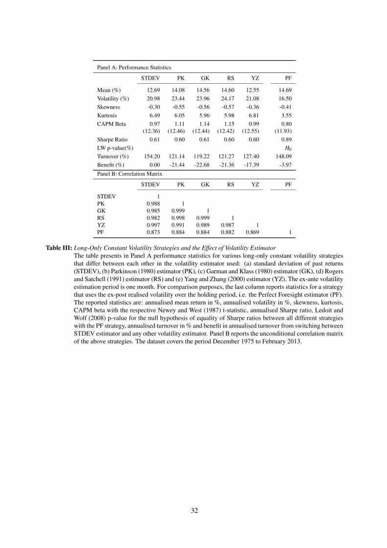
Panel A of Table III presents out-of-sample performance statistics for the long-only strategy using

various volatility estimators. The last column of the table reports these statistics for a hypothetical

strategy that uses the ex-post realised volatility to ex-ante scale the futures positions. This strategy

cannot be implemented in real-time and only constitutes a benchmark for the purpose of our analysis; for

that purpose, it is named the “perfect forecast” strategy (PF).

In terms of risk-adjusted returns, all strategies except for PF, deliver a Sharpe ratio of approximately

0.60, which means that the different volatility estimators do not have an economically significant effect

on the performance of the strategy before accounting for transaction costs. However, the annualised

turnover estimate for the strategy that uses conventional STDEV estimator drops by about one fifth

if one uses a more efficient range volatility estimator. This result supports our conjecture that more

efficient volatility estimators can significantly reduce the turnover of constant-volatility strategies hence

delivering greater risk-adjusted returns after accounting for transaction costs.

Comparing the results of implementable strategies to the PF benchmark, it is obvious that the strat-

egy with PF delivers greater risk-adjusted performance with a Sharpe ratio of 0.89, which is significantly

different from the Sharpe ratios of the rest of the strategies as deduced by the very low p-values of the

Ledoit and Wolf (2008) statistical test.10 The rejection of the null of equality in Sharpe ratios shows that

there is room of improvement in the form of superior volatility forecasts and in particular in the form

of forecasting unexpected increases in volatility and therefore better timing the downscaling of positions

before an impending drawdown. This task is beyond the objectives of this paper. Our main objective

is to show that increased estimation efficiency can significantly reduce the turnover and therefore the

transaction costs of a CVOL or TSMOM strategy and not to forecast future realised volatility. A word

of caution related to the latter task would be that a volatility forecast that can successfully predict un-

expected changes in volatility can lead to better ex-post performance, as shown by the PF results, but

at the same time, if predicted volatility changes do not end up realising themselves, this would lead to

excessive turnover and lower ex-post returns of the strategy.

[Table III about here]

Above we documented the advantage of superior volatility estimators for long-only CVOL strate-

gies. Next, we turn to the effect of different volatility estimators on the performance of the time-series

momentum strategies. Table IV shows that the choice of ex-ante volatility estimators does not have an10SETTINGS FOR LW TEST

13

economically important effect on the Sharpe Ratio (before transaction costs) which varies between 0.82

and 0.90. However, range-based volatility estimators reduce portfolio turnover by around a tenth. which

is likely to have a significant effect on after transaction cost performance.

[Table IV about here]

4.2.1. Robustness Tests - The Effect of Estimation Period

In Tables III and IV we studied the economic value of different volatility estimators based on the assump-

tion of a one month volatility estimation window. Next we examine whether the choice of the volatility

estimation window affects the marginal benefit of using the YZ estimator. Figures 3 and 4 report different

performance statistics and moments for estimation windows ranging from one to twelve months. They

also show the turnover benefit.


One of the key insights from Figure 4 is that the Sharpe ratio is maximised when using a three

month estimation window. Although this recommendation is empirically motivated, it lends support to

the choice of a three month volatility estimation window in Baltas and Kosowski (2013).


5. The Effect of Trading Signal

As discussed in the methodology section, the economic performance of a time-series momentum trading

strategy is chiefly driven by the volatility estimator and the choice of trading signal. In this section we

study two potential trading signals in detail and their effect on the performance of the trading strategy.

The two trading signals are return sign and time-trend t-statistic.

Return Sign (SIGN): The standard measure of past performance in the momentum literature as in

Moskowitz et al. (2012) and Baltas and Kosowski (2013) is the sign of the past 12-month past return. A

positive (negative) past return dictates a long (short) position:

SIGN(tm−12, tm) =

{+1, r (tm−12, tm)≥ 0

−1, otherwise(27)

Time-Trend t-statistic (TREND): Another way to capture the trend of a price series is through fitting a

linear trend on the past 12-month daily futures price series using least-squares. The momentum signal

can then be determined based on the significance of the slope coefficient of the fit. Assume the linear

regression model:

Fτ = α+βτ+ eτ, τ = 1, · · · , tm−12− tm (28)

14

The significance of the time-trend is determined by the t-statistic of β, t (β), and the cutoff points for the

long/short position of the trading signal are chosen to be +2/-2 respectively:

TREND(tm−12, tm) =

+1, if t(β)>+2

−1, if t(β)<−2

0, otherwise

(29)

In order to account for potential autocorrelation and heteroskedasticity in the price process, Newey and

West (1987) t-statistics are used.

5.1. Return Predictability

Following Moskowitz et al. (2012) and Baltas and Kosowski (2013), we next assess the amount of in-

sample return predictability that is inherent in lagged excess returns or lagged trading signals by running

the following pooled time-series cross-sectional regressions:

rxs, f c (tm−1, tm)σ(tm−2, tm−1)

= α+βλ

rxs, f c (tm−λ−1, tm−λ)

σ(tm−λ−2, tm−λ−1)+ ε(tm) (30)

andrxs, f c (tm−1, tm)σ(tm−2, tm−1)

= α+βλsignal (tm−λ−1, tm−λ)+ ε(tm) (31)

where λ denotes the lag that ranges between 1 and 60 months and the lagged signal (tm−λ−1, tm−λ) is

either SIGN(tm−λ−1, tm−λ) or TREND(tm−λ−1, tm−λ).

The regressions (30) and (31) is estimated for each lag by pooling together all Ti (where i = 1, · · · ,N)

monthly returns/trading signals for the N = 75 contracts. We are interested in the t-statistic of the coef-

ficient βλ for each lag. Large and significant t-statistics essentially support the hypothesis of time-series

return predictability. The t-statistics t (βλ) are computed using standard errors that are clustered by time

and asset,11 in order to account for potential cross-sectional dependence (correlation between contempo-

raneous returns of the contracts) or time-series dependence (serial correlation in the return series of each

individual contract). Briefly, the variance-covariance matrix of the regressions (30) and (31) is given by

(Cameron, Gelbach and Miller 2011, Thompson 2011):

VTIME&ASSET =VTIME +VASSET−VWHITE, (32)

where VTIME and VASSET are the variance-covariance matrices of one-way clustering across time and

asset respectively, and VWHITE is the White (1980) heteroscedasticity-robust OLS variance-covariance

matrix. In fact, Petersen (2009) shows that when T >> N (N >> T ) then standard errors computed via

one-way clustering by time (by asset) are close to the two-way clustered standard errors; nevertheless,

one-way clustering across the “wrong” dimension produces downward biased standard errors, hence

11Petersen (2009) and Gow, Ormazabal and Taylor (2010) study a series of empirical applications with panel datasets andrecognise the importance of correcting for both forms of dependence.

15

inflating the resulting t-statistics and leading to over-rejection rates of the null hypothesis. In our dataset,

not all assets have the same number of monthly observations. On average, we have T = 1N ∑

Ni=1 Ti ∼= 319

months of data per asset. We can therefore argue that T > N and we document that two-way clustering

or one-way clustering by time (i.e. estimating T cross-sectional regressions as in Fama and MacBeth

(1973)) produces similar results, whereas clustering by asset produces inflated t-statistics that are similar

to simple OLS t-statistics. Two-way clustering is also used by Baltas and Kosowski (2013), who study

the return predictability over monthly, weekly and daily frequencies, whereas one-way clustering by time

is used by Moskowitz et al. (2012).

Following the above, Figure 5 presents the two-way clustered t-statistics t (βλ) for regressions (30)

and (31) and lags λ = 1,2, · · · ,60 months. The t-statistics are almost always positive for the first twelve

months for all regressor choices, hence indicating strong momentum patterns of past year’s returns.

Moreover, the fact that the TREND signal is sparsely active does not seem to affect its return predictabil-

ity, which also remains statistically strong for the first twelve months. Apparently, it is the statistical

significance of the price trends that drive the documented momentum behaviour. Similarly to the evi-

dence in Moskowitz et al. (2012) and Baltas and Kosowski (2013), there exist statistically strong signs of

return reversals after the first year12 that subsequently attenuate and only seem to gain some significance

for a lag of around three years.


5.2. Performance Evaluation

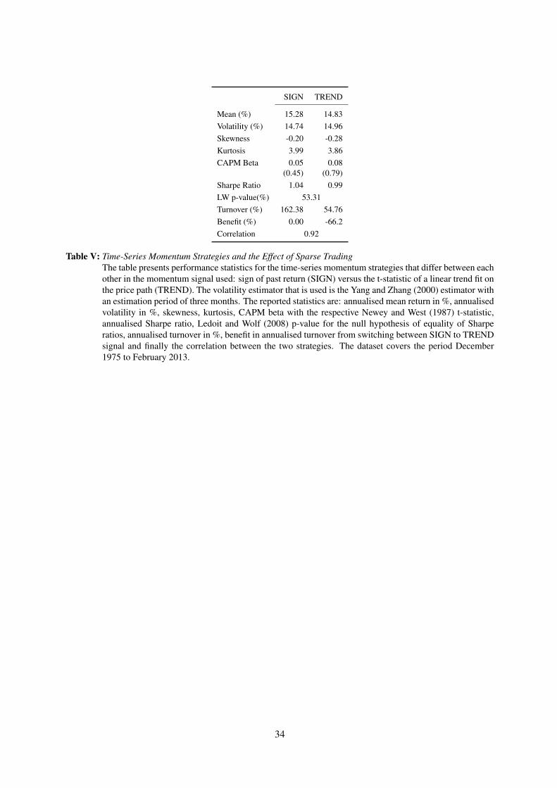
Similar to the analysis in Table IV, which studies the impact of the volatility estimator choice on turnover

and out of sample Sharpe ratio, in Table V we examine the economic value of using the SIGN or TREND

signal. It is clear from the table that the choice of the trading signal does not have an economically

significant impact on the Sharpe ratio before transaction costs. The Ledoit and Wolf (2008) p-value

shows that the Sharpe ratios of 1.04 and 0.99 are not statistically different from each other. However, the

choice of trading signal has a huge effect on turnover which for the TREND signal is about a third of that

resulting from the use of the SIGN signal. This implies that the TREND signal leads to a similar before

transaction cost Sharpe ratio, but only requires one third of the trading and associated cost.

[Table V about here]

So far we have analysed the economic value of using different signals on the time-series momentum

strategy portfolio. To gain a deeper understanding of the effect of trading signals in Figure 6 we study

the effect on the Sharpe ratio (before transaction costs) and turnover asset by asset. Panel A of Figure 6

12Part of this severe transition from largely positive and significant t-statistic to largely negative and significant t-statistic afterthe lag of twelve months can be potentially attributed to seasonal patterns in the commodity futures returns. In undocumentedresults, we repeat the pooled panel regression only on commodity contracts, after removing contracts that for various reasonsmight exhibit seasonality, like the agricultural and energy contracts. In general the patterns become relatively less pronounced,but our conclusions remain qualitatively the same and the momentum/reversal transition is still apparent

16

shows that the Sharpe ratio of each asset in blue and the change in the Sharpe ratio that would result

from the use of the TREND instead of the SIGN signal. Across all assets, on-average, the change is

insignificant as the TREND signal leads to an increase for some contracts and a decrease for others.

The reductions appear to be concentrated among fixed income and commodities contracts. Panel B of

Figure 6 shows the effect on turnover and supports earlier conclusions that using the TREND instead of

the SIGN signal has an economically large effect on performance net of transaction costs. The reduction

in turnover is around two thirds for most contracts but ranges from around 55 to around 85 percent.


To shed further light on the performance drivers of the time-series momentum strategy over time we

study the number of contracts that the strategy employs over time. Baltas and Kosowski (2013) show

that the time-series momentum strategy has the attractive feature of generating higher performance in

recessions rather than in booms. Therefore, we also examine when the strategy is net long or net short

on average across all contracts. Panel A of Figure 7 plots the number of contracts that are traded as a

result of using the SIGN or TREND signals. As we can see the TREND signal consistently leads to a

lower number of contracts employed and lower turnover. Panel B of Figure 7 shows that the time-series

momentum strategy tends to be on average more short in recessions than in booms independent of the

trading signal used. Panel B shows shows the net position (i.e. Long positions - Short positions/(sum

of absolute Long + absolute Short)). This results is not obvious since the investment opportunity set for

the strategy includes many futures contracts whose prices can be expected to be both pro and counter-

cyclical. However, it appears that many of the prices are pro-cyclical and by going short these assets in

recessions the time-series momentum strategy offers a hedge against an equity market downturn and thus

diversification benefits.


Apart form documenting the business cycle performance of the time-series momentum strategy,

Baltas and Kosowski (2013) also highlighted the decrease in the performance after 2008. Baltas and

Kosowski (2013) explain that the underperformance can be due to (i) capacity contracts, (ii) a lack of

trends for each asset or (iii) increase correlations across assets. The authors do not find evidence of

capacity constraints based on two different methodologies, but they do show that correlations between

futures markets have increased in the period from 2008 to 2013. To shed further light on this perfor-

mance decrease Panel A of Figure 8 shows the percentage of contracts for which the SIGN and TREND

have the same value (either 1 of -1). It illustrates that there is a drop at the end of the period which

implies that the TREND signal is likely to return more 0’s. Panel B of the figure shows the percentage

of TREND=0 contracts, i.e. contracts that show no signs of significant trend. We find that after 2008 the

number of contracts without a significant trend signal increases significantly and almost doubles. This is

one potential reason for the performance decrease in the time-series momentum strategy over time.


17

6. Concluding Remarks

The time-series momentum strategy refers to the trading strategy that results from the aggregation of

various univariate momentum strategies on a volatility-adjusted basis. Such strategies have received in-

creased attention after they again provided impressive diversification benefits during the recent financial

crisis in 2008 as in previous business cycle downturns. This paper builds on recent works by Moskowitz

et al. (2012) and Baltas and Kosowski (2013) that focus on the profitability of time-series momentum

strategies in futures markets and examines the effect of risk-weighting and choice of the trading signal on

the performance of time-series momentum strategies. In particular, we highlight the effect of the choice

of volatility estimator and trading signal on turnover and strategy performance.

We show that volatility adjustment of the constituents of the time-series momentum is critical for the

resulting portfolio turnover. The use of more efficient estimators like the Yang and Zhang (2000) range

estimator can substantially reduce the portfolio turnover and consequently the transaction costs for the

construction and rebalancing of the portfolio. Momentum trading signals generated by fitting a linear

trend on the asset price path maximise the out-of-sample performance while minimizing the portfolio

turnover, hence dominating other momentum trading signal commonly used in the literature.

Our results have important implications for portfolio construction and the practical implementation of

time-series momentum strategies. Future research on the appropriate sizing of the univariate time-series

momentum strategies, instead of ordinary volatility-adjusted aggregation, is potential and promising av-

enue for future research.

References

Alizadeh, S., Brandt, M. W. and Diebold, F. X.: 2002, Range-based estimation of stochastic volatility

models, Journal of Finance 57(3), 1047–1091.

Andersen, T. G., Bollerslev, T., Christoffersen, P. F. and Diebold, F. X.: 2006, Volatility and correlation

forecasting, Handbook of Econometric Forecasting 1, 777–878.

Baltas, A. N. and Kosowski, R.: 2013, Momentum strategies in futures markets and trend-following

funds, SSRN eLibrary .

Barber, B. M. and Odean, T.: 2000, Trading is hazardous to your wealth: The common stock investment

performance of individual investors, Journal of Finance 55(2), 773–806.

Barndorff-Nielsen, O. E. and Shephard, N.: 2002, Econometric analysis of realized volatility and its

use in estimating stochastic volatility models, Journal of the Royal Statistical Society: Series B,

Statistical Methodology 64(2), 253–280.

Barroso, P. and Santa-Clara, P.: 2013, Momentum has its moments, SSRN eLibrary .

18

Bessembinder, H.: 1992, Systematic risk, hedging pressure, and risk premiums in futures markets, Re-

view of Financial Studies 5(4), 637.

Bessembinder, H.: 1993, An empirical analysis of risk premia in futures markets, Journal of Futures

Markets 13(6), 611–630.

Brandt, M. W. and Kinlay, J.: 2005, Estimating historical volatility, Research Article, Investment Analyt-

ics .

Bryhn, A. C. and Dimberg, P. H.: 2011, An operational definition of a statistically meaningful trend,

PLoS ONE 6(4), e19241.

Cameron, A. C., Gelbach, J. B. and Miller, D. L.: 2011, Robust inference with multiway clustering,

Journal of Business and Economic Statistics 29(2), 238–249.

Daniel, K. and Moskowitz, T.: 2013, Momentum crashes, Columbia Business School Research Paper .

de Roon, F. A., Nijman, T. E. and Veld, C.: 2000, Hedging pressure effects in futures markets, Journal

of Finance 55(3), 1437–1456.

Dorn, D. and Huberman, G.: 2009, Turnover and volatility, working paper .

Fama, E. F. and MacBeth, J.: 1973, Risk and return: Some empirical tests, Journal of Political Economy

81, 607–636.

Fuertes, A., Miffre, J. and Rallis, G.: 2010, Tactical allocation in commodity futures markets: Combining

momentum and term structure signals, Journal of Banking and Finance 34(10), 2530–2548.

Garman, M. B. and Klass, M. J.: 1980, On the estimation of security price volatilities from historical

data, Journal of Business 53(1), 67–78.

Gorton, G. B., Hayashi, F. and Rouwenhorst, K. G.: 2007, The fundamentals of commodity futures

returns, NBER Working Paper .

Gorton, G. and Rouwenhorst, K. G.: 2006, Facts and fantasies about commodities futures, Financial

Analysts Journal 62(2), 47–68.

Gow, I. D., Ormazabal, G. and Taylor, D. J.: 2010, Correcting for cross-sectional and time-series depen-

dence in accounting research, The Accounting Review 85(2), 483–512.

Jegadeesh, N. and Titman, S.: 1993, Returns to buying winners and selling losers: Implications for stock

market efficiency., Journal of Finance 48(1), 65–91.

Jegadeesh, N. and Titman, S.: 2001, Profitability of momentum strategies: An evaluation of alternative

explanations, Journal of Finance 56(2), 699–720.

Karpoff, J. M.: 1987, The relation between price changes and trading volume: A survey, Journal of

Financial and Quantitative Analysis 22(1), 109–126.

19

Ledoit, O. and Wolf, M.: 2008, Robust performance hypothesis testing with the sharpe ratio, Journal of

Empirical Finance 15(5), 850–859.

Lo, A. W. and Wang, J.: 2009, Stock market trading volume, Handbook of Financial Econometrics

2, 241–356.

Luttmer, E.: 1996, Asset pricing in economies with frictions, Econometrica 64(6), 1439–1467.

Miffre, J. and Rallis, G.: 2007, Momentum strategies in commodity futures markets, Journal of Banking

and Finance 31(6), 1863–1886.

Moskowitz, T., Ooi, Y. H. and Pedersen, L. H.: 2012, Time series momentum, Journal of Financial

Economics 104(2), 228 – 250.

Newey, W. K. and West, K. D.: 1987, A simple, positive semi-definite, heteroskedasticity and autocorre-

lation consistent covariance matrix, Econometrica 55(3), 703–708.

Parkinson, M.: 1980, The extreme value method for estimating the variance of the rate of return, Journal

of Business 53(1), 61–65.

Pesaran, M., Schleicher, C. and Zaffaroni, P.: 2009, Model averaging in risk management with an appli-

cation to futures markets, Journal of Empirical Finance 16(2), 280–305.

Petersen, M. A.: 2009, Estimating standard errors in finance panel data sets: Comparing approaches,

Review of Financial Studies 22(1), 435.

Pirrong, C.: 2005, Momentum in futures markets, SSRN eLibrary .

Rogers, L. C. G. and Satchell, S. E.: 1991, Estimating variance from high, low and closing prices, Annals

of Applied Probability 1(4), 504–512.

Rogers, L. C. G., Satchell, S. E. and Yoon, Y.: 1994, Estimating the volatility of stock prices: a compar-

ison of methods that use high and low prices, Applied Financial Economics 4(3), 241–247.

Shu, J. and Zhang, J. E.: 2006, Testing range estimators of historical volatility, Journal of Futures

Markets 26(3), 297–313.

Thompson, S. B.: 2011, Simple formulas for standard errors that cluster by both firm and time, Journal

of Financial Economics 99(1), 1–10.

White, H.: 1980, A heteroskedasticity-consistent covariance matrix estimator and a direct test for het-

eroskedasticity, Econometrica 4, 817–838.

Yang, D. and Zhang, Q.: 2000, Drift-independent volatility estimation based on high, low, open, and

close prices, Journal of Business 73(3), 477–491.

20

STDEV PK GK RS YZ0

1

2

3

4

5Volatility Estimator Ranks (1: Best, 5: Worst)

Absolute Change in Reciprocal of VolatilityAbsolute Forecast Bias of Future RV

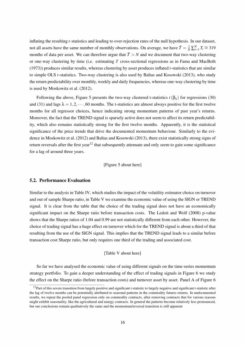
Figure 1: Volatility Estimator RanksThe bar chart presents the average rank (across 75 futures contracts) for five volatility estimators, withrespect to the absolute change in the reciprocal of estimated 1-month volatility and with respect to theforecast bias of future 1-month realized volatility. The volatility estimators are: (a) standard deviationof past returns (STDEV), (b) Parkinson (1980) estimator (PK), (c) Garman and Klass (1980) estimator(GK), (d) Rogers and Satchell (1991) estimator (RS) and (e) Yang and Zhang (2000) estimator (YZ). Thesample period of the dataset is December 1974 to February 2013; for the specific sample period of eachcontract see Table I.

21

−50

−40

−30

−20

−10

0

AU

D/U

SD

CA

D/U

SD

CH

F/U

SD

EU

R/U

SD

GB

P/U

SD

JPY

/US

DD

olla

r In

dex

DJI

AN

AS

DA

Q 1

00N

YS

E C

ompo

site

S&

P 5

00S

&P

400

Mid

Cap

Rus

sell

2000

DJ

Sto

xx 5

0E

uros

toxx

50

FT

SE

100

DA

XC

AC

40

IBE

X 3

5A

EX

SM

IM

IB 3

0S

&P

Can

ada

60N

ikke

i 225

TO

PIX

AS

X S

PI 2

00H

ang

Sen

gK

OS

PI 2

00M

SC

I Tai

wan

MS

CI E

AF

EU

S T

reas

ury

Bill

s 3

Mo

US

Tre

asur

y N

ote

2 Y

rU

S T

reas

ury

Not

e 5

Yr

US

Tre

asur

y N

ote

10 Y

rU

S T

reas

ury

Bon

d 30

Yr

Mun

icip

al B

onds

Eur

odol

lar

3 M

oE

urib

or 3

Mo

Eur

o/G

erm

an S

chat

z 2

Yr

Eur

o/G

erm

an B

obl 5

Yr

Eur

o/G

erm

an B

und

10 Y

rE

uro/

Ger

man

Bux

l 30

Yr

Aus

tral

ian

3 Y

rA

ustr

alia

n 10

Yr

UK

Ste

rling

3 M

oU

K L

ong

Gilt

Can

adia

n 10

Yr

Japa

nese

10

Yr

Kor

ean

3 Y

rLi

ght C

rude

Oil

Bre

nt C

rude

Oil

Hea

ting

Oil

Nat

ural

Gas

RB

OB

Gas

olin

eC

oppe

rG

old

Pal

ladi

umP

latin

umS

ilver

Fee

der

Cat

tleLi

ve C

attle

Live

Hog

sP

ork

Bel

lies

Cor

nO

ats

Soy

bean

Oil

Soy

bean

Mea

lS

oybe

ans

Whe

atC

ocoa

Cof

fee

Cot

ton

Lum

ber

Ora

nge

Juic

eS

ugar

Percentage drop in Absolute Change of Reciprocal of Volatility when switching from STDEV to YZ

%

INTEREST RATESEQUITIESFX COMMODITIES

Figure 2: Effect of Volatility Estimator choice on Reciprocal of VolatilityThe figure presents the percentage drop of the average absolute change in the reciprocal of volatility foreach of the 75 futures contracts of the dataset when switching from the standard deviation of past returns(STDEV) volatility estimator to the Yang and Zhang (2000) estimator (YZ). The specific sample periodof each contract is reported in Table I.

22

1 2 3 4 5 6 7 8 9 10 11 129.5

10

10.5

11

11.5

12

12.5

13

%

Annualised Mean Return

Months of Estimation1 2 3 4 5 6 7 8 9 10 11 12

0.53

0.54

0.55

0.56

0.57

0.58

0.59

0.6

0.61Sharpe ratio


0

20

40

60

80

100

120

140

%

Turnover

Months of Estimation

1 2 3 4 5 6 7 8 9 10 11 126

8

10

12

14

16

18

%

Turnover Benefit


−0.9

−0.8

−0.7

−0.6

−0.5

−0.4

−0.3

−0.2Skewness


5

5.5

6

6.5

7Kurtosis


Figure 3: Long-Only Constant Volatility Statistics for Different Estimation PeriodsThe figure presents the annualised mean return, the Sharpe ratio, the annualised turnover, the skewnessand the kurtosis of a long-only constant volatility strategy using Yang and Zhang (2000) volatility esti-mates across various estimation periods ranging between one to twelve past months. Additionally, theturnover benefit for switching from the standard deviation of past returns (STDEV) volatility estimator tothe Yang and Zhang (2000) estimator (this turnover benefit denotes a drop in the turnover, but is presentedas a positive number) is also presented.

23

1 2 3 4 5 6 7 8 9 10 11 1214

14.5

15

15.5

%

Annualised Mean Return


0.8

0.85

0.9

0.95

1

1.05Sharpe ratio


120

140

160

180

200

220

240

%

Turnover


1 2 3 4 5 6 7 8 9 10 11 120

2

4

6

8

10

12

%

Turnover Benefit


−2.5

−2

−1.5

−1

−0.5

0Skewness


0

5

10

15

20

25

30Kurtosis


Figure 4: Time-Series Momentum Statistics for Different Estimation PeriodsThe figure presents the annualised mean return, the Sharpe ratio, the annualised turnover, the skewnessand the kurtosis of a time-series momentum strategy using Yang and Zhang (2000) volatility estimatesacross various estimation periods ranging between one to twelve past months. Additionally, the turnoverbenefit for switching from the standard deviation of past returns (STDEV) volatility estimator to the Yangand Zhang (2000) estimator (this turnover benefit denotes a drop in the turnover, but is presented as apositive number) is also presented.

24

0 10 20 30 40 50 60−4

−2

0

2

4Return Level

Lag

0 10 20 30 40 50 60−4

−2

0

2

4SIGN

Lag

0 10 20 30 40 50 60−4

−2

0

2

4TREND

Lag

Figure 5: Time-Series Return PredictabilityThe figure presents the t-statistics of the pooled regression coefficient from regressing monthly excessreturns of the futures contracts on lagged excess returns or lagged excess momentum signals. Panel Apresents the results when lagged excess returns are used as the regressor, Panel B when the regressor isthe lagged SIGN signal and Panel C when the regressor is the lagged TREND signal. The t-statisticsare computed using standard errors clustered by asset and time (Cameron, Gelbach and Miller 2011,Thompson 2011). The volatility estimates are computed using the Yang and Zhang (2000) estimator ona one-month rolling window. The dashed lines represent significance at the 5% level. The dataset coversthe period December 1974 to February 2013.

25

−0.5

0

0.5

1Panel A: Sharpe ratios

SIGNChange due to TREND

−90

−80

−70

−60

−50

AU

D/U

SD

CA

D/U

SD

CH

F/U

SD

EU

R/U

SD

GB

P/U

SD

JPY

/US

DD

olla

r In

dex

DJI

AN

AS

DA

Q 1

00N

YS

E C

ompo

site

S&

P 5

00S

&P

400

Mid

Cap

Rus

sell

2000

DJ

Sto

xx 5

0E

uros

toxx

50

FT

SE

100

DA

XC

AC

40

IBE

X 3

5A

EX

SM

IM

IB 3

0S

&P

Can

ada

60N

ikke

i 225

TO

PIX

AS

X S

PI 2

00H

ang

Sen

gK

OS

PI 2

00M

SC

I Tai

wan

MS

CI E

AF

EU

S T

reas

ury

Bill

s 3

Mo

US

Tre

asur

y N

ote

2 Y

rU

S T

reas

ury

Not

e 5

Yr

US

Tre

asur

y N

ote

10 Y

rU

S T

reas

ury

Bon

d 30

Yr

Mun

icip

al B

onds

Eur

odol

lar

3 M

oE

urib

or 3

Mo

Eur

o/G

erm

an S

chat

z 2

Yr

Eur

o/G

erm

an B

obl 5

Yr

Eur

o/G

erm

an B

und

10 Y

rE

uro/

Ger

man

Bux

l 30

Yr

Aus

tral

ian

3 Y

rA

ustr

alia

n 10

Yr

UK

Ste

rling

3 M

oU

K L

ong

Gilt

Can

adia

n 10

Yr

Japa

nese

10

Yr

Kor

ean

3 Y

rLi

ght C

rude

Oil

Bre

nt C

rude

Oil

Hea

ting

Oil

Nat

ural

Gas

RB

OB

Gas

olin

eC

oppe

rG

old

Pal

ladi

umP

latin

umS

ilver

Fee

der

Cat

tleLi

ve C

attle

Live

Hog

sP

ork

Bel

lies

Cor

nO

ats

Soy

bean

Oil

Soy

bean

Mea

lS

oybe

ans

Whe

atC

ocoa

Cof

fee

Cot

ton

Lum

ber

Ora

nge

Juic

eS

ugar

Panel B: Percentage Drop in Turnover when switching from SIGN to TREND

%

Figure 6: The Effect of Sparse Trading SignalPanel A presents annualised Sharpe ratios for univariate time-series momentum strategies with 40%target volatility that use the SIGN of past return as trading signal. Additionally, the change in the Sharperatio from applying the TREND sparse trading signal is also presented. Panel B presents the percentagedrop in the turnover of each univariate strategy when switching between SIGN and TREND momentumsignals. The volatility estimator that is used across all strategies is the Yang and Zhang (2000) estimatorwith an estimation period of three months. The specific sample period of each contract is reported inTable I.

26

1975 1977 1979 1981 1983 1985 1987 1989 1991 1993 1995 1997 1999 2001 2003 2005 2007 2009 2011 20130

10

20

30

40

50

60

70

80Panel A: Number of Contracts with non−zero position

SIGNTREND

1975 1977 1979 1981 1983 1985 1987 1989 1991 1993 1995 1997 1999 2001 2003 2005 2007 2009 2011 2013−100

−50

0

50

100

%

Panel B: Net Position as Percentage of Available Contracts

SIGNTREND

Figure 7: Number of Contracts Traded and Net PositionsPanel A presents the number of contracts that are traded at the end of each month for the SIGN andTREND signals. The SIGN signal is always +1 or -1, hence the number of contracts traded for this signalequals the number of available contracts. Panel B presents the net position of the time-series momentumstrategy using the SIGN or the TREND signal. The net position is calculated as the sum of long contractsminus the sum of short contracts and then the result is expressed in percentage of the total number ofcontracts available at the end of each month. The sample period is December 1975 to February 2013.

27

1975 1977 1979 1981 1983 1985 1987 1989 1991 1993 1995 1997 1999 2001 2003 2005 2007 2009 2011 201370

75

80

85

90

%

Panel A: Percentage of Position Agreement between SIGN and TREND

1975 1977 1979 1981 1983 1985 1987 1989 1991 1993 1995 1997 1999 2001 2003 2005 2007 2009 2011 20135

10

15

20

25

%

Panel B: Fraction of Available Contracts with TREND=0

Figure 8: Comparison between SIGN and TREND SignalsPanel A presents the 12-month moving average of the percentage of contracts at the end of each monthfor which SIGN and TREND signals agree (i.e. both long or short for each and every contract). Panel Bpresents the 12-month moving average of the percentage of available contracts at the end of each monthfor which the TREND signal does not identify a significant upward or downward trend and is thereforeequal to zero. The lookback period for which the signals are generated is 12 months and the sampleperiod is December 1975 (first observation in December 1976 due to the 12-month moving average) toFebruary 2013.

28

Exchange From Mean t(Mean) Vol. Skew Kurt. SR

CURRENCIES

AUD/USD CME Feb-1987 5.07 2.11 11.67 -0.40 4.94 0.44CAD/USD CME Feb-1977 0.90 0.79 6.88 -0.31 8.12 0.13CHF/USD CME Dec-1974 0.77 0.36 12.55 0.05 3.81 0.06EUR/USD CME Dec-1974 0.58 0.30 11.37 -0.08 3.55 0.05GBP/USD CME Oct-1977 1.69 0.85 10.70 0.04 4.96 0.16JPY/USD CME Apr-1977 0.69 0.31 11.97 0.49 4.46 0.06Dollar Index ICE Aug-1989 -1.59 -0.84 8.75 0.43 3.83 -0.18

EQUITIES

DJIA CBOT Dec-1974 4.89 1.92 15.22 -0.47 5.37 0.32NASDAQ 100 CME Feb-1983 9.29 1.91 25.40 -0.31 4.29 0.37NYSE Composite ICE Dec-1974* 5.19 1.96 15.30 -0.58 5.22 0.34S&P 500 CME Dec-1974 5.76 2.20 15.35 -0.48 4.62 0.38S&P 400 MidCap CME Jul-1991 9.59 2.48 17.17 -0.69 5.14 0.56Russell 2000 ICE Feb-1988 7.06 1.75 19.17 -0.49 4.01 0.37DJ Stoxx 50 Eurex Jan-1987 3.74 1.01 16.49 -0.86 4.98 0.23Eurostoxx 50 Eurex Jan-1987 3.88 0.94 18.92 -0.64 4.38 0.21FTSE 100 NYSE Liffe Feb-1978 4.41 1.75 16.05 -0.76 5.76 0.28DAX Eurex Dec-1974 4.64 1.33 20.07 -0.48 5.00 0.23CAC 40 NYSE Liffe Aug-1987 3.88 0.88 20.64 -0.32 4.12 0.19IBEX 35 MEFF Feb-1987 4.92 1.10 22.23 -0.47 4.89 0.22AEX NYSE Liffe Feb-1983 4.81 1.19 20.33 -0.73 5.38 0.24SMI Eurex Aug-1988 6.18 1.66 16.68 -0.56 4.27 0.37MIB 30 BI Jan-1998 -0.56 -0.09 22.87 0.00 3.80 -0.02S&P Canada 60 MX Feb-1982 4.39 1.38 15.75 -0.68 5.85 0.28Nikkei 225 CME Dec-1974 0.60 0.19 19.45 -0.22 4.20 0.03TOPIX TSE Dec-1974 0.37 0.11 17.86 -0.18 4.53 0.02ASX SPI 200 ASX Jun-1992* 2.75 0.81 13.58 -0.66 3.70 0.20Hang Seng SEHK Dec-1974 13.01 2.82 28.73 -0.26 5.71 0.45KOSPI 200 KRX Feb-1990* 6.51 0.93 31.63 0.86 6.86 0.21MSCI Taiwan SGX Jan-1988 10.28 1.36 34.76 0.43 4.85 0.30MSCI EAFE NYSE Liffe Dec-1974 2.97 1.03 15.90 -0.58 5.32 0.19

INTEREST RATES

US Treasury Bills 3Mo CME Feb-1982* 1.01 2.91 1.44 1.14 8.96 0.70US Treasury Note 2Yr CBOT Feb-1991 1.65 3.73 1.75 0.28 3.44 0.95US Treasury Note 5Yr CBOT Aug-1988 3.23 3.56 4.23 0.05 3.66 0.76US Treasury Note 10Yr CBOT Feb-1983 4.82 3.77 6.90 0.15 3.98 0.70US Treasury Bond 30Yr CBOT Nov-1982 5.93 3.18 10.55 0.25 4.46 0.56Municipal Bonds CBOT Jul-1985* 5.57 3.30 8.04 -0.58 4.62 0.69Eurodollar 3Mo CME Jan-1982 1.19 3.61 1.52 1.09 8.26 0.78Euribor 3Mo NYSE Liffe Feb-1999 0.41 1.56 0.73 1.27 11.72 0.57Euro/German Schatz 2Yr Eurex Apr-1997 1.00 2.43 1.39 0.08 3.59 0.72Euro/German Bobl 5Yr Eurex Feb-1997 2.71 2.94 3.29 -0.02 2.70 0.83Euro/German Bund 10Yr Eurex Feb-1997 4.17 2.98 5.35 0.08 2.88 0.78Euro/German Buxl 30Yr Eurex Oct-2005 5.53 1.28 12.64 1.02 4.83 0.44Australian 3Yr ASX Aug-2001 0.47 1.25 1.08 0.45 2.88 0.43Australian 10Yr ASX Aug-2001 0.36 1.26 0.93 0.27 2.96 0.38UK Sterling 3Mo NYSE Liffe Aug-1998 0.75 2.33 0.92 1.72 12.55 0.82UK Long Gilt NYSE Liffe Aug-1998 2.96 1.82 5.97 0.28 3.59 0.50Canadian 10Yr MX May-1990 4.76 3.88 5.87 -0.04 3.23 0.81Japanese 10Yr TSE Aug-2003 1.75 2.02 2.99 -0.73 4.99 0.59Korean 3Yr KRX Sep-2003* 1.69 1.63 3.08 0.88 6.64 0.55

(Continued on next page)

29

(Continued from previous page)

Exchange From Mean t(Mean) Vol. Skew Kurt. SR

COMMODITIES

ENERGYLight Crude Oil NYMEX Feb-1987 13.22 1.71 34.13 0.40 5.46 0.39Brent Crude Oil NYMEX Sep-2003 15.45 1.22 31.37 -0.63 4.81 0.49Heating Oil NYMEX Feb-1984 13.53 2.09 33.75 0.49 4.84 0.40Natural Gas NYMEX Feb-1993 0.01 0.00 61.39 1.03 5.77 0.00RBOB Gasoline NYMEX Oct-1987 22.10 2.99 36.24 0.36 5.45 0.61

METALSCopper COMEX Jan-1990 9.47 1.48 26.45 -0.05 5.46 0.36Gold COMEX Feb-1984 1.88 0.72 15.42 0.31 4.12 0.12Palladium NYMEX Feb-1994 14.37 1.60 35.29 0.34 5.68 0.41Platinum NYMEX Aug-2003 11.83 1.19 27.03 -0.81 7.33 0.44Silver COMEX Jan-1984 2.71 0.56 27.80 0.26 4.17 0.10

MEATFeeder Cattle CME Feb-1978 2.46 1.04 14.52 -0.38 5.20 0.17Live Cattle CME Dec-1974 4.66 1.70 16.51 -0.13 4.39 0.28Live Hogs CME Dec-1974 3.32 0.83 25.57 -0.04 3.31 0.13Pork Bellies CME Dec-1974* 0.80 0.15 36.87 0.44 4.23 0.02

GRAINSCorn CBOT Aug-1982 -0.92 -0.19 25.95 0.64 6.02 -0.04Oats CBOT Aug-1982 -1.02 -0.16 34.68 2.76 25.57 -0.03Soybean Oil CBOT Aug-1982 2.26 0.48 26.29 0.58 6.13 0.09Soybean Meal CBOT Aug-1982 8.70 1.90 25.19 0.24 3.88 0.35Soybeans CBOT Aug-1982 4.43 1.08 23.53 0.13 4.13 0.19Wheat CBOT Aug-1982 -2.98 -0.68 25.47 0.36 4.92 -0.12

SOFTSCocoa ICE Aug-1986 -3.81 -0.76 29.17 0.58 4.14 -0.13Coffee ICE Feb-1987 -2.04 -0.26 37.86 1.00 5.69 -0.05Cotton ICE Feb-1987 1.42 0.24 26.01 0.28 3.78 0.05Lumber CME Dec-1974 -3.43 -0.68 29.17 0.29 3.67 -0.12Orange Juice ICE Aug-1987 2.87 0.47 32.25 0.68 4.57 0.09Sugar ICE Aug-1986 8.77 1.34 33.10 0.33 3.81 0.27

Table I: Summary Statistics for Futures ContractsThe table presents summary statistics for the 75 futures contracts of the dataset, which are estimated usingmonthly fully collateralised excess return series. The statistics are: annualised mean return in %, Neweyand West (1987) t-statistic, annualised volatility in %, skewness, kurtosis and annualised Sharpe ratio (SR).The table also indicates the exchange that each contract is traded at the end of the sample period as wellas the starting month and year for each contract. All but 7 contracts have data up until February 2013.The remaining 7 contracts are indicated by an asterisk (*) next to the starting date and their sample endsprior to February 2013: NYSE Composite up to January 2012, ASX SPI 200 up to January 2012, KOSPI200 up to January 2012, US Treasury Bills 3Mo up to August 2003, Municipal Bonds up to March 2006,Korean 3Yr up to June 2011 and Pork Bellies up to April 2011. The EUR/USD contract is spliced withthe DEM/USD (Deutche Mark) contract for dates prior to January 1999 and the RBOB Gasoline contractis spliced with the Unleaded Gasoline contract for dates prior to January 2007, following Moskowitz, Ooiand Pedersen (2012). The exchanges that appear in the table are listed next: CME: Chicago MercantileExchange, CBOT: Chicago Board of Trade, ICE: IntercontinentalExchange, Eurex: European Exchange,NYSE Liffe: New York Stock Exchange / Euronext - London International Financial Futures and OptionsExchange, MEFF: Mercado Espanol de Futuros Financieros, BI: Borsa Italiana, MX: Montreal Exchange,TSE: Tokyo Stock Exchange, ASX: Australian Securities Exchange, SEHK: Hong Kong Stock Exchange,KRX: Korea Exchange, SGX: Signapore Exchange, NYMEX: New York Mercantile Exchange, COMEX:Commodity Exchange, Inc.

30

Range Estimator Drift of diffusion process Overnight Jump Efficiency vs. STDEV

Parkinson (1980) Assumes zero drift Assumes no jump 5.2xGarman and Klass (1980) Assumes zero drift Assumes no jump 7.4xRogers and Satchell (1991) Allows for non-zero drift Assumes no jump 6.2xYang and Zhang (2000) Allows for non-zero drift Allows for jump 8.2x (21-day estimator)

Table II: Theoretical Features of Range Volatility EstimatorsThe table presents the theoretical features for four range volatility estimators: Parkinson (1980) estimator,(b) Garman and Klass (1980) estimator, (c) Rogers and Satchell (1991) estimator and (d) Yang and Zhang(2000) estimator.

31

Panel A: Performance Statistics

STDEV PK GK RS YZ PF

Mean (%) 12.69 14.08 14.56 14.60 12.55 14.69Volatility (%) 20.98 23.44 23.96 24.17 21.08 16.50Skewness -0.30 -0.55 -0.56 -0.57 -0.36 -0.41Kurtosis 6.49 6.05 5.96 5.98 6.81 3.55CAPM Beta 0.97 1.11 1.14 1.15 0.99 0.80

(12.36) (12.46) (12.44) (12.42) (12.55) (11.93)Sharpe Ratio 0.61 0.60 0.61 0.60 0.60 0.89LW p-value(%) H0

Turnover (%) 154.20 121.14 119.22 121.27 127.40 148.09Benefit (%) 0.00 -21.44 -22.68 -21.36 -17.39 -3.97

Panel B: Correlation Matrix


STDEV 1PK 0.988 1GK 0.985 0.999 1RS 0.982 0.998 0.999 1YZ 0.997 0.991 0.989 0.987 1PF 0.873 0.884 0.884 0.882 0.869 1

Table III: Long-Only Constant Volatility Strategies and the Effect of Volatility EstimatorThe table presents in Panel A performance statistics for various long-only constant volatility strategiesthat differ between each other in the volatility estimator used: (a) standard deviation of past returns(STDEV), (b) Parkinson (1980) estimator (PK), (c) Garman and Klass (1980) estimator (GK), (d) Rogersand Satchell (1991) estimator (RS) and (e) Yang and Zhang (2000) estimator (YZ). The ex-ante volatilityestimation period is one month. For comparison purposes, the last column reports statistics for a strategythat uses the ex-post realised volatility over the holding period, i.e. the Perfect Foresight estimator (PF).The reported statistics are: annualised mean return in %, annualised volatility in %, skewness, kurtosis,CAPM beta with the respective Newey and West (1987) t-statistic, annualised Sharpe ratio, Ledoit andWolf (2008) p-value for the null hypothesis of equality of Sharpe ratios between all different strategieswith the PF strategy, annualised turnover in % and benefit in annualised turnover from switching betweenSTDEV estimator and any other volatility estimator. Panel B reports the unconditional correlation matrixof the above strategies. The dataset covers the period December 1975 to February 2013.

32

Panel A: Performance Statistics


Mean (%) 14.95 17.95 18.23 18.33 14.72 17.33Volatility (%) 17.96 19.95 20.27 20.39 17.91 13.34Skewness -2.38 -1.93 -1.88 -1.83 -2.31 -0.03Kurtosis 27.88 21.80 20.87 20.35 26.79 3.02CAPM Beta 0.07 0.06 0.06 0.06 0.08 0.02

(0.66) (0.51) (0.50) (0.49) (0.68) (0.21)Sharpe Ratio 0.83 0.90 0.90 0.90 0.82 1.30LW p-value(%) H0

Turnover (%) 250.14 219.49 217.79 219.67 225.00 243.42Benefit (%) 0.00 -12.25 -12.93 -12.18 -10.05 -2.68

Panel B: Correlation Matrix


STDEV 1PK 0.990 1GK 0.988 0.999 1RS 0.986 0.999 1 1YZ 0.997 0.992 0.992 0.991 1PF 0.833 0.850 0.852 0.853 0.838 1

Table IV: Time-Series Momentum Strategies and the Effect of Volatility EstimatorThe table presents in Panel A performance statistics for various time-series momentum strategies that dif-fer between each other in the volatility estimator used: (a) standard deviation of past returns (STDEV),(b) Parkinson (1980) estimator (PK), (c) Garman and Klass (1980) estimator (GK), (d) Rogers andSatchell (1991) estimator (RS) and (e) Yang and Zhang (2000) estimator (YZ). The ex-ante volatilityestimation period is one month. For comparison purposes, the last column reports statistics for a strategythat uses the ex-post realised volatility over the holding period, i.e. the Perfect Foresight estimator (PF).The reported statistics are: annualised mean return in %, annualised volatility in %, skewness, kurtosis,CAPM beta with the respective Newey and West (1987) t-statistic, annualised Sharpe ratio, Ledoit andWolf (2008) p-value for the null hypothesis of equality of Sharpe ratios between all different strategieswith the PF strategy, annualised turnover in % and benefit in annualised turnover from switching betweenSTDEV estimator and any other volatility estimator. Panel B reports the unconditional correlation matrixof the above strategies. The dataset covers the period December 1975 to February 2013.

33

SIGN TREND

Mean (%) 15.28 14.83Volatility (%) 14.74 14.96Skewness -0.20 -0.28Kurtosis 3.99 3.86CAPM Beta 0.05 0.08

(0.45) (0.79)Sharpe Ratio 1.04 0.99LW p-value(%) 53.31Turnover (%) 162.38 54.76Benefit (%) 0.00 -66.2Correlation 0.92

Table V: Time-Series Momentum Strategies and the Effect of Sparse TradingThe table presents performance statistics for the time-series momentum strategies that differ between eachother in the momentum signal used: sign of past return (SIGN) versus the t-statistic of a linear trend fit onthe price path (TREND). The volatility estimator that is used is the Yang and Zhang (2000) estimator withan estimation period of three months. The reported statistics are: annualised mean return in %, annualisedvolatility in %, skewness, kurtosis, CAPM beta with the respective Newey and West (1987) t-statistic,annualised Sharpe ratio, Ledoit and Wolf (2008) p-value for the null hypothesis of equality of Sharperatios, annualised turnover in %, benefit in annualised turnover from switching between SIGN to TRENDsignal and finally the correlation between the two strategies. The dataset covers the period December1975 to February 2013.

34

Date post:	26-Apr-2018
Category:	Documents
Upload:	trinhtuyen
View:	214 times
Download:	1 times

Improving Time-Series Momentum Strategies: The Role of ... · †Corresponding Author; (i) UBS...

Documents