Improving Word Similarity by Augmenting PMI with Estimates of Word Polysemy

Improving Word Similarity by AugmentingPMI with Estimates of Word Polysemy

Lushan Han, Tim Finin, Paul McNamee,

Anupam Joshi, and Yelena Yesha, Member, IEEE Computer Society

Abstract—Pointwise mutual information (PMI) is a widely used word similarity measure, but it lacks a clear explanation of how it

works. We explore how PMI differs from distributional similarity, and we introduce a novel metric, PMImax, that augments PMI with

information about a word’s number of senses. The coefficients of PMImax are determined empirically by maximizing a utility function

based on the performance of automatic thesaurus generation. We show that it outperforms traditional PMI in the application of

automatic thesaurus generation and in two word similarity benchmark tasks: human similarity ratings and TOEFL synonym questions.

PMImax achieves a correlation coefficient comparable to the best knowledge-based approaches on the Miller-Charles similarity rating

data set.

Index Terms—Semantic similarity, pointwise mutual information, automatic thesaurus generation, corpus statistics

Ç

1 INTRODUCTION

WORD similarity is a measure of how semanticallysimilar a pair of words is, with synonyms having the

highest value. It is widely used for applications in naturallanguage processing (NLP), information retrieval (IR), andartificial intelligence, including tasks like word sensedisambiguation [1], malapropism detection [2], paraphraserecognition [3], image and document retrieval [4] andpredicting hyperlink-following behavior [5]. There are twoprevailing approaches to computing word similarity, basedon either using of a thesaurus (e.g., WordNet [6]) orstatistics from a large corpus. There are also hybridapproaches [7] combining the two methods. Many well-known word similarity measures have been based onWordNet [8], [9], [10] and most of semantic applications[1], [4], [2] rely on these taxonomy-based measures.

Organizing all words in a well-defined taxonomy andlinking them together with different relations is a labor-intensive task that requires significant maintenance as newwords and word senses are formed. Furthermore, existingWordNet-based similarity measures typically depend heav-ily on “IS-A” information, which is available for nouns butincomplete for verbs and completely lacking for adjectivesand adverbs. Consequently, these metrics perform poorly(with accuracy no more than 25 percent) [11] in answeringTest of English as a Foreign Language (TOEFL) synonym

questions [12] where the goal is selecting which of fourcandidate choices is most like a synonym to a given word.In contrast, some corpus-based approaches achieve muchhigher accuracy on the task (above 80 percent) [13], [14].

We expect statistical word similarity to continue to playan important role in semantic acquisition from text [9] in thefuture. A common immediate application is automaticthesaurus generation, in which various statistical wordsimilarity measures [15], [16], [17], [18], [19] have beenproposed. These are based on the distributional hypothesis[20], which states that words occurring in the same contextstend to have similar meanings. Thus, the meaning of a wordcan be represented by a context vector of accompanyingwords and their co-occurrences counts, modulated perhapsby weighting functions [18], measured either in documentcontext, text window context, or grammatical dependencycontext. The context vectors can be further transformed to aspace of reduced dimension by applying singular valuedecomposition (SVD), yielding the familiar latent semanticanalysis (LSA) technique [12]. The similarity of two wordsis then computed as the similarity of their context vectors,and the most common metric is the cosine of the anglebetween the two vectors. We will refer this kind of wordsimilarity as distributional similarity, following conventionin the research community [21], [22], [2].

PMI has emerged as a popular statistical word similaritymeasure that is not based on the distributional hypothesis.Calculating PMI only requires simple statistics about twowords: their marginal frequencies and their co-occurrencefrequency in a corpus. In the ten years after PMI wasintroduced to statistical NLP by Church and Hanks [23], itwas mainly used for measuring word association [24] andwas not thought of as a word similarity measure. Alongwith other statistical association measures such as the t-test,�2-test, and likelihood ratio, PMI was commonly used forfinding collocations [24]. PMI was also a popular weightingfunction used in computing distributional similarity mea-sures [15], [17], [22]. Using PMI as a word similaritymeasure began with the work of Turney [25], whodeveloped a technique he called PMI-IR that used page

IEEE TRANSACTIONS ON KNOWLEDGE AND DATA ENGINEERING, VOL. 25, NO. 6, JUNE 2013 1307

. L. Han, T. Finin, A. Joshi, and Y. Yesha are with the Department ofComputer Science and Electrical Engineering, University of Maryland,Baltimore County, 1000 Hilltop Circle, Baltimore, MD 21250.E-mail: [email protected],{finin, joshi}@cs.umbc.edu, [email protected].

. P. McNamee is with the Applied Physics Laboratory and the HumanLanguage Technology Center of Excellence, Johns Hopkins University,810 Wyman Park Drive, Baltimore, MD 21211-2840.E-mail: [email protected].

Manuscript received 13 Mar. 2011; revised 3 Oct. 2011; accepted 6 Jan. 2012;published online 13 Feb. 2012.Recommended for acceptance by P. Ipeirotis.For information on obtaining reprints of this article, please send e-mail to:[email protected], and reference IEEECS Log Number TKDE-2011-03-0124.Digital Object Identifier no. 10.1109/TKDE.2012.30.

1041-4347/13/$31.00 � 2013 IEEE Published by the IEEE Computer Society

counts from a web search engine to approximate frequencycounts in computing PMI values for word pairs. Thisproduced remarkably good performance in answeringTOEFL synonym questions—an accuracy of 74 percentwhich outperformed LSA [12], and was the best result atthat time.

Turney’s result was surprising because finding syno-nyms was a typical task for distributional similaritymeasures, and PMI, a word association measure, per-formed even better. Terra and Clarke [13] redid the TOEFLexperiments for a set of the most well-known wordassociation measures including PMI, �2-test, likelihoodratio, and average mutual information. The experimentswere based on a very large web corpus, and documentand text window contexts of various sizes were investi-gated. They found PMI performed the best overall, andobtained an accuracy of 81.25 percent with a window sizeof 16 to 32 words.

PMI-IR has subsequently been used as a word similaritymeasure in other applications with good results. Mihalceaet al. [3] used PMI-IR, LSA, and six WordNet-based similaritymeasures as a submodule in computing text similarity andapplying it to paraphrase recognition and found that PMI-IRslightly outperformed the others. In a task of predicting userclick behavior, predicting the HTML hyperlinks that a user ismost likely to select given an information goal, Kaur andHornof [5] also showed that PMI-IR performs better than LSAand six WordNet-based measures.

Why PMI is effective as a word similarity measure is stillnot clear. Many researchers use Turney’s good results ofPMI-IR as empirical credence [13], [26], [3], [5], [27]. Toexplain the success of PMI, some propose the proximityhypothesis [26], [13] noting that similar words tend to occurnear each other, which is quite different from the distribu-tional hypothesis which assumes that similar words tend tooccur in similar contexts. However, to our knowledge, nofurther explanations have been provided in the literature.

In this paper, we offer an intuitive explanation for whyPMI can be used as a word similarity measure and illustratebehavioral differences between first-order PMI similarityand second-order distributional similarity. We also providenew experiments and examples, allowing more insight intoPMI similarity. Our main contribution is introducing anovel metric, PMImax, that enhances PMI to take intoaccount the fact that words have multiple senses. The newmetric is derived from the assumption that more frequentcontent words have more senses. We show that PMImaxsignificantly improves the performance of PMI in theapplication of automatic thesaurus generation and outper-forms PMI on benchmark data sets including humansimilarity rating data sets and TOEFL synonym questions.PMImax also has the advantage of not requiring expensiveresources, such as sense-annotated corpora.

The remainder of the paper proceeds as follows: InSection 2, we discuss PMI similarity and define the PMImaxmetric. In Section 3, we use experiments in automaticthesaurus generation to determine the coefficients ofPMImax, evaluate its performance, and examine its assump-tions. Additional evaluation using benchmark data sets ispresented in Section 4. Section 5 discusses potentialapplications of PMImax and our future work. We areparticularly interested in exploiting behavioral differences

between PMI similarity and distributional similarity in theapplication of semantic acquisition from text. Finally, weconclude the paper in Section 6.

2 APPROACH

We start this section by discussing why PMI can serve as asemantic similarity measure. Then, we point out a problemintroduced by PMI’s assumption that words only possess asingle sense, and we propose a novel PMI metric to considerpolysemy of words.

2.1 PMI as a Semantic Similarity Measure

Intuitively, the semantic similarity between two concepts1

can be defined as how much commonality they share. Sincethere are different ways to define commonality, semanticsimilarity tends to be a fuzzy concept. Is soldier more similarto astronomer or to gun? If commonality is defined as purelyinvolving IS-A relations in a taxonomy such as WordNet,then soldier would be more similar to astronomer becauseboth are types of people. But if we base commonality onaptness to a domain, then soldier would be more similar togun. People naturally do both types of reasoning, and toevaluate computational semantic similarity measures, thestandard practice is to rely on subjective human judgments.

Many researchers think that semantic similarity ought tobe based only on IS-A relations and that it represents aspecial case of semantic relatedness which also includesantonymy, meronymy, and other associations [2]. However,in the literature, semantic similarity also refers to the notionof belonging to the same semantic domain or topic, and isinterchangeable with semantic relatedness or semanticdistance [24]. In this paper, we take the more relaxed viewand use two indicators to assess the goodness of a statisticalword similarity measure: 1) its ability to find synonyms,and 2) how well it agrees with human similarity ratings.

We use Nida’s example noted by Lin [17] to helpdescribe why PMI can be a semantic similarity measure:

A bottle of tezguino is on the table.

Everyone likes tezguino.

Tezguino makes you drunk.

We make tezguino out of corn.

By observing the contexts in which the concept tezguinois used, we can infer that tezguino is a kind of alcoholicbeverage made from corn, exemplifying the idea that aconcept’s meaning can be characterized by its contexts. Bysaying a concept has a context, we mean the concept islikely to appear in the context. For example, tezguino islikely to appear in the context of “drunk,” so tezguino hasthe context “drunk.” We may then define concept similarityas how much their contexts overlap, as illustrated in Fig. 1.The larger the overlap becomes, the more similar the twoconcepts are, and vice versa.

Two concepts are more likely to co-occur in a common,shared context and less likely in an unshared one. In ashared context, both have an increased probability ofappearing but in an unshared one, as in Fig. 1, one is more

1308 IEEE TRANSACTIONS ON KNOWLEDGE AND DATA ENGINEERING, VOL. 25, NO. 6, JUNE 2013

1. A concept refers to a particular sense of a word and we use an italicword to signify it in this section.

likely but the other not. Generally, for two concepts withfixed sizes,2 the larger their context overlap is, the more co-occurrences result. In turn, the number of co-occurrencescan be used to indicate the amount of common contextsbetween two concepts with fixed sizes.

The number of co-occurrences also depends on the sizesof the two concepts. Therefore, we need a normalizedmeasure of co-occurrences to represent their similarity. PMIfits this role well. Equation (1) shows how to compute PMIfor concepts in a sense-annotated text corpus, where fc1

andfc2

are the individual frequencies (counts) of the twoconcepts c1 and c2 in the corpus, and fdðc1; c2Þ is the co-occurrence frequency of c1 and c2 measured by the contextwindow of dwords andN is the total number of words in thecorpus. In this paper, log always stands for natural logarithm

PMIðc1; c2Þ � logfdðc1; c2Þ �Nfc1� fc2

� �: ð1Þ

Traditionally, PMI is explained as the logarithmic ratio ofthe actual joint probability of two events to the expectedjoint probability if the two events were independent [23].Here, we interpret it from a slightly different perspectiveand this interpretation is used in deriving our novel PMImetric in the next section. The term fc1

� fc2can be

interpreted as the number of all co-occurrence possibilitiesor combinations between c1 and c2.3 The term fdðc1; c2Þ givesthe number of co-occurrences actually fulfilled. Thus, theratio fdðc1;c2Þ

fc1 �fc2measures the extent to which two concepts tend

to co-occur. By analogy to the correlation in statistics whichmeasures the degree that two random variables tend to co-increase/decrease, PMI measures the likelihood that twoconcepts tend to co-occur versus occurring alone. In thissense, we say that PMI computes the correlation betweenthe concepts c1 and c2. We also refer to the semanticsimilarity that PMI represents as correlation similarity.

Because a concept has the largest context overlap withitself, a concept has the largest chance to co-occur withitself. In other words, a concept has the strongest correlationwith itself (autocorrelation). Autocorrelation is closelyrelated to word burstiness, a phenomenon that words tendto appear in bursts. If the “one sense per discourse”hypothesis [28] is applied, word burstiness would beessentially the same as concept burstiness. Thus, wordburstiness is a reflection of the autocorrelation of concepts.

It is interesting that synonym correlation derives fromthe autocorrelation of concepts. If identical concepts happenwithin a distance as short as a few sentences, writers oftenprefer using synonyms to avoid excessive lexical repetition.The probability of substituting synonyms depends on thenature of the concept as well as the writer’s literary style. Inour observations, synonym correlation often has a valuevery close to autocorrelation for verb, adjective, and adverbconcepts, but a value a little bit lower for nominal concepts.One reason may be the ability to use a pronoun as analternative to a synonym in English. Although verbs,adjectives, and adverbs also have pronominal forms, theyare less powerful than pronouns and used less frequently.

PMI similarity is related to distributional similarity inthat both are context-based similarity measures. However,they use contexts differently which results in differentbehaviors. First, the PMI similarity between two concepts isdetermined by how much their contexts overlap, whiledistributional similarity depends on the extent that twoconcepts have similar context distributions. For example,garage has a very high PMI similarity with car because garagerarely occurs in contexts which are not subsumed by thecontexts of car. However, distributional similarity typicallydoes not consider garage to be very similar to car because thecontext distributions of garage and car vary considerably.While one might expect all words related by a PART-OFrelation to have high PMI similarity, this is not the case.Table is not PMI-similar to leg, because there are many othercontexts related to leg but not table, and vice versa.

Second, for two given concepts, distributional similarityobtains collective contextual information for each conceptand computes how similar their context vectors are. Fordistributional similarity, it does not require the concepts toco-occur in the same contexts to be similar. In contrast, PMIsimilarity emphasizes the propensity for two concepts to co-occur in the exactly same contexts. For example, thedistributional similar concepts for car may include not onlyautomobile, truck, and train, but also boat, ship, carriage, andchariot. This shows the ability of distributional similarity tofind “indirect” similarity. However, a problem with dis-tributional similarity is that it cannot distinguish them andseparate them into three categories: “land vehicle,” “watervehicle,” and “archaic vehicle.” On the other hand, the PMI-similar concepts for car do not contain boat or carriagebecause they do not co-occur with car in the same contextsfrequently enough.

These differences suggest that PMI similarity should be avaluable complement to distributional similarity. Althoughthe idea that PMI can complement distributional similarityis not new, current techniques [29], [27] have used them asseparate features in statistical models and do not exploithow that they differ. In Section 5, we will show throughexamples that we can support interesting applications byexploiting their behavioral differences.

2.2 Augmenting PMI to Account for Polysemy

Since it is very expensive to produce a large sense-taggedcorpus, statistical semantic similarity measures are oftencomputed based on words rather than word senses [2].However, when PMI is applied to measure correlationbetween words,4 it has a problem because it assumes that

HAN ET AL.: IMPROVING WORD SIMILARITY BY AUGMENTING PMI WITH ESTIMATES OF WORD POLYSEMY 1309

2. The size of a concept refers to the frequency count of the concept in acorpus.

3. The requirement for multiplication rather than addition can be easilyunderstood by an example: if one individual frequency increased twofold,all co-occurrence possibilities would be doubled rather than increased bythe individual frequency.

4. The same formula as in (1) is used, except that senses are replaced bywords.

Fig. 1. Common contexts between concepts A and B.

words only have a single sense. Consider “make” and“earn” as an example. “Make” has many senses, only one ofwhich is synonymous with “earn,” and so it is inappropri-ate to divide by the whole frequency of “make” incomputing the PMI correlation similarity between “make”and “earn,” since only a fraction of “make” occurrenceshave the same meaning of “earn.”

PMI has a well-known problem that it tends to over-emphasize the association of low frequency words [30], [31],[32]. We conjecture that the fact that more frequent contentwords tend to have more senses, as shown in Fig. 4, is animportant cause for PMI’s frequency bias. More frequentwords are disadvantaged in producing high PMI valuebecause they tend to have more unrelated or less relatedsenses and thereby bear an extra burden by including thefrequencies of these senses in their marginal counts. Weshould distinguish this cause from the one described byDunning [33] that the normality assumption breaks downon rare words, which can be ruled out by using a minimumfrequency threshold.

Although it can be difficult to determine which sense of aword is being used, this does not prevent us from making amore accurate assumption than the “single sense” assump-tion. We will demonstrate a significant improvement overtraditional PMI by merely assuming that more frequentcontent words have a greater number of senses.

We start by modeling the number of the senses of anopen-class word (i.e., noun, verb, adjective, or adverb) as apower function of the log frequency of the word with ahorizontal translation q. More specifically,

yw ¼ aðlogðfwÞ þ qÞp; ð2Þ

where fw and yw are the frequency (count) of the word wand its number of senses, respectively; a, p, and q are threecoefficients needed to resolve. The displacement q isnecessary because fw is not a normalized measure of theword w and varies on the size of the selected corpus. Werequire ðlogðfwÞ þ q > 0Þ to only take the strict monotoneincreasing part of the power function. The power functionassumption is based on observing the graphs in Fig. 4,which show the dependence between a word’s logfrequency in a large corpus (e.g., two billion words) andits number of senses obtained from WordNet. This relation-ship, though simple, is better modeled using a powerfunction rather than a linear one.

We next estimate a word pair’s PMI value between theirclosest senses using two assumptions. Given a word pair, itis hard to know the proportions at which the closest sensesare engaged in their own words. Since it can be either amajor or minor sense, we simply assume the averageproportion 1

yw. Consequently, the frequency of a word used

as the sense most correlated with a sense in the other wordis estimated as fw

yw.

The co-occurrence frequency between a word pair w1

and w2, represented by fdðw1; w2Þ, is also larger than the co-occurrence frequency between the two particular senses ofw1 and w2. To estimate the co-occurrence frequencybetween the two senses, we assume that w1 and w2 havestrongest correlation only on the two particular senses andotherwise normal correlation. Normal correlation is theexpected correlation between common English words and

we denote it using PMI value k.5 Therefore, the co-occurrence frequency between the two particular senses ofw1 and w2 can be estimated by subtracting the co-occurrence frequency contributed by other combinationsof senses, denoted by x, from the total co-occurrencefrequency between the two words. More specifically,

fdðw1; w2Þ � x;

where x is computed using the definition of PMI by solving

logx �N

fw1� fw2

� fw1

yw1� fw2

yw2

0@

1A ¼ k: ð3Þ

Equation (3) amounts to asking the question—with acorrelation degree of k, how many co-occurrences areexpected among the remaining co-occurrence possibilitiesresulted by excluding the possibilities between the twosenses of interest from the total possibilities.

Finally, the modified PMI, called PMImax, between thetwo words w1 and w2 is given in

PMImaxðw1; w2Þ

¼ log ðfdðw1;w2Þ�xÞ�Nfw1yw1�fw2yw2

!

¼ log

�fdðw1;w2Þ�e

k

N ��fw1�fw2�fw1yw1�fw2yw2

��N

fw1yw1�fw2yw2

!:

ð4Þ

PMImax estimates the maximum correlation between twowords, i.e., the correlation between their closest senses. Incircumstances where we cannot know the particular sensesused, it is reasonable to take the maximum similarityamong all possible sense pairs as a measure of wordsimilarity. For example, when sense information is unavail-able, the shortest path assumption is often taken to computeword similarity in the WordNet-based measures. While theassumptions made in deriving the PMImax may appearnaive, we will demonstrate their effectiveness in latersections. More sophisticated models may lead to betterresults and we plan to explore this in future work.

3 EXPERIMENTS

In this section, we determine values for the coefficients usedin PMImax by selecting ones that maximize performance inautomatic thesaurus generation, where the core task is tofind synonyms for a target word. Synonyms can besynonymous to the target word in their major or minorsenses, and synonyms with more senses tend to be moredifficult to find because they have relatively less semanticoverlap with the target. Because more frequent words tendto have more senses, the synonyms underweighted by PMIare often those with high frequency. We hope PMImax canfix or alleviate this problem and find synonyms without afrequency bias.

Since word similarity is usually measured within thesame part of speech (POS) (e.g., in [8], [9], [10]), we learndifferent coefficient sets for nouns, verbs, adjectives, and


5. More explanations will be given in Section 3.4 after k is empiricallylearned and exhibited in Table 5.

adverbs. We further examine the learned relations betweenthe frequency of a word with a particular POS and itsnumber of senses within the POS (i.e., (2)) using knowledgefrom WordNet.

This section also serves as an evaluation of PMImax onthe task of automatic thesaurus generation. We start bydescribing our corpus, evaluation methodology, and thegold standard. Next we present and analyze the perfor-mance of basic PMI, PMImax, and a state-of-the-art distribu-tional similarity measure.

3.1 Corpus Selection

To learn coefficients, we prefer a balanced collection ofcarefully written and edited text. Since PMI is sensitive tonoise and sparse data, a large corpus is required. The BritishNational Corpus (BNC) is one of the most widely usedcorpora in text mining with more than 100 million words.Though large enough for distributional similarity-basedapproaches, it is not of sufficient size for PMI.

Given these considerations, we selected the ProjectGutenberg [34] English eBooks as our corpus. It comprisesmore than 27,000 free eBooks, many of which are wellknown. A disadvantage of the collection is its age—most ofthe texts were written more than 80 years ago. Conse-quently, many new terms (e.g., “software,” “Linux”) areabsent. We processed the texts to remove copyrightstatements and excluded books that are repetitions ofsimilar entries (e.g., successive editions of the CIA WorldFactbook) or are themselves a thesaurus (e.g., Roget’sThesaurus, 1911). We further removed unknown the-saurus-like data in the corpus with a classifier using asimple threshold based on the percent of punctuationcharacters. This simple approach is effective in identifyingthesaurus-like data, which typically consists of sequences ofsingle words separated by commas or semicolons. Last, weperformed POS tagging and lemmatization on the entirecorpus using the Stanford POS tagger [35]. Our final corpuscontains roughly two billion words, almost 20 times as largeas the BNC corpus.

3.2 Evaluation Methodology

Various methods for evaluating automatically generatedthesauri have been used in previous research. Someevaluate their results directly using subjective humanjudgments [15], [36] and others indirectly by measuringthe impact on task performance [37].

Some direct and objective evaluation methodologieshave also been proposed. The simplest is to directlycompare the automatically and manually generated the-sauri [16]. However, a problem arises in that currentmethods do not directly supply synonyms but rather listsof candidate words ranked by their similarity to the target.To enable automatic comparison, Lin [17] proposed firstdefining word similarity measures for handcrafted thesauriand then transforming them into the same format as theautomatically generated thesaurus—a vector of wordsweighted by their similarities to the target. Finally, cosinesimilarity is computed between the vectors from machinegenerated and handcrafted thesauri. However, it is unclearif such transformation is a good idea since it adds to thegold standard a large number of words that are not

synonyms but related words, a deviation from the originalgoal of automatic thesaurus generation.

We chose a more intuitive and straightforward evalua-tion methodology. We use the recall levels in six differenttop n lists to show how high the synonyms of the headword in an entry in the “gold standard” occur in theautomatically generated candidate list. The selected valuesfor n are 10, 25, 50, 100, 200, and 500. A key application forautomated thesaurus induction is to assist lexicographers inidentifying synonyms, and we feel that a list of 500 candi-dates is the largest set that would be practical. Weconsidered using Roget’s Thesaurus or WordNet as thegold standard but elected not to use either. Roget’scategories are organized by topic and include many relatedwords that are not synonyms. WordNet, in contrast, hasvery fine-grained sense definitions for its synonyms, sorelatively few synonyms can be harvested without exploit-ing hypernyms, hyponyms, and cohyponyms. Moreover,we wanted a gold standard thesaurus that is contempora-neous with our collection.

We chose Putnam’s Word Book [38] as our gold standard.It contains more than 10,000 entries, each consisting of ahead word, its part of speech, all its synonyms, andsometimes a few antonyms. The different senses (verycoarse in general) of the head word are separated bysemicolons, and within each sense the synonyms areseparated by commas, as in the following example.

quicken, v. revive, resuscitate, animate; excite, stimulate,incite; accelerate, expedite, hasten, advance, facilitate, further

While the coverage of Putnam’s Word Book synonyms isnot complete, it is extensive, so that our recall metric shouldbe close to the true recall. On the other hand, measuringtrue precision is difficult since the top n lists can containproper synonyms which are not included by Putnam. Thedifferent top n lists will give us a rough idea about how“precision” varies with the recall. In addition, we supplyanother measure—the average rank over all the synonymscontained by a top n list. We give an example below toshow how to compute the recall measures and averageranks. The top 50 candidates computed using basic PMI forthe verb “quicken” are

exhilarate, invigorate, energize, regenerate, alert, pulse,slacken, accelerate, deaden, begrudge, husk, recreate, cluck,constrict, stimulate, intensify, career, stagnate, lag, throb,toughen, whinny, enliven, resuscitate, retard, broaden,rejuvenate, rebuff, lather, sharpen, plummet, pulsate, nerve,dull, miscalculate, weld, sicken, infuse, shrill, blunt, height-en, distance, deepen, neigh, near, kindle, rouge, freshen,amplify, hearten

Only three synonyms for the verb “quicken” in the goldstandard appear among the top 50 candidates: “accelerate,”“stimulate,” and “resuscitate” with ranks 8, 15, and 24.Thus, the recall values for top 10, top 25, and top 50 lists are1/12, 3/12, and 3/12, respectively (12 is the total number ofsynonyms for the verb “quicken” in our gold standard). Theaverage ranks for top 10, top 25, and top 50 lists are 8, 15.67,and 15.67, respectively.

We initially process Putnam’s Word Book to filter outentries whose head words have a frequency less than 10,000in the Gutenberg corpus and further eliminate words with


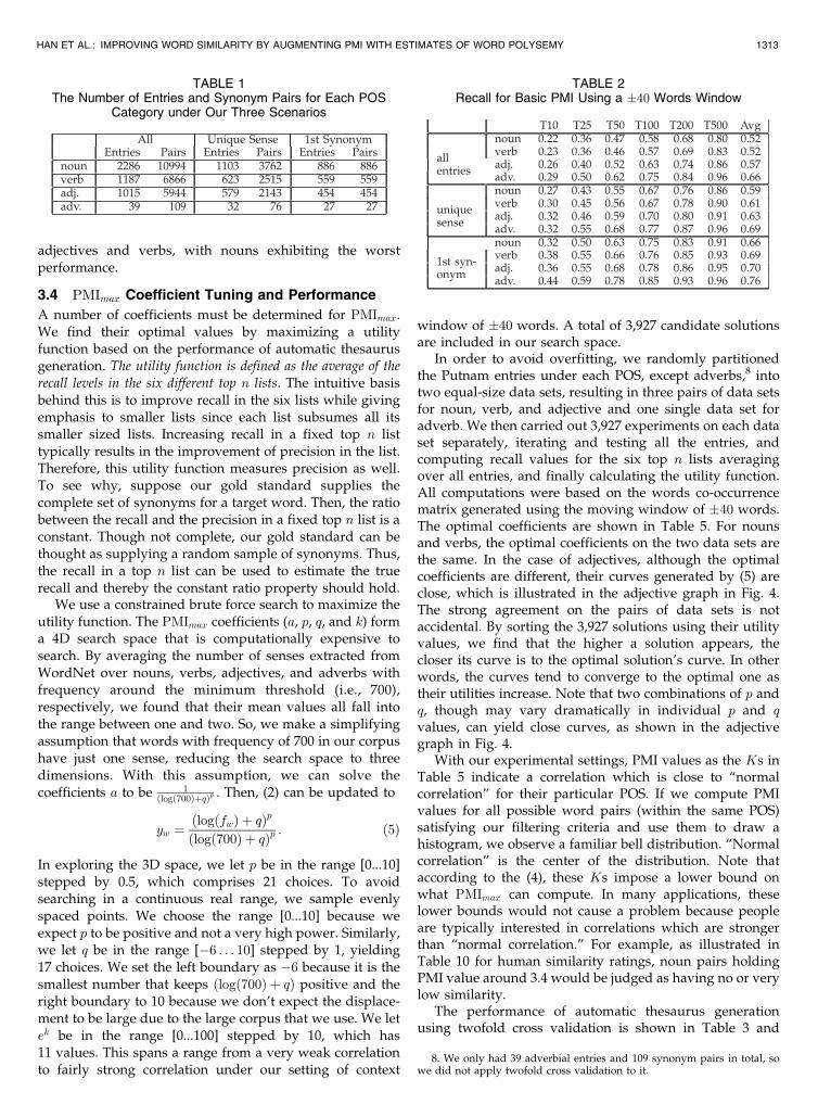
frequency less than 700 in the synonym lists of theremaining head words. In our experiment, we observedthat many synonyms have PMI values slightly above 7.0(see Table 10). Using the thresholds 10,000 and 700 enablesthem to co-occur at least four or five times, which istypically required to ensure PMI, a statistical approach,works reasonably [23]. In addition, multiwords terms andantonyms were removed.

Words can have multiple senses and many synonyms arenot completely synonymous but overlap in particularsenses. We would like to evaluate PMI’s performance infinding synonyms with different degrees of overlap. Toenable this kind of evaluation, we tested using threescenarios: 1) all entries; 2) entries with a unique sense;and 3) entries with a unique sense and only using the firstsynonym.6 Our rationale is that the single sense wordsshould have a greater semantic overlap with their syno-nyms and moreover the largest semantic overlap with theirfirst synonyms. Although we require the head words tohave a unique sense, their synonyms may still be poly-semous. Table 1 shows the number of entries and synonympairs in three scenarios with different part of speech tags.

3.3 Performance of Basic PMI

In our basic PMI algorithm, word co-occurrences7 arecounted in a moving window of a fixed size that scansthe entire corpus. To select the optimal window size for the

basic PMI metric, we experimented with 14 sizes, starting at�5 and ending at �70 with a step of five words. Windowswere not allowed to cross a paragraph boundary and weused a stopword list consisting of only the three articles “a,”“an,” and “the.”

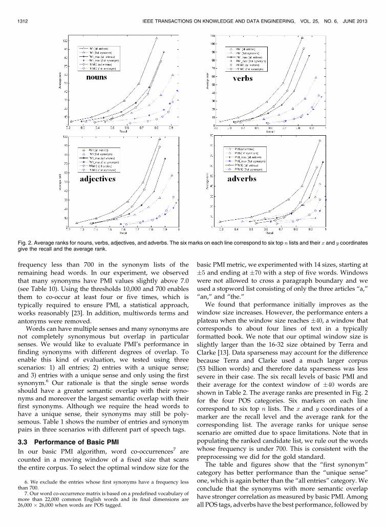
We found that performance initially improves as thewindow size increases. However, the performance enters aplateau when the window size reaches �40, a window thatcorresponds to about four lines of text in a typicallyformatted book. We note that our optimal window size isslightly larger than the 16-32 size obtained by Terra andClarke [13]. Data sparseness may account for the differencebecause Terra and Clarke used a much larger corpus(53 billion words) and therefore data sparseness was lesssevere in their case. The six recall levels of basic PMI andtheir average for the context window of �40 words areshown in Table 2. The average ranks are presented in Fig. 2for the four POS categories. Six markers on each linecorrespond to six top n lists. The x and y coordinates of amarker are the recall level and the average rank for thecorresponding list. The average ranks for unique sensescenario are omitted due to space limitations. Note that inpopulating the ranked candidate list, we rule out the wordswhose frequency is under 700. This is consistent with thepreprocessing we did for the gold standard.

The table and figures show that the “first synonym”category has better performance than the “unique sense”one, which is again better than the “all entries” category. Weconclude that the synonyms with more semantic overlaphave stronger correlation as measured by basic PMI. Amongall POS tags, adverbs have the best performance, followed by


Fig. 2. Average ranks for nouns, verbs, adjectives, and adverbs. The six marks on each line correspond to six top n lists and their x and y coordinatesgive the recall and the average rank.

6. We exclude the entries whose first synonyms have a frequency lessthan 700.

7. Our word co-occurrence matrix is based on a predefined vocabulary ofmore than 22,000 common English words and its final dimensions are26,000 � 26,000 when words are POS tagged.

adjectives and verbs, with nouns exhibiting the worstperformance.

3.4 PMImax Coefficient Tuning and Performance

A number of coefficients must be determined for PMImax.We find their optimal values by maximizing a utilityfunction based on the performance of automatic thesaurusgeneration. The utility function is defined as the average of therecall levels in the six different top n lists. The intuitive basisbehind this is to improve recall in the six lists while givingemphasis to smaller lists since each list subsumes all itssmaller sized lists. Increasing recall in a fixed top n listtypically results in the improvement of precision in the list.Therefore, this utility function measures precision as well.To see why, suppose our gold standard supplies thecomplete set of synonyms for a target word. Then, the ratiobetween the recall and the precision in a fixed top n list is aconstant. Though not complete, our gold standard can bethought as supplying a random sample of synonyms. Thus,the recall in a top n list can be used to estimate the truerecall and thereby the constant ratio property should hold.

We use a constrained brute force search to maximize theutility function. The PMImax coefficients (a, p, q, and k) forma 4D search space that is computationally expensive tosearch. By averaging the number of senses extracted fromWordNet over nouns, verbs, adjectives, and adverbs withfrequency around the minimum threshold (i.e., 700),respectively, we found that their mean values all fall intothe range between one and two. So, we make a simplifyingassumption that words with frequency of 700 in our corpushave just one sense, reducing the search space to threedimensions. With this assumption, we can solve thecoefficients a to be 1

ðlogð700ÞþqÞp . Then, (2) can be updated to

yw ¼ðlogðfwÞ þ qÞp

ðlogð700Þ þ qÞp : ð5Þ

In exploring the 3D space, we let p be in the range [0...10]stepped by 0.5, which comprises 21 choices. To avoidsearching in a continuous real range, we sample evenlyspaced points. We choose the range [0...10] because weexpect p to be positive and not a very high power. Similarly,we let q be in the range [�6 . . . 10] stepped by 1, yielding17 choices. We set the left boundary as �6 because it is thesmallest number that keeps ðlogð700Þ þ qÞ positive and theright boundary to 10 because we don’t expect the displace-ment to be large due to the large corpus that we use. We letek be in the range [0...100] stepped by 10, which has11 values. This spans a range from a very weak correlationto fairly strong correlation under our setting of context

window of �40 words. A total of 3,927 candidate solutionsare included in our search space.

In order to avoid overfitting, we randomly partitionedthe Putnam entries under each POS, except adverbs,8 intotwo equal-size data sets, resulting in three pairs of data setsfor noun, verb, and adjective and one single data set foradverb. We then carried out 3,927 experiments on each dataset separately, iterating and testing all the entries, andcomputing recall values for the six top n lists averagingover all entries, and finally calculating the utility function.All computations were based on the words co-occurrencematrix generated using the moving window of �40 words.The optimal coefficients are shown in Table 5. For nounsand verbs, the optimal coefficients on the two data sets arethe same. In the case of adjectives, although the optimalcoefficients are different, their curves generated by (5) areclose, which is illustrated in the adjective graph in Fig. 4.The strong agreement on the pairs of data sets is notaccidental. By sorting the 3,927 solutions using their utilityvalues, we find that the higher a solution appears, thecloser its curve is to the optimal solution’s curve. In otherwords, the curves tend to converge to the optimal one astheir utilities increase. Note that two combinations of p andq, though may vary dramatically in individual p and qvalues, can yield close curves, as shown in the adjectivegraph in Fig. 4.

With our experimental settings, PMI values as the Ks inTable 5 indicate a correlation which is close to “normalcorrelation” for their particular POS. If we compute PMIvalues for all possible word pairs (within the same POS)satisfying our filtering criteria and use them to draw ahistogram, we observe a familiar bell distribution. “Normalcorrelation” is the center of the distribution. Note thataccording to the (4), these Ks impose a lower bound onwhat PMImax can compute. In many applications, theselower bounds would not cause a problem because peopleare typically interested in correlations which are strongerthan “normal correlation.” For example, as illustrated inTable 10 for human similarity ratings, noun pairs holdingPMI value around 3.4 would be judged as having no or verylow similarity.

The performance of automatic thesaurus generationusing twofold cross validation is shown in Table 3 and


TABLE 2Recall for Basic PMI Using a �40 Words Window

TABLE 1The Number of Entries and Synonym Pairs for Each POS

Category under Our Three Scenarios

8. We only had 39 adverbial entries and 109 synonym pairs in total, sowe did not apply twofold cross validation to it.

Fig. 2. Although the coefficients are learned from the “allentries” scenario, the same coefficients are applied togenerate the results for the “unique sense” and “firstsynonym” scenarios. As Table 3 shows, the recall valuesenjoy significant improvements over basic PMI for all of thescenarios, POS tags, and top n lists. Some recall values, forexample, verbs in top 10 list as “first synonym,” received a50 percent increase. The improvements on all the recallvalues are statistically significant (p < 0:001 two-tailedpaired t-test). Regarding average rank, the comparisonshould be based on the same recall level instead of the sametop n list. This is because a list with larger recall maycontain more synonyms with bigger ranks and thereforedraw down the average rank. Fig. 2 clearly shows that, atthe same recall level, average ranks for PMImax get across-the-board improvements upon basic PMI.

Compare PMImax’s top 50 candidates for the verb“quicken” to those shown for PMI in Section 3.2.

slacken, stimulate, invigorate, regenerate, throb, accelerate,intensify, exhilarate, kindle, deepen, deaden, sharpen,retard, enliven, near, awaken, revive, thrill, heighten, over-take, pulse, broaden, stir, lag, sicken, infuse, expand, slow,brighten, dilate, strengthen, dull, purify, refresh, hasten,begrudge, spur, trot, career, nerve, freshen, hurry, blunt,sanctify, warm, cluck, inspire, lengthen, speed, impart

For this example, four synonyms for the word “quick-en” appear in the top 50 candidate list and are marked asbold. Their ranks are 2, 6, 17, and 35, so the recall valuesfor top 10, 25, and 50 lists are 2/12, 3/12, and 4/12,respectively. The average ranks for top 10, 25, and 50 listsare 4, 8.3, and 15. These numbers all improve upon thenumbers using basic PMI. High frequency verbs like“spur,” “hurry,” and “speed,” which are not shown bybasic PMI, also enter the ranking.

Fig. 3 shows additional examples of synonym listsproduced by PMI and PMImax, displaying a word and itstop 50 most similar words for each syntactic category.Words presented in both lists are marked as italic. Theexamples show that synonyms are generally ranked at thetop places by both methods. However, antonyms can haverankings as high as synonyms because antonyms (e.g.,“twist” and “straighten”) have many contexts in commonand a single negation may reverse their meaning to oneanother. Among all POS examples, the noun “car” exhibitsthe worse performance. Nevertheless, synonyms andsimilar concepts for “car,” such as “automobile,” “limou-sine,” and “truck” still show up in the top 50 lists of both

PMI and PMImax. The very top places of “chauffeur,”“garage,” and “headlight” suggest that both measureshighly rank a special kind of relation: nouns that areformed specifically for use in relation to the target noun. Inthe definitions of these nouns, the target noun is typicallyused. For example, “chauffeur” is defined in WordNet as “aman paid to drive a privately owned car.” The advantage ofthese nouns in computing PMI similarity comes from thefact that they seldom have their own contexts which are notsubsumed by the contexts of the target noun. PMI similarityis context based, which means that the similarity is notsolely relied on “IS-A” relation but an overall effect of allkinds of relations embodied by the contexts in a corpus.


TABLE 3Recall for PMImax Using �40 Words Window

Fig. 3. Four pairs of examples, showing the top 50 most similar words byPMI and PMI_max.

The examples show that PMI and PMImax capture almost

the same kind of semantic relations and many of the words in

their top 50 lists are the same. Their key difference is how

they rank low-frequency and high-frequency words. PMI is

predisposed toward low-frequency words and PMImaxalleviates this bias. For example, the topmost candidates

for “twist,” “ridiculous,” and “commonly” produced by PMI

are “contort,” “nonsensical,” and “supposedly,” respec-

tively, which are less common than the corresponding words

generated by PMImax, “writhe”, “absurd,” and “generally,”

although they have close meanings. The overall adjustment

made by PMImax is that low-frequency words move down

the list and high-frequency words move up with the

constraint that more similar words are still ranked higher.

Low-frequency words at the top of the PMI list are often good

synonyms. Though moved down, they typically remain in

the PMImax list. Low-frequency words which are more lowly

ranked tend to be not very similar to the target; in the PMImaxlist, they are replaced with higher frequency words.

In the example of “twist,” high-frequency words (e.g.,

“round,” “wind,” “spin,” “fasten,” “jerk,” “weave,” “curve,”

“double” and “bend”) move in the list to replace low-

frequency words including noisy words (e.g., “blotch” and

“lacquer”), less similar words (e.g., “groove” and “lunge”),

and less commonly used similar words (e.g., “flex” and

“crochet”). In the example of “car,” two important similar

words “vehicle” and “wheel” appear in the PMImax list after

the adjustment.Because PMImax estimates semantic similarity between

the closest senses of two words, it has an advantage over

PMI in discovering polysemous synonyms or similar

words. As examples, “double” has a sense of bend and

PMImax find it similar to “twist”; “platform” can mean

vehicle carrying weapons and PMImax find it similar to

“car”; “pathetic” has a sense of inspiring scornful pity and

PMImax find it similar to “ridiculous”.The frequency counts of the verb “double,” noun

“platform,” and adjective “pathetic” in our Gutenbergcorpus are 32,385, 60,114, and 28,202 and their assumedsenses (according to (5) and Table 5) are 6.5, 4.5, and 6.0,respectively. They are ranked at 106th, 64th, and 108thplaces in their PMI lists. They are able to move up in thePMImax lists because they have more assumed senses thanmany words in the PMI lists. Here, we zoom in on aconcrete example that compares a moving-out word“blotch” to a moving-in word “double.” “Blotch” has afrequency count 1,149 and co-occurs with “twist” 18 times,producing a PMI value 6.35. “Double” has a lower PMIvalue, 5.98, and co-occurs with “twist” 349 times. However,since “blotch” only has 1.5 assumed senses its PMImax valueis 8.71, which is smaller than the PMImax value between“double” and “twist,” 9.75.

The PMImax list for the adverb “commonly” has some

words that are often seen in a stopwords list, such as

“more,” “less,” “hence,” “also,” “either,” “very,” and

“however.” These words have very high frequencies but

few senses. PMImax erroneously judges them similar to

“commonly” because their high frequency mistakenly

suggests many senses.

3.5 Comparison to Distributional Similarity

To demonstrate the efficacy of PMImax in automaticthesaurus generation, we compare it with a state-of-the-artdistributional similarity measure proposed by Bullinariaand Levy [14]. Their method achieved the best performanceafter a series of work on distributional similarity from theirgroup [39], [40], [41]. The method is named Positive PMIcomponents and Cosine distances (PPMIC) because it usespositive pointwise mutual information to weight thecomponents in the context vectors and standard cosine tomeasure similarity between vectors. Bullinaria and Levydemonstrated that PPMIC was remarkably effective on arange of semantic and syntactic tasks, achieving, forexample, an accuracy of 85 percent on TOEFL synonymtest using the BNC corpus. Using PMI as the weightingfunction, and cosine as the similarity function is a popularchoice for measuring distributional similarity [30]. Whatmakes PPMIC different is a minimal context window size(�1 word window) and the use of a high-dimension contextvector that does not remove of low-frequency components.Bullinaria and Levy found that these uncommon settings areessential to make PPMIC work extremely well, though theyare not generally good choices for other similarity measures.

Our PPMIC implementation differs from Bullinaria andLevy’s in using lemmatized and POS-tagged words (noun,verb, adjectives, and adverbs) rather than unprocessedwords as vector dimension. This variation is simply due toconvenience of reusing what we already have. We testedour implementation of PPMIC on TOEFL synonym test andobtained a score of 80 percent. The slightly lowerperformance may result from the variation we made orthe use of the outdated Gutenberg corpus to answerquestions about modern English. Nevertheless, 80 percentis a very good score on TOEFL synonym test. As anexample, Bullinaria and Levy’s previous best result, beforeinventing PPMIC, was 75 percent [41].

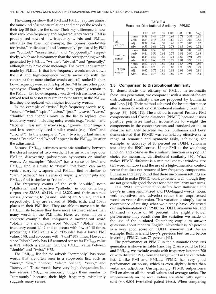
The performance of PPMIC in the automatic thesaurusgeneration is shown in Table 4 and Fig. 2. As we did for PMIand PMImax, we exclude words with frequency less than 700or with different POS from the target word in the candidatelist. Unlike PMI and PMImax, PPMIC has very goodperformance on nouns, which is even slightly better thanverbs and adjectives. Unsurprisingly, PPMIC outperformsPMI on almost all the recall values and average ranks. Theimprovements on the recall values are statistically signifi-cant (p < 0:001 two-tailed paired t-test). When comparing


TABLE 4Recall for Distributional Similarity—PPMIC

with PMImax, PPMIC has obvious advantage on nouns butjust competing performance on other POS categories.Although PPMIC leads PMImax on recall values for thesmall top n lists, such as top-10, PMImax can generally catchup quickly and outrun PPMIC for the subsequent longerlists. The same trend can also be observed on average ranksdepicted in Fig. 2. When considering all the recall values inTables 3 and 4, PMImax has a significantly better perfor-mance than PPMIC (p < 0:01 two-tailed paired t-test).Compared with PMImax, PPMIC seems to be able to rank aportion of synonyms very highly but it fails to give highscores to the remaining synonyms.

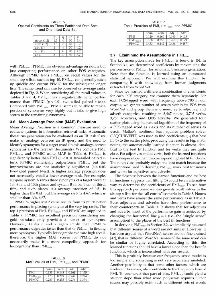
3.6 Mean Average Precision (MAP) Evaluation

Mean Average Precision is a common measure used toevaluate systems in information retrieval tasks. Automaticthesaurus generation can be evaluated as an IR task if wemake an analogy between an IR query and the need toidentify synonyms for a target word (in this analogy, correctsynonyms are the relevant documents). We compare PMI,PMImax, and PPMIC using MAP in Table 6. PMImax issignificantly better than PMI (p < 0:01 two-tailed paired t-test). PPMIC numerically outperforms PMImax but theimprovements are not statistically significant (p > 0:05two-tailed paired t-test). A higher average precision doesnot necessarily entail a lower average rank. For example,suppose system A ranks three synonyms of a target word at1st, 9th, and 10th places and system B ranks them at third,fifth, and sixth places. A’s average precision of 0.51 ishigher than B’s 0.41, but B’s average rank is 4.67, which issmaller than A’s, 6.67.

PPMIC’s higher MAP value results from its much betterperformance in placing synonyms at the very top ranks. Thetop-1 precision of PMI, PMImax, and PPMIC are supplied inTable 7. PPMIC has excellent precision, considering ourgold standard only provides a subset of synonyms.However, Tables 6 and 7 again imply that PPMIC’sperformance degrades faster than that of PMImax in findingmore synonyms. Typically lexicographers desire high recall,therefore, the higher MAP scores for PPMIC do notnecessarily make it a more compelling approach forlexicography than PMImax.

3.7 Examining the Assumptions in PMImaxThe key assumption made for PMImax is found in (5). InSection 3.4, we determined coefficients by maximizing theperformance of PMImax for automatic thesaurus generation.Note that the function is learned using an automatedstatistical approach. We will examine this function bycomparing it with knowledge from human judgmentsextracted from WordNet.

Since we learned a different combination of coefficientsfor each POS category, we examine them separately. Foreach POS-tagged word with frequency above 700 in ourcorpus, we get its number of senses within its POS fromWordNet and group them into noun, verb, adjective, andadverb categories, resulting in 8,467 nouns, 3,705 verbs,3,763 adjectives, and 1,095 adverbs. We generated fourscatter plots using the natural logarithm of the frequency ofa POS-tagged word as x-axis and its number of senses asy-axis. Matlab’s nonlinear least squares problem solver(LSQCURVEFIT) was used to find coefficients p, q that bestfit (5) to the scatter plots, producing the results in Fig. 4. Fornouns, the automatically learned function is almost iden-tical to the best fit function and for verbs they are quiteclose. For adjectives and adverbs, both the learned functionshave steeper slope than the corresponding best fit functions.The noun class probably enjoys the best match because theassumptions used in deriving PMImax work best for nounsand worst for adjectives and adverbs.

The closeness between the learned functions and the bestfit functions suggests that fitting (5) could be an alternativeway to determine the coefficients of PMImax. To see howthis approach performs, we also give its recall values in thesix top n lists for the “all entries” scenario in Table 8. Nounsand verbs have almost the same performance as in Table 3.Even adjectives and adverbs have close performance totheir counterparts in Table 3. It shows that for adjectivesand adverbs, most of the performance gain is achieved bychanging the horizontal line y ¼ 1 (i.e., the “single sense”assumption) to the places of the best fit functions.

In deriving PMImax in Section 2.2, we implicitly assumedthat different senses of a word are not similar. However, ithas been argued that WordNet’s senses are too fine grained[42], that is, different WordNet senses of the same word canbe similar or highly correlated. According to this, thelearned functions should have a lower slope than the best fitfunctions, which is inconsistent with our results.

This is probably because our frequency-sense model istoo simple and something is not very accurately modeled.Another possibility is that some other factors, which areirrelevant to senses, also contribute to the frequency bias ofPMI. To counteract that part of bias, PMImax could yield asteeper slope than what word polysemy requires. Othercauses may possibly exist, such as different sets of words


TABLE 5Optimal Coefficients on Three Partitioned Data Sets

and One Intact Data Set

TABLE 6MAP Values of PMI, PMImax, and PPMIC

TABLE 7Top-1 Precision of PMI, PMImax, and PPMIC

used in the automatic thesaurus generation experiment andin creating the plots, or missing senses in WordNet.

3.8 Low-Frequency Words Evaluation

We learned coefficients for PMImax using the occurrencefrequency thresholds 10,000 and 700 for target words andtheir synonyms. Now, we would like to check if PMImaxlearned in this way could produce consistently betterresults than PMI for low-frequency target words. To thisend, we extracted Putnam entries whose head words have afrequency between 700 and 2,000, obtaining 238, 103, and155 entries and 598, 282, and 449 synonym pairs for nouns,verbs, and adjectives, respectively. The recall values at sixtop n lists (“all entries” scenario) for PMI, PMImax, andPPMIC are shown in Table 9. Interestingly, PPMIC’sperformance for low-frequency words is even better thanits performance for high-frequency words, as compared toTable 4. More data typically lead to more accurate results instatistical approaches. PPMIC’s unusual result implies thatits performance is also affected by the degree of wordpolysemy. The case of low-frequency words is easier forPPMIC because they only have a few senses.

On the contrary, PMI and PMImax have degradedperformances compared to Tables 2 and 3 due to insufficient

data for them to work reasonably. In our experiment, the

expected co-occurrence between two strong synonyms (PMI

value 8.0) with the frequencies 700 and 1,000 is only 1. Thus,

many low-frequency synonyms lack even a single co-

occurrence with their targets while many noisy, low-

frequency words are ranked at top places by chance.

PMImax produces consistently better results than PMI

(p < 0:001 two-tailed paired t-test) but the improvement

rate is generally lowered, especially for large top n lists. We

see three reasons for this: some low-frequency synonyms

cannot be found regardless of the length of the ranked list

because they have no co-occurrences with the target, PMImaxranks noisy words downward but does not remove them in

the relatively long lists, and the coefficients are not

optimized for low-frequency target words.

4 BENCHMARK EVALUATION

In the preceding section, we demonstrated the effectiveness

of PMImax for automatic thesaurus generation. In this


Fig. 4. The frequency and the number of senses for nouns, verbs, adjectives, and adverbs.

TABLE 8Recall for PMImax Using Coefficients in Best Fit Functions

TABLE 9Recall for Low-Frequency Words

section, we will evaluate PMImax, tuned for the automaticthesaurus generation task, on common benchmark data setsincluding the Miller-Charles (MC) data set [46] and theTOEFL synonym test [25], allowing us to compare ourresults with previous systems. In these data sets, there arewords which occur less often in the Gutenberg corpus thanour frequency cutoff of 700. For these words, we assume asingle sense and apply (4) to compute PMImax.

4.1 Human Similarity Ratings

The widely used MC data set [8], [10], [9], [43], [22], [44],[45] consists of 30 pairs of nouns rated by a group of38 human subjects. Each subject rates “similarity of mean-ing” for each pair on a scale from 0 (no similarity) to4 (perfect synonymy). The mean of the individual ratingsfor each pair is used as its semantic similarity. The MC dataset was taken from Rubenstein-Goodenough’s (RG) [47]original data for 65 word pairs by selecting ten pairs ofhigh, intermediate, and low levels of similarity respectively.Although the MC experiment was performed 25 years afterRubenstein-Goodenough’s, the Pearson correlation coeffi-cient between the ratings is 0.97. Four years later, the sameexperiment was replicated again by Resnik [8] with10 subjects. Their mean ratings also had a very highcorrelation coefficient of 0.96. Resnik also showed that theindividual ratings in his experiment have an averagecorrelation coefficient 0.8848 with the MC mean ratings.

Due to the absence of the word “woodland” in earlierversions of WordNet, only 28 pairs are actually adopted bymost researchers. Our PMI implementation has a similarproblem in that “implement” has very low frequency (117)

in the Gutenberg corpus so that there are no co-occurrences

for “implement” and “crane.” Since their PMI value is

undefined, only 29 pairs can be used for our experiment.

For these, the correlation coefficient between the MC and

PMI ratings is 0.794, and for MC and PMImax is 0.852.

However, in order to compare with other people’s results, it

is necessary to have an equal setting. Fortunately, the

published papers of most previous researchers included

lists of ratings for each pair, allowing the comparison of our

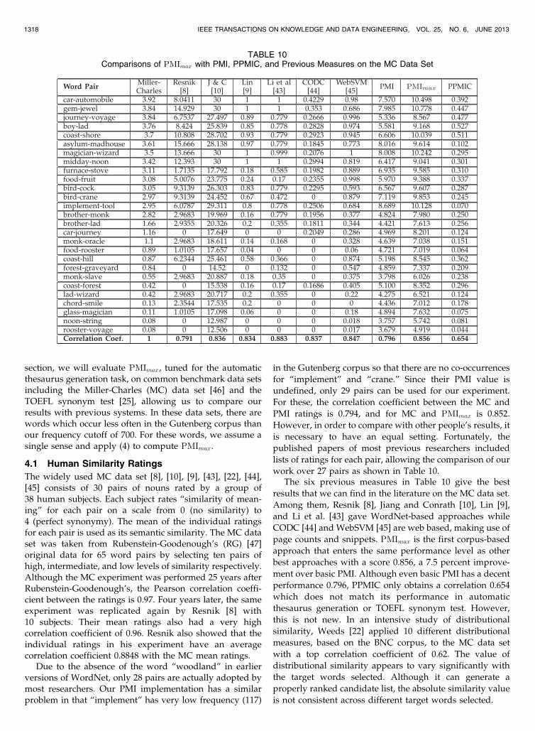
work over 27 pairs as shown in Table 10.The six previous measures in Table 10 give the best

results that we can find in the literature on the MC data set.

Among them, Resnik [8], Jiang and Conrath [10], Lin [9],

and Li et al. [43] gave WordNet-based approaches while

CODC [44] and WebSVM [45] are web based, making use of

page counts and snippets. PMImax is the first corpus-based

approach that enters the same performance level as other

best approaches with a score 0.856, a 7.5 percent improve-

ment over basic PMI. Although even basic PMI has a decent

performance 0.796, PPMIC only obtains a correlation 0.654

which does not match its performance in automatic

thesaurus generation or TOEFL synonym test. However,

this is not new. In an intensive study of distributional

similarity, Weeds [22] applied 10 different distributional

measures, based on the BNC corpus, to the MC data set

with a top correlation coefficient of 0.62. The value of

distributional similarity appears to vary significantly with

the target words selected. Although it can generate a

properly ranked candidate list, the absolute similarity value

is not consistent across different target words selected.


TABLE 10Comparisons of PMImax with PMI, PPMIC, and Previous Measures on the MC Data Set

We compare PMImax with basic PMI on two otherstandard data sets: Rubenstein-Goodenough [47] andWordSim353 [48]. Among 65 word pairs in the RG dataset, we removed five with undefined PMI and PMImaxvalues, and performed the experiment on the rest. Word-Sim353 contains 353 word pairs, each of which is scored by13 to 16 human subjects on a scale from 0 to 10. We removedproper nouns, such as “FBI” and “Arafat,” because they arenot supported by our current implementation of PMI andPMImax. We also imposed a minimum frequency thresholdof 200 to WordSim353 because it contains many modernwords such as “seafood” and “Internet” which occurinfrequently in our corpus. Choosing 200 as the thresholdis a compromise between keeping most of the word pairsavailable and making PMI and PMImax perform reliably.After all the preprocessing, 289 word pairs remains. Thecomparison results of PMI, PMImax, and PPMIC on the twodata sets along with the MC data set are shown in Table 11.Both the Pearson correlation and Spearman rank correlationcoefficients are investigated.

While PMImax’s Pearson correlation on the RG data set islower than its on the MC data set, its Spearman rankcorrelation on the RG data set is higher. WordSim353 is amore challenging data set than MC and RG. Our results,though lower than those on MC and RG, are still very good[48]. The improvements of PMImax over basic PMI usingeither Pearson correlation or Spearman rank correlation areall statistically significant (p < 0:05 with two-tailed paired t-test). Both PMI and PMImax have a consistently higherperformance than PPMIC on the three data sets.

4.2 TOEFL Synonym Questions

Eighty synonym questions were taken from the Test ofEnglish as a Foreign Language. Each is a multiple choicesynonym judgment, where the task is to select from fourcandidates the one having the closest meaning to thequestion word. Accuracy, which is the percentage ofcorrectly answered questions, is used to evaluate perfor-mance. The average score of foreign students applying toUS colleges from non-English speaking countries was64.5 percent [12].

This TOEFL synonym data set is widely used as abenchmark for comparing the performance of computa-tional similarity measures [12], [25], [41], [13], [49], [21], [14].Currently, the best results from corpus-based approachesare achieved by LSA [49], PPMIC [14], and PMI-IR [13],with scores of 92, 85, and 81.25 percent, respectively.

Since the words used in our implementations of PMI,PMImax, and PPMIC are POS tagged, we first assign a POStag to each TOEFL synonym question by choosing the

common POS of the question and candidate words. Theresults on the TOEFL synonym test for PMI, PMImax, andPPMIC are 72.5, 76.25, and 80 percent, respectively.Although the Gutenberg corpus has two billion words, itis still small compared with web collections used by PMI-IR. Thus, unlike PMI-IR, data sparseness is still a problemlimiting the performance of PMImax. For example, there arethree “no answer” questions9 for which the question wordhas no co-occurrence with any of four candidate words. It isknown that TOEFL synonym questions contain someinfrequently used words [14]. In addition, some TOEFLwords common in modern English, such as “highlight” and“outstanding,” were uncommon at the time of Gutenbergcorpus. A total of 76.25 percent is an encouraging resultbecause it demonstrates that PMImax need not rely onsearch engines to be effective in a difficult semantic task likethe TOEFL synonym questions.

5 DISCUSSION AND FUTURE WORK

PMImax can be used in various applications that requireword similarity measures. However, we are more interestedin combining PMImax with distributional similarity in thearea of semantic acquisition from text because this directionis not yet explored. We start our discussion by looking at anexample, the top 50 most similar words for the noun “car”generated by PPMIC.

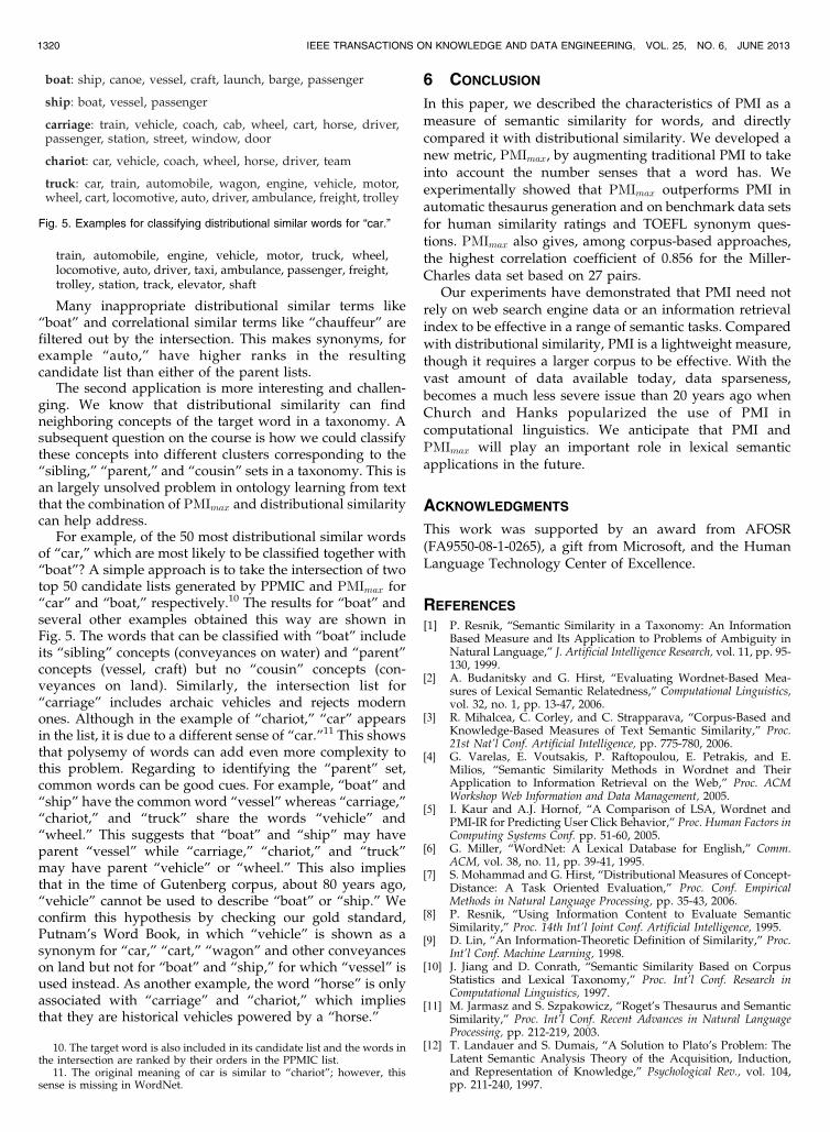
train, automobile, boat, wagon, carriage, engine, vehicle,motor, truck, coach, cab, wheel, ship, machine, cart,locomotive, chariot, canoe, vessel, craft, horse, bus, auto,driver, sleigh, gun, launch, taxi, buggy, barge, yacht,ambulance, passenger, freight, box, round, plane, trolley,station, team, street, track, window, rider, chair, mule,elevator, bicycle, door, shaft

The example shows that, as a state-of-the-art distribu-tional similarity, PPMIC has an amazing ability to find theconcepts that are functionality or utility similar to “car.”These concepts, such as “train,” “boat,” “carriage,” “vehi-cle,” are typically neighboring concepts of “car” in ataxonomy structure such as WordNet. In contrast, PMImax,as illustrated in the “car” example in Fig. 3, can only findsynonymous concepts and “siblings” concepts (e.g., “train”and “truck”) but miss the “cousin” concepts (e.g., “boat”and “carriage”). This is because PMI similarity measuresthe degree that two concepts tend to co-occur over theexactly same contexts. “Boat” and “carriage” are missingbecause only a small proportion of contexts of “car” relatesit to watercraft or archaic vehicles. Seemingly not aspowerful as distributional similarity, PMI similarity pro-vides a very useful complement to it.

There are many potential applications. Below, wesuggest two directions related to automatic thesaurus orontology generation. First, we could devise an improvedapproach for high-precision automatic thesaurus generationby taking intersection of the candidate lists generated byPMImax and a state-of-the-art distributional similarity, suchas PPMIC. For example, the intersection of two top-50candidate lists generated by PMImax and PPMIC for “car”includes:


TABLE 11Comparing PMImax with PMI on Three Data Sets

9. They are treated as incorrectly answered questions.

train, automobile, engine, vehicle, motor, truck, wheel,locomotive, auto, driver, taxi, ambulance, passenger, freight,trolley, station, track, elevator, shaft

Many inappropriate distributional similar terms like“boat” and correlational similar terms like “chauffeur” arefiltered out by the intersection. This makes synonyms, forexample “auto,” have higher ranks in the resultingcandidate list than either of the parent lists.

The second application is more interesting and challen-ging. We know that distributional similarity can findneighboring concepts of the target word in a taxonomy. Asubsequent question on the course is how we could classifythese concepts into different clusters corresponding to the“sibling,” “parent,” and “cousin” sets in a taxonomy. This isan largely unsolved problem in ontology learning from textthat the combination of PMImax and distributional similaritycan help address.

For example, of the 50 most distributional similar wordsof “car,” which are most likely to be classified together with“boat”? A simple approach is to take the intersection of twotop 50 candidate lists generated by PPMIC and PMImax for“car” and “boat,” respectively.10 The results for “boat” andseveral other examples obtained this way are shown inFig. 5. The words that can be classified with “boat” includeits “sibling” concepts (conveyances on water) and “parent”concepts (vessel, craft) but no “cousin” concepts (con-veyances on land). Similarly, the intersection list for“carriage” includes archaic vehicles and rejects modernones. Although in the example of “chariot,” “car” appearsin the list, it is due to a different sense of “car.”11 This showsthat polysemy of words can add even more complexity tothis problem. Regarding to identifying the “parent” set,common words can be good cues. For example, “boat” and“ship” have the common word “vessel” whereas “carriage,”“chariot,” and “truck” share the words “vehicle” and“wheel.” This suggests that “boat” and “ship” may haveparent “vessel” while “carriage,” “chariot,” and “truck”may have parent “vehicle” or “wheel.” This also impliesthat in the time of Gutenberg corpus, about 80 years ago,“vehicle” cannot be used to describe “boat” or “ship.” Weconfirm this hypothesis by checking our gold standard,Putnam’s Word Book, in which “vehicle” is shown as asynonym for “car,” “cart,” “wagon” and other conveyanceson land but not for “boat” and “ship,” for which “vessel” isused instead. As another example, the word “horse” is onlyassociated with “carriage” and “chariot,” which impliesthat they are historical vehicles powered by a “horse.”

6 CONCLUSION

In this paper, we described the characteristics of PMI as ameasure of semantic similarity for words, and directlycompared it with distributional similarity. We developed anew metric, PMImax, by augmenting traditional PMI to takeinto account the number senses that a word has. Weexperimentally showed that PMImax outperforms PMI inautomatic thesaurus generation and on benchmark data setsfor human similarity ratings and TOEFL synonym ques-tions. PMImax also gives, among corpus-based approaches,the highest correlation coefficient of 0.856 for the Miller-Charles data set based on 27 pairs.

Our experiments have demonstrated that PMI need notrely on web search engine data or an information retrievalindex to be effective in a range of semantic tasks. Comparedwith distributional similarity, PMI is a lightweight measure,though it requires a larger corpus to be effective. With thevast amount of data available today, data sparseness,becomes a much less severe issue than 20 years ago whenChurch and Hanks popularized the use of PMI incomputational linguistics. We anticipate that PMI andPMImax will play an important role in lexical semanticapplications in the future.

ACKNOWLEDGMENTS

This work was supported by an award from AFOSR(FA9550-08-1-0265), a gift from Microsoft, and the HumanLanguage Technology Center of Excellence.

REFERENCES

[1] P. Resnik, “Semantic Similarity in a Taxonomy: An InformationBased Measure and Its Application to Problems of Ambiguity inNatural Language,” J. Artificial Intelligence Research, vol. 11, pp. 95-130, 1999.

[2] A. Budanitsky and G. Hirst, “Evaluating Wordnet-Based Mea-sures of Lexical Semantic Relatedness,” Computational Linguistics,vol. 32, no. 1, pp. 13-47, 2006.

[3] R. Mihalcea, C. Corley, and C. Strapparava, “Corpus-Based andKnowledge-Based Measures of Text Semantic Similarity,” Proc.21st Nat’l Conf. Artificial Intelligence, pp. 775-780, 2006.

[4] G. Varelas, E. Voutsakis, P. Raftopoulou, E. Petrakis, and E.Milios, “Semantic Similarity Methods in Wordnet and TheirApplication to Information Retrieval on the Web,” Proc. ACMWorkshop Web Information and Data Management, 2005.

[5] I. Kaur and A.J. Hornof, “A Comparison of LSA, Wordnet andPMI-IR for Predicting User Click Behavior,” Proc. Human Factors inComputing Systems Conf. pp. 51-60, 2005.

[6] G. Miller, “WordNet: A Lexical Database for English,” Comm.ACM, vol. 38, no. 11, pp. 39-41, 1995.

[7] S. Mohammad and G. Hirst, “Distributional Measures of Concept-Distance: A Task Oriented Evaluation,” Proc. Conf. EmpiricalMethods in Natural Language Processing, pp. 35-43, 2006.

[8] P. Resnik, “Using Information Content to Evaluate SemanticSimilarity,” Proc. 14th Int’l Joint Conf. Artificial Intelligence, 1995.

[9] D. Lin, “An Information-Theoretic Definition of Similarity,” Proc.Int’l Conf. Machine Learning, 1998.

[10] J. Jiang and D. Conrath, “Semantic Similarity Based on CorpusStatistics and Lexical Taxonomy,” Proc. Int’l Conf. Research inComputational Linguistics, 1997.

[11] M. Jarmasz and S. Szpakowicz, “Roget’s Thesaurus and SemanticSimilarity,” Proc. Int’l Conf. Recent Advances in Natural LanguageProcessing, pp. 212-219, 2003.

[12] T. Landauer and S. Dumais, “A Solution to Plato’s Problem: TheLatent Semantic Analysis Theory of the Acquisition, Induction,and Representation of Knowledge,” Psychological Rev., vol. 104,pp. 211-240, 1997.


Fig. 5. Examples for classifying distributional similar words for “car.”

10. The target word is also included in its candidate list and the words inthe intersection are ranked by their orders in the PPMIC list.

11. The original meaning of car is similar to “chariot”; however, thissense is missing in WordNet.

[13] E. Terra and C.L.A. Clarke, “Frequency Estimates for StatisticalWord Similarity Measures,” Proc. Human Language Technology andNorth Am. Chapter of the ACL Conf., pp. 244-251, 2003.

[14] J. Bullinaria and J. Levy, “Extracting Semantic Representationsfrom Word Cooccurrence Statistics: A Computational Study,”Behavior Research Methods, vol. 39, no. 3, pp. 510-526, 2007.

[15] D. Hindle, “Noun Classification from Predicate-Argument Struc-tures,” Proc. Ann. Meeting ACL, pp. 268-275, 1990.

[16] G. Grefenstette, Explorations in Automatic Thesaurus Discovery.Kluwer Academic Publishers, 1994.

[17] D. Lin, “Automatic Retrieval and Clustering of Similar Words,”Proc. 17th Int’l Conf. Computational Linguistics, pp. 768-774, 1998.

[18] J.R. Curran and M. Moens, “Improvements in AutomaticThesaurus Extraction,” Proc. Workshop Unsupervised Lexical Acqui-sition, pp. 59-66, 2002.

[19] D. Yang and D.M. Powers, “Automatic Thesaurus Construction,”Proc. 31st Australasian Conf. Computer Science, vol. 74, pp. 147-156,2008.

[20] Z. Harris, Mathematical Structures of Language. Wiley, 1968.[21] S. Pado and M. Lapata, “Dependency-Based Construction of

Semantic Space Models,” Computational Linguistics, vol. 33, no. 2,pp. 161-199, 2007.

[22] J.E. Weeds, “Measures and Applications of Lexical DistributionalSimilarity,” PhD dissertation, Univ. of Sussex, 2003.

[23] K. Church and P. Hanks, “Word Association Norms, MutualInformation and Lexicography,” Proc. 27th Ann. Conf. ACL, pp. 76-83, 1989.

[24] C. Manning and H. Schutze, Foundations of Statistical NaturalLanguage Processing. MIT Press, 1999.

[25] P. Turney, “Mining the Web for Synonyms: PMI-IR Versus LSA onTOEFL,” Proc. 12th European Conf. Machine Learning, pp. 491-502,2001.

[26] D. Higgins, “Which Statistics Reflect Semantics? RethinkingSynonymy and Word Similarity,” Proc. Int’l Conf. LinguisticEvidence, pp. 265-284, 2004.

[27] N. Kaji and M. Kitsuregawa, “Using Hidden Markov RandomFields to Combine Distributional and Pattern-Based WordClustering,” Proc. 22nd Int’l Conf. Computational Linguistics,pp. 401-408, 2008.

[28] W. Gale, K. Church, and D. Yarowsky, “One Sense Per Discourse,”Proc. DARPA Speech and Natural Language Workshop, pp. 233-237,1992.

[29] P. Turney, M. Littman, J. Bigham, and V. Shnayder, “CombiningIndependent Modules to Solve Multiple-Choice Synonym andAnalogy Problems,” Proc. Int’l Conf. Recent Advances in NaturalLanguage Processing (RANLP ’03), pp. 482-489, 2003.

[30] P. Pantel and D. Lin, “Discovering Word Senses from Text,” Proc.ACM SIGKDD Conf. Knowledge Discovery and Data Mining, pp. 613-619, 2002.

[31] J. Weeds and D. Weir, “Finding and Evaluating Sets of NearestNeighbours,” Proc. Second Int’l Conf. Corpus Linguistics, 2003.

[32] H. Wu and M. Zhou, “Synonymous Collocation Extraction UsingTranslation Information,” Proc. 41st Ann. Meeting Assoc. forComputational Linguistics, pp. 120-127, 2003.

[33] T. Dunning, “Accurate Methods for the Statistics of Surprise andCoincidence,” Computational Linguistics, vol. 19, no. 1, pp. 61-74,1993.

[34] M. Hart, “Project Gutenberg Electronic Books,” http://www.gutenberg.org/wiki/Main_Page, 1997.

[35] K. Toutanova, D. Klein, C. Manning, W. Morgan, A. Rafferty, andM. Galley, “Stanford Log-Linear Part-of-Speech Tagger,” http://nlp.stanford.edu/software/tagger.shtml, 2000.

[36] F. Smadja, “Retrieving Collocations from Text: Xtract,” Computa-tional Linguistics, vol. 19, no. 1, pp. 143-178, 1993.

[37] I. Dagan, S. Marcus, and S. Markovitch, “Contextual WordSimilarity and Estimation from Sparse Data,” Proc. Ann. MeetingAssoc. Computational Linguistics (ACL ’93), pp. 164-171, 1993.

[38] L.A. Flemming, “Putnam’s Word Book,” http://www.gutenberg.org/files/13188/13188-8.txt, 1913.

[39] M. Patel, J.A. Bullinaria, and J.P. Levy, “Extracting SemanticRepresentations from Large Text Corpora,” Proc. Fourth NeuralComputation and Psychology Workshop: Connectionist Representations,pp. 199-212, 1997.

[40] J.P. Levy, J.A. Bullinaria, and M. Patel, “Explorations in theDerivation of Semantic Representations from Word Co-occurrenceStatistics,” South Pacific J. Psychology, vol. 10, pp. 99-111, 1998.

[41] J.P. Levy and J.A. Bullinaria, “Learning Lexical Properties fromWord Usage Patterns: Which Context Words Should be Used?”Proc. Sixth Neural Computation and Psychology Workshop: Connec-tionist Models of Learning, Development and Evolution, pp. 273-282,2001.

[42] R. Navigli, “Meaningful Clustering of Senses Helps Boost WordSense Disambiguation Performance,” Proc. 21th Int’l Conf. Compu-tational Linguistics, pp. 105-112, 2006.

[43] Y. Li, Z. Bandar, and D. McLean, “An Approach for MeasuringSemantic Similarity between Words Using Multiple InformationSources,” IEEE Trans. Knowledge and Data Eng., vol. 15, no. 4,pp. 871-882, July/Aug. 2003.

[44] H. Chen, M. Lin, and Y. Wei, “Novel Association Measures UsingWeb Search with Double Checking,” Proc. Int’l Conf. ComputationalLinguistics and the 44th Ann. Meeting of the Assoc. for ComputationalLinguistics, pp. 1009-1016, 2006.

[45] D. Bollegala, Y. Matsuo, and M. Ishizuka, “Measuring SemanticSimilarity between Words Using Web Search Engines,” Proc. Int’lConf. World Wide Web (WWW), 2007.

[46] G. Miller and W. Charles, “Contextual Correlates of SemanticSimilarity,” Language and Cognitive Processes, vol. 6, no. 1, pp. 1-28,1991.

[47] H. Rubenstein and J. Goodenough, “Contextual Correlates ofSynonymy,” Comm. ACM , vol. 8, no. 10, pp. 627-633, 1965.

[48] L. Finkelstein, E. Gabrilovich, Y. Matias, E. Rivlin, Z. Solan, G.Wolfman, and E. Ruppin, “Placing Search in Context: The ConceptRevisited,” ACM Trans. Information Systems, vol. 20, no. 1, pp. 116-131, 2002.

[49] R. Rapp, “Word Sense Discovery Based on Sense DescriptorDissimilarity,” Proc. Ninth Machine Translation Summit, pp. 315-322, 2003.

Lushan Han received the BSc degree incomputer science from Beijing University. He iscurrently working toward the PhD degree incomputer science at the University of Maryland,Baltimore County (UMBC). His dissertationresearch is developing a novel high-level querysystem for linked Semantic Web data usingstatistical models of language and the linkeddata to interpret the query.

Tim Finin received degrees from MIT and theUniversity of Illinois and has also held positionsat the JHU Human Language TechnologyCenter of Excellence, Unisys, the University ofPennsylvania, and the MIT AI Laboratory. He isa professor of computer science at the Universityof Maryland, Baltimore County (UMBC). He hasmore than 30 years of experience in applicationsof artificial intelligence to problems in informationsystems and language understanding.

Paul McNamee is a principal research scientistwith the Johns Hopkins University AppliedPhysics Laboratory and the JHU Human Lan-guage Technology Center of Excellence. Hisresearch interests include multilingual informa-tion retrieval and technologies for automatedknowledge base population. His recent workinvolves identifying named-entities in text andlinking textual mentions to structured knowledgesources, such as Wikipedia.


Anupam Joshi received the BTech degree inelectrical engineering from IIT Delhi in 1989, andthe master’s and PhD degrees in computerscience from Purdue University in 1991 and1993, respectively. He is a professor of compu-ter science at the University of Maryland,Baltimore County (UMBC). He has held posi-tions in IBM Research, the University of Mis-souri, Columbia University, and PurdueUniversity. His research interests are in the

broad area of networked computing and intelligent systems.

Yelena Yesha received the BSc degree incomputer science from York University in 1984,and the MSc and PhD degrees in computer andinformation science from The Ohio State Uni-versity in 1986 and 1989, respectively. She is aprofessor of computer science at the Universityof Maryland, Baltimore County (UMBC). She isthe associate director of the US NationalScience Foundation (NSF) sponsored Centerfor Hybrid Multicore Productivity and Research

and the site director of UMBC’s Multicore Computational Center. She isa member of the IEEE Computer Society.

. For more information on this or any other computing topic,please visit our Digital Library at www.computer.org/publications/dlib.


Date post:	31-Jan-2017
Category:	Documents
Upload:	yelena
View:	212 times
Download:	0 times

Improving Word Similarity by Augmenting PMI with Estimates of Word Polysemy

Documents