in multi-dimensions Jonas Sukys 6HPLQDUIRU $SSOLHG :(4 ... · Jonas Sukys (SAM, ETH Zu rich) MLMC...

MLMC for systems of stochastic conservation lawsin multi-dimensions

Jonas Sukys

Seminar for Applied Mathematics (SAM),Department of Mathematics (D-MATH),

ETH Zurich, Switzerland.

MCQMC, UNSW, Sydney,February 15, 2012.

Joint work in progress with

I Siddhartha MishraI SAM, ETH Zurich, Switzerland

I Christoph SchwabI SAM, ETH Zurich, Switzerland

I Part of ETH interdisciplinary research grantI CH1-03 10-1

Jonas Sukys (SAM, ETH Zurich) MLMC for systems of stochastic conservation laws MCQMC, February 15, 2012 0 / 20

Hyperbolic nonlinearconservation laws

Nonlinear hyperbolic conservation laws

Conservation of the physical quantities (mass, momentum, energy):∂tU(x, t) + div F(U, x) = 0,

U(x, 0) = U0(x),x ∈ Rd , t > 0.

I Euler equations of compressible gas dynamics

I Magnetohydrodynamics (MHD) equations of plasma physics

I Shallow water equations

Numerical solution using Finite Volume Method (FVM):

I Cell averages:

Ui ≈1

∆x

∫ xi+ 1

2

xi− 1

2

U(x , t)dx

xixi+1/2xi-1/2xi-1

Ui

Ui-1Fi-1/2

Fi+1/2

I ODE: ∂tUi + (Fi+ 12− Fi− 1

2)/∆x = 0

I Approximate Riemann fluxes: HLL, Godunov (Roe)I Explicit time stepping: FE, SSP-RK2 with ∆t limited by CFL


Stochastic nonlinear SYSTEMS of balance laws

∂tU(x, t) + div F(U, x) = S(U, x), x ∈ Rd , t > 0. (1.1)

U(x, 0), F(·, x) and S(·, x) are uncertain −→ solution U(x, t) is also uncertain:∂

∂tU(x, t, ω) + div F(U, x, ω) = S(U, x, ω),

U(x, 0, ω) = U0(x, ω),∀ω ∈ Ω, (Ω,F ,P). (1.2)

NO well-posedness results for stochastic systems!

Assumption

Initial data, source and flux have finite point-wise mean and variance⇓

entropy solution exists and has finite mean and variance


Short review ofMC-FVM and MLMC-FVM

Monte Carlo FVM algorithm (MC-FVM)

We are interested in E[U(x, t)] and V[U(x, t)] with (x, t) - fixed.

1. Draw M i.i.d. samples of random quantities

Ui0(·),Fi (·),Si (·), i = 1, . . . ,M.

2. For each draw, solve for approximate (FVM) entropy solutions

Ui0(·),Fi (·),Si (·) −→ Ui (·, tn).

3. Estimate statistics of E[U(·, tn)] with:

EM [U(·, tn)] :=1

M

M∑i=1

Ui (·, tn).

Drawback: slow convergence + costly FVM −→ extremely expensive for d > 1.Jonas Sukys (SAM, ETH Zurich) MLMC for systems of stochastic conservation laws MCQMC, February 15, 2012 3 / 20

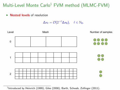
Multi-Level Monte Carlo1 FVM method (MLMC-FVM)

I Nested levels of resolution

∆x` = O(2−`∆x0), ` ∈ N0.

Level Number of samples

1

0

2

Mesh

1Introduced by Heinrich (1999); Giles (2008); Barth, Schwab, Zollinger (2011).

Multi-Level Monte Carlo FVM method (MLMC-FVM)

1. Draw M` i.i.d. samples of random quantities for each level `

Ui0,`(·),Fi

`(·),Si`(·), i = 1, . . . ,M.

2. For each draw i and level `, solve (with FVM)

Ui0,`(·),Fi

`(·),Si`(·) −→ Ui

`(·, tn).

3. Estimate statistics:

E[U(·, tn)] =∞∑`=0

E [U`(·, tn)−U`−1(·, tn)] , U−1 ≡ 0.

Fix L > 0 and estimate each term in the telescoping sum using MC-FVM

EL[U(·, tn)] =L∑

`=0

EM`[U`(·, tn)−U`−1(·, tn)].


Error vs. Work for Multi-Level Monte Carlo FVM

Theorem (Mishra & Schwab, 2010)

Denote FVM convergence rate by s > 0. For scalar CL with deterministic F,

‖E[U(tn)]− EL[U(tn)]‖L2(Ω;L1) ≤ C1∆x sL + C2

L∑

`=0

M− 1

2

` ∆x s`

+ C3M

− 12

0 ,

C1 = C1(U0, tn), C2 = C2(U0, tn), C3 = C3(U0).

Number of samples to equilibrate MC and FVM errors:

M` = O(22(L−`)s).

Cheap: error ∼ (Work)−s/(d+1) log(Work) if s < (d + 1)/2.


Euler equations: Cloud shock - initial dataUncertainty in shock location/magnitude and geometry of the cloud

0.0 0.2 0.4 0.6 0.8 1.00.0

0.2

0.4

0.6

0.8

1.0mean of rho at t=0.00

0.0

1.5

3.0

4.5

6.0

7.5

9.0

10.5

12.0

0.0 0.2 0.4 0.6 0.8 1.00.0

0.2

0.4

0.6

0.8

1.0variance of rho at t=0.00

0

5

10

15

20

25

30

35

40


Euler: MLMC-FVM for cloud shockwith uncertain shock location/magnitude and geometry of the cloud

0.0 0.2 0.4 0.6 0.8 1.00.0

0.2

0.4

0.6

0.8

1.0mean of rho at t=0.06

0

4

8

12

16

20

24

28

32

36

0.0 0.2 0.4 0.6 0.8 1.00.0

0.2

0.4

0.6

0.8

1.0log10(variance) of rho at t=0.06

2.0

1.5

1.0

0.5

0.0

0.5

1.0

1.5

2.0

2.5

L ML grid size CFL cores runtime efficiency9 8 4096x4096 0.4 1023 5:38:17 96.9%


MLMC algorithm is non-intrusive↓

Parallelization

Static load balancing for ALSVID-UQParallelization over levels, samples and subdomains

I Fix CL - number of cores for the finest level L,

I Use a-priori work estimates: ∀` < L, C` =

⌈C`+1

2d+1−2s

⌉.

Example setup:I L = 6, CL = 8,

I d = 1, s =1

2=⇒ C` =

C`+1

2.

level = 5 level = 4 level = 3

cores

samplers

# of samples

domaindecomposition

(ALSVID)

distributionof samples

1 1 1 1 2 2 2 2 8 8

?

2

32

1 & 0

64 & 128

multiple levelsper core


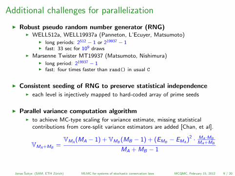
Additional challenges for parallelization

I Robust pseudo random number generator (RNG)I WELL512a, WELL19937a (Panneton, L’Ecuyer, Matsumoto)

I long periods: 2512 − 1 or 219937 − 1I fast: 33 sec for 109 draws

I Marsenne Twister MT19937 (Matsumoto, Nishimura)I long period: 219937 − 1I fast: four times faster than rand() in usual C

I Consistent seeding of RNG to preserve statistical independenceI each level is injectively mapped to hard-coded array of prime seeds

I Parallel variance computation algorithmI to achieve MC-type scaling for variance estimate, missing statistical

contributions from core-split variance estimators are added [Chan, et al].

VMA+MB=

VMA(MA − 1) + VMB

(MB − 1) + (EMB− EMA

)2 · MA·MB

MA+MB

MA + MB − 1


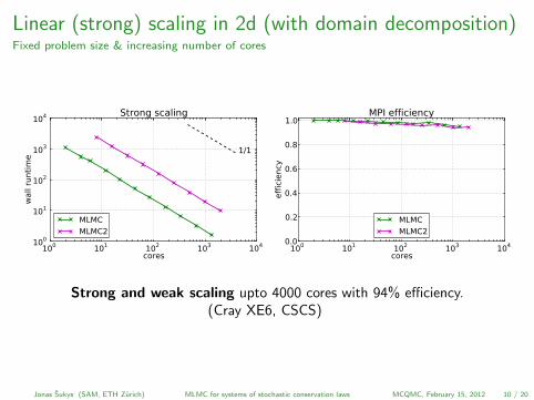
Linear (strong) scaling in 2d (with domain decomposition)Fixed problem size & increasing number of cores

100 101 102 103 104

cores

100

101

102

103

104

wall

runti

me

1/1

Strong scaling

MLMC

MLMC2

100 101 102 103 104

cores

0.0

0.2

0.4

0.6

0.8

1.0

eff

icie

ncy

MPI efficiency

MLMC

MLMC2

Strong and weak scaling upto 4000 cores with 94% efficiency.(Cray XE6, CSCS)


Convergence analysisfor numerical experiments

in 2D

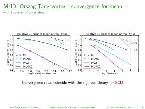
MHD: Orszag-Tang vortex - convergence for meanwith 2 sources of uncertainty

1.4 1.6 1.8 2.0 2.2 2.4 2.6 2.8log10(cells) in x-direction

0.0

0.2

0.4

0.6

0.8

1.0

1.2

1.4

log1

0( L

2(Ω,L

1)

err

or

) 1/2

1/1

Relative L1 error of mean of rho (K=5)

MC

MLMC

MC2

MLMC2

0 1 2 3 4 5 6 7log10(seconds)

0.0

0.2

0.4

0.6

0.8

1.0

1.2

1.4

log1

0( L

2(Ω,L

1)

err

or

)

1/6

1/3


MC

MLMC

MC2

MLMC2

Convergence rates coincide with the rigorous theory for SCL!


MHD: Orszag-Tang vortex - convergence for variancewith 2 sources of uncertainty


1.4

1.5

1.6

1.7

1.8

1.9

2.0

log1

0( L

2(Ω,L

1)

err

or

)

1/2

1/1

Relative L1 error of variance of rho (K=5)

MC

MLMC

MC2

MLMC2

0 1 2 3 4 5 6 7log10(seconds)

1.4

1.5

1.6

1.7

1.8

1.9

2.0

log1

0( L

2(Ω,L

1)

err

or

)

1/6

1/3


MC

MLMC

MC2

MLMC2


MHD: Orszag-Tang vortex - comparison of MLMC2for 2 and 8 sources of uncertainty


0.0

0.2

0.4

0.6

0.8

1.0

1.2

log1

0( L

2(Ω,L

1)

err

or

) 1/2

1/1


MLMC2 (2 sources)

MLMC2 (8 sources)

1.0 1.5 2.0 2.5 3.0 3.5 4.0 4.5 5.0log10(seconds)

0.0

0.2

0.4

0.6

0.8

1.0

1.2

log1

0( L

2(Ω,L

1)

err

or

) 1/6

1/3


MLMC2 (2 sources)

MLMC2 (8 sources)


Do we ever need more than10 or even 100 sources of uncertainty?

If yes, does MLMC-FVM still work?

Shallow water equations

Flows in rivers, lakes and oceans; atmospheric flows for weather prediction, etc.

U =

hhuhv

, F =

huhu2 + 1

2 gh2

huv

, G =

hvhuv

hv 2 + 12 gh2

, S =

0−ghbx(ω)−ghby (ω)

,

with bottom topography b ∈ L2(Ω,W 1,∞(D)).Ut + F(U)x + G(U)y = S(U, x , y , ω),

U(x , y , 0) = U0(x , y , ω).(x , y) ∈ D, t > 0, ∀ω ∈ Ω.


Uncertain bottom topography in 1dPiece-wise linear interpolation of uncertain topography measurements

xixi+1/2xi-3/2 xi-1/2xi-1

bi+1/2

bi-1/2

bi-3/2

bi+ 12(ω) := b(xi+ 1

2) + Yi (ω), Yi ∼ U(−εi , εi ), εi > 0,

bi+ 12(ω) ∈ L2(Ω,R) - random variables (not necessarily independent).


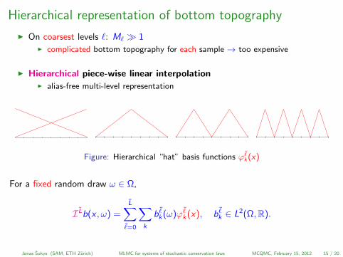
Hierarchical representation of bottom topography

I On coarsest levels `: M` 1I complicated bottom topography for each sample → too expensive

I Hierarchical piece-wise linear interpolationI alias-free multi-level representation

Figure: Hierarchical “hat” basis functions ϕ¯k(x)

For a fixed random draw ω ∈ Ω,

I Lb(x , ω) =L∑

¯=0

∑k

b¯k(ω)ϕ

¯k(x), b

¯k ∈ L2(Ω,R).


Truncated hierarchical representation

∆x ∆x

∆x ∆x

1 1/∆x

-1/∆x

ddx

Proposition (anti-aliasing)

AssumeL ≥ L ≥ `.

Then S`,Li with truncated I Lb coincides with S`,L

i with full I Lb, i.e.

S`,Li (ω) = S`,L

i (ω).

Minor modifications needed for:

I well-balanced staggered sources: L ≥ L ≥ ` + 1

I two-dimensional topographies: mixed tensor products (Schauder and Haar)

Bottom topography: one sample (realization)Hierarchical hat basis representation


Bottom topography: mean and standard deviationHierarchical hat basis representation


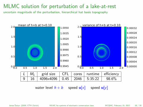
Shallow water: perturbation of a lake-at-restuncertain magnitude of the perturbation, hierarchical hat basis topography

0.0 0.5 1.0 1.5 2.00.0

0.5

1.0

1.5

2.0mean of h+b at t=0.00

1.0000

1.0025

1.0050

1.0075

1.0100

1.0125

1.0150

1.0175

1.0200

0.0 0.5 1.0 1.5 2.00.0

0.5

1.0

1.5

2.0variance of h+b at t=0.00

0.000000

0.000025

0.000050

0.000075

0.000100

0.000125

0.000150

0.000175

0.000200

0.000225


MLMC solution for perturbation of a lake-at-restuncertain magnitude of the perturbation, hierarchical hat basis topography

0.0 0.5 1.0 1.5 2.00.0

0.5

1.0

1.5

2.0mean of h+b at t=0.10

0.9945

0.9960

0.9975

0.9990

1.0005

1.0020

1.0035

1.0050

0.0 0.5 1.0 1.5 2.00.0

0.5

1.0

1.5

2.0variance of h+b at t=0.10

0.00000

0.00004

0.00008

0.00012

0.00016

0.00020

0.00024

0.00028

0.00032

L ML grid size CFL cores runtime efficiency9 16 4096x4096 0.45 2046 5:35:22 98.6%

water level h + b speed u[x ] speed u[y ]


Shallow water: Perturbation of a steady stateTruncated vs. full representation of uncertain botton topography

1.4 1.6 1.8 2.0 2.2 2.4 2.6log10(cells) in x-direction

0.45

0.40

0.35

0.30

0.25

0.20

0.15

0.10

0.05

0.00

log1

0( L

2(Ω,L

1)

err

or

)

1/2

1/1

Relative L1 error of mean of h+b (K=1)

MLMC2 full

MLMC2 truncated

1.0 1.5 2.0 2.5 3.0 3.5 4.0 4.5 5.0log10(seconds)

0.45

0.40

0.35

0.30

0.25

0.20

0.15

0.10

0.05

0.00

log1

0( L

2(Ω,L

1)

err

or

)

1/6

1/3

Relative L1 error of mean of h+b (K=1)

MLMC2 full

MLMC2 truncated

Full (L = 8) and truncated (` + 1) representation of bottom topography


Summary for MLMC-FVM methodI applicable to wide range of conservation laws

I Euler, MHD, shallow water, acoustic wave, linear elasticity

I 2 orders of magnitude speed-up of MLMC-FVM vs. MC-FVM

I computational complexity as in deterministic systems (asymptotically)

I flexible w.r.t. the origin of the uncertainty

I uncertain initial data, sources, fluxes, boundary conditions

I (at most) linear complexity of (ML)MC w.r.t. stochastic dimension

I gPC-based methods suffer from curse of dimensionality

I low regularity requirements

I non-intrusiveI deterministic FVM solvers can be reused

I easily parallelizable, highly scalableI strong (linear) and weak scaling in multi-dimensions

I work in progress:I free parameters - L and ML

I a-posteriori error estimate


Thank you.

References

I S. Mishra, Ch. Schwab and J. Sukys. Multi-level Monte Carlo finite volumemethods for nonlinear systems of conservation laws in multi-dimensions.J. Comp. Phys., 2011. DOI: 10.1016/j.jcp.2012.01.011

I S. Mishra, Ch. Schwab, and J. Sukys. Multi-level Monte Carlo Finite Volumemethods for shallow water equations with uncertain topography inmulti-dimensions. SISC, 2011 (submitted).

I J. Sukys, S. Mishra, and Ch. Schwab. Static load balancing for multi-levelMonte Carlo finite volume solvers. Parallel Processing and AppliedMathematics 9th International Conference, PPAM 2011, Torun, Poland, 2011(to appear).

I S. Mishra and Ch. Schwab. Sparse tensor multi-level Monte Carlo FiniteVolume Methods for hyperbolic conservation laws with random initial data.Math. Comp., 2011 (to appear).

I ALSVID-UQ. Available from http://mlmc.origo.ethz.ch/.

Available from: http://www.sam.math.ethz.ch/~sukysj

10.1016/j.jcp.2012.01.011

http://mlmc.origo.ethz.ch/

http://www.sam.math.ethz.ch/~sukysj

Error estimator 2

L2(Ω; L1(Rd))-based error estimator:

RE =

√√√√ K∑k=1

(REk)2/K , REk = 100× ‖Uref − Uk‖`1

‖Uref ‖`1

.

0 20 40 60 80 100 120 140 160 1802.1

2.2

2.3

2.4

2.5

2.6

2.7

2.8

2.9

3

Number of runs

Mean E

RR

OR

MC

MLMC

In 1d, based on above, we choose K = 30.In 2d, experience shows that K = 5 is sufficient.

2S. Mishra and Ch. Schwab, 2010.Jonas Sukys (SAM, ETH Zurich) MLMC for systems of stochastic conservation laws MCQMC, February 15, 2012 20 / 20

Behavior of MLMC error w.r.t. to parameter ML3

−2.5 −2 −1.5 −1 −0.5 0 0.5 1 1.5 2 2.50

0.1

0.2

0.3

0.4

0.5

0.6

0.7

0.8

0.9

1

log(runtime)

log(e

rror)

MC

MLMC (8)

MLMC (16)

MLMC(4)

Large problems and large number of levels?−→ smaller ML perform better.

3S. Mishra and Ch. Schwab, 2010.Jonas Sukys (SAM, ETH Zurich) MLMC for systems of stochastic conservation laws MCQMC, February 15, 2012 20 / 20

Optimality of the choices s = 1/2

1.5 2.0 2.5 3.0 3.5 4.0log10(cells) in x-direction

1.1

1.2

1.3

1.4

1.5

1.6

1.7

1.8

1.9

2.0

log1

0( L

2(Ω,L

1)

err

or

)

1/2

1/1


MC (s=1/2)

MC (s=1)

MLMC (s=1/2)

MLMC (s=1)

2 1 0 1 2 3 4log10(seconds)

1.1

1.2

1.3

1.4

1.5

1.6

1.7

1.8

1.9

2.0

log1

0( L

2(Ω,L

1)

err

or

)

1/4

1/2


MC (s=1/2)

MC (s=1)

MLMC (s=1/2)

MLMC (s=1)

s = 1 leads to much more work for th equivalent error level.


Sensitivity of MLMC to multiscale behavior in solution

0.0 0.5 1.0 1.5 2.01.5

1.0

0.5

0.0

0.5

1.0

1.5 mean of ux t=0.00

MC2

0.0 0.5 1.0 1.5 2.00.00000

0.00005

0.00010

0.00015

0.00020variance of ux t=0.00

MC2

OPTS: model: sod-shock-tube-multiscale, solver: hll3, multi: single, space: o2wenofVARS: NSAVES: 10, ML: 512, NX: 512INFO: nodes: 1, runtime: 0:01:02

Initial data with multiscale oscillationsthat are not resolved on 3 (out of 7) coarsest mesh levels!


Resolving multiscale oscillations - Burgers’

0.0 0.5 1.0 1.5 2.01.0

0.5

0.0

0.5

1.0mean of ux t=0.10

MC2MLMC2

0.0 0.5 1.0 1.5 2.00.00000

0.00002

0.00004

0.00006

0.00008

0.00010variance of ux t=0.10

MC2MLMC2

OPTS: model: sod-shock-tube-multiscale, solver: hll3, multi: single, space: o2wenofVARS: NX: 512, NSAVES: 10, ML: 16, L: 6INFO: nodes: 1, runtime: 0:00:36

Solution of Burgers’ equation using MC2 and MLMC2−→ both methods coincide!


Resolving multiscale oscillations - linear advection

0.0 0.5 1.0 1.5 2.00.4

0.6

0.8

1.0

1.2

1.4

1.6mean of Bx t=1.00

MC2MLMC2

0.0 0.5 1.0 1.5 2.00.00000

0.00002

0.00004

0.00006

0.00008

0.00010

0.00012variance of Bx t=1.00

MC2MLMC2

OPTS: model: magnetic-advection-multiscale, solver: hll3, multi: single, space: o2wenofVARS: NX: 512, NSAVES: 50, ML: 16, L: 6INFO: nodes: 1, runtime: 0:04:32

Solution of linear advection equation using MC2 and MLMC2−→ results are very different!


Date post:	01-Dec-2018
Category:	Documents
Upload:	docong
View:	213 times
Download:	0 times

in multi-dimensions Jonas Sukys 6HPLQDUIRU $SSOLHG :(4 ... · Jonas Sukys (SAM, ETH Zu rich) MLMC...

Documents