1

In-Place Associative Computing

Avidan Akerib Ph.D.

Vice President Associative Computing BU

aakerib@gsitechnology.com All Images are Public in the Web

2

Agenda

• Introduction to associative computing

• Use case examples

• Similarity search

• Large Scale Attention Computing

• Few-shot learning

• Software model

• Future Approaches

3

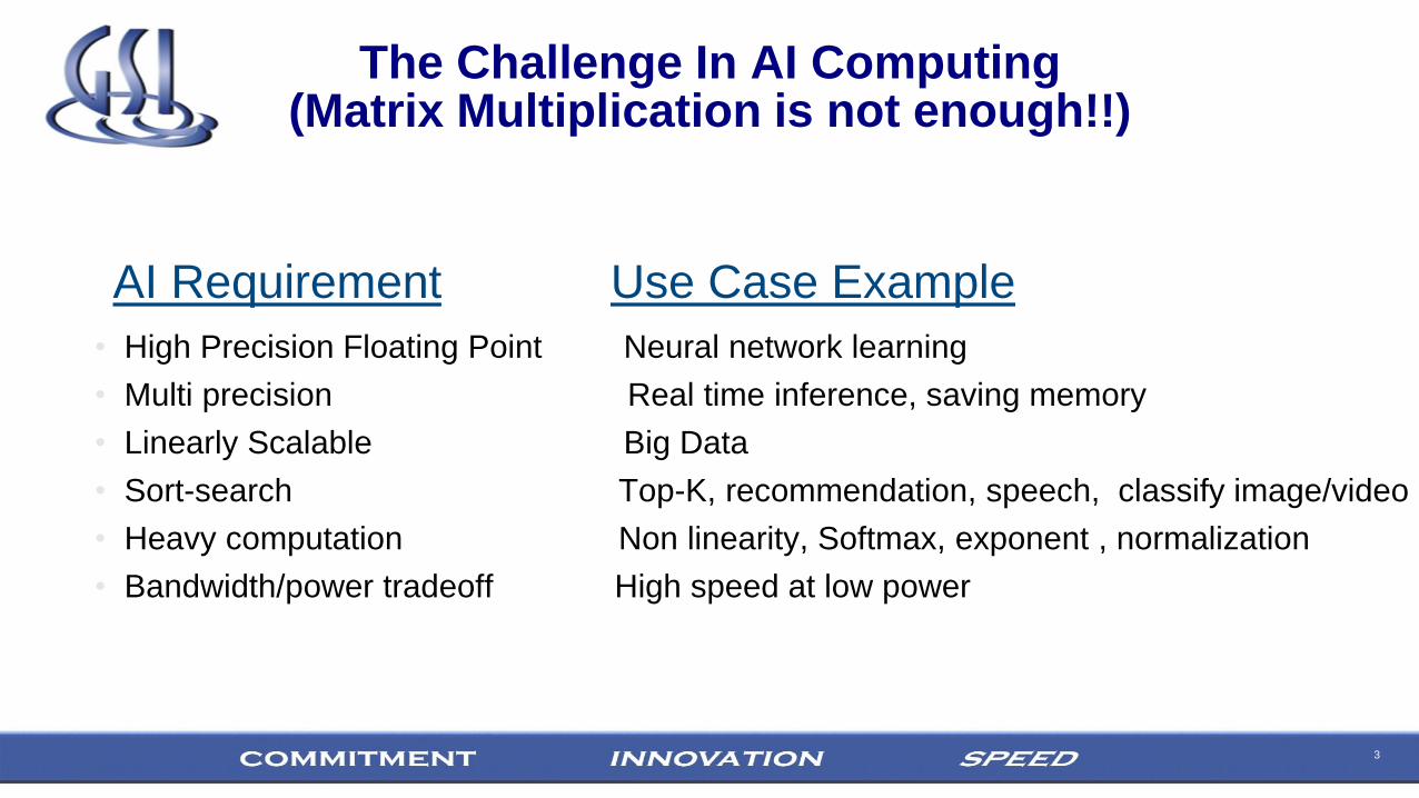
The Challenge In AI Computing(Matrix Multiplication is not enough!!)

AI Requirement

• High Precision Floating Point Neural network learning

• Multi precision Real time inference, saving memory

• Linearly Scalable Big Data

• Sort-search Top-K, recommendation, speech, classify image/video

• Heavy computation Non linearity, Softmax, exponent , normalization

• Bandwidth/power tradeoff High speed at low power

Use Case Example

4

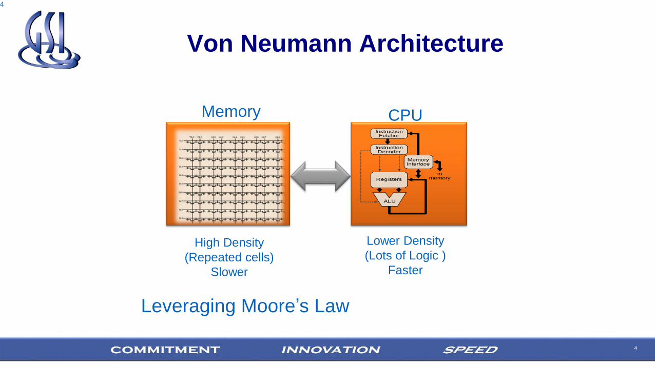
Von Neumann Architecture

4

CPUMemory

High Density

(Repeated cells)

Slower

Lower Density

(Lots of Logic )

Faster

Leveraging Moore’s Law

5

Von Neumann Architecture

5

CPUMemory

High Density

(Reputed cells)

Slower

Lower Density

(Lots of Logic)

Faster

CPU frequency outpacing memory - need to add

cache …. Continue to leverage Moore’s Law

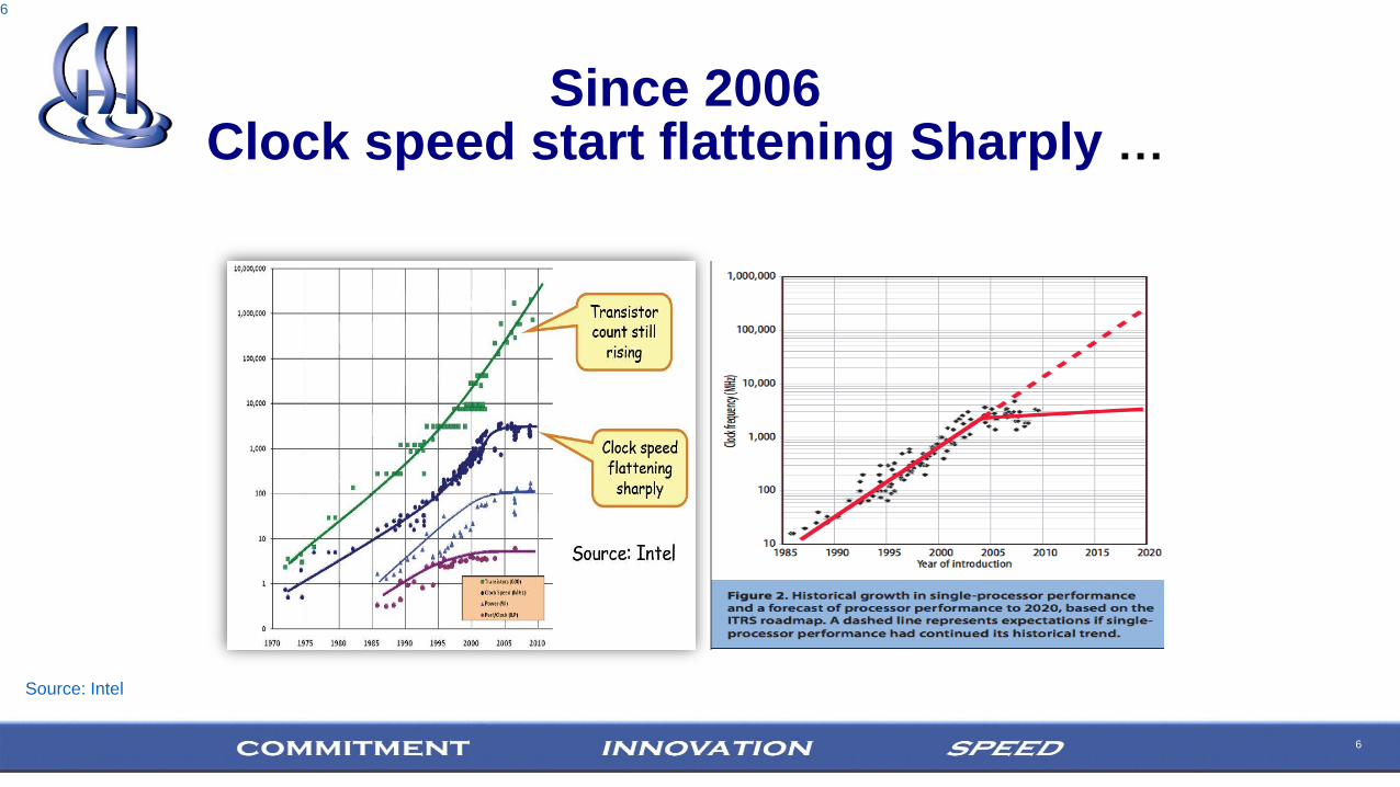
6

Since 2006 Clock speed start flattening Sharply …

6

Source: Intel

7

Thinking Parallel : 2 cores and more

7

CPUMemory

However, memory utilization becomes an issue …

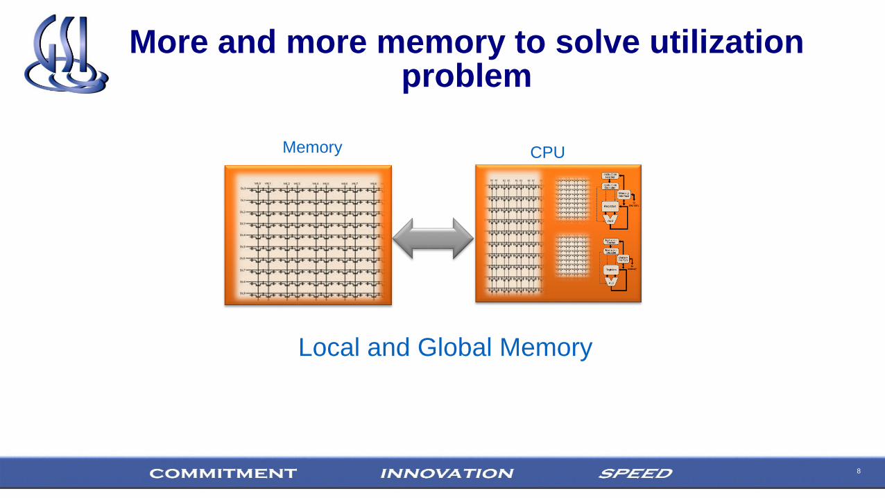
8

More and more memory to solve utilization problem

CPUMemory

Local and Global Memory

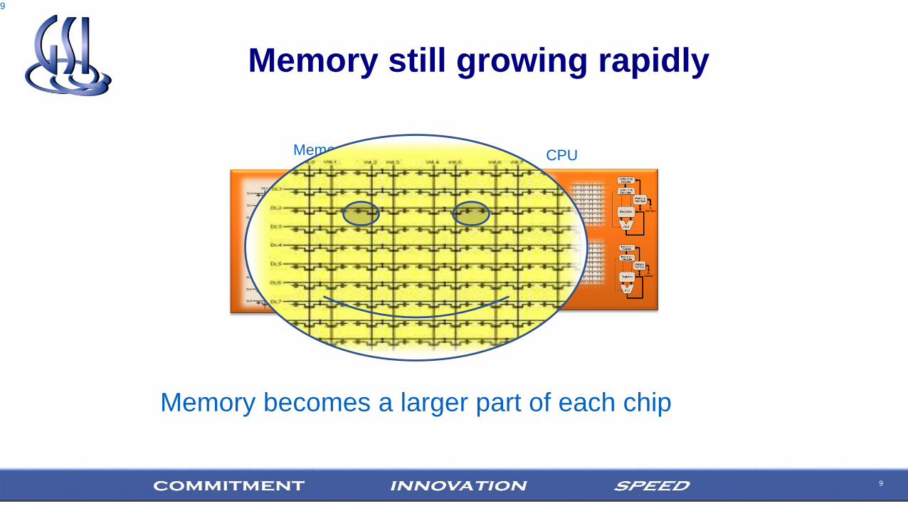
9

Memory still growing rapidly

9

CPUMemory

Memory becomes a larger part of each chip

10

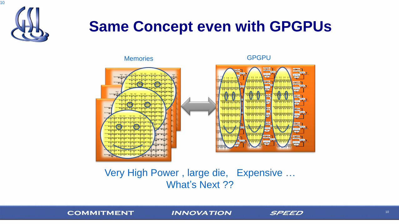
Same Concept even with GPGPUs

10

GPGPUMemories

Very High Power , large die, Expensive …

What’s Next ??

11

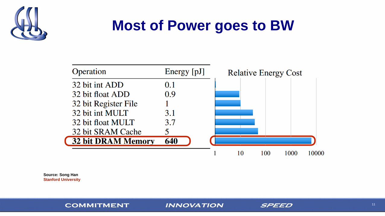
Most of Power goes to BW

Source: Song Han

Stanford University

12

Changing the Rules of the Game!!!

12

Standard Memory cells are smarter than we thought !!

13

APU—Associative Processing Unit

• Computes in-place directly in the memory array—removes the I/O

bottleneck

• Significantly increases performance

• Reduces power

Simple CPU

APU

Associative

Processing

Question

Answer

Simple

& Narrow Bus

Millions Processors

14

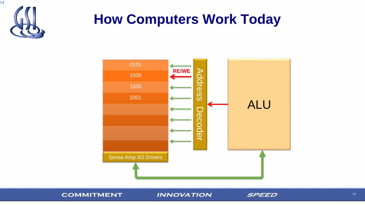
How Computers Work Today

14

1000

1100

1001

Addre

ss D

ecoder

Sense Amp /IO Drivers

ALU

0101

RE/WE

15

Accessing Multiple Rows Simultaneously

15

0101

1000

1100

1001

RE

RE

WE?0010NOR

0001

RE

RE

WE

Bus Contention is not an error !!!

It’s a simple NOR/NAND satisfying

De-Morgan’s law

16

Truth Table Example

A B C

0 0 0

0 0 1

0 1 0

0 1 1

1 0 0

1 0 1

1 1 0

1 1 1

D

1

0

1

1

0

0

0

1

AB

C00 01 11 10

1 1 0 0

0 1 1 0

0

1

!A!C + BC =

!!( !A!C + BC ) = ! (!(!A!C)!(BC))

= NAND( NAND(!A,!C),NAND(B,C))

Read (B,C) ; WRITE T2Read (!A,!C) ; WRITE T1

Read (T1,T2) ; WRITE D

1 CLOCK

1 CLOCK

• Every Minterm

takes one Clock

• All bit lines

executes Karnaugh

tables in parallel

17

Vector Add Example

17

A[] + B[] = C[]

No. Of Clocks = 4 * 8 = 32

Clocks/byte= 32/32M=1/1M

OPS = 1Ghz X 1M

= 1 PetaOPS

vector A(8,32M)

vector B(8,32M)

Vector C(9,32M)

C = A + B

18

1101

1000

1001

1

0

0

1

0

1

1

0

0010

0111

0110

Records

1=match00

Duplicate Vales with

inverse data

Duplicate the Key with

Inverse. Move The original

Key next to the inverse

data

RE

RE

RE

RE

1 in the combines

key goes to the

read enable

CAM/ Associative Search

ValuesKEY:

Search

0110

19

0

1

1

0

Don’t’ Care

010

Don’t Care

11

Don’t Care

0110

TCAM Search By Standard Memory Cells

20

0101

0000

1001

1

0

0

1

0

1

1

0

0010

0110

0110

KEY:

Search

0110

1=match01= match

Duplicate data. Inverse only to

those which are not don’t careDuplicate the Key with

Inverse. Move The

original Key next to the

inverse data

RE

RE

RE

RE

1 in the combines

key goes to the

read enable

Insert Zero instead of don’t-care

TCAM Search By Standard Memory Cells

21

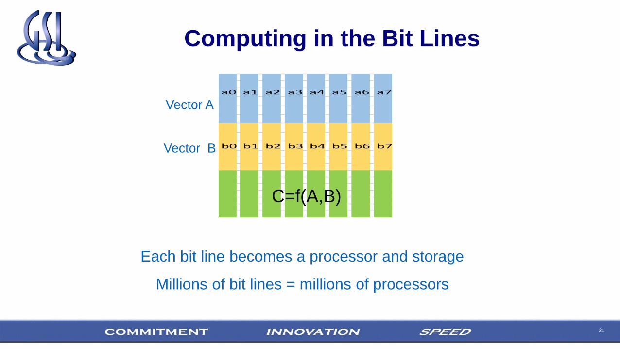
Computing in the Bit Lines

Vector A

Vector B

Each bit line becomes a processor and storage

Millions of bit lines = millions of processors

a0 a1 a2 a3 a4 a5 a6 a7

b0 b1 b2 b3 b4 b5 b6 b7

C=f(A,B)

22

Neighborhood Computing

Parallel shift of bit lines @ 1 cycle sections

Enables neighborhood operations such as convolutions

C=f(A,SL(B,1))

Shift vector

23

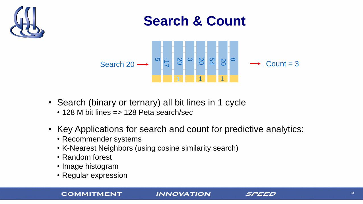
Search & Count

5

Count = 3 Search 20

20

-17

3 20

54

20

1 1 1

• Key Applications for search and count for predictive analytics:• Recommender systems

• K-Nearest Neighbors (using cosine similarity search)

• Random forest

• Image histogram

• Regular expression

8

• Search (binary or ternary) all bit lines in 1 cycle• 128 M bit lines => 128 Peta search/sec

1 1 1

24

CPU vs GPU vs FPGA vs APU

25

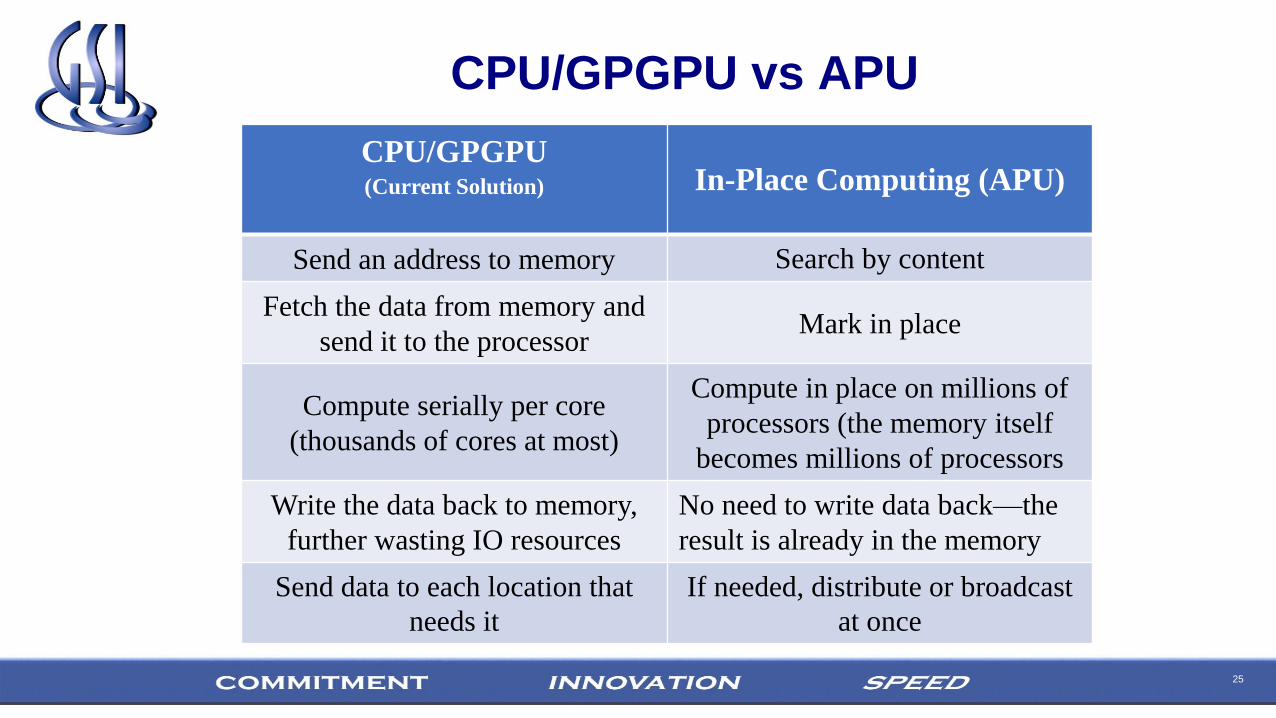
CPU/GPGPU vs APU

CPU/GPGPU(Current Solution) In-Place Computing (APU)

Send an address to memory Search by content

Fetch the data from memory and

send it to the processorMark in place

Compute serially per core

(thousands of cores at most)

Compute in place on millions of

processors (the memory itself

becomes millions of processors

Write the data back to memory,

further wasting IO resources

No need to write data back—the

result is already in the memory

Send data to each location that

needs it

If needed, distribute or broadcast

at once

26

ARCHITECTURE

27

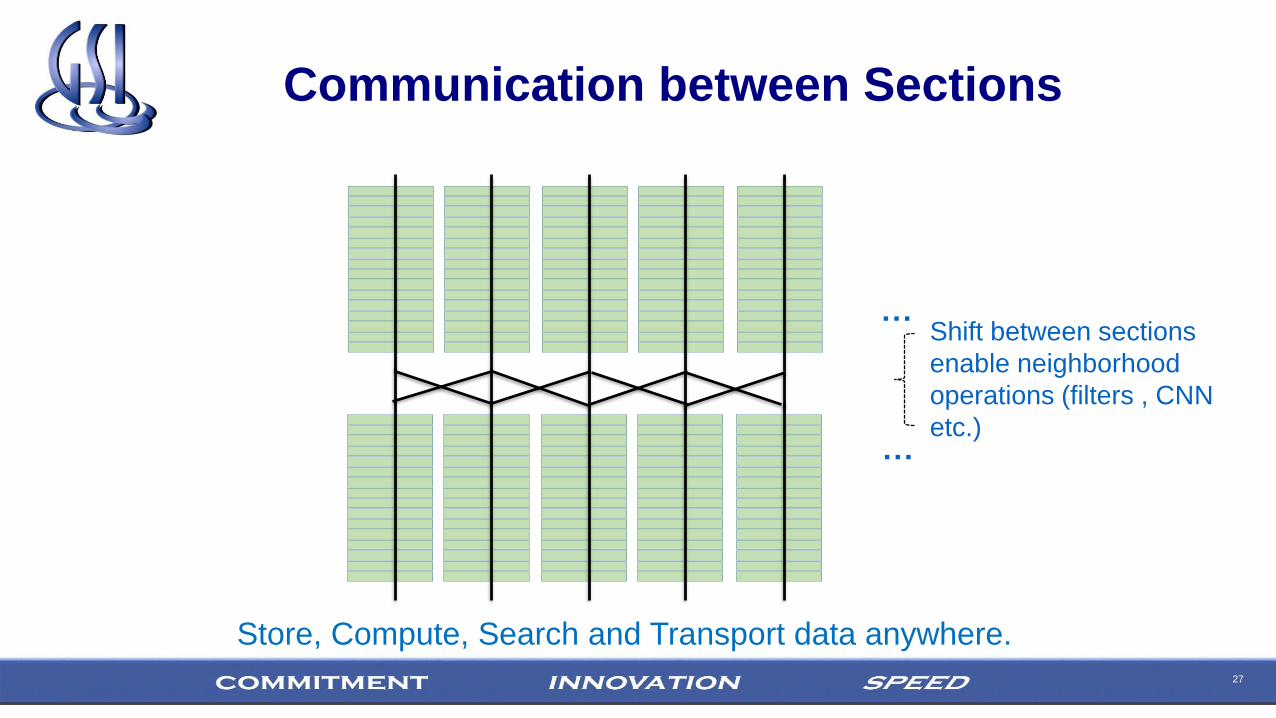
Store, Compute, Search and Transport data anywhere.

…

…

Shift between sections

enable neighborhood

operations (filters , CNN

etc.)

Communication between Sections

28

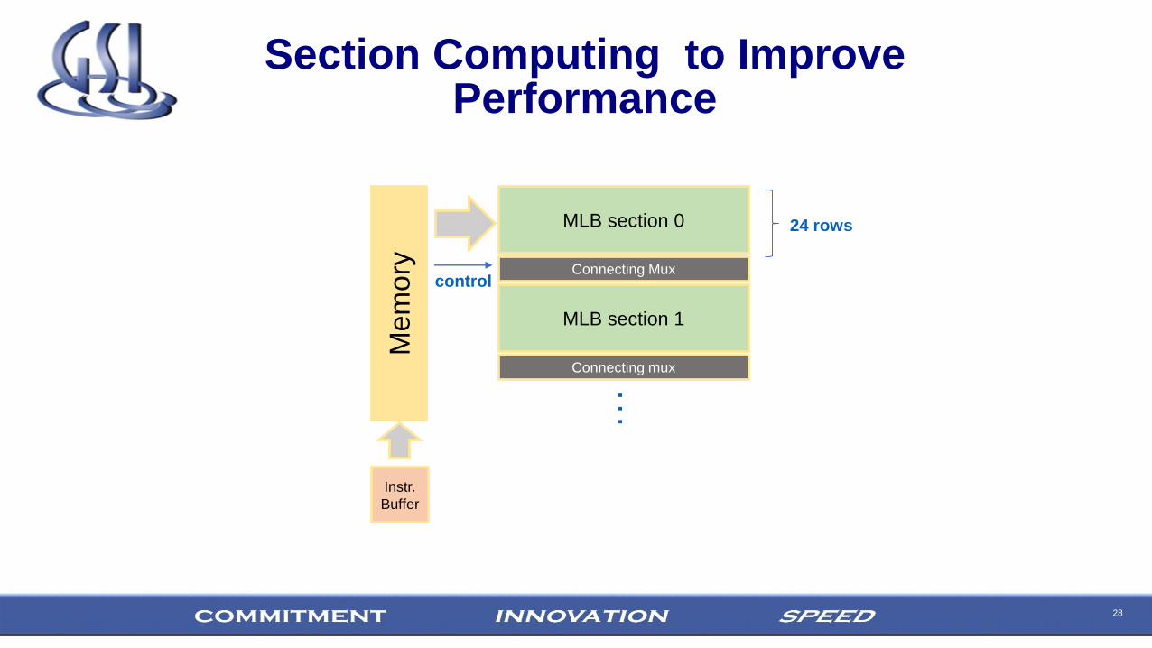
Section Computing to Improve Performance

Mem

ory

MLB section 0

Connecting Mux

. . .

control

Instr.

Buffer

MLB section 1

Connecting mux

24 rows

29

APU Chip Layout

2M bit processors or 128K vector processors runs at 1G Hz

with up to 2 Peta OPS peak performance

30

APU Layout vs GPU Layout

Multi-Functional,

Programmable Blocks

Acceleration of FP

operation Blocks

31

EXAMPLE APPLICATIONS

32

K-Nearest Neighbors (k-NN)

Simple example: N = 36, 3 Groups, 2 dimensions (D = 2 ) for X and Y

K = 4

Group Green selected as the majority

For actual applications: N = Billions, D = Tens, K = Tens of thousands

33

k-NN Use Case in an APU

𝐶𝑝 =𝐷𝑝∙𝑄

𝐷𝑝 𝑄=

σ𝑖=0𝑛 𝐷𝑖

𝑝𝑄𝑖

σ𝑖=0𝑛 𝐷𝑖

𝑝 2σ𝑖=0𝑛 𝑄𝑖

2

Q

4 1 3 2

Majority Calculation

Item features and label

storage

Computing Area

Compute cosine distances

for all N in parallel ( 10s, assuming D=50 features)

K Mins at O(1) complexity ( 3s)

Distribute data – 2 ns (to all)

In-Place ranking

Fe

atu

res o

f item

1

Item 1

Item 2

Item 3

Item N

Fe

atu

res o

f item

2

Fe

atu

res o

f item

N

With the data base in an APU, computation for all N items done in

0.05 ms, independent of K (1000X Improvement over current solutions)

34

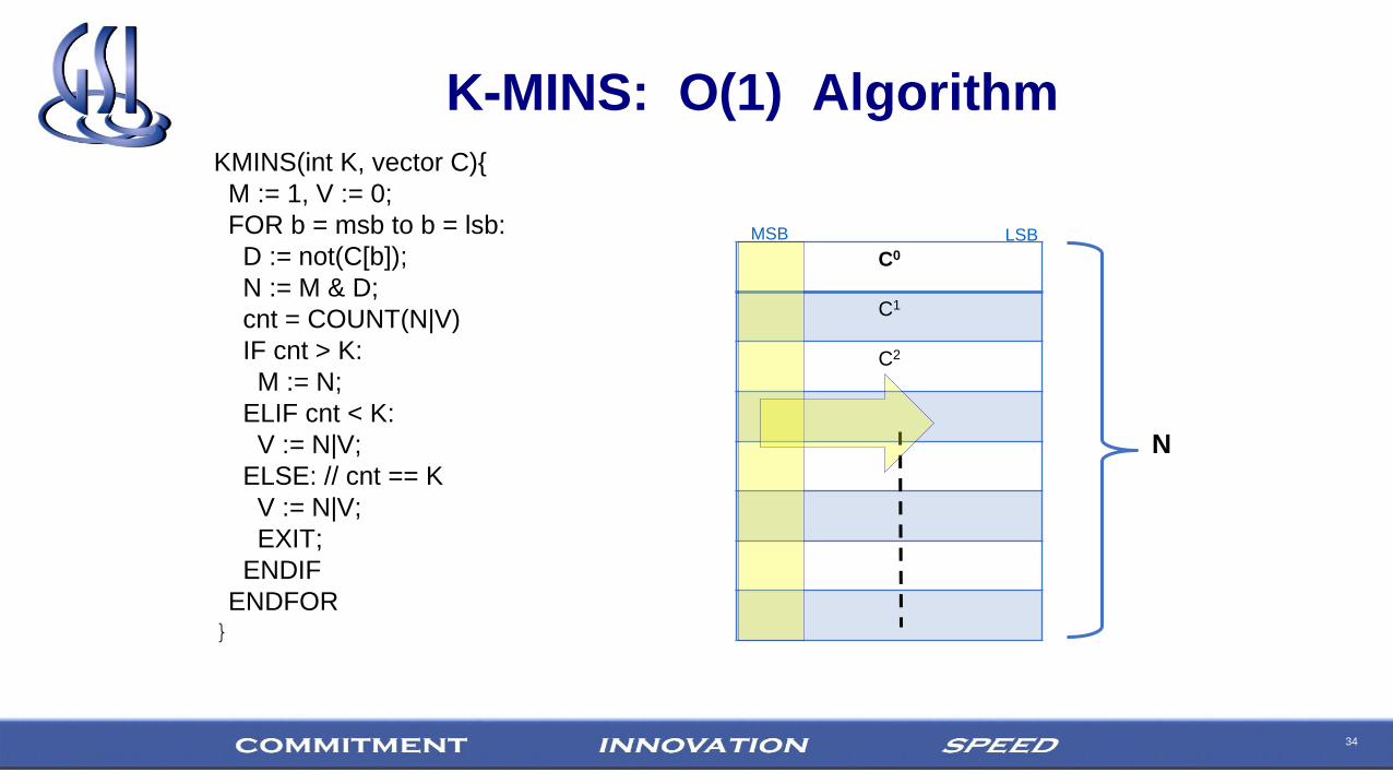
K-MINS: O(1) AlgorithmKMINS(int K, vector C){

M := 1, V := 0;

FOR b = msb to b = lsb:

D := not(C[b]);

N := M & D;

cnt = COUNT(N|V)

IF cnt > K:

M := N;

ELIF cnt < K:

V := N|V;

ELSE: // cnt == K

V := N|V;

EXIT;

ENDIF

ENDFOR}

C0

C1

C2

N

MSB LSB

35

110101

010100

000101

000111

000001

111011

000101

010110

001100

011100

111100

101101

000101

111101

000101

000101

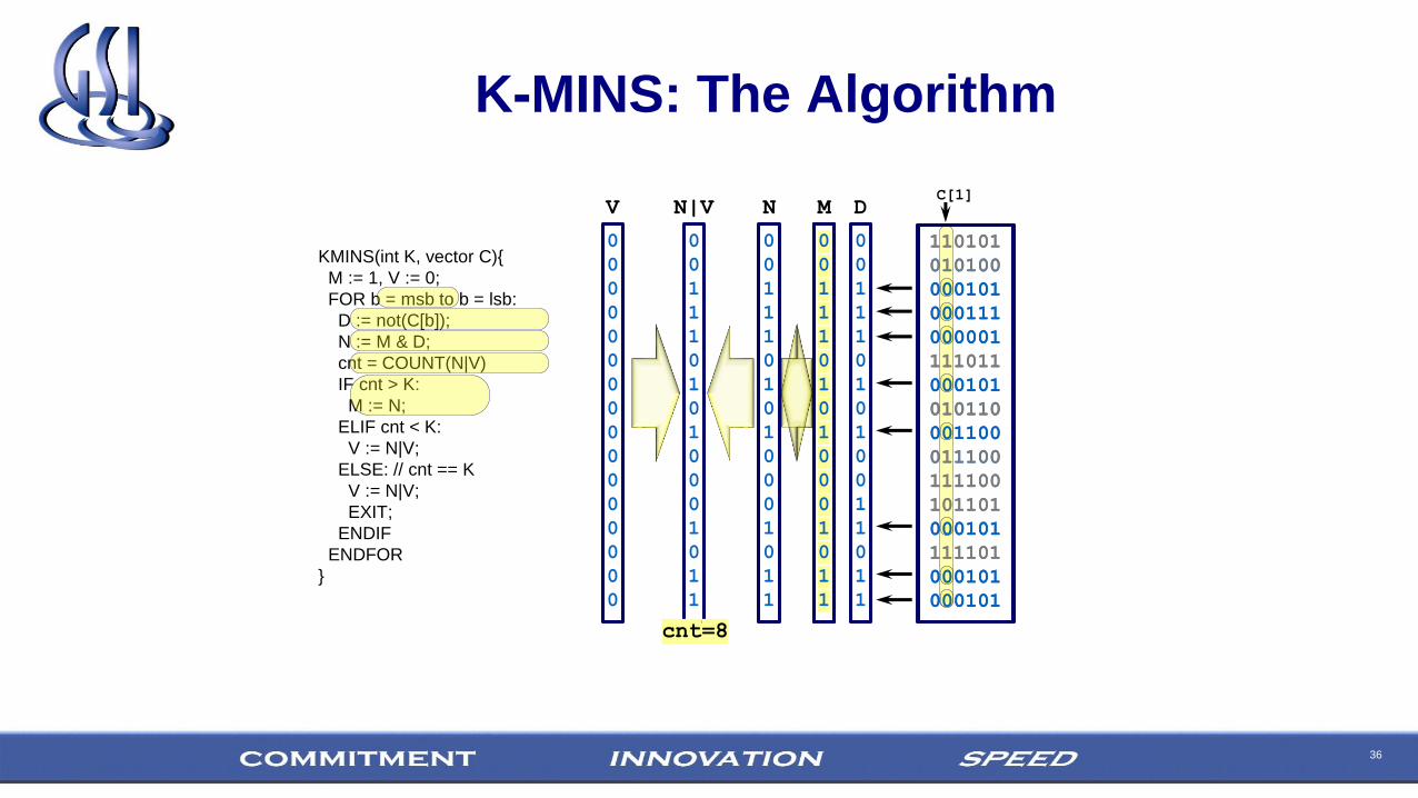
K-MINS: The Algorithm

1

1

1

1

1

1

1

1

1

1

1

1

1

1

1

1

0

0

0

0

0

0

0

0

0

0

0

0

0

0

0

0

V M

KMINS(int K, vector C){

M := 1, V := 0;

FOR b = msb to b = lsb:

D := not(C[b]);

N := M & D;

cnt = COUNT(N|V)

IF cnt > K:

M := N;

ELIF cnt < K:

V := N|V;

ELSE: // cnt == K

V := N|V;

EXIT;

ENDIFENDFOR

}

0

1

1

1

1

0

1

1

1

1

0

0

1

0

1

1

D

0

1

1

1

1

0

1

1

1

1

0

0

1

0

1

1

N

0

1

1

1

1

0

1

1

1

1

0

0

1

0

1

1

N|V

cnt=11

0

1

1

1

1

0

1

1

1

1

0

0

1

0

1

1

110101

010100

000101

000111

000001

111011

000101

010110

001100

011100

111100

101101

000101

111101

000101

000101

C[0]

36

110101

010100

000101

000111

000001

111011

000101

010110

001100

011100

111100

101101

000101

111101

000101

000101

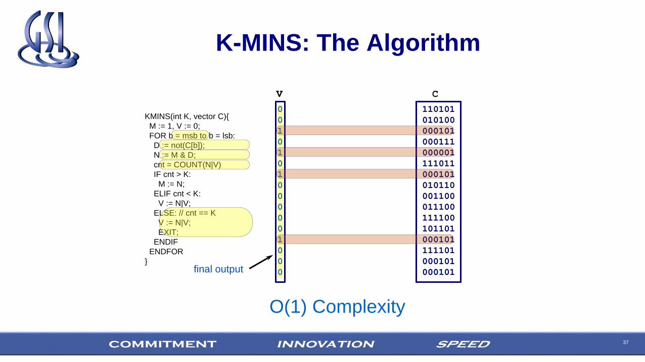
K-MINS: The Algorithm

0

1

1

1

1

0

1

1

1

1

0

0

1

0

1

1

0

0

0

0

0

0

0

0

0

0

0

0

0

0

0

0

V M

KMINS(int K, vector C){

M := 1, V := 0;

FOR b = msb to b = lsb:

D := not(C[b]);

N := M & D;

cnt = COUNT(N|V)

IF cnt > K:

M := N;

ELIF cnt < K:

V := N|V;

ELSE: // cnt == K

V := N|V;

EXIT;

ENDIF

ENDFOR

}

0

0

1

1

1

0

1

0

1

0

0

1

1

0

1

1

D

0

0

1

1

1

0

1

0

1

0

0

0

1

0

1

1

N

0

0

1

1

1

0

1

0

1

0

0

0

1

0

1

1

N|V

cnt=8

0

0

1

1

1

0

1

0

1

0

0

0

1

0

1

1

110101

010100

000101

000111

000001

111011

000101

010110

001100

011100

111100

101101

000101

111101

000101

000101

C[1]

37

110101

010100

000101

000111

000001

111011

000101

010110

001100

011100

111100

101101

000101

111101

000101

000101

K-MINS: The Algorithm

VV

KMINS(int K, vector C){

M := 1, V := 0;

FOR b = msb to b = lsb:

D := not(C[b]);

N := M & D;

cnt = COUNT(N|V)

IF cnt > K:

M := N;

ELIF cnt < K:

V := N|V;

ELSE: // cnt == K

V := N|V;

EXIT;

ENDIF

ENDFOR

}

0

0

1

0

1

0

1

0

0

0

0

0

1

0

0

0

110101

010100

000101

000111

000001

111011

000101

010110

001100

011100

111100

101101

000101

111101

000101

000101

C

final output

O(1) Complexity

38

Similarity Search and Top-K for Recognition

Text

Image

Data BaseEvery image/sentence/doc has a label

Feature Extractor

(Neural network)

Convolution

Layer

Word/Sentence/doc

Embedding

39

Dense (1XN) Vector by Sparse NxM Matrix

4 -2 3 -1

Input Vector

Sparse Matrix

Output Vector

3 5 9 17

1 2 2 4

2 3 4 4

Shift and Add all belonging to same column

0 0 0 0

3 0 0 0

0 5 0 0

0 9 0 17

-6 6 0 -17

Row

Column

-6 15 -9 -17

-6 6 0 -17

Search all columns for row = 2 :Distribute -2 : 2 CySearch all columns for row = 3 :Distribute 3 : 2 Cy Search all columns for row = 4 :Distribute -1 : 2 Cy

Multiply in Parallel : 100 Cy

APU Representations and Computing

-2 3 -1 -1

Complexity including IO : O (N +logβ)

where β is the number of nonzero elements in the sparse matrix

N << M in general for recommender systems

40

Two NxN Sparse Matrix Multiplication

Choose Next free Entry from In-DB1

Read its Row value

Search and Mark Similar Rows

For all Marked Row

Search where Col(In-DB1) = Row(In-DB2)

Broadcast selected value to Output Table bit lines

Multiply in Parallel

Shift and Add all belonging to same Column

Update Out-DB

Go Back to Step 1 if there are more free entries

Exit

Sparse In1 Matrix Sparse Inb-2 Matrix

0 1 0 2 0 0 0 0 3 18 0 34

0 0 0 0 3 0 0 0 0 0 0 0

0 0 6 0 0 5 0 0 0 30 0 0

0 3 0 0 0 9 0 17 9 0 0 0

1 6 3 2 3 5 9 17

2 3 2 4 1 2 2 4

1 3 4 1 2 3 4 4

. . 1 2 2

1

Output Matrix

X =

In-DB1 In-DB2 Out-DB

3 18 34

3 18 34

1 2 4

1 1 1

. 6

30

30

2

3

.9 18 34

3

9

1

4

Complexity Including IO : O(β+logβ) Compared to O(β0.7N1.2 +N2 ) in CPU ( > 1000X Improvement)

COL

ROW

41

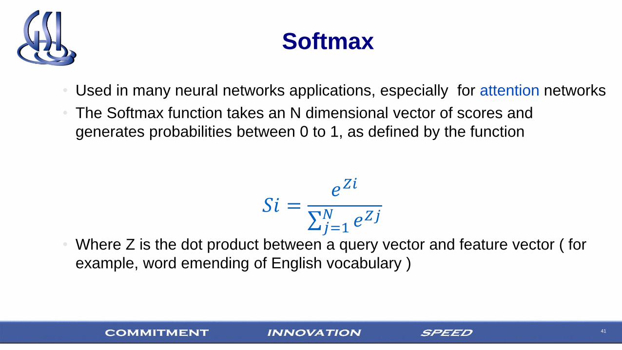
Softmax

• Used in many neural networks applications, especially for attention networks

• The Softmax function takes an N dimensional vector of scores and

generates probabilities between 0 to 1, as defined by the function

• Where Z is the dot product between a query vector and feature vector ( for

example, word emending of English vocabulary )

𝑆𝑖 =𝑒𝑍𝑖

σ𝑗=1𝑁 𝑒𝑍𝑗

42

The Difficulties in Softmax Computing

1. Dot Product for millions vectors

2. Non Linearity function (Exp)

3. Dependency : every score depends on all others in data base

4. Dynamic range: fast overflow, requires high precision calculations

5. Speed and Latency

43

Taylor Series

𝑒𝑥 = 1 + 𝑥 +𝑥2

2+𝑥3

3!+⋯

Very Expensive, Requires more than 20 coefficients and

double precision for good accuracy.

44

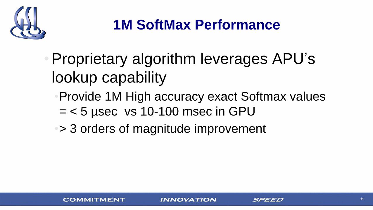
1M SoftMax Performance

• Proprietary algorithm leverages APU’s

lookup capability•Provide 1M High accuracy exact Softmax values

= < 5 µsec vs 10-100 msec in GPU

•> 3 orders of magnitude improvement

45

Associative Memory for Natural Language Processing (NLP)

• Q&A, dialog, language translation, speech recognition etc.

• Requires learning past events

• Needs large array with attention capabilities

46

Examples

• Q&A:

“Dan put the book in his car, ….. Long story

here…. Mike took Dan’s car … Long story here

…. He drove to SF”

• Q : Where is the book now?

• A: Car, SF

• Language Translation:

• “The cow ate the hay because it was delicious”.

• “The cow ate the hay because it was hungry”.

Attention Computing

Source: Łukasz Kaiser

47

Example of Associative Attention Computing

Encoder

(NN)Input Data

(i.e. Sentence in English

for translation or for Q&A)

Fe

atu

re V

ec

tor

Em

be

dd

ing

Sentences Features

Representation (Key)

48

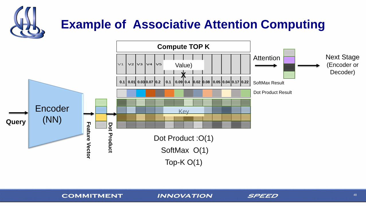
Example of Associative Attention Computing

Encoder

(NN)Query Fe

atu

re V

ec

tor

Do

t Pro

du

ct

Key

Dot Product :O(1)

0.1 0.01 0.03 0.07 0.2 0.1 0.09 0.4 0.02 0.08 0.05 0.04 0.17 0.22

. . .V6V1 V2 V3 V4 V5

X

Attention

Compute TOP K

SoftMax O(1)

Top-K O(1)

Next Stage(Encoder or

Decoder)

Dot Product Result

Value)

SoftMax Result

49

Q&A : End to End Network (Weston)

Source: Weston et

al

50

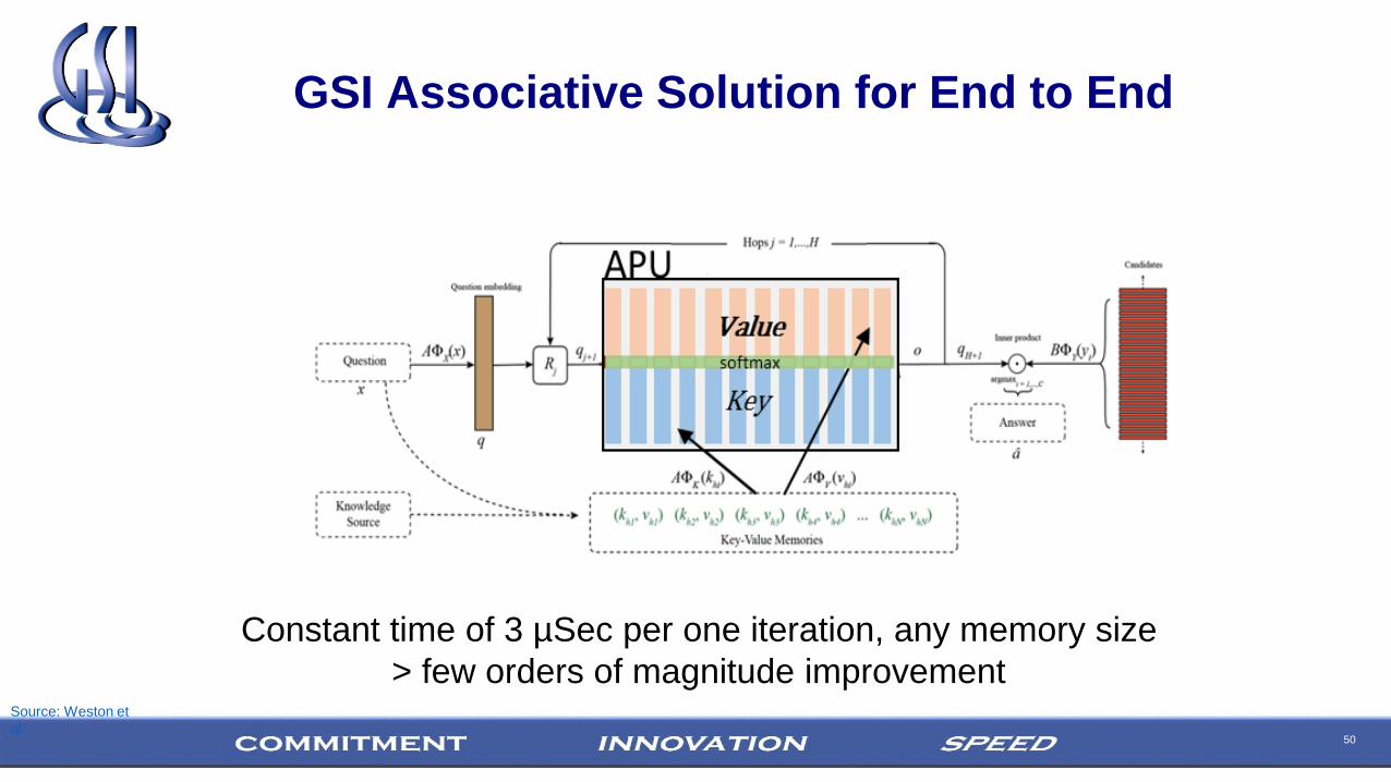
GSI Associative Solution for End to End

Constant time of 3 µSec per one iteration, any memory size

> few orders of magnitude improvementSource: Weston et

al

51

Associative Computing for Low-Shot Learning

• Gradient-Based Optimization has achieved impressive results

on supervised tasks such as image classification

• These models need a lot of data

• People can learn efficiently from few examples

• Associative Computing

• Like people, can measure similarity to features stored in memory

• Can also create a new label for similar features in the future

52

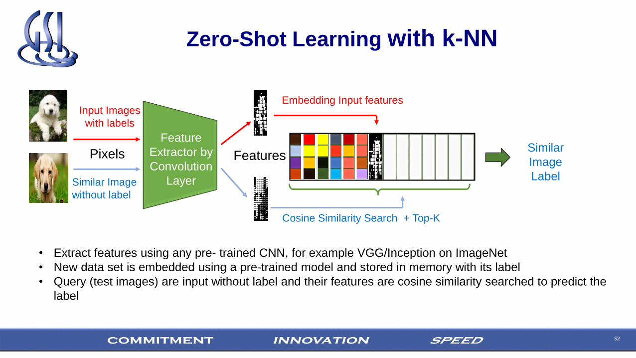
Zero-Shot Learning with k-NN

• Extract features using any pre- trained CNN, for example VGG/Inception on ImageNet

• New data set is embedded using a pre-trained model and stored in memory with its label

• Query (test images) are input without label and their features are cosine similarity searched to predict the

label

Input Images

with labels

Embedding Input features

Pixels Features

Feature

Extractor by

Convolution

Layer

Cosine Similarity Search + Top-K

Similar Image

without label

Similar

Image

Label

53

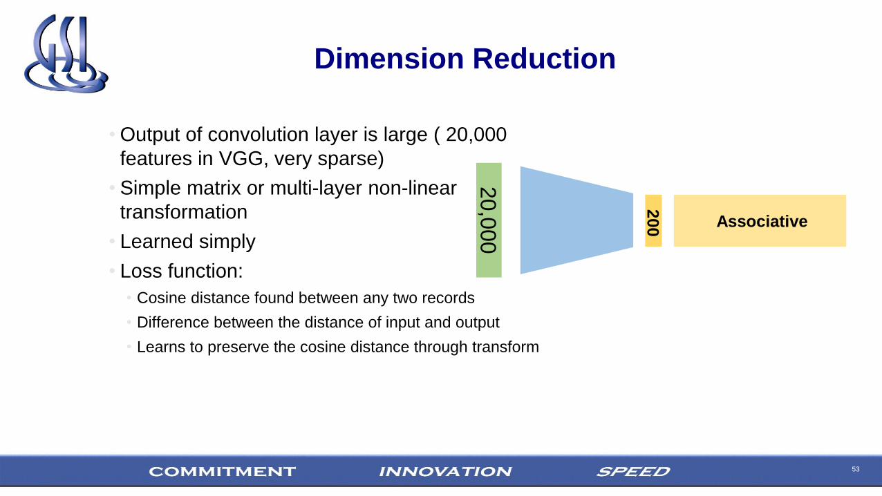
Dimension Reduction

• Output of convolution layer is large ( 20,000

features in VGG, very sparse)

• Simple matrix or multi-layer non-linear

transformation

• Learned simply

• Loss function:

• Cosine distance found between any two records

• Difference between the distance of input and output

• Learns to preserve the cosine distance through transform

20,0

00

200 Associative

54

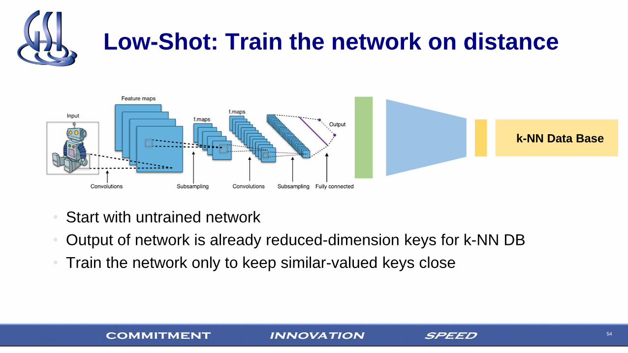
Low-Shot: Train the network on distance

• Start with untrained network

• Output of network is already reduced-dimension keys for k-NN DB

• Train the network only to keep similar-valued keys close

k-NN Data Base

55

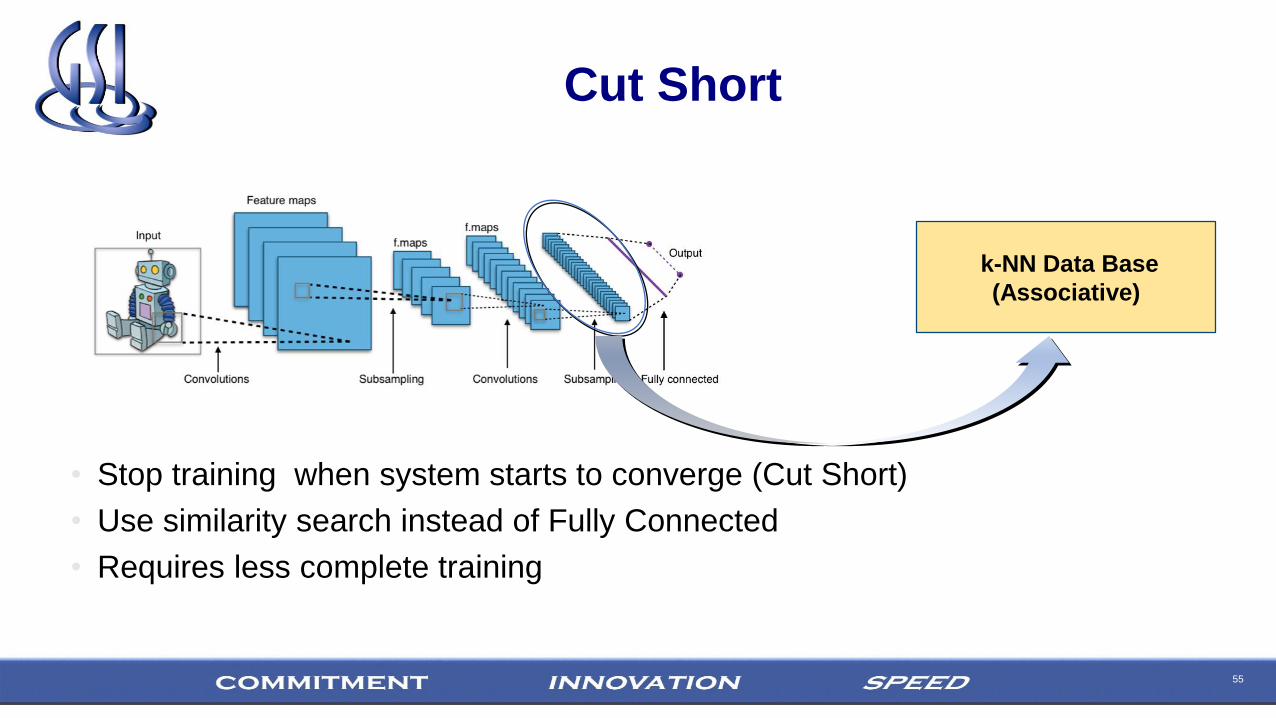
Cut Short

• Stop training when system starts to converge (Cut Short)

• Use similarity search instead of Fully Connected

• Requires less complete training

k-NN Data Base

(Associative)

56

PROGRAMING MODEL

57

Programming Model

Write application In Standard Host Using TensorFlow

/Tesor2Tensor Frame Work

Generates TensorFlow Graph

for Execution in Device

Memory

APU Chip/Card

Execute the

Graph using fused

Capabilities

58

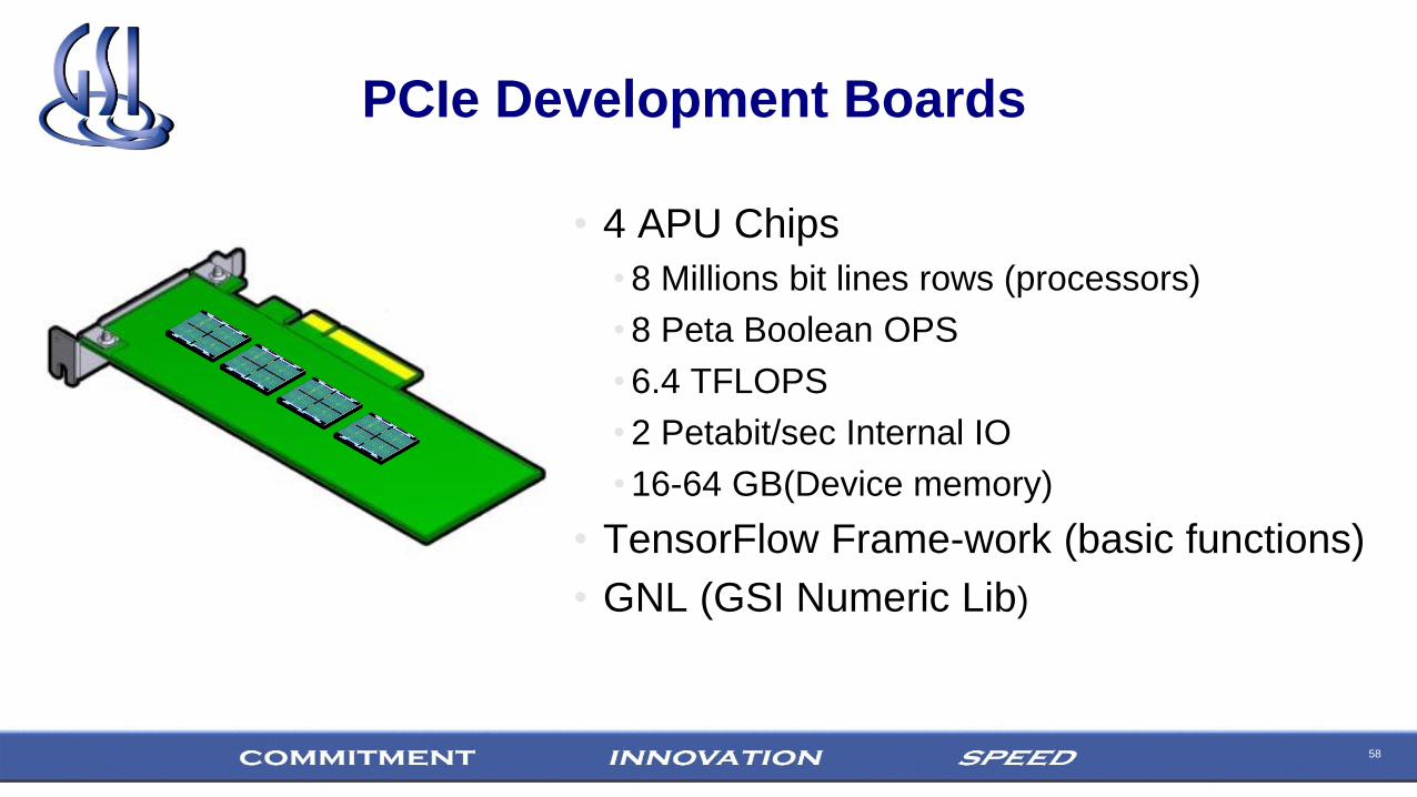
PCIe Development Boards

• 4 APU Chips

• 8 Millions bit lines rows (processors)

• 8 Peta Boolean OPS

• 6.4 TFLOPS

• 2 Petabit/sec Internal IO

• 16-64 GB(Device memory)

• TensorFlow Frame-work (basic functions)

• GNL (GSI Numeric Lib)

59

FUTURE APPROACH – NON VOLATILE CONCEPT

60

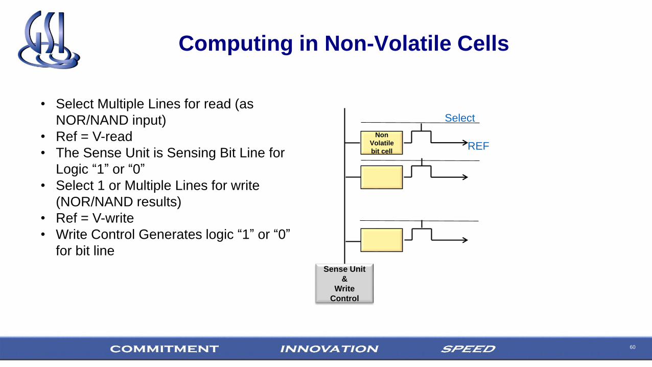
Computing in Non-Volatile Cells

Non

Volatile

bit cell

Sense Unit

&

Write

Control

Select

REF

• Select Multiple Lines for read (as

NOR/NAND input)

• Ref = V-read

• The Sense Unit is Sensing Bit Line for

Logic “1” or “0”

• Select 1 or Multiple Lines for write

(NOR/NAND results)

• Ref = V-write

• Write Control Generates logic “1” or “0”

for bit line

61

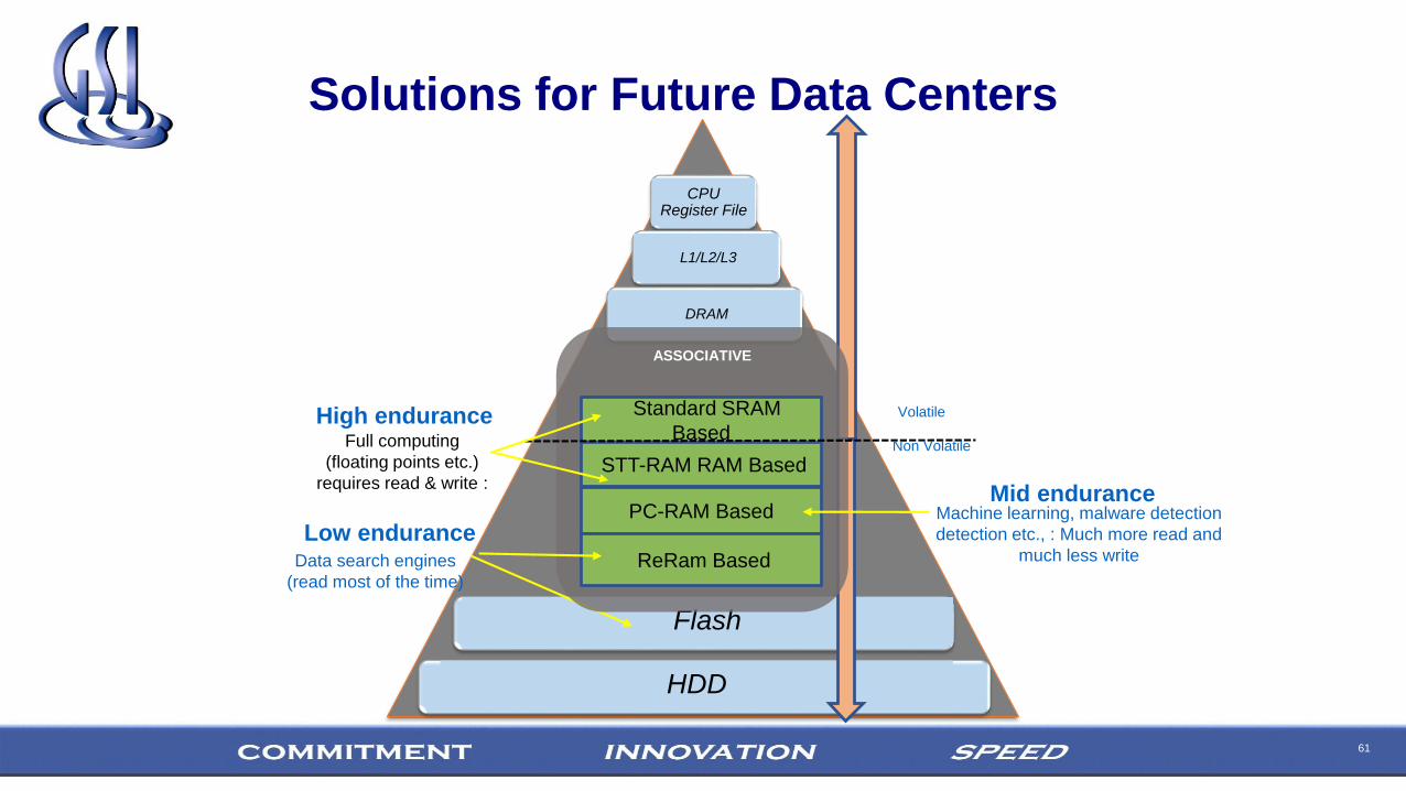
CPU Register File

L1/L2/L3

Flash

HDD

Solutions for Future Data Centers

DRAM

ASSOCIATIVE

STT-RAM RAM Based

PC-RAM Based

ReRam Based

Full computing

(floating points etc.)

requires read & write :

Machine learning, malware detection

detection etc., : Much more read and

much less writeData search engines

(read most of the time)

High endurance

Mid endurance

Low endurance

Standard SRAM

BasedVolatile

Non Volatile

62

Summary

APU enables state of the art, next-generation machine learning :

• In-Place from basic Boolean Algebra to complex algorithms

• O(1) Dot Produces computation

• O(1) Min/Max

• O(1) Top K

• O(1) Softmax

• Ultra high Internal BW – 0.5 Peta bit/sec

• Up to 2 PetaOps of Boolean Algebra in a single chip

• Fully Scalable

• Fully Programmable

• Efficient TensorFlow based capabilities

63

Summary

Extending

Moore’s Law and

Leveraging Advanced Memory Technology Growth

For M.Sc./Ph.D. students that would like to collaborate on

research please contact me:

aakerib@gsitechnology.com

64

Thank You!

Any Questions?

APU Page – http://www.gsitechnology.com/node/123377