Gregory D. Hager Laboratory for Computation, Sensing, and Control Department of Computer Science Johns Hopkins University Perception & Sensing in Robotic Mobility and Manipulation !"#$%&’(#)%" +% ,%-%#)(. The Role of Perception in RMM • Where am I relative to the world? – sensors: vision, stereo, range sensors, acoustics – problems: scene modeling/classification/recognition – integration: localization/mapping algorithms (e.g. SLAM) • What is around me? – sensors: vision, stereo, range sensors, acoustics, sounds, smell – problems: object recognition, structure from x, qualitative modeling – integration: collision avoidance/navigation, learning !"#$%&’(#)%" +% ,%-%#)(. The Role of Perception in RMM • How can I safely interact with environment (including people!)? – sensors: vision, range, haptics (force+tactile) – problems: structure/range estimation, modeling, tracking, materials, size, weight, inference – integration: navigation, manipulation, control, learning • How can I solve “new” problems (generalization)? – sensors: vision, range, haptics, undefined new sensor – problems: categorization by function/shape/context/?? – integrate: inference, navigation, manipulation, control, learning • Obstacle detection, environment interaction •Mapping, registration, localization, recognition • Manipulation Topics Today • Computational Stereo • Feature detection and matching • Motion tracking and visual feedback Techniques Applications in Robotics: !"#$%&’(#)%" +% ,%-%#)(. What is Computational Stereo? Viewing the same physical point from two different viewpoints allows depth from triangulation !"#$%&’(#)%" +% ,%-%#)(. Computational Stereo • Much of geometric vision is based on information from 2 (or more) camera locations – hard to recover 3D information from a single 2D image without extra knowledge – motion and stereo (multiple cameras) are both common in the world • Stereo vision is ubiquitous in nature – (oddly, nearly 10% of people are stereo blind) • Stereo involves the following three problems: 1. calibration 2. matching (correspondence problem) 3. reconstruction (reconstruction problem)
Transcript
Gregory D. Hager
Laboratory for Computation, Sensing, and Control
Department of Computer Science
Johns Hopkins University
Perception & Sensingin Robotic Mobility and Manipulation
!"#$%&'(#)%"*+%*,%-%#)(.
The Role of Perception in RMM
• Where am I relative to the world?– sensors: vision, stereo, range sensors, acoustics
– problems: scene modeling/classification/recognition
• How can I safely interact with environment (includingpeople!)?– sensors: vision, range, haptics (force+tactile)– problems: structure/range estimation, modeling, tracking,
• How can I solve “new” problems (generalization)?– sensors: vision, range, haptics, undefined new sensor– problems: categorization by function/shape/context/??– integrate: inference, navigation, manipulation, control,
learning
• Obstacle detection, environment interaction
•Mapping, registration, localization, recognition
• Manipulation
Topics Today
• Computational Stereo
• Feature detection and matching
• Motion tracking and visual feedback
Techniques
Applications in Robotics:
!"#$%&'(#)%"*+%*,%-%#)(.
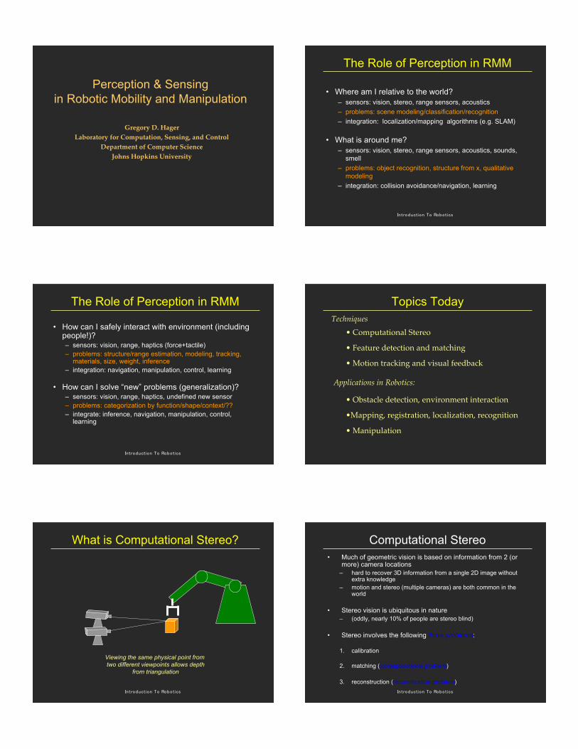
What is Computational Stereo?
Viewing the same physical point from
two different viewpoints allows depth
from triangulation
!"#$%&'(#)%"*+%*,%-%#)(.
Computational Stereo• Much of geometric vision is based on information from 2 (or
more) camera locations– hard to recover 3D information from a single 2D image without
extra knowledge– motion and stereo (multiple cameras) are both common in the
world
• Stereo vision is ubiquitous in nature– (oddly, nearly 10% of people are stereo blind)
• Stereo involves the following three problems:
1. calibration
2. matching (correspondence problem)
3. reconstruction (reconstruction problem)
!"#$%&'(#)%"*+%*,%-%#)(.
Binocular Stereo System: Geometry
• GOAL: Passive 2-camera systemusing triangulation to generate adepth map of a world scene.
• Depth map: z=f(x,y) where x,y arecoordinates one of the imageplanes and z is the height abovethe respective image plane.
– Note that for stereo systems whichdiffer only by an offset in x, the vcoordinates (projection of y) is thesame in both images!
– Note we must convert from image(pixel) coordinates to externalcoordinates -- requires calibration
X
Y
(0,0,f)
4 intrinsic parameters convert
from pixel to metric values
sx sy cx cy!"#$%&'(#)%"*+%*,%-%#)(.
Non-verged Binocular Stereo System
Z
X(0,0) (b,0)
Z=fXL XR
Define Disparity: D = (xL - xR)
Z = b sx
D
Assume: image are scan-line aligned
From perspective projection:xL = sx X/ZxR = sx (X - b)/ZyL = yR = syY/Z
!"#$%&'(#)%"*+%*,%-%#)(.
To increase resolution:• Increase of the baseline
(B) - size of the system
• Increase of the focallength (f) - field of view
• Decrease of the pixel-size(1/sx) - resolution of thecamera
75cm
Stereo-System Accuracy
Z = b sx D
!"#$%&'(#)%"*+%*,%-%#)(.
Two-Camera Geometry
It is not hard to show that when we rotate thecameras inward, corresponding points no longer lie
on a scan line
!"#$%&'(#)%"*+%*,%-%#)(.
How to Change Epipolar Geometry
Image rectification is the computation ofan image as seen by a rotated camera
Original image plane
New image plane
!"#$%&'(#)%"*+%*,%-%#)(.
PlPr
T
Pr = R(Pl – T)
prt E pl = 0
Note that E is invariant to the scale
of the points, therefore we also have
where p denotes the (metric) image
projection of P
Now if K denotes the internal
calibration, converting from metric
to pixel coordinates, we have further
that
rrt K-t
E K-1 rl = rrt F rl = 0
where r denotes the pixel coordinates
of p. F is called the fundamental matrix
Fundamental Matrix Derivation
!"#$%&'(#)%"*+%*,%-%#)(.
Correspondence Problem:
How to find corresponding areas of two cameraimages (points, line segments, curves, regions)
Stereo-Based Reconstruction
!"#$%&'(#)%"*+%*,%-%#)(.
MATCHING AND CORRESPONDENCE
• Two major approaches
– feature-based
– region basedIn feature-based matching, the idea is
to pick a feature type (e.g. edges),define a matching criteria (e.g.
orientation and contrast sign), andthen look for matches within a
disparity range
!"#$%&'(#)%"*+%*,%-%#)(.
Results - Reconstruction
!"#$%&'(#)%"*+%*,%-%#)(.
MATCHING AND CORRESPONDENCE
• Two major approaches
– feature-based
– region based
In region-based matching, theidea is to pick a region in the imageand attempt to find the matchingregion in the second image bymaximizing the some measure: 1. normalized SSD 2. SAD 3. normalized cross-correlation
!"#$%&'(#)%"*+%*,%-%#)(.
Match Metric Summary
I1u,v( ) ! I1( ) " I2 u + d,v( ) ! I2( )
u ,v
#
I1u,v( ) ! I1( )
2
" I2u + d,v( ) ! I2( )
2
u ,v
#u ,v
#
( ) ( )( )! +"vu
vduIvuI
,
2
21,,
( )( )
( )( )
( )( )
( )( )!
!! """"
#
$
%%%%
&
'
(+
(+(
(
(
vu
vuvu
IvduI
IvduI
IvuI
IvuI
,
2
,
2
22
22
,
2
11
11
,
,
,
,
( ) ( )! +"vu
vduIvuI
,
21,,
( ) ( )( )! +"vu
vduIvuI
,
'
2
'
1,,
( ) ( ) ( )! <=nm
kkkvuInmIvuI
,
',,,
( ) ( )( )! +vu
vduIvuIHAMMING
,
'
2
'
1,,,
( ) ( ) ( )( )vuInmIBITSTRINGvuIkknmk,,,
,
'<=
MATCH METRIC DEFINITION
Normalized Cross-Correlation(NCC)
Sum of Squared Differences(SSD)
Normalized SSD
Sum of Absolute Differences(SAD)
Zero Mean SAD
Rank
Census
Remember, these two are actually
the same
( ) ( )! "+""vu
IvduIIvuI
,
_
22
_
11 ),(),(
!"#$%&'(#)%"*+%*,%-%#)(.
Correspondence Search Algorithm
For i = 1:nrows for j=1:ncols
best(i,j) = -1for k = mindisparity:maxdisparity c = ComputeMatchMetric(I1(i,j),I2(i,j+k),winsize) if (c > best(i,j))
best(i,j) = cdisparities(i,j) = k
end end end O(nrows * ncols * disparities * winx * winy)end
I1
I2
u
v
d
I1
I2
u
v
d
!"#$%&'(#)%"*+%*,%-%#)(.
Correspondence Search Algorithm V2
best = -ones(size(im))disp = zeros(size(im))for k = mindisparity:maxdisparity
• Surface structure– lack of texture– repeating texture within horopter bracket
• Geometric ambiguities– as surfaces turn away, difficult to get accurate
reconstruction (affine approximate can help)– at the occluding contour, likelihood of good match
but incorrect reconstruction !"#$%&'(#)%"*+%*,%-%#)(.
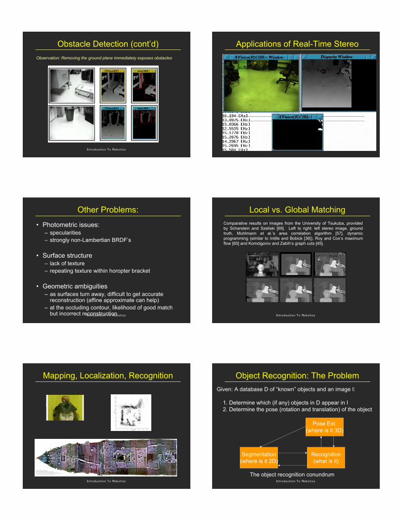
Local vs. Global Matching
Comparative results on images from the University of Tsukuba, providedby Scharstein and Szeliski [69]. Left to right: left stereo image, groundtruth, Muhlmann et al.’s area correlation algorithm [57], dynamicprogramming (similar to Intille and Bobick [36]), Roy and Cox’s maximumflow [65] and Komolgorov and Zabih’s graph cuts [45].
!"#$%&'(#)%"*+%*,%-%#)(.
Mapping, Localization, Recognition
!"#$%&'(#)%"*+%*,%-%#)(.
Object Recognition: The Problem
Given: A database D of “known” objects and an image I:
1. Determine which (if any) objects in D appear in I 2. Determine the pose (rotation and translation) of the object
Segmentation(where is it 2D)
Recognition(what is it)
The object recognition conundrum
Pose Est.(where is it 3D)
!"#$%&'(#)%"*+%*,%-%#)(.
Recognition From Geometry?
Given a database ofobjects and an imagedetermine what, if anyof the objects are present in the image.
!"#$%&'(#)%"*+%*,%-%#)(.
Recognition From Appearance?
• Columbia SLAM system:– can handle databases of 100’s of objects
– single change in point of view
– uniform lighting conditionsCourtesy Shree Nayar, Columbia U.
!"#$%&'(#)%"*+%*,%-%#)(.
Current Best Solution
• Generally view based
• Uses local features and “local” invariance (global istoo weak)
• Uses *lots* of features and some sort of voting
• Also recent attempts to perform “categorical” objectrecognition using similar techniques
• Example: recent papers by Schmid, Lowe, Ponce,Hebert, Perona ...
• Here, we discus SIFT features (Lowe 1999)
!"#$%&'(#)%"*+%*,%-%#)(.
Feature Desiderata
• Features should be distinctive
• Features should be easily detected under changes inpose, lighting, etc.
• There should be many features per object
!"#$%&'(#)%"*+%*,%-%#)(.
Steps in SIFT Feature Selection• Scale-space peak selection
• Keypoint localization– includes rejection due to poor localization– also perform cornerness check using eigenvalues; reject
those with eigenvalue ratio greater than 10
• Orientation Assignment– dominant orientation plus any within 80% of dominant
• Build keypoint descriptor
• Normal images yield approx. 2000 stable features– small objects in cluttered backgrounds require 3-6 features
!"#$%&'(#)%"*+%*,%-%#)(.
Peak Detection
• Find all max and min is LoG images in both space andscale– 8 spatial neighbors; 9 scale neighbors– orientation based on maximum of weighted histogram
!"#$%&'(#)%"*+%*,%-%#)(.
Keypoint Descriptor
!"#$%&'(#)%"*+%*,%-%#)(.
Example
!"#$%&'(#)%"*+%*,%-%#)(.
PDF of Matching
!"#$%&'(#)%"*+%*,%-%#)(.
Feature Matching
• Uses a Hough transform (voting technique)– parameters are position, orientation and scale for
each training view
– features are matched to closest Euclideandistance neighbor in database; each databasefeature indexed to object and view as well aslocation, orientation and scale
– features are linked to adjacent model views; theselinks are also followed and accumulated
– implemented using a hash table
!"#$%&'(#)%"*+%*,%-%#)(.
Results
• Matching requires histogrammingfollowed by alignment
!"#$%&'(#)%"*+%*,%-%#)(.Ponce&Rothganger: 51 test images with 1 to 5