In search of a complex system model : the case of residential mobility Citation for published version (APA): Devisch, O. T. J. (2008). In search of a complex system model : the case of residential mobility Eindhoven: Technische Universiteit Eindhoven DOI: 10.6100/IR632899 DOI: 10.6100/IR632899 Document status and date: Published: 01/01/2008 Document Version: Publisher’s PDF, also known as Version of Record (includes final page, issue and volume numbers) Please check the document version of this publication: • A submitted manuscript is the version of the article upon submission and before peer-review. There can be important differences between the submitted version and the official published version of record. People interested in the research are advised to contact the author for the final version of the publication, or visit the DOI to the publisher's website. • The final author version and the galley proof are versions of the publication after peer review. • The final published version features the final layout of the paper including the volume, issue and page numbers. Link to publication General rights Copyright and moral rights for the publications made accessible in the public portal are retained by the authors and/or other copyright owners and it is a condition of accessing publications that users recognise and abide by the legal requirements associated with these rights. • Users may download and print one copy of any publication from the public portal for the purpose of private study or research. • You may not further distribute the material or use it for any profit-making activity or commercial gain • You may freely distribute the URL identifying the publication in the public portal. If the publication is distributed under the terms of Article 25fa of the Dutch Copyright Act, indicated by the “Taverne” license above, please follow below link for the End User Agreement: www.tue.nl/taverne Take down policy If you believe that this document breaches copyright please contact us at: [email protected]providing details and we will investigate your claim. Download date: 20. May. 2019
Transcript
In search of a complex system model : the case ofresidential mobilityCitation for published version (APA):Devisch, O. T. J. (2008). In search of a complex system model : the case of residential mobility Eindhoven:Technische Universiteit Eindhoven DOI: 10.6100/IR632899
DOI:10.6100/IR632899
Document status and date:Published: 01/01/2008
Document Version:Publisher’s PDF, also known as Version of Record (includes final page, issue and volume numbers)
Please check the document version of this publication:
• A submitted manuscript is the version of the article upon submission and before peer-review. There can beimportant differences between the submitted version and the official published version of record. Peopleinterested in the research are advised to contact the author for the final version of the publication, or visit theDOI to the publisher's website.• The final author version and the galley proof are versions of the publication after peer review.• The final published version features the final layout of the paper including the volume, issue and pagenumbers.Link to publication
General rightsCopyright and moral rights for the publications made accessible in the public portal are retained by the authors and/or other copyright ownersand it is a condition of accessing publications that users recognise and abide by the legal requirements associated with these rights.
• Users may download and print one copy of any publication from the public portal for the purpose of private study or research. • You may not further distribute the material or use it for any profit-making activity or commercial gain • You may freely distribute the URL identifying the publication in the public portal.
If the publication is distributed under the terms of Article 25fa of the Dutch Copyright Act, indicated by the “Taverne” license above, pleasefollow below link for the End User Agreement:
www.tue.nl/taverne
Take down policyIf you believe that this document breaches copyright please contact us at:
Cover design: Ton van Gennip, Tekenstudio Faculteit BouwkundePrinted by the Eindhoven University Press Facilities
CIP-DATA KONINKLIJKE BIBLIOTHEEK, DEN HAAGISBN 90-6814-610-3
i
preface
All started with ‘Swarms and Networks’, an article on the concept of emergence by Kevin Kelly published in 2000 in Oase 53. In this article, Kelly illustrates how the seemingly organized behavior of social animals (such as ant colonies, beehives, bird flocks, sheep herds, etc.) is, contrary to what one would intuitively assume, not necessarily the result of a hierarchical social structure with higher ranks dictating lower ranks, but is, in reality, merely a side-effect of the interaction of a multitude of autonomous individuals, behaving according to self-imposed rules. The point Kelly wants to make in his article is that these interactions can be so synchronous that the group (or colony, hive, flock, herd, or swarm) seems to exhibit own behavior, with features that the constituting group-members do not possess. Kelly gives the example of flocks of birds, turning to avoid predators, where the turning motion travels through the flock as a wave, passing from bird to bird in the space of about one-seventeenth of a second, which is far less than the individual bird’s reaction time. At the moment of reading this article I was doing my architectural internship. Because the concept of emergence did not really help me in drawing technical plans, Kevin Kelly was banned to a place somewhere at the back of my mind. Till I decided to attend a Master of Science in Urban Design at the Bartlett School of Architecture in London. One of the assignments –called Urban Fictions- was to design an Ideal City, a city radically different from our everyday urban spaces, taking on a morphology more akin to that of a forest, a beehive, a space-station, a school of fish, a silicon microchip, a fractal coastline, or a software program. I recalled Kevin Kelly, and never forgot him since. With the help of lecturers like Bill Hillier (Space Syntax) and Michael Batty (Casa), an extensive library, bookshops like Waterstone’s, and the World Wide Web, I made the step from social animals to cities, and started to experiment with computer simulation models such as Boids, Game of Life, Starlogo, Biomorphs, etc. The idea of SwarmCity was born. At the end of my M.Sc. year however, even though I obtained the M.Sc. degree, I could not help but being slightly disappointed: I did discover an extensive and active field of people researching and publishing on the concept of cities as self-organizing systems, but I hardly came across researchers actually implementing this concept in real world settings. To my knowledge, most projects remained theoretical explorations, and those implementations that did exist, were explicitly developed to only illustrate the theoretical concepts, and were, for this reason, deliberately kept abstract. My disappointment made me decide to continue my SwarmCity research, this time not directed at exploring the state of the art, but at actually developing a computer simulation model implementing Kevin Kelly in real world settings. Faith (in the person of Prof. Bruno De Meulder) made me aware that I was not the only one with this ambition, that there even was an open position at the research group of Prof. Harry Timmermans with exactly the same brief. The result is this book: a summary of my four-year journey in the vast world of computer modeling. A journey that would not have been possible without the help of three wise and patient guides,
ii
Prof. Harry Timmermans, Dr. Theo Arentze and Ir. Aloys Borgers, who gave me, a person with no background in modeling, let alone modeling the (location choice) behavior of Dutch people, the opportunity to continue my personal quest. I would especially like to thank Prof. Harry Timmermans, my promoter, for always being there, be it in person or virtually, for giving me endless opportunities, and for letting me spend valuable research-time on tutoring students; Dr. Theo Arentze, my co-promoter, for being a most passionate guide on the subject of behavior-modeling, not only taking time to take me along the conventional paths, but also willing (and even being eager to) leave the beaten track. A guide, who not only showed me where to go, but also learned me how to report –scientifically- on my explorations; Ir. Aloys Borgers, my daily advisor, for introducing me to the peculiarities of the Dutch housing market, and for learning me how to survey and analyze this housing-market. Apart from these three guides, I would like to thank Mandy van de Sande – van Kasteren and Anja van den Elsen – Janssen for their weekly pie-stories and honest concern; and my dear colleagues for their critique and suggestions: a special thank you to Marloes Verhoeven, for her warm hospitality, Sophie Rousseau, for her French energy and cross-cultural friendship, and Michiel Dehaene for being my co-driver and source of inspiration. I would also like to thank my eternal guide and mentor, Prof. Bruno De Meulder, whose mission it seems to be always reside ‘off the map’, a mission, onto which I am proud to be -now and then- invited. I am very grateful to my parents, thanks to whom this journey started in the first place. They not only supported my year in London, but also convinced me to actually apply for the PhD position. And then there is Karin, my loved one, with whom I will get married as this book is being published. I thank her for making me feel proud of my research, but most of all for making me realize that there is a world beyond my computer.
iii
cOntents
Preface
List of Figures
List of Tables
§ 1 Introduction
About planners and models 1
swarm + city 2
Complex system models 3
Context: MASQUE 4
Research-scope 5
Outline of the thesis 6
part I: cOLLectInG cOncepts & cHaLLenGes
§ 2 About household location-choice behavior
Introduction 8
Review of empirical findings 9
Review of operational models 17
Conclusions and discussion 26
part II: fraMeWOrK anD IMpLeMentatIOn
§ 3 Conceptual framework – towards more complexity
Unboundedly rational students / stationary housing-market 90
Unboundedly rational students / non-stationary housing-market 112
Boundedly rational students / non-stationary housing-market 127
Pro-active boundedly rational students / non-stationary housing-market 160
Pro-active boundedly rational students / non-stationary interactive 173 housing-market
Summary 192
v
§ 7 Conclusions and discussion
Introduction 194
Summary of the swarmCity model 195
Discussion: validation 196
Possible directions of future research 200
Bibliography
Appendix
Author index
Subject index
Samenvatting (Dutch summary)
Curriculum vitae
vi
LIst Of fIGUres
Figure 3.1: The different swarmCity agents that take part in the model: an individual (i.e. a household-member), a household and a real-estate firm
Figure 3.2: Composition of the housing-market: the housing-market as a whole, a neighborhood, a parcel and a house
Figure 3.3: Actions a household can undertake: (a) moving, (b) renovating, (c) renting out rooms, (d) investing and (e) doing nothing
Figure 3.4: Basic decision process
Figure 3.5: Graph illustrating the occurrence of a sudden event (the dashed line) and a continuous process (the full line)
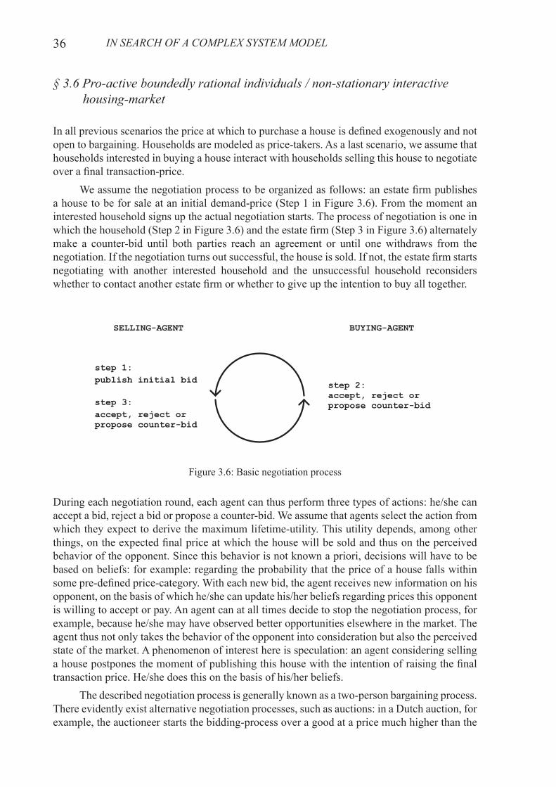
Figure 3.6: Basic negotiation process
Figure 4.1: General structure of a Decision Table (figure from Verhelst, 1980)
Figure 4.2: Example of an Activity Diagram (figure from Gooch, 2000)
Figure 4.3: General structure of a Decision Tree; left with a decision node (represented as a square), right as a nature node (represented as a circle)
Figure 4.4: Example of a Decision Tree with two levels
Figure 4.5: Mental representation of the housing-market by an unboundedly rational individual
Figure 4.6: Activity Diagram of an unboundedly rational individual in a stationary housing-market
Figure 4.7: Decision Tree illustrating the decision of an unboundedly rational individual
Figure 4.8: Activity Diagram of an unboundedly rational individual in a non-stationary housing-market
Figure 4.9: Mental representation of the housing-market by a boundedly rational individual
Figure 4.10: Activity Diagram of a boundedly rational individual in a non-stationary housing-market
Figure 4.11: Decision Tree illustrating the decision of a boundedly rational individual to search, visit, or stay
Figure 4.12: First node in the search-branch of the Decision Tree
Figure 4.13: First and second node in the search-branch of the Decision Tree
Figure 4.14: First, second and third node in the search-branch of the Decision Tree
Figure 4.15: Mental representation of the housing-market by a pro-active boundedly rational individual
Figure 4.16: Decision Tree illustrating the decision of a pro-active boundedly rational individual to search, visit, move or stay
vii
Figure 4.17: Activity Diagram of a pro-active boundedly rational individual in an interactive non-stationary housing-market
Figure 4.18: Mental representation of the housing-market and fellow agents by a pro-active boundedly rational individual
Figure 4.19: Decision Tree illustrating the decision of a pro-active boundedly rational individual to search, visit, negotiate or stay
Figure 4.20: Decision Tree of a real-estate firm
Figure 4.21: Interaction-Sequence-Diagram illustrating the negotiation process
Figure 4.24: Example of a Conditional Probability Table, expressing the beliefs of a buying-agent regarding the probability that a selling-agent would make a bid, conditional on his rejection-price
Figure 4.25: Selling-agent defining a bid in the case where an agent can only accept or reject this bid (figure based on Tryfos, 1981)
Figure 4.26: Selling-agent defining a bid in the case where an agent can accept, reject, and propose a counter-bid
Figure 5.1: UML class-diagram visualizing the relation among all swarmCity objects
Figure 5.2: Eindhoven consists of 106 neighborhoods
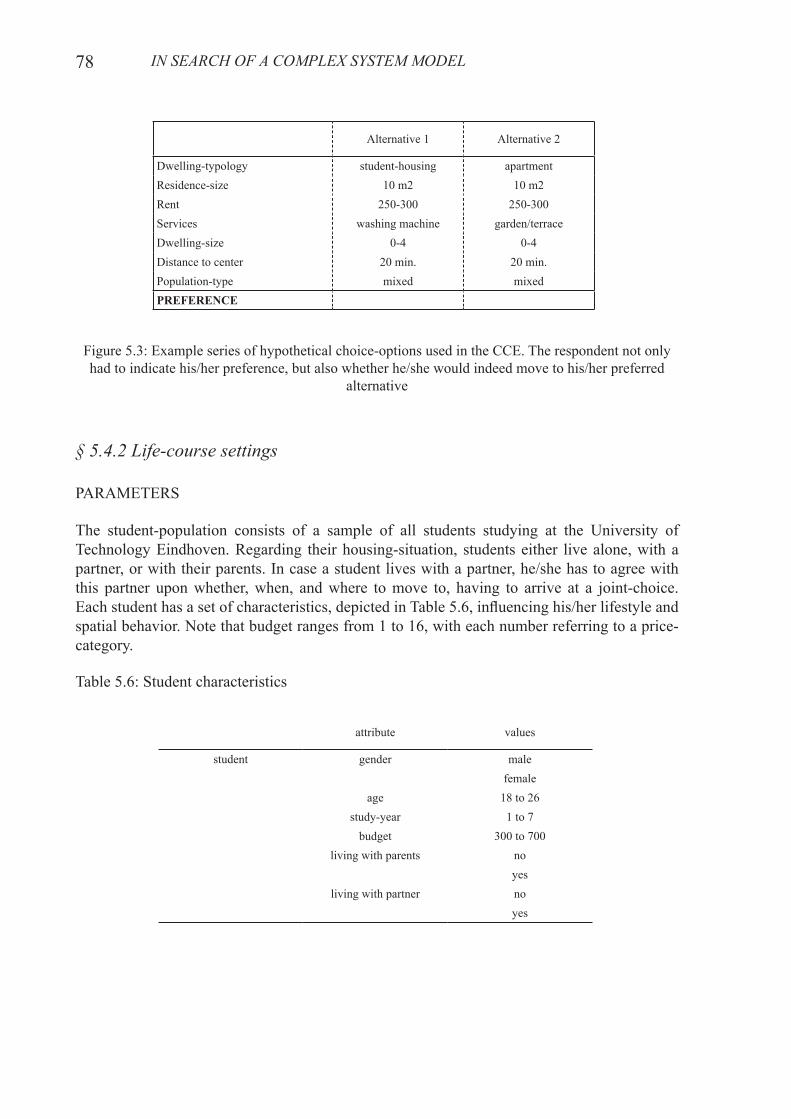
Figure 5.3: Example series of hypothetical choice-options used in the CCE. The respondent not only had to indicate his/her preference, but also whether he/she would indeed move to his/her preferred alternative
Figure 6.1: Decision Table of a student with preference-profile 2
Figure 6.2: Decision Tree, with resistance to change set to zero; o0 represents the parental home
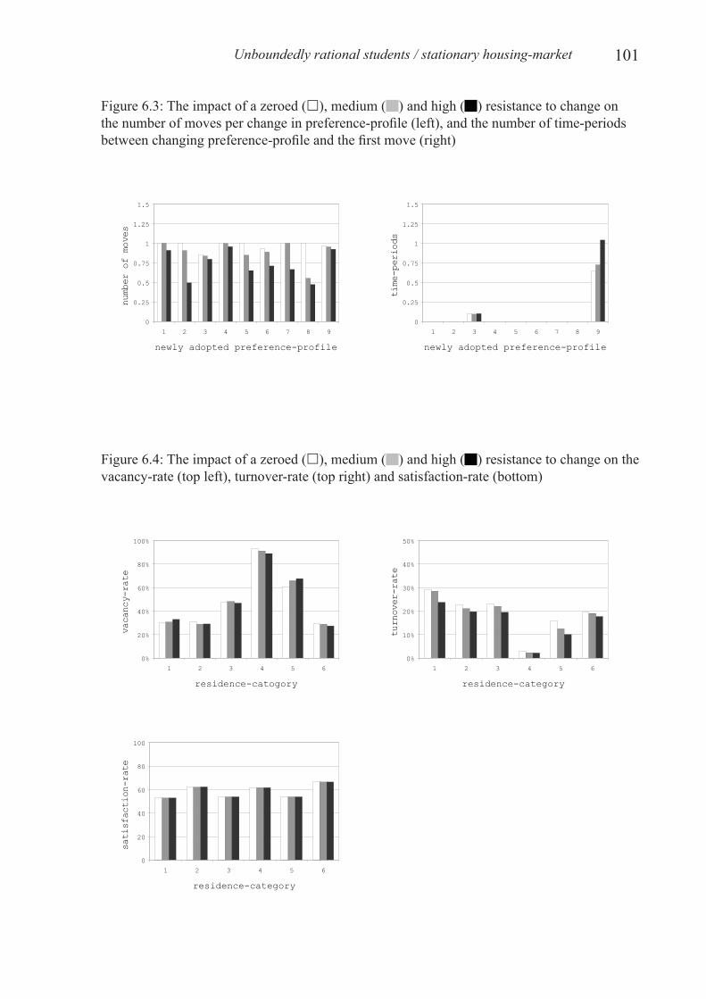
Figure 6.3: The impact of a zeroed, medium and high resistance to change on the number of moves per change in preference-profile (left), and the number of time-periods between changing preference-profile and the first move (right)
Figure 6.4: The impact of a zeroed, medium and high resistance to change on the vacancy-rate (top left), turnover-rate (top right) and satisfaction-rate (bottom)
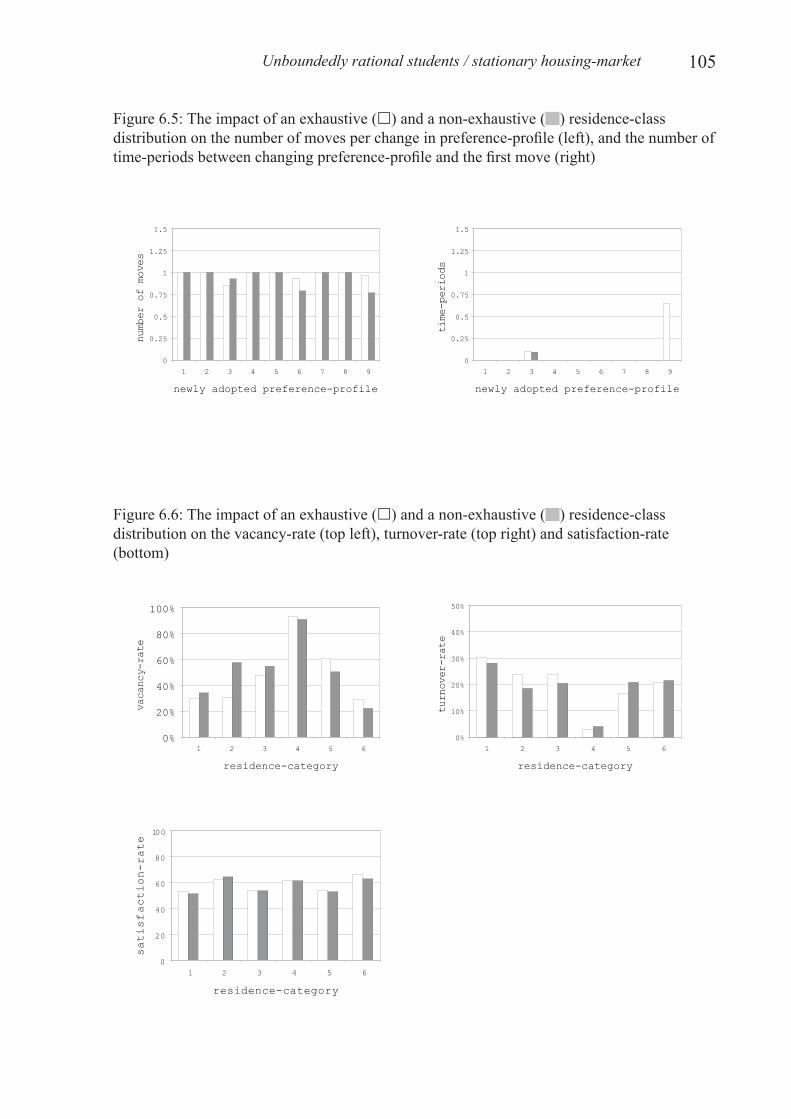
Figure 6.5: The impact of an exhaustive and a non-exhaustive residence-class distribution on the number of moves per change in preference-profile (left), and the number of time-periods between changing preference-profile and the first move (right)
Figure 6.6: The impact of an exhaustive and a non-exhaustive residence-class distribution on the vacancy-rate (top left), turnover-rate (top right) and satisfaction-rate (bottom)
viii
Figure 6.7: The impact of a low and high supply on the number of moves per change in preference-profile (left), and the number of time-periods between changing preference-profile and the first move (right)
Figure 6.8: The impact of a low and high supply on the vacancy-rate (top left), turnover-rate (top right) and satisfaction-rate (bottom)
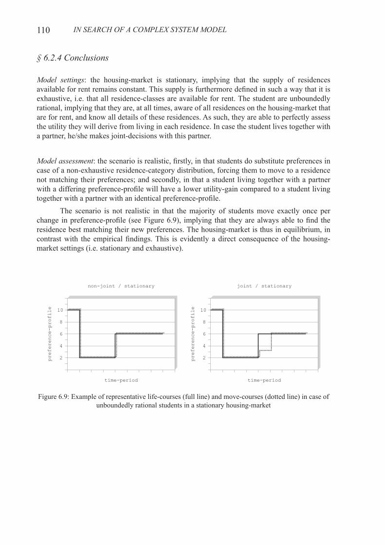
Figure 6.9: Example of representative life-courses (full line) and move-courses (dotted line) in case of unboundedly rational students in a stationary housing-market
Figure 6.10: The impact of a zeroed, medium and high resistance to change on the number of moves per change in preference-profile (left), and the number of time-periods between changing preference-profile and the first move (right)
Figure 6.11: The impact of a zeroed, medium and high resistance to change on the vacancy-rate (top left), turnover-rate (top right) and satisfaction-rate (bottom)
Figure 6.12: The impact of an exhaustive and a non-exhaustive residence-class distribution on the number of moves per change in preference-profile (left), and the number of time-periods between changing preference-profile and the first move (right)
Figure 6.13: The impact of an exhaustive and a non-exhaustive residence-class distribution on the vacancy-rate (top left), turnover-rate (top right) and satisfaction-rate (bottom)
Figure 6.14: The impact of a low and high supply on the number of moves per change in preference-profile (left), and the number of time-periods between changing preference-profile and the first move (right)
Figure 6.15: The impact of a low and high supply on the vacancy-rate (top left), turnover-rate (top right) and satisfaction-rate (bottom)
Figure 6.16: Example of a representative life-course (full line) and move-course (dotted line) in case of unboundedly rational students in a non-stationary housing-market
Figure 6.17: Activity Diagram of the student-case, in case of boundedly rational students
Figure 6.18: Decision Table of a student with preference-profile 2
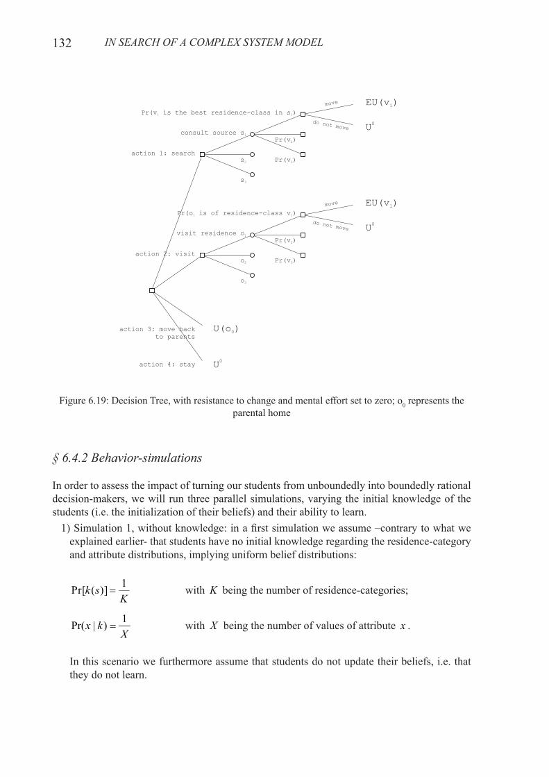
Figure 6.19: Decision Tree, with resistance to change and mental effort set to zero; o0 represents the parental home
Figure 6.20: The impact of a zeroed, z∆ , a b∆ , and an overall resistance to change on the number of moves per change in preference-profile (left), and the number of time-periods between changing preference-profile and the first move (right)
Figure 6.21: The impact of a zeroed, a z∆ , a b∆ , and an overall resistance to change on the vacancy-rate (top left), turnover-rate (top right), satisfaction-rate (bottom left) and advertisement-period (bottom right)
Figure 6.22: The impact of an exhaustive and a non-exhaustive residence-class distribution on the number of moves per change in preference-profile (left), and the number of time-periods between changing preference-profile and the first move (right)
ix
Figure 6.23: The impact of an exhaustive and a non-exhaustive residence-class distribution on the vacancy-rate (top left), turnover-rate (top right), satisfaction-rate (bottom left) and advertisement-period (bottom right)
Figure 6.24: The impact of a low and high supply on the number of moves per change in preference-profile (left), and the number of time-periods between changing preference-profile and the first move (right)
Figure 6.25: The impact of a low and high supply on the vacancy-rate (top left), turnover-rate (top right), satisfaction-rate (bottom left) and advertisement-period (bottom right)
Figure 6.26: Example of a representative life-course (full line) and move-course (dotted line) in case of boundedly rational students in a non-stationary housing-market
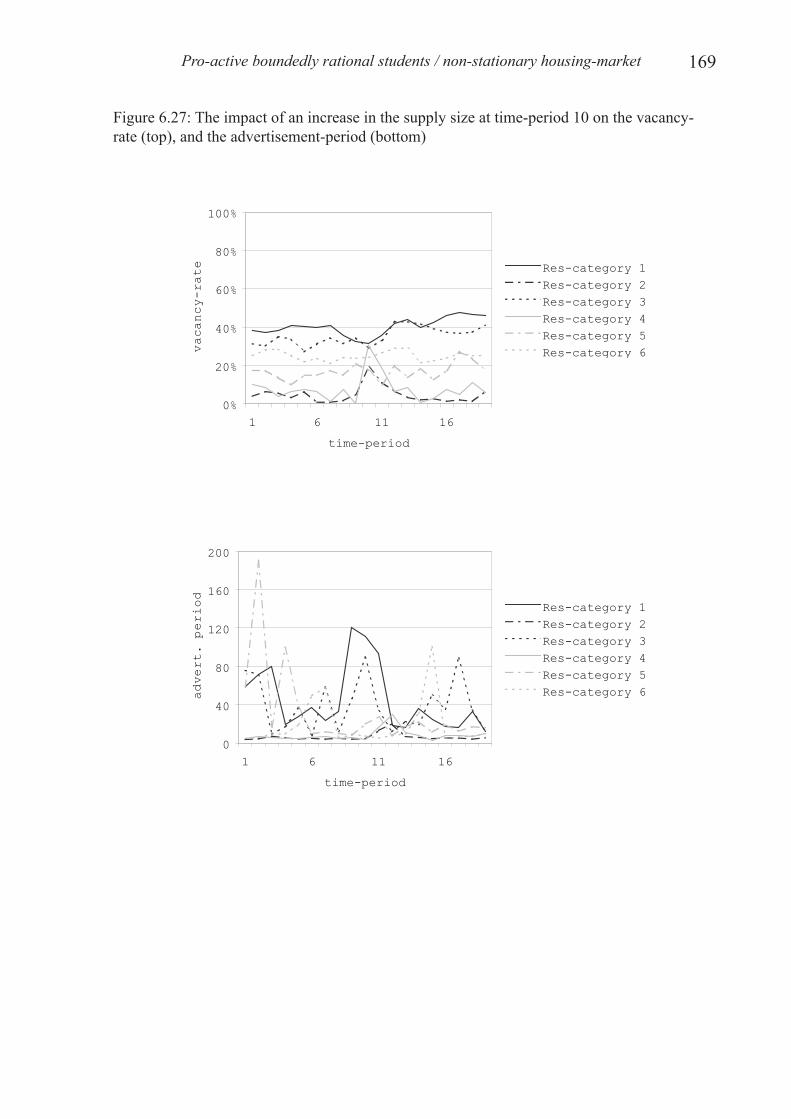
Figure 6.27: The impact of an increase in the supply size at time-period 10 on the vacancy-rate (top), and the advertisement-period (bottom)
Figure 6.28: The impact of an increase in resistance to move at time-period 13 on the vacancy-rate (top), and the advertisement-period (bottom)
Figure 6.29: Example of a representative life-course (full line) and move-course (dotted line) in case of pro-active boundedly rational students in a non-stationary housing-market
Figure 6.30: Activity Diagram of the student-case, in case of an interactive housing-market
Figure 6.31: Acceptance-belief distribution and expected rent )(" kc of a student for a given residence-category k
Figure 6.32: Decision Table of a student with preference-profile 2
Figure 6.33: Decision Tree, with resistance to change and mental effort set to zero; 0o represents the parental home
Figure 6.34: The impact of a low and a high supply on the rent-evolution. Results are grouped according to residence-category
Figure 6.35: The impact of the initial belief-distribution on the evolution of the initial demand-price of both the landlords and the students, and on the final transaction rent
Figure 6.36: The impact of the delay-costs on the evolution of the initial demand-price of both the landlords and the students, and on the final transaction rent
Figure 6.37: Life- (full line) and move-courses (dotted line) of students under different scenarios
x
LIst Of tabLes
Table 5.1: Housing-market characteristics
Table 5.2: Residence-categories
Table 5.3: University statistics regarding gender, marital status and housing-situation
Table 5.4: University statistics regarding the number of years it takes students, on average, to finish their student career
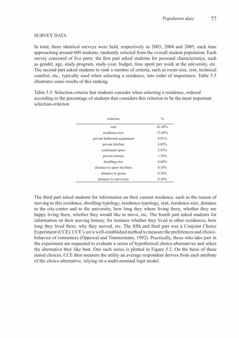
Table 5.5: Selection-criteria that students consider when selecting a residence, ordered according to the percentage of students that considers this criterion to be the most important selection-criterion
Table 5.6: Student characteristics
Table 5.7: Student-profiles
Table 5.8: Example of a transition matrix, specifying the probability that a student who has been living with a partner for the last two years, will or will not keep on living with a partner over the next three years
Table 5.9: Transition matrix summarizing all possible student-profile transitions
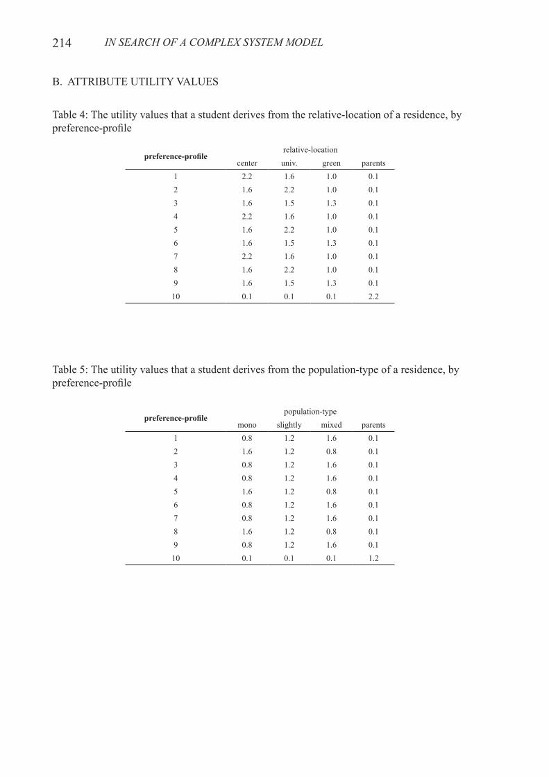
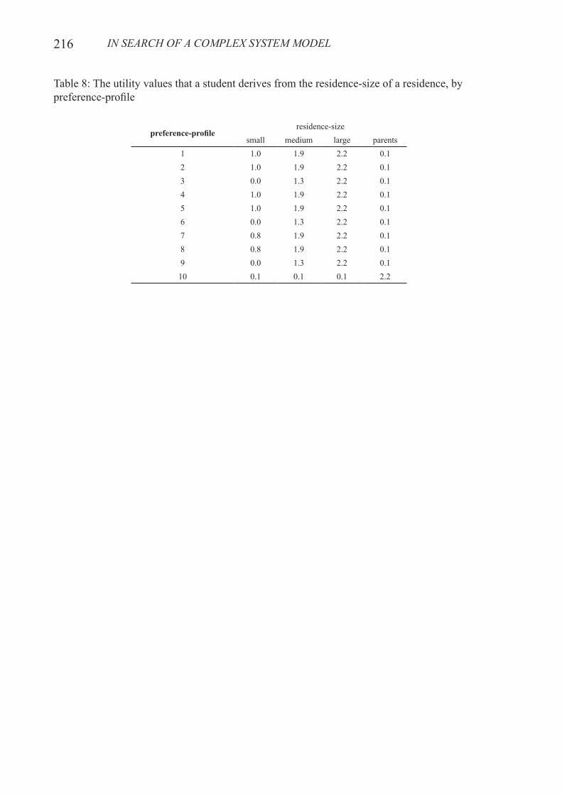
Table 5.10: The 10 preference-profiles and their preferred housing-market characteristics
Table 5.11: Distribution of the preference-profiles over the different student-profiles, and this for a male student
Table 5.12: Example of utility values, specifying the utility that a student derives from the relative location of a residence, by preference-profile. The column ‘parents’ is added to let students evaluate the utility of moving back to the parental home
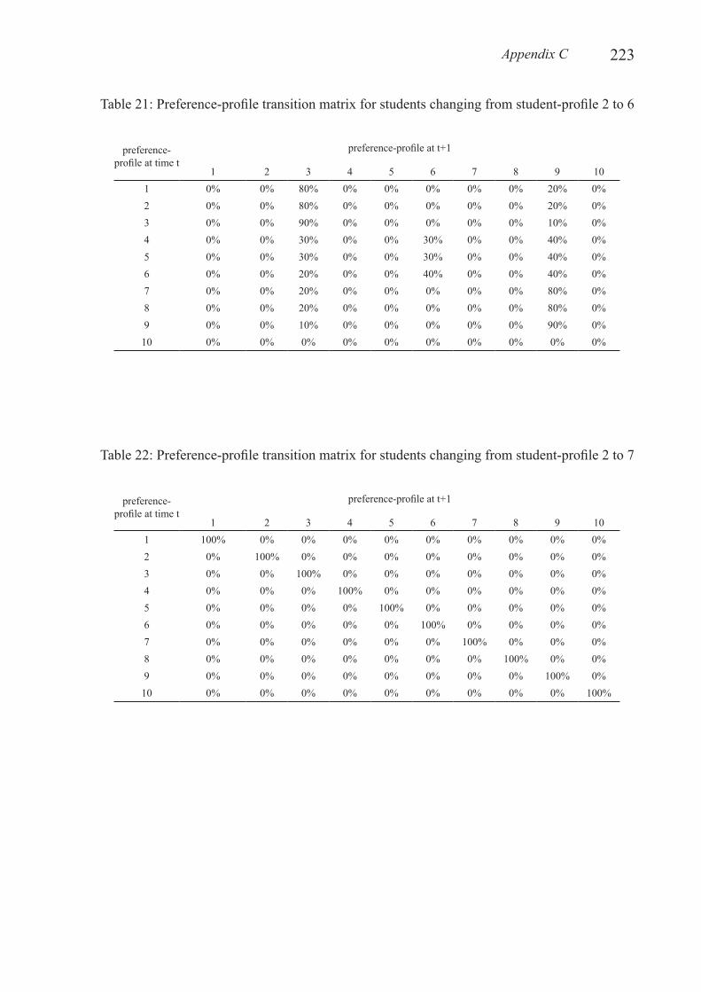
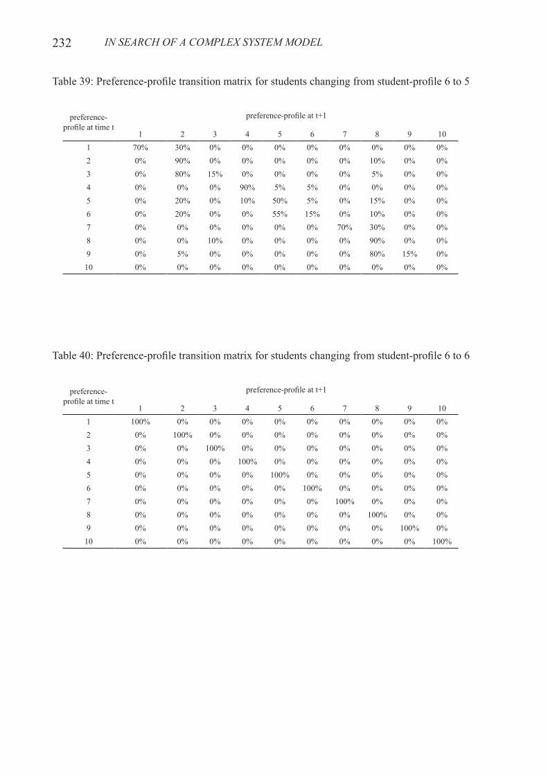
Table 5.13: Example of a preference-profile transition matrix, i.e. for students changing from student-profile 1 to 2
Table 5.14: Preference-profile distribution of those residences the student population lives in at the beginning of the simulation. The extra supply of new residences available for rent is not included
Table 5.15: Probability that any student undergoes a particular life-course change
Table 5.16: Probability that any student changes to a particular preference-profile
Table 6.1: Average results on the level of the whole population. In the scenario without joint decision-making, only the moving behavior of the male students is recorded
Table 6.2: Number of moves per change in preference-profile
Table 6.3: Average increase in utility related to the first move after changing preference-profile
Table 6.4: The distribution of preference-profiles matching the final residence the students moved to, without joint decision-making (above the line) and with joint decision-making (below the line)
xi
Table 6.5: Number of time-periods between changing preference-profile and the first move
Table 6.6: The life- and move-course of student 3459, without joint decision-making (above the line) and with joint decision-making (below the line)
Table 6.7: The life- and move-course of student 4312
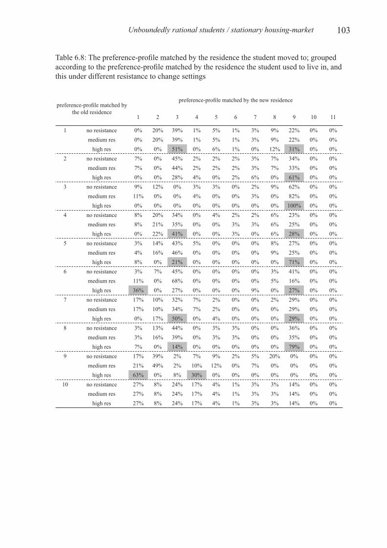
Table 6.8: The preference-profile matched by the residence the student moved to; grouped according to the preference-profile matched by the residence the student used to live in, and this under different resistance to change settings
Table 6.9: Preference-profile distribution in case of an exhaustive and a non-exhaustive distribution, over the whole housing-market
Table 6.10: The distribution of preference-profiles matching the final residence the students moved to, in case of a non-exhaustive distribution
Table 6.11: The life- and move-course of student 3872; in case of a non-exhaustive distribution
Table 6.12: The life- and move-course of student 3515; in case of a low and high supply
Table 6.13: The distribution of preference-profiles matching the final residence the students moved to, in case of a low supply
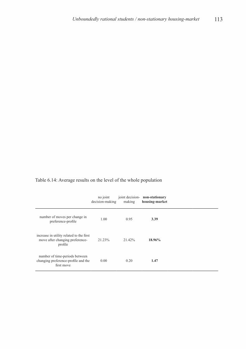
Table 6.14: Average results on the level of the whole population
Table 6.15: Average competition on the housing-market, per preference-profile
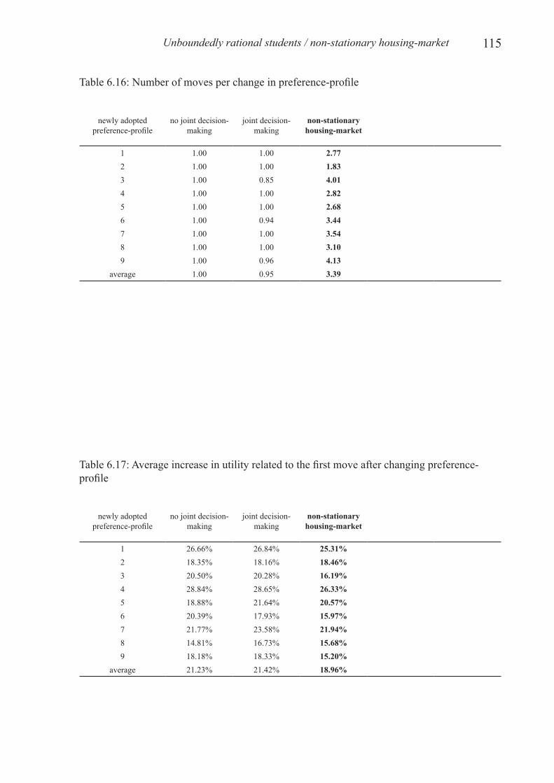
Table 6.16: Number of moves per change in preference-profile
Table 6.17: Average increase in utility related to the first move after changing preference-profile
Table 6.18: The distribution of the preference-profiles matching the final residence the students moved to
Table 6.19: Number of time-periods between changing preference-profile and the first move
Table 6.20: The life- and move-course of student 3734
Table 6.21: The life- and move-course of student 3501
Table 6.22: Initial residence-category distribution for each information-source and for the housing-market as a whole
Table 6.23: Initial attribute-beliefs on the overall housing-market, irrespective of residence-category
Table 6.24: Average results on the level of the whole population
Table 6.25: Number of moves per change in preference-profile
xii
Table 6.26: Average increase in utility related to the first move after changing preference-profile
Table 6.27: The distribution of preference-profiles matching the final residence the students moved to
Table 6.28: Number of time-periods between changing preference-profile and the first move
Table 6.29: Number of visits between changing preference-profile and the first move
Table 6.30: The complete life- and move-course of student 3428
Table 6.31: A fragment of the life- and move-course of student 3427
Table 6.32: The first part of the life- and move-course of student 3526
Table 6.33: The last part of the life- and move-course of student 3503
Table 6.34: Initial residence-category distribution for each information-source and for the housing-market as a whole, in case of regular sources
Table 6.35: Number of moves per change in preference-profile, in case of regular sources
Table 6.36: Average increase in utility related to the first move after changing preference-profile, in case of regular sources
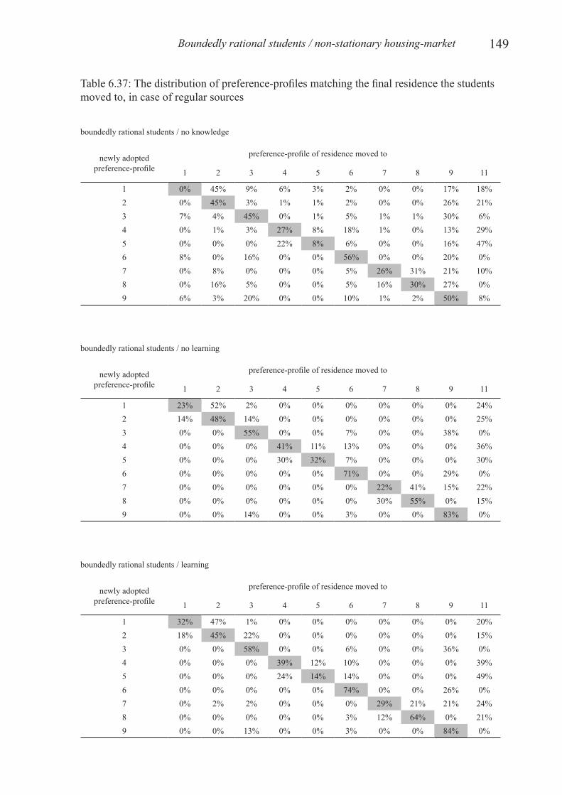
Table 6.37: The distribution of preference-profiles matching the final residence the students moved to, in case of regular sources
Table 6.38: Number of time-periods between changing preference-profile and the first move, in case of regular sources
Table 6.39: Number of visits between changing preference-profile and the first move, in case of regular sources
Table 6.40: The complete life- and move-course of student 3922
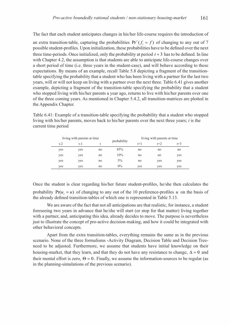
Table 6.41: Example of a transition-table specifying the probability that a student who stopped living with his/her parents, moves back to his/her parents over the next three years; t is the current time period.
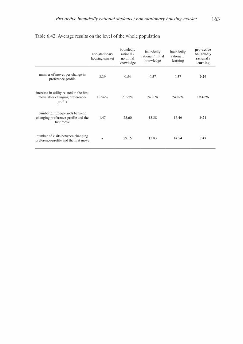
Table 6.42: Average results on the level of the whole population
Table 6.43: A fragment of the life- and move-course of student 3835
Table 6.44: A fragment of the life- and move-course of student 3887
Table 6.45: A fragment of the life- and move-course of student 3894
Table 6.46: A fragment of the life- and move-course of student 3840
Table 6.47: A fragment of the life- and move-course of student 3920
Table 6.48: Rent distribution per residence-category
Table 6.49: The negotiation-processes of student 168
xiii
Table 6.50: The negotiation-processes of student 236
Table 6.51: The negotiation-processes of student 210
Table 6.52: The negotiation-processes of student 301
Table 6.53: The negotiation-processes of student 256
Table 6.54: The negotiation-processes of student 293
Table 6.55: Initial overall rent distribution in case of a low and high supply
xiv
1
§ 1 Introduction
§ 1.1 About planners and models
Urban plans are often defined with a provisional end-image in mind. The gradual implementations of these plans, however, almost never seem to correspond with these end-images. Future actors, be it households, retail-companies, service providers or firms, follow their own logic, based on hidden agendas or on conceptions of the environment that are different from those used by decision-makers involved in planning or urban design. This makes it hard for decision-makers to reason and provide arguments for design decisions, especially if the assumptions underlying these decisions are not related to the basic goals and objectives of the actors. Only to the extent that scholars can identify regularities in the behavior of these actors, one can, ceteris paribus, assume that the chance might increase that plans will better fit the preferences of these actors. Empirical research, in this respect, shows that, for instance, households mostly move house within their current housing-market (Clark and Huang, 2003); that older firms relocate less than younger firms (Brouwer, 2004; De Bok and Sanders, 2004); and so on. These regularities make it possible in principle to develop urban models that capture the spatial behavior of an expected plan-population, as such providing decision-makers with a tool to better understand urban dynamics, assess the most likely impact of design proposals, and hence make better informed decisions, compared to personal, untested, idiosyncratic experiences or beliefs. Urban models originated somewhere in the end of the fifties in North America in reaction to increased car-traffic congestion (Batty, 1976). By calculating the number of trips between a set of destinations, these – mainly transportation oriented- models aimed at predicting congestion-prone points in road-networks. Later, urban models started to also address land-use allocation processes, modeling the spatial distribution of urban functions around a city-center on the basis of economical factors (Alonso, 1970). In the sixties, both types of models integrated into land-use-transportation models, with the, so-called, gravity model as its most popular exponent, predicting the flow of people, information and goods between different regions on the basis of Newton’s Law of Gravitational Forces (Torrens, 2000). With the development of the first urban models came also the first critique on these models. In his seminal article ‘Requiem for large-scale models’, published in 1973, Douglas Lee set as his task to “evaluate, in some detail, the fundamental flaws in attempts to construct and use large-scale models” and his conclusion was merciless; the then existing large-scale urban models (LSUM) commit, what he calls, no less than ‘seven sins’: they are too comprehensive (1) yet too gross to be useful for decision
Introduction
2 IN SEARCH OF A COMPLEX SYSTEM MODEL
makers (2); they require huge amounts of data (3) but contain little theoretical structure (4); and they are complicated (5), mechanical (6) and expensive (7). In a 1994 issue of the Journal of the American Planning Association, Wegener claims that, at that moment, most of these sins already seem “rather ephemeral and in part rendered irrelevant by twenty years of progress in theory, data availability and computer technology” (pp.17). In the same issue, Lee is invited to evaluate his ‘Requiem’ under the title ‘Retrospective on large-scale urban models’. He agrees with Wegener, admitting the need to revise his seven sins, but claims at the same time that the role of LSUMs remains unresolved. “That LSUMs are alive and well may be fine for the modelers, but is it of consequence to anyone else?” (pp.36). A survey of the current situation on the Dutch planning-scene confirms the relevance of this question: judging from the number of publications, researches, models (e.g. Regionmaker, Ruimtescanner, Kaisersrot) and conferences, the interest in urban models has never been this substantial; judging from the scarce application of these models in planning practices on the other hand, the prejudices against these models did not disappear. In the 1994 article, Lee does away with his seven sins and instead spells out two judgment-criteria on the basis of which any model should be assessed: (1) a model should advance theory, and (2) a model should advance practice. Screening existing models against these two criteria, Lee comes to the conclusion that “modeling is mostly a cottage industry, not much different from what it was ten or twenty years ago” (pp.36). Analyzing model-literature published since 1994, we can roughly distinguish two approaches in how modelers try to meet the two criteria spelled out by Lee: the first approach sees models as instruments of communication, whereas the second sees models as instruments of experimentation. Models dedicated to communication could be said to mainly address the criterion of advancing practice. Modelers pursuing this approach typically stress the importance of involving decision-makers into the modeling process: not technology but the user plays a central role (Couclelis, 2005). A second concern is that a model should be developed around a concrete planning-problem (Brömmelstroet, 2006). To this effect, they reason, the effort should be in developing simple models, which, in most cases, comes down to designing realistic and interactive interfaces. Models dedicated to experimentation, on the other hand, could be said to mainly address Lee’s criterion of advancing theory. Modelers pursuing this approach typically depart from the idea that the more complicated the process or form one tries to model, the less simple the model should be (Clarke, 2003). Limiting oneself to only designing realistic and interactive interfaces will, in this case, simply not do. It is our conviction that in order to meet the two criteria of Lee, and, in order to bridge the gap between the modeler and the practitioner, the second approach needs to be pursued. In this report we will formulate arguments supporting this conviction and we will present the development and evaluation of such a model; a model dubbed swarmCity.
§ 1.2 swarm + city
swarmCity is a merging of ‘swarm’ and ‘city’. Swarm, or swarming, refers to the phenomenon that a population of agents, interacting without the intervention of a regulating super-object, nevertheless seems to behave as one organism, exhibiting features not present in the single agents. Examples of swarming can be found in ant colonies, beehives, bird flocks, sheep herds, etc. “High-speed film (of flocks of birds turning to avoid predators) reveals that the turning motion travels through the flock as a wave, passing from bird to bird in the space of about one-seventeenth of a second. That is far less than the individual bird’s reaction time. (…) One speck
3
of a honeybee brain operates with a memory of six days; the beehive as a whole operates with a memory of three months, twice as long as the average bee lives” (Kelly, 1994, pp.10). This research takes as point of origin that a city can be interpreted as such a self-organizing object emerging out of the interactions of a population of individuals. Cities differ from the above nature-swarms in that there is some sort of regulating authority: to be granted citizenship (civitas), guarantees a person political rights but also makes this person subject to a number of responsibilities. A city is therefore never purely the product of autonomous interactions, but is also regulated by treaties, constitutions, acts and the like. The merging of swarm and city embodies this duality: a city being both an organism ‘out of control’, emerging out of millions of individual actions and a carefully directed system, supported by laws and regulations.
§ 1.3 Complex system models
As well as referring to a city as an organism, one could refer to a city as a complex system. In their article ‘Modeling and prediction in a complex world’, Batty and Torrens (2005) describe a complex system (or organism for that matter) as a system able to take on a large number of states, with each state being the result of a large number of elements or objects, temporarily being in one out of many conditions. This large number defies complete description, so that the future state of the system is, at all times, impossible to predict. Batty and Torrens therefore argue that “the hallmark of such kind of complexity is novelty and surprise which cannot be anticipated through any prior characterization” (pp.747). Batty and Torrens continue identifying two ‘key elements’, which models of complex systems should address. The first key element is the system’s extensiveness, which they claim is impossible to simplify by reduction or aggregation without losing the richness of the system’s structure. The second key element is the system’s dynamics, which renders prediction or clear representation impossible. Scholars in a variety of disciplines (Weaver, 1948) have repeatedly pointed out that in order to address these two key elements, not the system as such, but the constituting elements or objects should be the main focus. In simulating the (micro) behavior and (micro) interactions of these elements and objects, the complex behavior at the (macro) system scale will emerge spontaneously. The boids-model of Craig Reynolds is one of the first models pursuing this approach: Reynolds was asked (by the makers of the first Batman movie) to come up with a model simulating the movements of a flock of bats. The large number of required bats and the quasi-infinite number of flying positions categorizes the flock as a complex system. Instead of scripting the exact flying course of each single bat (i.e. defining the exact position of each bat at each moment in time), Reynolds just defined three generic steering rules: (1) steer to avoid crowding local flockmates, (2) steer toward the average heading of local flockmates, and (3) steer to move toward the average position of local flockmates (Reynolds, 1987). As long as each bat obeys these three rules, wonderfully complex flocking behavior emerges. It is the aim of swarmCity to develop a complex system model adopting this micro/macro approach. A final remark: the main focus of the Batty and Torrens’ article lies on how to validate such complex system models. We will address this issue in Chapter 7.
Introduction
4 IN SEARCH OF A COMPLEX SYSTEM MODEL
§ 1.4 Context: MASQUE
swarmCity is one component of a larger planning support system MASQUE (Multi-Agent System for supporting the Quest of Urban Excellence). As can be judged from the acronym, MASQUE is developed to provide support to decision-makers within the field of planning. It does this; on the one hand, by generating land use plans, and on the other hand, by evaluating urban plans (Timmermans, 1999). As will become clear, MASQUE relies for both components on the above micro/macro approach. A land-use plan is a plan “that lays down legally-binding regulations for permissible land-use in designated zones, either generally or more detailed, and covers specific parts of the municipal territory that can range in size from a city district to a building block” (Saarloos, 2006, pp.2). In order for MASQUE to generate a land-use plan, the experts, typically involved in making these plans, are modeled, each one with own objectives and knowledge (Ma, 2007). Once modeled, these artificial experts cooperatively generate sets of alternative plans (Saarloos, 2006). So, instead of scripting an exact planning-process, MASQUE only models the behavior of all involved actors, to then let the actual plans emerge. Once land-use plans are generated, the decision-maker making use of the model then further specifies these plans into urban plans. He/she can rely on swarmCity (i.e. the second component of MASQUE) to evaluate these specifications. An urban plan is a plan defined up to the level of the single plot deciding upon elements such as: building-typologies, number of floors, functions, ground surface material, price-class, etc. This plan can be fed, as a GIS file, into swarmCity. swarmCity is developed to simulate the spatial behavior of the population inhabiting this plan; providing insight into questions such as: where do households locate? How do firms react to new zoning regulations? When do service-providers consider opening up a new outlet-store? Again: not the exact behavior of the population as a whole is scripted, but rather the generic spatial behavior of single actors. The output of swarmCity is a series of development scenarios, tables and graphs depicting the behavior of modeled actors at subsequent moments in time. On the basis of this output, the decision-maker can assess the most likely impact of his/her interventions, as he/she is able to instantly observe the likely reactions of the plan-population to these interventions. This allows the decision-maker to experiment with different planning and behavioral scenarios and might help him/her to evaluate his/her decisions and/or convince others of these decisions. Planning scenarios could, for example, be used to evaluate physical planning interventions, alternative legislations, plausible plan-layouts, etc., whereas behavioral scenarios could, for example, help testing the robustness of a plan, the sensitivity of the population to certain elements of a plan, the appropriateness of concepts for specific target groups (Nio, 2002), etc. As suggested by the acronym, MASQUE relies on Multi-Agent technology. A multi-agent system “consists of a set of agents which together achieve a set of tasks or goals in a largely undetermined environment” (Timmermans, 1999). According to Epstein (1999), Agent Based Models are “especially powerful in representing spatially distributed systems of heterogeneous autonomous actors with bounded information and computing capacity who interact locally” (pp.42). In swarmCity, agents represent actors, making spatial decisions. Each agent has attributes representing the characteristic features of this actor, such as: a budget, an address, a social or professional network, etc. Besides attributes, agents also have methods, representing the behavior of the modeled actor, such as, in case of a household, renovating a house, moving house, letting out rooms, etc. These anthropomorphic features make that agents are extremely suited to model individual behavior.
5
Both MASQUE-components adopt opposite approaches to modeling: in the plan-generating component, all design-intelligence is incorporated in the model in the form of experts. In order to intervene, the decision-maker using the model has to redefine these experts. In the evaluation component, on the other hand, all design-intelligence stays with the decision-maker, as swarmCity makes no proposals for interventions, but rather simulates the reaction of a plan-population to proposals formulated by the decision-makers. In line with our conception of a city as being both a self-organizing organism (i.e. a complex system) and a constructed system, swarmCity approaches planning as a process of incremental decision-making (Lindblom, 1959): rather than enforcing long-term plans, a decision-maker proposes a series of short-term decisions, observes the reaction of the plan-population to these decision, on the basis of which he/she can then redirect his/her decisions. By simulating the (spatial) behavior of a plan population, swarmCity supports this incremental planning approach. Wegener (2001, pp.224) stresses the need for such models observing that “In both industrialized and developing countries the role of local governments in urban development has changed from that of the primary actor to that of a player among others if not of that of an observer. In this situation cities have to resort to less authoritarian ways of influencing urban development by negotiation, persuasion and incentives rather than by command and control instruments of statutory planning”. Incremental decision-making calls for a decision support tool sensitive to long- and short-term (spatial) transformation processes, operating on the scale of the individual parcel and its actor. Batty (2005) comes to a similar conclusion stating that “the concerns of contemporary planning and policy analysis, now strongly orientated to questions of regeneration, segregation, polarization, economic development, and environmental quality, (…) call for models which simulate finer scale actions, (…) often to the point at which individuals and certainly groups need to be explicitly and formally represented” (pp.1374).
§ 1.5 Research-scope
As argued in Chapter 1.3, developing a complex system model of a particular urban context implies modeling the (spatial) behavior of the actors inhabiting this system; actors ranging from service-providers, to firms, retail companies, households, etc. In principle, agents can represent any of these actors. In swarmCity, we choose to focus on households only. Service-providers, such as schools and hospitals are not included, because -in a European context- these are mostly planned by the government, so that their behavior is predictable (and as such not complex). Firms and retail companies are not included, because their behavior is typically driven by global market processes, implying a large number of (very diverse) system-components. The behavior of households, on the other hand, is typically more driven by local factors, so that, even though they behave according to a highly personal lifestyle, the number of system-components is limited. For this reason, SwarmCity chooses to focus on households only, addressing issues such as: Where do they typically locate? (How) do they influence each other’s choice? What factors do they take into consideration when moving house? How do they deal with competition on the housing-market? Despite the limitation to household behavior, the model-structure is extendable to incorporate the spatial behavior of other actors. The research-scope is thus to develop a complex system model, simulating the location choice behavior of households. As argued, Multi Agents Technology is put forward as an evident formalism to implement this complex system. Epstein and Axtell (1996) refer to agent-based models simulating social processes as artificial societies. “We view artificial societies as
Introduction
6 IN SEARCH OF A COMPLEX SYSTEM MODEL
laboratories, where we attempt to “grow” certain social structures in the computer –or in silico- the aim being to discover fundamental local or micro mechanisms that are sufficient to generate the macroscopic social structures and collective behaviors of interest” (pp.4). Recalling Lee’s criteria of having to contribute to both planning theory and practice, we argue that such an artificial society should address a minimum number of behavioral concepts, characteristic of a true complex system. The contribution to theory lies in the development and implementation of a consistent and transparent framework integrating these behavioral concepts. Existing urban models either aim for simplicity or propose ambitiously complex frameworks that, so far, never made it to be implemented. The contribution to (planning) practice lies in addressing a maximum number of spatial transformation processes and situations which a decision-maker, involved in planning and urban design, is typically confronted with: e.g. traffic congestion on a particular road, housing-shortage in a given neighborhood, the redevelopment of a derelict former industrial area, etc. We are convinced that only by guaranteeing sufficient detail the model will be able to simulate this variety in processes and situations. According to Batty (paraphrasing Harris, 1976, pp.2) an urban model is “an experimental design based on a theory”, implying that the development of a model is in itself a research for a relevant understanding of urban structure and, in our case, of location-choice behavior. Since developing a model is thus an experiment in itself, it should be used accordingly: not as an objective expert, generating indisputable solutions, but as just another decision-support tool, engendering and structuring discussion and debate (Batty and Torrens, 2005). Again, this requires detail. Not only on the spatial level, zooming in onto the parcel-scale, but also on the behavioral level, providing insight into how actors experience, perceive and conceive their environment. Concluding, the scope of this research is to develop a complex system model, swarmCity, simulating the relocation-behavior of households in a given spatial setting. Decision-makers using swarmCity should be able to both intervene in the modeled setting, and to modify the spatial behavior of the modeled households. This would allow these decision-makers to, not only experiment with alternative planning proposals for that particular setting, but also to explore alternative conceptions of the processes taking place in this setting. Such a model would truly meet the two criteria put forward by Lee: i.e. advancing planning practice and advancing planning theory.
§ 1.6 Outline of the thesis
Computer-models generally follow a distinctive format. Clarke (2003), in this respect, distinguishes four –generally recurring- model-components: “(1) input, both of data and parameters, often forming initial conditions; (2) algorithms, usually formulas, heuristics, or programs that operate on the data, apply rules, enforce limits and conditions, etc.; (3) assumptions, representing constraints placed on the data and algorithms or simplifications of the conditions under which the algorithms operate; and (4) outputs, both of data (the results or forecasts) and of model performance such as goodness of fit” (pp.2). We will adopt these four components as the main structure of this report, be it in a somewhat different order: Part I addresses the model-assumptions (component 3 of Clarke) – we collect empirical findings related to household location-choice behavior, and concepts related to modeling behavior in general. In confronting findings and concepts a number of challenges will be defined, clarifying the scope of this research. Part II deals with the model-algorithms
7
(component 2 of Clarke) – we will develop a conceptual framework around the collected concepts and implement this framework. Finally, the model input and output (components 1 and 4 of Clarke) recur in the descriptions of the test case and model-experiments in part III. In the test case, we will apply the model to the context of student housing. As students are only a sub-group of society, with distinct location-choice behavior, the applicability of the student scenario is obviously limited. The purpose is therefore only to assess the face validity of the conceptual framework. Clarke also mentions a fifth model-component, that of the modelers, including “their knowledge, specific purpose, level of use, sophistication, and ethics” (pp.2). This component refers to the act of modeling itself and is for this reason not addressed in this research.
Introduction
8 IN SEARCH OF A COMPLEX SYSTEM MODEL
part I: cOLLectInG cOncepts & cHaLLenGes
§ 2 About household location-choice behavior
§ 2.1 Introduction
Since 1998, the region Eindhoven/Helmond in the Netherlands has been extended with two new VINEX settlements, Brandevoort and Meerhoven. VINEX stands for ‘Vierde Nota Ruimtelijke Ordening Extra’ and is so much as a supplement to the Fourth National Policy Document on Spatial Planning in the Netherlands. Both Brandevoort and Meerhoven are similar in size (6000 versus 6900 houses), are equally accessible, and have a similar mixture in housing-typologies. Where they do differ is in the type of urbanity each settlement wants to generate. Meerhoven is conceived as a typical VINEX settlement with contemporary architecture promoting an urban way of living. Quite in contrast, Brandevoort is conceived as a traditionalistic town, a medieval fortification, complete with towers, a moat, and a central market square (Lörzing, Klemm, van Leeuwen and Soekimin, 2006). Where most planners approved the Meerhoven approach, they referred to Brandevoort as an amusement park driven by nostalgia, a suburban enclave that is doomed to fail (Tilman and Rodermond, 1998). History proved otherwise: in 2001, the Netherlands Architecture Fund compared 13 VINEX settlements pointing out Brandevoort to be the most popular one.
The will to understand situations like these keeps on inspiring researchers to analyze urban phenomena. A distinction can be made between two research approaches: empirical research directly addressing the phenomena at hand, versus theoretical research experimenting with hypothetical scenarios. Dieleman (2001) provides a comprehensive overview of the current state of empirical research in residential mobility, distinguishing four lines of research based on the geographical scale they address: the micro level (i.e. the scale of the household), the metropolitan level (i.e. the scale of the housing market), the national level (with issues such as national economic and demographic circumstances) and the international level (with issues such as national housing policies, wealth, and tenure structures). Fruitful avenues for future research, Dieleman argues, seem to concentrate around two themes: the role of the different
9
household members in location-choice decisions and the choice-behavior of households, unable to purchase their preferred house. The real research frontier however, he continues, seems to be the analysis of how the residential relocation behavior of households (i.e. the micro level) interacts with local (i.e. the metropolitan level) and national markets. This interaction of individuals and housing-market (representing the city) lies at the center of this research: how do individual decisions generate stable phenomena? Why is it that one urban development turns out successful while another one fails? With these questions in mind, we propose to reduce the four categories introduced by Dieleman to two: the micro level (representing the household) versus the housing-market level. The micro-level or household category deals with empirical findings related to the location choice behavior of single households and household members. The housing-market category deals with empirical findings related to the macro-behavior emerging out of (inter)actions of single households, or as Oskamp and Hooimeijer (1999) phrase it: “macro biographies of cohorts emerging out of the micro biographies of individuals”. These two categories will structure our overview of the empirical research on residential mobility.
Theoretical research is generally wider in scope in that it not only addresses phenomena related to residential mobility but, for example, also incorporates other actors such as firms or retail, or in that it also models the impact of land-use allocation on transportation and vice versa. For an overview on urban models in general see, among others, Clark and Van Lierop (1986), Torrens (2000), Berger, Parker and Manson (2001), Waddell (2001), Timmermans (2003) and Parker, Manson, Janssen, Hoffmann and Deadman (2003). To structure our historic overview of operational models, we will adopt the categorization proposed in the review of Timmermans. In our introduction-chapter, we distinguished two approaches as to how (urban) models try to advance planning theory and practice: the first category stresses communication and holds a plea for simple models, whereas the second category stresses experimentation, holding a plea for complex models. In the same chapter, we also expressed our preference for the second approach. In order to illustrate both approaches and argument our preference, we will discuss a number of urban models in more detail, paying special attention to the residential mobility component of each model.
§ 2.2 Review of empirical findings
§ 2.2.1 Household behavior
“Moving is a complex behavior entailing a series of choices rather than a single decision or behavior. Those choices, which may not all be present in every case, include the decisions to consider moving, to undertake an active search, and whether and where to move” (McCarthy, 1982, pp.31). This series of three decisions is taken on in a number of empirical researches as awakening, searching, and choosing (Clark and Flowerdew, 1982; Fransson and Mäkilä, 1994; Goetgeluk, 1997; Oskamp, 1997; Dieleman, 2001; Blijie, 2004), and is adopted here as a means to structure our review of empirical findings. It is important to mention that this process of awakening, searching, and choosing is not necessarily a linear process, but rather a recursive one, where searching is not always followed by an actual choice in the form of the purchase of a house.
Review of empirical findings
10 IN SEARCH OF A COMPLEX SYSTEM MODEL
AWAKENING
The three-stage process is based on the assumptions that households always have an ideal house and housing environment in mind, a situation perfectly answering the needs of the household, and that moving is motivated by the household’s desire to reach this ideal situation (McCarthy, 1982). Mostly, this ideal house (or ‘desired housing circumstances’ as referred to by McCarthy) is simply the house the household is currently living in, or is at least very similar to this house. Over time though, the needs and desires of this household might change, as well as its house and housing environment. Because of these changes, the ideal and the current situation no longer match. The factors causing this discrepancy are referred to as triggers, ‘triggering’ the household to re-consider its current housing-situation. As long as this discrepancy remains acceptable, considerations will remain considerations. Beyond a certain threshold however, this discrepancy might reach such proportions that the household decides to take action. At this moment the household is woken up. In the context of housing, actions to improve one’s situation could be moving house, renovating the current house, changing job, renting out a room, and so on. Note that moving is thus not an end in itself, but rather a means to restore a situation that grew wrong, to reach some ‘hypothetical state of equilibrium’ (McCarthy, 1982). The choice of action depends on how close this action will bring the household to its desired housing circumstances. Each action requires effort, constraining the choice. Awakening can for this reason be interpreted as a double decision: firstly deciding whether to become dissatisfied or not, and secondly deciding which action to pursue. The first decision is based on triggers, the second on constraints. Both are evidently related to preferences. A first category of triggers is related to the household itself: changes occurring in the life-course of the household, such as marriage, birth of children, divorce, death of a partner, entering or finishing stages in one’s education, income changes, etc. make up the main reason why people move house (Oskamp and Hooimeijer, 1999; Dieleman, 2001; Clark and Huang, 2003). With each change in life-course, the needs regarding housing and housing environment might change; a change in family composition, for instance, might cause room-stress. “Room-stress is a significant predictor of moving. Households with underconsumption of housing are more likely to move and those with excess of housing are also more likely to move – probably to reduce housing consumption” (Clark and Huang, 2003, pp.335). According to van der Vlist, et al. (2001), changes in the life-course of households can typically be characterized by the age of the head, the household-size and the dwelling-size. Other variables, such as income, assets, occupation, and education, also play a critical role; be it that this role is different from owner-occupiers to renters, with the former being less inclined to move then the latter (Dieleman, 2001). The same counts for young versus older households, with the older being more closely bound to the current place of residence (Dieleman, 2001). Another set of triggers, related to the household, are changes occurring in the employment situation of the household-members. Research has shown that accepting a job a long distance away from the current place of residence almost always necessitates a residential move. Furthermore, there is evidence that in case of shorter residential moves -i.e. within the current housing-market- location-choice decisions are generally made without reference to the location of the job (Dieleman, 2001). Independent of job location, dual-earners seem to be less inclined to move in reaction to a change in their employment situation compared to single-income households. “The geographical literature on residential relocation distinguishes between two types of moves: (1) short distance moves, or residential mobility (sometimes also denoted as intraurban migration or partial displacement moves); and (2) long-distance moves, or migration (or total
11
displacement moves)” (Dieleman and Mulder, 2002, pp.35). Empirical research learns that most households move within their current housing-market because of many factors such as imperfect information, social networks, etc. (Rand, Zelner, Page, Riolo, Brown and Fernandez, 2004); in other words, most moves belong to the residential mobility type of moves. Empirical research learns furthermore that if migration occurs, this mostly goes hand in hand with a change in job (Dieleman, 2001; Clark and Huang, 2003). A second category of triggers is related to the characteristics of the house and the housing environment. A house might, for example, not always match the ideal housing situation of the owner. Issues such as the need to modernize technical installations, lack of natural light, abominable insulation, or a leaking roof, might require such substantial financial investments that the household will consider moving, rather than renovating. The housing environment refers both to the neighborhood the house is situated in, as to the social environment of the household, and the relative location of the house, consisting of elements such as the schools the children go to, the daily shopping facilities, or the road network, etc. Changes in the direct neighborhood, such as the lack of parking space, a feeling of unsafety, lingering dirt, etc. might add to a slumbering discontentment. A discontentment, which is often indirectly reinforced by politicians or the media (such as television series) suggesting that ideal neighborhoods do exist, be it always somewhere else. The same is true for changes in the social environment or relative location: new housing-developments more geared towards the needs of the household, more profitable taxation regimes, stricter housing policies, valuable social networks, etc. might seduce a household to consider moving, whether or not it is dissatisfied in any way with its current situation (van der Vlist, et al., 2001). The distinction between triggers related to the household and triggers related to the house and housing-market is only one possible way of categorizing triggers. An often-used categorization is the distinction between push-motives and pull-factors: push-motives push a household out of its current situation into the housing-market (e.g. a high room-stress), whereas pull-factors attract a household to an alternative situation (e.g. a cheaper rent). Another distinction is between voluntary and involuntary moves, with involuntary moves being caused by social discrimination, housing demolition, etc. Yet another distinction is between triggers as sudden events and triggers as gradual processes (or accumulation). A sudden event could be a household accidentally stumbling across its dream-house without even having the intention to move whereas a gradual process might be savings adding up to the point where the household can afford to invest. A final distinction worth mentioning is the distinction between actual and anticipated triggers: a household might wake up reacting to something that changed at that moment in time, or it might anticipate an event expected to happen in the future, such as the expansion of the household with an extra child. Some of these distinctions interrelate; pull-factors, for instance, are often more gradual. Miller (2006) for instance observed, in this respect, that the attraction of lower mortgage rates or high rates of return in housing-investment could persuade a household to become mobile. Whereas triggers make people consider acting, constraints make people postpone or even abandon these considerations. The most obvious constraints are evidently resources; a household can only engage in an activity on the condition that it has the requisite (financial) resources. In Western countries, so-called living expenses typically take up 15 to 30 percent (and in some cases more in the form of rent or mortgage obligations) of the households’ income (Dieleman and Mulder, 2002). The actual percentage varies with the life-stage of the household-members, in that households at different stages in their life distribute their income differently, or as Mok (2005) phrases it: “households at different life stages see the same dollar income differently” (pp.2142). Clark and Flowerdew (1982) identify discrimination as a constraint: in a competitive
Review of empirical findings
12 IN SEARCH OF A COMPLEX SYSTEM MODEL
housing-market, real-estate firms do manipulate information, favoring certain households over others. Besides financial costs and discrimination, there are also emotional costs constraining the decision to act. A household might, for instance, exhibit a certain resistance to relocation because it became mentally attached to its house or housing environment. Moving will, in this case, only be the last option to consider (Lu, 1998). Attitudes and norms, typically coinciding with cultural and socio-economic backgrounds, are another factor constraining housing decisions (Lu, 1998; van der Vlist, et al., 2001). “For instance, households in highly urbanized areas may attach more value to amenities like a theatre than to having a garden or a garage” (van der Vlist, et al., 2001, pp.16). A last constraint is the knowledge of the household regarding the housing-market. A household might, for example, belief that its ideal house does not exist on the housing-market, and if it would exist after all, it would obviously be too expensive (being the ideal house). This belief might be so strong that the household will not even consider verifying it. The categorization of changes, resources and attitudes as either being triggers or constraints, is evidently relative as most triggers, mentioned above, can also constrain decisions and vice versa. Resources, for instance, here considered as a constraint, may upon accumulation also trigger a household to purchase a second (or third) house as a long-term investment (Waddell, 2001; Alhashimi and Dwyer, 2004). Or, a person may respond to an increase in income, typically coinciding with entering another life-stage, triggering him/her to adjust his/her housing consumption (Mok, 2005). Some scholars even claim that: “movements of owners are generally more related to capital accumulation than to any specific housing needs” (van der Vlist, et al., 2001, pp.3). An example of a trigger constraining choices is the housing environment: the existing social network will typically make households favor the current housing-market over markets where such a network is absent. Oskamp and Hooimeijer (1999) speak in this context of triggering versus conditioning careers (instead of triggers versus constraints). Their starting-point is the concept of life-course, argued to develop in the form of a number of parallel and interacting careers, such as: an educational career, a labor career, a household career, a housing career, and a fertility career. A triggering career then “specifies the behavior that arises from the wish to progress in a particular career, whereas a conditioning career provides the resources to make progress, or impose restrictions that hamper or even exclude such progress” (Oskamp and Hooimeijer, 1999, pp.231). To the authors, this distinction is crucial in order to understand behavior, in that it illustrates the intentionality behind this behavior. An example may clarify this point: according to Oskamp and Hooimejer, the act of moving is most often seen as a means to improve the housing situation, on the condition that the labor career can provide the necessary monetary resources. In this case the housing career provides the trigger. There are however situations, where it is not the housing career, but, for instance, the household career (e.g. marrying or divorcing), or the labor career (e.g. changing to a job a long distance away) that trigger a residential move. In these cases, the housing career conditions demographic or labor market behavior. The inability to find a suitable house may, in such a case, lead to a postponement of the decision to start living together, or to change job.
Once a household is woken up and once it decided to come into action, it will start searching for information on these actions. Given that this action is the consideration to move, the household will have to start searching for an alternative house to purchase.
13
SEARCHING
Searching costs time and money. In the context of residential mobility, search costs are, in most cases, negligible compared to the final transaction-price of the house, making that mainly time, or better lack of time, constrains search decisions. Searching involves a number of decisions: what to search for, where to search, how to search, how long to search, which selection criteria to take into consideration (Huff, 1982). Factors generally considered to be of influence on these decisions are: dwelling-size, typology, price, tenure and location with respect to workplaces and services (Dieleman, 2001), but also accessibility, physical characteristics of the neighborhood, nearby services and facilities, and social environment (Oskamp, 1997), in short, all factors potentially causing a discrepancy between the current and the desired housing circumstances. Households, however, do not explicitly consider all these factors; “rarely can objects be discriminated on the basis of more than seven dimensions” (Oskamp, 1997, pp.47), and for this reason simplify the task disregarding less important housing attributes. Accessibility considerations, for example, are found to only play a minor role in the decision process (Molin and Timmermans, 2003). Another way in which households simplify the choice task is by making hierarchical choices: first choosing a neighborhood to live in, to only then choose a residence within this neighborhood. Conditioned on the neighborhood and residence the household may then choose vehicle ownership and a daily activity pattern (Clark and Flowerdew, 1982; Waddell, 2001). A recurring observation is that households tend to search in areas they are familiar with (Huff, 1982). The number of decisions to make, individual time constraints and (lack of) search experience lead households to adopt highly personal search strategies, ranging from exhaustive searching (or querying) to superficial searching (or exploring). Querying implies that the searcher has a clear objective, while exploring is used in case this objective is less clear. Empirical evidence suggests that location search is characterized by non-randomness and systematic biases (Zhang, 2006). On average, households rationally select and reselect information channels depending on their initial and subsequent experience with these channels (Maclennan and Wood, 1982). Search strategies can evolve over time: the more urgent the search, the less explorative the search will be. Independent of the objective, household can either search through interaction with their environment (e.g. driving around), or through interaction with media (e.g. newspapers, Internet, social networks, real-estate firms, etc.). Households considering searching may have varying levels of a-priori housing-market information as well as varying budgets. We would expect less informed buyers to have less first-hand knowledge of market conditions consequently paying significantly higher prices for comparable houses when compared to better informed buyers. An examination by Turnbull and Sirmans (1993) of the search behavior of first-time versus repeat buyers and out-of-town versus in-town buyers however reveals no systematic price differentials across these categories of homebuyers. A similar research by Palm and Danis (2002) on the impact of the Internet on search behavior confirms these findings. In the pre-internet era, real-estate firms could limit and even manipulate the kinds of information to which prospective buyers could gain access, strongly biasing their search space (Clark and Flowerdew, 1982). The accessibility of the Internet has the potential to eliminate existing information barriers so that those that use the Internet would potentially be able to purchase dwellings at better prices. According to Palm and Danis, however, the Internet does have little impact on the actual price formation, revealing no systematic price differentials across types of buyers in the market. Turnbull and Sirmans confirm this for the more general case of asymmetric a-priori information and claim that this demonstrates the efficiency of the housing-market: “successfully ameliorating many of the
Review of empirical findings
14 IN SEARCH OF A COMPLEX SYSTEM MODEL
potential price effects of asymmetric information and costly search” (Turnbull and Sirmans, 1993, pp.556). The Internet does have one effect on search behavior in that those using the Internet tend to visit a larger number of houses personally (Palm and Danis, 2002) or simply tend to search longer (D’Urso, 2002) than those who do not use the world wide web as an information channel. Households, considering relocating, search in order to find candidate houses to move to. “Difficulties experienced during the search, particularly discrimination, may force households to revise their original expectations, modify their moving goals, or even to terminate their search and postpone moving” (McCarthy, 1982, pp.33). In case the search is successful though and the household did collect a number of promising candidate houses, it will have to choose one to move to.
CHOOSING
Choosing implies evaluating and selecting. A household chooses on the basis of a number of evaluation criteria. The type, number and relative importance of these criteria might vary among the members of a household, so that choosing requires negotiating, on the one hand between household-members overcoming possible variations in preferences, and on the other hand between the household wanting to buy and the household wanting to sell the house over a price at which to buy / sell the house. This second type of negotiating is what differentiates buying a house from buying any other consumption-good: “House prices are largely set by negotiation between buyers and sellers through a system that centers on agents, list price and offers. It is a bargaining process of giving and taking, rather than the arm’s length, take it or leave it, buy it or don’t buy it process that attends the buying and selling of most products” (Alhashimi and Dwyer, 2004, pp.35). Households, and decision-makers in general, are assumed to choose among alternatives on the basis of expected consequences of these alternatives. In most cases, though, these consequences are not known with certainty. Rather decision-makers have some (subjective) beliefs regarding the likelihood of various possible outcomes (March, 1994). Choosing thus involves risk: the decision-maker does not know the outcome of his/her decision with certainty, the only thing he/she can rely on are his/her beliefs. A decision-maker can portray more or less risky behavior, referred to as risk-seeking versus risk-averse behavior. A choice either leads to an improvement or to a worsening of the current situation. A risk-aversive individual assigns a bigger weight to the possibility that it will worsen than that it will improve; a risk-seeking does the opposite. In the situation where all household members agree upon the choice of a dwelling and the household agrees with the seller upon a price at which to purchase the house, the household moves.
In most cases, this process of waking up, searching and choosing (and thus finding and moving to a new house) is not a linear process. Factors such as time-stress, a limited (ideal) housing supply, insufficient resources and so on, might make that the household is forced to keep on searching, move into alternative, less-preferred dwellings (Goetgeluk, 1997; Dieleman, 2001) or even abandon the consideration of moving all together. Oskamp (1997) refers to the difference between the accepted and the ideal dwelling as ‘substitution of housing preferences’. He subsequently defines four types of substitution: 1) spatial substitution (accepting a dwelling in another area), 2) sectoral substitution (accepting a dwelling in another sector of the housing
15
market), 3) postponement (postpone the intended move) and 4) putting-off (abandon the search for a new dwelling all-together). There is some evidence that substitution is only used as a last resort; households will rather increase the price they are willing to pay then to make compromises on their preferences (Dieleman, 2001). Goetgeluk employs an interview-technique based on decision nests to map this substitution-process (Goetgeluk, 1997). Experiments with this technique indicate that the willingness to substitute depends on the motivations causing the move, the current housing-situation of the household and the composition of the (local) housing-market, in such a way that households with a lower urgency to move have a higher number of attributes they are not willing to substitute.
§ 2.2.2 Housing-market behavior
Households make decisions in a housing-market, so that the decision of one household has repercussions on the decision-behavior of other households: an increase in turnover rate in the housing stock might, for instance, increase housing prices, limiting the opportunities of other households to move. In other words, there is a reciprocal relation between the decision of the single household and its residential environment (Dieleman, 2001). In economic literature, this reciprocal relation is referred to as ‘location externalities’: defined as the effects that the location decision of one agent generates on other agents’ decisions because it alters the agents’ environment, generating interactions and interdependencies between location choices. Within the context of residential mobility, location externalities can range from negative (harmful) neighborhood externalities, like crowding and racial effects, to positive (beneficial) externalities, such as concentration of homogeneous groups by socioeconomic, ethnic, cultural, and other characteristics (Martinez and Manterola, 2001). Externalities can be interpreted as consequences of macro level regularities or patterns, generated by micro level decisions. We will here make a distinction between, on the one hand, patterns related to the housing-market being a population of buyers and sellers, and on the other hand, patterns related to the housing-market being a market of goods for sale.
POPULATION BEHAVIOR
A first pattern, often referred to in empirical research, is the housing career or, so-called, housing ladder: households do not seem to move randomly but instead move according to a ‘hierarchy of tenures’, dictated by the stages of their life-course: newly formed households move into the private rental sector before they access the owner housing-market, to then, in due course, move up to larger and more expensive owner-occupation (Goetgeluk, 1997; van der Vlist, et al., 2001; Clark and Huang, 2003). In reality though, because of ample economic resources and lack of supply, households often remain stuck somewhere along this ‘ladder of success’ or even move back down the ladder, as is for instance often the situation in case of divorce. A second pattern is known as ‘geographical sorting’; “The uneven spatial distribution of the housing stock, defined in terms of quality, tenure, and price, leads to a geographical sorting of households by type, income, and race over the urban mosaic” (Dieleman and Mulder, 2002, pp.48). Or, as Waddell puts it “Birds of a feather flock together” (2001, pp.8), implying that neighbors are often similar in socioeconomic characteristics, lifestyles and consumption behavior. This flocking is not always voluntary; in case the market is very tight, households might live in sub-optimal housing-situations, such as an unfamiliar housing environment, an
Review of empirical findings
16 IN SEARCH OF A COMPLEX SYSTEM MODEL
overtly expensive rent, etc. “In practice, therefore, patterns of residential mobility may be quite diffuse and hard to relate to household characteristics only. Differences in local allocation rules, in housing market size and urbanization degree are also very likely to lead to variation in the residential mobility rates of households” (van der Vlist, et al., 2001, pp. 4).
HOUSING-MARKET BEHAVIOR
In marketing literature, a distinction is made between markets trading homogeneous goods and markets trading heterogeneous goods (Harding, Rosenthal and Sirmans, 2003). An example of homogeneous goods are vegetables: the product is well defined, and the market is large, making that the goods can be traded at a single, fixed market price known to both buyers and sellers. Houses are examples of heterogeneous goods: the durability, the relatively high costs and the fixed location make that each house or housing-plot could be considered quasi-unique, since it differs (slightly) from its neighbors (Waddell, 2001). Consequently there is not one all-embracing housing-market, as is the case with homogeneous goods, but rather a series of local submarkets (Clark and Van Lierop, 1986; Alhashimi and Dwyer, 2004), each with highly differentiated prices and housing-regulations. Given the variation among these submarkets, households are typically only familiar with a limited number of these markets. They do have some general knowledge of the overall housing-market (which neighborhoods are expensive, where one can still find some bargains), and some more detailed knowledge on the neighborhood they frequent more often (The house around the corner that is for sale, having a big garden and nevertheless being not that expensive). Because of the existence of these submarkets and because households only purchase houses infrequently, with a small proportion of households active at any time, “small changes in aggregate behavior of a few households can, locally at least, have a significant effect on prices” (Alhashimi and Dwyer, 2004, pp.4): as traded goods become more heterogeneous, markets become increasingly thin, and the true market value of the good becomes less well known. Under these conditions, prices are influenced both by the characteristics of the products or services in question, and by the bargaining skills and power of the buyers and sellers (Harding, et al., 2003). This is in contrast with conventional (competitive) market theory with many buyers and sellers, but where each buyer and seller is too small to affect the market place. The construction of new housing is a complex and time-consuming process. As a result, the housing-market can only slowly react to changes in demand (van der Vlist, et al., 2001). This slowness is even further increased by government regulations, subsidies and taxation, credit rationing, patterns of ownership, and so on. As a result, in a market with no vacancy and a high demand, a tiny increase in supply will dramatically increase the prices; as the number of vacancies increases, the likelihood of successful search increases. “In effect, initial increases in vacancy help to ‘unlock’ a ‘frozen’ market, and this generates faster sales and higher prices” (Wheaton, 1990, pp.1289). This is again in contrast with a market trading in homogenous goods, where an increase in supply implies a decrease in prices. The heterogeneity of the ‘product’, location fixity, the high costs of housing construction, the presence of local sub-markets, the impact of small groups of buyers and the slowness of the housing-supply, all make that the housing-market is imperfect and can never be in equilibrium. “This makes the task of discovering the value of housing much more difficult than in those markets where there are standard units or products such as stocks, shares, gold, cars and so on” (Alhashimi and Dwyer, 2004, pp.7).
17
§ 2.3 Review of operational models
In his summary of integrated land-use transportation models, Timmermans (2003) distinguishes three generations of models: spatial interaction models, discrete choice models, and microsimulation models. We will adopt this categorization to structure our overview, and illustrate each generation with operational urban models ranging from integrated models, to models only addressing household location-choice. On the basis of this overview we will then support our conviction, put forward Chapter 1.3, that in order for a model to advance both planning practice and theory (being the two judgment criteria of Lee) this model should be a complex system model. Note finally that, as with any categorization, this classification is not absolute in that some models could be said to belong to more than one category.
§ 2.3.1 Historic overview
SPATIAL INTERACTION MODELS
Spatial interaction models (Wilson, 1971) interpret a region as a collection of zones exchanging goods and people, in order to then predict the size and the direction of the spatial flows of these goods and people on the basis of features of these zones. For example, the spatial pattern of journey-to-work flows might be predicted using structural variables such as the distribution of workers, the distribution of employment, and the costs of traveling to work (Torrens, 2000). In his summary, Timmermans (2003) reviews a number of spatial interaction model, such as, the Lowry-Garin model, PLUM, ITLUP, IRPUD, etc. We will here discuss the DRAM-model. DRAM (an acronym of Disaggregated Residential Allocation Model), developed by Putman, was one of the most widely applied spatial interaction models in the US in the early 1990’s. DRAM is one component in the Integrated Transportation and Land-Use Package (ITLUP). The central hypothesis behind DRAM is that the place of work determines the place of residence, and vice versa. A second assumption is that “the household’s propensity to travel is negative, that is, the greater the length (in distance, time, or costs) of a possible trip, the less likely the tripmaker is to make it” (Putman, 1983, pp.7). Both assumptions are not typical for DRAM alone, but return in most spatial-interaction-based models. Putman extended these assumptions with a third criterion, namely that households, when choosing a location to settle, not only consider employment and travel-length, but also the attractiveness of potential residence locations. In DRAM, this attractiveness is defined dependent on the size and the capacity of the location being considered. The model is disaggregated by type of household with income as a distinguishing factor. DRAM is mainly employed to perform policy simulations, predicting the impact of variations in regional growth-rate, region-wide transportation costs, and in specific links of the transportation system. Spatial interaction models are aggregate models predicting land and transport claims on the level of groups of households. Individual behavior is not modeled. Spatial interaction models can reproduce urban phenomena, but give no insight in the decision process generating these phenomena. Regarding the empirical findings listed in Chapter 2.2, what spatial-interaction-based models do address is that residential location choice is not a stand-alone decision, but is typically considered jointly with work-related decisions. What these models don’t address is that
Review of operational models
18 IN SEARCH OF A COMPLEX SYSTEM MODEL
housing-markets are generally in a disequilibrium state. Spatial interaction models, in contrast, assume an equilibrium situation where supply and demand is continuously in balance.
DISCRETE CHOICE MODELS
Discrete choice models predict the choice of a decision-maker confronted with two or more discrete choice-alternatives, such as a household having to choose between a number of candidate houses to move to. In contrast with spatial interaction models, discrete choice models are disaggregated: the basic unit is the individual decision-maker and the discrete good, not the region or zone. Predicting choice is commonly undertaken using Logit Models (McFadden, 1978). The point of origin is that individual consumers have individual tastes; that consumer-goods, such as residences, are unique be it that differences are not always observable by the consumer; and that the number of choice-alternatives might be impractically large (McFadden, 1978). Given these assumptions, a logit model (multinomial, nested or mixed) then predicts the likelihood that the individual consumer will choose a (randomly selected) choice-alternative based on the characteristics of the consumer and on the observed (and/or perceived) attributes of the choice-alternative. In his summary, Timmermans (2003) reviews a number of discrete choice models, such as, MEPLAN, TRANUS, MUSSA, METROSIM, UPLAN, etc. Recent examples, being developed in the Netherlands, are the Ruimtescanner (Koomen, 2002), PUMA (Ettema, de Jong, Timmermans and Bakema, 2005), and a model developed by Blijie and de Vries (2006). We will here discuss the UrbanSim model. UrbanSim, developed by Waddell, is a discrete choice model-system, “implemented as a set of interacting model components that represent the major actors and choices in the urban system, including household choices of residential location, business choices of employment location, and developer choices of locations and types of real estate developments, all subject to the influence of governmental transportation and land use policy scenarios” (Waddell, Borning, Noth, Freier, Becke and Ulfarsson, 2003, pp.1). In being a discrete choice model, UrbanSim models location choice on the level of the individual household and the discrete housing parcel (represented by cells of 150 by 150m2). UrbanSim is a dynamic model in that it models location choice in steps of one year. At the beginning of each year, the household-population ages: young households are added to the population and too-old ones are removed. Newcomers have to be allocated and the removed ones leave available land behind. Once the demographics are updated, the remaining households have to decide whether to move house. This is done by randomly sampling from a mobility-rate distribution, defined per type of household, and based on the US Census Current Population Survey. Both the new households and those that are selected to move have to be allocated, leaving available land behind (i.e. in case of relocation). Households are allocated sequentially: a household in need of a house is selected randomly and confronted with a number of alternatives for sale. This number is proportional to the total number of available houses on the housing-market and is randomly selected. The actual choice of a house from alternatives is predicted on the basis of a multinomial logit model. Incorporated attributes are a/o price of the house, age of the house, job accessibility, travel time to the CBD, and neighborhood land-use mix and density. Preferences regarding these attributes can vary among households and are assigned exogenously (Waddell, 2006). UrbanSim is fully operational and freely accessible as open-source software. The model has been applied in a number of cities across the US, such as Salt Lake City (Utah), Seattle (Washington), Eugene/Springfield (Oregon), Honolulu (Hawaii), and Houston (Texas), and has been downloaded and applied in sites as diverse as Manila, Paris, Taipei, and Torino (Waddell and Borning, 2004).
19
Lately, UrbanSim has also been applied internationally, in cities such as Amsterdam and Tel Aviv (Ashbel, Biemans, Felsenstein and Kuijpers, 2005). Discrete choice models of residential location choice typically only explicitly model the final choice-making process; the simulation of all other decisions, such as the decision of whether or not to move, and the selection of choice-alternatives, is statistical in nature. Consequently households do not wake up or search, and as such do not behave strategically (though it would be technically possible to incorporate this). “The models do incorporate implicit behavior, the behavior of choice, but in every case, the models are concerned with the outcomes of choice, of the actual allocations rather than the trade-off aspects of leaving one location and choosing another” (Clark and Van Lierop, 1986, pp.105). UrbanSim is able to address a number of the empirical findings listed in Chapter 2.2, for instance, that the assessment of a choice-alternative generally involves a variety of attributes, ranging over different geographical scales, and often varies among decision-makers. Furthermore, decision-makers in UrbanSim are assumed to be only aware of a fragment of what is available on the housing-market, as such potentially missing opportunities. Consequently, in contrast with spatial-interaction-based models, supply and demand do not balance, resulting in a disequilibrium situation, which we pointed out is mostly the case in reality.
MICROSIMULATION MODELS
“Microsimulation models aim at reproducing human behavior at the individual level, i.e. how individuals choose between options following their perceptions, preferences and habits subject to constraints, such as uncertainty, lack of information and limits in disposable time and money” (Moeckel, Schurmann and Wegener, 2002, pp.5). Based on this definition, UrbanSim could be categorized as a microsimulation model, indeed simulating the location-choice process on the level of individual households. Most authors, in fact, do refer to UrbanSim as a microsimulation model (e.g. Moeckel, Schurmann and Wegener, 2002), including the developers of UrbanSim themselves. Let us, in the context of this research, extend the above microsimulation definition with the requirement that individual behavior should be modeled as being intentional, and not just the result of random sampling from a distribution. Still, one could argue that discrete choice models, assuming behavior to be utility maximizing, approach behavior as being intentional. But, what we refer to here is that the overall choice behavior of the individuals should be intentional (i.e. also the selection of choice alternatives for instance). Waddell (2001) (being the developer of UrbanSim) makes, in this respect, a distinction between discrete choice models (Waddell in fact speaks of microeconomic random utility maximizing techniques) and rule-based or heuristic simulation techniques. So, the models we will review here are in fact rule-based microsimulation models. Within this category, a range of modeling techniques can be discerned. We will here illustrate three: Monte Carlo simulations, Cellular Automata and Multi-Agent systems. In his summary, Timmermans (2003) reviews Ilute, Ramblas, Illumas and the Irvine simulation models. The starting-point of a Monte Carlo microsimulation is a database of micro units, with each unit representing one individual. Each individual is then sequentially exposed to the risk of experiencing an event. Whether or not an event occurs is determined by applying the Monte Carlo algorithm to calibrated probability density functions. A random number is drawn from a uniform distribution in the interval [0,1] and compared to the probability that a particular event occurs. If the random number is lower than the corresponding probability, the event occurs (Oskamp, 1997).
Review of operational models
20 IN SEARCH OF A COMPLEX SYSTEM MODEL
LocSim (an acronym of Location Simulation), developed by Oskamp (1994, 1997), is an example of a Monte Carlo microsimulation, with the aim “to simulate demographic development in interaction with housing market dynamics and to simulate the impact of policies in the reign of the housing market” (1997, pp.15). The LocSim micro units refer to households, and the LocSim events refer, for instance, to changes in the life-courses of these households, such as marriage, divorce, birth, death, nest leaving, etc. Changes are not limited to households only, but also incorporate changes related to the housing-market, such as housing demolition, renovation, or development. Each household experiencing a change in its life-course wakes up (i.e. considers moving). Once woken up, it will first define an intensity at which it will search for houses for sale. This intensity depends on the event that triggers the household to wake up. Houses for sale are offered to the household: the larger this offer, the higher the search-intensity of the household. Once the intensity is defined, the household will determine an acceptance interval, ranging from houses only slightly improving the current housing-situation, to ideal houses. This interval depends on the socio-economic features of the household. On the basis of this acceptance interval, the household will define an acceptance-rate, specifying the probability at which to accept an offered dwelling. This rate is estimated separately for each housing-attribute, and is based on data from the Dutch Housing Need Survey. In case an offer is accepted, the household moves; in case the offer is rejected, the household will adjust its acceptance rate so that the acceptance probability increases. The actual decision to accept or reject an offered dwelling, finally, is modeled using a probabilistic heuristic search model, relying on the Decision Plan Net approach. LocSim is developed to provide policy makers with a tool to assess housing policies. The assumption underlying LocSim is that households move to facilitate and to adjust to the occurrence of demographic events. As housing policies are generally directed at more than one household, and at more than one situation, these policies often generate unforeseen (side) effects. The detailed information on the demographic and moving behavior of households, as provided by LocSim, might help policy-makers to anticipate these effects. LocSim explicitly models the location choice behavior of individuals over a period of time, and incorporates a considerate number of the empirical findings summarized in Chapter 2.2. The three-stage process, for instance, is taken as point of departure: 1) households wake up when their life-course changes, 2) search is random (the household only defines the intensity of the search), and 3) choice is deterministic (the acceptance rate and interval are determined by the search-intensity, which in turn is determined by the change in life-course). In letting the households increase their acceptance-probability with each rejected offer, the idea of preference substitution is incorporated: initially, search is limited to the ideal house only, gradually growing less demanding over time. The concept of the housing-ladder is captured in the definition of the acceptance interval, in that households with similar characteristics not only have similar preferences but also make similar preference substitutions. Apart from the housing-ladder, LocSim also incorporates a number of externalities such as market competition and housing allocation rules, so that the housing-market is never in a state of equilibrium.
The City-series, developed by Portugali (2000), is an example of Cellular Automata (CA). “CA are objects associated with areal units or cells. CA follow simple stimulus-response rules to change or not to change their state based on the state of adjacent or near-by cells. By adding random noise to the rules surprisingly complex patterns that closely resemble real cities can be generated” (Wegener, 2001, pp.231). Each City-model is constructed as a two-layered CA; the first layer represents the built environment with each cell representing a housing-parcel with
21
a certain value, and the second layer represents the population with each cell representing a household with a certain income and socio-cultural status. The future value of a house depends on the current value of both layers, i.e. on the current value of the house, the values of the surrounding houses, the average market values, but also on the current status of the owner and the neighboring owners. The same goes for the future status of the household. The main assumption behind the City-models is that households try to increase, or at least maintain, their status. For this reason, each household continuously evaluates all houses for sale in the city so that, as the value (both economically and socially) of the current neighborhood decreases, it can move, hereby –indirectly- reinforcing the devaluation of the current neighborhood. If better houses do not exist, the household simply leaves the city, making room for new immigrants. With his City-models, Portugali intended to illustrate the concept of emergence, i.e. the emergence of socio-economic clusters and highly segregated neighborhoods. In contrast to LocSim, the three stage process is not explicitly referred to, but can be reconstructed: 1) a household wakes up with a probability that increases as the value of its house decreases; 2) a household searches systematically scanning the whole housing-market, and 3) the probability of choosing a particular house increases with the value of that house. In relation to residential mobility, the City-model illustrates the emergence of (segregated) sub-markets, as such incorporating one type of externalities; how the choices of single households can influence the choices of other households.
Ilute (an acronym of Integrated Land Use, Transportation, Environment), developed by Miller and Salvini (2004, 2005), is an example of an Agent Based Model. In the context of simulating location choice, agents are typically referred to as decision-makers making up an artificial society. “Each agent has internal states and behavioral rules. Some states are fixed for the agents’ life, while others change through the interaction with other agents or with the external environment” (Epstein and Axtell, 1996, pp.4). Ilute proposes an activity based approach “integrating relatively short-run activity/travel behavior of households with their longer-run residential location and auto ownership choices” (Miller, 2005, pp.175). Each activity is approached as a project, defined as a collection of actions. (Spatial) decision-making then becomes a question of managing these projects, constrained by resources, (limited) knowledge, time, and the availability of necessary goods. Actions are generally not isolated events, and as such require collaborating with other agents. Agents act or plan projects when they are in a situation of stress: “Stress arises when one’s current state deviates from some alternative desired/expected/optimal state. The larger this deviation, it is hypothesized, the more likely one is to act in some way that attempts to reduce the stress; i.e., to attempt to move one’s state closer to the alternative ‘target’ state” (Miller, 2005, pp.187). Ilute is developed to explore what-if scenarios concerning alternative policy options including, for instance, land zoning regulations, property tax regimes, major infrastructure investments, pricing policies. Ilute makes highly complicated and comprehensive assumptions regarding the (spatial) behavior of households, potentially addressing most empirical findings of Chapter 2.2. To date however, the model remains, to our knowledge, mainly conceptual so that one can only speculate as to how such concepts as searching, negotiating, learning and interacting might be implemented in an operational framework. The anthropomorphic character of multi agent systems make this technique very suited for modeling individual location choice behavior. Recently a large number of agent based models addressing urban phenomena are being developed: sprawlSim (Torrens, 2001), Obeus (Benenson and Harbas, 2004), Abloom (Otter, 2000), an urban dynamics model by Arentze and
Review of operational models
22 IN SEARCH OF A COMPLEX SYSTEM MODEL
Timmermans (2003), Diappi’s gentrification model (Diappi and Bolchi, 2006), MABEL (Lei, Pijanowski, Alexandridis and Olson, 2005), SYPRIA (Manson, 2005), etc. Multi agent models typically make behavioral assumptions that are difficult to calibrate and validate. To date, most agent-based models (as well as cellular automata models) therefore claim to only illustrate theoretical principles (Timmermans, 2003) and are mainly applied in pedagogic settings (Batty, 2005). The focus is on experimenting, rather than developing realistic models. Ilute is an exception to this, in that the ambition is to clearly develop an operational simulation system for planning support (Miller and Salvini, 2005).
§ 2.3.2 Why a complex system model?
In Chapter 1.3, we adopted the definition of a complex system as a as a system able to take on a large number of states, with each state being the result of a large number of elements or objects, temporarily being in one out of many conditions. On the basis of this definition, any model representing reality as being composed of elements, could, in principle, be referred to as a complex system model. In order to differentiate between models though, we propose to introduce a ranking based on the number of considered elements, and the number of considered element-conditions. Spatial interaction models would then be situated somewhere among the least ‘elaborate’ complex system models, and microsimulation models somewhere among the most elaborate ones, generally speaking that is. But where to position a model like UrbanSim, which is very extensive in scale (i.e. considering a large number of system elements), but is rather simple in regard to behavioral assumptions (i.e. considering a small number of element-conditions)? Is UrbanSim ranked lower than, for instance, LocSim, which is much more modest in scale, but which incorporates behavioral concepts such as preference-substitution and adaptive search behavior. In other words, in our search for a complex system model, which of the reviewed modeling techniques should we adopt? Recall, in this respect, our purpose of developing a complex system model: to provide decision-makers involved in planning, with an experimentation tool with which he/she can explore alternative planning interventions and conceptions. We are convinced that the more sensitive such a tool is to capturing real-world phenomena, the better it will meet our purpose. So, translated to our ranking: not only the number of elements, and element-conditions plays a role, but also the number of generated (macro) regularities or phenomena. As can be concluded from our overview, agent-based models best suffice this requirement. According to Parker, et al. (2003), “multi agent models are likely to be a useful tool for theoretical exploration and development of hypotheses when complex phenomena have an important influence on model outcomes. MAS models may be particularly appropriate when important interdependencies between agents and their environment are present, when heterogeneity of agents and/or their environment critically impact model outcomes, when upward and downward linkages among hierarchical structures of organization exist, and when adaptive behaviors at the individual or system level are relevant for the system under study” (pp.324). On the basis of this, we would even dare to argue that, from the techniques we reviewed, agent-based models are the only modeling technique that can generate truly complex system models. We will defend this thesis evaluating all reviewed models (i.e. DRAM by Putman, UrbanSim by Waddell, et al., LocSim by Oskamp, the City-models by Portugali, and Ilute by Miller, et al.) on the basis of the model components as identified by Clarke (2003): input, algorithms, assumptions, and output. For reasons of clarity we will, in the remainder of this Chapter, refer to agent-based models (with Ilute as our example) as complex system models, and to all other models as simple models. Well
23
aware of the fact that the evaluation is incomplete, and perhaps even close to being a caricature, we dare to claim that it supports our plea for developing complex system models.
INPUT
Models, by definition, simplify reality, for instance, by only considering a limited number of variables, by aggregating information, by building in constraints (e.g. related to behavior), etc. A model can be called a simple model when these limitations, aggregations and constraints are so severe, that the modeled world no longer represents the actual world. In DRAM, for instance, the attractiveness of a zone is defined dependent on only two variables: the size and the development-capacity of the zone. Furthermore is land aggregated in zones, and are households aggregated according to income. UrbanSim redraws study-areas as grids of cells of 150 by 150 meters. The City-models reduce households to only three characteristics: a cultural group affiliation, an economic status and a potential to improve his status. And so on. According to Couclelis (2005), such models “fail to abide by the principle of requisite variety (…): the complexity of the control system cannot be lower than of the system being controlled” (pp.1358). Complex system models evidently also simplify, but they differ from the above models in that their ambition clearly is to incorporate a maximum number of behavioral concepts, in order to respect as many real-world relations and processes as possible. It is therefore more correct to speak -in case of complex system models- of abstractions rather than of simplifications. According to Oskamp and Hooimeijer variable-richness may also be required for policy evaluation. “It might make the model less reliable as a forecasting tool, but will increase the value of the model as a basis for sensitivity analysis” (1999, pp.243).
ALGORITHMS
Algorithms set down how households make location-choice decisions. In the DRAM-model, location-choice is defined dependent on the distance to the nearest work location, and on the attraction value of candidate zones. In UrbanSim, locations are allocated to the household on the basis of the utility these households will derive from these locations. In LocSim, location-choice and preference substitution is defined dependent on the characteristics of the households. In the City-models the future land-use of a cell is defined dependent on the current land-use of the neighboring cells and on the characteristics of the inhabitants of these cells. In all these models, location-choice behavior is one-dimensional in the sense that it is only defined dependent on (a limited number of) household and environment characteristics. Moreover, this dependency is considered stable over time. As a consequence, the outcome of these models in fact becomes predictable. The introduction of an error-term, in case of discrete choice models, might introduce some stochastic behavior, but considering that this error-term is generally drawn from a known (and mostly regular) distribution, the overall model outcome (i.e. the behavior at the level of the modeled population) nevertheless remains predictable. Important to note here is that models like, for instance, the City-models of Portugali are explicitly developed to reproduce a limited set of urban phenomena (i.e. segregation), and for that reason generate a predictable outcome by intention. Whether or not these outcomes correspond to real phenomena, they are typically too abstract to assess actual planning interventions. As argued, complex system models aim at developing algorithms that capture a maximum number of behavioral concepts, for instance in the context of residential mobility: anticipative
Review of operational models
24 IN SEARCH OF A COMPLEX SYSTEM MODEL
behavior, joint-decision-making, two-way negotiating, information-search, strategic choice, trading off, learning, etc. Though simulated behavior on the level of an individual agent, in principle, is predictable (i.e. rule-based), behavior on the level of the whole modeled population is so complex, that, once the model is operational, the overall outcome de facto is unpredictable. One could argue, that because one can predict the outcome of simple models, these models are in fact representation tools, rather than instruments of experimentation. One could even go a step further and argue that, since one can predict the behavior of the modeled population, the danger exists that these models are employed to convey someone of a particular proposal, rather than to actually assess the proposal.
ASSUMPTIONS
Defining assumptions and constraints regarding a modeled world presupposes a conception of the actual world, whether explicitly referred to or not. Juval Portugali (2000), for instance, sketches in his book ‘Self-organization and the city’, a condensed history of –what he refers to as- prototype urbanisms, metaphors that capture how cities were conceived during the last century. He starts with Ecocities, over Sir Isaac Newton’s cities, via a/o Monstrocities, the Megalopolis, to end with his own Hypermodern Self-Organizing City. DRAM could be argued to be an Ecocity, according to Portugali “a view of the city in terms of location theory with its economic principles” (pp.17). Regarding the other reviewed models, their conceptions relate more to spatial behavior than to the spatial system: individuals in UrbanSim, for instance, are conceived as being unboundedly rational, and as price-takers. A behavioral conception, that -as has been repeatedly pointed out (e.g. March, 1994)- is a far cry from actual behavior. One could argue, therefore, that simple models in fact rather model a conception of reality (i.e. the world according to the modeler), than reality itself. Considering again that complex system models aim at incorporating a maximum number of behavioral concepts, their conception will, at least intentionally, lie much closer to reality.
OUTPUT
DRAM and LocSim generate graphs and tables. UrbanSim and the City-models also generate grid-based maps. A grid-based map is a homogeneous map in that each cell is as important as any other cell. This lack of hierarchy lends these maps an aura of objectivity. Considering all previous arguments, it is fair to say that all models, by definition, generate subjective outcome. In order for a model to function as an experimentation tool, it could only benefit from rendering this subjectivity explicit. Complex system models pursue this by rendering the output interactive and hybrid. The starting-point is information, detailed up to the level of the individual parcel. This information is then dynamically updated, displaying for instance: movement patterns, activity-intensities, etc. Generated information is interactive in the sense that one can change settings during the simulation: settings related to modeled behavior (e.g. sensitivity testing), but also settings related to the output itself (e.g. locally adjusting the level of detail). The results are hybrid in that parts can be detailed while others remain abstract, in that some behavior is more realistic than other, etc. Both the interactivity and the hybrid character lend the output an aura of subjectivity, preventing the model from being employed as a validation instrument, but rather as an instrument to stimulate experimenting.
25
Planners advocating simple models stress the role of these models as communication tools. But, in pretending that models are objective prediction instruments (in fact only advocating the viewpoint of the planner), they reduce this communication to a one-way process, informing rather than interacting with the decision-maker. Complex system models on the other hand, allow for a variety of interpretations, potentially stimulating debate.
Concluding, in principle all the models we reviewed could be referred to as complex system models, in that they all conceive of reality as a collection of interacting elements. But, in order for a model to be a true complex system model, we argued that this model should be able to generate real-world phenomena that are not pre-defined into the model. This requires simulating behavior on the level of individual agents incorporating behavioral concepts such as: anticipative behavior, learning, strategic choice, trading off, negotiating, etc. It goes without saying that complex system models also have to face Occam’s Razor in that “a better model is one which can explain the same phenomena with a lesser number of intellectual constructs” (Batty and Torrens, 2005, pp.749). This requires, among others, that the assumptions underlying the model should be made explicit and integrated in a transparent framework. As a final remark, as well as there is a limit to the degree of simplicity, there is evidently a limit to the degree of complexity beyond which the cost of adding extra detail is no longer earned back in additional model functionality.
Review of operational models
26 IN SEARCH OF A COMPLEX SYSTEM MODEL
§ 2.4 Conclusions and discussion
Our review of empirical research on household location-choice supports our thesis that location-choice is partly governed by regularities (e.g. changes in the life-course of a household trigger this household to reconsider its current housing-situation), but at the same time also confirms our assumption that the actual choice is heavily idiosyncratic. Our review of operational urban models addressing household location-choice indicates that there is a simplicity threshold below which a model is no longer relevant as a planning decision support tool. We argue that in order to pass this threshold, and as such develop a complex system model, the aim should be to incorporate a maximum number of behavioral concepts related to individual spatial behavior. Behavior is both the result of deliberate actions and of chance. Relying on the empirical findings, households act deliberately in that they continuously reconsider their current housing situation, select the choice-alternative they consider best, anticipate changes in their life-course, imitate their peers, etc. At the same time, they are subject to chance because they might accidentally encounter an ideal house without even having considered moving, because the evaluation of choice-alternatives is never totally rational, because changes in their life-course might be unexpected, etc. The challenge is to incorporate these deterministic and stochastic relations into one consistent framework; an urban model that is at the same time complex and transparent. An attempt of such a model is introduced and implemented in Chapters 3 and 4.
Note finally, that the scope is not to conduct empirical research on the phenomena related to household location-choice, but rather to simulate the behavior generating these phenomena by developing a –theoretical- urban model, swarmCity. We rely on the existing body of empirical findings to validate this model.
27Introduction
part II: fraMeWOrK anD IMpLeMentatIOn
§ 3 Conceptual framework – towards a complex system
§ 3.1 Introduction
This Chapter introduces and frames the (behavioral) concepts we consider relevant in modeling the location-choice behavior of households buying and selling houses. Being a framework, it evidently relies on abstractions and, as such embodies the assumptions-component as introduced by Clarke (2003). In Chapter 4, this framework will be implemented, and in Chapters 5 and 6, it will be applied to a test case. The subtitle ‘towards a complex system’ not only refers to the general scope of developing a complex system model, but also to how we will develop and implement the model; incrementally increasing the complexity of both the household-behavior and the housing-market-features, starting with the simple scenario of unboundedly rational individuals residing in a stationary housing-market, and ending with pro-active boundedly rational individuals residing in a non-stationary interactive housing-market. In total, five of these so-called ‘scenarios’ will be developed. This incremental approach is adopted in all Chapters, returning in figures, graphs, equations and tables. Initially all start simple; to grow more complex as more concepts are introduced. With this approach, we not only strive for transparency and readability, introducing new concepts step by step, but also for a first validation, in that we begin with a simple scenario with a maximum number of constraints, but a minimum number of potential interferences, and gradually add more complexity (and thus uncertainty). With each step, not only the input of the model but also the phenomena emerging out of the model, come closer to reality. Interesting in this regard are the suggestions of Batty and Torrens (2005) regarding how to validate complex system models. Classical calibration, they argue, is not possible either in principle and/or for lack of data. They reason nevertheless that for a model to have any value, it should at least partly be able to “replicate reality unambiguously”, leading them to formulate the ‘tentative suggestion’ of mixing calibration with exploration. They continue, stating that “any model should be paralleled with extensive debate, with the construction of alternative models and
28 IN SEARCH OF A COMPLEX SYSTEM MODEL
with alternative conceptions of data and observations” (pp.761). Our incremental approach can be interpreted as an attempt to address, at least some, of these suggestions. We will return to the issue of validation in Chapter 7. Our conceptual framework departs from two basic assumptions: (1) location-choice decisions are made jointly by all household-members (2) on the basis of utility-evaluations. The reasoning behind the first assumption is that the decision to change residence is such a far-reaching decision that all members of the household have to coordinate their individual preferences, needs and idiosyncrasies to arrive at a joint choice. Modeling (multi-person) decision-making requires a standard against which the decision-maker can weigh choice-options. This standard is utility, sometimes expressed in terms of money. A person using an object or performing an activity derives an amount of utility from that object or activity. The more suited this object or activity is to the demands of the user, the higher that amount. Utility thus depends on the preferences and needs of the user and should be defined at the individual level. In extreme cases, individuals’ preferences for certain objects or activities may be perfectly identical, but this is an exception rather than a rule. Men and women, for example, play different roles in the decision-making process (Levy and Lee, 2004), and use different criteria when choosing a house (Oskamp and Hooimeijer, 1999). To reconcile any diverging utilities, households tend to apply various mechanisms at the various stages of the decision-making process (Molin, 1999). In the case of purchasing a house, for example, each household-member could specify a set of minimum requirements. The search for houses would then focus on those houses that meet all these individual requirements (Gupta, 1989). Alternatively, as suggested by Zhang, Timmermans and Borgers (2005), a household utility function could be specified as the sum of individual members’ utilities, weighted according to the relative influence and relative interest of each member. Household decision-making may also involve some kind of turn taking: one member may decide on one purchase, another member on another purchase. Each of the following sub-chapters introduces one of the five scenarios: Chapter 3.2 deals with unboundedly rational individuals in a stationary housing-market; Chapter 3.3 deals with unboundedly rational individuals in a non-stationary housing-market; Chapter 3.4 deals with boundedly rational individuals in a non-stationary housing-market; Chapter 3.5 deals with pro-active boundedly rational individuals in a non-stationary housing-market; and Chapter 3.6, finally, deals with pro-active boundedly rational individuals in a non-stationary interactive housing-market.
Consider as the first, and most simple, scenario, the situation where households behave unboundedly rational and the housing-market is stationary. According to Herbert Simon (1955, pp.99), an unboundedly rational individual “is assumed to have knowledge of the relevant aspects of his environment which, if not absolutely complete, is at least impressively clear and voluminous. He is assumed also to have a well-organized and stable system of preferences, and a skill in computation that enables him to calculate for the alternative courses of action that are available to him, which of these will permit him to reach the highest attainable point on his preference scale”. With a stationary housing-market we mean a housing-market that does not change; for each house that gets sold, an identical one is generated and set for sale again, for the same price.
29
Housing-market developments are the result of interactions between households and real-estate firms, often representing other households, wishing to sell their house. As mentioned, households may consist of multiple household-members, each represented by one agent. A real-estate firm is represented by a single agent, personifying the firm. All these agents are represented in Figure 3.1.
Figure 3.1: The different swarmCity agents that take part in the model: an individual (i.e. a household-member), a household and a real-estate firm
Except for job-related moves, households typically move house within a limited geographical area. This area is referred to as a housing-market (Dieleman, 2001). In our model, a housing-market consists of neighborhoods, and parcels (see Figure 3.2). A parcel can contain a building, in itself composed of one or more housing-units (further simply referred to as houses). The housing-market contains both publicly and privately owned housing, each with their specific market clearance process. In this research, we will focus on the private segment only.
Figure 3.2: Composition of the housing-market: the housing-market as a whole, a neighborhood, a parcel and a house
Each individual, or agent, has a set of characteristics, such as age, gender, education level, profession, etc. Similarly, every household has a set of characteristics, such as household size, household composition, available budget, number of cars, etc. These individual and household characteristics, together with goals, determine the agents’ needs and preferences for housing. Fransson and Mäkilä (1994) argue that preferences in fact represent desires, “overlooking restrictions and possibilities on the part of both household and housing-market. As such, these preferences need not be immediately realizable” (pp.266). Agents entertain a certain lifestyle, reflected in the way they allocate their available budget to maintenance, discretionary activities (e.g. vacations), durable goods (e.g. cars) and housing. Note that, in the context of this research, the concept of lifestyle should not be confused with the current trend within a/o retailing to categorize people into archetypes based on their behavior as consumers; such as landed gentry, elite suburbs, urban midscale, etc. (Claritas (1994) in Lang, Hughes and Danielsen, 1997). Lifestyle should rather be interpreted literally as a style of living regardless of any preconceived categorization.
Given a set of alternative lifestyles, agents are assumed to choose the lifestyle that will provide them the maximum utility given their budget, market imperfections and other constraints. Making decisions, agents thus trade-off the utility derived from their house, the utility derived from conducting activities, and the utility derived from other major expenditures and purchases (boat, electronics, vacations, etc). This trading off typically varies, as the agent grows older: at one stage prioritizing housing, at another going on vacation. Note finally, that in deploying the concept of lifestyle, utility is no longer solely expressed in terms of money. The utility an agent derives from living in a particular house, located in a particular neighborhood, is a function of the attributes of this house and this neighborhood, but also of the attributes of the social environment and of the relative location (work, friends, shops, nodes in transport network, etc.). We assume for the purpose of this research, that agents assess all these attributes at once, meaning that they do not make hierarchical choices, for instance, first deciding upon a neighborhood, to then only decide upon a house within this neighborhood (Waddell, 2001). Some of these factors contributing to utility are (relatively) constant, while others change either gradually (aging processes), or instantly (e.g. a new neighbor). Similarly, some of the agent’s characteristics change, either gradually, or instantly (e.g. an illness). Consequently, we assume that agents have a constantly changing latent demand for alternative housing, which becomes more apparent when the discrepancy between needs and preferences and current housing situation becomes more dramatic. Since agents, in this scenario, are unboundedly rational and the housing-market does not change, agents are, at all time, fully aware of all houses for sale on the housing-market and, as such, do not search. Given these assumptions, the three-stage decision-process –awakening, search and choice- described by a/o Dieleman (2001) is reduced to awakening and choice: certain events will trigger a process where first an agent becomes more fully aware of his/her sub-optimal housing situation, which may result in moving to a different house, possibly located in a different neighborhood, even in a different housing-market. In principle, triggering events may pertain to every factor, contributing to the lifestyle-utility of the agent, including changes in individual and household characteristics. In addition, exposure to word-of-mouth, promotion and advertising, and the behavior of other agents in the social network or the neighborhood may trigger moving-behavior or lead agents to copy the behaviors of their social peers or neighbors. A household might, for example, find out that a large garden demands too much attention after all; so that it adjusts its preferences, or a television series taking place in a particular region might make such an impression on a household that it decides to move to this region, even though there are no other significant triggers. When the mental process of re-evaluating the current situation is triggered, agents can, in the current scenario, choose between a series of actions such as moving to another house, renovating his current house, letting out rooms, investing in a second house, doing nothing, etc. (see Figure 3.3) Regarding moving, Dieleman (2001) makes a distinction between emigrating to another housing-market and moving within the current market. The latter, he refers to as residential mobility.
31
Figure 3.3: Actions a household can undertake: (a) moving, (b) renovating, (c) renting out rooms, (d) investing and (e) doing nothing
Emigrating can be modeled as job-related moves outside the housing-market area, or alternatively, as an extreme response in case the household repeatedly experiences failure in finding the house of interest in the local housing-market. Renovating can be implemented as a series of pre-defined scenarios, such as extending the house with an extra room, upgrading the exterior, building a garage, etc., reflecting the type of events that triggered the process. The same counts for letting out rooms. Investing can be implemented identically to moving, be it that the household does not sell its current house. All the above actions are strongly influenced by spatial effects, copying behavior or the joint decision of multiple agents (neighbors) to share costs. An agent will evaluate each of these actions, trading off increased lifestyle-utility against involved costs and efforts. In this research we only consider residential mobility: an agent can thus either move (within the current housing-market) or stay. Attempts to incorporate some of the other actions and develop a more comprehensive model are made by, among others, Clark and Withers (1999); Nijkamp, Van Ommeren and Rietveld (1999); Waddell (2001); Holm, Holme, Mäkilä, Mattsson-Kauppi and Mörtvik (2002); Tiglao (2005); etc. Note that in a stationary housing-market, households do not interact with this market: whenever a household purchases a house, the old house simply disappears from the market, and as such has no impact on the housing-supply, and thus on the location choice of other households.
Consider now the scenario where agents are still ‘economic men’ (Simon, 1955) but where the housing-market is no longer stationary. In contrast with the previous scenario, houses that are sold are no longer replaced by identical copies, but disappear (temporary) from the market only to reappear the moment the new owner decides to sell them again. The result is a market growing and shrinking in an unregulated fashion depending on the rate at which individual households sell and purchase houses. This process can be accelerated or slowed down by providing new housing stock, demolishing existing patrimony, or imposing housing-regulations. The assumption however is that this ‘correction’ does not take place in such a dramatic fashion as is the case in a stationary housing-market.
In a non-stationary market, households thus sell their house when purchasing a new one (except in the case of an investment). The assumption in this research is that the purchase of a new house does not depend on the success of selling the current house. Given that in a non-stationary housing-market the housing-supply always changes, and that all agents are aware of this, the mental process of re-evaluating the current situation is triggered each time-step and not, as in the previous scenario, only in case of an event influencing the lifestyle of the agent. Another implication of releasing control on the housing-market is that an agent is no longer certain as to whether he/she will be able to purchase a house improving his/her current sub-optimal housing-condition, given that each time-step new opportunities might, or might as well not, come about. So even though the agent is unboundedly rational, implying that he/she has full information on the current situation of the market, he/she remains uncertain regarding future situations.
In search of a behavioral theory of decision-making Simon (1955) proposes to “substitute for economic man a choosing organism of limited knowledge and ability” (pp.114). Such an individual is uncertain, on the one hand, because he/she does not know all future consequences of present activities and, on the other hand, because he/she only has access to limited amounts of information. On top of this, the individual is cognitively constrained in that he/she can –and is often only willing- to assess limited amounts of information at a time. Such an individual is boundedly rational because he/she intends to behave rational, but is constrained by these limited cognitive capabilities and this incomplete information (March, 1994). Because decisions are made under uncertainty, utility (U) is expressed as expected utility (EU). Apart from substituting economic man, Simon also proposes to substitute maximizing choice behavior for satisficing choice behavior. An individual behaving as a maximizer will first evaluate all available choice-alternatives to then withhold that alternative that maximizes his/her utility. An individual behaving as a satisficer, on the other hand, will first define a utility-threshold to then sequentially evaluate choice-alternatives, withholding the first alternative with a utility exceeding this threshold. We assume that households, considering to move house, behave partly maximizing and partly satisficing: a household will typically define a set of knock-out criteria that a candidate house has to meet, but will generally not purchase the first house satsificing these criteria nor will it visit and asses all houses meeting these criteria. Defining knockout criteria can be considered as a heuristic that the agent uses to reduce his/her choice-set, turning the search process from a random selection into a deliberate and well-considered action (Clark and Flowerdew, 1982). Wood and Maclennan (1982) point at two housing-market features supporting the use of such a heuristic. “Firstly, housing represents a major consumption and investment for most households. Secondly, financial barriers (such as search and transaction costs) make recontracting and movement expensive” (pp.56). Once the reduced choice-set is generated, the household will again behave as a maximizer. In economic literature, the first –maximizing- process is generally referred to as Fixed Sample Size searching and the second –satisficing- process as Sequential Search (Baryla, et al., 2000; Waddell, 2001). Fixed Sample Size searching is fast but costly, whereas Sequential Search is slow but flexible. A more realistic way of searching lies somewhere in between these two approaches, allowing individuals to sequentially evaluate a number of choice alternatives (instead of all or just one) before having
33
to make a decision (Morgan and Manning, 1985). The above knock-out-heuristic captures such a hybrid approach. In our model, bounded rationality is implemented by publishing houses-for-sale in information-sources and allowing households to only consult one source per time-period, rather than the market as a whole. Conceptually, information-sources represent newspapers, social networks, real-estate firms, websites, etc. Each information-source has a set of characteristics such as number of published houses, composition, quality of information, credibility of information, etc. and is related to a geographical area, a particular culture, etc. In our model, an information-source is managed by, or is ultimately directed at a real-estate firm. Boundedly rational agents do not only have access to just a fragment of the housing-market in the form of information-sources, they also do not know the content of this source before consulting it. On top of this, once consulted, sources only provide partial information. Published ads typically tell nothing about, for instance, the insulation value of the house, the amount of natural light, the state of technical installations, etc. When making location-choice-decisions agents thus have to rely on partial and sometimes even imperfect information. Depending on the degree of bounded rationality, agents will tend to reduce this uncertainty by actively searching for information. Searching is implemented as a two-stage process where the individual first selects and consults an information-source, collecting a series of potentially interesting choice alternatives to then visit some of these alternatives for inspection gaining full information. The assumption is that a household will only decide to purchase a house once it has complete information on this house. In addition to active information search, agents are passively exposed to information. Until the household visits the house for inspection, it will thus have to rely on beliefs, first regarding the content of the available information-sources (i.e. the existence of choice alternatives) and secondly regarding the values of the unknown attributes of houses advertised in these sources. In the presented model, we assume that, in order to cope with information and cognitive constraints, agents have a mental classification of the relevant attributes of the housing-market and attach to each discrete category some subjective probability (March, 1994). Beliefs are defined, for example, with respect to the probability of finding a particular kind of housing-typology in a specific information-source. Belief-classifications differ from agent to agent: depending on the knowledge or the preference structure of the agent, he/she will, for example, adopt a more detailed classification for those attributes he/she considers relevant and is aware of. The distribution of these subjective probabilities or beliefs captures the degree of uncertainty that is involved. Maximum uncertainty occurs in the situation that the probabilities are uniformly distributed, whereas certainty occurs in the situation that the probability of a single specific category is equal to either one or zero. Each time an agent collects new information, he/she will update his/her beliefs, tuning them to the current state of the housing-market, as observed by this agent.
The conceptualized process is summarized in Figure 3.4. It distinguishes between evaluating which action to pursue based on beliefs (step 1), executing the action collecting information (step 2) and evaluating the information, updating the beliefs (step 3). Depending on the type of action, the agent will also update his/her demands, needs and resources.
In this scenario, moving is thus implemented as a two-stage process where the household-agent first searches in information-sources collecting potentially interesting houses for sale, to then, in a second stage, visit these houses for inspection, gaining full information. Contrary to the previous two scenarios, this process of searching and visiting rarely is a linear process, in that the individual first evaluates all houses for sale, gaining full information, to then visit the best one. It can be better described as a co-evolutionary, partly recursive process in which agents explore only fragments of the housing-market and collect information to various degrees of detail, thereby simultaneously updating their beliefs about market potential, housing-type availability, market prices etc., in this way reducing uncertainty, each time-step deciding whether to continue searching, to visit for inspection or to do nothing. The degree to which this uncertainty is reduced depends on the pace at which the housing-supply changes. If this pace is too high, then the agent does not get the time to cognitively process these changes. If the supply is large enough though, one might assume that the overall composition, being the level at which the beliefs are generally defined, remains the same. The dynamic discrepancies between needs and preferences and actual situation, involving some sense of urgency, idiosyncratic differences with respect to mental effort, and decision styles with respect to risky decisions, will influence the duration of the process.
Existing models of residential choice behavior typically assume that housing utilities are a function of a set of attributes that can be observed when the choice is made. Implicitly, these attributes are assumed to be time-invariant. Indeed, residential and housing choices can be based on the utility that agents derive instantaneously from their house. However, over time
evaluate whichaction to pursuestep 1:
step 2:execute action &collect info
step 3:update beliefs,demands + needs &resources on thebasis of new info
35
both the household, the house and the environment will change. In this scenario, we assume that agents will, at least to some extent, try to anticipate events influencing their future lifestyle. An anticipating agent no longer behaves reactively, only addressing current triggers, but also proactively, addressing possible future triggers. It means that utility is defined across some time horizon, and can be captured by the concept of lifetime-utility (Fama, 1970; Hubbard, 1994). Lifetime could be interpreted literally as the remaining lifetime of the agent, or as some arbitrarily defined period, relevant to that particular agent. In the latter case, the contributions of attributes beyond that time horizon are equal to zero and hence are not taken into account.
Figure 3.5: Graph illustrating the occurrence of a sudden event (the dashed line) and a continuous process (the full line)
For continuous processes, lifetime-utility can be measured by allowing for some monotonically decreasing discount factor, reflecting the notion that agents will take future time-periods progressively less into account. For sudden events however, such as the expected birth of a child, retirement or children arriving at the age that they desire their own bedroom, this temporal effect will not be monotonically decreasing over time, but will rather occur instantly. Both processes are represented in Figure 3.5. The assumption is that agents remain uncertain and even uninterested in the future state of most environmental variables, but, at the same time, are perfectly aware of those factors they consider relevant to their lifestyle, such as, variation in earning capabilities (Andolfatto and Gervais, 2006), changes in household composition, etc. In general, we assume that agents have expectations regarding these relevant variables, and that expectations are not expressed as probabilities (as is the case with beliefs), but as exact values. On the basis of these expectations, agents can then anticipate changes in their preference structure. Pro-active behavior is especially relevant when considering investment as yet another trigger to purchase or sell a house: a household might choose for a house from which it initially expects to derive a low lifestyle-utility with the foresight of deriving a proportionally higher utility in the future, for example, because a park will be developed in the neighborhood or because property-value in general is increasing.
In all previous scenarios the price at which to purchase a house is defined exogenously and not open to bargaining. Households are modeled as price-takers. As a last scenario, we assume that households interested in buying a house interact with households selling this house to negotiate over a final transaction-price. We assume the negotiation process to be organized as follows: an estate firm publishes a house to be for sale at an initial demand-price (Step 1 in Figure 3.6). From the moment an interested household signs up the actual negotiation starts. The process of negotiation is one in which the household (Step 2 in Figure 3.6) and the estate firm (Step 3 in Figure 3.6) alternately make a counter-bid until both parties reach an agreement or until one withdraws from the negotiation. If the negotiation turns out successful, the house is sold. If not, the estate firm starts negotiating with another interested household and the unsuccessful household reconsiders whether to contact another estate firm or whether to give up the intention to buy all together.
Figure 3.6: Basic negotiation process
During each negotiation round, each agent can thus perform three types of actions: he/she can accept a bid, reject a bid or propose a counter-bid. We assume that agents select the action from which they expect to derive the maximum lifetime-utility. This utility depends, among other things, on the expected final price at which the house will be sold and thus on the perceived behavior of the opponent. Since this behavior is not known a priori, decisions will have to be based on beliefs: for example: regarding the probability that the price of a house falls within some pre-defined price-category. With each new bid, the agent receives new information on his opponent, on the basis of which he/she can update his/her beliefs regarding prices this opponent is willing to accept or pay. An agent can at all times decide to stop the negotiation process, for example, because he/she may have observed better opportunities elsewhere in the market. The agent thus not only takes the behavior of the opponent into consideration but also the perceived state of the market. A phenomenon of interest here is speculation: an agent considering selling a house postpones the moment of publishing this house with the intention of raising the final transaction price. He/she does this on the basis of his/her beliefs. The described negotiation process is generally known as a two-person bargaining process. There evidently exist alternative negotiation processes, such as auctions: in a Dutch auction, for example, the auctioneer starts the bidding-process over a good at a price much higher than the
step 2:accept, reject orpropose counter-bid
step 1:publish initial bid
step 3:accept, reject orpropose counter-bid
SELLING-AGENT BUYING-AGENT
37
expected market-value, to then progressively reduce the price until one of the buyers accepts it. In an English auction, on the other hand, the auctioneer starts with a price below that of the supposed market value, to then gradually raise this price.
§ 3.7 Summary
In our attempt to develop a transparent complex system model we opted for an approach where we develop and present our conceptual framework step by step; beginning with a simple scenario of unboundedly rational individuals in a stationary housing-market, gradually introducing new concepts, to finally end with a scenario where individuals behave boundedly rational, anticipate changes in their environment, interact with a non-stationary housing-market, and discuss with their household/family-members over their current and future housing situations. Each household-member is modeled as a single agent, only pursuing one goal; that is to improve or at least maintain his/her current lifestyle. To achieve this, the agent has to, at each moment in time, decide whether to move house, renovate his/her current house, let out rooms, invest, or do nothing. Each agent is assumed to be a utility-maximizer, selecting the action of which he/she expects to derive the maximum (lifetime) utility. Over the different scenarios, the decision process evolves from a linear process where a change in lifestyle either does or does not lead to a move, to a co-evolutionary, partly recursive process in which agents explore the housing-market, collecting information, thereby simultaneously updating their beliefs about the housing-market. On the basis of these beliefs, agents decide, at each moment in time, whether to consult an information-source, to inspect houses for sale, to negotiate over a price at which to buy a house, or to simply do nothing.
Summarizing the conceptual framework, agents are utility-maximizers that make location-choice decisions on the basis of their knowledge regarding their environment and update this knowledge each time they collect new information on this environment. In order to assess the utility an agent derives from using an object or pursuing an activity, we rely on Random Utility Theory. This theory posits that utility is observable by the analyst, be it with some degree of uncertainty, due to unobserved attributes of both the agent and the object or activity, and to measurement errors (Bierlaire, 1998). Consider a household ),...,2,1(, Hhh =
consisting of individuals ),...,2,1(, hhh Iii = . The utility that such an individual associates with
an alternative a with attributes ka , is given by:
)()()( aaVaUhhh iii += (4.1)
∑=k
kki aaVh
)( (4.2)
)(aVhi
is the deterministic part of the utility, and )(ahi
is the stochastic part, capturing the uncertainty for the analyst. Depending on the decision-problem, )(a
hi is assumed to follow a particular distribution: the larger the standard deviation of this distribution, the less predictable the behavior of the agent; the smaller the standard deviation, the more predictable the behavior.
Regarding the deterministic part, the utility of each alternative is a function of the attributes ka of this alternative and the preferences k of the agent regarding these attributes. The housing-market is a market dealing in heterogeneous goods, to such an extent that each house can be considered a unique product. This uniqueness makes it impossible to assess all the attributes of a house. This is modeled by defining a second error term (i.e. apart from the
one related to the decision-behavior of the agent, )(ahi
): an error term related to the unobserved
attributes of the house under evaluation, a . This error term is related to a particular house and thus the same for all agents:
39
aiii aaVaUhhh
++= )()()( (4.3)
Recall that housing-related decisions are inherently group-decisions, made jointly by all household-members. This joint decision can be implemented with a multi-linear group utility function (Zhang, Timmermans and Borgers, 2005):
∑ ∑ ∑>
+=h h hh
hhhhhhi i ii
iiiiiih UUaUaU12
2121][)()( (4.4)
)(aU h represents the utility derived by the household as a whole and hi represents the relative
contribution of each member to the decision, implying that all members do not necessarily have
the same impact on the final decision. 21 hh ii represents an interaction-parameter reflecting the
concern of all household-members to achieve equality of utilities: the larger the interaction parameters, the higher the group’s collective desire to choose a house such that the utilities of all members are approximately equal. An alternative approach would be to define interaction-protocols: one individual might, for example, evaluate all choice-alternatives and propose his favorite alternative. If the other household-members agree with this proposal, the decision is made. If not, another member comes with a counter-proposal. Influencing factors are urgency, group-pressure, etc. This approach is not explored in this research.
To guarantee transparency in the implementation of the proposed household behavior we will, firstly adopt the five scenarios introduced in Chapter 3, and secondly structure each of these scenarios around three decision-formalisms; namely: Decision Tables, Activity Diagrams and Decision Trees.
Figure 4.1: General structure of a Decision Table (figure from Verhelst, 1980)
A Decision Table is “a table that represents the exhaustive set of mutually exclusive conditional statements within a pre-specified problem area. It displays the possible actions that a decision-maker can follow according to the outcome of a number of relevant conditions” (Verhelst, 1980, pp.9). The general structure of a Decision Table is depicted in Figure 4.1. As can be read from this figure, a Decision Table is composed of a condition set, a condition space, an action set and an action space. The condition set holds the premises (or conditions) that an action has to meet to answer the problem specified in the problem area. The condition space holds all the values these conditions can take. The action set collects all potential actions the decision-maker can pursue under the listed conditions. The action space collects the potential action-states of each action. Any vertical linking of an element out of the condition space with an element of the action space generates an if-then decision-rule: if condition X has value Y then pursue action Z. The strict structure of the table guarantees completeness and consistency (Verhelst, 1980).
C condition set
action setAcondition space
action space
PROBLEM AREA
Introduction
40 IN SEARCH OF A COMPLEX SYSTEM MODEL
In swarmCity, Decision Tables are employed to represent the cognitive image of each agent regarding his/her environment. The condition-set then lists all the attributes that an agent considers relevant to assess his/her environment. The condition-space lists all the relevant values of these attributes, resulting in an exhaustive collection of so-called ‘environment-types’. In the action-set the agent will then classify all these environment-types, for instance, according to whether he/she would like to live there yes or no. The details in relation to actual location-choice will be explained later.
Figure 4.2: Example of an Activity Diagram (figure from Gooch, 2000)
Activity Diagrams are one class of diagrams developed within the Unified Modeling Language (UML) -a standard language for specifying, visualizing, constructing, and documenting engineering artifacts in object-oriented software (Bauer, Müller and Odell, 2001). The main reason to particularly use Activity Diagrams is to model the workflow behind such artifacts. An Activity Diagram (such as the one in Figure 4.2) is composed of forks, branches, and activities: a fork is used in situations where multiple activities occur at the same time, for example, when performing an activity, an agent –at the same time- collects information on his surroundings. A branch is used in situations where the choice of activities depends on a set of conditions, for example, an agent having to decide whether to move to a new house or stay in the current house. A branch is always followed by a merge indicating the end of the conditional behavior started by that branch. Similarly, a fork must be followed by a join before transitioning into the final activity state (Gooch, 2000). In our model, Activity Diagrams are employed to schematize the sequence of actions that agents undertake to improve their current lifestyle.
Activity2 Activity3
Activity4
Activity1
Start
Fork
Join
End
Branch
Merge
Activity6
Activity5
41
Figure 4.3: General structure of a Decision Tree; left with a decision node (represented as a square), right as a nature node (represented as a circle)
A Decision Tree is a method to formalize problems in decision-analysis (Neapolitan, 1990). In general, a Decision Tree consists of nodes, leafs, and arcs; nodes represent decisions, leafs represent choice-alternatives, and arcs connect decisions with choice-alternatives. There are two types of nodes: decision-nodes and nature-nodes, representing two types of decisions. In a decision-node, the decision-maker is in control, implying that he/she can select his/her favorite choice-alternative, whereas in a nature-node, the decision-maker is not in control over which alternative is selected, for instance, whether it will rain or not. It is referred to as a nature-node because we can conceive Nature making a selection according to a chance mechanism (Neapolitan, 1990). To illustrate the principle behind a Decision Tree, let us first consider the simple problem of having to choose between two choice-alternatives (represented in Figure 4.3). This tree has only one node and two leafs. In case the decision-maker is in control (i.e. in case of a decision-node), the decision-maker is assumed to be a utility-maximizer, so that he/she will select the alternative of which he/she expects to derive the maximum utility. The final utility then becomes:
)]_([max aactionUUa
= . In case nature is in control (i.e. in case of a nature-node), the decision-maker will assign probabilities to each alternative, representing his/her beliefs regarding the selection-chances. The final utility is then sum of the utilities of all alternatives, weighted the
probability (belief) that each alternative will occur: ∑=a
aeventUaeventU )_()_Pr( These final utilities are then assigned to the node.
Pr(eve
nt1)
Pr(event 2)U(action 2) U(event 2)
U(action 1) U(event 1)execute action 1
execute action 2
U(event 1)
U(event 2)
Pr(event 1)
Pr(event 2)
U(action 2)
execute action 1
execute action 2
Figure 4.4: Example of a Decision Tree with two levels
Introduction
42 IN SEARCH OF A COMPLEX SYSTEM MODEL
In reality it is often the case that one decision depends on a second decision, in turn depending on a third decision, and so on. This interdependency is incorporated constructing a tree with multiple levels. Each path of arcs, going from the root-node to one of the terminal nodes (i.e. the leafs), represents a scenario of successive decisions, either made by nature or by the decision-maker. What the decision-maker does is evaluating all these scenarios (or paths in the tree), assigning a utility to all nodes in the tree, to then execute the scenario promising the highest utility. For the tree in Figure 4.4 this is:
Rao and Georgeff (1995) interpret a Decision Tree as a collection of ‘possible worlds’, each with a different probability of occurrence. Evaluating a tree then comes down to defining these worlds and assessing the probabilities. In swarmCity, Decision Trees are employed to model the actual decision-making process of agents, evaluating which action to pursue.
Note finally, that in implementing the conceptual framework, we effectuate the second model-component as proposed by Clarke (2003); namely defining algorithms. As the number of considered behavioral concepts increases, the three decision-formalisms, as well as the algorithms will grow more complex – both visually and structurally.
is the utility that individual hi derives from living in a house o (including the current
house). )(a oUhi
is the utility that individual hi derives from daily activities, given that he/she lives
in a house o (including the current house). )(c oUhi
is the utility that individual hi derives from the budget that is spend on non-housing purchases and expenditures and non-daily activities, given that he/she lives in a house o (including the current house). In this research, we only consider the specification of the first utility component
)(l oUhi
. Any model that generates a utility value for comprehensive activity-travel schedules (e.g. Aurora developed by Joh, Arentze and Timmermans, 2003) can capture the utility derived from conducting daily activities. The utility of other expenditures can be modeled along the
lines suggested by Goulounov, Dellaert and Timmermans (2002). For reasons of clarity, )(l oUhi
will be further denoted as )(oU and referred to as residential-utility.
43
Each individual has a mental representation of his/her environment, a representation that can be more or less in line with the actual situation. Within cognitive geography, these mental representations are typically referred to as cognitive maps or collages (Tversky, 1993). We choose to model this cognitive representation by means of a Decision Table, as explained.
Figure 4.5: Mental representation of the housing-market by an unboundedly rational individual
Recall that an individual uses a Decision Table to categorize his/her environment. In the context of location-choice, the individual will rely on his/her Decision Table to decide whether a house for sale is acceptable to move to or not (see Figure 4.5). The condition-set of the Decision Table consists of all housing-attributes an individual considers in making this decision; such as housing-typology, size, neighborhood population, number of rooms, distance to the nearest city center, price, etc. The condition-space holds all values of these attributes, for example, for the housing-typology-attribute these values could be freestanding house, row house or apartment. Each unique combination of attribute-values is referred to as a housing-class, denoted as
Vv ,...,1= , one per column. Not all combinations make sense though, for example, a flat with a garden. In constructing the Decision Table, these inconsistencies are excluded. The result is a list of all housing-classes v theoretically available on the housing-market. The assumption is that individuals have an opinion regarding all housing-classes. In the action-set, the individual makes this opinion explicit, evaluating which of these classes he/she considers acceptable of moving to. This evaluation comes down to calculating the utility of all housing-classes v , withholding those that exceed a minimum utility level. As the individual is assumed to always try and improve his/her current situation, this level could be set to the utility derived from the current house. On the basis of this evaluation, the Decision Table can be rearranged by merging columns, searching for those attributes and values that are most influential. An individual may, for example, consider any house as long as it is located on the countryside. All other housing-features are irrelevant in this case and therefore not specified further. In the table these are indicated with the so-called “don’t care” entry (denoted “-”). Each column of the merged Decision Table represents a housing-type that the individual considers acceptable to move to. Such a type can range from a very precise description, specifying values for all housing attributes (as such matching one particular housing-class v ), to a more undefined category, only specifying particular attributes (such as any house located on the countryside). One can interpret this process of evaluating, re-arranging and updating a Decision Table as the mental process of an individual schematizing and learning about his/her spatial environment; which factors are relevant, which parts could be ignored, etc. This process reflects the generally accepted concept that searching is a goal-directed activity, undertaken by individuals who have some idea of what they want. Clark and Flowerdew (1982) remark, in this
respect, that searching should not be regarded as choosing between randomly collected choice-alternatives, but rather as assessing carefully selected information. In the scenario we are implementing here, the market is stationary, so that the process of personalizing the Decision Table is limited to the moment when the agent is initialized.
Figure 4.6: Activity Diagram of an unboundedly rational individual in a stationary housing-market
The goal of the individual is to improve, or at least maintain, his/her current lifestyle. Recall that in the scenario where the individual is unboundedly rational and the market-offer does not change, he/she can only do this by moving to another house. This leads to the simple Activity Diagram illustrated in Figure 4.6. Considering other actions, such as renovating, letting out rooms, investing, etc. simply implies adding more branches to the Activity Diagram. The actual decision of which action to pursue is represented in a Decision Tree, depicted in Figure 4.7. Since the individual is unboundedly rational, the tree only consists of decision-nodes.
Search Stay
Figure 4.7: Decision Tree illustrating the decision of an unboundedly rational individual
In the search-branch of the Decision-Tree (action 1), the individual evaluates the utility he/she expects to derive from all houses o available on the housing-market. In the stay-branch (action 2), he/she will evaluate the utility of staying in the current residence. The individual will finally select the action maximizing his/her residential-utility. The probability that the individual will move is:
)],max(Pr[)Pr( 0mm UUUM == (4.6)
U(v ,c )-1 1 Dm
U0
move
do not move
U0
evaluate house o1
o2
o3
action 1: search
action 2: stay
45
)]([maxm oUUo
= (4.7)
],),(max[)( 0m UcvUoU ∆−= (4.8)
M refers to moving, mU to the utility derived from moving, 0U refers to the utility derived from staying in the current house, )(oU represents the utility expected to derive from living in a house o (i.e. the residential-utility), ),( cvU represents the utility expected to derive from a house belonging to a housing-class v and having a price c , and m∆ represents the resistance of the individual against moving. The idea behind the resistance-parameter m∆ is that the utility of living in an alternative house should significantly outperform the utility of the current house before the individual will even consider moving. In other words, this parameter represents the threshold beyond which an individual is triggered. m∆ is defined independent of the characteristic of the individual. Assume that the household evaluated both actions and that it expects to derive the maximum utility from moving to a house o . It will then purchase this house and move. Because the market is stationary, the current house simply disappears from the housing-market.
In this scenario, individuals remain unboundedly rational. The increase in complexity is limited to the housing-market turning non-stationary. As such, nothing changes to the mental representation (i.e. the Decision Table) and the decision-process (i.e. the Decision Tree) of the individuals. In a stationary market, the housing-supply is constant so that a household only evaluates the situation on the housing-market when one of the family-members experiences a change in his/her life-course. In a non-stationary housing-market, on the other hand, the supply fluctuates, so that the opportunity to improve ones lifestyle is constantly present. Consequently, the household has to, at each moment in time, evaluate the situation on the housing-market. This is graphically represented by adding an extra branch to the Activity Diagram (see Figure 4.8) closing the action sequence. Practically, this implies a considerate increase in calculation time.
Figure 4.8: Activity Diagram of an unboundedly rational individual in a non-stationary housing-market
In this scenario, individuals loose their overview of the housing-market and have no longer access to all available information. Consequently, individuals are assumed to make their decisions on the basis of beliefs regarding the housing-market, and collect information to reduce the uncertainty involved in this decision-making. We will first illustrate how beliefs are implemented, to then introduce the decision-process itself.
4.4.1 Beliefs
Recall from Chapter 3.4, that an individual searches for information in information-sources, and that this individual has beliefs both regarding the content of these information-sources, as regarding missing attribute-values of houses published in these sources. Even though information-sources do not provide information on all housing-attributes, they typically do provide full information on a limited number of attributes, such as: the housing-typology and the number of rooms of houses for sale. We assume that in our model, individuals classify houses for sale on the basis of these ‘certain attributes’ into, so-called, housing-categories, denoted as Kk ,...,1= . Each housing-class v then belongs to only one housing-category k . Individuals have beliefs regarding the probability that any house they come across belongs to a housing-category k , denoted as )Pr(k , and referred to as housing-category-beliefs, and to a housing-class v , denoted as )Pr(v , and referred to as housing-class beliefs.
∏ ∈=x
vxv )Pr()Pr( 1)Pr( =∑v
v (4.9)
∏ ∈='
)'Pr()Pr(x
kxk 1)Pr( =∑k
k (4.10)
)Pr( vx∈ represents the beliefs of the individual regarding the values of all housing-attributes x defining a housing-class v , and )'Pr( kx∈ represents the beliefs regarding the values of all so-called certain attributes 'x defining a housing-category k . Both )Pr( vx∈ and )'Pr( kx∈ are referred to as attribute-beliefs. Individuals search for houses for sale in information-sources. The problem is that, at the moment the individual has to decide which source to consult, he/she does not know the full content of this source, so that he/she will have to rely on his/her beliefs. We assume in this respect that in reality, individuals are not totally unaware of the content of a source, i.e. they know some general features, but lack the details. In swarmCity, we assume that individuals have beliefs, firstly, regarding the total number of housing-adds published in an information source s , denoted as )](Pr[ sl , and referred to as source-length beliefs; and, secondly, regarding the rate at which new adds are added to this source, denoted as )](Pr[ s , and referred to as source-renewing-rate-beliefs. We furthermore assume that the individuals not only have housing-category-beliefs )Pr(k on the level of the whole housing-market, but also on the level of each source, denoted as )](Pr[ sk , and representing the probability that a house found in a source s belongs to a category k .
47
Given these assumptions, suppose first that we are interested in the probability of not finding any house belonging to a housing-category k at time t in source s , denoted as
)(Pr skt ∉ . The individual is typically only interested in the newly published housing-adds:
sn ⊆ . )(Pr nkt ∉ then equals the probability that all the houses sn ⊆ , that the individual expects to be newly published in this source, at time t belong to another housing-category:
)()]]([Pr1[)(Pr sntt t
sknk −=∉ (4.11)
])[()()( sttt ttsslsn −= (4.12)
∑ ==l
tt llslsl ])([Pr)( (4.13)
∑ == ])([Pr)( ss tt (4.14)
)]([Pr skt represents the expected housing-category distribution of source s at time t ; )(snt represents the number of housing-adds the individual beliefs to be published in source s since he/she last consulted this source. This number is defined dependent on the expected length
)(sl t of the source at time t ; the expected renewing-rate )(st of the source at time t ; and the number of time-periods since st , being the last time that the individual consulted this source.
)(sl t represents the expected number of housing-adds published in the source (including already consulted ones) at time t . As with all other beliefs, the individual considers a set of categories l and defines probabilities regarding the likelihood that the actual number )(sl falls within each of these categories ])(Pr[ lsl = . Individuals are generally not aware of all information-sources available on the housing-market. In case of an unknown source, the
expected length )(sl t is simply set to zero. Only through word of mouth or through an explicit campaign will the individual become aware of the existence of the source and thus of the actual length of the source.
The expected renewing-rate )(st is defined similar to the expected number of housing-
adds )(sl t , and varies between 0 and 1. If 0)( =st , the individual beliefs that the source did
not change content and will, for this reason, not consult this source. In contrast, if 1)( =st ,
the individual beliefs the content of the source is fully renewed. One might interpret )(st as a measure for the expected quality of the source, with a higher renewing-rate evidently implying a higher quality. Note that without a renewing-rate, individuals would simply select the source they belief has the highest number of houses for sale (regardless whether they are new or not). Consequently, they would always select the same source, as they do not get any information on other sources. The introduction of such a renewing-rate could therefore be seen as a heuristic that individuals employ to improve their search-process.
On the basis of Equations 4.9 to 4.11, the probability of finding a house belonging to a housing-class v among one of the newly published ads n in source s at time t then is:
)(Pr)(Pr)(Pr)(Pr
kvnknv t
ttt ∈=∈ (4.15)
)()]]([Pr1[1)(Pr1)(Pr snttt t
sknknk −−=∉−=∈ (4.16)
Finally, besides housing-category-beliefs )Pr(k and )](Pr[ sk ; housing-class-beliefs )Pr(v ; source-length-beliefs )](Pr[ sl ; and source-renewing-rate-beliefs )](Pr[ s ; the individual also has beliefs regarding the probability of successfully buying a house at a price c belonging to a housing-category k , denoted )](Pr[ kc , and referred to as price-beliefs.
Beliefs are based on previous experiences and other sources of information, with varying degrees of credibility. For example, each time an individual consults a newspaper or visits a house for inspection he/she has access to new information. On the basis of this new information, the individual can update his/her beliefs. Consider, for instance, the case where an individual visits a house, and observes that a particular attribute has a value i . In this case we assume the updating of the beliefs regarding this attribute to go as follows (Arentze, 2005):
1Pr
Pr 1
+
+=+
t
ttit
i WW
(4.17)
1Pr
Pr 1
+=+
t
ttjt
j WW
j∀ ≠ i (4.18)
11 +=+ tt WW (4.19)
tiPr and t
jPr express the probabilities that the attribute, in case of an unobserved house, has value i or j at time t . Parameter ]1,0[= expresses the relative weight an individual assigns
to accumulated past-experiences tW . If 1= , full weight is given to previous experiences that is the number of times the individual has made the same observation until t +1. In contrast, if 0= , past experiences have no impact at all. One might interpret this as the individual forgetting what he/she has gone through, or considering these experiences to be fully irrelevant. Parameter expresses how certain the individual is about the newly gained information. will vary between 0 (perfect incredibility) and 1 (perfect credibility). At the start of the simulation beliefs have to be initialized. This will be dealt with in the case study Chapters 5 and 6. In order to get an insight into the extent to which an individual learns, one can measure, at a given time-interval, the entropy and the accuracy of the individual’s beliefs. The entropy of a distribution is a measure for the uniformity in this distribution. In the case of beliefs, entropy
49
is a measure for how uncertain the individual is regarding the expected value of an attribute. A
common way to express the entropy EN of a probability distribution iPr is:
∑−=i
iiEN )](Prlog[Pr 2 (4.20)
EN reaches its maximum value in case of a horizontal distribution, that is if the individual has no indication whatsoever to assume that one state is more probable than any other state. In case the individual is completely certain 0=EN . Accuracy is a measure for the accurateness of the mental representation of the individual regarding his/her environment. A straightforward way to calculate the accuracy AC of the beliefs regarding the value of a particular attribute x is to summate the absolute difference between the actual and the assumed value of this attribute:
|])[Pr(| 0 ∑−=i
ii xxxAC (4.21)
0x represents the actual value and ix represent all possible values of attribute x . The lower AC is, i.e. the smaller the difference between the actual and the assumed value, the more accurate the mental representation of the individual.
Research within cognitive geography shows that individuals, who are unfamiliar with a spatial environment, will attempt to mentally structure this environment as a collection of points; with each point referring to a salient landmark. This initial knowledge is referred to as landmark knowledge. As the individual gets more familiar with his/her environment, he/she starts to distinguish sequences of landmarks. This is referred to as route knowledge. At a certain moment, the individual will have collected so much information that he/she will start to draw relations between landmarks, independent from any route. This final stage is referred to as survey or configurational knowledge and allows the individual to locate landmarks and routes within a general frame of reference (Golledge, 1999; Raubal and Egenhofer, 1998). So far, we assumed that there is no correlation between beliefs, i.e. that beliefs regarding the value of one housing-attribute do not have impact on the beliefs regarding another attribute. One could interpret this as an individual only having landmark knowledge. In our case of residential mobility, an individual moves within his/her current housing-market, and, one might assume, is for this reason fairly familiar with his/her spatial environment, implying that he/she does draw (mental) relations between housing-attributes. An individual might, for example, belief that there is a relation between the location of a house and the price of that house, to the extent that he/she will even update his/her price-beliefs only on the basis of new location-information. This relation could be made explicit formally by defining certain beliefs to be conditional on others, or could remain implicit, implying that correlations just emerge, but might as well disappear again.
Recall that an individual relies on his/her Decision Table to categorize which housing-classes v , he/she considers acceptable to move to, and which ones not. When an individual comes across a house for sale, he/she will then consult his/her Decision Table, find the housing-class matching the house for-sale, and check whether it is worth considering moving to. In the scenario where the individual has full information regarding this house for-sale, this screening-process is simple, in that the individual is certain about the values of all housing-attributes. In the scenario where the individual lacks information though (i.e. the scenario we are implementing now), this screening-process will have to be based on beliefs. We propose to store beliefs as extra rows in the action-set (see Figure 4.9), so that the individual, at all times, will have to define beliefs regarding the values of unknown attributes and regarding the cost price of these categories. In the scenario of unboundedly rational individuals, these individuals construct their mental image of their environment by, a/o merging columns in their Decision Table. In case of boundedly rational individuals, this process is limited to the so-called certain attributes, i.e. the attributes the individuals always have information on. The resulting Decision Tables will therefore, on average, be much larger (both in rows and columns); growing from the one of Figure 4.5 into to one of Figure 4.9. Recall finally, that each time the individual gets new information on his/her environment he/she updates his/her beliefs. The Decision Table thus represents the current knowledge of the individual regarding his/her environment. If there indeed are correlations between beliefs, these will be readable in the Decision Table.
Figure 4.9: Mental representation of the housing-market by a boundedly rational individual
Note that all members within a household have separate Decision Tables. As household-members typically share information, they should be able to access each other’s Decision Table and update their beliefs on the basis of each other’s knowledge. This could be modeled similar to group decision-making.
KNOWLEDGE INDIVIDUAL i
C1 attribute 1
attribute 2
Pr(attribute 3 = y1)
Pr(attribute 4 = z1)
Pr(price = c1)
Pr( 2)attribute 3 = y
Pr( 2)attribute 4 = z
Pr(price 2)= c
Pr( 3)attribute 3 = y
Pr( 3)attribute 4 = z
Pr(price 3)= c
consider housing-class v
C2
A4
A7
A10
A1
A5
A8
A2
A6
A9
A3
attribute 3
attribute 4
price
C3C4C5 c1
Y
c2Y
c3Y N N N N N N N
w1
x1
y1
z1 z2
-
z3
-
y2
-
-
y3
-
-
x2
-
-
-
w2
-
-
-
-
w3
-
-
-
-
51
4.4.2 Decision-making & choice
In addition to having to decide, at each moment in time, whether to move or stay (as in the scenario of an unboundedly rational individual) the household now also has to decide whether to consult an information-source or to visit a house for inspection. Once the household selected and executed one of these actions, all members have to update their beliefs. This results in an extended Activity Diagram as depicted in Figure 4.10.
Figure 4.10: Activity Diagram of a boundedly rational individual in a non-stationary housing-market
As in the previous scenarios, each household-member will, upon deciding which action to pursue, select the action maximizing the utility expected (EU) to derive from living in a house acquired through either searching, visiting, moving or staying. The probability that an individual will decide to search is:
)],,,max(Pr[)Pr( 0mbzz UEUEUEUEUZ == (4.22)
Z refers to searching, zEU , bEU and mEU refer to the expected utility related to, respectively, searching, visiting and moving, and 0U refers to the utility derived from staying in the current house. The Decision-Tree of Figure 4.7 then grows into the one of Figure 4.11. The Decision Tree grew an extra branch and the search-branch doubled in size, now also containing Nature-nodes (depicted as circles). Recall that a household has to visit a house for sale before it can purchase it, and that it can only visit houses for sale it found during searching. Consider as an example a household that just experienced a change in its life course (e.g. divorced) and for this reason expects to derive more utility from other houses for sale, than from the one it is currently living in. It will select the information-source it expects to be the best source available and will evaluate all houses for sale published in this source, storing potentially interesting houses in a list of houses to visit. This list implements the satisficing behavior as introduced in Chapter 3.4: individuals employ some knockout-criteria below which a choice-alternative is not considered. All alternatives that do exceed this threshold are stored in a list. In the following decision round, the household will again evaluate all actions, considering
Figure 4.11: Decision Tree illustrating the decision of a boundedly rational individual to search, visit, or stay
whether it would be more beneficial to consult another information-source or to visit one of the stored houses for sale. In the same fashion, the household will add houses it visits and finds acceptable to a list of houses to move to. The household thus starts without any experience (i.e. empty lists of houses to visit or to move to) gaining knowledge with each decision-round. A Decision Tree is generally used to formalize decision problems of which the choice-alternatives do not change. Consider for example the stationary housing-market of the first scenario. An individual, having to decide which action to pursue, will evaluate all available options to then choose the one maximizing his utility. Upon executing the selected action, he/she will gain full knowledge on this particular alternative. The nature node (implying uncertainty) related to this action turns into a decision node (implying full certainty). Each time the individual executes a new action he/she will get familiar with a new part of his/her environment and will unravel another branch of his/her Decision Tree, until he/she possesses full information and as such turns unboundedly rational. In the situation of a non-stationary housing-market, the environment changes continuously, so that an individual can never be completely certain about all choice-alternatives. In a non-stationary context, a nature-node will thus always remain a nature-node.
53
4.4.3 Searching
In the search-branch of the Decision Tree of Figure 4.11 (action 1, represented as a single tree in Figure 4.12), the individual evaluates the expected utility of all available sources s to then select the best one:
Θ−∆−= zz )]([max sEUEUs
(4.23)
00zz TT −=Θ (4.24)
EU(s )- -1 z
EU(s )- -2 z
EU(s )- -3 z
action 1: search
consult source s1
s2
s3
Figure 4.12: First node in the search-branch of the Decision Tree
)(sEU represents the utility expected of searching in source s ; z∆ represents the resistance of individuals against searching; and Θ represents mental effort. Both z∆ and Θ are defined independent of the actual source. The idea behind the mental-effort parameter Θ is that a boundedly rational individual, in contrast with an unboundedly rational individual, is bound by cognitive constraints, only capable of spending limited effort on searching for and evaluation of choice-alternatives (Simon, 1955). We assume mental effort to increase with the number of time-steps the individual is already searching, zT and decrease with the number of time-steps since he/she last searched 0T . z and 0 are weight parameters capturing the extent to which the spend effort increases or decreases. Note that z and 0 may differ suggesting that it might take a longer time for individuals to consider to start searching again than to consider to stop searching.
Figure 4.13: First and second node in the search-branch of the Decision Tree
The utility )(sEU expected of searching in source s depends on the beliefs of the individual of finding houses belonging to particular housing-classes in this source (the second node
in the search-branch; represented as a single tree in Figure 4.13). Let iv ( Vi ,...,1= ) be an ordered list of all housing-classes theoretically available such that, for the individual
)(...)()( 21 VvEUvEUvEU >>> and let )Pr( 1 sv ∈ denote the individual’s belief that housing-
54 IN SEARCH OF A COMPLEX SYSTEM MODEL
class 1v appears in information source s as defined in Equation 4.15. The individual will weigh the expected utility of this class with the belief that it is present in the source )()Pr( 11 vEUsv ∈The same for the second favorite class, this time weighing the utility with the belief that the favorite will not be present and the second favorite will be present )()Pr()Pr( 212 vEUsvsv ∉∈Because the individual is uncertain regarding the presence of any housing-class, he/she will repeat this evaluation for all classes V , each time weighing the expected utility with the belief that a particular class will be present and all better ones not. The sum of these weighted utilities then represents the expected utility of the source.
∑=i
ii vEUvsEU )]()[Pr()( (4.25)
∏≠
∉∈=ij
jii svsvv )Pr()Pr()Pr( (4.26)
The utility an individual expects to derive from a house not only depends on the attributes of this house, but also on the final transaction-price he/she expects to pay to purchase the house; the higher this price the less resources the individual has left for other activities, lowering his/her overall residential-utility. )(vEU therefore depends on the beliefs the individual holds with respect to the final transaction-price c , he/she expects to pay for this class (the third node in the search-branch, represented as a single tree in Figure 4.14).
b)],())([Pr()( ∆−== ∑c
cvEUcvcvEU (4.27)
Figure 4.14: First, second and third node in the search-branch of the Decision Tree
))(Pr( cvc = represents the belief that a house belonging to a housing-class v can be purchased for a price c and b∆ represent the resistance of individuals to visit a house for inspection. This resistance is considered independent of the actual house. This brings us to the last node of the search-branch where the individual has to decide whether to move to a house belonging to housing-class v with a transaction-price c or to stay living in his/her current house. He/she will decide to move if the expected utility of the house for sale exceeds the utility of the current house 0U with a certain threshold m∆ , referring to the resistance of the individual to move:
EU(v ,c )-1 1 b
EU(v ,c )-1 2 b
EU(v ,c )-1 3 b
action 1: search
Pr(v is the best housing-class in s )1 1
Pr(v has price c )1 1
Pr(v )2
Pr(c )2
Pr(v )3
Pr(c )3consult source s1
s2
s3
55
],),(max[),( 0m UcvUcvEU ∆−= (4.28)
Note that in total, three types of resistance are defined: a resistance to consult a source z∆ , to inspect a house b∆ , and to move m∆ , incorporating that individuals might make a distinction between different types of actions, and for this reason define a variety of resistances. They might, for instance, consider searching to be a less restraining action than moving, so that that they will be less resistant to search than to move. Recall the principle behind a Decision Tree that the individual will first evaluate all actions, to only then execute the action with the highest expected utility. Assume that the individual evaluated all actions and that he/she expects to derive the highest utility from searching in information-source s . The individual will then actually consult this source looking for potentially interesting houses for sale. As a source only provides partial information, the individual is never entirely certain whether an advertised house matches a particular housing-class v , either because the description in the information-source is incomplete or because the source is not hundred percent credible. The utility expected to derive from a house for sale
)(oEU therefore depends on the belief that it matches one of all possible housing-classes v :
∑ ==v
vEUvovoEU )())(Pr()( (4.29)
))(Pr( vov = represents the class-beliefs, introduced earlier, and )(vEU is the expected utility of housing-class v as defined in Equation 4.27. Each house for sale of which the expected utility exceeds the utility of the current house, incorporating resistance to visit and move b∆ and m∆ , is added to the list of houses to visit. In case the individual would expect to derive the highest utility from doing nothing, he/she would search passively. Passive searching is implemented as consulting any other information-source, be it a passive information-source containing only housing-adds the individual could stumble upon by accident. These could, for example, be related to the neighborhood the individual is currently living in. Note that, while consulting an information-source, the individual gains full knowledge on the content of this source. But because the housing-market changes continuously, this knowledge is only temporary. The individual updates his/her housing-category-beliefs )](Pr[ sk ; source-length-beliefs )](Pr[ sl ; and source-renewing-rate-beliefs )](Pr[ s (relying on Equation 4.18) tuning them to what is available on the market, at that moment. Because beliefs are continuously updated, individuals may change strategy at any point in time.
In the visit-branch of the Decision Tree (action 2), the household will evaluate the expected utility of all houses for sale o , stored in his/her list of houses to visit, to then select the best one:
)]([maxb oEUEUo
= (4.30)
)(oEU is as defined in Equation 4.29. Assume again that the household evaluated all actions and that it expects to derive the maximum utility from visiting a house o . The household will then visit this house for inspection gaining full information on the values of all attributes of this house. On the basis of the acquired information the household-members will update their class-beliefs )Pr(v , and reassess )(oEU . If )(oEU still exceeds the utility of the current house, incorporating resistance to move m∆ , the household will add the visited house to its list of houses to potentially move to. When, during one of the next evaluation-rounds, the household expects to derive the maximum utility form a house it already visited, it will sell its current house, purchase the new one and move.
In this scenario, individuals not only react to but also anticipate changes in their own lifestyle (e.g. the expected birth of a child) and changes in their environment (e.g. the development of a park in a neighboring area or the worsening condition of the roof). Recall that pro-active behavior is captured in the concept of expected lifetime-utility (ELU). In the field of economics, lifetime-utility is often referred to as multi-period utility (Fama, 1970), or life-cycle-utility (Hubbard, 1994), and modeled as the utility an individual expects to derive from consumptions
tc over a period T :
∑=
−=T
tt
tT cEUcccELU
1
121 )(),...,,( (4.31)
(.)EU represents the utility function and 10 << a subjective discount factor. The idea underlying Equation 4.31 is that an individual is able to anticipate the most important variations in his/her earnings-capabilities and can, as such, predetermine his/her sequences of consumption
tc (Andolfatto and Gervais, 2006). As argued in Chapter 3.5, we claim that, apart from being able to anticipate variations in income, an individual is also able to anticipate changes in his/her life-course and can as such also predetermine his/her preference structure. The shorter the lifetime period T , the more accurate this forecast will be. Applied to Equation 4.5, the expected lifetime-utility of Equation 4.31 can, in the situation of having to choose between a number of houses for sale o , be extended as:
])]()()()()()[([max0
000 ,c,aa,ll∑=
−−− ++=T
tt
tctttttttt
ooEUoEUoEUELU (4.32)
57
l , a and c are weight functions capturing the temporal effects of events on the utilities
)(,l oEU t , )(,a oEU t , and )(,c oEU t , representing the utilities expected to derive from living in the house o , from daily activities, and from the remaining budget. Note that, compared to Equation 4.5 utility (U) is now expressed as expected utility (EU). Note also that the temporal weights may differ between the various utility components, reflecting the range of proactive behaviors that individuals may exhibit with respect to future events. Pro-active individuals not only have a mental representation of the current situation on the housing-market, but also of the expected situation at time-periods relevant to the particular individual. For each of these periods, the individual constructs and maintains a separate Decision Table, as illustrated in Figure 4.15. Introducing pro-active behavior has no impact on the action sequence (and thus on the Activity Diagram) of the individual. The Decision Tree, on the other hand, changes slightly, rewriting expected utility (EU) as expected lifetime utility (ELU), as illustrated in Figure 4.16.
In this scenario, households that decide to move house are no longer price-takers, but negotiate with the real-estate firm selling this house over a price at which to purchase it. This implies an extra action in the Activity Diagram, as illustrated in Figure 4.17. When the household and the real-estate firm agree upon a final transaction price, the household will move, if not, it will cancel the purchase, stay in its current house and, in the following decision-round, evaluate again which action to pursue. In Chapter 4.6.1, we will illustrate the impact of negotiating on the beliefs of the agents; in Chapter 4.6.2, we will illustrate the process of decision-making and choice; in Chapter 4.6.2, we will focus on the actual negotiation process; and in Chapter 4.6.3, we will implement the price-formation process. From now on, we will refer to a household interested in buying a house as buying-agent B , and to the real-estate firm selling the house as selling-agent S .
59
Figure 4.17: Activity Diagram of a pro-active boundedly rational individual in an interactive non-stationary housing-market
4.6.1 Beliefs
In this scenario, agents not only interact with their (physical) environment, but also with other agents, having to negotiate over a price at which to purchase a house. For this reason, agents not only have a mental representation of their (physical) environment but also of their fellow agents, in the form of beliefs. Recall, in this respect, that agents define their price-beliefs on the level of housing-categories k . In the context of price-formation, buying-agents have beliefs, regarding prices that a selling-agent would consider acceptable for a house belonging to a particular housing-category k , referred to as acceptance-beliefs, and prices this agent would consider unacceptable, referred to as rejection-beliefs. Similarly, selling-agents hold acceptance- and rejection-beliefs regarding potential buying-agents. As in the previous two scenarios, all beliefs are stored as extra rows in the action-set in the Decision Table (represented in Figure 4.18), and updated each time the individual gets new information.
Figure 4.18: Mental representation of the housing-market and fellow agents by a pro-active boundedly rational individual
4.6.2 Decision-making & choice
The ability of individuals to negotiate is captured in the Decision Tree (represented in Figure 4.19) as yet another branch (action 3). The equations related to the searching, visiting and staying branch remain the same as in the previous scenario. In the negotiation-branch of the Decision Tree, the individual evaluates the expected lifetime-utility (ELU) of all houses for sale, o stored in the list of houses to negotiate over (i.e. the list previously referred to as the list of houses to move to) to then select the best one. At this moment, the household has full information on house o , except regarding the final transaction-price c .
)]([maxn oELUELUo
= (4.33)
∑ ==c
cELUcocoELU )]())([Pr()( (4.34)
],),(max[)( 0m ELUcoELUcELU ∆−= (4.35)
KNOWLEDGE INDIVIDUAL i AT TIME t
KNOWLEDGE INDIVIDUAL i AT TIME t+1
KNOWLEDGE INDIVIDUAL i AT TIME t+2
KNOWLEDGE INDIVIDUAL i AT TIME t+3
C1 attribute 1
attribute 2
Pr(attribute 3 = y1)
Pr(attribute 4 = z1)
Pr(price = c1)
Pr(max acc. price = c1)
Pr(min acc. price = c1)
Pr( 2)attribute 3 = y
Pr( 2)attribute 4 = z
Pr(price 2)= c
Pr(max acc. price 2)= c
Pr(min acc. price 2)= c
Pr( 3)attribute 3 = y
Pr( 3)attribute 4 = z
Pr(price 3)= c
Pr(max acc. price 3)= c
Pr(min acc. price 3)= c
consider housing-class v
C2
A4
A7
A10
A13
A16
A1
A5
A8
A11
A14
A2
A6
A9
A12
A15
A3
attribute 3
attribute 4
price
C3C4C5 c1
Y
c2Y
c3Y N N N N N N N
w1
x1
y1
z1 z2
-
z3
-
y2
-
-
y3
-
-
x2
-
-
-
w2
-
-
-
-
w3
-
-
-
-
61
Figure 4.19: Decision Tree illustrating the decision of a pro-active boundedly rational individual to search, visit, negotiate or stay
Assume again that the household evaluated all actions and that it expects to derive the maximum lifetime-utility from negotiating over a house o . The household (or buying-agent) will then contact the real-estate firm (or selling-agent) selling the house and start negotiating trying to agree upon a price at which to purchase the house. Each negotiation round the buying-agent has to decide whether to accept the price and purchase the house, to reject the price and search for another house or to propose a counter-price. The buying-agent will make this decision on the basis of beliefs regarding the behavior of the selling-agent and the situation on the housing-market, trading off utility, urgency and availability. The selling-agent, in turn, has to make the same decision. The negotiation stops when both agree upon a price or when one withdraws. The goal of a selling-agent is slightly different from the one of a buying-agent; a selling-agent wants to make profit whereas a buying-agent wants to improve his/her lifestyle. In order to make maximum profit, the selling-agent will try and sell houses at the highest transaction-price possible. To this effect, the agent can choose to publish houses in an information-source, remove published houses from information-sources, or postpone publishing houses (speculation). This decision can, as is the case with the decision of the buying-agent, be formalized in a Decision Tree as illustrated in Figure 4.20.
The negotiation process is schematized in the Interaction-Sequence-Diagram of Figure 4.21. An Interaction-Sequence Diagram is yet another diagram class defined within UML. Interaction-Sequence Diagrams model how objects interact to complete a given task by showing the sequence in which events occur (Gooch, 2000). We will here only explain the process itself, the actual price-formation will be dealt with in Chapter 4.6.4.
action 1: publish house in an information-source
action 2: remove house from the information-source
action 3: do nothing
Figure 4.21: Interaction-Sequence-Diagram illustrating the negotiation process
Selling-agent
Step 1 Publish initial demand-price
Sell
Buy
Reject bid
Accept bid
Make counter-bid
Reject bid
Accept bid
Make counter-bid
Step 2
Step 3
Buying-agent
63
The negotiation process, or negotiation protocol, is initialized by the selling-agent publishing
an initial demand-price )(ocS for a house o (Step 1 in Figure 4.21). A protocol refers, in the context of this research, to a model capturing the behavior of a group of interacting agents, in casu, two agents negotiating over a good. Recall that the initial demand-price is based, among others, on the beliefs of the selling-agent regarding the behavior of possible buying-agents.
Agents have beliefs both regarding bids that their opponent is willing to immediately accept for a given housing-category k , and regarding bids they will immediately reject for this category. Figure 4.22, for instance, represents the beliefs of a selling-agent S , regarding a buying-agent B , depicted as probability distributions across bid-sizes: curve (1) regarding accepting, and curve (2) regarding rejecting. The bigger the distance between the means of both distributions (i.e. the more the average acceptance-bid is removed from the average rejecting-bid), the more room there is for negotiation.
On the basis of these beliefs, the selling-agent can then for each bid Sc determine the
probabilities that the buying-agent will either accept this bid, denoted by )(Pr ASS c (area A in
Figure 4.22) or that he will reject this bid, denoted by )(Pr RSS c (area B in Figure 4.22). The
value )](Pr)(Pr1[ RASSSS cc −− then gives the probability that the buying-agent will make a
counter-bid.
Based on these beliefs, the selling-agent will define the initial demand-price )(ocS and publish it for interested buying-agents to sign up. As illustrated in Step 2 of Figure 4.21, agents interested in buying the house now have to decide which action to pursue: accepting this initial
bid )(ocS , withdrawing from the negotiation, or making a counter-bid )(ocB .
The buying-agent holds beliefs about the selling-agent that are similar in structure to the beliefs the selling-agent holds regarding the buying-agent discussed above. Figure 4.23, represents the beliefs of a buying-agent B regarding a selling-agent S , again as probability distributions across bid-sizes: curve (1) regarding accepting, and curve (2) regarding rejecting. On the basis of these beliefs, the buying-agent can then for each bid Bc calculate the probability that the
selling-agent will accept this bid, denoted by )(Pr ABB c (area A in Figure 4.23) or that he will
reject this bid, denoted by )(Pr RBB c (area B in Figure 4.23).
On the basis of these beliefs, the buying-agent will evaluate all possible actions and select the one with the highest expected utility. In case the buying-agent decides to withdraw from the negotiation, he will inform the selling-agent and leave. In case the buying-agent decides to accept the offer, he will purchase the house and leave. In case the buying-agent decides to make a counter-bid, he will propose this bid to the selling-agent.
Whether an agent accepts, rejects, or makes a counter-bid; in all cases, he did collect new information on his opponent and will, on the basis of this new information, update his beliefs. This updating will, in turn, have impact on the future bidding-behavior of the agent. In the swarmCity, these beliefs are updated using Bayesian Belief Updating (BBU). The idea behind BBU is that events may be interdependent (or interferential) so that new information regarding the state of one event can make an individual adjust his beliefs regarding the state of another event. The so-called Bayes Rule states that:
∑=
AAAB
AABBA)]Pr()|[Pr(
)Pr()|Pr()|Pr( (4.36)
)|Pr( BA represents the updated belief in A , given evidence B ; and )Pr(A represents the prior belief in A . As implied by the equation, belief updating uses conditional probabilities of the form )|Pr( AB representing the subject’s knowledge of how probabilities of B depend on states of A . Applied to the context of the negotiation protocol: assume as new evidence, the fact that the buying-agent made a counter-bid 1ccB = . The beliefs of the selling-agent regarding the rejection-price of a buying-agent are then updated as:
∑ ==
==
R
)](Pr)|([Pr)(Pr)|(Pr
)|(Pr RRR1
RRR1
1RR
BcBSBBS
BSBBSBBS cccc
ccccccc (4.37)
)|(Pr 1RR ccc BBS = represents the updated belief; and )(Pr RR
BS c represents the prior belief of the
selling-agent regarding the rejection-price of a buying-agent. )|(Pr R1 BBS ccc = is the belief of
PrB
xB
B
A
(1)(2)
65
the selling-agent regarding the likelihood that his opponent will make a bid 1ccB = , given that
his rejection-price is RBc . These beliefs are represented in a Conditional Probability Table. Figure
4.24, for instance, represents such a table, in this case, expressing the beliefs of a buying-agent regarding the probability that a selling-agent would make a bid, conditional on his rejection-price: e.g. the probability that selling-agent would make a bid of category 8, while he has a rejection-price of category 5 is 10%.
Figure 4.24: Example of a Conditional Probability Table, expressing the beliefs of a buying-agent regarding the probability that a selling-agent would make a bid, conditional on his rejection-price
With each update, the probability distributions, depicted in Figure 4.22 and 4.23, change. In case the agent gets more certain regarding his opponent, the distributions will concentrate around one value. In case the agent gets less certain regarding his opponent (e.g. because the opponent seems to accept or reject prices in a random fashion), the distribution will grow more uniform. Finally, the discrepancy between the beliefs at the start and end of a negotiation could be interpreted as a measure for how much knowledge the agent gained about his opponent during this negotiation. For example, a buying-agent unfamiliar with the local market might have a distorted conception of this market and might therefore accept unreasonable offers. The selling-agent may discover this from the bidding behavior of the agent and adjust his price accordingly.
4.6.4 Price-formation
Hitherto, we considered the negotiation-process, with a focus on belief updating. Let us now consider the actual price-formation process. Here the focus lies on strategic decision-making. Assume first the simple case where (1) a selling-agent leaves a house on the market at the initial demand-price until it is sold, and (2) neither selling- nor buying-agents make counter-bids. If a house is not sold the first time, there might be a chance that another agent will purchase it during a second negotiation. In case the house would indeed be sold during the second negotiation, the
expected utility of selling the house o at price )(ocS will be:
)(Pr ASS c represents the probability held by the selling-agent that his price )(ocS is accepted
by an interested buying-agent; ),( ss coEU represents the utility the selling-agent expects from
selling the house at a price )(ocS ; and dC represent delay-costs, i.e. costs related to a failed negotiation. Note that, in case of a selling-agent, utility is expressed as Expected Utility (EU), and not as Expected Lifetime-Utility (ELU) as would be the case with a buying-agent, implying that selling-agents do not anticipate (in our model). The first term in Equation 4.38 represents the expected utility in case the offer is accepted during the first negotiation, and the second term represents the expected utility in case the offer
is not accepted during the first, but during the second negotiation. )(Pr ASS c is derived from the
distribution depicted in Figure 4.22. The idea underlying parameter dC , finally, is that each time a negotiation fails the selling-agent experiences a loss in utility, due to a loss in investment. The value of dC might, among other things, depend on the urgency of selling the house as perceived by the agent. For example: the more urgent an agent needs to get rid of the house, the higher the loss in case of a failed negotiation. The selling-agent however does not a priori know when his bid will be accepted, and thus whether he will have to negotiate with more than two interested buying-agents or not. Equation 4.39 therefore has to be extended for the more general case of I possible negotiations:
∑=
−−=I
iSSSSiSS CicoEUcocEU
1
d", ])1(),()[(Pr))(( (4.39)
)1(AA", )](Pr1)[(Pr)(Pr −−= i
SSSSSSi ccc
I represents the number of negotiations, or the number of agents interested in buying the house. In order to calculate the expected lifetime-utility ))(( ocEU SS , the selling-agent will evaluate
Equation 4.39, for all number of agents, or until it converges (As ∞→I then 0)(Pr", →SSi c ).
This process is illustrated in Figure 4.25 where each node represents a negotiation with another interested buying-agent i . Note that the selling-agent beliefs that he will be able to sell the house at the initial demand-price, if not with the first candidate buyer, than with the second (or third) one.
67
Figure 4.25: Selling-agent defining a bid in the case where an agent can only accept or reject this bid (figure based on Tryfos, 1981)
To define the optimal bid )(ocS , the selling-agent will evaluate a series of acceptable
alternative prices )(, oc Sk , Kk ,...,2,1= and select the one that maximizes his expected utility
))(( ocEU SS
))](([max))(( , ocEUocEU SkSkSS = (4.40)
Note that this case is already quite realistic describing strategic behavior: a selling-agent defining his initial bid trades-off a higher bid, but a lower acceptance probability versus a lower bid, but a higher acceptance probability. Let us now assume a case where agents also consider making counter-bids. This implies adding a third branch in each node of the Decision Tree depicted in Figure 4.26. An important difference between both trees is, that in the non-counter-bid scenario, each node in the tree (of Figure 4.25) represents a negotiation with another interested buyer, whereas in the counter-bid scenario, each node (of the tree in Figure 4.26) represents another negotiation-round with the same interested buyer (i.e. indicating that another counter-bid is made). A second difference is that in the non-counter-bid scenario, the selling-agent beliefs that he will be able to sell the house at the initial demand-price, and as such does not adjust this price during the negotiation, (i.e. the price remains the same in all nodes of the Tree of Figure 4.25), whereas in the counter-bid scenario, the selling-agent does lower his bid with each failed negotiation-round, taking into consideration that there might be no more buyers willing to pay his demand-price (i.e. the bid decreases with each node in the Tree of Figure 4.26).
Figure 4.26: Selling-agent defining a bid in the case where an agent can accept, reject, and propose a counter-bid
In the non-counter-bid scenario, selling-agents assumed that, in case of a failed negotiation, they would always be able to find another buyer willing to pay the same price. As we pointed out, this is no longer the case in the counter-bid scenario. To implement this, we introduce the concept of shadow utility: in case the opponent withdraws from the negotiation, the agent will have to pursue another action. The shadow utility, denoted by "EU , then represents the utility the agent expects to derive from this ‘backup-action’. One might interpret shadow utility as a measure for the uniqueness of the ongoing negotiation; a low shadow utility implies that the agent has no knowledge of alternatives that are as valuable as the one under negotiation. A high shadow utility, on the other hand, implies that the current situation is not that unique and thus that the agent will not be inclined to propose his best counter-bid. In case of a selling-agent, the extended version of Equation 4.40 is:
The third term in the equation represents the expected lifetime-utility in case of a counter-
bid. )(Pr ASS c refers to the belief of the selling-agent regarding the probability that the buying-
agent will accept the offer )(ocS ; )(Pr RSS c that he will reject the offer immediately and
)](Pr)(Pr1[ RASSSS cc −− that he will make a counter-bid. )(Pr A
SS c and )(Pr RSS c are derived
from the belief-distributions in Figure 4.23. The parameters dC and fC represent losses in utility due to loss of time related, respectively to a failed negotiation in case the buying-agent
Pr (bid c is accepted)Ai
PrA
PrA
PrA
Pr (bid c is rejected)Ri
PrR
PrR
PrR
Pr (a counter-bid c is proposed)Ci-1
Pr (a counter-bid c is proposed)Ci-2
Pr (a counter-bid c is proposed)Ci-3
PrC
EU (c )- CA fi-1
EU (c )- 2CA fi-2
EU (c )- 3CA fi-3
EU (c )Ai
EU - C" d
EU - Cf" d- C
EU - 2Cf" d- C
EU - 3Cf" d- C
...
69
withdraws from the negotiation and related to the costs of an extra negotiation round in case
the buying-agent proposes a counter-bid. )(1 ocS− represents a bid one price-class lower than the bid currently under evaluation. The assumption is that, during an ongoing negotiation, a selling-agent can never raise his price and a buying-agent can never propose a bid lower than his previous bid, so that:
)()(1 ococ tS
tS ≤+ (4.42)
)()(1 ococ tB
tB ≥+
)(octS and )(1 oct
S+ represent the bids of the selling-agent and )(oct
B and )(1 octB+ those of the
buying-agent for a house o , respectively at time t and 1+t . ))(( 1 ocEU SS − represents the utility expected to derive from a bid one price-class lower than the current bid. To calculate this utility, the agent has to evaluate the same equation. Assume, for instance, that the selling-agent
wants to assess the utility expected to derive from selling a house at a given price )(octS . He
will then evaluate Equation 4.41, starting with the lowest price possible, and incrementally this
price until he reaches )(octS .
As in the simple case, in order to define the optimal bid )(ocS , the selling-agent will
evaluate a series of acceptable alternative prices )(, oc Sk , Kk ,...,2,1= and select the one that maximizes his expected utility relying on Equation 4.40. Note finally, that the agent uses Equation 4.41 not only for determining an initial demand-price, but also for determining counter-bids during the negotiation. Since beliefs, the probabilities in the equation, are updated each time a bid from the opponent is received, bids are adapted in each decision-round. Thus, belief updating drives the dynamics of the bidding process.
The buying-agent determines his bids based on the same equations where the utilities and probabilities are replaced by his perceptions.
Consider as an example the case where a house o is published for sale at an initial demand-price of 400. An agent interested in buying this house now has to evaluate whether he should make a bid or whether he should continue searching. Assume that the agent will consider 5 possible counter-bids: }400,350,300,250,200{)( =ocB , that the utility of buying the house at the highest bid, 400, is zero: 0)400,( =oEU B , and that the utility of buying the house at any other price is defined relative to this maximum price: 50350400)350,( =−=oEU B so that }0,50,100,150,200{),( =BB coEU . The agent has beliefs regarding the probability that
the selling-agent will accept or reject these counter-bids: }100,90,50,15,5{))((Pr A =ocBB and
}0,5,20,60,95{))((Pr R =ocBB . Assume further that the shadow utility "EU is two price-classes
lower than the initial demand-price and that the delay-costs dC and fC are irrelevant. The agent will now evaluate each considered counter-bid using Equation 4.41, beginning with the lowest bids first:
109105*)6.015.01(100*6.0150*15.0)250( =−−++=BEUAccording to Equation 4.40 the agent will then select the bid that maximizes the expected utility: 109}0,55,103,109,105max{))(( ==ocEU BB
This is higher than the shadow utility so the agent will propose a counter-bid of 250. The selling-agent now has new information on his opponent and will thus have to update his beliefs to then go through the same evaluation procedure as the buying-agent.
Note finally, that the negotiation process can be generalized to the situation where agents negotiate over a price at which to buy any –heterogeneous- good, apart from housing. Recall that in a market trading heterogeneous goods, the true market value of a good is not that clear, so that prices are influenced both by the characteristics of the products or services in question and by the bargaining skills and power of the buyers and sellers (Harding, et al., 2003). All these features are captured in the negotiation protocol and price-formation process described here.
71
§ 4.8 Summary and suggestions for more complexity
In search of a complex system model, we adopted an approach where we introduce and implement behavioral concepts one at a time. We begin with a simple framework and gradually add more detail. As each step is an extension of the previous one, this process could be interpreted as a growing process. This approach not only renders the final model more transparent to the decision-maker using the model, but also allows for a first validation as new variables are added incrementally. To further increase this transparency, we adopted three decision-formalisms: Decision Tables to represent the knowledge of the agents, Activity Diagrams to represent the activity sequences of agents, and Decision Trees to represent the decisions processes. Each phase in the growing process has a (visible) impact on these formalisms; for example, the moment the agent is no longer unboundedly rational, he/she not only has to store information in his/her Decision Table regarding which houses are acceptable and which are not, but also regarding the probabilities to find, among others, acceptable houses in a particular neighborhood. Or, the moment the agent starts to interact with other agents over a price at which to pursue a house, he/she has to consider this action as an extra branch in his/her Decision Tree. In our model, an agent grows from an unboundedly rational decision-maker into a boundedly rational decision-maker, from an agent only interacting with the environment (i.e. the housing-market) into an agent interacting with both the environment and other agents, and from an agent only reacting to triggers into an agent also anticipating (potential) triggers. All these scenarios are based on the assumption that agents behave as utility-maximizers, that is agents will choose the alternative that maximizes expected utility, being the alternative that would, on average, produce the best outcome if this particular choice were to be made many times. A suggestion for a sixth scenario (implying additional complexity) could be to also incorporate other types of strategic behavior, assessing alternatives not only on the average expected utility but also on the degree of uncertainty, or risk, involved (March, 1994). In such a scenario, a distinction should be made between risk-averse and risk-seeking agents. For a risk-averse agent, riskiness decreases the utility of an alternative. For a risk-seeking agent, riskiness increases the utility. Both types of behavior can be captured in the Decision Tree. The utilities, stored in the leaves, are then not weighted utilities (as is the case with a utility maximizer), but minimum or maximum utilities: to avoid the chance of choosing an alternative that will turn out worse than expected, a risk-averse agent will simply select the alternative with the lowest utility, on the condition that it improves his/her situation. A risk-seeking agent, on the other hand, is willing to take risks and will therefore select the alternative with the maximum utility, irrespective of the degree of uncertainty. Decision-strategies could be assigned randomly to each agent or could rather be made dependent on the context a decision has to be made in, so that an agent will behave differently depending on his situation at that moment in time. In swarmCity, behavior is defined on the level of the individual agent. In line with our conception of a city as a complex system, we expect global housing-market phenomena to emerge out of the local interaction of the modeled households. What we illustrated is that agents have an individual life-course, and that their behavior is state-dependent and intentional. In Part III, we will describe and analyze the macro-phenomena emerging out of the micro-interaction of the agents, driven by individual preferences and contextual constraints and opportunities.
Summary and suggestions for more complexity
72 IN SEARCH OF A COMPLEX SYSTEM MODEL
part III: case stUDY & eXperIMents
§ 5 Input
§ 5.1 Introduction
As a case study, the swarmCity framework is implemented to model the location-choice behavior of students in Eindhoven, a medium sized city in the Netherlands. Students then take over the role of households -renting rather than buying- and landlords take over the role of real-estate firms -letting out rather than selling. In our case study, students might live together with a partner or other students, forming a so-called student-household, consequently having to make joint-decisions. As is the case with households and real-estate firms, students and landlords entertain a particular lifestyle made explicit through their preferences. Over time, their lifestyle may change; either because of changes in their life-course -a student might, for instance, meet a partner with whom he/she wants to live together- or because of changes in the living environment –cheaper and better housing might, for instance, become available. Both types of change could cause a discrepancy between the current place of residence and the preferences of the student, so that this student starts to consider moving. Students will try to anticipate these changes by continuously evaluating whether it would be more beneficial to move or to stay in their current place of residence. As with households, this evaluation is based on the cognitive knowledge of the student regarding his/her housing-market, such as knowledge about the availability of particular residences, the price-level of these residences, the location, etc. Given that most students only move a limited number of times during their student-career, this knowledge will evidently be rather limited. Students will thus have to search to increase this knowledge, either by consulting information-sources such as newspapers or Internet sites, or by relying on social networks. Once promising residences are found, students will visit some for inspection, to then finally negotiate, in agreement with possible partners, with the landlord over a price at which to rent a particular room. A final comparison is that students, as do households, typically move within one and the same housing-market, solving the problem of system closure.
73
For reasons of transparency and understandability, we will adopt the same scenarios introduced in the conceptual framework, presenting and analyzing numerical results step by step. As argued, this incremental implementation also functions as a kind of validation, each time assessing whether the empirical findings we described in Chapter 2 also return in our model experiments. For instance, whether students with similar preferences will cluster together in similar neighborhoods, or whether students substitute their preferences if their first choice is not available on the housing-market. Important here is that these phenomena are not programmed into to the student-behavior, but rather that they emerge out of the interactions of students.
§ 5.2 System architecture & design
The swarmCity model is structured around a GIS-database and is implemented relying on Object Oriented Modeling. Regarding the GIS-database, there are three database-files, one for each geographical scale-level: the neighborhood, the plot and the house. In the current version of the model, there are no graphical maps linked to each file. In order for swarmCity to function as a true planning support system, the inclusion of maps is evidently essential; on the one hand because maps are obviously the basic assessment-instrument of planners, and on the other hand, because for most municipalities in the Netherlands the data required for swarmCity is already available in the form of maps. But, since the main focus of this research lies on how to model complex systems, this visual component is not included. Technically, the inclusion of maps would just require the addition of an extra model-component, not having any impact on the already implemented framework. Such components are indeed available as open-source software. Moreover, GIS-files can easily be manipulated, either adding or deleting spatial attributes, so that most existing plans could easily be imported into swarmCity. “Object Oriented Modeling (OOM) involves breaking down a problem into smaller components, each of which have certain predictable behaviors and are able to share information with each other” (Wood, 2002, pp.7). The two main advantages of this type of modeling are it’s inherent simplicity and extendibility. OOM is simple in the sense that objects can be defined in such a way that they correspond to real entities, and this independent of scale. OOM is extendible in the sense that adding extra objects does not require rewriting the whole model. Besides technical reasons, the main reason to rely on Object Oriented Modeling is that agents can easily be conceived of and implemented as objects, with that understanding that “agents are objects that can say ‘go’ and ‘no’” (Bauer, et al., 2001, pp.2), implying that agents are autonomous in the sense that they do not depend on an external invocation to carry out their tasks and that they may refuse to follow a given invocation. Chapter 4.1 introduced the Unified Modeling Language (UML) as a standard language for specifying, visualizing, constructing, and documenting engineering artifacts in Object Oriented Modeling (Bauer, et al., 2001). Figure 5.1 is a UML class-diagram visualizing the relation among all swarmCity objects.
System architecture & design
74 IN SEARCH OF A COMPLEX SYSTEM MODEL
Figure 5.1: UML class-diagram visualizing the relation among all swarmCity objects
Apart from technical reasons and the object-agent similarity, a third important reason to rely on OOM is the possibility to work with stand-alone sub-models. Each of these sub-models can be calibrated and validated separately, significantly simplifying the implementation process. swarmCity consists of three sub-models, a market sub-model, a population sub-model and a decision sub-model. The market sub-model generates the initial housing-market from the GIS-database. The population sub-model both generates the population and the life-course of all agents in this population. The decision sub-model, finally, generates the move course of each agent in the population.
§ 5.3 Housing-market data
The housing-market covers all student-related housing in Eindhoven, a medium-sized city in the Netherlands. As illustrated in Figure 3.2 of Chapter 3, a housing-market consists of neighborhoods, and plots. Each plot can contain a building, consisting of one or more housing-units. In the context of our student-case, we are only interested in buildings that house students. Housing-units are further referred to as residences. Specifically, Eindhoven consists of 106 neighborhoods.
Figure 5.2: Eindhoven consists of 106 neighborhoods
75
On the basis of an analysis of the housing-stock of one student-housing provider operating in Eindhoven, we defined 1611 student-dwellings, making up for a total of 3258 residences. Each neighborhood, dwelling and residence has a set of characteristics, potentially influencing the location-choice of the student. Recall that each combination of attribute-values results in a housing-class v , or residence-class in the context of our student case study. As Table 5.1 illustrates, there are 6 attributes, all but one having 3 values, making up 35*2=486 residence-classes. As it would be unreadable to plot numerical results for each class, they are grouped into six so-called residence-categories (see Table 5.2). A seventh category is added representing the parental home of the student.
The list of housing-market characteristics included in Table 5.1 is evidently not exhaustive, but only includes the most important features on which a student makes a location-choice. In future model versions this list could be extended, also including, for instance attributes such as the presence of services (e.g. a common meeting-room, a washing machine, etc.), the presence of a garden, the physical condition of the residence, etc. As outlined in Chapter 3, a housing-market ages potentially triggering a student to consider moving. In the presented model, we assume that this aging does not take place. Moreover, we assume that only changes in the life-course of a student will potentially trigger this student to consider moving. As a result, the number of moves might be slightly underestimated. Apart from this, we assume that this simplification has no significant impact on the overall emerging student-population behavior.
§ 5.4 Population data
§ 5.4.1 Survey
UNIVERSITY STATISTICS
Each year the University of Technology Eindhoven publishes a report with statistical information on the student population that studied at the University that year (Megens, 2006). Relevant to this research are, for instance, data regarding gender, marital status, housing-situation, and the number of years it takes students, on average, to finish studying. All of these are plotted in Tables 5.3 and 5.4. For the record: the total number of students that studied at the University of Technology Eindhoven in 2006 was about 7000.
Table 5.3: University statistics regarding gender, marital status and housing-situation
gender marital status housing situation
male 84% single 99% parents 40%female 16% married 1% not parents 60%
Table 5.4: University statistics regarding the number of years it takes students, on average, to finish their student career
In total, three identical surveys were held, respectively in 2003, 2004 and 2005, each time approaching around 600 students, randomly selected from the overall student population. Each survey consisted of five parts: the first part asked students for personal characteristics, such as gender, age, study-program, study-year, budget, time spent per week at the university, etc. The second part asked students to rank a number of criteria, such as room-size, rent, technical comfort, etc., typically used when selecting a residence, into order of importance. Table 5.5 illustrates some results of this ranking.
Table 5.5: Selection-criteria that students consider when selecting a residence, ordered according to the percentage of students that considers this criterion to be the most important selection-criterion
The third part asked students for information on their current residence, such as the reason of moving to this residence, dwelling-typology, residence-typology, rent, residence-size, distance to the city-center and to the university, how long they where living there, whether they are happy living there, whether they would like to move, etc. The fourth part asked students for information on their moving history, for instance whether they lived in other residences, how long they lived there, why they moved, etc. The fifth and final part was a Conjoint Choice Experiment (CCE). CCE’s are a well-established method to measure the preferences and choice-behavior of consumers (Oppewal and Timmermans, 1992). Practically, those who take part in the experiment are requested to evaluate a series of hypothetical choice-alternatives and select the alternative they like best. One such series is plotted in Figure 5.3. On the basis of these stated choices, CCE then measure the utility an average respondent derives from each attribute of the choice-alternative, relying on a multi-nominal logit model.
communal space 2.85%private terrace 1.50%dwelling-size 0.60%
distance to sport facilities 0.30%distance to green 0.30%
distance to university 0.30%
Population data
78 IN SEARCH OF A COMPLEX SYSTEM MODEL
Figure 5.3: Example series of hypothetical choice-options used in the CCE. The respondent not only had to indicate his/her preference, but also whether he/she would indeed move to his/her preferred
alternative
§ 5.4.2 Life-course settings
PARAMETERS
The student-population consists of a sample of all students studying at the University of Technology Eindhoven. Regarding their housing-situation, students either live alone, with a partner, or with their parents. In case a student lives with a partner, he/she has to agree with this partner upon whether, when, and where to move to, having to arrive at a joint-choice. Each student has a set of characteristics, depicted in Table 5.6, influencing his/her lifestyle and spatial behavior. Note that budget ranges from 1 to 16, with each number referring to a price-category.
Table 5.6: Student characteristics
Alternative 1 Alternative 2
Dwelling-typology student-housing apartment Residence-size 10 m2 10 m2 Rent 250-300 250-300 Services washing machine garden/terrace Dwelling-size 0-4 0-4 Distance to center 20 min. 20 min. Population-type mixed mixed preference
attribute values
student gender malefemale
age 18 to 26study-year 1 to 7
budget 300 to 700living with parents no
yesliving with partner no
yes
79
The generating of the synthetic baseline student-population is partly based on the University statistics, partly on the above survey, and partly on assumptions. Partly, because there is, for instance, no statistical data available on the budget the students have at their disposal, neither on whether students are living together with a partner. Regarding the survey, the question asking students for their monthly budget seemed too open for respondents to know what to include and what not. For this reason, the distribution of budgets is, for instance, based on assumptions. Iterative Proportional Fitting (IPF) is employed to make the sample data, derived from survey, consistent with the statistical data. IPF starts with constructing a frequency cross table of all relevant attributes (referred to as multiway table) on the basis of the sample data. The statistical data are used to define constraints on the marginal distributions of this table. IPF is then applied to find cell proportions that are consistent with the given marginals (Beckman, Baggerly and McKay, 1996; Arentze, Hofman, and Timmermans, 2001). As with the residence characteristics, student characteristics are aggregated into seven, so called, student-profiles (see Table 5.7). Recall that each student has a particular preference-profile, outlining the spatial preferences of this student. As we will point out later, preference-profiles are assigned to students depending on their student-profile.
Table 5.7: Student-profiles
TRANSITION PROBABILITIES
One simulated year consists of 52 time-periods. Each of these time-periods, each student evaluates his/her current housing-situation, potentially considering moving to a new residence. Each student grows older once a year, on his/her birthday, possibly changing one or more of his characteristics. Because students have birthdays at different moments in time (and thus potentially change life-course at different moments in time), there is a continuous demand for new residences. Birthdays are randomly assigned to students, approximating a random agent call order. The probability that a student changes a particular characteristic are based on the value of this characteristic over the last two years, and are predicted three years in the future. The reason behind this is that, in the two most complex scenarios, students are able to anticipate their life-course three years in the future. Table 5.8 represents a fragment of such a transition matrix, specifying the probability that a student who has been living with a partner for the last two years, will or will not keep on living with a partner over the next three years. In total three transition matrices are defined, a first one specifying the probabilities that a student lives together with a partner or not; a second one specifying the probabilities that as student lives
student-profile study-year living with parents living with partner
1 <=3 yes no2 <=3 no no3 <=3 no yes4 >3 yes no5 >3 no no6 >3 no yes7 stopped - -
Population data
80 IN SEARCH OF A COMPLEX SYSTEM MODEL
with his/her parents or not; and a third one specifying the probabilities that a student will keep on studying or not. The probabilities of the third matrix are based on University statistics. The probabilities of the two first matrices are based on assumptions because of lack of data. All transition-matrices are plotted in the Appendix Chapter.
Table 5.8: Example of a transition matrix, specifying the probability that a student who has been living with a partner for the last two years, will or will not keep on living with a partner over the next three years
In reality, transition probabilities evidently not only depend on the history of the characteristic under study, but also on other characteristics of the student. On could imagine in this regard that the probability that a student continues studying, stops studying, or finishes his study also depends on the gender of the student. Or that the probability that a student starts living together with a partner, stops living together, or keeps on living as he/she did so far, also depends on the age of the oldest partner. Or that the probability that a student moves away from his/her parents, moves back to his/her parents, or keeps on living as he/she did so far, also depends on whether the student is currently living together with a partner, his/her gender and the study-year he/she is currently in.
Table 5.9: Transition matrix summarizing all possible student-profile transitions
t-2 t-1 t t+1 t+2 t+3yes yes yes 80% yes yes yesyes yes yes 0% yes yes noyes yes yes 5% yes no noyes yes yes 15% no no no
As pointed out earlier, one of the main triggers making students consider moving, is a change in preference-profile. As we will point out, preference-profiles are assigned on the level of student-profiles, so that students with the same student-profile share the same preference-profile. A student will thus only change preference-profile as he/she changes student-profile. In other words, only changes in student-profile can potentially trigger a student to consider moving. As such, changes in student characteristics are only interesting if they lead to a change
81
in student-profile. Table 5.9 therefore aggregates all the attribute transition matrices into on student-profile transition matrix. The assumption is that the attributes are not interdependent so that, for instance. The probability that a student changes from student-profile 1 to 2 is equal to the probability that the student moves away from his parents times the probability that all other attributes remain the same.
Each student has a preference regarding all housing-market characteristics. As preferences regarding different characteristics are typically interrelated –a student preferring a two-room residence will typically also prefer an apartment to living with a hospita- preferences are grouped into so-called preference-profiles. In all, ten preference-profiles have been defined (see Table 5.10). A student with preference-profile 7, for instance, prefers to live in a 1-room apartment close to the center. Preference-profiles are assigned to students on the basis of their student-profile, relying on Monte Carlo Simulation. The distribution from which is drawn is represented in Table 5.11. This distribution is based on assumptions.
Table 5.10: The 10 preference-profiles and their preferred housing-market characteristics
Table 5.11: Distribution of the preference-profiles over the different student-profiles, and this for a male student
The Conjoint Choice Experiment (CEE), conducted during our surveys, defines the utilities that average students derive from each single attribute-value. Since we defined ten preference-profiles (instead of just one average), we interpreted the results of the CCE to correspond with the preference-profile specifications listed in Table 5.10. Table 5.12, for instance, prints the utility values for the relative location of a residence. The utility values regarding all other housing-market characteristics are plotted in the Appendix Chapter.
Table 5.12: Example of utility values, specifying the utility that a student derives from the relative location of a residence, by preference-profile. The column ‘parents’ is added to let students evaluate the utility of moving back to the parental home
Recall that students will only change preference-profile when they change student-profile. For this reason, a preference-profile transition matrix has to be composed for each possible change in student-profile. Table 5.13, for instance, plots the preference-profile transition matrix for a student changing from student-profile 1 to 2. As a student with student-profile 1 lives with his/her parents, the current preference-profile has to be 10. The preference-profile transition matrices of all other cases are plotted in the Appendix Chapter.
Table 5.13: Example of a preference-profile transition matrix, i.e. for students changing from student-profile 1 to 2
Recall from Equation 4.2 in Chapter 4.1 that utility is defined as:
aiii aaVaUhhh
++= )()()(
)(ahi
and a are error terms incorporating that, respectively, a decision-maker hi exhibits distinctive choice-behavior regarding a good a which is impossible to predict perfectly, and that the intrinsic uniqueness of the good a (in our case a residence) makes it impossible to assess all the attributes of this good. In our student-case we decided not to rely on error terms to incorporate the idea of
unpredictability -so that )()( aVaUhh ii = - but to rather do this on the level of assigning
preference-profiles: as indicated earlier preference-profiles are assigned to students using Monte-Carlo simulation. This counts both for the assignment of the initial profiles, but also in case the student changes his/her life-course (i.e. student-profile). As a consequence the choice-behavior of a student might be predictable once one knows his/her preference-profile, but as this profile might change any moment, the overall choice-behavior of the student is no longer predictable. Regarding the uniqueness of the residences, recall that there are 486 residence-classes, and this for a population of about 1000 student-households (as we will clarify in Chapter 5.4.4), guaranteeing a considerable variety.
All experiments start with an initial population of 1000 student-households, consisting of either one or two students. Each simulated year, graduated students leave the simulation. To guarantee that the population-size remains approximately constant, 200 new student-households enter the simulation each year. As the initial population is supposed to represent the actual student population, a significant part does not live with their parents. To assign an initial residence to these students, all are assumed to have perfect knowledge on what is available on the housing-market. The initial housing-market includes all 3258 residences mentioned in Chapter 5.3. All student will then, in a random order, sequentially evaluates all residences for rent, choosing the one of which they expect to derive the maximum lifestyle-utility, relying on Equation 4.5 of Chapter 4.2. As a result, the student first choosing a residence will always find something matching his/her preferences (on the condition that this residence-class is available on the housing-market), whereas all other ones might potentially end up in a sub-optimal housing-situation. Newly added students, on the contrary, begin as first year students and are as such assumed to –initially- live with their parents. These students might have preferences though that do not match this parental housing-situation, and will as such consider moving upon entering the simulation. A housing-market of 3258 residences for only 1000 student-households is evidently not realistic. For this reason we limit the housing-market to those residences the students are living in at the beginning of the simulation, plus a supply of empty residences available for rent. The composition of this supply (i.e. size and distribution) varies from simulation to simulation, and will therefore be described in the next Chapter. The housing-market, without the extra supply, consists of 476 residences (i.e. 524 students live with their parents). The distribution of these residences according to which preference-profile they match, is plotted in Table 5.14.
Table 5.14: Preference-profile distribution of those residences the student population lives in at the beginning of the simulation. The extra supply of new residences available for rent is not included
All scenarios and experiments start with the same initial settings, i.e. the same population and housing-market. Except when this is explicitly mentioned. Furthermore, all scenarios are defined in such a way that each student will, in each simulation, always follow the same life-course, and will always have the same preference-settings. The idea is that by only varying a limited number of parameters, an eventual change in observed behavior has to be a direct consequence of this parameter tweaking. Each experiment is run for 25 years. Only the spatial behavior of students that entered the simulation after the tenth simulation-year, and left the simulation before the final simulation-year, is recorded. The first criterion is adopted to avoid initialization effects, the second one to exclude incomplete life-courses (and thus disrupted spatial behavior). The population at the tenth simulation-year counts around 1070 student-households. Table 5.15 gives some insight in the life-courses of these students. Since the main moving-triggers are changes in preference-profiles, these are listed in Table 5.16.
85
Table 5.15: Probability that any student undergoes a particular life-course change
change in life-course %
moving back to parents 2%moving away from parents 78%
Table 5.16: Probability that any student changes to a particular preference-profile
86 IN SEARCH OF A COMPLEX SYSTEM MODEL
§ 5.5 Summary
As a case study, the residential-mobility framework is implemented to model the location-choice behavior of students in Eindhoven, a medium sized city in the Netherlands. The housing-market consists of neighborhoods, in turn consisting of dwellings, in turn consisting of (student-) residences. Each residence is defined by a set of 6 attributes. Each unique combination of these attributes is referred to as a residence-class. In total there are 486 residence-classes. These are grouped into 6 residence-categories. Students are defined by a set of 6 attributes, grouped into seven student-profiles. Each student has a preference regarding all residence-attributes. These preferences, in turn, are grouped into 10 preference-profiles. The actual preference-profile of a student depends on his/her student-profile, so that each time a student changes student-profile, he/she potentially also changes preference-profile. In swarmCity, student-profile-changes (i.e. changes in the life-course of the student) are defined to be the only trigger making a student consider moving. At the start of the simulation there are 1000 student-households, consisting of either one or two students. Each student-household either rents a residence or lives with his/her parents. At the start of the simulation, the housing-market consists of those residences occupied by the initial student population plus a number of unoccupied residences, available for rent. Each simulation is run for 25 years, with each year consisting of 52 time-periods. A student grows older once a year, potentially changing student-profile (and thus potentially changing preference-profile), and evaluates his/her dwelling-situation each time-period. Each simulation year there are students that graduate and as such leave the simulation, and there are 200 new students entering the simulation. Some of these new students plus those students living in a sub-optimal housing situation will search among the unoccupied residences available for rent for a residence matching their preference-profile.
87Introduction
§ 6 Output
§ 6.1 Introduction
In this Chapter we will implement the five scenarios defined in the conceptual framework. For each scenario, a series of simulations will be run, with each simulation addressing a particular model parameter. The purpose of these simulations is twofold: firstly, to assess the emerging student-behavior, and secondly to assess the value of the model as a planning decision-support tool. The series addressing the student-behavior will be referred to as behavior-simulations, and the others as planning-simulations. In the behavior-simulations, results are recorded on the level of the whole population, illustrating for instance average movement patterns; on the level of the individual student, illustrating for instance the degree to which the life-course of this student defines his/her moving behavior; and on an in-between level aggregating results according to the preference-profile (see Table 5.10) a student adopts when he/she changes his/her housing preferences. This in-between level is important, because, as we explained earlier, changes in preference-profile are, in our model, the only triggers that make students consider moving. For each of these three levels, the following behavior-indicators will be plotted:
1) the number of moves per change in preference-profile, being a measure for the exhaustiveness and size of supply on the housing-market;
2) the average increase in utility related to the first move after changing preference-profile, being a measure for the extent to which the student is able to improve his/her housing-situation;
3) the percentage of the student-population that succeeds in moving to a residence that matches his/her newly adopted preference-profile, illustrating as to whether or not a student had to substitute his/her preferences to find a place of residence;
4) the number of time-steps between changing preference-profile and the first move, being a measure for the competition on the housing-market: a high number of time-steps, in principle, implies a high competition, and the other way round.
88 IN SEARCH OF A COMPLEX SYSTEM MODEL
In the planning-simulations, results are aggregated according to the characteristics of the housing-market (i.e. according to the residence-categories of Table 5.2). Generally speaking, the objective of a planner is to try and accommodate the location-choice behavior of future residents with specific planning interventions. A planning support tool should help planners (or decision-makers in general) in assessing the success of this accommodating. In the context of our simulation model, this is achieved by letting planners observe the reactions of these future residents to the planning interventions, allowing them to explore assess the impact of a range of housing-market variables. In our student-case, the impact of the following variables can be assessed:
1) the resistances to change, z∆ , b∆ and m∆ . A planner can direct these resistances by, for instance, providing correct information, subsidies, etc.;
2) the residence-class distribution. A planner can direct this distribution through design, for instance, providing more residences from a particular class;
3) the size of the supply of residences for rent. A planner can direct this supply through design, for instance, constructing more or less residences.
In order to assess a planning-proposal, the system provides a number of planning-indicators, commonly employed in the context of residential mobility:
1) vacancy-rate, operationally defined as the number of unoccupied residences relative to the total number of residences;
2) turnover-rate, operationally defined as the number of moves relative to the total number of residences;
3) resident-satisfaction, operationally defined as the average utility level of those students that just moved to a new residence;
4) advertisement period, operationally defined as the period between advertising a room for rent and the moment the room is rented out.
Behavior-indicators are represented in tables. As a new scenario is introduced, the data from all previous scenarios are also plotted in order to assess the impact of the change in behavior-settings. Planning-indicators are represented in graphs, implying that not the exact value, but rather the average distribution of these indicators is of interest to assess the different planning proposals.
Each of the following sub-chapter focuses on one single scenario: Chapter 6.2 deals with unboundedly rational students in a stationary housing-market; Chapter 6.3 deals with unboundedly rational students in a non-stationary housing-market; Chapter 6.4 deals with boundedly rational students in a non-stationary housing-market; Chapter 6.5 deals with pro-active boundedly rational students in a non-stationary housing-market; and Chapter 6.6, finally, deals with pro-active boundedly rational students in a non-stationary interactive housing-market. Each Chapter starts with specifying the particular housing-market and population settings; secondly describes and analyses the behavior-simulations; thirdly describes and analyzes the planning-simulations; and finally ends with conclusions measuring the extent to which the scenario is realistic (i.e. captures the empirical findings listed in Chapter 2.2).
89Introduction
A consequence of the stepwise implementation is the high number of Tables and Graphs. In order not to loose the overview, these Tables and Graphs are, where possible, positioned on the right-hand page. The left-hand page then provides the accompanying analysis. In flipping through the report from front to back, focusing on the right-hand pages, one sees, as a matter of speaking, the Tables and Graphs becoming more complex. A second way in which we tried to structure the abundance of data is by ending each scenario with a conclusion-chapter, in which we, firstly summarize the model settings of that scenario, and, secondly, assess these settings by comparing the model results with the empirical settings. In only reading these conclusion-chapters, one gets an impression of how the model step by step grows into a complex system model.
90 IN SEARCH OF A COMPLEX SYSTEM MODEL
§ 6.2 Unboundedly rational students / stationary housing-market
§ 6.2.1 Parameter settings
HOUSING-MARKET SETTINGS
The market is stationary, implying that when a residence is let out, an exact copy is immediately set for rent again and the residence the student used to rent out is removed from the market, as such guaranteeing a constant supply. On top of this, the residence-class distribution is composed in such a way that all existing classes are available (i.e. is exhaustive). Recall from Table 5.1 that there are 486 residence-classes. This makes that there are constantly 486 residences (i.e. one of each class) available for rent. Since all students, at the beginning of the simulation, either live with their parents or in a residence, this supply (i.e. the 486 residences), in fact is a surplus directed towards students changing preference-profile or new students entering the simulation. Since there are 1000 student-households, this supply is approximately 50% of the population-size. In later simulations we will experiment with other percentages and non-exhaustive distributions.
POPULATION SETTINGS
Let us first apply the three formalisms -Activity Diagram, Decision Table and Decision Tree- introduced in Chapter 4.1 to structure the location-choice behavior of agents, to our student-case. The Activity Diagram remains the same as in Figure 4.6. The Decision Table structures the knowledge of the student regarding his/her housing-environment, distinguishing between residence-classes that are considered acceptable to move to and those that are not. Recall that, in order to make this distinction, a student simply evaluates whether he/she would derive more utility from a given residence-class than from his/her current housing-situation. The Decision Table in Figure 6.1, for instance, belongs to a student with a preference-profile 2, currently living in a one-room apartment in the center of the city. The Decision Tree differs slightly from Figure 4.7, in that a student can choose between three instead of two actions, namely: moving to a new room, moving back to the parental home, or staying where he/she is currently living. In order to limit the number of parameters, we initially define the resistance to change ∆ to be zero. In the planning-simulations, we will assess the impact of this parameter. We furthermore assume that the rent of all residences is zero, and that all students have a uniform budget, so that rent of a residence has no impact on the lifestyle-utility of the student, and is as such not a selection-criterion.
Figure 6.1: Decision Table of a student with preference-profile 2
C1 dwelling-typology
univ. univ.
Y N
center center
N N
2 2
-
---
---
---
-
---
---
---
1 1
Y Y
residence-typology
relative location
population-type
dwelling-size
residence-size
acceptable res-class v
C2C3C4C5C6A1
hospita apartment parentsstudent-housing
- -
-
-
-
-
-
-
-
-
N N
KNOWLEDGE STUDENT i
91
Figure 6.2: Decision Tree, with resistance to change set to zero; o0 represents the parental home
§ 6.2.2 Behavior-simulations
Though this scenario of unboundedly rational students making decisions in a stationary environment is our simplest scenario, it is in fact already rather complex as students that do live together have to make joint decisions regarding which action to pursue, as expressed in group utility function in Equation 4.4. In our student-case, we assume the interaction-parameter to be zero, implying that students living together are not concerned whether all achieve equal utilities from relocating. Equation 4.4 then becomes:
∑=h
hhi
iih oUoU )()( (6.1)
)(oU h represents the utility derived from renting a residence o by the student-household h
as a whole, )(oUhi
represents the utility derived by each student hi constituting this student-
household, and hi represents the relative contribution of student hi to this utility.
To illustrate this complexity, we also included the even simpler scenario where students, living together with a partner, do not make joint decisions. Practically, we assumed that, in the scenario without joint decision-making, in case of students living together, the male student (or
the oldest one for that matter) makes the decision, and assigns a weight 0=hi
to the decisions of all other student-household members. In the scenario with joint decision-making, in case of
students living together, we assumed that all have an equal say, so that Ihi
/1= , with I being the total number of students living in the same student-household, and thus making decisions together.
Important to mention is that in the scenario without joint decision-making only the moving behavior of male students is recorded.
Unboundedly rational students / stationary housing-market
U(v ,c1 1)
U0
move
do not move
U0
U(o )0
evaluate residence o1
o2
o3
action 1: consider tomove
action 3: stay
action 2: move backto parents
92 IN SEARCH OF A COMPLEX SYSTEM MODEL
AVERAGE POPULATION RESULTS (Table 6.1)
In the scenario without joint decision-making, the number of moves per change in preference-profile is 1.00, implying that each student wanting to change residence, actually finds an alternative and moves. This is evident as the student has perfect knowledge regarding the housing-market, and as all residence-classes are continuously available for rent. This also explains why the number of time-steps between the change in preference-profile and the first move is 0.00. The average increase in utility due to changing residence is 21.23%, implying that the student improves his/her housing-situation significantly. Again, this is evident, as the perfect housing-market guarantees that students will always find a residence perfectly matching their preferences. In the scenario with joint decision-making, the number of moves per change in preference-profile is slightly lower than one (0.95), implying that there are students that do not relocate though they did change preference profile. It is indeed possible that in the case of two students living together, one of both changes preference-profile, nevertheless staying in the current residence. The average increase in utility is slightly higher compared to the scenario without joint decision-making, 21.42% versus 21.23%. We will explain this later (see Table 6.3).
93
Table 6.1: Average results on the level of the whole population. In the scenario without joint decision-making, only the moving behavior of the male students is recorded
Unboundedly rational students / stationary housing-market
no joint decision-making
joint decision-making
number of moves per change in preference-profile 1.00 0.95
increase in utility related to the first move after changing preference-
profile21.23% 21.42%
number of time-periods between changing preference-profile and the
first move0.00 0.20
94 IN SEARCH OF A COMPLEX SYSTEM MODEL
NUMBER OF MOVES BY PREFERENCE-PROFILE (Table 6.2)
As was already clear from the average population data, in the scenario with joint decision-making, the number of moves per change in preference-profile is slightly lower than one. If we aggregate this data according to the newly adopted preference-profile, then the students moving less than once seem to be those with preference-profiles 3, 6 and 9, moving respectively 0.85, 0.94 and 0.96 times per change in profile. What these students have in common is that they prefer two-room residences, a preference returning mostly among students that do live together with a partner. It could be that one of both partners changes preference-profile, but that both agree to stay in the current residence. Recall that in the case without joint decision-making, only the moving behavior of male students is recorded, so that changes in the preference-profile of female students have no impact on our plotted data.
INCREASE IN UTILITY BY PREFERENCE-PROFILE (Table 6.3)
The average increases in utility across preference-profiles seem to correlate between both scenarios. Note that, contrary to our intuition, for most preference-profiles the increase in utility is higher with than without joint decision-making. An explanation here is that two students, living in a sub-optimal housing-situation due to mismatching preference-profiles, will be able to improve their housing-situation more than average, the moment they decide to live separate again, or the moment their preference-profiles do start to match.
95
Table 6.2: Number of moves per change in preference-profile
Table 6.3: Average increase in utility related to the first move after changing preference-profile
Unboundedly rational students / stationary housing-market
newly adopted preference-profile
no joint decision-making
joint decision-making
1 1.00 1.00
2 1.00 1.00
3 1.00 0.85
4 1.00 1.00
5 1.00 1.00
6 1.00 0.94
7 1.00 1.00
8 1.00 1.00
9 1.00 0.96
average 1.00 0.95
newly adopted preference-profile
no joint decision-making
joint decision-making
1 26.66% 26.84%
2 18.35% 18.16%
3 20.50% 20.28%
4 28.84% 28.65%
5 18.88% 21.64%
6 20.39% 17.93%
7 21.77% 23.58%
8 14.81% 16.73%
9 18.18% 18.33%
average 21.23% 21.42%
96 IN SEARCH OF A COMPLEX SYSTEM MODEL
PREFERENCE-PROFILE MATCHING NEW RESIDENCE (Table 6.4)
The Table gives an indication of how perfect the housing-market is. As each student is able to find a residence matching his/her preference profile, this housing-market indeed is perfect. The same Table also illustrates that –in case of joint decision-making- students living together with a partner with another preference-profile, indeed make compromises so that, at least, one of both does not end up in a residence belonging to his/her preferred residence-class. This is the case for 2% of those students with preference-profile 3, 70% of those with profile 6, and 17% of those with profile 9. The extreme difference between these results (2% compared to 70%) is due to the fact that students living together with a partner with another preference-profile derive an equal utility from residences matching either preference-profile.
NUMBER OF TIME-PERIODS BY PREFERENCE-PROFILE (Table 6.5)
As the average population data already indicated, the fact that students are unboundedly rational, and the fact that the all residence-classes are constantly available guarantees that students searching for a particular residence, can directly find it. Except for students adopting profiles 3 and 9, spending, on average, respectively 0.09 and 0.65 time-periods to find a residence to move to. To explain this, consider students living together with a partner. It could be that, while living together with this partner, these students change preference-profile (either to profile 3, 6 or 9), but, as indicated earlier, do not decide to move because of their partner. The moment these students no longer live together with this partner, there is no longer anyone to agree with so that they will directly move to a residence matching their profile. This explains why the number of time-periods between changing preference-profile and the first move is not zero, in spite of a perfect housing-market. Table 6.7 plots the life- and move-course of a student going through this scenario. We will discuss this Table in Chapter 6.2.3.
97
Table 6.4: The distribution of preference-profiles matching the final residence the students moved to, without joint decision-making (above the line) and with joint decision-making (below the line)
Table 6.5: Number of time-periods between changing preference-profile and the first move
Unboundedly rational students / stationary housing-market
STUDENT LIFE- AND MOVE-COURSES (Tables 6.6 and 6.7)
To illustrate the impact of joint decision-making, the Table depicts the life- and move-course of a randomly selected student, first in the case where no joint-decision takes place, and secondly in the case where it does take place. In both cases, the student moves only once during his student-career, namely at period 521, triggered by the decision to live together with another student. As the Table indicates, both students have different preference-profiles -9 versus 3- so that in the scenario without joint decision-making the (female) partner has to agree with the choice of our student, whereas in the scenario with joint decision-making, it is our student that gives in.
99
Table 6.6: The life- and move-course of student 3459 ( = a move), without joint decision-making (above the line) and with joint decision-making (below the line)
Table 6.7: The life- and move-course of student 4312 ( = a move)
Unboundedly rational students / stationary housing-market
Since students are unboundedly rational, and thus at all times know what is available on the housing-market, they do not search. Experimenting with the advertisement-period is thus irrelevant in this scenario. For this reason, only the three first planning-indicators -vacancy-rate, turnover-rate and satisfaction-rate- are plotted.
RESISTANCE TO CHANGE (Figures 6.3 and 6.4)
Recall that unboundedly rational students have both a resistance to move to another residence m∆ , and a resistance to move back to the parental home 0∆ . In this simulation we assume this
last resistance to be zero; the resistance to move m∆ , is either zero, medium or high. As the left graph in Figure 6.3 illustrates, an increase in resistance results in a decrease in number of moves; a number often going well below 1.00, implying that a significant number of students give up the idea of moving in spite of experiencing a change in preference-profile. For students changing to profiles 2 and 8, the number of moves is even significantly lower than 1.00, decreasing to 0.47 in case of profile 8. As the right graph in Figure 6.4 illustrates, an increase in resistance may delay the moment at which students move. For an explanation, let us have a look at the life- and move-course of student 4312, depicted in Table 6.7. At period 799, this student decides to live together. At period 851, he changes preference-profile, so that both partners have a differing profile, namely 9 versus 3. As a consequence, and because of the high resistance to change, they cannot find a satisfying residence. At period 1007, both students decide to live separate again, as such potentially changing preference-profile. Though the student does not change preference-profile, he no longer has to agree with a partner, so that he can finally move to a residence matching his profile. The time-period between the change in profile and the actual move is 156. As the graphs in Figure 6.4 illustrate, increasing the resistance to change results in a decreasing turnover-rate, but seems to have hardly any effect on the vacancy- and satisfaction-rate. The decreasing turnover-rate is self-evident as a higher resistance to change implies that students are more reluctant to move. What the turnover-graph also illustrates is that residences of category 4 have a significantly lower turnover-rate than those of all other categories –respectively 3% versus 20%. Looking at the vacancy-graph learns that the vacancy-rate for these types of residences is extremely high (up to 90%), implying that there simply is no demand, explaining the low turnover-rate. The vacancy-graph plots the percentage of the overall housing-market that –on average- is available for rent. According to Figure 6.4, there seems to be no clear correlation between resistance to change and the vacancy-rate: for some residence-categories, the vacancy-rate decreases with an increasing resistance, whereas for others, the opposite is true. This can be traced back to the fact that the housing-market is stationary, meaning that the overall number of vacancies is kept constant, and, on top of this, is identical over the different simulations. So if the vacancy-rate decreases for some residence-categories, it has to increase for other profiles, explaining the seemingly irregular behavior of the graph.
101
Figure 6.3: The impact of a zeroed (), medium () and high () resistance to change on the number of moves per change in preference-profile (left), and the number of time-periods between changing preference-profile and the first move (right)
Figure 6.4: The impact of a zeroed (), medium () and high () resistance to change on the vacancy-rate (top left), turnover-rate (top right) and satisfaction-rate (bottom)
0
0.25
0.5
0.75
1
1.25
1.5
1 2 3 4 5 6 7 8 9
newly adopted preference-profile
number
of
moves
0
0.25
0.5
0.75
1
1.25
1.5
1 2 3 4 5 6 7 8 9
newly adopted preference-profile
time-periods
0%
20%
40%
60%
80%
100%
1 2 3 4 5 6
residence-catogory
vacancy-rate
0%
10%
20%
30%
40%
50%
1 2 3 4 5 6
residence-category
turnover-rate
0
20
40
60
80
100
1 2 3 4 5 6
residence-category
satisfaction-rate
Unboundedly rational students / stationary housing-market
102 IN SEARCH OF A COMPLEX SYSTEM MODEL
The satisfaction-graph plots the lifestyle-utility the students derive from the residence they moved to. The actual amount of utility is a direct consequence of the definition of the preference-profiles, and is as such not relevant. What is relevant is whether the changes in utility correlate with the changes in resistance-settings. As the graph illustrates, this does not seem to be the case. The explanation is that in a stationary and exhaustive housing-market, students can always move to the residence matching their preference-profile, as such all deriving the same, maximum lifestyle-utility from their new residence. Only in case of a student living together with a partner does this utility vary slightly. These students move only to 2-room residences, belonging to categories 2, 4 or 6. As Table 6.8 illustrates, the higher the resistance to change, the more selective the students seem to be regarding the residence they move to: most students indeed move to residences matching either preference-profile 3 or 9. The Table suggests that in absence of resistance, residences matching nearly all preference-profiles seem to attract students, whereas in case of a high resistance, only residences matching either preference-profile 3 or 9 do. The explanation is that only particular life-course changes, i.e. those where a student either changes to a preference-profile 3 or 9, generate such a room-stress (i.e. decrease in utility derived from the current residence), that a high resistance will not prevent these students from moving.
103
Table 6.8: The preference-profile matched by the residence the student moved to; grouped according to the preference-profile matched by the residence the student used to live in, and this under different resistance to change settings
Unboundedly rational students / stationary housing-market
high res 63% 0% 8% 30% 0% 0% 0% 0% 0% 0% 0%10 no resistance 27% 8% 24% 17% 4% 1% 3% 3% 14% 0% 0%
medium res 27% 8% 24% 17% 4% 1% 3% 3% 14% 0% 0%high res 27% 8% 24% 17% 4% 1% 3% 3% 14% 0% 0%
104 IN SEARCH OF A COMPLEX SYSTEM MODEL
RESIDENCE-CLASS DISTRIBUTION (Figures 6.5 and 6.6)
Two simulations are run, the first with an exhaustive residence-class distribution and the second with a non-exhaustive distribution. As Table 6.9 illustrates, the non-exhaustive distribution is manipulated in such a way that there are no residences matching either preference-profile 2, 5 and 7. Taking into account that the housing-market is stationary, this distribution remains constant during the simulation.
Table 6.9: Preference-profile distribution in case of an exhaustive and a non-exhaustive distribution, over the whole housing-market
As the left graph in Figure 6.5 illustrates, in the scenario of a non-exhaustive residence-class distribution, students always move less or an equal amount of times than in the scenario of an exhaustive supply. This seems evident as, in our stationary scenario, an exhaustive supply implies that the student always finds something matching his/her preferences. In the non-exhaustive case, this is not guaranteed, so that, for instance, of all the students changing to preference-profile 9, only 80% actually moves. Students adopting preference-profile 3 are an exception, in that they move more in case of a non-exhaustive distribution. This is due to the joint decision-making. As the right graph in Figure 6.5 illustrates, some students do not directly find a residence matching their preference-profile. The same explanation as in Figure 6.3 holds here.
housing-marketpreference-profile matched by residences
Figure 6.5: The impact of an exhaustive () and a non-exhaustive () residence-class distribution on the number of moves per change in preference-profile (left), and the number of time-periods between changing preference-profile and the first move (right)
Figure 6.6: The impact of an exhaustive () and a non-exhaustive () residence-class distribution on the vacancy-rate (top left), turnover-rate (top right) and satisfaction-rate (bottom)
0
0.25
0.5
0.75
1
1.25
1.5
1 2 3 4 5 6 7 8 9
newly adopted preference-profile
time-periods
0
0.25
0.5
0.75
1
1.25
1.5
1 2 3 4 5 6 7 8 9
newly adopted preference-profile
number
of
moves
0%
20%
40%
60%
80%
100%
1 2 3 4 5 6
residence-category
vacancy-rate
0%
10%
20%
30%
40%
50%
1 2 3 4 5 6
residence-category
turnover-rate
0
20
40
60
80
100
1 2 3 4 5 6
residence-category
satisfaction-rate
Unboundedly rational students / stationary housing-market
106 IN SEARCH OF A COMPLEX SYSTEM MODEL
As Table 6.10 illustrates, in the non-exhaustive-case, a significant proportion of the student-population moves to a residence not matching their preference-profile: especially those students with a newly adopted preference-profile of 2, 5 or 7, for there are no residences available on the housing-market matching these profiles. Of all students changing to preference-profile 2, for instance, 100% moves to a residence matching profile 1.
Table 6.10: The distribution of preference-profiles matching the final residence the students moved to, in case of a non-exhaustive distribution
As Figure 6.6 illustrates, none of the graphs seem to behave regular. Recall from the resistance simulation that, conforming to a stationary housing-market; the vacancy-rate is kept constant, explaining the irregular graph-behavior. Regarding the turnover-rate, one would expect that a non-exhaustive distribution would result in fewer moves (i.e. more students giving up the idea of moving). This assumption seems to hold for categories 1, 2 and 3, but not for categories 4, 5 and 6 suggesting that students which in the exhaustive-case would have moved to a residence matching preference-profiles 2, 5 or 7, now move to a residence belonging to categories 4, 5 or 6. According to Table 6.10 this indeed seems to be the case for students adopting profile 7, now moving all to a residence matching profile 8 (corresponding to a residence of category 5). The move-course of student 3872 (depicted in Table 6.11), for instance, seems to confirm this. He changes to preference-profile 7 at time-period 615, but moves to a residence matching profile 8, indeed because there are no residence matching the profile he changed to. Note that the vacancy- and the turnover-graph, in fact, do behave regular, in that if the vacancy-rate for a particular category is the highest in case of an exhaustive than in case of a non-exhaustive offer, the turnover-rate will be lower in case of an exhaustive than in case of a non-exhaustive offer.
Two simulations are run: the first one with a low supply of residences available for rent (equal to 25% of the population-size after 10 simulation rounds), the second one with a large supply of residences available for rent (equal to 50% of the population-size after 10 simulation rounds). The high supply, in fact is the same supply as in the initial simulations, implying that the residence-class distribution is exhaustive (as illustrated in Table 6.9). The low supply is so low that the distribution is no longer exhaustive (i.e. there are less than 486 residences available for rent). Recall that at the beginning of a simulation all students either rent a room or live with their partners, so that the above supply of residences available for rent in fact is a surplus over the already rented out residences. Regarding the number of moves, one would expect that a higher supply would result in a higher number of moves. This seems to be the case for all students, except those that adopted preference-profile 3. The explanation is that some of these students move to a sub-optimal residence while being a couple, to then move when they become single again. If the market had been exhaustive, they wouldn’t have to move. Student 3515, for instance, illustrates this case.
The graphs in Figure 6.8 are similar to the ones in case of a non-exhaustive residence-category distribution (depicted in Figure 6.6). The same mechanisms indeed are at play here: Table 6.13, for instance, suggests that there are no residences matching preference-profile 4, forcing students to substitute preferences, in this case ending up in residences matching profile 6. This also explains the high turnover-rate in case of a low supply for residences of category 4 (i.e. residences matching profile 6).
Table 6.13: The distribution of preference-profiles matching the final residence the students moved to, in case of a low supply
Figure 6.7: The impact of a low () and high () supply on the number of moves per change in preference-profile (left), and the number of time-periods between changing preference-profile and the first move (right)
Figure 6.8: The impact of a low () and high () supply on the vacancy-rate (top left), turnover-rate (top right) and satisfaction-rate (bottom)
0
0.25
0.5
0.75
1
1.25
1.5
1 2 3 4 5 6 7 8 9
newly adopted preference-profile
number
of
moves
0
0.25
0.5
0.75
1
1.25
1.5
1 2 3 4 5 6 7 8 9
newly adopted preference-profile
time-period
0%
20%
40%
60%
80%
100%
1 2 3 4 5 6
residence-category
vacancy-rate
0
20
40
60
80
100
1 2 3 4 5 6
residence-category
satisfaction-rate
0%
10%
20%
30%
40%
50%
1 2 3 4 5 6
residence-category
turnover-rate
Unboundedly rational students / stationary housing-market
110 IN SEARCH OF A COMPLEX SYSTEM MODEL
§ 6.2.4 Conclusions
Model settings: the housing-market is stationary, implying that the supply of residences available for rent remains constant. This supply is furthermore defined in such a way that it is exhaustive, i.e. that all residence-classes are available for rent. The student are unboundedly rational, implying that they are, at all times, aware of all residences on the housing-market that are for rent, and know all details of these residences. As such, they are able to perfectly assess the utility they will derive from living in each residence. In case the student lives together with a partner, he/she makes joint-decisions with this partner.
Model assessment: the scenario is realistic, firstly, in that students do substitute preferences in case of a non-exhaustive residence-category distribution, forcing them to move to a residence not matching their preferences; and secondly, in that a student living together with a partner with a differing preference-profile will have a lower utility-gain compared to a student living together with a partner with an identical preference-profile. The scenario is not realistic in that the majority of students move exactly once per change in preference-profile (see Figure 6.9), implying that they are always able to find the residence best matching their new preferences. The housing-market is thus in equilibrium, in contrast with the empirical findings. This is evidently a direct consequence of the housing-market settings (i.e. stationary and exhaustive).
Figure 6.9: Example of representative life-courses (full line) and move-courses (dotted line) in case of unboundedly rational students in a stationary housing-market
2 2
time-period time-period
non-joint / stationary joint / stationary
4 4
6 6
8 8
10 10
preference-profile
preference-profile
111Unboundedly rational students / stationary housing-market
112 IN SEARCH OF A COMPLEX SYSTEM MODEL
§ 6.3 Unboundedly rational students / non-stationary housing-market
§ 6.3.1 Parameter settings
HOUSING-MARKET SETTINGS
The market is non-stationary, implying that when a residence is let out, it is no longer available to other students until those who rent it move out again. In the stationary scenario, this is not the case since students in fact move to copies of the residences offered for rent, so that, when they move, their former residence simply disappears. The fact that, in a non-stationary market, residences temporarily disappear from the market makes that the supply changes continuously. As in the previous scenario, the initial supply is exhaustive, implying that all 486 residence-classes are available for rent at the beginning of each simulation.
POPULATION SETTINGS
The population settings are identical to the previous scenario, implying among others that students living together with a partner make joint-decisions; that students have no resistance to change; that the rent of all residences is zero, and that all students have a uniform budget.
§ 6.3.2 Behavior-simulations
AVERAGE POPULATION RESULTS (Table 6.14)
As the Table illustrates, students move significantly more when the market is non-stationary, than when it is stationary. They also seem to gain less utility during their first move, and sometimes even have to postpone moving (i.e. the number of time-periods is bigger than zero) because they do not find an acceptable alternative. These are all direct consequences of switching to a non-stationary housing-market, a market where residences that are let out, are no longer available to other students. The supply thus changes continuously, so that a student might continuously come across better alternatives, and as such moves multiple times per change in preference-profile. The opposite is also true, a student being unable to find any acceptable residence because all are rented out. He/she will then have to stay in his/her current residence postponing moving till better residences become available again.
113
Table 6.14: Average results on the level of the whole population
no joint decision-making
joint decision-making
non-stationary housing-market
number of moves per change in preference-profile 1.00 0.95 3.39
increase in utility related to the first move after changing preference-
profile21.23% 21.42% 18.96%
number of time-periods between changing preference-profile and the
first move0.00 0.20 1.47
Unboundedly rational students / non-stationary housing-market
114 IN SEARCH OF A COMPLEX SYSTEM MODEL
NUMBER OF MOVES BY PREFERENCE-PROFILE (Table 6.16)
As the Table illustrates, all profiles move more in case of a non-stationary market. Students with a preference-profile 3, 6 and 9 even move up to 4 or 6 times per change in profile. This is evidently not realistic. But neither are our initial assumptions: all residence-classes are available for rent, students have no resistance against change, and rent has no impact. The consequence is that students move, even if the new residence only slightly improves their housing-situation. Looking for differences among the profiles, one would expect a correlation between the number of moves and the competition on the housing-market. Competition is defined as the demand for residences matching a particular preference-profile, divided by the number of residences matching this profile that are offered for rent. In order to calculate the demand for residences matching a particular preference-profile, we count, each time-period, the number of students matching this profile that consult a source (i.e. that search). We would expect that a higher competition would result in a lower number of moves. Judging from Tables 6.15 and 6.16, this does not seem to be the case: the competition for residences matching preference-profile 3, for instance, is high (4.12), just as the number of moves of students that adopted this profile (4.01). The explanation is evidently that because of the lack of any resistance, students are willing to substitute preferences, as such slowly improving their housing-situation. The fact that residences are randomly attributed to information-sources even emphasizes this.
Table 6.15: Average competition on the housing-market, per preference-profile
INCREASE IN UTILITY PER PREFERENCE PROFILE (Table 6.17)
As the Table illustrates, the increase in utility is lower in case of a non-stationary housing-market. Except for students where the new preference-profile is 2. If we look at Table 6.18, plotting the preference-profiles of the residences these students moved to, we see that 100% of these students were able to move to a residence matching his/her profile. If we then look at Table 6.16 we see that these students only moved 1.83 times per change in preference-profile. Both figures suggest that for students changing to preference-profile 2, the non-stationary and the stationary situation are quite similar. If we look at students changing to preference-profile 6, on the other hand, 98% seems to find a matching residence, but they also have to move 3.44 times to find this residence, explaining the relatively lower increase in utility, 15.97% versus 17.93%.
Unboundedly rational students / non-stationary housing-market
116 IN SEARCH OF A COMPLEX SYSTEM MODEL
PREFERENCE-PROFILE MATCHING NEW RESIDENCE (Table 6.18)
As the Table illustrates, a significant proportion of the moving student-population moves to residences not matching their preference-profile. This illustrates the empirical observation that a limited housing-supply forces students to move into alternative, less preferred residences, or as Oskamp (1997) phrases it, forcing them to substitute their preferences.
NUMBER OF TIME-PERIODS BY PREFERENCE-PROFILE (Table 6.19)
As the Table illustrates, a lot of students have to postpone moving because they do not directly find a good alternative. Only students, of which the new preference-profile is either 1 or 4, seem to move almost immediately. If we look at Table 6.17, these are precisely those students of which the increase in utility is the highest, namely around 25%. These postponements imply that there is competition on the housing-market: the demand for particular housing-classes exceeds the supply, so that students either have to substitute their preferences (what occurs as we indicated above), or simply have to wait for new vacancies. As with the number of moves, one would expect that the number of time-periods would be low in case of a low competition and high in case of a high competition. This does not seem to be the case: according to Table 6.19, students adopting profile 3 or 6 both spend a high number of time-periods on finding an alternative residence: respectively 2.67 and 3.41. According to Table 6.15, the competition for residences matching profile 3 is significantly higher than for those of profile 6: respectively 4.12 and 0.05. This is related to joint-decision making (since preference-profiles 3 and 6 correspond to students living together with a partner).
117
Table 6.18: The distribution of the preference-profiles matching the final residence the students moved to
Table 6.19: Number of time-periods between changing preference-profile and the first move
Unboundedly rational students / non-stationary housing-market
118 IN SEARCH OF A COMPLEX SYSTEM MODEL
STUDENT LIFE- AND MOVE-COURSES (Tables 6.20 and 6.21)
To illustrate the high number of moves, take for instance student 3734, changing preference-profile twice, but moving 7 times. The first change in preference-profile is at period 653, when the student decides to move away from his parents. He does find a residence, but as the table illustrates, this residence is not really satisfactory as he moves 3 times without changing profile. The second change in preference-profile is at period 757, but does not result in a move. This happens only five periods later, at 762, and a second and third time at 820 and 871. So less than half of the moves are triggered by a change in profile, all the others by a fluctuating supply.
119
Table 6.20: The life- and move-course of student 3734 ( = a move)
Table 6.21: The life- and move-course of student 3501 ( = a move)
Unboundedly rational students / non-stationary housing-market
120 IN SEARCH OF A COMPLEX SYSTEM MODEL
§ 6.3.3 Planning-simulations
RESISTANCE TO CHANGE (Figures 6.10 and 6.11)
Three simulations are run, varying the resistance to move m∆ from zero, to medium, to high. As in the previous scenario, the resistance to move back to the parental home 0∆ is zero. As the left graph in Figure 6.10 illustrates, the number of moves per change in preference-profile decreases, as in the stationary scenario, as the resistance to move increases, with this difference that this decrease is much more significant, up to 3 times more in the case of students with a preference-profiles 4 and 9. As the right graph illustrates, increasing the resistance generally results in longer postponements, except for students changing to preference-profile 2 and 4. These students either move directly, or simply give up the idea of moving in case of a high resistance. The moving-course of student 3501 (depicted in Table 6.21) illustrates this: changing to profile 2 at period 702, but not moving.
The turnover- and satisfaction-rate graphs behave as expected: the higher the resistance, the lower the turnover-rate and the higher the increase in utility (although slightly). Regarding the vacancy-rate, there does not seem to be any clear effect such as, for instance, particular residence-categories becoming more available as the resistance to change increases.
121
Figure 6.10: The impact of a zeroed (), medium () and high () resistance to change on the number of moves per change in preference-profile (left), and the number of time-periods between changing preference-profile and the first move (right)
Figure 6.11: The impact of a zeroed (), medium () and high () resistance to change on the vacancy-rate (top left), turnover-rate (top right) and satisfaction-rate (bottom)
0
1
2
3
4
5
1 2 3 4 5 6 7 8 9
newly adopted preference-profile
number
of
moves
0
2
4
6
8
10
1 2 3 4 5 6 7 8 9
newly adopted preference-profile
time-periods
0%
20%
40%
60%
80%
100%
1 2 3 4 5 6
residence-catogory
vacancy-rate
0%
30%
60%
90%
120%
150%
1 2 3 4 5 6
residence-category
turnover-rate
0
20
40
60
80
100
1 2 3 4 5 6
residence-category
satisfaction-rate
Unboundedly rational students / non-stationary housing-market
122 IN SEARCH OF A COMPLEX SYSTEM MODEL
RESIDENCE-CLASS DISTRIBUTION (Figures 6.12 and 6.13)
Two simulations are run: the first one with an exhaustive residence-class distribution and the second with a non-exhaustive distribution. The initial non-exhaustive distribution is identical to the one used in the stationary scenario (depicted in Table 6.9), implying that there are no residences matching either preference-profile 2, 5 and 7. The difference with the stationary scenario is that the market is no longer stationary, and thus that the distribution will continuously change. Both graphs seem to confirm earlier findings: a non-exhaustive distribution results in fewer moves per change in preference-profile, except for students adopting either profile 6 or 8. The reason behind this is that students adopting preference-profiles 2, 5 or 7 (i.e. those profiles of which there are no matching residences available in case of a non-exhaustive market) have to either give up the idea of moving, or have to move to alternative residences. In case of students adopting profile 5, for instance, these alternative residences match preference-profile 6. This increases the competition for these type of residences, forcing students adopting profile 6 to also give up the idea of moving, or forcing them to (temporarily) rent sub-optimal alternatives and thus move more (as the moving-graph illustrates). Regarding the number of time-periods (the right graph in Figure 6.12), one would expect that a non-exhaustive distribution would result in longer postponements, at least for those profiles for which matching residences do not exist. This indeed seems to be the case for profiles 2 and 7. What the graph also illustrates is that the non-exhaustive distribution has effect on the moving behavior of all other profiles, indeed illustrating the existence of so-called location externalities (see Chapter 2.2.2).
Regarding the graphs in Figure 6.13, let us first compare this simulation with the corresponding simulation conducted in the stationary scenario (illustrated in Figure 6.6). As the vacancy-graph illustrates, the vacancy-rate is evidently lower than in case of a stationary market, taking into account that the market is no longer kept constant so that, as a student leaves his/her parental home and moves into a residence, this residence is no longer available to other students until he/she moves again. Apart from a lower rate, the vacancy-rate seems to be distributed quite similar in the stationary and non-stationary scenario. Judging from the turnover-graph, the turnover-rate is significantly higher in a non-stationary market, sometimes even reaching over 100%, implying that some residences are rented out more than once within one simulation year. The satisfaction-rate finally seems to be slightly lower than in the stationary case. Regarding the difference between the non-exhaustive and the exhaustive distribution then, the explanation of Figure 6.12 also holds here, in that students adopting profiles 2, 5 and 7 look for alternative residences, causing a higher turnover-rate for residences belonging to categories 3 and 5 (i.e. residences matching preference-profiles 4, 5 and 6, 7).
123
Figure 6.12: The impact of an exhaustive () and a non-exhaustive () residence-class distribution on the number of moves per change in preference-profile (left), and the number of time-periods between changing preference-profile and the first move (right)
Figure 6.13: The impact of an exhaustive () and a non-exhaustive () residence-class distribution on the vacancy-rate (top left), turnover-rate (top right) and satisfaction-rate (bottom)
0
1
2
3
4
5
1 2 3 4 5 6 7 8 9
newly adopted preference-profile
number
of
moves
0
1
2
3
4
5
1 2 3 4 5 6 7 8 9
newly adopted preference-profile
time-periods
0%
10%
20%
30%
40%
50%
1 2 3 4 5 6
residence-category
vacancy-rate
0%
30%
60%
90%
120%
150%
1 2 3 4 5 6
residence-category
turnover-rate
0
20
40
60
80
100
1 2 3 4 5 6
residence-category
satisfaction-rate
Unboundedly rational students / non-stationary housing-market
124 IN SEARCH OF A COMPLEX SYSTEM MODEL
SUPPLY SIZE (Figures 6.14 and 6.15)
Two simulations are run: the first one with a low initial supply of residences available for rent (equal to 15% of the population-size after 10 simulation rounds), the second one with a large initial supply of residences available for rent (equal to 35% of the population-size after 10 simulation rounds). Important to mention here is that the low supply no longer guarantees that all residence-classes are available on the housing-market, implying a non-exhaustive residence-class distribution (as assessed in the previous simulations). The large supply is the same supply as in the previous simulations, implying an initial exhaustive distribution (illustrated in Table 6.9). As the left graph of Figure 6.14 illustrates, a low supply results in a higher number of moves than a high supply. The explanation lies in the fact that, because of the low supply, students temporarily have to live in sub-optimal residences, only being able to gradually improve their housing-situation. As one would expect, in case of a low supply students spend much more time on finding an alternative residence, up to 10 times more in case of preference-profile 7.
As the graphs in Figure 6.15 illustrate, an increasing supply results in an increasing vacancy-rate, a decreasing turnover-rate, and an increasing satisfaction-rate. Except for residences belonging to category 2 that is. This has to do with the high competition for this category of residences. As Table 6.15 illustrates, the competition among students with preference-profile 3 (of which the preferred residences belong to category to 2) is at a ratio of approximately 4 candidates per available residence, explaining the low vacancy-rate.
125
Figure 6.14: The impact of a low () and high () supply on the number of moves per change in preference-profile (left), and the number of time-periods between changing preference-profile and the first move (right)
Figure 6.15: The impact of a low () and high () supply on the vacancy-rate (top left), turnover-rate (top right) and satisfaction-rate (bottom)
0
1
2
3
4
5
1 2 3 4 5 6 7 8 9
newly adopted preference-profile
time-period
0
1
2
3
4
5
1 2 3 4 5 6 7 8 9
newly adopted preference -profile
number of moves
0%
10%
20%
30%
40%
50%
1 2 3 4 5 6
residence-category
vacancy-rate
0%
40%
80%
120%
160%
200%
1 2 3 4 5 6
residence-category
turnover-rate
0
20
40
60
80
100
1 2 3 4 5 6
residence-category
satisfaction-rate
Unboundedly rational students / non-stationary housing-market
126 IN SEARCH OF A COMPLEX SYSTEM MODEL
§ 6.3.4 Conclusions
Model settings: the housing-market turns non-stationary, implying that when a residence is let out, it is no longer available to other students until these students move out again. Because residences temporarily disappear from the market, the supply continuously changes. In the stationary scenario this is not the case, as the supply is artificially kept constant. As in the previous scenario, the initial supply is exhaustive. The population-settings are identical to the previous scenario, implying that student remain unboundedly rational and make joint decisions.
Model assessment: the scenario is realistic, firstly, in that students do substitute preferences in case of a non-exhaustive supply. The difference with the stationary scenario is that this substitution is much more severe. Secondly, in that –on average- students have to compete over the same residence, so that some do not directly find an alternative residence upon changing preference-profile, having to postpone moving. The housing-market is thus no longer in equilibrium. The scenario is not realistic in that the number of moves per change in profile is too high. As pointed out before, this is a direct result of our scenario settings: all residence-classes are available for rent, students have no resistance against change, and rents have no impact. The consequence is that students move, even if the new residence only slightly improves their housing-situation.
Figure 6.16: Example of a representative life-course (full line) and move-course (dotted line) in case of unboundedly rational students in a non-stationary housing-market
127
§ 6.4 Boundedly rational students / non-stationary housing-market
§ 6.4.1 Parameter settings
HOUSING-MARKET SETTINGS
The housing-market is identical to that of the previous scenario, in that the initial supply is exhaustive (i.e. all 486 residence-classes are available for rent) and that the market is non-stationary.
POPULATION SETTINGS
Boundedly rational students are rational in the sense that they are utility maximizers, but differ from unboundedly rational students in that they are unable to assess all choice-alternatives available on the housing-market, either because they are cognitively constrained or because they do not have access to all information. Consequently, boundedly rational students base their decisions on beliefs regarding what is available on the housing-market, and continuously collect information to update these beliefs. In order to illustrate how this process is implemented, let us again redraw the three decision-formalisms introduced in Chapter 4.1 -Activity Diagram, Decision Table and Decision Tree- to our student-case.
Figure 6.17: Activity Diagram of the student-case, in case of boundedly rational students
As in all previous scenarios, the Activity Diagram proposed in the conceptual framework, and depicted in Figure 4.10, is extended with one activity, namely moving back to the parental home (see Figure 6.17). Recall further that residences for rent are stored in information-sources, and that students can only consider moving to residences that they did visit for inspection, and that they can only visit residences for inspection that they did find while consulting information-sources. What a student will concretely do, is store all information-sources in a list of sources to consult, store all potential alternatives found while consulting information-sources in a list of residences to inspect, and store all potential alternatives found while inspecting residences
Boundedly rational students / non-stationary housing-market
128 IN SEARCH OF A COMPLEX SYSTEM MODEL
in a list of residences to rent. Each period the student will evaluate all three lists, and perform that action corresponding with the list of which he/she expects to derive the highest utility. Recall that this process of searching and visiting is not linear so that while some students are consulting a source, others might be inspecting a residence. Given this, and given that students compete for the same choice-alternatives, it might occur that residences that a student stored in his/her lists of residences to inspect or residences to rent out, are in the mean time rented out to other students. So each time a student evaluates these lists, he/she first has to check whether the listed residences are still available for rent. Recall from Chapter 3 that information-sources are managed by real-estate-firms, or landlords in our student-case. Practically there are five landlords, each publishing one information-source. Upon initialization, the residences for rent are randomly assigned to all sources, so that each source (potentially) has a slightly different length and residence-category distribution, as Table 6.22 illustrates. The initial number of unoccupied residences available for rent (i.e. the surplus of residences defined once the initial population is either assigned to a residence or to the parental home) is defined equal to 50% of the overall population. As mentioned earlier, we defined an initialization period of ten simulation years during which the population growth and composition stabilizes. At the end of this initialization period, the number of unoccupied residences available for rent decreased to a number approximately equal to 35% of the overall population. This is evidently still too high to be realistic. In the planning-simulations, a lower percentage will be assessed.
Table 6.22: Initial residence-category distribution for each information-source and for the housing-market as a whole
In order to maintain this random residence-category distribution, and to make sure that both this distribution as well as the length of all information-sources change continuously, students assign the residence they move away from to the landlord they rent their new residence from. For the same reason, each time a student leaves the simulation (e.g. because of graduation) he/she hands over his/her residence to a random landlord. In later simulations, alternative assignment-procedures will be explored. Recall that a Decision Table structures the knowledge of an agent regarding his/her housing-market. Recall also that an agent has beliefs both regarding the content of an information-source, as regarding missing attribute-values of houses published in these sources. Beliefs regarding the content of an information-source consist of category-distribution-beliefs )](Pr[ sk , source-length-beliefs )](Pr[ sl , and renewing-rate-beliefs )](Pr[ s (see Chapter 4.4.1). On the basis of these beliefs, the agent assesses the probability of finding particular housing-categories in an information-source s .
129
All these beliefs are adopted in the student-case. Regarding the initialization of each of these beliefs, the point of origin is that, in reality, most students can be said to at least have an awareness of what is available on the housing-market, i.e. they are not completely unfamiliar with the supply of residences, but on the other hand do not possess the full details either. The assumption we make here is therefore that students, upon entering the simulation, know the residence-category distribution )](Pr[ sk , source-length )(sl and renewing-rate )(s of each source. We furthermore assume that they will update this knowledge each time they consult a source. These assumptions are indeed realistic given that landlords actively advertise in search of new customers. Based on Equation 4.16, the probability of finding a new residence (i.e. a residence the student did not come across before) belonging to a residence-category k in an information-source s at time t is equal to the probability of finding this category among the new adds n in this information-source:
)()]]([Pr1[1)(Pr)(Pr snttt ts
sknksk −−=∈=∈ (6.2)
])[()()( sttt ttsslsnss
−= (6.3)
)]([Pr skst represents the probability that a residence found in source s at the time st , being
the moment the student consulted this source the last time, belongs to a residence-category k ;
)(snt represents the number of new adds in this source at time t ; )(slst and )(s
st represent respectively the source-length and the renewing-rate of source s at the time st . Note that in
comparison with Equation 4.16, )(slst and )(s
st represent exact values (i.e. the values at the last consultation) and not beliefs.
Recapitulating, besides beliefs regarding the content of an information-source, students also have beliefs regarding missing attribute-values of residences published in these sources. In Chapter 4.4.1, a distinction is made between attribute-beliefs )|Pr( kx , class-beliefs )Pr(v and rent-beliefs )](Pr[ kc . Recall from the same Chapter that students know at all times to which residence-category a residence belongs (and will thus store the attribute-beliefs conditional on the residence-category), but lack information regarding all other residence attributes. In our student-case, apart from the rent of a residence, there are four attributes on which housing-adds does not provide information: dwelling-size, population-type, relative-location and residence-size. Important to mention is that the attribute-beliefs are not differentiated according to information-sources.
Regarding the initialization of the attribute-beliefs )|Pr( kx , we again assume that students have an idea regarding the values of these attributes but lack the exact knowledge. In this case the assumption is that students initially take the situation on the housing-market as a whole (depicted in Table 6.23) as a reference, i.e. that the initial probabilities are not differentiated according to residence-categories. Regarding the rent-beliefs, the assumptions that the budget of all students is uniform, and that the rent of all residences is zeroed is maintained, so that the rent of a residence has no impact on location-related decisions.
Boundedly rational students / non-stationary housing-market
130 IN SEARCH OF A COMPLEX SYSTEM MODEL
Table 6.23: Initial attribute-beliefs on the overall housing-market, irrespective of residence-category
Category-distribution-beliefs )](Pr[ sk and attribute-beliefs )|Pr( kx can be inserted in the Decision Table of Figure 6.1, implying 17 extra rows in the action-set: 5 for the category-distribution-beliefs (one for each information-source) and 12 for the attribute-beliefs (4 missing-value attributes times 3 potential values). Action A2 in Figure 6.18, for instance, would hold the probability that the population-type of a residence belonging to any residence-category k depicted in the columns (with each column representing one category), is mono. Action A15 would hold the probability that a residence found in information-source 1 would belong to any residence-category k .
Figure 6.18: Decision Table of a student with preference-profile 2
Each time a student collects information, either when he/she consults an information-source or when he/she inspects a residence, he/she learns about the housing-market, and can update his/her beliefs. Recall from Chapter 4.4.1 that belief updating is based on previous experiences of the student with the housing-market. Applying Equations 4.17 to 4.19 to the updating of the attribute-beliefs:
11)|(Pr
)|(Pr 1
+
+=+
t
ttit
i WWkx
kx (6.4)
1)|(Pr
)|(Pr 1
+=+
t
ttjt
j WWkx
kx j∀ ≠ i (6.5)
relative-location population-type dwelling-size residence-sizecenter 31.56% mono 21.82% small 22.95% small 32.17%
university 32.07% slightly 36.78% medium 38.42% medium 32.79%green 36.37% mixed 41.39% large 38.63% large 35.04%
131
11 +=+ tt WW (6.6)
Recall that parameter tW represents the accumulated past experiences. The initial value of tW is set to 1, so that newly gained information has a mayor impact on the existing beliefs of the student. The underlying idea is that students only move residence a limited number of times, and that the learning period is typically rather short. The above belief-updating algorithm is not applied to information-source-beliefs. As mentioned earlier, the assumption here is that students take the last observation to be the future value. As such, there is no uncertainty involved.
In reality, students not only learn about their environment, but evidently also forget about this environment. This is not incorporated in our student-case. We anyway expect the impact of forgetting to be rather minimal, as the knowledge of a student regarding the housing-market is always incorrect due to the fact that the market is non-stationary, and that the learning period of the student is too short to fully learn the market-regularities. Finally, though students might not forget what they’ve learned on the level of beliefs, they do ‘forget’ on another level: recall that students store acceptable alternatives in lists of residences to visit, and acceptable alternatives in lists of residence to move to. Upon each change in preference-profile, students empty these lists, assuming that different profiles require different residence-classes after all. As such, they do forget (or better disregard), always having to reevaluate all choice-alternatives they come across. As in the previous scenario, the Decision Tree differs slightly from Figure 4.11, in that students can choose an extra action, namely: moving back to the parental home. In order to limit the number of parameters, we slightly simplified the conceptual framework: firstly, all resistances ∆ are set to zero; secondly, mental effort Θ is set to zero; thirdly, all rents are set to zero and all students have a uniform budget, so that the rent of a residence is not a selection-criterion, and finally, students do not search passively. In the planning-simulations, we will undo some of these simplifications, and assess their impact on the overall moving behavior.
Boundedly rational students / non-stationary housing-market
132 IN SEARCH OF A COMPLEX SYSTEM MODEL
Figure 6.19: Decision Tree, with resistance to change and mental effort set to zero; o0 represents the parental home
§ 6.4.2 Behavior-simulations
In order to assess the impact of turning our students from unboundedly into boundedly rational decision-makers, we will run three parallel simulations, varying the initial knowledge of the students (i.e. the initialization of their beliefs) and their ability to learn.
1) Simulation 1, without knowledge: in a first simulation we assume –contrary to what we explained earlier- that students have no initial knowledge regarding the residence-category and attribute distributions, implying uniform belief distributions:
Ksk 1)](Pr[ = with K being the number of residence-categories;
Xkx 1)|Pr( = with X being the number of values of attribute x .
In this scenario we furthermore assume that students do not update their beliefs, i.e. that they do not learn.
133
2) Simulation 2, with knowledge: in a second simulation we assume –in line with what we explained earlier- that students do have initial knowledge on their housing-market: i.e. they know the residence-category distribution, source-length and renewing-rate of each source upon the moment they enter the simulation. Regarding the attribute distribution, they take the situation on the housing-market as a whole as a reference (implying that the initial probabilities are not differentiated according to residence-categories, as explained earlier). As in the previous scenario we assume that students do not learn.
3) Simulation 3: with learning: in a third simulation we assume that students have initial knowledge and that they do learn: i.e. they update their attribute-beliefs )|Pr( kx relying on Equation 6.4, and they update all their other beliefs each time they consult a source, by considering the observed situation to be the future situation.
Results for each simulation will be plotted in parallel, and will be compared to the results of the previous scenario (i.e. unboundedly rational students in a non-stationary market). Furthermore, we introduce one extra behavior-indicator, namely the number of residences the student visited between changing preference-profile and the first move. This number will give insight into the actual search process of the students: e.g. a long time-period between changing profile and moving but a low number of visits implies that the student prioritizes searching over visiting.
Boundedly rational students / non-stationary housing-market
134 IN SEARCH OF A COMPLEX SYSTEM MODEL
AVERAGE POPULATION RESULTS (Table 6.24)
As the Table illustrates, unboundedly rational students move significantly more per change in preference-profile than boundedly rational students (3.39 versus 0.56 times). This is a direct consequence of the introduction of information-sources: since boundedly rational students can only consult one source per time period, their search-area is about one fifth (because there are five sources) of the search-area of unboundedly rational students. Scanning the whole housing-market would take these students five time-periods. On top of this, a boundedly rational student will only consider to consult a source a second time, when he/she expects to find a sufficient number of new adds (see Equation 6.2). What the table also illustrates is that boundedly rational students seem to gain more utility during their first move than unboundedly rational students. This is a consequence of the fact that boundedly rational students always consider the possibility that there are better alternatives available, as such searching significantly longer (9.41 versus 1.47 time-periods), potentially resulting in better moves. The high number of time-periods can also be traced back to the introduction of information-sources. So, on the basis of the average population data we can conclude that there is a significant difference between the behaviors of unboundedly and boundedly rational students, a clear difference between students with and without initial knowledge, but hardly any difference between the behavior of students that do or don’t learn. An explanation for this lack of difference has to be found in how the information-sources are composed: recall that students, upon leaving the simulation, hand over their residence to a random landlord. As a result, the composition of the information-sources changes continuously (and thus also the category-distribution, the source-length and the source renewing-rate), so that there is nothing for the students to learn about these information-sources. If this explanation holds, then belief updating will hardly have any effect. In order to verify this, we will run an extra simulation where the content of the information-sources is regulated in such a way that particular landlords are specialized in particular residence-categories: e.g. only renting out student-housing close to the university (i.e. residences of category 1 or 2). This would mean that when a student leaves the simulation, he/she has to hand over his/her residence to the landlord specialized in the residence-category matching his/her residence. We will conduct such a simulation in Chapter 6.4.3.
135
Table 6.24: Average results on the level of the whole population
non-stationary housing-market
boundedly rational / no initial
knowledge
boundedly rational / initial
knowledge
boundedly rational / learning
number of moves per change in preference-profile 3.39 0.56 0.56 0.56
increase in utility related to the first move after changing preference-
profile18.96% 23.88% 25.01% 24.90%
number of time-periods between changing preference-profile and the
first move1.47 14.73 9.25 9.41
number of visits between changing preference-profile and the first move - 14.39 8.20 8.28
Boundedly rational students / non-stationary housing-market
136 IN SEARCH OF A COMPLEX SYSTEM MODEL
NUMBER OF MOVES BY PREFERENCE PROFILE (Table 6.25)
The observation made on the basis of the average population results that unboundedly rational students move significantly more than boundedly rational students seems to hold for all profiles, and seems to be independent of whether a student has initial knowledge or not, or whether he/she learns or not. In order to explain this phenomenon, let us first have a look at the other results.
INCREASE IN UTILITY BY PREFERENCE PROFILE (Table 6.26)
One would expect unboundedly rational students to have a higher increase in utility than boundedly rational students, because they know at all times what is available on the housing-market, and are as such able to select their preferred alternative. This only seems to hold for profile 4. Important to realize in this respect is that Table 6.26 plots the increase in utility related to the first move after changing preference-profile. As unboundedly rational students move almost always directly after changing profile (see Table 6.24), they often move too fast, accepting what is available at that moment in time. Boundedly rational students, on the other hand, only have access to a fragment of what is available, but search –depending on their settings- over a longer period of time, thus potentially coming across better residences. Regarding the impact of initial knowledge: students with knowledge gain more utility during their first move. This seems evident as knowledge implies that students know where to look for their preferred residence. The impact of learning, on the other hand, is not that clear, in that for only 3 out of 7 profiles (i.e. profiles 1, 4 and 7) learning leads to a higher gain in utility. This seems to confirm our assumption that the random character of the information-sources prevents students from learning.
137
Table 6.25: Number of moves per change in preference-profile
Table 6.26: Average increase in utility related to the first move after changing preference-profile
Boundedly rational students / non-stationary housing-market
138 IN SEARCH OF A COMPLEX SYSTEM MODEL
PREFERENCE PROFILE MATCHING NEW RESIDENCE (Table 6.27)
Comparing Tables 6.18 and 6.27, unboundedly rational households seem to move more to residences matching their preference-profile than boundedly rational students. As indicated earlier, this is due to the restricted access to information, forcing them to substitute their preferences. As Table 6.27 illustrates, students without initial knowledge end up less in residences matching their preference-profile. This corresponds with our observation that initial knowledge implies a higher gain in utility. Exceptions to this are students with profiles 7 and 9. Students adopting profile 7, for instance, move slightly more to residences matching their profile without initial knowledge (22% versus 17%). This seems to correspond to a higher gain in utility (27.58 versus 26.93). Which seems logic. A second observation we can make on the basis of Table 6.27 is that students with initial knowledge seem to move deliberate, i.e. the number of preference-profiles matching the residences they move to is smaller. Regarding the impact of learning finally, one would expect that learning would increase the chance of finding a matching residence. Table 6.27 suggests the opposite though. To explain this and the previous results, consider the process each student goes through. First, a student has to select his/her preferred information-source. In case this student has no initial knowledge, he/she does not have any preference regarding any information-source. In case the student does have initial knowledge, he/she knows the exact residence-category distribution of each source, the moment he/she enters the simulation. But, since the market changes continuously, this knowledge is likely to be rapidly outdated. On top of this, each residence-category still groups a variety of residence-classes, more or less answering the students’ preferences, so that when a student knows the residence-category distribution of a source, he/she is still not certain of whether he/she will find an acceptable alternative in this source. The consequence is that in case the student has initial knowledge, he/she is either lucky and directly finds an acceptable residence in his/her preferred source, or he/she does not directly find an acceptable residence so that he/she has to continue searching. The difference with students having no initial knowledge is that students that do have initial knowledge may exclude information-sources because, according to their knowledge, these sources do not contain any promising residences. Since the content of these sources changes continuously (but the beliefs not), these students might miss potential candidate residences (i.e. residences matching their preference-profile). The same reasoning is applicable to students that learn: because of their initial knowledge, they might either be lucky and directly find a candidate residence, or they might exclude sources which later turn out to be promising anyway. Because students update their beliefs, this chance of exclusion only increases. Concluding, one would expect students with more knowledge to make better moves. As illustrated, the problem is that this knowledge narrows down the search-field of the students, so that they in some cases –against all expectations- make worse moves.
139
Table 6.27: The distribution of preference-profiles matching the final residence the students moved to
Boundedly rational students / non-stationary housing-market
140 IN SEARCH OF A COMPLEX SYSTEM MODEL
NUMBER OF TIME-PERIODS BY PREFERENCE PROFILE (Table 6.28)
Judging from the Table, the previous conclusions also seem to hold for the number of time-periods between changing preference-profile and moving residence: a significant and systematic difference between unboundedly rational and boundedly rational students, a clear difference between students with and without knowledge, but no clear difference between students that do and don’t learn. The fact that some students without initial knowledge search less long (i.e. those adopting profiles 2 and 6) can be attributed to our assumption that knowledge narrows down the search-field, so that these students have to search longer in spite of their knowledge.
NUMBER OF VISITS BY PREFERENCE PROFILE (Table 6.29)
Judging from the Table, the number of visits seems to correlate with the number of time-periods between changing preference-profile and moving residence: the longer this period, the more visits.
141
Table 6.28: Number of time-periods between changing preference-profile and the first move
Table 6.29: Number of visits between changing preference-profile and the first move
Boundedly rational students / non-stationary housing-market
142 IN SEARCH OF A COMPLEX SYSTEM MODEL
STUDENT LIFE- AND MOVE-COURSES (Tables 6.30 till 6.33)
As will become clear from the following results, the behavior of boundedly rational students is indeed more complex than the behavior of unboundedly rational students. A first phenomenon illustrating this increase in complexity is that the process of moving residences is not a linear process as is the case with unboundedly rational students (first being triggered, secondly assessing all residences available for rent, and thirdly selecting the best one, to finally rent it). As the life- and move-course of student 3428 illustrates, this process is recursive switching repeatedly from consulting information-sources, to inspecting residences, to consulting sources, and so on. A second phenomenon suggesting an increase in complexity is that students start searching without any apparent trigger (i.e. a change in preference-profile). The earlier mentioned student (i.e. student 3428), for instance, starts searching at period 632 without having changed preference-profile and already having moved two times (respectively at period 554 and 564). Recall in this respect that students only consider consulting a source a second time (or third, or fourth for that matter), the moment they expect to find a sufficient amount of new advertisements. As a consequence, students might be waiting for a period of time, not performing any action. This period might be so long, that one starts to believe that the student simply gave up the idea of moving (phenomenon 3). Student 3503, for instance, only moves 95 time periods after he/she changed from preference-profile 4 to 5, only performing actions for 6 periods. A fourth phenomenon is that students miss opportunities, triggered by unrealistic beliefs. Student 3427, for instance, visits a residence for inspection at time-period 659 of which he/she expects to derive a utility of 46 but moves 6 time-periods later to another residence of which he/she only expects to derive a utility of 33. The same thing happens a second time: the student visits a very promising residence at 680, but finally moves to a residence with a utility that is even lower than the first residence he/she visited. One reason for why students make these decisions is that their beliefs regarding what to find on the housing-market do not match the actual supply. Another reason might be that the competition is so high that students do not get the time to visit a second residence for inspection, without the first one they visited already being rented out to someone else. A fifth phenomenon is the variation in move-courses: some students, such as student 3526, first consult all available sources, to only then inspect a first residence; others, such as student 3428, also consult all the available sources but always alternate this consulting with inspecting a residence; again others, such as student 3457, keep on consulting and inspecting for a long period of time, whereas others, such as student 3476, move after just one consultation and inspection. Important to mention is that this variety is due to the composition of the market at that moment in time, and as such not a deliberate strategy of the student.
143
Table 6.30: The complete life- and move-course of student 3428 ( = a move)
Boundedly rational students / non-stationary housing-market
146 IN SEARCH OF A COMPLEX SYSTEM MODEL
§ 6.4.3 Planning-simulations
As pointed out, due to the random assignment of residences to landlords, the content of all sources changes continuously and randomly so that students are unable to learn anything about these sources. We therefore proposed to run an extra simulation where the content of all information-sources is regulated in such a way that particular landlords are specialized in particular residence-categories. Table 6.34 lists such regular sources. Source 1, for instance, is specialized in hospita-dwelling-typologies; source 4 in 2-room apartments; and source 5 in student housing located close to the university.
Table 6.34: Initial residence-category distribution for each information-source and for the housing-market as a whole, in case of regular sources
To assess the impact of these regular sources, we will first rerun all previous scenarios, comparing the moving behavior of unboundedly rational students with boundedly rational students, without initial knowledge, with initial knowledge, and with learning (i.e. belief updating). Besides, we will also run the same planning-simulations as in the previous scenarios, varying the resistance to change, the residence-class distribution, and the supply size. For each of these simulations we use the regular sources, and define students so that they have initial knowledge and that they learn. Since students search, the fourth planning-indicator –advertisement period- can also be plotted.
REGULAR SOURCES – NUMBER OF MOVES BY PREFERENCE PROFILE (Table 6.35)
Comparing Tables 6.25 and 6.35, the introduction of regular sources seems to have no significant impact on the number of moves. This seems plausible since both the initial supply (i.e. all 486 housing-classes v) and the number of sources is identical in both simulations.
REGULAR SOURCES – INCREASE IN UTILITY BY PREFERENCE PROFILE (Table 6.36)
Comparing Tables 6.26 and 6.36, the introduction of regular sources seems to have no significant impact on the utility gained after the first move.
Boundedly rational students / non-stationary housing-market
148 IN SEARCH OF A COMPLEX SYSTEM MODEL
REGULAR SOURCES – PREFERENCE PROFILE MATCHING NEW RESIDENCE (Table 6.37)
Comparing Tables 6.27 and 6.37, the introduction of regular sources seems to become clear in that students with initial knowledge indeed move more to residences matching their preference-profile than students without initial knowledge, and in that students that do learn indeed move more to residences matching their preference-profile than students that do not learn. This confirms our assumption that the random character of the non-regular sources prevented students from learning. Note also that knowledge makes students more deliberate in their choice of residences (as we already pointed out in Table 6.27).
149
Table 6.37: The distribution of preference-profiles matching the final residence the students moved to, in case of regular sources
Boundedly rational students / non-stationary housing-market
150 IN SEARCH OF A COMPLEX SYSTEM MODEL
REGULAR SOURCES – NUMBER OF TIME-PERIODS BY PREF. PROFILE (Table 6.38)
Regular sources imply that the features of each information-source (such as category-class-distribution, source-length, and renewing-rate) remain more or less constant over time. As a consequence, the students are at all time able to assess which landlord is most likely to rent out residences matching their preferences. For this reason we expect students to faster find a residence than in the case of non-regular sources (i.e. the previous simulation). Comparing Tables 6.28 and 6.38, this expectation only seems to hold for profiles 2 and 7. For all other profiles, students search more in case of regular sources. The reason is that because residences are no longer randomly attributed to information-sources, certain sources have a high renewing-rate, potentially triggering students to search more.
REGULAR SOURCES – NUMBER OF VISITS BY PREFERENCE PROFILE (Table 6.39)
As with the non-regular sources, the number of visits seem to correlate with the number of time-periods that is spend on finding a new residence.
151
Table 6.38: Number of time-periods between changing preference-profile and the first move, in case of regular sources
Table 6.39: Number of visits between changing preference-profile and the first move, in case of regular sources
Boundedly rational students / non-stationary housing-market
152 IN SEARCH OF A COMPLEX SYSTEM MODEL
RESISTANCE TO CHANGE (Figures 6.20 and 6.21)
Recall that boundedly rational students are, in principle, reluctant to change their current housing situation, expressed through resistances to perform any action. Recall also that these resistances may differ depending on the particular action, resulting in a resistance to search, z∆ ; to visit,
b∆ ; to move, m∆ ; and to move back to the parental home, 0∆ . As in the previous scenarios, this last resistance is considered to be zero. Regarding all other resistances we defined four simulations, a first simulation where all are zero; a second one where the resistance to search z∆, is high and all others are zero; a third one where the resistance to visit b∆ , is high and all others are zero; and a fourth one where all resistances are high. The range of possible simulations is evidently longer, for instance analyzing the impact of unequal resistances (e.g. a medium resistance to search versus a high resistance to move). The aim with our four simulations is to simply illustrate the richness of potential behaviors ranging from apathetic to explorative. Judging from the left graph in Figure 6.20, two patterns can be distinguished in the results: a first pattern to which profiles 1, 2, 3, 4, 6 and 7 belong, and a second pattern to which profiles 5, 8 and 9 belong. In the first group, students without any resistance and students with a high resistance to visit b∆ , move the most. The others even (almost) don’t move at all. In the second group, the difference between the simulations is less significant, in that sometimes students with only a high resistance to search z∆ , or sometimes those with an overall resistance move the most. Judging from the right graph in Figure 6.20, there do not seem to be clear regularities.
Judging from graphs in Figure 6.21, the vacancy-rate is the lowest in the simulations where students have no resistance, and where they have a high resistance to visit b∆ . Moreover, the turnover-rate is the highest in these two simulations, and the advertisement-period the shortest. This seems to correspond to what we concluded from the number-of-moves graph, i.e. that in these two simulations, students (almost always) move the most, compared to the other simulations. What the satisfaction graph indicates though is that the students in the other simulations (i.e. those with a resistance to search z∆ , and those with an overall resistance) make better moves (i.e. derive more utility from their new residence).
Concluding, intuitively we would expect that students with an overall resistance would make the best moves (i.e. derive more utility from their new residence). This generally seems to be the case. But, students with a resistance to search z∆ only, are able to make as good moving-choices, be it at the cost of a longer search-time, and more cancellations (i.e. more students give up the idea of moving). Such students will only start searching the moment they expect to find their ideal residence. As a consequence, the vacancy rate is very high, so that when they actually start searching, the possibility indeed exists that they will find a residence matching their preferences. So, if the objective of a planner would be to increase the satisfaction-rate, he/she is best off with facilitating the access to information (i.e. the resistance to search), rather than facilitating the actual move.
153
Figure 6.20: The impact of a zeroed (), a z∆ (), a b∆ (), and an overall () resistance to change on the number of moves per change in preference-profile (left), and the number of time-periods between changing preference-profile and the first move (right)
Figure 6.21: The impact of a zeroed (), a z∆ (), a b∆ (), and an overall () resistance to change on the vacancy-rate (top left), turnover-rate (top right), satisfaction-rate (bottom left) and advertisement-period (bottom right)
0
0.2
0.4
0.6
0.8
1
1 2 3 4 5 6 7 8 9
newly adopted preference-profile
number
of
moves
0
3
6
9
12
15
1 2 3 4 5 6 7 8 9
newly adopted preference-profile
time-periods
0%
20%
40%
60%
80%
100%
1 2 3 4 5 6
residence-catogory
vacancy-rate
0%
10%
20%
30%
40%
50%
1 2 3 4 5 6
residence-category
turnover-rate
0
20
40
60
80
100
1 2 3 4 5 6
residence-category
satisfaction-rate
0
80
160
240
320
400
1 2 3 4 5 6
residence-category
advert. period
Boundedly rational students / non-stationary housing-market
154 IN SEARCH OF A COMPLEX SYSTEM MODEL
RESIDENCE-CLASS DISTRIBUTION (Figures 6.22 and 6.23)
Two simulations are run: the first one with an exhaustive residence-class distribution, and the second one with a non-exhaustive distribution. The initial exhaustive distribution is identical to the one used in the previous simulations (i.e. the one depicted in Table 6.34). The initial non-exhaustive distribution is identical to the one used in the stationary scenario (depicted in Table 6.9), implying that there are no residences matching either preference-profile 2, 5 and 7. The difference with the stationary scenario is that the market is no longer stationary, and that residences that become available are always assigned to the same landlord, so that source-distributions remain regular. Judging from the graphs in Figure 6.22 and 6.23, the residence-category distribution does not have a clear impact on the location-choice behavior of the students. The reason is that the supply of residences in both simulations is too different to point out the actual impact of a change in the residence-category distribution: because the choice-alternatives differ, students make different preference substitutions, as such ending up in other residences. Defining a non-exhaustive distribution in essence implies defining attribute-value-interdependencies, i.e. the fact that certain attribute-values do not occur implies that other combinations always occur. This allows students to actually learn about the housing-market (be it unconsciously), e.g. that student housing is either located close to the university or to green (as is defined in Table 6.34). Concretely, we expect that the accuracy and the entropy of the beliefs regarding the relative location of residences belonging to student-housing residence-category should decrease with each visit of a residence belonging to this category. This does not occur. The explanation is evident; since a student only visits 2,5 to 6 residences per move, and since these residences potentially belong to different residence-categories, the student simply does not collect enough information to get an updated impression of the housing-market.
155
Figure 6.22: The impact of an exhaustive () and a non-exhaustive () residence-class distribution on the number of moves per change in preference-profile (left), and the number of time-periods between changing preference-profile and the first move (right)
Figure 6.23: The impact of an exhaustive () and a non-exhaustive () residence-class distribution on the vacancy-rate (top left), turnover-rate (top right), satisfaction-rate (bottom left) and advertisement-period (bottom right)
0
0.2
0.4
0.6
0.8
1
1 2 3 4 5 6 7 8 9
newly adopted preference-profile
number
of
moves
0
4
8
12
16
20
1 2 3 4 5 6 7 8 9
newly adopted preference-profile
time-periods
0%
20%
40%
60%
80%
100%
1 2 3 4 5 6
residence-category
vacancy-rate
0%
10%
20%
30%
40%
50%
1 2 3 4 5 6
residence-category
turnover-rate
0
20
40
60
80
100
1 2 3 4 5 6
residence-category
satisfaction-rate
0
50
100
150
200
250
1 2 3 4 5 6
residence-category
advert. period
Boundedly rational students / non-stationary housing-market
156 IN SEARCH OF A COMPLEX SYSTEM MODEL
SUPPLY SIZE (Figures 6.24 and 6.25)
Two simulations are run: the first one with a low supply of residences available for rent (equal to 15% of the population-size after 10 simulation rounds), the second one with a large supply of residences available for rent (equal to 35% of the population-size after 10 simulation rounds). Recall from the previous scenario that the high supply implies a non-exhaustive residence-class distribution (as assessed in the previous simulation). Judging from the left graph in Figure 6.24, students move –on average- more per change in preference-profile in case of a high supply. Except for students of profile 2, moving less in case of a high supply. The reason is that these students are able to find a better alternative due to this high supply. Regarding the time students spend on finding a new residence, the intuition would be that as the supply increases, the time-period decreases. Judging from the right graph in Figure 6.24, this expectation holds, except for students of profile 1, 3, 4 and 9. These students seem to spend more time on finding a residence in case of a high supply. The reason is that a high supply triggers the students to continue searching, as the high number of new adds always holds the promise of even better alternatives. Judging from the vacancy-graph in Figure 6.25, the vacancy-rate is higher in case of a high supply. This is evident as only the supply increases, while the demand remains the same. The turnover-graph also behaves as expected, in that a low supply results in a higher turnover-rate. Judging from the satisfaction-graph, the satisfaction-rate is higher in case of a high supply, suggesting that more students are able to rent a residence matching their preferences. The advertisement-graph finally seems to support all the previous findings. Concluding, intuitively we would expect that a high supply would reduce the number of time-periods to find an alternative residence. As the graphs illustrate, this is not always the case, either because of a non-exhaustive residence-category distribution or because of the continuous supply of new adds triggering the students to keep on searching.
157
Figure 6.24: The impact of a low () and high () supply on the number of moves per change in preference-profile (left), and the number of time-periods between changing preference-profile and the first move (right)
Figure 6.25: The impact of a low () and high () supply on the vacancy-rate (top left), turnover-rate (top right), satisfaction-rate (bottom left) and advertisement-period (bottom right)
0
0.2
0.4
0.6
0.8
1
1 2 3 4 5 6 7 8 9
newly adopted preference-profile
number
of
moves
0
4
8
12
16
20
1 2 3 4 5 6 7 8 9
newly adopted preference-profile
time-periods
0%
20%
40%
60%
80%
100%
1 2 3 4 5 6
residence-category
vacancy-rate
0%
10%
20%
30%
40%
50%
1 2 3 4 5 6
residence-category
turnover-rate
0
20
40
60
80
100
1 2 3 4 5 6
residence-category
satisfaction-rate
0
50
100
150
200
250
1 2 3 4 5 6
residence-category
advert. period
Boundedly rational students / non-stationary housing-market
158 IN SEARCH OF A COMPLEX SYSTEM MODEL
§ 6.4.4 Conclusions
Model settings: the initial housing-market settings are identical to the previous scenario. The population-settings differ in that students are now boundedly rational, i.e. they are rational in the sense that they are utility maximizers, but differ from unboundedly rational students in that they are unable to assess all choice-alternatives on the housing-market, either because they are cognitively constrained or because they do not have access to all information.
Model assessment: the scenario is realistic, first and foremost, because their behavior is less uniform as in the case of unboundedly rational students, as illustrated by the graphs and figures. A second illustration of this more realistic behavior is that boundedly rational students –on average- move less than once per change in preference-profile, whereas unboundedly rational students –on average- move up to four times. A third illustration is that most students substitute preferences in order to find a residence, suggesting that the housing-market is highly competitive. A fourth illustration is the relatively long period that it –on average- takes for students to find an alternative residence. Where some immediately stumble across an acceptable alternative, others only find this alternative after a thorough market study (taking up to 12 time-periods). What finally makes the behavior more realistic is the variety in search-behaviors ranging from apathetic (e.g. caused by a high a resistance to search), to explorative (e.g. caused by a high resistance to visit). Apart from that, boundedly rational students do not behave realistic; firstly because they do not forget anything they’ve learned so that, over time, their search-horizon decreases, never to be opened up again. A second point where their behavior is not realistic is that some students move residence just before they change preference-profile, so that their new residences is sub-optimal, almost from the moment they moved in. Student 3922 (depicted in Table 6.40), for instance, moves at period 545, to move again 12 time-periods later, because -in the mean time- he/she changed preference-profile. In reality, students anticipate changes, as we will model in the next scenario.
Figure 6.26: Example of a representative life-course (full line) and move-course (dotted line) in case of boundedly rational students in a non-stationary housing-market
159
Table 6.40: The complete life- and move-course of student 3922 ( = a move)
Boundedly rational students / non-stationary housing-market
160 IN SEARCH OF A COMPLEX SYSTEM MODEL
§ 6.5 Pro-active boundedly rational students / non-stationary housing-market
§ 6.5.1 Parameter settings
HOUSING-MARKET SETTINGS
The housing-market is identical to the one of the three previous scenarios, in that the initial residence-category distribution is exhaustive (i.e. all 486 residence-classes are available for rent) and that the market is non-stationary.
POPULATION SETTINGS
Pro-active boundedly rational students not only react to, but also anticipate changes; changes in their own life-course (e.g. moving together with another student), but also changes in their environment (e.g. the development of new sport-facilities nearby). Recall from Chapter 4.5 that pro-active behavior is captured in the concept of expected lifetime-utility (ELU).
])]()()()()()[([max0
000 ,cc,aa,ll∑=
−−− ++=T
tt
ttttttttt
ooEUoEUoEUELU (6.7)
Implementing this conceptualization of expected lifetime utility to our student-case, we introduce three constraints: firstly, students only anticipate changes in their own life-course, not in their environment; secondly, students only anticipate these changes over a period of three years,
so that 30 += tT ; thirdly these changes have no temporal effects on the utility, so that 1= . Recall from Chapter 4.2 that we are mainly interested in the first utility component of the above equation, i.e. the utility a students i expects to derive from living in a residence o , so that:
])([max3
,l0
0
∑+
=
=t
tt
tioi oEUELU (6.8)
Recall that the utility )(,l oEU ti a student i expects to derive from living in a residence o at
time t , depends on his/her preference-profile, and that this preference-profile is related to the individual-profile of the student. So in order to assess this residential-utility, the student first
calculates the probability )(Pr ff it = of changing to any out of the 7 possible student-profiles
f at time t . For each of these student-profiles, the student then calculates the probability
)|Pr( fuui = of changing to any out of the 10 preference-profiles u . For each of these
preference-profiles he/she can then calculate the utility )|(l uoEU i he/she expects to derive from living at the residence o .
∑ ∑= =
===7
1
10
1
l,l )]]|()|[Pr()([Pr)(f u
iiitt
i uoEUfuuffoEU (6.9)
161
The fact that each student anticipates changes in his/her life-course requires the introduction of
an extra transition-table, capturing the probabilities )(Pr ff it = of changing to any out of 7
possible student-profiles. Upon initialization, these probabilities have to be defined over the next three time-periods. Once initialized, only the probability at period 3+t has to be defined. In line with Chapter 4.2, the assumption is that students are able to anticipate life-course changes over a short period of time (i.e. three years in the student-case), and will behave according to these expectations. By means of an example, recall Table 5.8 depicting a fragment of the transition-table specifying the probability that a student who has been living with a partner for the last two years, will or will not keep on living with a partner over the next three. Table 6.41 gives another example, depicting a fragment of the transition-table specifying the probability that a student who stopped living with his/her parents a year ago, returns to live with his/her parents over one of the three coming years. As mentioned in Chapter 5.4.2, all transition-matrices are plotted in the Appendix Chapter.
Table 6.41: Example of a transition-table specifying the probability that a student who stopped living with his/her parents, moves back to his/her parents over the next three years; t is the current time period
Once the student is clear regarding his/her future student-profiles, he/she then calculates the
probability )Pr( uui = of changing to any out of the 10 preference-profiles u on the basis of the already defined transition-tables of which one is represented in Table 5.13. We are aware of the fact that not all anticipations are that realistic, for instance, a student foreseeing two years in advance that he/she will start (or stop for that matter) living together with a partner, and, anticipating this idea, already decides to move. The purpose is nevertheless just to illustrate the concept of pro-active decision-making, and how it could be integrated with other behavioral concepts. Apart from the extra transition-tables, everything remains the same as in the previous scenario. None of the three formalisms -Activity Diagram, Decision Table and Decision Tree- need to be adjusted. Furthermore, we assume that students have initial knowledge on their housing-market, that they learn, and that they do not have any resistance to change, 0=∆ and their mental effort is zero, 0=Θ . Finally, we assume the information-sources to be regular (as in the planning-simulations of the previous scenario).
Pro-active boundedly rational students / non-stationary housing-market
living with parents at timeprobability
living with parents at timet-2 t-1 t t+1 t+2 t+3yes yes no 85% no no noyes yes no 10% no no yesyes yes no 5% no yes yesyes yes no 0% yes yes yes
162 IN SEARCH OF A COMPLEX SYSTEM MODEL
§ 6.5.2 Behavior-simulations
AVERAGE POPULATION RESULTS (Table 6.42)
Judging from the Table, pro-active boundedly rational students move significantly less per change in preference-profile, gain less utility from their first move, and spend less time on finding a first residence, compared to reactive boundedly rational students. This is mainly due to the way in which these simulation-results are recorded and queried; the number of moves per change in preference-profile, for instance, is recorded from the moment the student changes preference-profile till he/she changes preference-profile again, or till he/she leaves the simulation. Since pro-active students typically move before they actually change preference-profile, another way of recording is required. The same is true for the number of time-periods between changing-profile and the first move. Since the students –as argued- typically move before changing preference-profile, what Table 6.42 represents are the number of time-periods between a change in preference-profile and a move in anticipation of an expected change in preference-profile. Concluding, the results in Table 6.42 give no actual insight in the impact of pro-active decision-making on the moving behavior of the students. Rather than adjusting our mode of recording simulation-results, we propose to directly look at the results on the level of the individual student, and assess the impact of pro-active decision-making by analyzing the phenomena emerging out of this individual behavior.
163
Table 6.42: Average results on the level of the whole population
non-stationary housing-market
boundedly rational / no initial
knowledge
boundedly rational / initial
knowledge
boundedly rational / learning
pro-active boundedly rational / learning
number of moves per change in preference-profile 3.39 0.54 0.57 0.57 0.29
increase in utility related to the first move after changing preference-
profile18.96% 23.92% 24.80% 24.87% 19.46%
number of time-periods between changing preference-profile and the
first move1.47 25.60 13.88 15.46 9.71
number of visits between changing preference-profile and the first move - 29.15 12.83 14.54 7.47
Pro-active boundedly rational students / non-stationary housing-market
164 IN SEARCH OF A COMPLEX SYSTEM MODEL
STUDENT LIFE- AND MOVE-COURSES (Tables 6.43 till 6.47)
What the following results illustrate is that pro-active decision-making indeed has an impact on the spatial behavior of individual students. The clearest illustration of this impact –and also the most straightforward one- is that students move before actually changing preference-profile. Student 3835, for instance, starts searching for an alternative residence at period 543, one simulation year before he/she actually changes life-course. A second illustration is the fact that pro-active students compromise on their choice of residence. They compromise because they assess choice-alternatives on the basis of four potentially differing preference-profiles. In case of student 3887, for instance, these are profiles 2 and 4, corresponding with a preference, on the one hand, for 1-room student-housing close to the university, and, on the other hand, for a 1-room hospita-residences close to the center. The result is that students typically end up in a residence not matching any of their expected preference-profiles, in case of student 3887, a residence matching profile 5, corresponding with a 1-room hospita-residence close to the university. A third illustration of the impact of pro-active decision-making and an indirect consequence of the above compromising is that students move less: instead of choosing an alternative that perfectly matches one preference-profile, they rather move to ‘average’ alternatives, i.e. alternatives equally acceptable for all expected preference-profiles. A fourth illustration is that not every change in preference-profile necessary triggers a student to consider moving. Student 3894, for instance, changes from preference-profile 10 to 2 the moment he/she enters the simulation and expects to change to profile 3 and 9, but moves directly to a residence matching profile 9; ignoring two changes. A similar case is the situation where a student expects to change temporarily, returning to his current profile in a few years. Such students might, for this reason, not consider moving. A fifth illustration is that certain students keep on searching before actually finding an acceptable residence. Student 3920, for instance, searches 102 times in 113 time-periods. The fact triggering this behavior is an actual change from preference-profile 10 to 1 and an expected change to profile 9. Since profiles 1 and 9 are quite different profiles (i.e. a preference for a 1-room student-house versus a preference for a 2-room apartment), the student cannot find an actual residence satisfying both. But, since both profiles are well represented on the housing-market, and the student is aware of this, he/she will keep on searching. Finally, a distinction can be made depending on the level of pro-activeness of a student. For instance, in the case of a divorce, the student will only consider moving, the moment he/she is divorced. Student 3840, for instance, already expects to divorce at period 368, but only starts searching 3 simulation-years later. Student 3894, on the other hand, ignores two changes, immediately moving to a residence matching the preference-profile he/she only expects to have within 3 simulation-years.
Note that by re-defining the parameters in Equation 6.7, one can manipulate the level of pro-activeness of a student.
165
Table 6.43: A fragment of the life- and move-course of student 3835 ( = a move)
Table 6.44: A fragment of the life- and move-course of student 3887 ( = a move)
Pro-active boundedly rational students / non-stationary housing-market
168 IN SEARCH OF A COMPLEX SYSTEM MODEL
§ 6.5.3 Planning-simulations
In the planning-simulations of the previous scenarios, we analyzed the behavior of the student-population under different housing-market settings, e.g. varying either the resistance to change, the residence-category distribution, or the supply size. The planning-simulations we will pursue here are slightly different, firstly, in that not the behavior of the student-population in reaction to a planning-intervention, but the intervention itself is the main focus. Each simulation starts with a decision-maker defining an assessment criterion: e.g. the speed at which the newly constructed residences will be rented out (i.e. the advertisement period). Once this criterion is defined, the decision-maker proposes a number of alternative planning-interventions. Each of these interventions is then fed into the model. The decision-maker finally evaluates each alternative on the basis of his/her assessment criterion. A second way in which these simulations differ from the previous scenarios is that the planning-interventions are not implemented at the start of the simulation, but rather dynamically during the simulation.
SUPPLY SIZE (Figure 6.27)
As a first dynamic simulation, 50 new residences of residence-categories 2 and 4 are added to the simulation at time-period 10, and set for rent. To assess the impact of this intervention, both the vacancy-rate and the advertisement-period are plotted. As the top graph of Figure 6.27 illustrates, the vacancy-rate of residences belonging to categories 2 and 4 indeed increases at time-period 10 (i.e. the moment new residences are added), to then rapidly decrease in the following periods. What the graph also illustrates is that the adding of these extra residences goes at the cost of residences belonging to categories 1 and 3: for those the vacancy-rate increases. What happens is that prior to the intervention, students wanting to move to either a 2-room student-house (residence-category 2), or a 2-room hospita-residence (residence-category 4) were forced to move into 1-room student-housing (category 1) or 1-room hospita-housing (category 3). Since the intervention, they no longer have to substitute their preferences. As the bottom graph of Figure 6.27 illustrates, the advertisement-period of residences belonging to categories 2 and 4 reaches a maximum at period 12. Students are not informed about the addition of new residences, they have to learn it. This takes some time, explaining the relatively long advertisement-period. Another effect worth noting is that, since the introduction of new residences, the advertisement-period of residences belonging to category 1 decreases permanently. This is a result of the increased vacancy-rate: students opting for residences of category 1 have more choice and thus more chance to faster find an acceptable alternative, resulting in a shorter advertisement-period, for those residences that get sold, that is.
169
Figure 6.27: The impact of an increase in the supply size at time-period 10 on the vacancy-rate (top), and the advertisement-period (bottom)
Pro-active boundedly rational students / non-stationary housing-market
170 IN SEARCH OF A COMPLEX SYSTEM MODEL
RESISTANCE TO CHANGE (Figure 6.28)
As a second dynamic simulation, the resistance to move m∆ , of all students is increased from zero to high, at time-period 13. To assess the impact of this intervention, both the vacancy-rate and the advertisement-period are plotted. As the top graph of Figure 6.28 illustrates, the vacancy-rate increases significantly from time-period 13 onwards to reach a new equilibrium level around time-period 16, implying that the high resistance to change indeed suppresses the willingness of students to move. Residences of category 2 are an exception to this: here the vacancy-rate does not reach a new and higher equilibrium-level, but rather decreases again. This exceptional behavior is the result of a shortage of residences of category 2, making that there will always be students willing to rent such a residence. As the bottom graph of Figure 6.28 illustrates, the advertisement-periods of all residences seem to converge. This is a consequence of the high vacancy-rate, increasing the probability for students to faster find a better choice-alternative. In other words, good residences are sold faster, whereas bad residences are not sold at all. As the graph illustrates, the ‘converged’ advertisement-period increases slightly over time, pointing at a slight increase in competition. The extreme values occurring prior to the intervention do not occur anymore though.
171
Figure 6.28: The impact of an increase in resistance to move at time-period 13 on the vacancy-rate (top), and the advertisement-period (bottom)
Pro-active boundedly rational students / non-stationary housing-market
172 IN SEARCH OF A COMPLEX SYSTEM MODEL
§ 6.5.4 Conclusions
Model settings: the housing-market settings are identical to the previous scenario, implying that the housing-market is non-stationary. The population-settings differ in that students are now not only boundedly rational and make joint decisions, but also behave pro-actively, anticipating changes in their life-course, three years into the future. On the basis of these anticipations, these students then consider whether or not to move.
Model assessment: the scenario of pro-active students is more realistic than that of reactive students, first and foremost, because they indeed foresee changes in their life-course and act accordingly. As a result these students hardly experience any room-stress, related to under-consumption of housing (Clark and Huang, 2003). A second phenomenon generated by pro-active behavior is that students no longer feel the need to react to all changes in their life-course, ignoring some because they either expect to change again, or because they expect to return to their current situation. A third phenomenon is that students seem to prefer ‘average’ or ‘mainstream’ choice alternatives, i.e. alternatives that are not too much tailored to one stage in their life-course, but rather allow for a variety of lifestyles. This phenomenon is similar to the ‘geographical sorting’ phenomenon described in the empirical findings. The scenario is not realistic, in that the rent of all residences is zero, as such not affecting choice-behavior. We will address this issue in the next scenario.
Figure 6.29: Example of a representative life-course (full line) and move-course (dotted line) in case of pro-active boundedly rational students in a non-stationary housing-market
173Pro-active boundedly rational students / non-stationary interactive housing-market
§ 6.6 Pro-active boundedly rational students / non-stationary interactive housing-market
§ 6.6.1 Parameter settings
HOUSING-MARKET SETTINGS
The housing-market differs slightly from the previous scenarios: the initial distribution is still exhaustive (i.e. all 486 residence-classes are available for rent) and the market is still non-stationary, but the rent of all residences is no longer set to zero. Rather, rents are assigned to residences according to the rent-distribution depicted in Table 6.48. Note that rents are grouped into 16, so-called, rent-categories. What the Table also illustrates is that residences belonging to residence-categories 1 and 3, on average, have the lowest rents, whereas those belonging to category 6, on average, have the highest rents.
Table 6.48: Rent distribution per residence-category ( = average value)
POPULATION SETTINGS
The housing-market is interactive in the sense that it reacts to the behavior of its population: landlords negotiate with students over a price at which to rent out a residence. We are aware of the fact that, in the context of the Dutch student housing-market, negotiations over rents do not really take place, considering that students are typically price-takers. This scenario therefore has to be understood as merely an illustration of the proposed conceptual framework. The model would only require minor adjustments though to be applicable to a context where price-negotiations do occur. In order to implement the negotiation-protocol, let us again first redraw the three decision-formalisms introduced in Chapter 4.1 –Activity Diagram, Decision Table and Decision Tree- to our student-case.
Figure 6.30: Activity Diagram of the student-case, in case of an interactive housing-market
As in all previous scenarios, the Activity Diagram of Figure 4.18 is extended with one activity, namely moving back to the paternal home. As described in the conceptual framework, the negotiation-protocol starts with a landlord proposing an initial demand-price for a residence published for rent. A student interested in renting out this residence can either accept this initial demand-price and move in, or he/she can propose a counter-bid. The landlord can then choose to accept this counter-bid and rent the residence; reject the counter-bid and stop the negotiation; or in turn propose another counter-bid. This process continues until both opponents either accept each other’s bid, or until one of both rejects. In line with our assumption that students are boundedly rational, we assume that the knowledge of these students regarding the decision-behavior of landlords is limited, implying that students not only have beliefs regarding the composition of their physical environment, but also regarding the behavior of the landlords governing this environment. The same is true for the landlords, basing their decisions on beliefs regarding the behavior of students. In
particular, both students and landlords have rent-beliefs )](Pr[ kc , acceptance-beliefs )(Pr A c ,
and rejecting-beliefs )(Pr R c . Recall from Chapter 4.6.3 that acceptance- and rejecting-beliefs express the probabilities that the opponent will either accept or reject a rent c for the residence under negotiation. All beliefs are defined for all residence-categories k . Regarding the initialization of these beliefs, the assumption put forward in the two previous scenarios is also adopted here, namely that students (or landlords) have some awareness of the situation on the housing-market without knowing all details. Practically, we assume that students (and landlords) know, at all times, both the actual rent-distribution and the actual acceptance- and rejecting probabilities on the level of the overall housing-market, and this for all residence-categories k . Since rent-beliefs are thus an exact representation of the actual rent-distribution, they can be defined endogenously. Regarding the acceptance- and rejecting-beliefs (cfr. Figures 4.22 and 4.23), the assumption is that, upon initialization, both follow the same distribution, be it that the mean-values differ. The further away these mean
175
acceptance- and rejecting-values are from the expected rent of the residence-category, the more pessimistic/optimistic the agent is regarding the behavior of his/her opponent. To illustrate this, consider the acceptance-beliefs of the student depicted in Figure 6.31. His beliefs are initialized in such a way that the mean acceptance-value differs three price-categories from the expected rent )(" kc for a given residence-category k , implying that this student expects having to pay a high rent for a residence belonging to this category, and thus can be said to be pessimistic.
Figure 6.31: Acceptance-belief distribution and expected rent )(" kc of a student for a given residence-category k
In the current version of the model, all landlords thus have identical acceptance- and rejecting-beliefs, and all students have identical acceptance- and rejecting-beliefs. It is technically possible though to, within swarmCity, define unique beliefs per agent, as such guaranteeing a unique decision-behavior. This is nevertheless out of the scope of the current research. As all other beliefs, rent-, acceptance- and rejecting-beliefs can be inserted into the Decision Table of the student, implying 48 extra rows (3 times 16 rent-categories) in the action-set. Action A20, for instance, holds the probability that any residence-category k would have a rent of category 1.
Figure 6.32: Decision Table of a student with preference-profile 2
Pro-active boundedly rational students / non-stationary interactive housing-market
176 IN SEARCH OF A COMPLEX SYSTEM MODEL
Each time a bid for a residence is accepted or rejected, both negotiation-partners have new information on each other’s behavior, on the basis of which they can then update their beliefs. In line with our assumption that students and landlords are at all times aware of the rent-distribution and acceptance- and rejecting probabilities on the level of the housing-market, we assume the belief updating to take place on the level of this housing-market, and this both for students and landlords. One could argue that landlords typically posses more knowledge regarding the housing-market than students due to their experience, and thus that they update their beliefs differently. Such a scenario could be explored in future model-versions. Regarding the actual update-heuristic, an important factor is that acceptance- and rejecting-beliefs are typically interrelated: for instance, when a landlord starts to reject higher bids from a student, this landlord will typically also increase the point at which he/she will directly accept a bid from this student. In order to illustrate how this interrelation is implemented, assume the situation where the opponent (be it a student or a landlord) just agreed upon a rent belonging to a rent-category i . The agent will then update his/her acceptance- and rejecting-beliefs APr and
RPr as follows:
11Pr
Pr,A
1,A
+
+=+
t
ttit
i WW
1
PrPr
,A1,
+=+
t
ttjtA
j WW
j∀ ≠ i (6.10)
11Pr
Pr,R
1,R
+
+=+
t
ttvt
v WW
1
PrPr
,R1,R
+=+
t
ttwt
w WW
w∀ ≠ v (6.11)
Since the opponent accepted the bid, the agent is certain about this new information and can
thus update his/her acceptance-beliefs as in Equation 6.10, where tW represent the accumulated past experiences. Regarding the updating of the rejecting-beliefs, recall that acceptance- and rejecting-beliefs are in fact identical distributions, of which the means differ a number of rent-categories vi −=Ψ . The underlying assumption is that this number Ψ , remains constant during the simulation, so that when the agent knows the rent-category i of an accepted bid, he/she also knows the price-category v that the opponent would reject, and can thus update his/her rejecting-beliefs, according to Equation 6.11. Contrary to what is proposed in the conceptual framework, agents do not update their beliefs during the negotiation. As the simulations will illustrate, a negotiation typically takes between zero and two negotiation rounds, too few rounds to actually learn something about the decision-behavior of one’s opponent. This type of updating could be explored in future model versions though.
As in all previous scenarios, the Decision Tree differs slightly from the one proposed in the conceptual framework, firstly in that students can choose an extra option, namely moving back to the parental home, and secondly in that both the resistances to change ∆ and the mental effort Θ are set to zero.
177
Figure 6.33: Decision Tree, with resistance to change and mental effort set to zero; 0o represents the parental home
Recall from Chapter 4.2 that students not only derive utility from living in a residence )(l oU
but also from daily activities )(a oU , and from the budget that is spent on non-housing
purchases and expenditures )(c oU . In all scenarios so far, the rents of all residences were set to zero, so that the utility derived from the budget spent on non-housing purchases and expenditures remained constant. Given that in the current scenario rents are no longer uniform,
the budget-utility component )(c oU starts to have an impact on the location-choice behavior of the student: e.g. he/she might favor a cheaper residence less answering his/her preferences over a very expensive residence perfectly answering his/her preferences. The budget-utility
component )(c oU is calculated as follows:
)]]("[log[)(c ocboU −= (6.12)
∑ ==c
ccococ ])(Pr[)(" (6.13)
Pro-active boundedly rational students / non-stationary interactive housing-market
178 IN SEARCH OF A COMPLEX SYSTEM MODEL
b is the total budget of the student and )(" oc is the rent he/she expects having to pay for a residence o . This expected rent is calculated on the basis of the rent-distribution on the overall housing-market, expressed by the probabilities ])(Pr[ coc = . The idea behind Equation 6.12 is that the utility increases with the budget left to spend on non-housing purchases and expenditures, but with decreasing marginal utility, simulating saturation effects (decreasing marginal utility of expenditure). The parameters and are introduced to regulate this saturation point. Hitherto, we considered the implementation of the negotiation-process. Let us now consider the implementation of the actual rent-formation process. Recall from Chapter 4.6.4 that both students and landlords first evaluate the lifetime-utility expected to derive from renting (out) a given residence o at all possible rent-categories, to then select that category that maximizes this utility:
+−+= ])[(Pr),()(Pr))(( d"RA CELUccoELUcocELU
]))(()][(Pr)(Pr1[ f1
RA CocELUcc −−− − (6.14)
)(Pr A c and )(Pr R c represent the acceptance- and the rejecting-beliefs; "ELU represents the shadow-utility; )(1 oc− represents the rent-category one category lower than the one currently under evaluation; and dC and fC represent delay-costs, i.e. costs related to – respectively a failed negotiation and an extra negotiation-round. The shadow-utility "ELU is the lifetime-utility a student (or landlord) expects to derive in case a negotiation would fail. In case of students, this utility is equal to the utility expected to derive from any other action than moving to the residence in question:
],,,,max[" 0p"mbz ELUELUELUELUELUELU = (6.15)
zELU , bELU , "mELU , pELU and 0ELU respectively represent the lifetime-utility expected to derive from searching; visiting; moving to the second best residence stored in the list of residences to rent; moving back to the parental home; and staying in the current residence. In case of the landlord, the shadow-utility is equal to the utility he/she expects to derive from renting out the residence at the expected market value )(" oc . The delay-costs dC and fC are different for landlords then for students, since the utility of a landlord is expressed in monetary values, whereas the utility of a student is expressed in an abstract value. Recall that in order to guarantee that a negotiation-process actually ends (either by reaching an agreement or by rejecting a bid), we introduced the constraint that a landlord can never raise his/her price, and that a student can never propose a bid lower than his/her previous bid. In the following simulations, we added an extra constraint, namely that students cannot negotiate more than once over the same residence without either moving or changing preference-profile first. Without this constraint, students could keep on negotiating over the same residence, given that they only adjust their beliefs to a minor extent. In future simulations we could evaluate the impact of releasing this constraint, in combination with, for example, more individual belief-updating (rather than belief-updating on the level of the whole housing-market as is the case now).
179
§ 6.6.2 Behavior-simulations
The differentiating of residence-rents (instead of no rent at all) has such a drastic impact on the location-choice behavior of the students that it is not relevant to compare the results of this scenario with the results of the previous scenarios: not only is there an extra residence-attribute (i.e. the rent of a residence), but there is also an extra actor (i.e. the landlord) potentially influencing the decision-behavior of the students. For this reason, the interactive housing-market scenario will be presented as a ‘stand-alone’ scenario. Moreover, since the main focus of this scenario is the negotiation-process between one student and one landlord, only results on the level of individual students are plotted. The impact on the level of the overall population is evaluated during the planning-simulations. Finally, in order to truly assess the impact of the negotiation process on the location-choice behavior, we introduce three simplifications to the original conceptual framework: firstly, students (and landlords) have full knowledge on all residence-attributes except on the rent; secondly, students are not pro-active; and thirdly, the delay-costs dC and fC , are set to zero.
INDIVIDUAL LIFE- AND MOVE-COURSES (Tables 6.49 till 6.54)
The following results give an impression of the variety in negotiation situations in which the students engage to rent a residence.
The first and the most straightforward situation, depicted in Table 6.49, is that of a successful negotiation. Student 168 negotiates with landlord 5 over residence 686, reaching an agreement over a rent of category 11 in the third negotiation round. Both landlord and student adjusted their initial bid with three categories. The second situation, depicted in Table 6.50, is that of a student having to raise his/her initial bid to be able to rent a residence of his/her preference. Student 236 starts with two successful and short negotiations. At period 1139, he/she changes preference-profile, and is hoping to rent a residence of category 1. The four first negotiations over such a residence though, seem to fail. Tired of these failures, the student decides, at period 1183, to start with a higher initial bid compared to the previous negotiation, i.e. a bid two rent-categories higher (rent-category 10 instead of 8). With success, both reach an agreement and the student moves. Encouraged by this success, the landlord decides to raise his/her initial demand-price, a raise that the student accepts in all succeeding negotiations. The third situation, depicted in Table 6.51, is a variant of the previous situation; but this time not only the student, but also the landlord has to adjust his/her initial demand-price to come to a successful negotiation. Student 210 decides not to rent residence 277 at period 970, because he/she considers the rent to be too high. Fourteen time-periods later, the student finds a similar residence, but this time with a lower initial demand-price. During these fourteen periods, the student learns that his/her previous initial bid was too low, so he/she decides to raise it one price-class. The negotiation succeeds and the student moves in. By the next negotiation (i.e. at time-period 1012), both adjusted their initial bids again, nevertheless ending up at the same final transaction rent. The last two negotiations, finally, are successful, be it that the student changed residence category (i.e. category 6 instead of 1).
Pro-active boundedly rational students / non-stationary interactive housing-market
180 IN SEARCH OF A COMPLEX SYSTEM MODEL
The fourth situation, depicted in Table 6.52, is that of a student trying to undo a raise in rent. Initially, student 301 is able to rent a residence belonging to category 1 at a rent of category 11. The landlord nevertheless raises his/her rent, a raise that the student accepts. At period 1020 though, this same student rejects this rent, because of a high shadow-utility (implying that there are alternatives available of which the student expects to derive an equal amount of utility). The landlord is susceptible to this rejecting, and decides to lower his/her initial demand-price, resulting in a final transaction-rent equal to the one the student originally paid. The fifth situation, depicted in Table 6.53, is that of a student having to change residence-category to be able to rent a residence of his/her preference. Student 256 begins with rejecting a bid for a residence belonging to category 1. Around 1068, the student changes preference-profile, and already agrees, after only one negotiation-round, on a rent to pay for a residence matching his/her new profile; a rent that is even one rent-category higher than the originally rejected bid (evidently for another residence-category). The sixth and final situation, depicted in Table 6.54, is that of a student and landlord, both rejecting each other’s bids because of high shadow-utilities. Student 293 engages in three successful negotiations, until time-period 1326, then the student rejects a bid of landlord 4; a bid that he/she in previous negotiations just answered with a counter-bid. The reason behind this rejection is that the student expects to find a cheaper alternative for the residence under negotiation, and as such is not willing to increase his/her bid. During the following negotiation-round, it is the landlord that rejects a bid from the student, this time because he/she expects to be able to rent out the residence at a higher rent to another student. At 1344, the student is again prepared to accept the bid of the landlord. Nineteen time-periods later, the student chooses a second time to withdraw from the negotiation, and bid for another residence.
181
Table 6.49: The negotiation-processes of student 168 ( = a finished negotiation)
Table 6.50: The negotiation-processes of student 236 ( = a finished negotiation)
Pro-active boundedly rational students / non-stationary interactive housing-market
184 IN SEARCH OF A COMPLEX SYSTEM MODEL
§ 6.6.3 Planning-simulations
Three planning-simulations are run: a first one with a varying supply size; a second one with varying initial acceptance- and rejecting-beliefs APr and RPr ; and a third one with varying delay-costs dC . For technical reasons, the population-size is reduced from 1000 to 100 student-households, and the yearly population-growth is reduced from 200 to 20. The housing-market is adjusted accordingly. Furthermore, one simulation-year now only counts 10 time-periods (instead of 52), and each simulation is only run for 16 years (instead of 25), still only starting recording results after 10 years to avoid effects related to the initialization of the model.
SUPPLY SIZE (Figure 6.34)
Two simulations are run, one with a low supply of residences available for rent (equal to 20% of the population-size after 10 simulation rounds), and one with a high supply of residences available for rent (equal to 200% of the population-size after 10 simulation rounds). Table 6.55 illustrates the initial rent-distribution in both simulations on the level of the overall housing-market (i.e. including both residences that are rented out and that are for rent).
Table 6.55: Initial overall rent distribution in case of a low and high supply
Judging from the graphs in Figure 6.34, a high supply seems to result in a lower rent than a low supply (except in case of residences belonging to category 6 where both result in the same rent). This seems to be realistic, in that excess in supply indeed leads to a decrease in price. A second effect seems to be that in case of a low supply, the average rent-category is either 13 or 14 (except for residences belonging to category 1), irrespective of the residence-category, whereas in case of a high supply, the average rent-category varies more from category to category. A last effect worth mentioning is that the rent seems to be more stable in case of a high than in case of a low supply. This seems plausible given that in case of a low supply, residences only turn vacant; the moment the current tenant leaves the simulation or relocates, as such only periodically increasing the availability, whereas in case of a high supply, the availability remains more or less constant.
Figure 6.34: The impact of a low () and a high () supply on the rent-evolution. Results are grouped according to residence-category
residence-category 1
time-period
rent-category
residence-category 2
time-period
rent-category
residence-category 3
time-period
rent-category
residence-category 4
time-period
rent-category
residence-category 5
time-period
rent-category
residence-category 6
time-period
rent-category
Pro-active boundedly rational students / non-stationary interactive housing-market
186 IN SEARCH OF A COMPLEX SYSTEM MODEL
INITIAL BELIEFS (Figure 6.35)
Five simulations are run: the first simulation – referred to as base-case – serves as benchmark; the second simulation – referred to as optimistic landlords - defines the initial acceptance- and rejecting-beliefs APr and RPr , in such a way that landlords expect to be able to rent out residences at high rents; the third simulation – referred to as optimistic students – defines the initial beliefs in such a way that the students expect to be able to rent residences at low rents; the fourth simulation – referred to as pessimistic landlords – defines the initial beliefs in such a way that the landlords expect having to rent out residences at low rents; the fifth simulation – referred to a pessimistic students – finally defines the initial beliefs in such a way that the students expect having to pay high rents. Important to mention is that the supply is low, and that only the results of residences belonging to category 1 are plotted in the graphs of Figure 6.35. In the case of optimistic landlords, the optimism indeed seems to have a positive effect, in that the final transaction-rent, on average, is significantly higher than in the base-case (13,4 versus 12,3). Optimistic landlords propose high initial demand-prices, to which students reply with high counter-bids, resulting in high final transaction-rents. The absence of rejecting students confirms that students are willing to pay the high rents. In the case of optimistic students, the optimism seems to turn against the students, in that the final transaction-rents are not lower but instead higher than in the base-case (13,2 versus 12,3). This is partly due to the assumed interdependence of the acceptance- and rejecting-beliefs: the fact that landlords are not willing to accept their low prices makes student beliefs that the rent that this landlord is willing to accept must be significantly higher, turning his/her optimism into pessimism. If a bid had been accepted from time to time, as in the base-case, these beliefs would have remained optimistic. In the case of pessimistic landlords, the pessimism seems to be confirmed so that the landlords keep on proposing low initial demand-prices which the students are evidently willing to accept. This particular case is not realistic in that landlords might in such a situation take a risk and at least try to sporadically raise the initial demand-price. In the case of pessimistic students finally, the pessimism seems to be confirmed, also here resulting in high transaction-rents. Note that there is hardly any difference with the optimistic-student-case.
187
0
2
4
6
8
10
12
14
16
0
2
4
6
8
10
12
14
16
Figure 6.35: The impact of the initial belief-distribution on the evolution of the initial demand-price of both the landlords () and the students (), and on the final transaction rent ()
base-case
time-period
rent-category
optimistic landlords
time-period
rent-category
optimistic students
0
2
4
6
8
10
12
14
16
time-period
rent-category
pessimistic students
0
2
4
6
8
10
12
14
16
time-period
rent-category
pessimistic landlords
0
2
4
6
8
10
12
14
16
time-period
rent-category
Pro-active boundedly rational students / non-stationary interactive housing-market
188 IN SEARCH OF A COMPLEX SYSTEM MODEL
DELAY-COSTS (Figure 6.36)
Three simulations are run: in a first simulation – referred to as base-case – all delay-costs dC and fC are zeroed; in a second simulation – referred to as high delay landlords – only the delay-costs of the landlords which are related to a failed negotiation dC are high; in a third simulation – referred to as high delay students- only the delay-costs of the students which are related to a failed negotiation dC are high. As in the previous simulation, the offer is low, and only the results of residences belonging to category 1 are plotted. Judging from the graphs in Figure 6.36, the effect of increasing the delay-costs seems to correspond to what we would intuitively expect: in the second simulation, high delay-costs push the landlords to choose for a low initial demand-price, which students are eager to accept. In the third simulation, high delay-costs push the students to choose for a high first counter-bid, which is evidently directly accepted by the landlords.
189
0
2
4
6
8
10
12
14
16
Figure 6.36: The impact of the delay-costs on the evolution of the initial demand-price of both the landlords () and the students (), and on the final transaction rent ()
base-case
0
2
4
6
8
10
12
14
16
time-period
rent-category
high delay landlords
time-period
rent-category
high delay students
0
2
4
6
8
10
12
14
16
time-period
rent-category
Pro-active boundedly rational students / non-stationary interactive housing-market
190 IN SEARCH OF A COMPLEX SYSTEM MODEL
§ 6.6.4 Conclusions
Model settings: the housing-market settings differ from the previous scenarios in that the rent of residences is no longer set to zero, but is defined by the landlord renting out the residence. The population-settings differ in that students negotiate with these landlords over the final rent to pay for a residence. For these negotiations both students and landlords rely on their beliefs regarding the behavior of their opponent.
Model assessment: the interactive housing-market scenario is more realistic than the previous scenarios, firstly because rents are no longer uniform and fixed, but vary among residence categories, and secondly because these rents change depending on the overall demand for, and supply of these categories. The negotiation-behavior of the students and landlords is realistic, firstly in that their expectations influence their bidding behavior, for instance, when a student expects to find equally valuable alternatives on the housing-market as the one he/she is currently negotiating over, he/she will not be inclined to accept high-bids from the landlord. A second illustration of how the negotiation behavior of students and landlords is realistic is that their knowledge influences their bidding behavior: a student might for instance experience that a landlord is not willing to rent out a residence at a particular rent, so that in the future he/she will either no longer consider moving to residences belonging to this category, or he/she will increase his/her initial counter-bid. The scenario is not realistic; in that all landlords have identical beliefs and all students have identical beliefs. In reality, some people are evidently more experienced than others, so that there in fact is a wide variety in beliefs. A second point where this scenario is not realistic is that all knowledge of all students and landlords is exact: i.e. all agents, at all time, know the exact rent-distribution and the exact acceptance- and rejecting-probabilities at the level of the housing-market. So, apart from the fact that students and landlords do not know the rent of a residence, they are unboundedly rational. As argued throughout this research, this is obviously not realistic. A third point where the scenario is not realistic is that students and landlords have absolute confidence in their beliefs: i.e. they will not propose a high bid if they belief their opponent will not accept this. In this sense, individual actors negotiate completely predictable. A fourth point where the scenario could be improved is on the level of the initialization of the acceptance- and rejecting-beliefs APr and RPr . In this scenario, two identical distributions are simply moved a number Ψ of rent-categories apart from each other. This number remains constant during the simulation. In reality though, it could be that students are very certain regarding which bid to directly reject, but are not that certain regarding which one to accept. This would require two different distributions.
These simulations are obviously just a first exploration of the economic processes governing the housing-market. Factors such as mortgage rates, waiting lists, housing policies, tenure structures etc.; phenomena such as speculation, economic fluctuations, inflation, etc.; alternative negotiation protocols such as the ascending-bid auction or the first-price sealed bid-auction (Klemperer, 1999), etc. could all be considered in future model versions.
191Pro-active boundedly rational students / non-stationary interactive housing-market
192 IN SEARCH OF A COMPLEX SYSTEM MODEL
§ 6.7 Summary
In Chapter 1.3, a complex system is defined as a system able to take on a large number of states, with each state being the result of a large number of elements or objects, temporarily being in one out of many conditions. In search of a complex system model, we chose to depart from a simple system with a limited number of components and conditions to then gradually increase this number finally indeed ending up with a complex system model. Basically, six scenarios were defined: a first one where students are unboundedly rational and make non-joint decisions in a stationary housing-market; a second one where students are unboundedly rational and make joint decisions in a stationary housing-market; a third one where students are unboundedly rational and make joint decisions in a non-stationary housing-market; a fourth one where boundedly rational students make joint decisions in a non-stationary housing-market; a fifth one where boundedly rational students make pro-active joint decisions in a non-stationary housing-market; and a sixth one where boundedly rational students make pro-active joint decisions in an interactive non-stationary housing-market. Judging from the numerical results of these scenarios, not only the number of components and conditions increases with each scenario, but also the phenomena emerging out of each scenario. The graphs in Figure 6.37, for instance, show a selection of the life- and move-courses of students in all of the above scenarios. In the non-joint decision-making scenario, both courses coincide, suggesting a perfect housing-market. In the joint-decision making scenario, the move-course seems to lag behind on the life-course, suggesting that some students temporarily live in sub-optimal housing-situations. In the non-stationary scenario, students seem to move multiple times per change in preference-profile suggesting a competitive housing-market. In the boundedly rational scenario, students not only live in sub-optimal housing-situations, but also search a long time to find these sub-optimal residences. In the pro-active scenario, the life- and move-course seem to almost coincide again, in that students are able to anticipate changes, providing them with time to find a residence matching their preferences. Concluding, the graphs in Figure 6.37 support the proposition propagated by scholars such as Weaver (1948) that in order to model a complex system, not the system as such, but the constituting elements and objects should be the main focus. In modeling the micro location-choice behavior of individual students and landlords, swarmCity adopts this proposition, and is indeed able to simulate macro phenomena such as housing-market competition, the emergence of mainstream housing-types (i.e. housing-types acceptable for the majority of students irrespective of preferences or needs), market-equilibrium prices (e.g. in case of high delay-costs), continuous price-fluctuations (e.g. in absence of no delay-costs), etc.
193
Figure 6.37: Life- (full line) and move-courses (dotted line) of students under different scenarios
Summary
194 IN SEARCH OF A COMPLEX SYSTEM MODEL
§ 7 cOncLUsIOns anD DIscUssIOn
§ 7.1 Introduction
The scope of this research was to develop an urban model supporting decision-makers in assessing urban plans. Douglas Lee (1973, 1994), in his two seminal reviews of urban models, spells out two judgment-criteria for such models to be considered good models: (1) they should advance theory, and (2) they should advance practice. Screening existing models against these two criteria, Lee comes to the conclusion that hardly any suffices. Analyzing model-literature published since Lee’s reviews, roughly two approaches can be distinguished in how modelers try to meet Lee’s judgment-criteria: the first approach stresses the importance of involving decision-makers into the modeling process, requiring, according to the advocates of this approach, simple models. The second approach, on the other hand, points at the potential of models as experimentation tools. The more complicated the form or process one tries to model, the advocates of this approach reason, the less simple a model can be. This research positions itself firmly within the second approach: developing an urban model that invites decision-makers to experiment with circulating planning proposals for a given planning context –as such advancing practice-, but also to experiment with alternative conceptions of the planning context itself –as such advancing theory. The starting-point, adopted in this research, for developing such a model is the conception –popular within, among others, complexity-theory- of a city as a complex system, a system able to take on a large number of states, with each state being the result of a large number of elements or objects, temporarily being in one out of many conditions. In order to model such a complex system, scholars (e.g. Weaver, 1948) have been pointing out that, rather than directly addressing the phenomena of interest (such as, in the context of planning, congestion, gentrification, segregation, etc.), the actors causing these phenomena should be the main focus. Multi-Agent Systems have been repeatedly put forward as the technique to model complex systems, with a Multi-Agent experiment typically running as follows: “situate an initial population of autonomous heterogeneous agents in a relevant spatial environment; allow them to interact according to simple local rules, and thereby generate –or “grow”- the macroscopic regularity from the bottom up” (Epstein, 1999, pp.42). If the generated macroscopic regularity resembles the empirical phenomenon of interest, then the modeler has uncovered, at the very least, a candidate explanation for the empirical phenomenon (Parker, et al., 2003).
195Conclusions and discussion
§ 7.2 Summary of the swarmCity model
The urban model developed in this research, dubbed swarmCity, relies on agent-based concepts to simulate the location-choice behavior of households (implemented in a case study as students) interacting with real-estate firms (implemented as landlords) in a given housing-market. Households may consist of multiple individuals; each one modeled as a unique agent. Every agent entertains a particular lifestyle, reflected in the way he/she allocates his/her budget to housing, activities (e.g. vacations), and durable goods (e.g. cars). Given a set of alternative lifestyles, agents are assumed to choose the lifestyle that will provide them the maximum utility given their budget, market imperfections and other constraints. Some of these lifestyle-choices (e.g. those related to housing) are typically not individual choices, so that agents, belonging to the same household, will have to coordinate their individual preferences, needs and idiosyncrasies to arrive at a joint choice. As these preferences and needs might change over time, and as the factors contributing to the agent’s lifestyle might also change, agents are assumed to have a constantly changing latent demand for alternative housing, which becomes more apparent when the discrepancy between needs and preferences and current housing situation becomes more dramatic. We assume furthermore that agents will, at least to some extent, try to anticipate the moments where this discrepancy becomes untenable, not only behaving reactively, addressing current changes, but also proactively, addressing possible future changes. Considering the fact that a housing-market is highly non-stationary and that information on available housing is limited, we finally assume that agents make housing-related decisions on the basis of beliefs, and that they will try to reduce the uncertainty involved in this decision-making by searching for information, continuously updating their beliefs. Given these assumptions, the relocation-process is modeled as follows: a particular event might trigger an agent to become more fully aware of his/her sub-optimal housing situation, either currently or in some anticipated future. Triggered, the agent can then choose between a series of actions such as, renovating his/her current house, letting out rooms, moving to another house, doing nothing, etc. In swarmCity only the two last actions are implemented. In case the agent considers moving, he/she first searches in information-sources, collecting potentially interesting houses for sale. As information-sources typically only provide partial information, the agent will, in a second stage, visit the house for inspection, gaining full information. In a third stage, the agent will negotiate with the real-estate firm over a price at which to buy the house. This process of searching, visiting and negotiating is not necessarily a sequential process; an agent might for instance decide to start searching again in information-sources after already having visited a series of houses for inspection. If the negotiation finally turns out successful, the agent purchases the house and moves. In our attempt to develop a transparent model, the above framework is implemented step by step; beginning with a simple scenario of unboundedly rational agents in a stationary housing-market, gradually introducing new concepts, to finally end with a scenario where agents behave boundedly rational, anticipate changes in their environment, interact with a non-stationary housing-market, and discuss with their family-members over their current and future housing situations. Over the different scenarios, the decision process evolves from a linear process where a change in lifestyle either does or does not lead to a move, to a co-evolutionary, partly recursive process in which agents explore fragments of the housing-market, collecting information, thereby simultaneously updating their beliefs about the housing-market. Judging from the simulation results, swarmCity indeed succeeds at generating a range of macroscopic regularities, by only specifying behavior at the level of individual agents;
196 IN SEARCH OF A COMPLEX SYSTEM MODEL
regularities that indeed can be traced back to real world phenomena such as: housing-market competition forcing households to live in sub-optimal housing situations; the popularity of, so-called, ‘mainstream’ housing-types (i.e. housing-types acceptable for the majority of agents irrespective of preferences or needs); the emergence of market equilibrium prices, etc. Moreover, swarmCity suffices our ambition to develop a model dedicated to experimentation, on the one hand, in that a decision-maker can dynamically adjust housing-market settings and instantly observe the reactions of the plan-population to these settings, and on the other hand, in that he/she can tweak the agent-settings and explore a variety of alternative behavior explanations.
§ 7.3 Discussion: validation
What we never explicitly discussed so far is the issue of validation. For a model to gain credibility it needs to go through an extensive process of calibration, verification and validation. Calibration –or model alignment- implies fitting the model to a given set of data so that it can replicate the real world context in which the data was collected (Oskamp, 1997). Verification implies testing the proper functioning of the models’ underlying programming (Berger, et al., 2001). Validation, finally, implies testing whether the model is general enough so that it can be applied to a context other than the one it is developed (and calibrated) for. In other words “Verification means building the system right, and validation means building the right system” (Parker, et al., 2003, pp.327). The issue now is that this threesome of calibration, verification and validation is not applicable to complex system models. To elucidate this issue, let us return to the article of Batty and Torrens (2005) ‘Modeling and prediction in a complex world’ referred to in our introductory chapter on complex system models. In this article Batty and Torrens list two rules that are, in their words, central to the process of developing good models: the rule of parsimony and the rule of independence in validation. Complex system models, they claim, are in principle not able to meet any of these rules. The rule of parsimony (also known as Occam’s Razor) states that one model is better than another one if it can explain the same phenomena using a lesser number of intellectual constructs. A difficulty Batty and Torrens elaborate on in this respect is that the large number of components and component-conditions, inherent to complex systems, results in a virtually infinite number of possible system states, turning the comparison of two alternative complex system models (and thus the question as to whether one model is more simple than another model) into a sheer impossible task. The rule of independence in validation states that a theory, which is induced using one set of data needs to be validated against another independent set. The difficulty they point at here is that complex system models typically require more data than is available, and as Parker et al. (2003) argue, rely on abstract concepts, such as learning and trust, which are often ill-defined or not easily measured. In both cases, this goes at the expense of validation. So, on the basis of these arguments, one can only conclude, that it is impossible to develop good complex system models (i.e. models meeting the rule of parsimony and the rule of independence in validation). But, let us postpone drawing conclusions for now, to first look at the objective of developing models that do meet these rules: “a traditional model gets the present right in order to predict the future” (Batty and Torrens, 2005, pp.758). Good models thus aim at predicting. Complex system models, in contrast, can, because of their virtually infinite number of possible outcomes- never claim any definite prediction. The purpose of developing complex system models thus has to be sought elsewhere. Epstein (1999), in this respect, comes up with the proposal to employ complex system models to conduct, what he refers to as “laboratory science”. Rather than making predictions regarding the direction in which particular phenomena
197
might evolve, the purpose is to try and understand the principles governing these phenomena: “One can do perfectly legitimate ‘laboratory’ science with computers, sweeping the parameter space of one’s model, and conducting extensive sensitivity analysis, and claiming substantial understanding of relationships between model inputs and model outputs, just as in any other empirical science for which general laws are not yet in hand” (pp.51). Within the four walls of the lab, complex system models could help tracing the ramifications and boundary conditions of theories and hypotheses, running plausibility checks on the empirical expectations that flow from theories, and systematically testing alternative explanations. Parker, et al. (2003) summarize the benefits of what they refer to as ’explanatory models’ as follows: ”they allow modelers to: (1) demonstrate that a set of rules can lead to the outcome of interest—test theory; (2) explore other possible causes that could lead to the same outcome—formally exploring the robustness of the proposed causal explanations; and (3) discover outcomes not originally anticipated” (pp.326). Benefits that, to Oskamp (1999), can even be more enlightening than uncertain forecasts. Adopting ’understanding’ as the purpose of complex system models would imply that the criterion for such models to be labeled ’good’ would in the first place be ’transparency’: in order to (substantially) understand the relationship between input and output, one needs to be able to continuously trace back cause and effect, and link both to actual data and observations, or to intuition or present knowledge. This last requirement is particularly important to guarantee that the generated patterns and behaviors are not just the result of system artifacts, but indeed correspond to real life phenomena. In search of this transparency, Epstein talks of reality as ”a massively parallel spatially distributed computational device with agents as processing nodes”, all paying tribute to the laboratory-science-motto ”If you didn’t grow it, you didn’t explain its emergence” (pp.43). With this in mind, we can add a second criterion characterizing a good complex system model, namely: the more macro-regularities a set of micro-specifications can generate, the better the model. But, as both Epstein and Batty and Torrens argue, the employment of complex system models as instruments to conduct laboratory science does not rule out the need for some degree of numerical validation. Epstein, for instance, points at the situation where two or more sets of micro-specifications generate identical macroscopic regularities. In such situations, the only way to clarify which one is the most tenable explanation is through empirical research. According to Batty and Torrens though, the situation pointed at by Epstein is not that big an issue given that in general, there most likely is some agreement on the main elements that condition such a macroscopic regularity. What is often not that clear though, they claim, is how these elements relate and operate, to the extent that slight differences in these relations and operations can generate very different outcomes. Also here, they argue, only more data and observations can provide us a way out. All this brings Batty and Torrens to the, in their words, ’tentative suggestion’ that ”all models – traditional or complex – should mix calibration with exploration” (pp.758). Let us, in the remaining part of this conclusion and discussion chapter, illustrate how swarmCity did indeed adopt this suggestion of mixing calibration with exploration; first on the level of model input, and secondly on the level of model output. Regarding the model input, a distinction can be made between model parameters for which data and observations are available, and those for which they are not, either in principle or because of financial and temporal constraints. For those parameters for which sufficient data and observations are available, calibration is obviously possible. In swarmCity, for instance, the initial model population is calibrated to an actual population-sample and existing statistical data, relying on the Iterative Proportional Fitting Technique. Regarding parameters for which data and observations are
Conclusions and discussion
198 IN SEARCH OF A COMPLEX SYSTEM MODEL
not available, swarmCity relies on experimentation, carrying out sensitivity analyses. Such analyses help determining the extent to which generated macroscopic regularities depend on the micro-specifications of the agent behavior (Simon, 1979). In swarmCity, sensitivity tests are, for instance, run to frame abstract concepts like beliefs, learning, anticipative behavior, etc. Concerning beliefs, for instance, three tests were conducted, firstly measuring the impact of initial belief settings, secondly measuring the impact of belief updating, and thirdly measuring the impact of available information. To conduct proper laboratory science, Epstein proposes to extend these sensitivity tests to ’a systematic sweeping of the parameter space’, systematically varying all parameters across model runs. As Batty and Torrens, in this respect, rightly point out, this systematic sweeping is not validation, but rather a way to check the plausibility of the model outcomes, to test the robustness of the model structures; indeed more in line with the concept of verification as taken from Berger, et al. (2001). A final remark regarding the model input: Batty and Torrens focus not so much on model parameters, but rather on model assumptions, distinguishing between those assumptions that are made explicit and those that remain implicit. In a good (traditional) model, they argue, all explicit assumptions must be testable. As is probably clear by now, this is not possible in case of complex system models. Such models, Batty and Torrens claim, are however constructed in the full knowledge of this impossibility; an impossibility which only becomes problematic when assumptions are not laid bare but remain hidden. After considering the validation of the model input, let us now consider how swarmCity validates model output. As Berger et al. (2001) in this respect suggest: validation of model output can take place on two levels: on the level of the model structure, measuring how well the software model represents the actual model, and on the level of the actual outcome, measuring how well the model outcome resembles the target system. A number of techniques have been put forward to perform both types of validation. The first and most obvious technique is to compare the model output (i.e. both structure and outcome) against empirical data and observations; at least those parts of the model outcome for which data are available. Note that data and observations are not limited to commonly available databases and reports only, but could also be specifically collected for the research in question, either prior to the whole model-building-process, for instance, to support the construction of the conceptual framework, or, as pointed out earlier, once the implementation-phase is completed, to asses, for instance, situations where two or more sets of micro-specifications generate identical macroscopic regularities. A second technique is qualitative reasoning. Huigen (2004), for instance, claims that the introduction of ever more integrative and complex models will necessarily cause a shift towards accreditation and expert knowledge validation, instead of statistical validation. Berger et al. (2001) speak in this respect of relying on common-pool resource theory to identify prototypical outcomes that can then be compared to model outcomes. A third technique is to rely on intuition. A difficulty here is that because of the large number of system-components and –conditions, complex systems (and thus complex system models) not always behave as intuitively expected. The high degree of non-linearity make that minor changes in initial settings (of which the modeler might not even be aware) could generate surprisingly different outcomes. In order to further explore results at odds with theory (and intuition) the modeler will have to rely on empirical data (whether commonly available or specifically collected). A fourth validation technique is counter-modeling: developing alternative conceptual frameworks and models, but relying on the same sets of data, to resolve the same research question. Similar model outcomes would then suggest that the underlying assumptions are correct, whereas diverging outcomes would require further (empirical) research.
199
Before we illustrate how these output-validation techniques are adopted in swarmCity, let us reiterate the purpose of developing complex system models: to gain a substantial understanding of the relationship between behavioral micro-specifications and emerging macroscopic regularities, and to gain convincing evidence that this relationship bears clear resemblance to actual data and observations. Given this purpose, the listed validation techniques are not employed to test whether our model could reproduce a given reality, but rather whether it could reproduce some of the regularities structuring this reality. Returning to the techniques, the swarmCity research relies heavily on existing empirical research: the numerical results of each scenario, for instance, are always screened for phenomena recurring in empirical research on residential mobility. What concerns qualitative reasoning and intuition, both are employed as the main techniques to analyze and test the numerical results. In case this analysis exposes counter-intuitive results, extra experiments are run, for instance in the case of learning. The technique of counter-modeling, finally, is adopted, be it indirectly, by implementing the conceptual framework in an incremental fashion, only increasing the number of system-components and behavioral concepts step by step, starting with the relatively simple scenario of unboundedly rational students in a stationary housing-market, to end with the relatively complex scenario of pro-active boundedly rational students in a non-stationary interactive housing-market. Each time a new scenario is validated, the previous one undergoes an extra validation round. A second positive aspect of this stepwise implementation is that it increases transparency, in that the impact of new components and concepts can be assessed one by one, making it easier to apply the above validation techniques. To increase the transparency even more, the number of formalisms employed to structure the conceptual framework is limited to three: an Activity Diagram, a Decision Table and a Decision Tree. These formalisms recur in each scenario, rendering the assumptions -relevant to that scenario- explicit. On the basis of these arguments, it is warranted to say that swarmCity is a good complex system model: firstly, it indeed is transparent, and secondly, it indeed generates a range of macroscopic regularities. Concluding the issues of calibration, verification and validation, simulation models obviously are only one out of many instruments at the disposal of a decision-maker involved in urban planning or design. Think for instance of surveys, knowledge databases, visualization software, etc. Where complex system models, in particular, could contribute is by generating new insights in urban phenomena, and in engendering debate, not only between decision-makers, but also between the decision-maker and the model itself. As such realizing what Negroponte (1970) prophetically proclaimed forty years ago as the true use of computers: to become a partner in the design process, rather than remaining idiot slaves, fast drawers that don’t need feeding. An important point here is that the final decision in this debate always remains with the decision-maker, since the model (at least in our case) makes no claims. Timmermans (1993) speaks in this respect of, so called, relative certainties, arguing that the issue is not so much to predict with absolute certainty what the impact of a particular intervention might be, but rather to predict the probability that one makes the correct decision on the basis of the information at hand. Since models invite to experiment, the more alternatives one explores, the higher this probability, at least theoretically, becomes.
Conclusions and discussion
200 IN SEARCH OF A COMPLEX SYSTEM MODEL
§ 7.4 Possible directions of future research
A first direction of future research is related to the implementation of the conceptual framework. As we indicated throughout Chapter 6, we simplified the conceptual framework in order to be able to assess the impact of all (behavioral) assumptions: firstly, we replaced households by students. Since students rent rather than purchase houses, the price negotiations (as modeled in Chapter 6.6) are evidently not that realistic. Secondly, the environment does not change, as such not triggering households to consider moving. Thirdly, searching requires no mental effort. Fourthly, households do not search passively. Fifthly, joint decision-making is modeled as an additive type utility function so that housing decisions are not always beneficial for all household members (Zhang, Timmermans and Bogers, 2004). Etc. A first subject of future research would be to eliminate these simplifications. A second direction of future research is related to the conceptual framework itself. In order to frame our research, we adopted a number of constraints. Firstly, we only considered residential mobility, referring to short-distance moves generally not linked to a change in job (Dieleman and Mulder, 2002). To be complete, we should also consider migration, referring to long-distance moves mostly related to a change in job. This would require modeling the job-market. Secondly, not all the triggers and constraints listed in Chapter 2.2 are addressed; for instance, households may also purchase a second (or third) house as a form of investment, or households may postpone selling because of speculation, etc. Thirdly, in swarmCity, beliefs regarding housing-characteristics are considered to be independent, whereas in reality dependencies do exist so that information regarding one characteristic also tells the agent something about other characteristics. Fourthly, learning is limited to cognitive learning, the framework does not allow for structural learning. In other words, individuals cannot change the structure of their beliefs (for instance adding housing attributes they at hitherto were unaware of), try out alternative search methods, etc. Fifthly, location choices are considered to be non-hierarchical choices, i.e. an agent will consider all housing choices relevant to him/her at once, whereas in reality these choices are indeed hierarchical with an agent, for instance, first choosing a particular neighborhood, to only then start searching for actual houses for sale. Etc. Additional research could release these constraints. A third and last direction of future research is related to the objective of swarmCity. Recall that swarmCity is in fact one component of the MASQUE planning support system, and that, within this system; the objective of swarmCity is to provide decision-makers with an instrument to assess urban plans. Given this objective, the following model extensions are indispensable: firstly, incorporating a graphical GIS-based model component, visualizing the model outcome not only through graphs and tables, but also trough dynamically updated maps. Secondly, including extra indicators: in the current model-version, indicators are mainly relevant to decision-makers involved in planning. A suggestion could be to also include more economically oriented indicators, geared towards, for instance, developers. Thirdly, extending the number of modeled actors, not only involving students or households, but also retailers, firms, etc. Needless to say, that this number of extensions and improvements is endless.
201Conclusions and discussion
202 IN SEARCH OF A COMPLEX SYSTEM MODEL
bIbLIOGrapHY
Alhashimi, H. and W. Dwyer (2004), “Is there such an entity as a housing market?”, in: Proceedings of the 10th Annual Pacific Rim Real Estate Conference, Bangkok, January.
Alonso, W. (1970), Location and Land Use. Toward a General Theory of Land Use, Harvard University Press, Cambridge, Massachusetts.
Andolfatto, D. and M. Gervais (2006), “A simple life-cycle model with endogenous debt constraints with an application to social security”, Working Paper, The University of Western Ontario, Canada.
Arentze, T.A., F. Hofman and H.J.P. Timmermans (2001), “Creating synthetic populations: approach and results”, In: Proceedings of the European Transport Research Conference, Cambridge, UK, September.
Arentze, T.A. and H.J.P. Timmermans (2003), “A multiagent model of negotiation processes between multiple actors in urban developments: a framework for and results of numerical experiments”, Environment and Planning B, 30(3), pp. 391-410.
Arentze, T.A. and H.J.P. Timmermans (2005), “Modeling learning and adaptation in transportation contexts”, Transportmetrica, 1, pp. 13–22.
Ashbel, E., H. Biemans, D. Felsenstein and M. Kuijpers (2005) “Quality of life effects associated with employment sprawl; application of the Urbansim microsimulation model”, Paper presented at the 9th International Conference on Computers in Urban Planning and Urban Management, London, UK, June 29-July 1.
Baryla, E.A., L.V. Zumpano and H.W. Elder (2000), “An investigation of buyer search in the residential real estate market under different market conditions”, Journal of Real Estate Research, 20(1), pp. 75-91.
Batty, M. (1976), Urban Modelling. Algorithms, Calibrations, Predictions, Cambridge University Press, Cambridge, UK.
Batty, M. (2005), “Agents, cells, and cities: new representational models for simulating multiscale urban dynamics”, Environment and Planning A, 37(8), pp. 1373-1394.
Batty, M. and P.M. Torrens (2005), “Modelling and prediction in a complex world”, Futures, 37, pp. 745-766.
203
Bauer, B., J.P. Müller and J. Odell (2001), “Agent UML: A Formalism for Specifying Multiagent Interaction”, In: P. Ciancarini and M. Wooldridge (eds.), Agent-Oriented Software Engineering, Springer-Verlag, Berlin, pp. 91-103.
Beckman, R.J., K.A. Baggerly and M.D. McKay (1996), “Creating synthetic baseline populations”, Transportation Research A, 30, pp. 415-429.
Benenson, I. and V. Harbash (2004), “Object-based environment for urban simulation, OBEUS user’s guide”, Environmental Simulation Laboratory, Tel Aviv University, Israel.
Berger, T., D.C. Parker and S.M. Manson (2001), Agent-Based Models of Land-Use and Land-Cover Change, Report and Review of an International Workshop, October 4–7, Irvine, California, USA.
Bierlaire, M. (1998), “Discrete choice models”, In: M. Labbé, G. Laporte, K. Tanczos and Ph. Toint (eds), Operations Research in Traffic and Transportation Management, Vol. 166 of NATO ASI Series, Series F: Computer and Systems Sciences, Springer Verlag, pp. 203-227.
Blijie, H.P. (2004), “A new theoretical model for residential choice behaviour and measuring the influence of accessibility”, in: Proceedings of the 17th European Advanced Studies Institute in Regional Science, Split, Croatia, June 28-July 4.
Blijie, H.P. and J.J. de Vries (2006), “What, where and which? A nested logit model for Dutch housing choice”, In: Proceedings of the Annual Transportation Research Board Meeting, Washington, D.C., USA, January 22-26.
Brömmelstroet, M. te (2006), “Kenmerk van het ware is de eenvoud”, Rooilijn, 39(6), pp. 320-325.
Brouwer, A.E. (2004), “The inert firm; why old firms show a stickiness to their location”, Paper presented at the 44th European Regional Science Association Conference ‘Regions and fiscal federalism’, Porto, Portugal, August 25-29.
Claritas Inc. (1994) Marketing Essentials: PRIZM Methodology, Alexandria, VA.
Clark, W.A.V. and R. Flowerdew (1982), “A review of search models and their application to search in the housing market”, In: W.A.V. Clark (eds.), Modelling Housing Market Search, Croom Helm Ltd, London, UK, pp. 4-29.
Clark, W.A.V. and Y. Huang (2003), “The life course and residential mobility in British housing markets”, Environment and Planning A, 35(2), pp. 323-339.
Clark, W.A.V. and W.F.J. Van Lierop (1986), “Residential mobility and household location modelling”, in: P. Nijkamp (eds.), Handbook of Regional and Urban Economics, Volume I, Elsevier Science Publishers, Amsterdam, The Netherlands.
Clark, W.A.V. and S.D. Withers (1999), “Changing jobs and changing houses: mobility outcomes of employment transitions”, Journal of Regional Science, 39(4), pp. 653-673.
Clarke, K.C. (2003), “The limits of simplicity: toward geocomputational honesty in urban modeling”, in: Proceedings of the 7th International Conference on GeoComputation, University of Southampton, UK, September 8-10.
Couclelis, H. (2005), “Where has the future gone? Rethinking the role of integrated land-use models in spatial planning”, Environment and Planning A, 37(8), pp. 1353-1371.
Bibliography
204 IN SEARCH OF A COMPLEX SYSTEM MODEL
De Bok, M. and F. Sanders (2004), “Infrastructure and firm migration: a casestudy in the province of South-Holland from 1988 to 1997”, Paper presented at the 31st Colloquium Vervoerplanologisch Speurwerk, The Netherlands, November.
Diappi, L. and P. Bolchi (2006), “Gentrification waves in the inner-city of Milan”, in: J.P. Van Leeuwen and H.J.P. Timmermans (eds.), Innovations in Design & Decision Support Systems in Architecture and Urban Planning, Springer Publishers, The Netherlands, pp. 187-201.
Dieleman, F.M. (2001), “Modelling residential mobility; a review of recent trends in research”, Journal of Housing and the Built Environment, 16, pp. 249–265.
Dieleman, F.M. and C.H. Mulder (2002), “The geography of residential choice”, in: J.I. Aragones and T. Garling (eds.), Residential Environments: Choice, Satisfaction, and Behavior, Bergin & Garvey Publishers, USA, pp. 35-54.
D’Urso, V.T. (2002), “Home buyer search duration and the internet”, MIT Sloan School of Management Working Paper 4271-02, MIT Sloan School of Management, USA.
Epstein, J.M. (1999), “Agent-based computational models and generative social science”, Complexity, 4(5), pp. 41-60.
Epstein, J.M. and R. Axtell (1996), Growing Artificial Societies. Social Science from the Bottom Up, MIT Press, London, UK.
Ettema, D. K. de Jong, H.J.P. Timmermans and A. Bakema (2005), “PUMA: multi-agent modeling of urban systems”, Paper presented at the 45th Congress of the European Regional Science Association, Vrije Universiteit Amsterdam, Amsterdam, The Netherlands, August 23-27.
Fama, E.F. (1970), “Multiperiod consumption-investment decisions”, The American Economic Review, 60(1), pp. 163-174.
Fransson, U. and K. Mäkilä (1994), “Residential choice in a time-space perspective: a micro-simulation approach”, Netherlands Journal of Housing and the Built Environment, 9(3), pp. 265-283.
Goetgeluk, R. (1997), Bomen over Wonen: Woningmarktonderzoek met Beslissingsbomen, Ph.D. Thesis, Universiteit van Utrecht, Utrecht, The Netherlands.
Golledge, R.G. (1999), Wayfinding Behavior: Cognitive Mapping and Other Spatial Processes, John Hopkins University Press, US.
Gooch, T. (2000), Object Oriented Analysis and Design Team, Kennesaw State University, http://pigseye.kennesaw.edu/~dbraun/csis4650/A&D/index.htm, (Last accessed: January 2007).
Goulounov, V., B. Dellaert and H.J.P. Timmermans (2002), “A dynamic lifetime utility model of car purchase behaviour using revealed preference consumer panel data”, In: Proceedings of the Annual Transportation Research Board Meeting, Washington D.C., USA, January 13-17.
Gupta, S. (1989), “Modeling integrative, multiple issue bargaining”, Management Science, 35(7), pp. 788-806.
Harding, J.P., S.S. Rosenthal, and F. Sirmans (2003), “Estimating bargaining power in the market for existing homes”, The Review of Economics and Statistics, 85(1), pp. 178–188.
Hardman, A.M. and Y.M. Ioannidis (1995), “Moving behavior and the housing market”, Regional Science and Urban Economics, 25, pp. 21-39.
205
Holm, E., K. Holme, K. Mäkilä, M. Mattsson-Kauppi and G. Mörtvik (2002), “The Sverige spatial microsimulation model: content, validation, and example applications”, Work Report Spatial Modelling Centre, Department of Social and Economic Geography, Umeå University, Sweden.
Hubbard, R.G., J. Skinner and S.P. Zeldes (1994), “Expanding the life-cycle model: precautionary saving and public policy”, The American Economic Review, 84(2), pp. 174-179.
Huigen, M.G.A. (2004), “First principles of the MameLuke multi-actor modelling framework for land use change, illustrated with a Philippine case study”, Journal of Environmental Management, 72(1-2), pp. 5-21.
Joh, C.H., T.A. Arentze and H.J.P. Timmermans (2003), “Understanding activity scheduling and rescheduling behaviour: theory and numerical simulation”, In: B. Boots, et al. (eds.), Modelling Geographical Systems, Kluwer Academic Publishers, Dordrecht, pp. 73-95.
Kelly, K. (1994), Out of Control, The New Biology of Machines, Social Systems, and the Economic World, Perseus Books Group.
Klemperer, P. (1999), “Auction Theory: a Guide to the Literature”, Journal Of Economic Surveys, 13(3), pp. 227-286.
Koomen, E. (2002), “De Ruimtescanner verkend, kwaliteitsaspecten van het informatiesysteem Ruimtescanner”, Rapport Ruimtelijk Planbureau, Amsterdam, The Netherlands.
Lang, R., J. Hughes, and K. Danielsen (1997), “Targeting the suburban urbanites: Marketing central-city housing”, Housing Policy Debate, 8(2), pp. 437-70.
Lee, D.B. (1973), “Requiem for large-scale models”, Journal of the American Institute of Planners, 39(3), pp. 16-29.
Lee, D.B. (1994), “Retrospective on large-scale urban models”, Journal of the American Planning Association, 60(1), pp. 35-40.
Lei, Z., B.C. Pijanowski, K.T. Alexandridis and J. Olson (2005), “Distributed modeling architecture of a multi-agent-based behavioral economic landscape (MABEL) model”, Simulation, 81(7), pp. 503-515.
Levy, D.S. and C.K-C. Lee (2004), “The influence of family members on housing purchase decisions”, Journal of Property Investment & Finance, 22(4), pp. 320-338.
Lindblom, C. (1959), “The science of muddling through”, Public Administration Review, 19(2), pp. 79-88.
Lörzing, H., W. Klemm, M. van Leeuwen and S. Soekimin, (2006), VINEX! Een Morfologische Verkenning, NAi Uitgevers/RPB, Rotterdam/Den Haag.
Lu, M. (1998), “Analyzing migration decisionmaking: relationships between residential satisfaction, mobility intentions and moving behavior”, Environment and Planning A, 30(8), pp. 1473-1495.
Ma, L. (2007), Knowledge Representation under Inherent Uncertainty in a Multi-Agent System for Land Use Planning, Ph.D. Thesis, Eindhoven University of Technology, Eindhoven, The Netherlands.
Maclennan, D. and G. Wood (1982), “Information acquisition: patterns and strategies”, In: W.A.V. Clark (eds.), Modelling Housing Market Search, Croom Helm Ltd, London, UK, pp. 134-159.
Bibliography
206 IN SEARCH OF A COMPLEX SYSTEM MODEL
Manson, S.M. (2005), “Agent-based modeling and genetic programming for modeling land change in the Southern Yucatan Peninsular Region of Mexico”, Agriculture, Ecosystems and Environment, 111(1), pp. 47–62.
March, J.G. (1994), A Primer on Decision Making. How Decisions Happen, The Free Press, New York, USA.
Martinez, F.J. and P. Manterola (2001), “Location externalities in the urban context: shadow prices and optimal taxes/subsidies”, Paper presented at the World Conference on Transportation Research (WCTR), Corea, July 22-27.
Martinez, F.J. and J. Roy (2004), “A model for residential supply”, The Annals of Regional Science, 38(3), pp. 531-550.
McCarthy, K. (1982), “An analytical model of housing search and mobility”, in: W.A.V. Clark (eds.), Modelling Housing Market Search, Biddles Ltd, London, UK, pp. 30-53.
McFadden, D. (1978), “Modelling the choice of residential location”, in: A. Karlqvist, L. Lundqvist, F. Snickars and J.W. Weibull (eds.), Spatial Interaction Theory and Planning Models, North-Holland Publishing Company, Amsterdam, The Netherlands.
Megens, M. (2007), Statistisch Jaarboek Studenten 2006-2007, Technische Universiteit Eindhoven, The Netherlands.
Miller, E.J., J.D. Hunt, J.E. Abraham and P.A. Salvini (2004), “Microsimulating urban systems”, Computers, Environment and Urban Systems, 28, pp. 9–44.
Miller, E.J. and P.A. Salvini (2005), “ILUTE: An operational prototype of a comprehensive microsimulation model of urban systems”, Networks and Spatial Economics, 5, pp. 217-234.
Miller, E.J. (2005), “An integrated framework for modelling short- and long-run household decision-making”, in: H.J.P. Timmermans (eds.), Progress in Activity-Based Analysis, Elsevier, Oxford, pp. 175-202.
Miller, E.J. (2007), “Integrated land use, transportation, environment (ILUTE) modeling system”, http://www.civ.utoronto.ca/sect/traeng/ilute/ilute_residential_ mobility.htm (Last accessed: January 2007).
Moeckel, R., C. Schurmann, and M. Wegener (2002), “Microsimulation of urban land use”, in: Proceedings of the 42nd European Congress of the Regional Science Association, Dortmund, August 27-31.
Mok, D.K. (2005), “The life stages and housing decisions of young households: an insider perspective”, Environment and Planning A, 37(12), pp. 2121-2146.
Molin, E. (1999), Conjoint Modeling Approaches for Residential Group Preferences, Ph.D. Thesis, Eindhoven University of Technology, Eindhoven, The Netherlands.
Molin, E. and H.J.P. Timmermans, (2003), “Accessibility considerations in residential choice decisions: accumulated evidence from the Benelux”, Paper presented at the Annual Transportation Research Board Meeting, Washington, D.C., USA, January 12-16.
Morgan, P. and R. Maning (1985), “Optimal search”, Econometrica, 53(4), pp. 923-944.
Neapolitan, R.E. (1990), Probabilistic Reasoning in Expert Systems: Theory and Applications, Wiley-Interscience, New York, USA.
207
Negroponte, N. (1970), The Architecture Machine, MIT Press, Cambridge, Massachusetts.
Nijkamp, P., J. Van Ommeren and P. Rietveld (1999), “Job moving, residential moving, and commuting: a search perspective”, Journal of Urban Economics, 46, pp. 230-253.
Nio, I. (2002), “Van levenswijzen tot lifestyles. Over de bruikbaarheid van leefstijlen voor de ruimtelijke ordening”, Stedebouw & Ruimtelijke Ordening, (83)6, pp. 6-9.
Oppewal, H. and H.J.P Timmermans (1992), “Conjuncte keuze experimenten: achtergronden, theorie, toepassingen en ontwikkelingen”, in: Ester, P. (eds.), Jaarboek van de Nederlandse Vereniging van Marktonderzoekers, pp. 33–58.
Oskamp, A. (1994), “LocSim: a probabilistic model of choice heuristics”, Journal of Housing and the Built Environment, 9(3), pp. 285-309.
Oskamp, A. (1997), Local Housing Market Simulation. A Micro Approach, Ph.D. Thesis, University of Amsterdam, Amsterdam, The Netherlands.
Oskamp, A. and P. Hooimeijer (1999), “Advances in the microsimulation of demographic behavior”, in: L.J.G. van Wissen and P.A. Dykstra (eds.), Population Issues: An Interdisciplinary Focus, Plenum Press, New York, USA, pp. 229-263.
Otter, H.S. (2000), Complex Adaptive Land Use Systems: An Interdisciplinary Approach with Agent-based Models, Academic Publishers Eburon, Delft, The Netherlands.
Palm, R. and M. Danis (2002), “The internet and home purchase”, Tijdschrift voor Economische en Sociale Geografie, 93(5), pp. 537-547.
Parker, D.C., S.M. Manson, M.A. Janssen, M.J. Hoffmann and P. Deadman (2003), “Multi-agent systems for the simulation of land-use and land-cover change: a review”, Annals of the Association of American Geographers, 93(2), pp. 314–337.
Portugali, J. (2000), Self-Organization and the City, Springer-Verlag, Berlin, Germany.
Rand W., M. Zelner, S.E. Page, R. Riolo, D.G. Brown and L.E. Fernandez (2004), “The complex interaction of agents and environments: an example in urban sprawl”, Center for the Study of Complex Systems, University of Michigan, USA.
Rao A.S. and M.P. Georgeff (1995), “BDI agents: from theory to practice”, In: Proceedings of the 1st International Conference on Multi-Agent Systems, San Francisco, USA, June.
Raubal M. and M.J. Egenhofer (1998), “Comparing the complexity of wayfinding tasks in built environments”, Environment and Planning B, 25(6), pp. 895–913.
Reynolds C.W. (1987), “Flocks, Herds, and Schools: A Distributed Behavioral Model”, in: Proceedings of SIGGRAPH ‘87, July 21-24.
Saarloos, D. (2006), A Framework for a Multi-Agent Planning Support System, Ph.D. Thesis, Eindhoven University of Technology, Eindhoven, The Netherlands.
Simon, H. (1955), “A behavioral model of rational choice”, The Quarterly Journal of Economics, 69(1), pp. 99-118.
Bibliography
208 IN SEARCH OF A COMPLEX SYSTEM MODEL
Simon, H. (1979), “Rational decision making in business organizations”, The American Economic Review, 69(4), pp. 493-513.
Tiglao, N.C.C. and M. Tsutsumi (2005), “Spatial microsimulation of residential and employment location choices in Metro Manila: towards a spatial planning and decisions support tool”, Paper presented at the 9th International Conference on Computers in Urban Planning and Urban Management, London, UK, June 29-July 1.
Tilman, H. and J. Rodermond (1998), “Brabant Zandstad: van vergeten grensgebied naar dynamische contactzone”, de Architect, 1, pp. 20-31.
Timmermans, H.J.P. (1993), “Expertise voor Experts: ideaal of illusie?”, Diesrede, Eindhoven University of Technology, Eindhoven, The Netherlands.
Timmermans, H.J.P. (1999), “MASQUE, a project proposal”, Research Proposal, Eindhoven University of Technology, Eindhoven, The Netherlands.
Timmermans, H.J.P. (2003), “The saga of integrated land use-transport modeling: how many more dreams before we wake up?”, in: Proceedings of the 10th International Conference on Travel Behaviour Research, Lucerne, August 10-15.
Torrens, P.M. (2000), “How land-use-transportation models work”, CASA Working Paper Series, paper 20, Centre for Advanced Spatial Analysis, University College London, London, UK.
Torrens, P.M. (2001), “Can geocomputation save urban simulation? Throw some agents into the mixture, simmer and wait ...”, CASA Working Paper Series, paper 32, Centre for Advanced Spatial Analysis, University College London, London, UK.
Tryfos, P. (1981), “On the estimation of bid distributions in real estate markets”, Management Science, 27(5), pp. 587-601.
Turnbull, G.K. and C.F. Sirmans (1993), “Information, search, and house prices”, Regional Science and Urban Economics, 23, pp. 545-557.
Tversky, B. (1993), “Cognitive maps, cognitive collages, and spatial mental models”, in: A.U. Frank and I. Campari (eds.), Spatial Information Theory: A Theoretical Basis for GIS, Springer Verlag, Berlin, Germany, pp. 14-24.
Van Der Vlist, A.J., C. Gorter, P. Nijkamp and P. Rietveld, (2001), “Residential mobility and local housing market differences”, Tinbergen Institute Discussion Paper, Tinbergen Institute Amsterdam, The Netherlands.
Verhelst, M. (1980), De Praktijk van Beslissingstabellen, Deventer and Antwerp, Kluwer.
Waddell, P. (2001), “Towards a behavioral integration of land use and transportation modeling”, in: Proceedings of the 9th International Association for Travel Behavior Research Conference, Queensland, Australia, January.
Waddell, P., A. Borning, M. Noth, N. Freier, M. Becke and G. Ulfarsson (2003), “Microsimulation of urban development and location choices: design and implementation of UrbanSim”, Networks and Spatial Economics, 3(1), pp. 43-67.
Waddell, P. and A. Borning (2004), “Integrated land use, transportation, and environmental simulation: UrbanSim project highlights”, Poster presented at 5th Annual National Conference on Digital Government Research, Seattle, Washington, USA, May 24-26.
209
Waddell, P. (2006), “Reconciling household residential location choices and neighborhood dynamics”, UrbanSim Research Paper, http://www.urbansim.org/papers/smr-urbansim.pdf, (Last accessed: August 2007).
Weaver, W. (1948), “Science and complexity”, American Scientist, 36, pp.536-544.
Wegener, M. (1994), “Operational urban models, state of the art”, Journal of the American Planning Association, 60(1), pp. 17-29.
Wegener, M. (2001), “New spatial planning models”, JAG, 3(3), pp. 224-237.
Weibull, J.W. (1978), “A search model for microeconomic analysis – with spatial applications”, In: A. Karlqvist, L. Lundqvist, F. Snickars and J.W. Weibull (eds.), Spatial Interaction Theory and Planning Models, North-Holland Publishing Company, Amsterdam, The Netherlands.
Wheaton, W.C. (1990), “Vacancy, search, and prices in a housing market matching model”, The Journal of Political Economy, 98(6), pp. 1270-1292.
Wilson, A.G. (1971), “A family of spatial interaction models, and associated developments”, Environment and Planning A, 3(1), pp. 1-32.
Wood, G. and D. Maclennan (1982), “Search adjustment in local housing markets”, In: W.A.V. Clark (eds.), Modelling Housing Market Search, Croom Helm Ltd, London, UK, pp. 54-80.
Wood, J. (2002), Java Programming for Spatial Sciences, Taylor and Francis, London, Uk.
Zhang, J., H.J.P. Timmermans and A.W.J. Borgers (2005), “A model of household task allocation and time use”, Transportation Research B, 39(1), pp. 81-95.
Zhang, L. (2006), “An agent-based behavioral model of spatial learning and route choice”, in: Proceedings of the Annual Transportation Research Board Meeting, Washington, D.C., USA, January 22-26.
Bibliography
210 IN SEARCH OF A COMPLEX SYSTEM MODEL
appenDIX
A. STUDENT-PROFILE TRANSITION MATRICES
Table 1: Student-profile transition matrix, specifying the probability that a student will or will not live together with a partner, and this for the three coming years. This probability is only defined dependent on whether or not the student did live together with a partner over the last two years
living with partner at timeprobability
living with partner at time
t-2 t-1 t t+1 t+2 t+3yes yes yes 80% yes yes yesyes yes yes 0% yes yes noyes yes yes 5% yes no noyes yes yes 15% no no nono yes yes 90% yes yes yesno yes yes 0% yes yes nono yes yes 5% yes no nono yes yes 5% no no nono no yes 99% yes yes yesno no yes 0% yes yes nono no yes 0% yes no nono no yes 1% no no nono no no 40% no no nono no no 30% no no yesno no no 20% no yes yesno no no 10% yes yes yesyes no no 50% no no noyes no no 30% no no yesyes no no 15% no yes yesyes no no 5% yes yes yesyes yes no 70% no no noyes yes no 25% no no yesyes yes no 5% no yes yesyes yes no 0% yes yes yesyes no yes 100% yes yes yesyes no yes 0% yes yes noyes no yes 0% yes no noyes no yes 0% no no nono yes no 100% no no nono yes no 0% no no yesno yes no 0% no yes yesno yes no 0% yes yes yes
211
Table 2: Student-profile transition matrix, specifying the probability that a student will or will not live together with his/her parents, and this for the three coming years. This probability is only defined dependent on whether or not the student did live together with his/her parents over the last two years
Appendix A
living with parents at timeprobability
living with parents at time
t-2 t-1 t t+1 t+2 t+3yes yes yes 50% yes yes yesyes yes yes 20% yes yes noyes yes yes 20% yes no noyes yes yes 10% no no noyes yes no 85% no no noyes yes no 10% no no yesyes yes no 5% no yes yesyes yes no 0% yes yes yesyes no no 70% no no noyes no no 15% no no yesyes no no 10% no yes yesyes no no 5% yes yes yesyes no yes 100% yes yes yesyes no yes 0% yes yes noyes no yes 0% yes no noyes no yes 0% no no nono no no 90% no no nono no no 5% no no yesno no no 5% no yes yesno no no 0% yes yes yesno no yes 95% yes yes yesno no yes 5% yes yes nono no yes 0% yes no nono no yes 0% no no nono yes yes 90% yes yes yesno yes yes 10% yes yes nono yes yes 0% yes no nono yes yes 0% no no nono yes no 100% no no nono yes no 0% no no yesno yes no 0% no yes yesno yes no 0% yes yes yes
212 IN SEARCH OF A COMPLEX SYSTEM MODEL
Table 3: Student-profile transition matrix, specifying the probability that a student will continue, stop or finish studying, and this for the three coming years. This probability is only defined dependent the study-year the student is currently in
238 IN SEARCH OF A COMPLEX SYSTEM MODEL Subject index
gravity model, 1, 17
housing-category, 46
housing-class, 43, 46, 75
housing-ladder, 15, 20
housing-market, 16, 29
competition, 114, 126, 158
data, 74-76
heterogeneous goods, 16, 70
initial settings, 84-85
interactive h-m, 36, 58
non-stationary h-m, 31, 45, 112, 126
stationary h-m, 28, 44, 90, 110
submarkets, 16, 21
incremental decision-making, 5
information sources, 33, 46, 72,
127-128, 134
regular, 146
interaction sequence diagram, 62
iterative proportional fitting, 79, 197
laboratory science, 196-197
land-use plan, 4
large-scale model
judgment-criteria, 2, 195
seven sins, 1
life-course, 10, 12, 20, 30, 72, 78
transition probabilities, 79
lifestyle, 29, 35, 37, 42, 72
location externalities, 15
MASQUE, 4, 200
mental effort, 53, 131
microsimulation model, 19, 22
migration, 10
monte-carlo simulation, 19-20, 81
multi-agent system
definition, 4, 5, 194
agents, 5, 21, 29, 73
negotiation
negotiation process, 36, 58, 173, 190
price formation process, 65
two-person bargaining process, 36
object oriented modeling, 73
Occam’s razor, 25, 196
planning indicators
advertisement period, 88
resident satisfaction, 88
turnover rate, 88
vacancy rate, 88
population
data, 76-83
initial settings, 84-85
preference-profile, 81-83
student-profile, 79
random utility theory, 38
residence-category, 75
residential mobility
definition, 10, 30,195
lines of research, 8
three-stage process, 9, 20, 21, 30
resistance, 88, 100
against moving, 45, 55
against searching, 53, 55
against visiting, 54, 55
room-stress, 10, 172
rule of independence in validation, 196
rule of parsimony, 196
scenarios, 27, 37, 87-89, 110, 126,
158, 172, 190
239
searching
definition, 13
exploring, 13, 158
fixed sample size searching, 32
hierarchical choice, 12
passive searching, 55
querying, 13
sequential searching, 32
self-organization, 3, 5
simple models, 23, 192
spatial interaction models, 17, 22
swarming, 2
swarmCity, 3, 26, 195
transition matrix, 79, 161
Unified Modeling Language, 40, 73
urban model
components, 6, 22, 27, 42
definition, 1, 6
overview, 9, 17, 26
purpose, 2, 194
transparency, 25, 27, 71, 195, 197
urban plan, 4
utility, 28, 32, 82
expected utility, 32, 51
expected lifetime utility, 35, 56, 160
residential utility, 42, 44, 54
shadow utility, 68, 178
validation, 27, 196-199
counter modeling, 198
qualitative reasoning, 198
sensitivity testing, 24, 198
verification, 196
vinex, 8
240 IN SEARCH OF A COMPLEX SYSTEM MODEL
saMenvattInG
(DUtcH sUMMarY)Een stedenbouwkundig plan wordt zelden bewoond zoals het bedacht is. Bewoners, of het nu huishoudens, managers of winkeliers zijn, hebben immers elk hun eigen verlangens, verwachtingen en levenspatronen, die zelden samen te vatten zijn in algemene ontwerprichtlijnen. Deze verscheidenheid maakt het dan ook erg moeilijk voor stedenbouwkudingen en planners om ontwerpbeslissingen te onderbouwen. Tenzij er in die verscheidenheid wetmatigheden onderscheiden kunnen worden natuurlijk. En dit is nu juist wat empirisch onderzoek aantoont: huishoudens zouden bijvoorbeeld meestal verhuizen binnen de grenzen van hun huidige woningmarkt, gevestigde bedrijven zouden minder verhuizen dan starters, enz. Op basis van deze wetmatigheden kunnen computermodellen ontwikkeld worden, die bijvoorbeeld het vestigingsgedrag van bepaalde actoren in een afgelijnd plangebied simuleren. Een dergelijk model zou het mogelijk maken voor stedenbouwkundigen en planners om hun ingrepen, in silico, te evalueren en zo nodig af te stemmen op de verlangens, verwachtingen en levenspatronen van toekomstige bewoners. Het grote aantal actoren dat typisch in een plangebied vertoeft, en de variatie aan verlangens, verwachtingen en levenspatronen van deze actoren geeft dit plangebied de eigenschappen van een complex systeem, een systeem dat door de grote hoeveelheid en verscheidenheid aan onderdelen, onmogelijk uitputtend beschreven en dus voorspeld kan worden. Een dergelijk complex systeem vraagt dan ook om een aangepast model, een model waar de nadruk niet ligt op het modelleren van het systeem als geheel (want dat is onmogelijk aangezien het quasi oneindige aantal mogelijke toestanden waarin het systeem zich kan bevinden), maar waar de nadruk ligt op het modelleren van de onderdelen van het systeem, in ons geval, de actoren in een gegeven plangebied. Het idee is dat door enkel de wetmatigheden (die empirisch vastgelegd zijn) in het gedrag van deze actoren te modelleren, de ruimtelijke fenomenen waar stedenbouwkundigen en planners typisch in geïnteresseerd zijn (vb. segregatie, gentrificatie, congestie, enz.) door het model zelf, van onderuit, gegenereerd worden. Het doel van dit onderzoek is om een dergelijk complex systeem model te ontwikkelen. Om het onderzoek enigszins af te lijnen is ervoor gekozen om het type actoren te beperken tot huishoudens: een complex systeem model dus dat het verhuisgedrag van huishoudens simuleert. Dit model kreeg de naam ‘swarmCity’. Op basis van dit model kunnen stedenbouwkundigen en planners ruimtelijke ingrepen testen doordat ze de reacties van de bewoners van het plangebied
241
(i.e. de huishoudens) op hun ingrepen kunnen observeren en op basis van deze reacties hun ingrepen al dan niet kunnen bijsturen. Het rapport van dit onderzoek is opgebouwd als volgt: Deel 1 bespreekt enerzijds de stand van zaken in het empirisch onderzoek naar het verhuisgedrag van huishoudens en evalueert anderzijds in hoeverre bestaande planningsmodellen complex systeem modellen zijn. Deel twee ontwikkelt en implementeert een conceptueel raamwerk rond de empirische bevindingen, en vertaalt dit raamwerk naar een consistent complex systeem model. Deel drie past dit raamwerk toe in een specifieke context, namelijk deze van studenten aan de Technische Universiteit Eindhoven, en toont aan met een aantal experimenten dat het model in staat is om de empirisch aangetoonde wetmatigheden van onderuit te genereren. Het laatste hoofdstuk sluit af met een discussie over de moeilijkheid om een dergelijk complex systeem model te valideren.
Stand van zaken
Empirisch onderzoek naar het verhuisgedrag van huishoudens heeft herhaaldelijk aangetoond dat verhuizen een complex proces is dat niet om één maar om een reeks van beslissingen vraagt, namelijk de beslissing om te overwegen te verhuizen, de beslissing om actief te zoeken en uiteindelijk de keuze van een plek en een woning. Het uitgangspunt achter dit ‘drie-traps principe’ is dat huishoudens altijd een ideale woning en woonomgeving in gedachte hebben. Meestal komt deze ideale situatie overeen met de huidige woning van het huishouden. Verlangens, verwachtingen en levensverwachtingen veranderen echter, net zoals de woning en de woonomgeving, zodat het zou kunnen dat, op een bepaald ogenblik de ideale en de huidige woonomgeving niet langer overeenkomen. Om deze scheefgegroeide situatie te verhelpen moet het huishouden actie ondernemen: het zou kunnen renoveren, een deel van de woning onderverhuren, of het zou kunnen verhuizen. In het laatste geval heeft het huishouden de eerste van de bovenvermelde reeks van beslissingen doorlopen, namelijk de overweging om te verhuizen. Het huishouden moet dan op zoek gaan naar een alternatieve verblijfplaats. Zoeken veronderstelt opnieuw niet één maar een reeks van beslissingen: wat wordt er gezocht, waar, hoe, hoe lang, welke selectiecriteria worden er gehanteerd, enz. Omwille van dit grote aantal beslissingen, maar ook omwille van de tijdsdruk en gebrek aan ervaring, hanteert praktisch elk huishouden een eigen persoonlijke zoekstrategie die varieert van het oppervlakkig verkennen tot het grondig uitpluizen van de woningmarkt. Onafhankelijk van persoonlijke strategieën kan er op twee manieren gezocht worden: door uitwisseling met de omgeving (vb. door rond te rijden of een makelaar te bezoeken, enz.) en door uitwisseling met media (vb. kranten, Internet, sociale netwerken, enz.). Eens het huishouden een aantal kandidaat woningen verzameld heeft, komt er een ogenblik waarop het één woning zal uitkiezen en zal verhuizen. Kiezen veronderstelt evalueren en selecteren. Elk huishouden hanteert hiervoor een aantal criteria. Deze kunnen verschillend zijn voor alle individuen in het huishouden. Er zal dan ook onderhandeld moeten worden. Op het ogenblik dat het huishouden kiest, kent het niet alle mogelijke gevolgen van deze keuze. Beslissingen worden dus gemaakt op basis van overtuigingen (beliefs) en houden dus altijd een hoeveelheid risico in. Meestal verloopt dit drie-staps proces niet lineair. Factoren zoals tijdsdruk, een klein woningaanbod, een beperkt budget, discriminatie, enz. zorgen ervoor dat een huishouden zijn verwachtingen moet bijsturen en dus in een woning terecht komt die niet overeenkomt met de ideale woning. Soms kan het zelfs zijn dat het huishouden de gedachte om te verhuizen uitstelt of zelf afstelt.
Dutch summary
242 IN SEARCH OF A COMPLEX SYSTEM MODEL
Het verhuisgedrag van één huishouden heeft natuurlijk invloed op het verhuisgedrag van andere huishoudens. Samengeteld kunnen al deze individuele invloeden uitgroeien tot fenomenen die herkenbaar zijn op niveau van het plangebied. Het zijn deze fenomenen, of macroscopische regelmatigheden, die we met ons model (van onderuit) willen genereren. Een voorbeeld van een dergelijk fenomeen, vastgesteld door empirisch onderzoek, is bijvoorbeeld de woningladder: huishoudens verhuizen blijkbaar in overeenstemming met hun gezinssituatie. Zo huren jonge huishoudens vooral, om na een aantal jaren van samenwonen iets te kopen en, als de financiën het toelaten, uiteindelijk naar een grotere woning te verhuizen. Sommige huishoudens doorlopen natuurlijk niet elke sport van deze ladder, of vallen zelfs (tijdelijk) terug, bijvoorbeeld in het geval van een scheiding. Een tweede fenomeen is ‘geographical sorting’ waarbij huishoudens met gelijkaardige eigenschappen elkaars aanwezigheid opzoeken (al dan niet vrijwillig). Een derde fenomeen is het ontstaan van deel-markten binnen de woningmarkt. Het feit dat elke woning praktisch uniek is en dat de meeste huishoudens weinig ervaring hebben in het kopen van woningen, zorgt voor het ontstaan van deel-markten met erg verschillende prijzen en zelfs bouwregels. Hierdoor wordt het erg moeilijk om de feitelijke waarde van woningen vast te stellen. Een laatste fenomeen, dat samenhangt met het vorige, is het feit dat de woningmarkt voortdurend in onevenwicht is, i.e. dat vraag en aanbod nooit op elkaar afgestemd zijn.
Herinner de opzet van dit onderzoek, namelijk het ontwikkelen van een complex systeem model gericht op het simuleren van het verhuisgedrag van huishoudens. In overeenstemming met de filosofie van complex systeem modellen betekent dit het modelleren van het drie-staps principe op niveau van individuele huishoudens om zo de opgesomde regelmatigheden te kunnen genereren. Voordat we uitleggen hoe we dit aangepakt hebben, bespreken we hier kort hoe bestaande planningsmodellen complex gedrag, zoals verhuisgedrag, modelleren. Eigen aan om het even welk model is dat het de werkelijkheid simpeler voorstelt om zo iets over die werkelijkheid te kunnen leren. Bij de meeste planningsmodellen is dit proces van versimpelen echter zo radicaal dat deze enkel in erg specifieke settings bruikbaar zijn. Bij ruimtelijke interactiemodellen, bijvoorbeeld, wordt verhuizen herleid tot het kiezen van een locatie op basis van de afstand tot de werkplek. Van het drie-staps principe is hier geen sprake. Recentelijk worden meer complexe modellen ontwikkeld waarbij het modelleren van individueel gedrag centraal staat. Binnen deze trend vormt multi-agent technologie de laatste ontwikkeling. Multi-agent systemen zijn in feite artificiële gemeenschappen van zogenaamde ‘agents’. Elke agent denkt en handelt autonoom, gaat interacties aan met zijn/haar fysieke omgeving, onderhandelt met andere agents, leert over zijn/haar omgeving, enz. In principe lijken multi-agent systemen dus ideaal om complex systeem modellen te ontwikkelen. Een evaluatie van modellen die van deze agent technologie gebruik maken leert echter dat deze modellen nog altijd erg grove simplificaties doorvoeren en dus niet de mogelijkheden van agent systemen benutten. Een reden hiervoor is de moeilijkheid om dergelijke –erg complexe- agent systemen te valideren. We komen hierop terug in het afsluitende hoofdstuk. Maar nu lichten we toe hoe swarmCity gebruik maakt van het agent potentieel om zo een complex systeem model te ontwikkelen.
243
Principes
Het modelleren van het verhuisgedrag van huishoudens veronderstelt twee type actoren: huishoudens die mogelijk op zoek zijn naar een woning, en makelaarskantoren die woningen te koop aanbieden. Een huishouden bestaat typisch uit meerdere individuen, elk gemodelleerd als één agent. Elk individu, of agent dus, wordt gekenmerkt door een aantal eigenschappen, zoals leeftijd, geslacht, beroep, enz. Ook een woning wordt gekenmerkt door een aantal eigenschappen, zoals aantal slaapkamers, de aanwezigheid van een tuin, prijsklasse, relatieve locatie, enz. Elk individu onderhoudt een bepaalde levensstijl die bepaalt hoe hij/zij zijn/haar aandacht (en budget) verdeelt tussen het kiezen en inrichten van de woning, het deelnemen aan activiteiten (vb. reizen, sporten, enz.), of het aankopen van luxe artikelen (vb. auto’s). We veronderstellen dat huishoudens hun levensstijl altijd willen verbeteren (of ten minste in stand willen houden). Levensstijlen kunnen echter veranderen, bijvoorbeeld omdat de gezinssituatie verandert, of omdat de woonomgeving verandert, enz. We veronderstellen daarom ook dat elk huishouden altijd onbewust op zoek is naar een alternatieve woning. Een zoektocht die meer expliciet wordt naarmate de huidige woning minder aan de huidige levensstijl beantwoordt. In swarmCity zijn op basis van de eigenschappen en woonvoorkeuren van individuen een aantal individu- en woonvoorkeur-profielen gedefinieerd. Telkens als een individu van individu-profiel verandert, bestaat de kans dat hij/zij ook van woonvoorkeur-profiel verandert. Enkel indien een individu van woonvoorkeur-profiel verandert, zal hij/zij overwegen om te verhuizen. De kansen dat deze profielveranderingen plaatsvinden zijn vastgelegd in transitietabellen, opgesteld op basis van statistische informatie, steekproeven en veronderstellingen. We veronderstellen bovendien dat individuen niet enkel reageren op veranderingen op het moment dat deze plaatsgrijpen, maar dat ze sommige van deze veranderingen ook anticiperen, dat ze dus pro-actief handelen. Wat in feite gebeurt, is dat elk individu voortdurend zijn/haar huidige en toekomstige situatie evalueert en op basis daarvan beslist of het beter zou zijn om te verhuizen of om niets te doen. Deze evaluatie is gebaseerd op het nut dat het individu verwacht van beide acties. We veronderstellen hier dat individuen niet alle gevolgen van hun beslissingen kunnen inschatten en dat ze maar een beperkte kennis van de woningmarkt hebben. Dit wil zeggen dat individuen keuzes maken op basis van overtuigingen (beliefs) in plaats van op basis van volledige kennis. Individuen hebben bijvoorbeeld overtuigingen over de aanwezigheid van bepaalde woningtypes, het prijsniveau van deze woningtypes, enz. Omdat de meeste individuen niet veel verhuiservaring hebben, zullen deze overtuigingen niet overeenkomen met de werkelijke situatie. Om al te foutieve overtuigingen te vermijden zullen individuen daarom op zoek gaan naar informatie om zo hun kennis bij te werken. Concreet zoeken zij in lijsten die woningen te koop aanbieden. Deze zogenaamde informatielijsten verwijzen bijvoorbeeld naar kranten, Internet sites, maar ook naar sociale netwerken. Het probleem is echter dat deze informatielijsten dikwijls niet voldoende informatie bieden om te kunnen besluiten een woning al dan niet aan te kopen. Het huishouden zal een woning, gevonden in een of andere lijst, daarom altijd eerst bezoeken en inspecteren vooraleer tot een mogelijke koop over te gaan. Als de woning na inspectie nog altijd interessant blijkt, zal het huishouden onderhandelen met de eigenaar van de woning (hier vertegenwoordigt door een makelaarskantoor) over de prijs waartegen de woning verkocht zal worden. Als de onderhandeling succesvol verloopt, verhuist het huishouden. Zoals blijkt uit deze beschrijving is het proces van het overwegen te verhuizen, zoeken, bezoeken en onderhandelen inderdaad geen lineair maar eerder een recursief proces waarbij individuen delen van de woningmarkt uitkammen op zoek naar alternatieven, informatie
Dutch summary
244 IN SEARCH OF A COMPLEX SYSTEM MODEL
verzamelen op verschillende niveaus van detail en op basis van deze informatie hun overtuigingen bijwerken waardoor hun kennis over de woningmarkt juister wordt. Herinner dat swarmCity als doel heeft om planningsingrepen te testen en te bevragen. Als swarmCity in deze opzet wil slagen, moet het in de eerste plaats een transparant model zijn, zodat de gebruiker elke veronderstelling die we in het conceptueel raamwerk gemaakt hebben, daadwerkelijk kan terugvinden. Om deze transparantie te waarborgen is er voor gekozen om elk gedragsconcept (behavioral concept) zoals levenstijl, anticipatie, overtuigingen (beliefs), enz. te vertalen naar één gedragsregel, namelijk nutsmaximalisatie: een huishouden zal altijd kiezen voor dat alternatief dat zijn/haar verwacht nut maximaliseert. Een tweede techniek ingevoerd om transparantie te garanderen is het stapsgewijs implementeren van het conceptueel raamwerk. Door de gedragsconcepten slechts één voor één te implementeren is het ook makkelijker de impact van elk concept te meten en het realiteitsgehalte van de gemaakte veronderstellingen te plaatsen. Een derde techniek is het werken met een (beperkt) aantal formalismen om de gemaakte veronderstellingen te expliciteren: namelijk beslistabellen, activiteiten diagrammen, en beslisbomen. Beslistabellen zijn ingezet om de cognitieve voorstelling van individuen van hun omgeving weer te geven, activiteiten diagrammen zijn ingezet om de opeenvolging van te ondernemen acties, geschetst in het conceptueel raamwerk, te structureren, en beslisbomen, ten slotte, zijn ingezet om het beslissingsproces te structureren waarbij een individu bepaalt welke actie het zal uitvoeren. Met elke nieuwe implementatiestap worden de formalismen meer complex en mogelijk ook meer realistisch.
Toepassing
Het conceptueel raamwerk is verder vertaald naar een specifiek type huishoudens, namelijk studenten aan de Technische Universiteit Eindhoven. Het kopen van een woning is daarom vervangen door het huren van een woning (of kamer), en trouwen is bijvoorbeeld vervangen door samenwonen. Niet alle gedragsconcepten, opgesomd in het raamwerk, zijn toepasbaar op studenten: denk bijvoorbeeld aan het onderhandelen over een prijs. Maar aangezien deze toepassing enkel dient om het principe van complex systeem modellen te illustreren is het raamwerk toch volledig geïmplementeerd. Herinner dat deze implementatie stapsgewijs gebeurt. Elke stap is opgevat als een ‘scenario’. In totaal zijn vijf scenario’s ontwikkeld. We zullen deze nu één voor één kort toelichten. In een eerste scenario hebben de studenten volledige kennis van hun omgeving en is het aanbod op de woningmarkt constant. Volgens de resultaten is dit scenario realistisch omdat studenten inderdaad hun woonvoorkeuren aanpassen als hun ideale woning niet beschikbaar is, en omdat studenten die samenwonen het inderdaad op een akkoord moeten gooien en daardoor niet altijd in de voor hun meest ideale woning terecht komen. Het scenario is niet realistisch omdat het merendeel van de studenten exact één keer verhuist telkens als ze van woonvoorkeuren veranderen. Het aanbod beantwoordt, met andere woorden, perfect aan de vraag. De woningmarkt lijkt dus in evenwicht en dit is in tegenstelling tot de realiteit. In een tweede scenario hebben studenten nog altijd volledige kennis van hun omgeving, maar is het aanbod op de woningmarkt niet langer constant. Volgens de resultaten is dit scenario realistisch omdat studenten nog altijd hun voorkeuren moeten aanpassen, zij het nu in een veel hogere graad dan in het vorige scenario, waardoor ze soms zelf het idee van verhuizen opgeven. Daarnaast is het scenario realistisch omdat studenten nu concurrenten zijn, aangezien woningen immers tijdelijk van de woningmarkt kunnen verdwijnen. Dit zorgt er opnieuw voor dat studenten
245
het moment dat ze verhuizen moeten uitstellen of zelfs afstellen. De woningmarkt is dus niet langer in evenwicht. Het scenario is niet realistisch omdat het aantal verhuisbewegingen te hoog is (bijna vier per verandering in woonvoorkeur). In een derde scenario hebben studenten nog maar een beperkte kennis van de woningmarkt. Volgens de resultaten is dit scenario realistisch omdat het verhuisgedrag van studenten minder eenduidig wordt. Doordat studenten elk eigen overtuigingen hebben over de woningmarkt wordt het zoekgedrag erg persoonlijk. Een tweede reden is dat studenten met een beperkte kennis minder verhuizen dan studenten met een volledige kennis. Een derde reden is dat de meeste studenten hun woonvoorkeuren aanpassen wat duidt op een erg competitieve woningmarkt. Een vierde reden is dat de periode tussen de overtuiging om te verhuizen en het uiteindelijke verhuizen erg lang is, wat erop wijst dat studenten een erg grondige marktstudie verrichten. Een laatste reden, ten slotte, is de variatie in zoekstrategieën, gaande van apathisch rondkijken tot systematisch uitkammen. Dit scenario is niet realistisch, omdat studenten leren over hun omgeving, maar niets vergeten, en ten tweede omdat studenten soms verhuizen juist voordat hun woonvoorkeuren opnieuw veranderen, i.e. ze anticiperen niet. In een vierde scenario blijven de studenten een beperkte kennis hebben over de woningmarkt, maar anticiperen daarenboven ook. Volgens de resultaten is dit scenario realistisch omdat de studenten inderdaad anticiperen op veranderingen in hun levensloop en daardoor minder (al dan niet tijdelijk) in woningen moeten verblijven die niet met hun levenstijl overeenkomen. Een tweede reden is dat niet elke verandering in woonvoorkeuren leidt tot een verhuisbeweging, omdat de studenten bijvoorbeeld verwachten om opnieuw van woonvoorkeur te veranderen. Een derde reden is dat studenten standaardwoningen blijken te verkiezen boven atypisch vormgegeven woningen toegemeten op één bepaalde woonvoorkeur. Het scenario is niet realistisch omdat, in alle scenario’s tot nu toe, de huurprijs van de woning geen invloed heeft op het keuzegedrag van de student. In het vijfde en laatste scenario onderhandelen studenten met de verhuurder van de woning over de te betalen huurprijs. Volgens de resultaten is dit scenario realistisch omdat de huurprijs van de woning afhankelijk blijkt van de vraag naar dergelijke woningen. Een tweede reden is dat het onderhandelingsgedrag van de student afhankelijk blijkt van zijn/haar verwachtingen aangaande de markt. Hetzelfde geldt voor de kennis van de studenten van de woningmarkt. Het scenario is niet realistisch omdat de verwachtingen van huurders en verhuurders identiek zijn, omdat verondersteld is dat huurders en verhuurders leren bij elke transactie ongeacht of beiden hieraan deelnemen of niet, enz.
Conclusies en discussie
Een evaluatie van bestaande planningsmodellen leert dat deze modellen bezwaarlijk complex systeem modellen genoemd kunnen worden omdat zij te hoge simplificaties doorvoeren. Eén van de redenen hiervoor is de moeilijkheid om complex systeem modellen te valideren. Klassieke validatie stoelt op twee regels: de regel van Ockhams scheermes en de regel van de onafhankelijke validatie. De eerste regel zegt dat als twee modellen éénzelfde resultaat bereiken, het meest eenvoudige model het beste is. Het probleem bij complex systeem modellen is echter dat de onmogelijkheid om een systeem volledig te beschrijven het ook onmogelijk maakt om twee modellen te vergelijken. De tweede regel zegt dat een model dat ontwikkeld is op basis van één bepaalde dataset altijd gecontroleerd moet worden op basis van een andere onafhankelijke dataset. Dit is opnieuw erg moeilijk in het geval van complex systeem modellen omdat, omwille
Dutch summary
246 IN SEARCH OF A COMPLEX SYSTEM MODEL
van de grote hoeveelheid attributen en de aanwezigheid van abstracte begrippen, zoals leren, nooit voldoende data verzameld kan worden. Als we nagaan waarom deze regels opgesteld zijn dan komen we uit bij het idee om modellen in te zetten als instrumenten om te voorspellen. Omdat dit bij definitie onmogelijk is in het geval van complex systeem modellen (i.e. deze modellen kunnen onmogelijk uitputtend beschreven worden, laat staan dat er voorspellingen mee gemaakt kunnen worden) kan ook de noodzaak om aan beide regels te voldoen in vraag gesteld worden. In dit onderzoek stellen we dan ook voor om modellen niet zozeer te gebruiken om te voorspellen maar om mee te experimenteren, bijvoorbeeld om alternatieve planvoorstellen uit te proberen, of zelfs om heersende opvattingen over ruimtelijke concepten te bevragen. Deze nieuwe functie van modellen vraagt om nieuwe validatie-regels, die wij ingevuld hebben als het streven naar transparantie en het streven naar modellen die een maximum aan regelmatigheden kunnen genereren en die kunnen linken aan werkelijke fenomenen. Op basis van de besproken modelresultaten menen we aan beide regels te voldoen, en hebben we, met andere woorden, een werkelijk complex systeem model ontwikkeld, bruikbaar voor stedenbouwkundigen en planners.
247Curriculum vitae
cUrrIcULUM vItae
Oswald Devisch was born in 1975 in Dendermonde, Belgium. He studied Architecture at the Catholic University of Leuven, Belgium and obtained the degree of Civil Engineer Architect in 1998. From 1998 to 2000, he did his two-year architecture-internship at WIT architecten, Belgium. In 2001, he followed a post-graduate education, MSc in Urban Design, at the Bartlett School of Architecture in London, UK. In 2003, he joined the Urban Planning Group at the Eindhoven University of Technology as a Ph.D. candidate.
Since 2006, he is working as a part-time researcher at the Department of Architecture, Interior Design, and Art at the University College Hasselt, Belgium, where he will continue as a post doctorate research assistant.
His current interests are in mapping self-organizing urban processes, employing new media-technologies and relying on behavioral and cognitive geography.
248 IN SEARCH OF A COMPLEX SYSTEM MODEL
BOUWSTENEN is een publikatiereeks van de Faculteit Bouwkunde, Technische Universiteit Eindhoven.Zij presenteert resultaten van onderzoek en andere aktiviteiten op het vakgebied der Bouwkunde, uitgevoerd in het kader van deze Faculteit.
of telefonisch te bestellen: 040 - 2472383040 - 2475832
KernredaktieMTOZ
249
Reeds verschenen in de serie BOUWSTENEN
nr.1Elan, a computermodel for building energy design, theory and validationM.H. de WitH.H. DriessenR.M.M. van der Velden
nr.2Kwaliteit, keuzevrijheid en kostenEvaluatie van experiment Klarendal, Arnhemdrs J. SmeetsC. le Nobel, arch. HBOM. Broos, J. Frenken, A. v.d. Sanden
nr.3Crooswijkvan 'bijzonder' naar 'gewoon'drs V. Smitir K. Noort
nr.4Staal in de woningbouwir E.J.F. Delsing
nr.5Mathematical theory of stressed skin action in profiled sheeting with various edge conditionsir A.W.A.M.J. v.d. Bogaard
nr.6Hoe berekenbaar en betrouwbaar is de coëfficiënt k in x - ko en x - ks?ir K.B. Lubdrs A.J. Bosch
nr.7Het typologisch gereedschapEen verkennende studie omtrent typologie en omtrent de aanpak typologisch onderzoekJ.H. Luiten arch. HBO
nr.8Informatievoorziening en beheerprocessenir A. Nauta / drs J. Smeets (red.)Prof. H. Fassbinder (projectleider)ir A. Proveniers, drs J.v.d. Moosdijk
nr.9Strukturering en verwerking van tijdgegevens voor de uitvoering van bouwwerkenir W.F. Schaeferir P.A. Erkelens
nr.10Stedebouw en de vorming van een speciale wetenschapK. Doevendans
nr.11Informatica en ondersteuning van ruimtelijke besluitvormingdr G.G. van der Meulen
nr.12Staal in de woningbouw, korrosie-bescherming van de begane grondvloerir E.J.F. Delsing
nr.13Een thermisch model voor de berekening van staalplaatbeton- vloeren onder brandomstandighedenir A.F. Hamerlinck
nr.14De wijkgedachte in NederlandGemeenschapsstreven in een stedebouwkundige contextdr ir K. Doevendansdr R. Stolzenburg
nr.15Diaphragm effect of trapezoidally profiled steel sheets. Experimental research into the influence of force applicationir A.W.A.M.W. v.d. Bogaard
nr.16Versterken met spuit-ferrocement.Het mechanische gedrag van met spuit-ferrocement versterkte gewapende betonbalkenir K.B. Lubir M.C.G. van Wanroy
250 IN SEARCH OF A COMPLEX SYSTEM MODEL
nr.17De tractaten van Jean Nicolas Louis Durandir G. van Zeyl
nr.18Wonen onder een plat dak.Drie opstellen over enkele vooronder-stellingen van de stedebouwdr ir K. Doevendans
nr.19Supporting decision making processesA graphical and interactive analysis of multivariate datadrs W. Adams
nr.20Self-help building productivityA method for improving house building by low-income groups applied to Kenya 1990-2000ir P. A. Erkelens
nr.21De verdeling van woningen: een kwestie van onderhandelendrs V. Smit
nr.22Flexibiliteit en kosten in het ontwerp- proces Een besluitvormingonder-steunend modelir M. Prins
nr.23Spontane nederzettingen begeleidVoorwaarden en criteria in Sri Lankair P.H. Thung
nr.24Fundamentals of the design of bamboo structuresO. Arce-Villalobos
nr.25Concepten van de bouwkundeProf. dr ir M.F.Th. Bax (red.) dr ir H.M.G.J. Trum (red.)
nr.26Meaning of the siteXiaodong Li
nr.27Het woonmilieu op begrip gebrachtJaap Ketelaar
nr.28Urban environment in developing countrieseditors: dr ir Peter A. Erkelens dr George G. van der Meulen
nr.29Stategische plannen voor de stadOnderzoek en planning in drie stedenProf. dr H. Fassbinder (red.)ir H. Rikhof (red.)
nr.30Stedebouwkunde en stadsbestuurir Piet Beekman
nr.31De architectuur van DjennéEen onderzoek naar de historische stad P.C.M. Maas
nr.32Conjoint experiments and retail planningHarmen Oppewal
nr.33Strukturformen Indonesischer Bautechnik Entwicklung methodischer Grundlagen für eine 'konstruktive pattern language' in IndonesienHeinz Frick
nr.34Styles of architectural designingEmpirical research on working styles and personality dispositionsAnton P.M. van Bakel
nr.35Conjoint choice models for urban tourism planning and marketingBenedict Dellaert
nr.36Stedelijke Planvorming als co-produktieProf. dr H. Fassbinder (red.)
251
nr 37 Design Research in the Netherlandseditors: Prof. dr R.M.Oxman, Prof. dr ir. M.F.Th. Bax,Ir H.H. Achten
nr 38 Communication in the Building IndustryBauke de Vries
nr 39 Optimaal dimensioneren van gelaste plaatliggers
nr 40 Huisvesting en overwinning van armoededr.ir. P.H. Thung en dr.ir. P. Beekman (red.)
nr 41 Urban Habitat: The environmentof tomorrowGeorge G. van der Meulen, Peter A. Erkelens
nr 42A typology of jointsJohn C.M. Olie
nr 43Modeling constraints-based choices for leisure mobility planningMarcus P. Stemerding
nr 44Activity-based travel demand modelingD. Ettema
nr 45Wind-induced pressure fluctuations on building facadesChris Geurts
nr 46Generic RepresentationsHenri Achten
nr 47Johann Santini AichelDirk De Meyer
nr 48Concrete behaviour in multiaxialcompressionErik van Geel
nr 49Modelling site selectionFrank Witlox
nr 50Ecolemma modelFerdinand Beetstra
nr 51Conjoint approaches to developing activity-based modelsDonggen Wang
nr 52On the effectiveness of ventilationAd Roos
nr 53Conjoint modeling approaches for residential group preverencesEric Molin
nr 54Modelling architectural design information by featuresJos van Leeuwen
nr 55A spatial decision support system forthe planning of retail and servicefacilitiesTheo Arentze
nr 56Integrated lighting system assistantEllie de Groot
nr 57Ontwerpend leren, leren ontwerpendr.ir. J.T. Boekholt
nr 58Temporal aspects of theme park choice behavoirAstrid Kemperman
nr 59Ontwerp van een geïndustrialiseerde funderingswijzeFaas Moonen
252 IN SEARCH OF A COMPLEX SYSTEM MODEL
nr 60Merlin: A decision support system foroutdoor leisure planningManon van Middelkoop
nr 61The aura of modernityJos Bosman (nog niet gepubliceerd)
nr 62Urban Form and Activity-Travel PatternsDaniëlle Snellen
nr 63Design Research in the Netherlands 2000Henri Achten
nr 64Computer Aided DimensionalControl in Building ConstructionRui Wu
nr 65Beyond Sustainable Buildingeditors: Peter A. Erkelens Sander de Jonge August A.M. van Vlietco-editor: Ruth J.G. Verhagen
nr 66Das globalrecyclingfähige HausHans Löfflad
nr 67Cool Schools For Hot SuburbsRené J. Dierkx
nr 68A Bamboo Building Design Decision Support ToolFitri Mardjono
nr 69Driving rain on building envelopesFabien van Mook
nr 70Heating Monumental ChurchesHenk Schellen
nr 71Van Woningverhuurder naar Aanbieder van WoongenotPatrick Dogge
nr 72Moisture transfer properties of coated gypsumEmile Goossens
nr 73Plybamboo Wall-panels for HousingGuillermo E. González-Beltrán
nr 74The Future Site-ProceedingsGer MaasFrans van Gassel
nr 75Radon transport in Autoclaved Aerated ConcreteMichel van der Pal
nr 76The Reliability and Validity of Interactive Virtual Reality Computer ExperimentsAmy Tan
nr 77Measuring Housing Preferences Using Virtual Reality And Belief NetworksMaciej A. Orzechowski
nr 78Computational Representations of Words and Associations in Architectural DesignNicole Segers
nr 79Measuring and Predicting Adaptationin Multidimensional Activity-Travel PatternsChang-Hyeon Joh
nr 80Strategic BriefingFayez Al Hassan (nog niet gepubliceerd)
nr 81Well Being in HospitalsSimona Di Cicco
nr 82Solares BauenImplementierungs- und Umsetzungs-aspekte in der Hochschulausbildung in ÖsterreichGerhard Schuster
253
nr 83Supporting Strategic Design of workplace Environments with Case-Based Reasoning Shauna Mallory-Hill
nr 84ACCEL: a Tool for Supporting Concept Generation in the Early Design PhaseMaxim IvashkovMaxim Ivashkovnr 85Brick-mortar interaction in masonry under compressionAd Vermeltfoort
nr 86Zelfredzaam WonenGuus van Vliet
nr 87Een ensemble met grootstedelijke allureJos Bosman/Hans Schippers
nr 88On the Computation of Well-Structured Graphic Representations inArchitectural Design Henri Achten
nr 89De Evolutie van een West-Afrikaanse Vernaculaire ArchitectuurWolf Schijns
nr 90ROMBO tactiekChristoph Maria Ravesloot
nr 91External coupling between building energy simulation and computational fluid dynamicsEry Djunaedy
nr 92Design Research in theNetherlands 2005Editors:Henri AchtenKees DorstPieter Jan StappersBauke de Vries
nr 93Ein Modell zur baulichen TransformationJalil H.Saber Zaimian
nr 94Human Lighting DemandsHealthy Lighting in an Office EnvironmentMyriam Aries
nr 95A Spatial Decision Support System for the Provision and Monitoring of Urban GreenspaceClaudia Pelizaro
nr 96Leren CreërenAdri Proveniers
nr 97SimlandscapeRob de Waard
nr 98Design Team CommunicationAd den Otter
nr 99Juri Czabanowski
nr 100HambaseMartin de Wit
nr 101Sound Transmission through Pipe Systems and into Building StructuresSusanne Bron - van der Jagt
nr 102Het Bouwkundig ContrapuntJan Francis Boelen
nr 103A Framework for a Multi-Agent Planning Support SystemDick Saarloos
nr 104Bracing Steel Frames with Calcium Silicate Element WallsBright Mweene Ng'andu
254 IN SEARCH OF A COMPLEX SYSTEM MODEL
nr 105Naar een nieuwe houtskeletbouwF.N.G. De Medts
nr 106Anatomy of DwellingEnno Wiersma(nog niet gepubliceerd)
nr 107Healing ArchitectureEwa Mosiniak(nog niet gepubliceerd)
nr 108Geborgenheiddrs T.E.L. van Pinxteren(nog niet gepubliceerd)
nr 109Modelling Strategic Behaviourin Anticipation of CongestionQi Han
nr 110Reflecties op het WoondomeinFred Sanders
nr 111On Assessment of Wind Comfort by Sand ErosionGabor Dezso
nr 112Bench Heating in Monumental Churches Dionne Limpens-Neilen
nr 113RE. ArchitectureAna Pereira Roders
nr 114Toward Applicable Green ArchitectureUsama El Fiky
nr 115Knowledge Representation UnderInherent Uncertainty in a Multi-AgentSystem for Land Use PlanningLiying Ma
nr 116Integrated Heat Air and MoistureModeling and SimulationJos van Schijndel
nr 117Concrete behaviour in multiaxial compressionJ.P.W. Bongers
nr 118The Image of the Urban LandscapeAna Moya Pellitero
nr 119The Self-Organizing City in VietnamStephanie Geertman
nr 120A Multi-Agent Planning Support System for Assessing Externalities of Urban Form ScenariosRachel Katoshevski-Cavari
nr 121Den Schulbau neu denken, fühlen und wollenUrs Christian Maurer-Dietrich
nr 122Den Schulbau neu denken, fühlen und wollenUrs Christian Maurer-Dietrich
nr 123User Simulation of Space UtilisationVincent Tabak(nog niet gepubliceerd)
nr 124Moisture Transport in Cavity Brick WallA. Aghai(nog niet gepubliceerd)