In situ observations of gravity waves and comparisons with numerical

simulations during the SOLVE/THESEO 2000 campaign

A. Hertzog,1 F. Vial,1 A. Dornbrack,2 S. D. Eckermann,3 B. M. Knudsen,4

and J.-P. Pommereau5

Received 5 July 2001; revised 28 December 2001; accepted 20 March 2002; published 18 October 2002.

[1] This article presents observational and numerical results on gravity waves in theArctic polar vortex during the SAGE III—Ozone Loss and Validation Experiment andThird European Stratospheric Experiment on Ozone 2000 (SOLVE/THESEO) campaign.Long-duration balloons that were launched from Kiruna, Sweden, on 18 February 2000provided in situ meteorological measurements for several weeks in the lower stratosphere.A strong gravity wave event was observed above southern Scandinavia on 2 March 2000.The main characteristics (amplitude of disturbances, frequency, and wavelengths) arereported, and it is shown that the wave induced mesoscale temperature fluctuations werelarge (18 K peak to peak). Furthermore, it is found that the gravity wave was most likelygenerated by flow across the Norwegian mountains. The observations are compared withresults of numerical simulations. In particular, the mesoscale and ray-tracing simulationsreproduced some features of the observed wave packet. However, the fluctuations inducedby the wave were significantly underestimated in the general circulation model of theEuropean Center for Medium-Range Weather Forecasting. Finally, the overall gravitywave activity during the flight is analyzed and is found to be relatively small. INDEX

TERMS: 3329 Meteorology and Atmospheric Dynamics: Mesoscale meteorology; 3334 Meteorology and

Atmospheric Dynamics: Middle atmosphere dynamics (0341, 0342); 3384 Meteorology and Atmospheric

Dynamics: Waves and tides; KEYWORDS: polar stratosphere, gravity waves, mesoscale processes, mesoscale

modeling, long-duration balloons

Citation: Hertzog, A., F. Vial, A. Dornbrack, S. D. Eckermann, B. M. Knudsen, and J.-P. Pommereau, In situ observations of gravity

waves and comparisons with numerical simulations during the SOLVE/THESEO 2000 campaign, J. Geophys. Res., 107(D20), 8292,

doi:10.1029/2001JD001025, 2002.

1. Introduction

[2] Ozone depletion inside the winter stratospheric vortexis a complex process that results from a conjunction ofdynamical, chemical and radiative causes [Solomon, 1999].One key step in this process is the formation of polarstratospheric clouds (PSCs), on which bromine and chlorineinert species are converted into active species [Peter, 1997].These active species are involved in the catalytic ozone-depletion cycles that are triggered when air masses encoun-ter sunlit conditions. However, PSCs can form only whenthe air temperature falls below a certain threshold thatdepends on the exact PSC composition. Such low-temper-ature conditions are commonly present within the Antarcticvortex, where the ozone-depletion process is very effective.On the other hand, the Arctic vortex is disturbed and

displaced by planetary waves generated by the northernhemisphere land/ocean contrasts and major orographic sys-tems. Consequently, the Arctic vortex is warmer and theconditions for the formation of PSC are less frequent thanfor the southern-hemisphere vortex [e.g., Pawson et al.,1995].[3] Thus, in the Arctic vortex, mesoscale processes that

induce temperature fluctuations may enhance PSCs andmodify their composition. Among those processes, gravitywaves generated by flow over mountains are believed to beof some importance [e.g., Gary, 1989; Carslaw et al.,1998a; Dornbrack et al., 2001; Dornbrack and Leutbecher,2001]. However, little is known about the global-scaleactivity of gravity waves in the Arctic vortex.[4] In that context, one of the goals of the SOLVE/

THESEO 2000 campaign that took place in Kiruna, Swedenduring the 1999/2000 winter was to improve our knowledgeof mesoscale processes in the polar vortex. In particular,long-duration balloons that are able to drift for severalweeks in the lower stratosphere were launched during thiscampaign. The balloons (infrared Montgolfiere or MIR)were carrying gondolas designed to measure the concen-tration of chemical species involved in ozone depletion[Pommereau et al., 2002; Knudsen et al., 2001]. However,meteorological in situ measurements were also made,

JOURNAL OF GEOPHYSICAL RESEARCH, VOL. 107, NO. D20, 8292, doi:10.1029/2001JD001025, 2002

1Laboratoire de Meteorologie Dynamique, Palaiseau, France.2Deutschen Zentrum fur Luft- und Raumfahrt, Oberpfaffenhofen,

Germany.3Naval Research Laboratory, Washington, D. C., USA.4Danish Meteorological Institute, Copenhagen, Denmark.5Service d’Aeronomie, Verrieres-le-Buisson, France.

Copyright 2002 by the American Geophysical Union.0148-0227/02/2001JD001025$09.00

SOL 35 - 1

allowing a global view of gravity wave activity inside theArctic polar vortex.[5] Some efforts have been made recently to quantify the

impact of gravity waves on PSC formation [Murphy andGary, 1995; Wirth and Renger, 1996; Carslaw et al., 1998b;Bacmeister et al., 1999; Carslaw et al., 1999; Riviere et al.,2000]. These results have been obtained with the help ofparameterizations or mesoscale models that are able tosimulate small-scale mountain waves. The balloonbornemeasurements recorded during the SOLVE/THESEO 2000campaign offer the possibility to compare gravity waveobservations with corresponding numerical simulations,and therefore help to validate the models.[6] In this study, we report on dynamical in situ meas-

urements made in February and March 2000 in the Arcticstratosphere during one of the MIR flights. We first focuson 2 March 2000, when strong gravity wave disturbanceswere observed by the MIR south of the ScandinavianPeninsula. In particular, the observed temperature andcooling rate fluctuations, which are of primary importancein determining the PSC composition, are reported andcompared with the corresponding numerical simulationsfrom mesoscale, general circulation and ray-tracing mod-els. Then we give an over-view of gravity wave activity inthe Arctic polar vortex during this MIR flight. The articleis organized as follows. Section 2 is dedicated to thepresentation of the balloon flights and measurements.The main characteristics of the models used in this studyare also briefly reported. In section 3, we present theMarch 2 2000 gravity wave case study, as it appears in theobservations and in the simulations. Section 4 is devotedto the analysis of the global-scale gravity wave activitymeasured during the flight. Finally, concluding remarks aregiven in section 5.

2. Data Sets

2.1. Balloons

[7] Two infrared Montgolfiere (MIR) (i.e., open balloonsthat are partly aluminized) were launched in February 2000from Kiruna (67.9�N, 21.1�E), Sweden. A completedescription of the flights is given by Pommereau et al.[2002]. Only short descriptions of the gondolas and of thedifferent meteorological sensors they carried are presentedin this paper. The MIRs were launched on the same day (18February 2000), when the vortex was passing over Kiruna.Balloons are allowed to fly only north of 55�N, due tosecurity considerations. Unfortunately, the first MIR flewsouthward of 55�N after only two days, limiting thereforethe scientific interest of that flight.[8] However, the secondMIR flew for 18 days in the polar

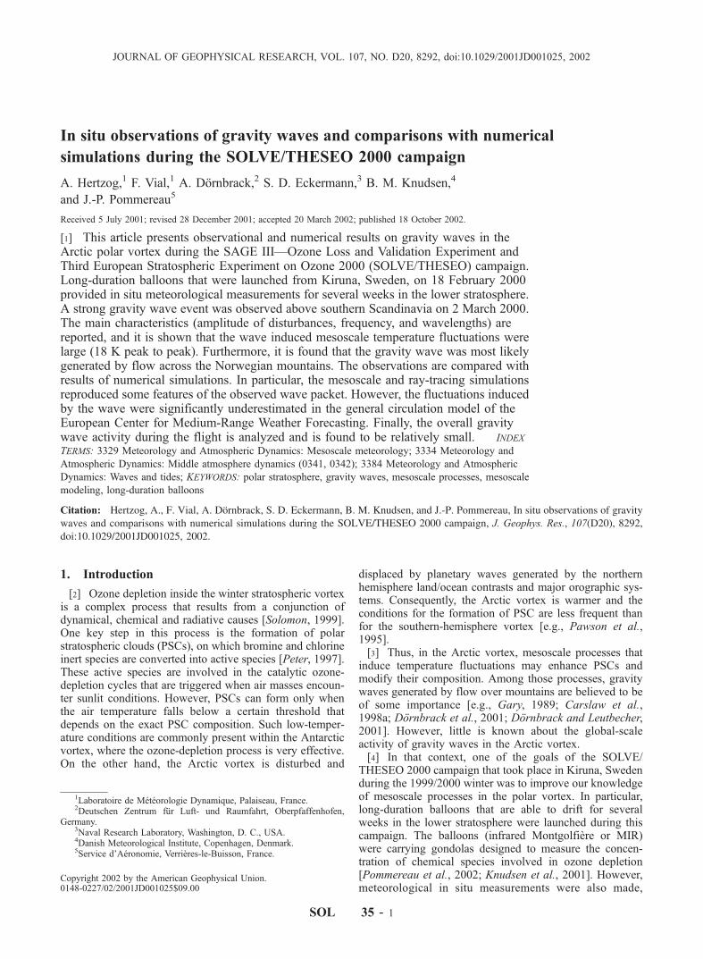
vortex. Its trajectory is shown in Figure 1. The MIR madefour revolutions in the vortex and flew both above mountainranges (e.g., Scandinavia, Urals, Greenland, Spitzbergen)and above flat areas (e.g., ocean, ice-pack, western Siberia).[9] The altitude of the MIR is controlled by the temper-

ature of the air inside the balloon, which is heated by theballoon envelope. The envelope absorbs the solar fluxduring the day and the telluric infrared flux at night.Consequently, the MIR altitude is higher during the daythan at night and the MIR exhibits vertical excursions atsunrise and sunset.

[10] The MIR carried two gondolas: Salsa, a gondolahosting several instruments measuring stratospheric minorspecies (a SAOZ-UV visible spectrometer, a tunable-diodelaser to measure CH4 and a Lyman a hygrometer) andSamba, the French Space Agency (CNES) gondola, thatwas responsible for meteorological measurements and forthe flight security. In this paper, we will focus on analysis ofthe purely dynamical measurements. Pommereau et al.[2002] and Vial et al. [2001] reported on the accuracy ofthe various meteorological sensors: Briefly, the wind veloc-ity is deduced from successive GPS 3-D positions and theaccuracy is better than 0.3 m s�1; successive pressuremeasurements are obtained with a 0.1 hPa precision (thepressure accuracy is known to about 1 hPa), and temper-ature measurements are made during night and sunset withan accuracy of 0.5 K (during daylight hours, the temperaturesensors are perturbed by solar radiation and by heat emittedfrom the gondola and will not be used in this study).Measurements were obtained every 10 min along the flighttrack. Some GPS points were not correctly recorded duringvertical-excursion phases, resulting in some missing wind-velocity measurements at sunrise and sunset.[11] The ability of long-duration balloons to track strato-

spheric perturbations due to gravity waves was demonstratedby Massman [1978, 1981], Vial et al. [2001], and Hertzogand Vial [2001]. These authors showed that the Lagrangiandata they provide could be analyzed to provide directmeasurements of the intrinsic frequencies of gravity waves,as well as other wave quantities. Intrinsic frequencies cannotbe measured directly from ground-based or airborne instru-ments [e.g., Fritts and VanZandt, 1987; Vincent and Eck-ermann, 1990; Bacmeister et al., 1996], and so this importantwave parameter can only be inferred using more indirect dataanalysis methods [e.g.,Hirota and Niki, 1985;Cot and Barat,

Figure 1. Trajectory of the second MIR. The MIR waslaunched from Kiruna, Sweden on 18 February 2000 andwas destroyed over Belarus on 8 March 2000 after 18 daysof flight. Daytime sections of the flight are dashed.

SOL 35 - 2 HERTZOG ET AL.: IN SITU OBSERVATIONS OF GRAVITY WAVES

1986; Eckermann, 1996; Dean-Day et al., 1998] which canbe subject to various interpretative uncertainties [e.g., Eck-ermann and Hocking, 1989; Hines, 1989]. Thus we have nodirect measurements of gravity wave intrinsic frequencies,which are essential to assess, for instance, wave inducedcooling rates [Bacmeister et al., 1999].

2.2. Models

2.2.1. MM5[12] Simulations are performed using the MM5 three-

dimensional nonhydrostatic mesoscale model [Dudhia,1993; Grell et al., 1994]. The outer model domain iscentered around 10�E, 60�N with an extension of 2208 km� 2208 km. In this domain, the horizontal grid size is 24km. A local grid refinement scheme with a horizontal gridsize of 8 km is applied south of the Scandinavianpeninsula to resolve most of the horizontal wave numberspectrum of vertically propagating gravity waves excitedby mountains. The model extends up to 30 km, whereradiative boundary conditions avoid spurious verticalreflection of waves. Simulated fields are stored everytwo hours.2.2.2. ECMWF[13] We will also compare our observations with general

circulation simulations performed with the European Centerfor Medium-Range Weather Forecasting (ECMWF) model.The version used in this study is the T319 spherical-harmonic model. The simulated fields are extracted on a0.4�latitude-longitude grid. The model has 60 levels in thevertical, up to 0.1 hPa and it assimilates the AdvancedMicrowave Sounding Unit data. To that purpose, a four-dimensional variational data assimilation scheme is used[Rabier et al., 2000]. The analyses are available every 6hours. To deal with the gravity wave drag forced by subgridscale mountains the scheme by Lott and Miller [1997] isused. The model mountains are based on the GTOPO30

data at 3000 � 3000 resolution, but scales below about 5 kmdo not contribute.2.2.3. Mountain Wave Forecast Model (MWFM)[14] The model used here (MWFM 2.0) is a ray-based

extension of the initial model developed by Bacmeister etal. [1994], which models mountain waves based on quasi-two dimensional fits to dominant ridge-like structures inEarth’s topography. MWFM 2.0 incorporates a number ofchanges from the MWFM 1.0 model. Most importantly, itreplaces the two-dimensional irrotational hydrostatic gravitywave model used in MWFM 1.0 with ray-tracing equationsgoverned by a rotating nonhydrostatic dispersion relation.Wave amplitudes are governed by conservation of verticalflux of wave action density, and wave breaking thresholdsdue to dynamical and convective instabilities are parame-terized. Peak temperature and horizontal velocity ampli-tudes are calculated from the wave action densities usingstandard polarization relations. The formulation is similar tothat from Marks and Eckermann [1995]. Temporal andhorizontal variations of the background atmosphere areignored, so that ground-based wave phase speeds remainstationary. Three dimensionality in mountain wave patternsis also accommodated by launching waves at differentazimuths, with maximum amplitudes perpendicular to thequasi-two-dimensional ridge axis and amplitude scaled fromthere, according to the three-dimensionality of the analyzedridge feature. Thus MWFM 2.0 can parameterize importantmountain wave effects that the old model could not, such asvertical reflection [e.g., Schoeberl, 1985], three-dimensional‘‘ship wave’’ patterns [Broutman et al., 2001] and down-stream dispersion due to nonhydrostatic or near-inertial

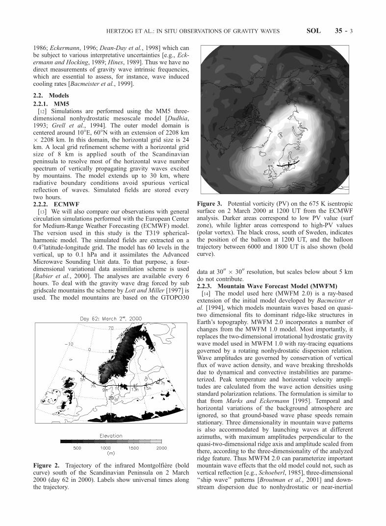
Figure 2. Trajectory of the infrared Montgolfiere (boldcurve) south of the Scandinavian Peninsula on 2 March2000 (day 62 in 2000). Labels show universal times alongthe trajectory.

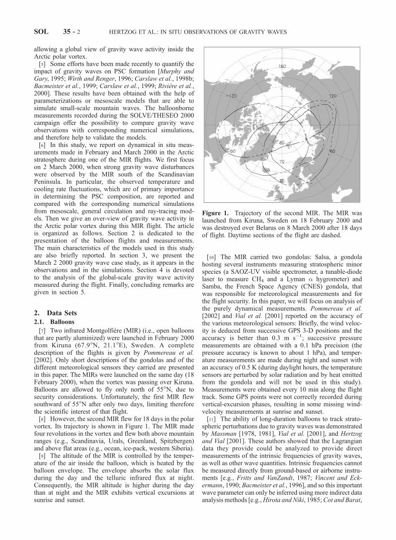
Figure 3. Potential vorticity (PV) on the 675 K isentropicsurface on 2 March 2000 at 1200 UT from the ECMWFanalysis. Darker areas correspond to low PV value (surfzone), while lighter areas correspond to high-PV values(polar vortex). The black cross, south of Sweden, indicatesthe position of the balloon at 1200 UT, and the balloontrajectory between 6000 and 1800 UT is also shown (boldcurve).

HERTZOG ET AL.: IN SITU OBSERVATIONS OF GRAVITY WAVES SOL 35 - 3

effects. Both the 1.0 and 2.0 models (as well as MM5) wereused in forecast mode throughout SOLVE/THESEO 2000.[15] MWFM is a numerical mountain wave parameter-

ization, unlike ECMWF and MM5 that model the entireatmospheric flow using the primitive equations, includingany explicitly-resolved mountain waves. Additionally,MWFM focuses mostly on topographic features that areunresolved by most global models (i.e., sub gridscale), andthus typically simulates small-to-medium scale gravitywaves with horizontal wavelengths in the 10–200 km range.

3. Case Study

3.1. Observations

[16] The event studied in this section occurred on 2 March2000. At that time, the MIR was flying south of theNorwegian coast (see Figure 2) along the inner side of themain potential vorticity gradient (Figure 3). Note that it didnot pass over the Norwegian mountains but flew until 1100UT over the sea.[17] Figure 4 shows the MIR altitude, pressure and

velocities on this day. At approximately 0600 UT, the

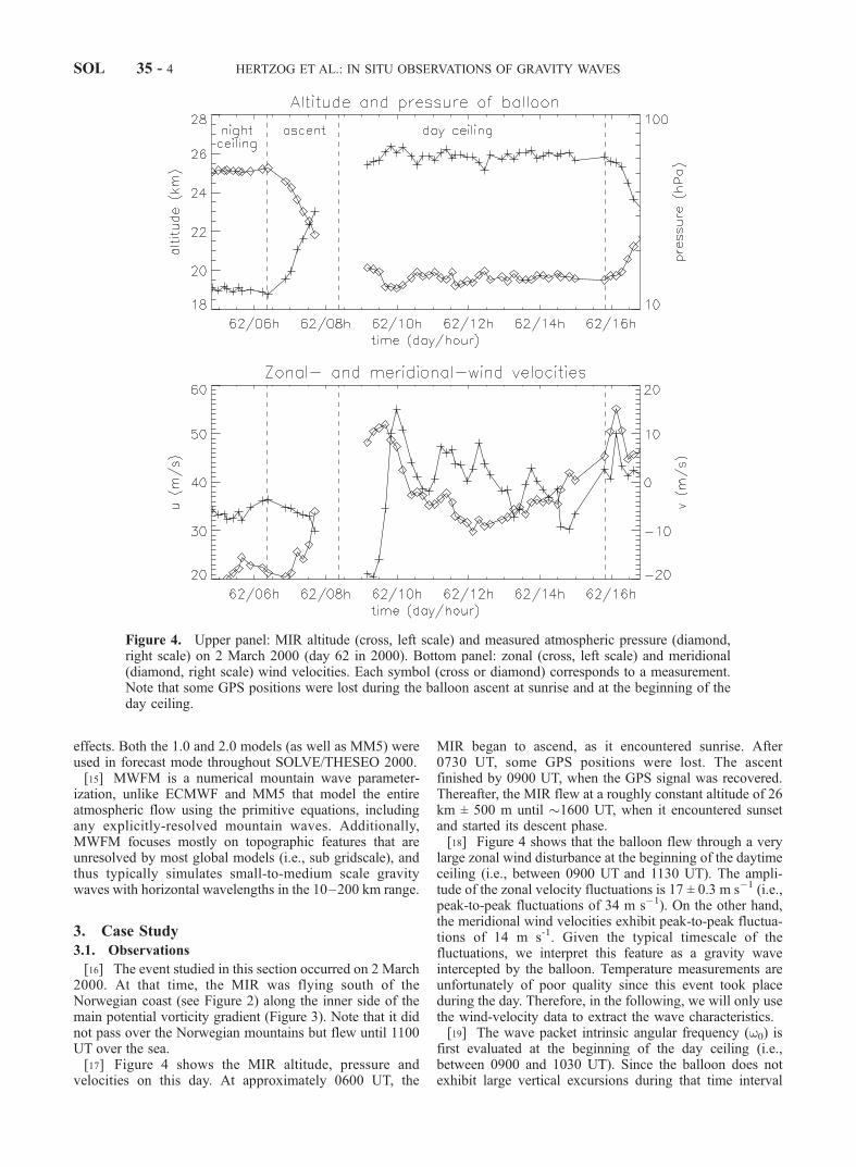
MIR began to ascend, as it encountered sunrise. After0730 UT, some GPS positions were lost. The ascentfinished by 0900 UT, when the GPS signal was recovered.Thereafter, the MIR flew at a roughly constant altitude of 26km ± 500 m until �1600 UT, when it encountered sunsetand started its descent phase.[18] Figure 4 shows that the balloon flew through a very

large zonal wind disturbance at the beginning of the daytimeceiling (i.e., between 0900 UT and 1130 UT). The ampli-tude of the zonal velocity fluctuations is 17 ± 0.3 m s�1 (i.e.,peak-to-peak fluctuations of 34 m s�1). On the other hand,the meridional wind velocities exhibit peak-to-peak fluctua-tions of 14 m s-1. Given the typical timescale of thefluctuations, we interpret this feature as a gravity waveintercepted by the balloon. Temperature measurements areunfortunately of poor quality since this event took placeduring the day. Therefore, in the following, we will only usethe wind-velocity data to extract the wave characteristics.[19] The wave packet intrinsic angular frequency (w0) is

first evaluated at the beginning of the day ceiling (i.e.,between 0900 and 1030 UT). Since the balloon does notexhibit large vertical excursions during that time interval

Figure 4. Upper panel: MIR altitude (cross, left scale) and measured atmospheric pressure (diamond,right scale) on 2 March 2000 (day 62 in 2000). Bottom panel: zonal (cross, left scale) and meridional(diamond, right scale) wind velocities. Each symbol (cross or diamond) corresponds to a measurement.Note that some GPS positions were lost during the balloon ascent at sunrise and at the beginning of theday ceiling.

SOL 35 - 4 HERTZOG ET AL.: IN SITU OBSERVATIONS OF GRAVITY WAVES

and is moreover advected by the mean wind, the period ofthe observed zonal wind fluctuations measured on board theballoon is the intrinsic period of the wave packet (i.e., theperiod relative to the mean flow). We obtain: 2p/w0 � 75 ±5 min. Another estimate of the wave intrinsic period can beobtained by the analysis of the horizontal velocity hodo-graph: The ratio between the ellipse long and short axes is

equal to w0/f, where f is the inertial period [Andrews et al.,1987]. In our case, this analysis (not shown) yields 2p/w0 �85 ± 1 min. We will therefore assume in the following thatthe intrinsic period of the wave packet is 80 ± 7 min.[20] The inertial period (2p/f ) at the balloon latitude

(�58�) is �14 h, while the Brunt-Vaisala frequency (N )estimated in the mesoscale MM5 simulations is 2.5 10�2 ±

Table 1. Observed and Simulated Wave Packet Characteristics

IntrinsicPeriod, min

Wavelengths Direction ofPropagationa u0, m s�1 T0, K

Maximum CoolingRate, K h�1Horizontal, km Vertical, km

Observations 80 ± 7 202b ± 21 10.5c ± 1.5 173� ± 1� 17 ± 0.3 9.1d ± 1.5 �43d ± 11MM5 105 200 8 169� 17 11 �38

ECMWF 160 350 9 180� 3 1.5 �3.5MWFM 90 200 10 165� 19 8 �33aAngles are counted positively anticlockwise, and 0� corresponds to eastward propagation relative to the ground.bObtained by assuming that the wave is stationary relative to the ground.cAs in noteb, and applying the dispersion relationship for gravity waves.dObtained by applying the polarization relationships for gravity waves.

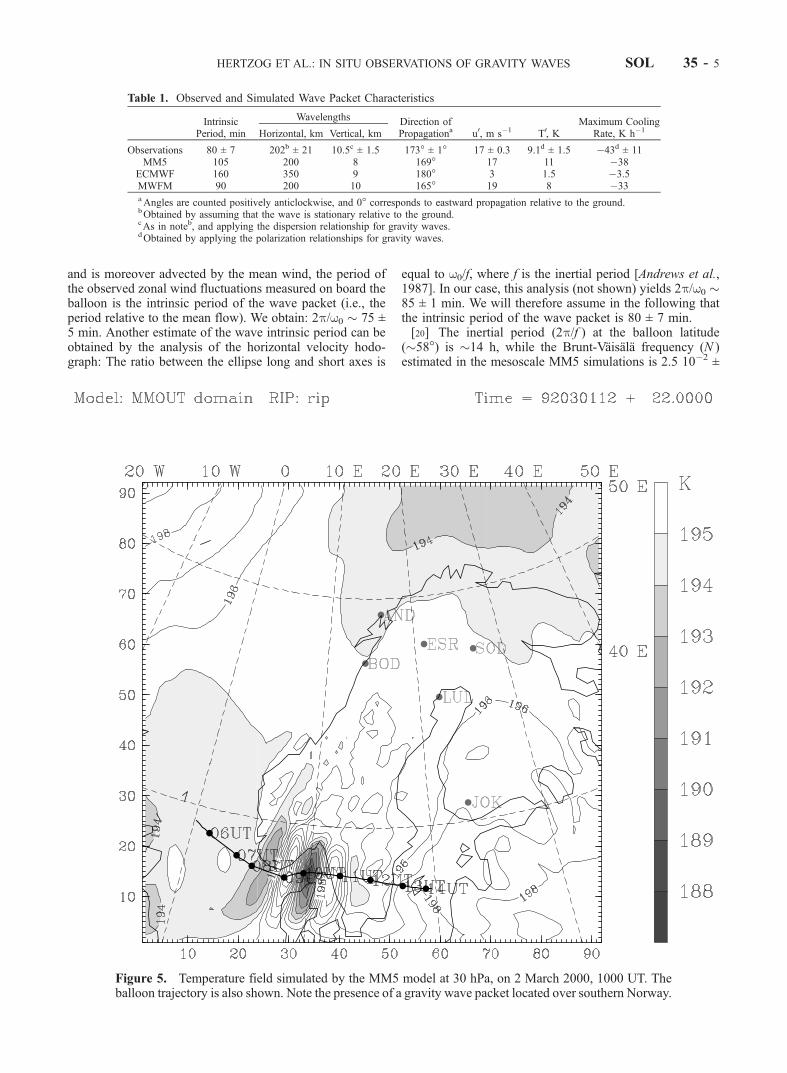
Figure 5. Temperature field simulated by the MM5 model at 30 hPa, on 2 March 2000, 1000 UT. Theballoon trajectory is also shown. Note the presence of a gravity wave packet located over southern Norway.

HERTZOG ET AL.: IN SITU OBSERVATIONS OF GRAVITY WAVES SOL 35 - 5

0.3 10�2 rad s�1 in the lower stratosphere (corresponding toa period 4 min). Therefore we can apply the so-calledmidfrequency approximation.

j f j � jw0j � N : ð1Þ

[21] Since the amplitude of the zonal velocity fluctuationsis much larger than that of the meridional velocity fluctua-tions, the wave vector is almost zonally oriented. Indeed,the long axis of the hodograph, which is parallel to the wavevector, is oriented 7� off the zonal direction, either north ofdue west or south of due east. The wind-velocity fluctua-tions (u0) are thus linked to the amplitude of the temperaturedisturbance (T 0) by the polarization relationship [Andrews etal., 1987]:

T 0 ¼ T0N

gu0; ð2Þ

where T0 is the background temperature, which wasestimated from the measurements made during sunset(i.e., at the same altitude as the daytime ceiling but in theabsence of solar radiation) to be 210 ± 4.5 K. Hence weobtain: T 0 = 9.1 ± 1.5 K (i.e., peak-to-peak fluctuations of�18 K). Finally, the maximum (reversible) cooling rateinduced by the wave (T 0

t ) can be computed as:

T 0t ¼ �w0T

0 ¼ �43 11K h�1: ð3Þ

[22] To get more insights into the characteristics of thewave packet, we will now assume that it was generated over

the Norwegian mountains by a quasi-stationary flow. Thisassumption will be discussed later on. In this context, thewave packet is stationary relative to the ground, so that itsintrinsic angular frequency is given by [Andrews et al.,1987]:

w0 ¼ �~kh:~u; ð4Þ

where~kh = (k, l ) is the horizontal wave vector, and~u = (u, v)the horizontal wind vector. In our case, this equationreduces to:

w0 ¼ �ku; ð5Þ

where u � 42 m s�1. This yields a horizontal wavelength(2p/|k|) of 202 ± 21 km. Note that k is negative here, inorder for the wave to be stationary relative to the ground,and consequently the wave vector is aligned 7� north of duewest. Finally, the vertical wave number (m) is computedusing the simplified midfrequency dispersion relationshipfor gravity waves:

m ¼ N

w0

k ¼ �N

u; ð6Þ

where we have assumed that the wave packet propagatesupward (m and w0 have opposite signs). It yields a verticalwavelength (2p/|m|) of 10.5 ± 1.5 km. This verticalwavelength is relatively large: Classical spectra showhighest values of energy density at about 2p/m

*= 2–4

Figure 6. Cross section of the zonal wind velocity on 2 March 2000, 1000 UT, in the MM5 model. Thecross section coincides with the balloon trajectory south of Norway. The balloon altitude as a function oftime is shown by the solid black line. Stars are plotted every 2 h.

SOL 35 - 6 HERTZOG ET AL.: IN SITU OBSERVATIONS OF GRAVITY WAVES

km in the lower stratosphere [e.g., Allen and Vincent, 1995].However, we have to stress that this long wavelength isneeded to prevent static (and even dynamic) instabilitiesfrom developing, given the amplitude of the temperaturefluctuations [see, e.g., Eckermann and Preusse, 1999]. Forinstance, the minimum value reached by temperaturevertical gradients induced by the wave packet is mT 0 ��5.5 K km�1, which does not exceed the dry adiabaticlapse rate (�10 K km�1). On the other hand, the wavepacket vertical wavelength is not so large that the factor 1/4H2 needs to be included in (6), where H is the density scaleheight of the atmosphere. Indeed, we can consider that |m|� 1/2H, with H � 6 km in the lower stratosphere.[23] All the characteristics of the observed wave packet

are reported in Table 1. In the following section, we analyzethe wave packet as it is simulated in different dynamicalmodels and compare the simulated characteristics with theobserved ones.

3.2. Simulations

3.2.1. MM5[24] The simulated temperature field at 30 hPa produced

by the MM5 model, on 2 March 2000, 1000 UT is shownon Figure 5. The model obviously succeeded in producing agravity wave packet at the geographical location where andtime when the balloon was flying south of Norway. (Note,however, that the balloon was flying 2 km higher.) Two anda half wavelengths are clearly visible. In the model, thedisturbances of the background fields induced by the wave

packet maximize at 1000 UT (Figure 5). In the balloon data,the maximum amplitude was also observed at that time.This correspondence supports an interpretation of the simu-lated and the observed gravity wave as being the same eventand that it is therefore meaningful to compare the character-istics of both waves.[25] The zonal wind field simulated by the MM5 model at

1000 UT, as a function of longitude and altitude and on across section that coincides with the balloon trajectory southof the Scandinavian peninsula, is shown in Figure 6.[26] The wave packet appears in this figure as tilted

isocontours, east of 5�E and above 10 km. The amplitudeof the disturbances is increasing with altitude up to �27 km.Indeed, a strong numerical damping is imposed in theuppermost layers of the model, in order to avoid reflectionof waves at the top of the simulation. This damping preventsvertical propagationof the wave packet beyond 27 km. Notethat the tilt of isocontours is consistent with a gravity wavepropagating upward and westward relative to the wind, i.e.,the vertical phase speed of the wave is negative, while itsvertical group velocity is positive.[27] The balloon trajectory encounters the simulated

gravity wave packet at 0800 UT, i.e., at the time whenGPS points were lost (see Figure 4). The center of the wavepacket is reached at 1000 UT, as in the observations. Thecharacteristics of the simulated wave packet are alsoreported in Table 1. The amplitude of the zonal velocityfluctuations, the horizontal wavelength and the propagationdirection are well reproduced by the model. On the other

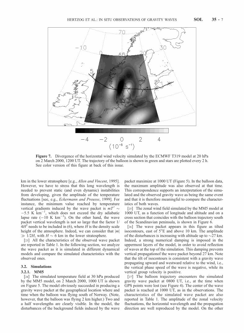
Figure 7. Divergence of the horizontal wind velocity simulated by the ECMWF T319 model at 20 hPaon 2 March 2000, 1200 UT. The trajectory of the balloon is shown in green and stars are plotted every 2 h.See color version of this figure at back of this issue.

HERTZOG ET AL.: IN SITU OBSERVATIONS OF GRAVITY WAVES SOL 35 - 7

hand, the period of the wave is 15 min longer in themodel,whereas the vertical wavelength is shorter and the amplitudeof the temperature fluctuations are overestimated by �2 K.[28] In conclusion, the simulated location, time, and char-

acteristics of the wave packet are in fair agreement with theobservations. The discrepancies that are observed could be atleast partly due to the limited resolution of the model, thefriction that is applied and the presence of the top boundaryclose to the wavepacket [Leutbecher and Volkert, 2000].3.2.2. ECMWF[29] The divergence of the horizontal wind at 20 hPa

simulated by the ECMWF T319 model on 2 March 2000,1200 UT is shown on Figure 7. This field easily enables usto identify gravity wave packets in general circulationmodels [e.g., O’Sullivan and Dunkerton, 1995; Moldovanet al., 2002]. In our case the gravity wave, through whichthe MIR flew south of Norway, is also captured by theECMWF simulation. Furthermore, the phase structure and

the geographical localization of the wave packet comparewell with the MM5 simulations (see Figure 5).[30] The wave packet characteristics in the ECMWF

simulation are reported in Table 1. The vertical wavelengthand the propagation direction agree fairly well with theobservations. However, several differences between thesimulation and the observations are obvious. In particular,the horizontal wavelengths and the period of the wave packetare overestimated by a factor of 2 in the ECMWF simulation.[31] The main discrepancy is in the amplitudes of the

disturbances, which are much lower in the ECMWF fieldsthan observed in the MIR data. First, it should be noticedthat the vertical resolution of the model is relatively coarsein the stratosphere (around 1 km at 25 km), so that gravitywaves may be poorly simulated even though the horizontaland temporal resolutions are high enough. For the caseconsidered however, the vertical wavelength of the wavepacket is much larger than1 km so that the this effect is

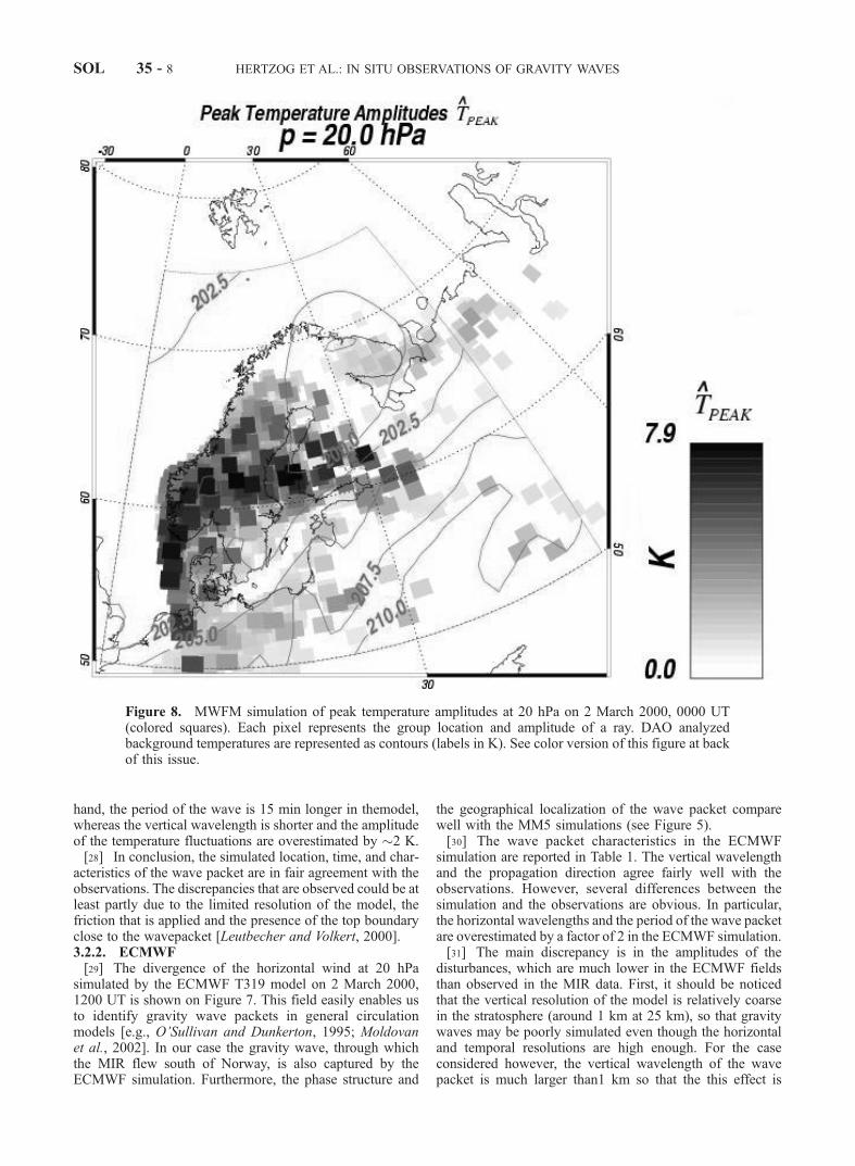
Figure 8. MWFM simulation of peak temperature amplitudes at 20 hPa on 2 March 2000, 0000 UT(colored squares). Each pixel represents the group location and amplitude of a ray. DAO analyzedbackground temperatures are represented as contours (labels in K). See color version of this figure at backof this issue.

SOL 35 - 8 HERTZOG ET AL.: IN SITU OBSERVATIONS OF GRAVITY WAVES

expected to be small. The most likely explanation is that afiltering is applied in the model to exclude the disturbancesthat induce strong divergence. This is done in order to avoidspurious energy transfer toward the smallest simulatedscales, which may cause the model to diverge. Conse-quently, disturbances induced by gravity waves may beseverely damped.3.2.3. MWFM[32] Figures 8 and 9 show hindcasts of peak amplitudes of

temperature (TPEAK) and total horizontal velocity (UPEAK),based on ‘‘late look’’ analysis winds and temperatures for 2March 2000 at 0000 UT from NASA’s Data AssimilationOffice (DAO) [Coy and Swinbank, 1997]. Fifty-four rayswere launched from each ridge feature: 3 individual hori-zontal wavelengths each launched at 18 equally spacedazimuths. Total horizontal wave numbers were calculated as

kh ¼ 1:5 J=�h; ð7Þ

where �h is the width of the short axis of the ridge feature,and J = 1, 2, 3: These assignments are tunable but are close

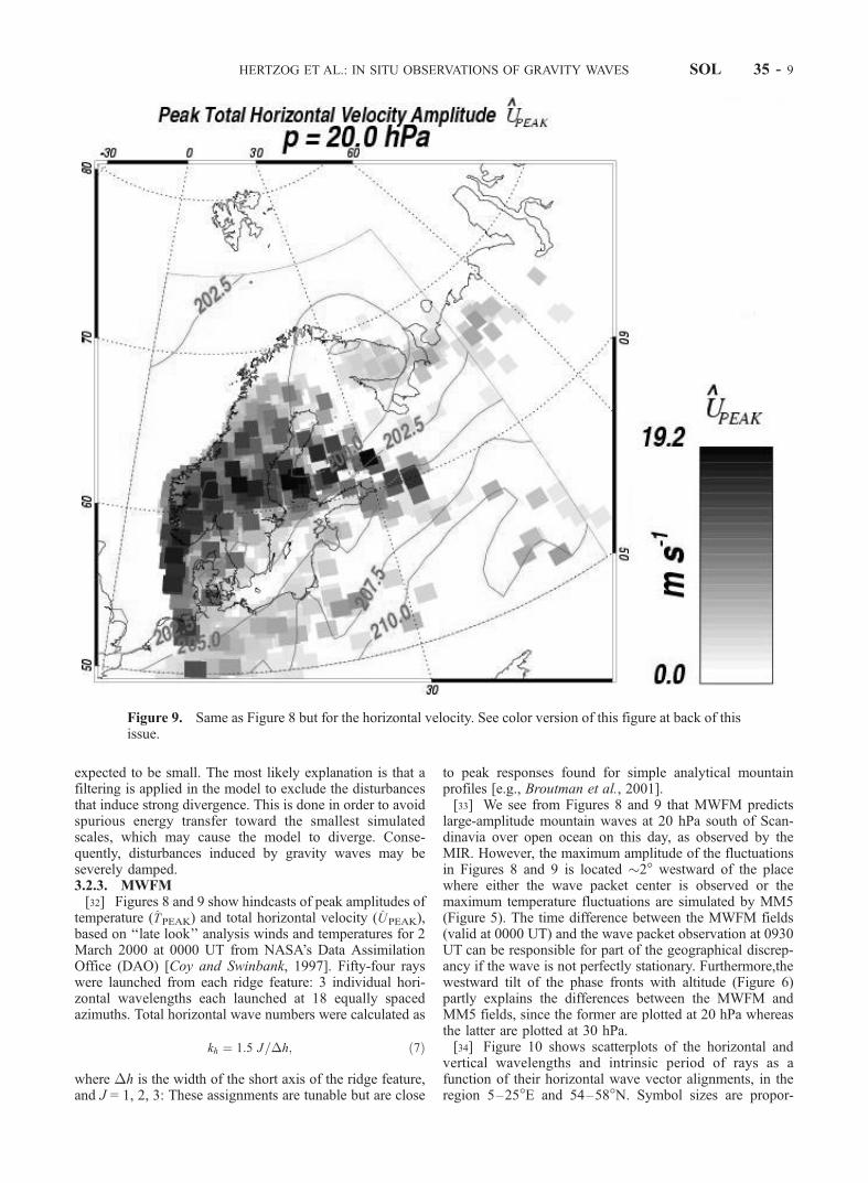
to peak responses found for simple analytical mountainprofiles [e.g., Broutman et al., 2001].[33] We see from Figures 8 and 9 that MWFM predicts

large-amplitude mountain waves at 20 hPa south of Scan-dinavia over open ocean on this day, as observed by theMIR. However, the maximum amplitude of the fluctuationsin Figures 8 and 9 is located �2� westward of the placewhere either the wave packet center is observed or themaximum temperature fluctuations are simulated by MM5(Figure 5). The time difference between the MWFM fields(valid at 0000 UT) and the wave packet observation at 0930UT can be responsible for part of the geographical discrep-ancy if the wave is not perfectly stationary. Furthermore,thewestward tilt of the phase fronts with altitude (Figure 6)partly explains the differences between the MWFM andMM5 fields, since the former are plotted at 20 hPa whereasthe latter are plotted at 30 hPa.[34] Figure 10 shows scatterplots of the horizontal and

vertical wavelengths and intrinsic period of rays as afunction of their horizontal wave vector alignments, in theregion 5–25�E and 54–58�N. Symbol sizes are propor-

Figure 9. Same as Figure 8 but for the horizontal velocity. See color version of this figure at back of thisissue.

HERTZOG ET AL.: IN SITU OBSERVATIONS OF GRAVITY WAVES SOL 35 - 9

tional to TPEAK2 for each ray. The largest amplitude moun-

tain wave rays are aligned �10–20� south of due east. Thepeak wavelengths and periods are similar to those observed,as summarized in Table 1.

3.3. Discussion

[35] In this section, we look more carefully on the mech-anism that generated the wave packet observed by the bal-loon. To do this, we use the ECMWF T319 simulation. It hasbeen assumed in section 3.1 that the gravity-packet wasgenerated by the interaction between the Norwegian moun-tains and the flow close to the ground. First, it should benoted that the Norwegian mountains are a significant oro-graphic system (the highest peak is located in the southernpart of the system and has an altitude greater than 2000 m

ASL). Furthermore, on 2 March 2000, 0000 UT, the low-level wind was blowing from the northwest on the westernside of the mountains, i.e., perpendicular to the main ridgeaxis (not shown). At 700 hPa, the wind speed reached valuesof�20 m s�1, so that favorable conditions for the generationof mountain waves were present.[36] To be observed by the balloon, the wave packet had to

propagate upward from the troposphere to the stratosphere. Inorder to follow this propagation, longitude-altitude crosssections at 59�N of the divergence of the ECMWF horizontalvelocity on 2 March 2000 are shown in Figure 11. The wavepacket propagates from the ground (between 5�E and 10�E,i.e., southern Norway) at 0000 UT to the stratosphere at 1200UT, where it is observed by the MIR.

Figure 10. Scatterplots of horizontal wavelengths (upperpanel), vertical wavelengths (middle panel), and intrinsicperiods (lower panel) of rays simulated by the MWFMmodel above southern Scandinavia. The size of the symbolsis proportional to the square of the temperature fluctuationsassociated with each ray.

Figure 11. Divergence of the horizontal wind velocitysimulated by the ECMWF T319 model at 59�N, on 2 March2000, 0000 UT (top), 0600 UT (middle), and 1200 UT(bottom). Contours are plotted every 2 � 10�5 s�1, andcontours associated with negative values are dashed.

SOL 35 - 10 HERTZOG ET AL.: IN SITU OBSERVATIONS OF GRAVITY WAVES

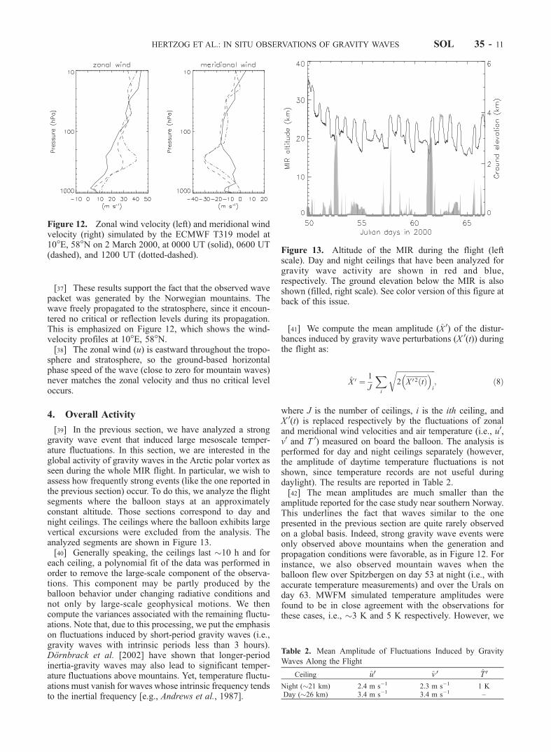
[37] These results support the fact that the observed wavepacket was generated by the Norwegian mountains. Thewave freely propagated to the stratosphere, since it encoun-tered no critical or reflection levels during its propagation.This is emphasized on Figure 12, which shows the wind-velocity profiles at 10�E, 58�N.[38] The zonal wind (u) is eastward throughout the tropo-

sphere and stratosphere, so the ground-based horizontalphase speed of the wave (close to zero for mountain waves)never matches the zonal velocity and thus no critical leveloccurs.

4. Overall Activity

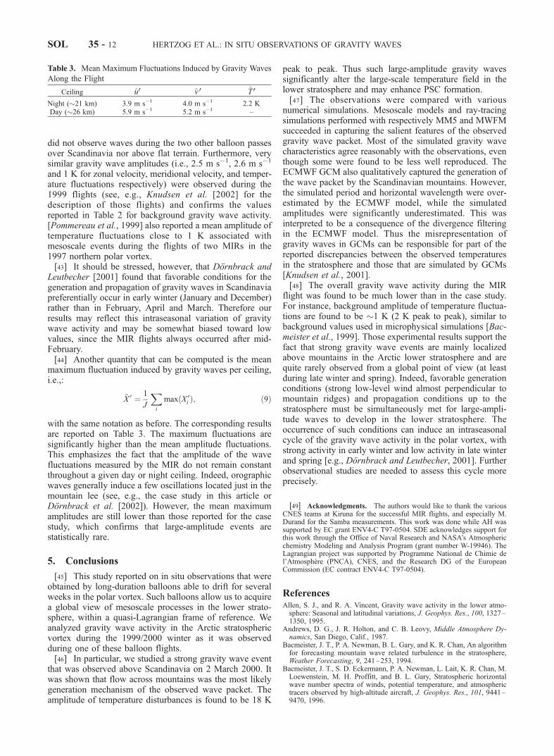
[39] In the previous section, we have analyzed a stronggravity wave event that induced large mesoscale temper-ature fluctuations. In this section, we are interested in theglobal activity of gravity waves in the Arctic polar vortex asseen during the whole MIR flight. In particular, we wish toassess how frequently strong events (like the one reported inthe previous section) occur. To do this, we analyze the flightsegments where the balloon stays at an approximatelyconstant altitude. Those sections correspond to day andnight ceilings. The ceilings where the balloon exhibits largevertical excursions were excluded from the analysis. Theanalyzed segments are shown in Figure 13.[40] Generally speaking, the ceilings last �10 h and for

each ceiling, a polynomial fit of the data was performed inorder to remove the large-scale component of the observa-tions. This component may be partly produced by theballoon behavior under changing radiative conditions andnot only by large-scale geophysical motions. We thencompute the variances associated with the remaining fluctu-ations. Note that, due to this processing, we put the emphasison fluctuations induced by short-period gravity waves (i.e.,gravity waves with intrinsic periods less than 3 hours).Dornbrack et al. [2002] have shown that longer-periodinertia-gravity waves may also lead to significant temper-ature fluctuations above mountains. Yet, temperature fluctu-ations must vanish for waves whose intrinsic frequency tendsto the inertial frequency [e.g., Andrews et al., 1987].

[41] We compute the mean amplitude (X 0) of the distur-bances induced by gravity wave perturbations (X 0(t)) duringthe flight as:

X 0 ¼ 1

J

Xi

ffiffiffiffiffiffiffiffiffiffiffiffiffiffiffiffiffiffiffiffiffiffi2 X 0 2ðtÞ� �

i

r; ð8Þ

where J is the number of ceilings, i is the ith ceiling, andX 0(t) is replaced respectively by the fluctuations of zonaland meridional wind velocities and air temperature (i.e., u0,v0 and T 0) measured on board the balloon. The analysis isperformed for day and night ceilings separately (however,the amplitude of daytime temperature fluctuations is notshown, since temperature records are not useful duringdaylight). The results are reported in Table 2.[42] The mean amplitudes are much smaller than the

amplitude reported for the case study near southern Norway.This underlines the fact that waves similar to the onepresented in the previous section are quite rarely observedon a global basis. Indeed, strong gravity wave events wereonly observed above mountains when the generation andpropagation conditions were favorable, as in Figure 12. Forinstance, we also observed mountain waves when theballoon flew over Spitzbergen on day 53 at night (i.e., withaccurate temperature measurements) and over the Urals onday 63. MWFM simulated temperature amplitudes werefound to be in close agreement with the observations forthese cases, i.e., �3 K and 5 K respectively. However, we

Figure 12. Zonal wind velocity (left) and meridional windvelocity (right) simulated by the ECMWF T319 model at10�E, 58�N on 2 March 2000, at 0000 UT (solid), 0600 UT(dashed), and 1200 UT (dotted-dashed).

Figure 13. Altitude of the MIR during the flight (leftscale). Day and night ceilings that have been analyzed forgravity wave activity are shown in red and blue,respectively. The ground elevation below the MIR is alsoshown (filled, right scale). See color version of this figure atback of this issue.

Table 2. Mean Amplitude of Fluctuations Induced by Gravity

Waves Along the Flight

Ceiling u0 v 0 T 0

Night (�21 km) 2.4 m s�1 2.3 m s�1 1 KDay (�26 km) 3.4 m s�1 3.4 m s�1 –

HERTZOG ET AL.: IN SITU OBSERVATIONS OF GRAVITY WAVES SOL 35 - 11

did not observe waves during the two other balloon passesover Scandinavia nor above flat terrain. Furthermore, verysimilar gravity wave amplitudes (i.e., 2.5 m s�1, 2.6 m s�1

and 1 K for zonal velocity, meridional velocity, and temper-ature fluctuations respectively) were observed during the1999 flights (see, e.g., Knudsen et al. [2002] for thedescription of those flights) and confirms the valuesreported in Table 2 for background gravity wave activity.[Pommereau et al., 1999] also reported a mean amplitude oftemperature fluctuations close to 1 K associated withmesoscale events during the flights of two MIRs in the1997 northern polar vortex.[43] It should be stressed, however, that Dornbrack and

Leutbecher [2001] found that favorable conditions for thegeneration and propagation of gravity waves in Scandinaviapreferentially occur in early winter (January and December)rather than in February, April and March. Therefore ourresults may reflect this intraseasonal variation of gravitywave activity and may be somewhat biased toward lowvalues, since the MIR flights always occurred after mid-February.[44] Another quantity that can be computed is the mean

maximum fluctuation induced by gravity waves per ceiling,i.e.,:

~X 0 ¼ 1

J

Xi

maxðX 0i Þ; ð9Þ

with the same notation as before. The corresponding resultsare reported on Table 3. The maximum fluctuations aresignificantly higher than the mean amplitude fluctuations.This emphasizes the fact that the amplitude of the wavefluctuations measured by the MIR do not remain constantthroughout a given day or night ceiling. Indeed, orographicwaves generally induce a few oscillations located just in themountain lee (see, e.g., the case study in this article orDornbrack et al. [2002]). However, the mean maximumamplitudes are still lower than those reported for the casestudy, which confirms that large-amplitude events arestatistically rare.

5. Conclusions

[45] This study reported on in situ observations that wereobtained by long-duration balloons able to drift for severalweeks in the polar vortex. Such balloons allow us to acquirea global view of mesoscale processes in the lower strato-sphere, within a quasi-Lagrangian frame of reference. Weanalyzed gravity wave activity in the Arctic stratosphericvortex during the 1999/2000 winter as it was observedduring one of these balloon flights.[46] In particular, we studied a strong gravity wave event

that was observed above Scandinavia on 2 March 2000. Itwas shown that flow across mountains was the most likelygeneration mechanism of the observed wave packet. Theamplitude of temperature disturbances is found to be 18 K

peak to peak. Thus such large-amplitude gravity wavessignificantly alter the large-scale temperature field in thelower stratosphere and may enhance PSC formation.[47] The observations were compared with various

numerical simulations. Mesoscale models and ray-tracingsimulations performed with respectively MM5 and MWFMsucceeded in capturing the salient features of the observedgravity wave packet. Most of the simulated gravity wavecharacteristics agree reasonably with the observations, eventhough some were found to be less well reproduced. TheECMWF GCM also qualitatively captured the generation ofthe wave packet by the Scandinavian mountains. However,the simulated period and horizontal wavelength were over-estimated by the ECMWF model, while the simulatedamplitudes were significantly underestimated. This wasinterpreted to be a consequence of the divergence filteringin the ECMWF model. Thus the misrepresentation ofgravity waves in GCMs can be responsible for part of thereported discrepancies between the observed temperaturesin the stratosphere and those that are simulated by GCMs[Knudsen et al., 2001].[48] The overall gravity wave activity during the MIR

flight was found to be much lower than in the case study.For instance, background amplitude of temperature fluctua-tions are found to be �1 K (2 K peak to peak), similar tobackground values used in microphysical simulations [Bac-meister et al., 1999]. Those experimental results support thefact that strong gravity wave events are mainly localizedabove mountains in the Arctic lower stratosphere and arequite rarely observed from a global point of view (at leastduring late winter and spring). Indeed, favorable generationconditions (strong low-level wind almost perpendicular tomountain ridges) and propagation conditions up to thestratosphere must be simultaneously met for large-ampli-tude waves to develop in the lower stratosphere. Theoccurrence of such conditions can induce an intraseasonalcycle of the gravity wave activity in the polar vortex, withstrong activity in early winter and low activity in late winterand spring [e.g., Dornbrack and Leutbecher, 2001]. Furtherobservational studies are needed to assess this cycle moreprecisely.

[49] Acknowledgments. The authors would like to thank the variousCNES teams at Kiruna for the successful MIR flights, and especially M.Durand for the Samba measurements. This work was done while AH wassupported by EC grant ENV4-C T97-0504. SDE acknowledges support forthis work through the Office of Naval Research and NASA’s Atmosphericchemistry Modeling and Analysis Program (grant number W-19946). TheLagrangian project was supported by Programme National de Chimie del’Atmosphere (PNCA), CNES, and the Research DG of the EuropeanCommission (EC contract ENV4-C T97-0504).

ReferencesAllen, S. J., and R. A. Vincent, Gravity wave activity in the lower atmo-sphere: Seasonal and latitudinal variations, J. Geophys. Res., 100, 1327–1350, 1995.

Andrews, D. G., J. R. Holton, and C. B. Leovy, Middle Atmosphere Dy-namics, San Diego, Calif., 1987.

Bacmeister, J. T., P. A. Newman, B. L. Gary, and K. R. Chan, An algorithmfor forecasting mountain wave related turbulence in the stratosphere,Weather Forecasting, 9, 241–253, 1994.

Bacmeister, J. T., S. D. Eckermann, P. A. Newman, L. Lait, K. R. Chan, M.Loewenstein, M. H. Proffitt, and B. L. Gary, Stratospheric horizontalwave number spectra of winds, potential temperature, and atmospherictracers observed by high-altitude aircraft, J. Geophys. Res., 101, 9441–9470, 1996.

Table 3. Mean Maximum Fluctuations Induced by Gravity Waves

Along the Flight

Ceiling u0 v 0 T 0

Night (�21 km) 3.9 m s�1 4.0 m s�1 2.2 KDay (�26 km) 5.9 m s�1 5.2 m s�1 –

SOL 35 - 12 HERTZOG ET AL.: IN SITU OBSERVATIONS OF GRAVITY WAVES

Bacmeister, J. T., S. D. Eckermann, A. Tsias, K. S. Carslaw, and T. Peter,Mesoscale temperature fluctuations induced by a spectrum of gravitywaves: A comparison of parameterizations and their impact on strato-spheric microphysics, J. Atmos., 56, 1913–1924, 1999.

Broutman, D., J. W. Rottman, and S. D. Eckermann, A hybrid method foranalyzing wave propagation from a localized source, with application tomountain waves, Q. J. R. Meteorol. Soc., 127, 129–146, 2001.

Carslaw, K. S., et al., Increased stratospheric ozone depletion due to moun-tain-induced atmospheric waves, Nature, 391, 675–678, 1998a.

Carslaw, K. S., et al., Particle microphysics and chemistry in remotelyobserved mountain polar stratospheric clouds, J. Geophys. Res., 103,5785–5796, 1998b.

Carslaw, K. S., T. Peter, J. T. Bacmeister, and S. D. Eckermann, Widespreadsolid particle formation by mountain waves in the Arctic stratosphere,J. Geophys. Res., 104, 1827–1836, 1999.

Cot, C., and J. Barat, wave turbulence interaction in the stratosphere: A casestudy, J. Geophys. Res., 91, 2749–2756, 1986.

Coy, L., and R. Swinbank, Characteristics of stratospheric winds and tem-peratures produced by data assimilation, J. Geophys. Res., 102, 25,763–25,781, 1997.

Dean-Day, J., K. R. Chan, S. W. Bowen, T. P. Bui, B. L. Gary, and M. J.Mahoney, Dynamics of Rocky Mountain lee waves observed duringSUCCESS, Geophys. Res. Lett., 25, 1351–1354, 1998.

Dornbrack, A., and M. Leutbecher, Relevance of mountain wave coolingfor the formation of polar stratospheric clouds over Scandinavia: A 20year climatology, J. Geophys. Res., 106, 1583–1593, 2001.

Dornbrack, A., M. Leutbecher, J. Reichardt, A. Behrendt, K. P. Muller, andG. Baumgarten, Relevance of mountain wave cooling for the formationof polar stratospheric clouds over Scandinavia: Mesoscale dynamics andobservations for January 1997, J. Geophys. Res., 106, 1569–1581, 2001.

Dornbrack, A., T. Birner, A. Fix, H. Flentje, A. Meister, H. Schmid, E. V.Browell, and M. J. Mahoney, Evidence for inertia gravity waves for-ming polar stratospheric clouds over Scandinavia, J. Geophys., 107,doi:10.1029/2001JD000452, in press, 2002.

Dudhia, J., A non-hydrostatic version of the Penn State-NCAR mesoscalemodel: Validation tests and simulation of an Atlantic cyclone and coldfront, Mon. Weather Rev., 121, 1493–1513, 1993.

Eckermann, S. D., Hodographic analysis of gravity waves: Relationshipsamong Stokes parameters, rotary spectra, and cross-spectral methods,J. Geophys., 101, 19,169–19,174, 1996.

Eckermann, S. D., and W. K. Hocking, Effect of superposition on measure-ments of atmospheric gravity waves: A cautionary note on some reinter-pretations, J. Geophys. Res., 94, 6333–6339, 1989.

Eckermann, S. D., and P. Preusse, Global measurements of stratosphericmountain waves from space, Science, 286, 1534–1537, 1999.

Fritts, D. C., and T. E. VanZandt, Effects of Doppler shifting on the fre-quency spectra of atmospheric gravity waves, J. Geophys. Res., 92,9723–9732, 1987.

Gary, B. L., Observational results using the microwave temperature profilerduring the airborne Antarctic ozone experiment, J. Geophys. Res., 94,11,223–11,231, 1989.

Grell, G. A., J. Dudhia and D. R. Stauffer, A description of the fifth-gen-eration Penn State/NCAR mesoscale model (MM5), Tech. Note 398, Nat.Cent. for Atmos. Res., Boulder, Colo., 1994.

Hertzog, A., and F. Vial, A study of the dynamics of the equatorial lowerstratosphere by use of ultra-long-duration balloons, 2 Gravity waves,J. Geophys. Res., 106, 22,745–22,761, 2001.

Hines, C. O., Tropopausal mountain waves over Arecibo: A case study,J. Atmos. Sci., 46, 476–488, 1989.

Hirota, I., and T. Niki, A statistical study of inertia-gravity waves in themiddle atmosphere, J. Meteorol. Soc. Jpn., 63, 1055–1066, 1985.

Knudsen, B. M., J.-P. Pommereau, A. Garnier, M. Nunez-Pinharanda, L.Denis, G. Letrenne, M. Durand, and J. M. Rosen, Comparison of strato-spheric air parcel trajectories based on different meteorological analyses,J. Geophys. Res., 106, 3415–3424, 2001.

Knudsen, B. M., J. P. Pommereau, A. Garnier, M. Nunez-Pinharanda, L.Denis, P. Newmann, G. Letrenne, and M. Durand, Accuracy of analyzedstratospheric temperatures in the winter Arctic vortex from infrared Mon-tgolfier long-duration balloon flights, 2, Results, J. Geophys., 107,doi:10.1029/2001JD001329, in press, 2002.

Leutbecher, M., and H. Volkert, The propagation of mountain waves into

the stratosphere: quatitative evaluation of three-dimensional simulations,J. Atmos. Sci., 57, 3090–3108, 2000.

Lott, F., and M. J. Miller, A new subgrid-scale orographic drag parametri-zation: Its formulation and testing, Q. J. R. Meteorol. Soc., 123, 101–127, 1997.

Marks, C. J., and S. D. Eckermann, A three-dimensional nonhydrostaticray-tracing model for gravity waves: Formulation and preliminary resultsfor the middle atmosphere, J. Atmos., 52, 1959–1984, 1995.

Massman, W. J., On the nature of vertical oscillations of constant volumeballoons, J. Appl. Meteorol., 17, 1351–1356, 1978.

Massman, W. J., An investigation of gravity waves on a global scale usingTWERLE data, J. Geophys. Res., 86, 4072–4082, 1981.

Moldovan, H., F. Lott, and H. Teitelbaum, Wave breaking and critical levelsfor propagating inertio-gravity waves in the lower stratosphere, Q. J. R.Meteorol. Soc., 128, 713–732, 2002.

Murphy, D. M., and B. L. Gary, Mesoscale temperature fluctuations andpolar stratospheric clouds, J. Atmos. Sci., 52, 1753–1760, 1995.

O’Sullivan, D., and T. J. Dunkerton, Generation of inertia-gravity waves ina simulated life cycle of baroclinic instability, J. Atmos. Sci., 52, 3695–3716, 1995.

Pawson, S., B. Naujokat, and K. Labitzke, On the polar stratospheric cloudformation potential of the northern stratosphere, J. Geophys. Res., 100,23,215–23,225, 1995.

Peter, T., Microphysics and heterogeneous chemistry of polar stratosphericclouds, Annu. Rev. Phys. Chem., 48, 785–822, 1997.

Pommereau, J.-P., P. Cseresnjes, L. Denis, and A. Hauchecorne, Strato-spheric temperature measurements in the winter Arctic vortex in 1997onboard long duration balloons: Comparison to ECMWF model anddetection of orographic waves, in Mesoscale Processes in the Strato-sphere, Air Pollut. Res. Rep. 69, edited by K. S. Carslaw and G. Ama-natidis, pp. 11–216, Cordis RTD Publ., Luxembourg, 1999.

Pommereau, J.-P., et al., Accuracy of analyzed stratospheric temperatures inthe winter Arctic vortex from infrared Montgolfier long-duration ballonflights, 1, Measurements, J. Geophys. Res., 107, 8260, doi:10.1029/2001JD001379, 2002.

Rabier, F., H. Jarvinen, E. Klinker, J.-F. Mahfouf, and A. Simmons, TheECMWF operational implementation of four dimensional variational as-similation, I, Experimental results with simplified physics, Q. J. R. Me-teorol. Soc., 126, 1143–1170, 2000.

Riviere, E. D., et al., Role of lee waves in the formation of solid polarstratospheric clouds: Case studies from February 1997, J. Geophys. Res.,105, 6845–6853, 1997.

Schoeberl, M. R., The penetration of mountain waves into the middleatmosphere, J. Atmos. Sci., 42, 2856–2864, 1985.

Solomon, S., Stratospheric ozone depletion: A review of concepts andhistory, Rev. Geophys., 37, 275–316, 1999.

Vial, F., A. Hertzog, C. R. Mechoso, C. Basdevant, P. Cocquerez, V. Du-bourg, and F. Nouel, A study of the dynamics of the equatorial lowerstratosphere by use of ultra-long-duration balloons, 1, Planetary scales,J. Geophys. Res., 106, 22,725–22,743, 2001.

Vincent, R. A., and S. D. Eckermann, VHF radar observations of mesoscalemotions in the troposphere: Evidence for gravity wave Doppler shifting,Radio Sci., 25, 1019–1037, 1990.

Wirth, M., and W. Renger, Evidence of large scale ozone depletion withinthe Arctic polar vortex 94/95 based on airborne LIDAR measurements,Geophys. Res. Lett., 23, 813–816, 1996.

�����������������������A. Dornbrack, Institut fur Physik der Atmosphare, DLR Oberpfaffenho-

fen, D-82230 Wessling, Germany. (Andreas.Doernbrack@dlr.de)S. D. Eckermann, Naval Research Laboratory, 4555 Overlook Ave., S.W.,

Washington, DC 20375, USA. (eckermann@uap2.nrl.navy.mil)A. Hertzog and F. Vial, Laboratoire de Meteorologie Dynamique, Ecole

Polytechnique, F-91128 Palaiseau Cedex, France. (albert.hertzog@lmd.polytechnique.fr; francois.vial@lmd.polytechnique.fr)B. M. Knudsen, Danish Meteorological Institute, Lyngbyvej 100, 2100

Copenhagen, Denmark. (bk@dmi.dk)J.-P. Pommereau, Service d’Aeronomie, BP3, F-91371 Verrieres-le-

Buisson Cedex, France. ( pommereau@aerov.jussieu.fr)

HERTZOG ET AL.: IN SITU OBSERVATIONS OF GRAVITY WAVES SOL 35 - 13

Figure 7. Divergence of the horizontal wind velocity simulated by the ECMWF T319 model at 20 hPaon 2 March 2000, 1200 UT. The trajectory of the balloon is shown in green and stars are plotted every 2 h.

HERTZOG ET AL.: IN SITU OBSERVATIONS OF GRAVITY WAVES

SOL 35 - 7

Figure 8. MWFM simulation of peak temperature amplitudes at 20 hPa on 2 March 2000, 0000 UT(colored squares). Each pixel represents the group location and amplitude of a ray. DAO analyzedbackground temperatures are represented as contours (labels in K).

HERTZOG ET AL.: IN SITU OBSERVATIONS OF GRAVITY WAVES

SOL 35 - 8

Figure 9. Same as Figure 8 but for the horizontal velocity.

HERTZOG ET AL.: IN SITU OBSERVATIONS OF GRAVITY WAVES

SOL 35 - 9

Figure 13. Altitude of the MIR during the flight (left scale). Day and night ceilings that have beenanalyzed for gravity wave activity are shown in red and blue, respectively. The ground elevation belowthe MIR is also shown (filled, right scale).

HERTZOG ET AL.: IN SITU OBSERVATIONS OF GRAVITY WAVES

SOL 35 - 11