DOE/METC-86/2023 (DE86001059) Distribution Category UC-91 In Situ Recovery of Oil From Utah Tar Sand: A Summary of Tar Sand Research at the Laramie Energy Technology Center Research Report By L.C. Marchant J.D. Westhoff U.S. Department of Energy Office of Fossil Energy Morgantown Energy Technology Center Laramie Project Office P.O. Box 1189 Laramie, Wyoming 82070 October 1985
Transcript
DOE/METC-86/2023 (DE86001059)
Distribution Category UC-91
In Situ Recovery of Oil From Utah Ta r Sand: A Summary of Tar Sand Research at the
Laramie Energy Technology Center
Research Report
By L.C. Marchant J . D . Westhoff
U.S. Department of Energy Office of Fossil Energy
Morgantown Energy Technology Center Laramie Project Office
P .O. Box 1189 Laramie, Wyoming 82070
October 1985
DISCLAIMER
This report was prepared as an account of work sponsored by an agency of the United States Government. Neither the United States Government nor any agency Thereof, nor any of their employees, makes any warranty, express or implied, or assumes any legal liability or responsibility for the accuracy, completeness, or usefulness of any information, apparatus, product, or process disclosed, or represents that its use would not infringe privately owned rights. Reference herein to any specific commercial product, process, or service by trade name, trademark, manufacturer, or otherwise does not necessarily constitute or imply its endorsement, recommendation, or favoring by the United States Government or any agency thereof. The views and opinions of authors expressed herein do not necessarily state or reflect those of the United States Government or any agency thereof.
DISCLAIMER
Portions of this document may be illegible in electronic image products. Images are produced from the best available original document.
' ; >
TABLE OF CONTENTS
Page
EXECUTIVE SUMMARY 1
INTRODUCTION 5
CHARACTERIZATION OF UTAH TAR SAND 12
LABORATORY EXTRACTION STUDIES RELATIVE TO 23
UTAH TAR SAND IN SITU METHODS
GEOLOGICAL SITE EVALUATION 53
ENVIRONMENTAL ASSESSMENTS AND WATER AVAILABILITY 70
REVERSE COMBUSTION FIELD EXPERIMENT, TS-1C . . .73
A REVERSE COMBUSTION FOLLOWED BY FORWARD COMBUSTION FIELD 87
EXPERIMENT, TS-2C
TAR SAND PERMEABILITY ENHANCEMENT STUDIES. 107
TWO-WELL STEAM INJECTION EXPERIMENT 12?
AN IN SITU STEAM-FLOOD EXPERIMENT, TS-1S 130
DESIGN OF A TAR SAND FIELD EXPERIMENT FOR AIR-STEAM 149
CO-INJECTION, TS-4
WASTEWATER TREATMENT AND OIL ANALYSES 167
AN ECONOMIC EVALUATION OF AN IN SITU TAR SAND RECOVERY PROCESS . . . 180
ACKNOWLEDGMENT 198 APPENDIX I - EXTRACTION STUDIES INVOLVING UTAH TAR SANDS, . . . 199
SURFACE METHODS
lii
LIST OF FIGURES
Figure Page
1 World Tar Sand Occurrences 6
2 Major Canadian Tar Sand Deposits 8
3 Major Utah Tar Sand Deposits 9
4 Cumulative Simulated Distillation Curves for Some 17 Tar Sand Bitumens
5 Composite Results of Specific Heats of Tar Sand 20
Constituents
6 Comparison of Forward and Reverse Combustion Processes 24
7 Time-Temperature Relationship of an Advancing 27 Combustion Front
8 Progressive Temperature Profiles in a Combustion Tube 28
9 Air Flux vs. Peak Bed Temperature 29
10 Air Flux vs. Combustion Front Velocity 30
11 Air Flux vs. Bitumen Recovery 31
12 Peak Temperatures vs. Air Flux by Three Different 35 Methods
13 Combustion Front Velocity vs. Air Flux by Three 37
Different Methods
14 The Watts Laboratory Steam Injection System 39
15 The Watts Laboratory Hot Water Flood System 41
16 Temperature Profiles During Steam Injection, . . . . 43
Watts Run No. 3
17 Oil Recovery vs. Time, Watts Run No. 3 44
18 Recovery vs. Steam Quality for Various Watts Runs 47
19 Schematic of the Steam Flood Process in Asphalt Ridge 48 Tar Sand
20 Location Map of the LETC Tar Sand Field Site, Asphalt 54 Ridge and Northwest Asphalt Ridge, Utah
21 Geologic Cross Section of the Asphalt Ridge Area 55 and Some Core Locations, Uintah County, Utah
iv
22 A Generalized Stratlgraphlc Section at LETC Field Site 56 Uintah County, Utah
23 Generalized Lithologic Section of Rimrock Sandstone, 57
Uintah County, Utah
24 Top of Rimrock Tar Sand Contour Map 60
25 Upper Rimrock Tar Sand Isopach Map 61
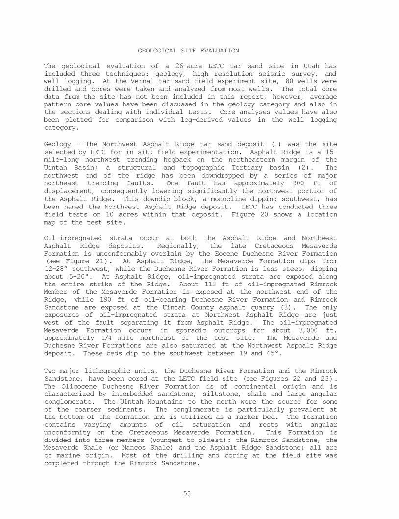
26 "Yellow" Horizon Contour Map 63
27 "Orange" Horizon Contour Map 64
28 Selected LETC Tar Sand Well Locations, Asphalt Ridge 65 Area, Utah
29 Rimrock Sandstone Member Gamma Ray Log Correlations 67
30 Rimrock Sandstone Member Gamma Ray Log Correlations 68
31 Well Pattern Showing Bottom Hole Locations for 74
Experiment TS-1C
32 Temperature History of the Center Production Well 79
33 Temperature Histories, Bottom of Production 80 Wells
34 Temperature Histories at the Mid-Points of the 81 Tar Sand Interval of the Temperature Monitor Wells
35 Temperature Histories, Monitor Well 4 82
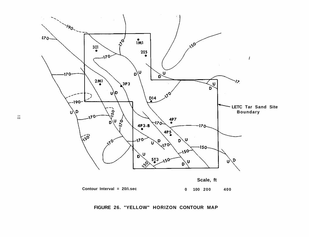
36 Estimated Extent of Heated Tar Sand 84
37 TS-2C Well Pattern Configuration 88
38 300 °F Isotherms for Test TS-2C 94
39 Maximum Temperature vs. Time in Well 203, Test TS-2C 95
40 1000°F Isotherms in a Part of the TS-2.C Test Pattern 102
41 Oil Production Rates, Test TS-2C 104
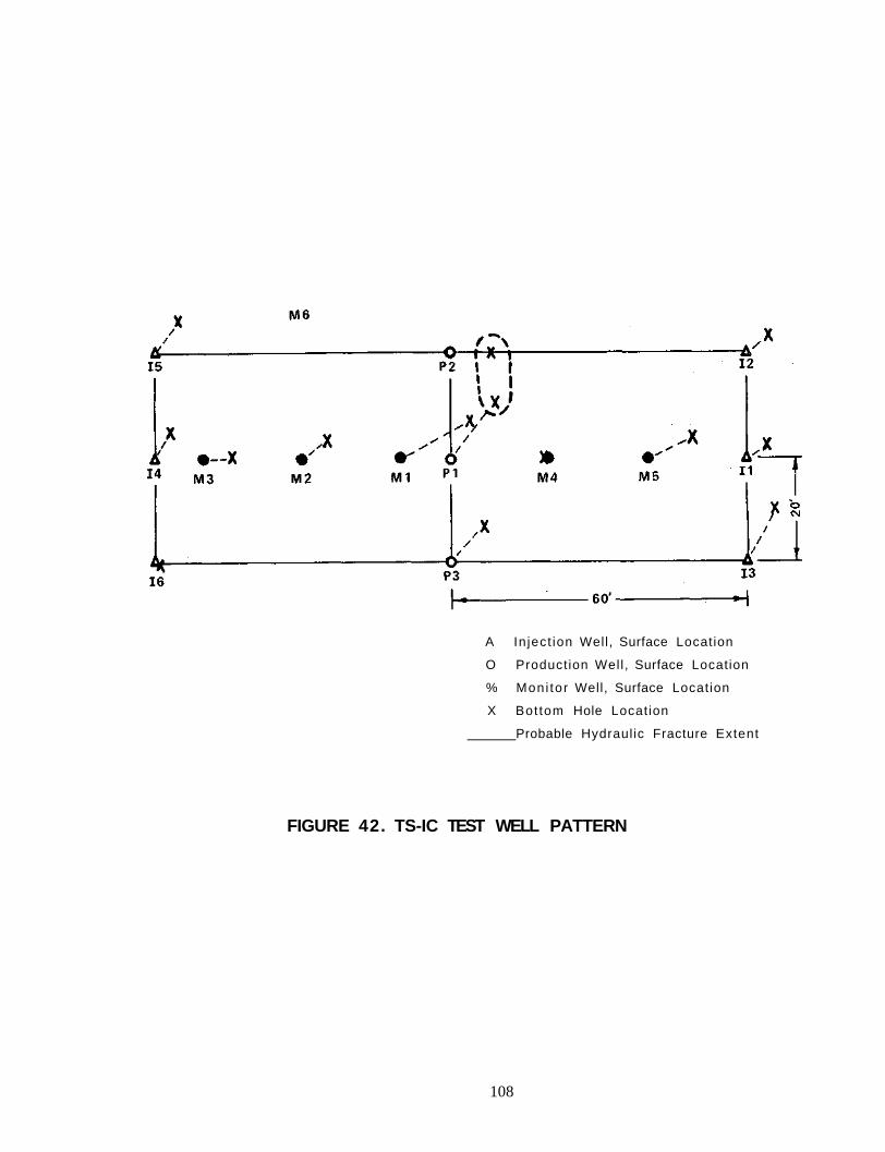
42 TS-1C Test Well Pattern 108
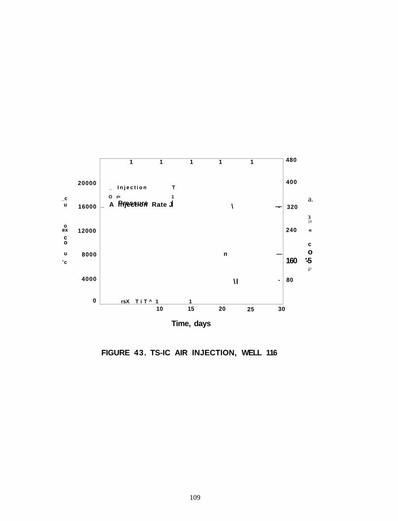
43 TS-1C Air Injection, Well 116 109
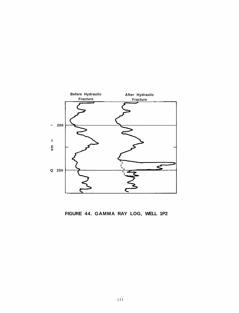
44 Gamma Ray Log, Well 1P2 Ill
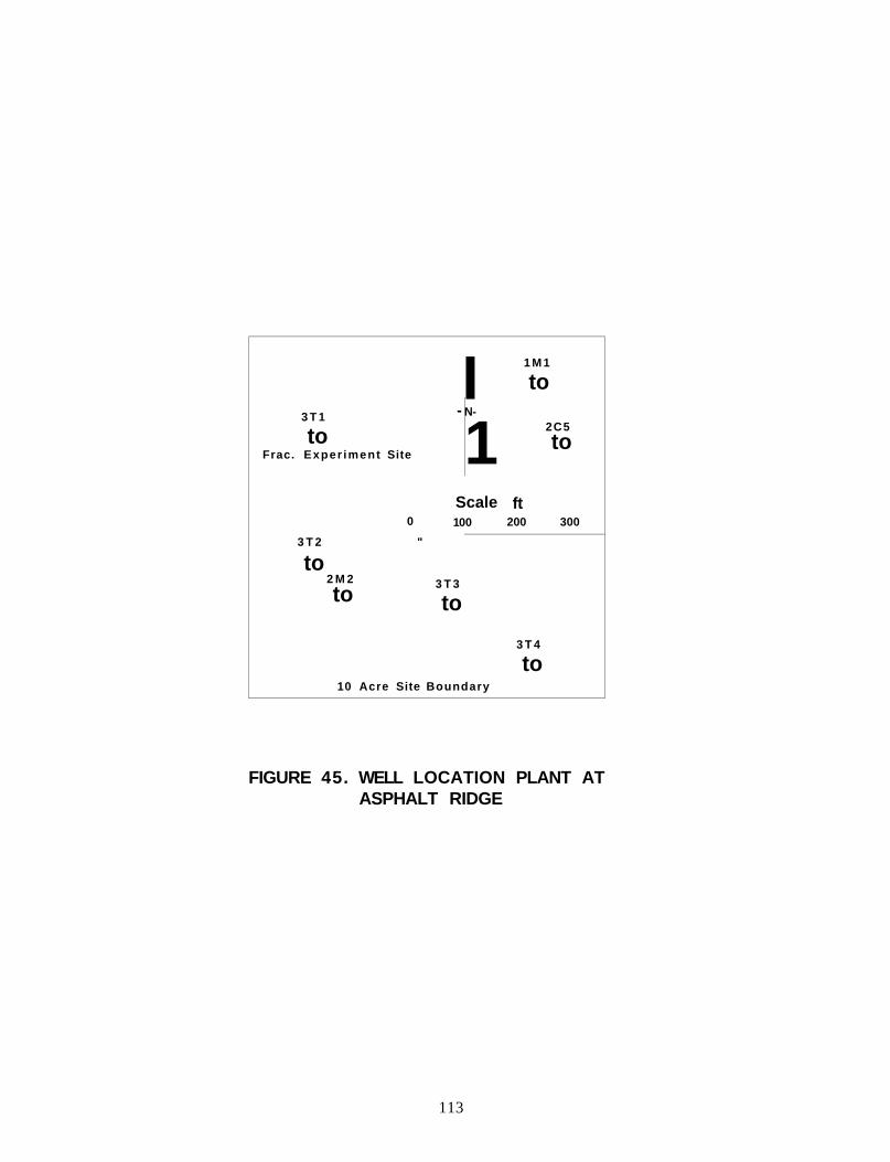
45 Well Location Plant at Asphalt Ridge 113
v
46 Hydraulic Fracture Treatment Log 116
47 Layout of Tiltmeter Holes Around Wei] 3T1 117
48 Filtered Tilt Record 118
49 LETC-SIT Steam Injection Test 123
50 Calculated Bottom Hole Temperature, SIT Test 124
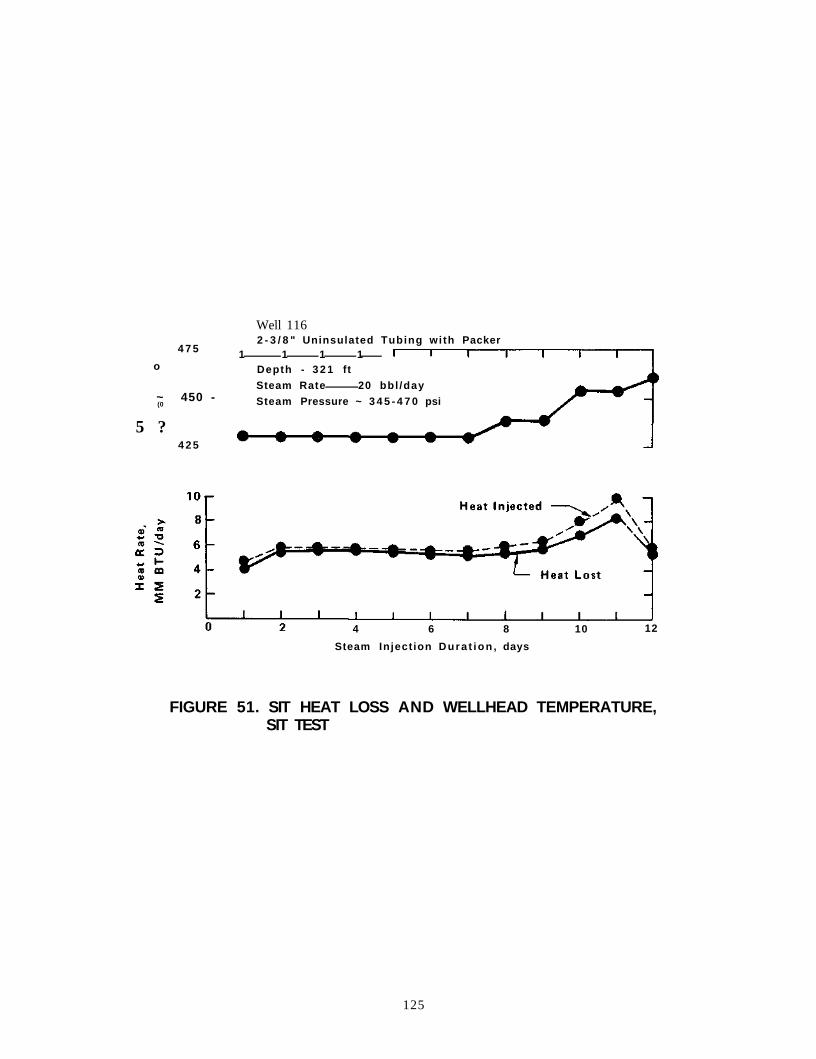
51 SIT Heat Loss and Wellhead Temperature, SIT Test 125
52 TS-1S Test Well Pattern 135
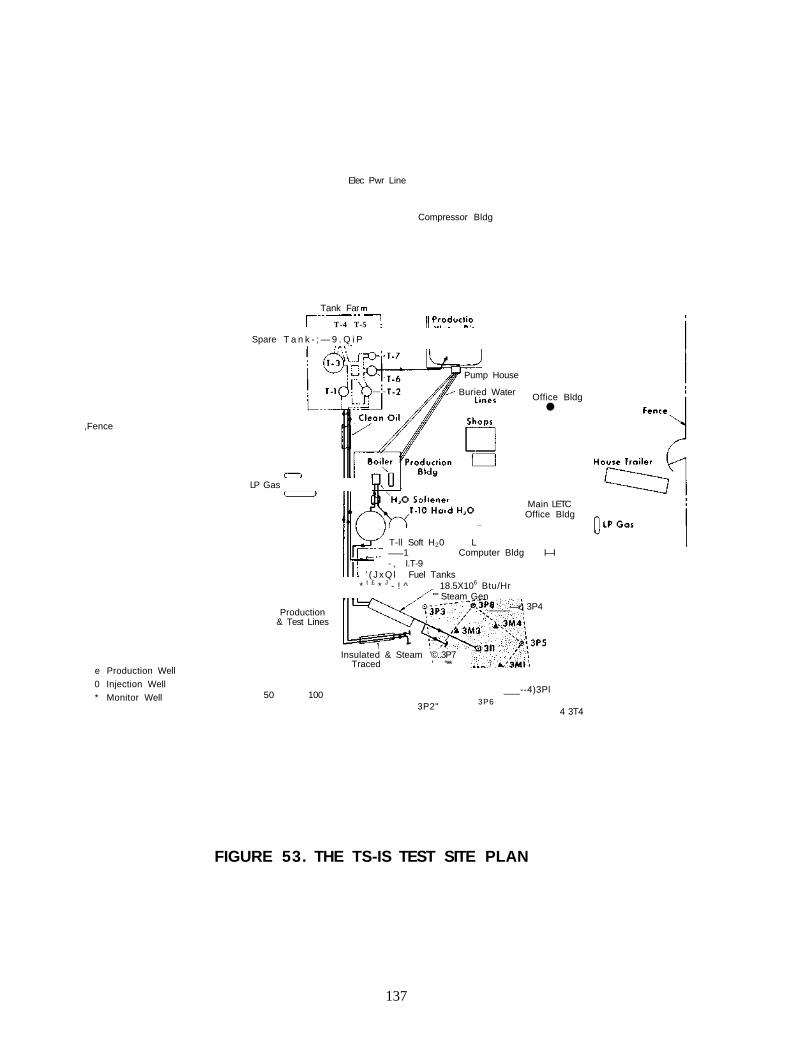
53 The TS-1S Test Site Plan 137
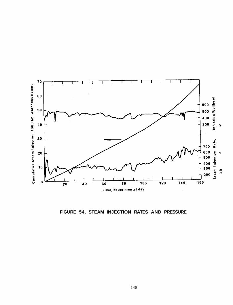
54 Steam Injection Rates and Pressure 140
55 Temperature Profile, Well 3M3 141
56 Hot Water and Steam Zone Locations from Coreholes 143
After the Test
57 Cumulative Water and Oil Production 146
58 Proposed TS-4 Well Pattern 150 59 Pilot Areal Cross-Sectional Grid System 153
60 A Cross-Sectional Grid System for a Field Pattern 154
61 Estimated Effect of Site Sizes on Oil Recovery 163
62 Flame Front Velocity as a Function of Air Flux 183
63 Consumption of Air and Fuel as a Function of Air Flux 184
64 Well Pattern for a Full Scale Line Drive Project 186
65 Schematic Diagram of an In Situ Tar Sand Project 188
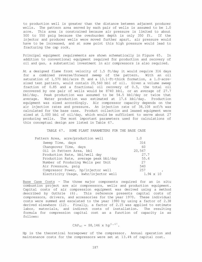
66 Sensitivity of Product Cost to Rate of Return on 191 Investment
67 Sensitivity of Product Cost to Original Site Oil 192 Concentration
68 Sensitivity of Product Cost to Site Pattern Area 193
69 Sensitivity of Product Cost to Percent Oil Recovery 195
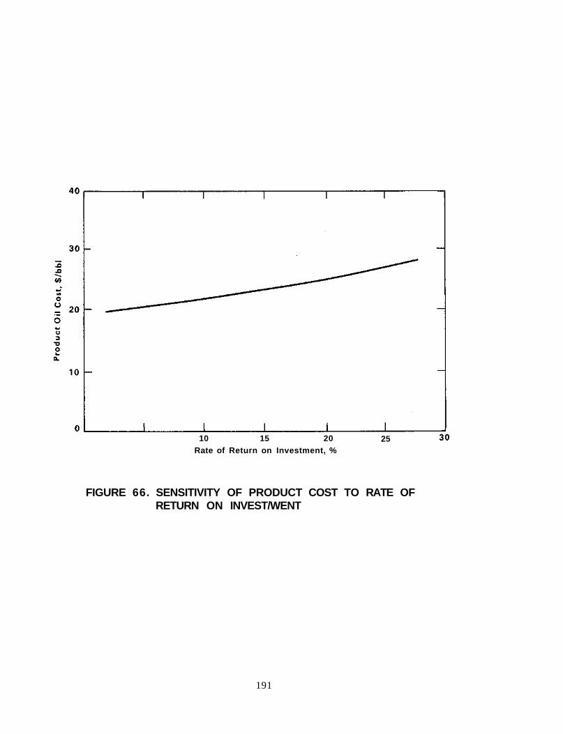
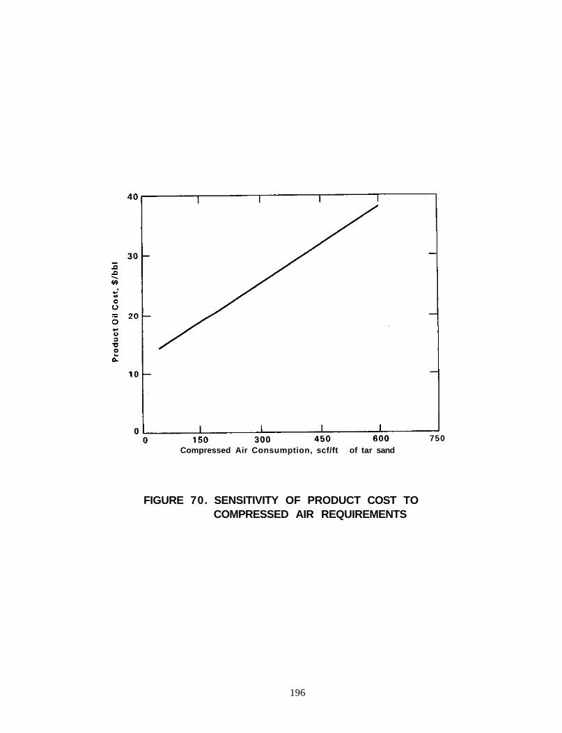
70 Sensitivity of Product Cost to Compressed Air 196 Requirements
vi
LIST OF TABLES
Table Page
1 Organic Content of Four Tar Sand Samples, Wt % 13
2 Properties of Four Tar Sand Bitumens 14
3 Simulated Distillation of Tar Sand Bitumens, Wt % and 16 Cumulative Wt % of Bitumens Distilled
4 Identified Regions of Wells 3T2, 3T3, and 3T4, Northwest 18 Asphalt Ridge
5 Values of Measured Physical Properties from Wells 3T2, 19 3T3, and 3T4, Northwest Asphalt Ridge
6 Values of Parameters Used in Calculations with Zero Order 36 Reaction
7 Values of Parameters Used in Calculations with First Order . . . .38 Reaction
8 Experimental Conditions, Watts Hot Water-Flood Tests 40
9 Simulated Distillation Data From Run 3 42
10 Simulated Distillation Data From Run 8 42
11 Simulated Distillation Data From Run 7 (Nitrogen) 45
12 Oil Saturation in Northwest Asphalt Ridge Tar Sand 45 After Steam-Flood
13 Well Logging and Coring Summary, Northwest Asphalt Ridge 66
14 Drilling and Completion Resume, TS-1C Pattern. 75
15 Average Properties from Core Analyses 76
16 Average Front Velocities 83
17 Average Gas Analyses 83
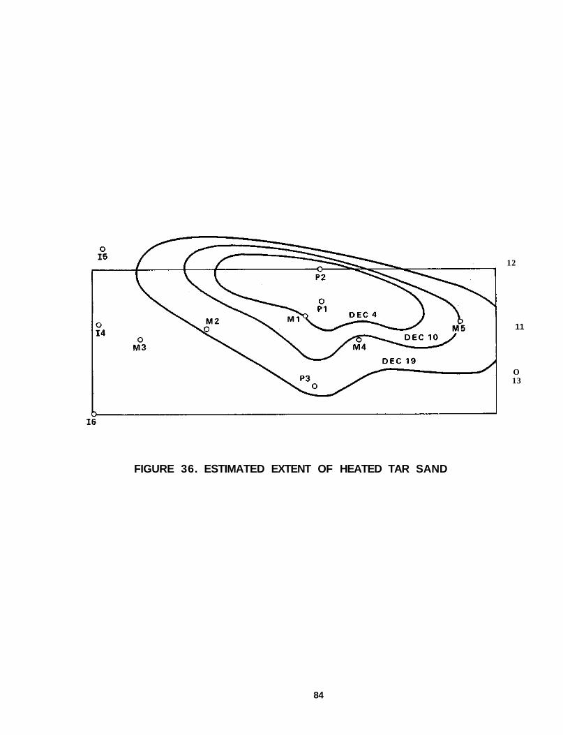
18 Drilling and Casing Resume, TS-2C Pattern 90
19 TS-2C Post-Test Drilling and Coring Resume 91
20 Average Reservoir and Oil Properties 91
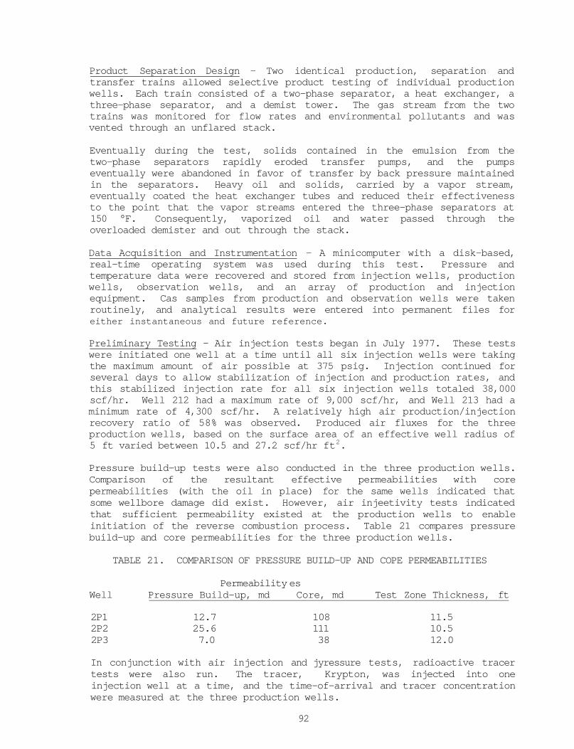
21 Comparison of Pressure Build-up and Core Permeabilities 92
22 Physical Properties of Bitumens and Produced Oils 97
vii
23 Elemental Analyses and Carbon/Hydrogen Ratio of the 98 Bitumen and Produced Oils
24 Results of SAPA Analyses of the Bitumen and Produced Oils . . . 98
25 Results of Distillation of the Bitumen and Produced Oils. . . . 100
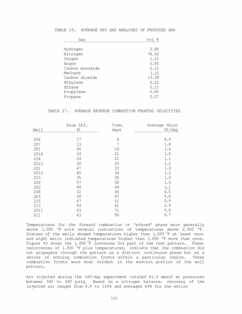
26 Average Dry Gas Analyses of Produced Gas 101
27 Average Reverse Combustion Frontal Velocities 101
28 Average Reservoir Properties, TS-1C Test Site 107
29 Hydraulic Fracture Treatment Data, First Test on 110 TS-1C Site
30 Fracture Treatment Log 110
31 Fracture Treatment Design Summary 115
32 LETC Steam Injection Test (SIT) 126
33 Analyses of the Oil Produced During the SIT Test 127
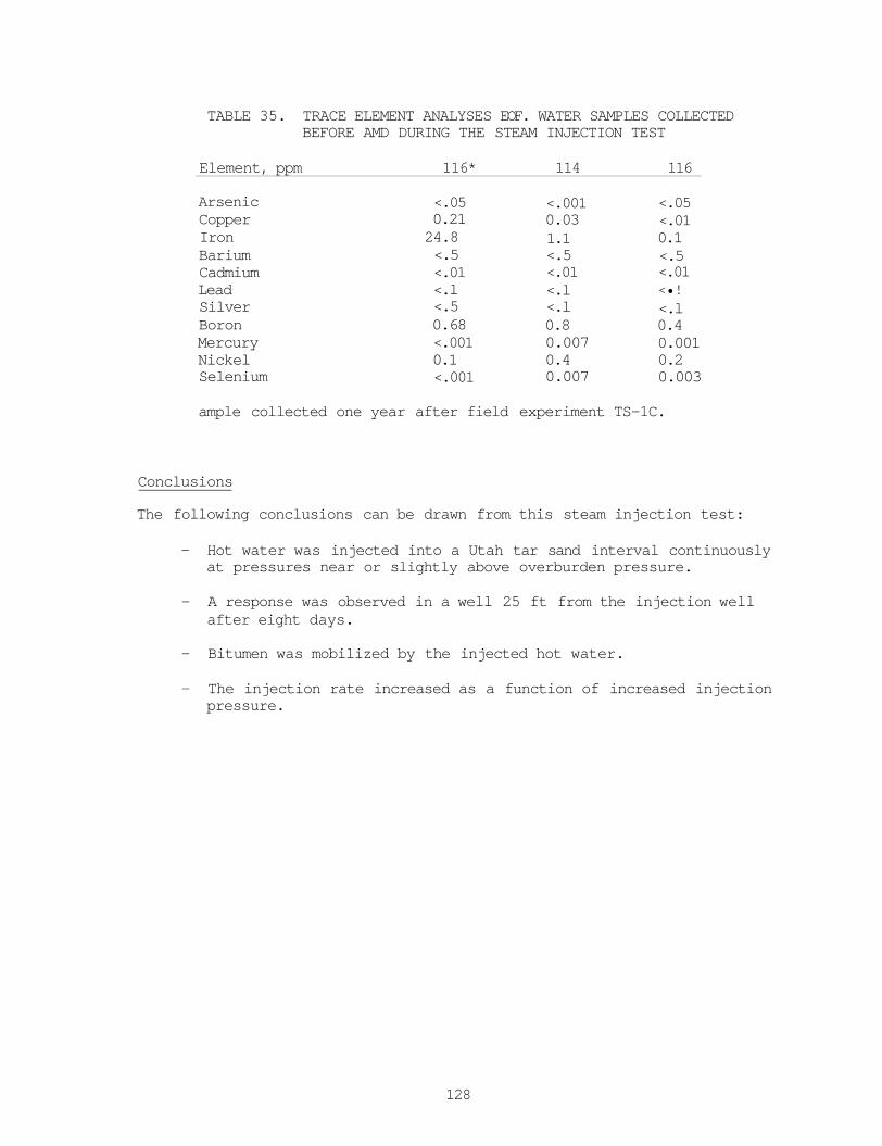
34 Water Quality Analyses for Samples Collected Before . . . . . . . 127 and During the Steam Injection Test
35 Trace Element Analyses for Water Samples Collected. . . . . . . 128 Before and During the Steam Injection Test
36 Well Elevations 131
37 Test Core Holes 132
38 Average Reservoir and Oil Properties 134
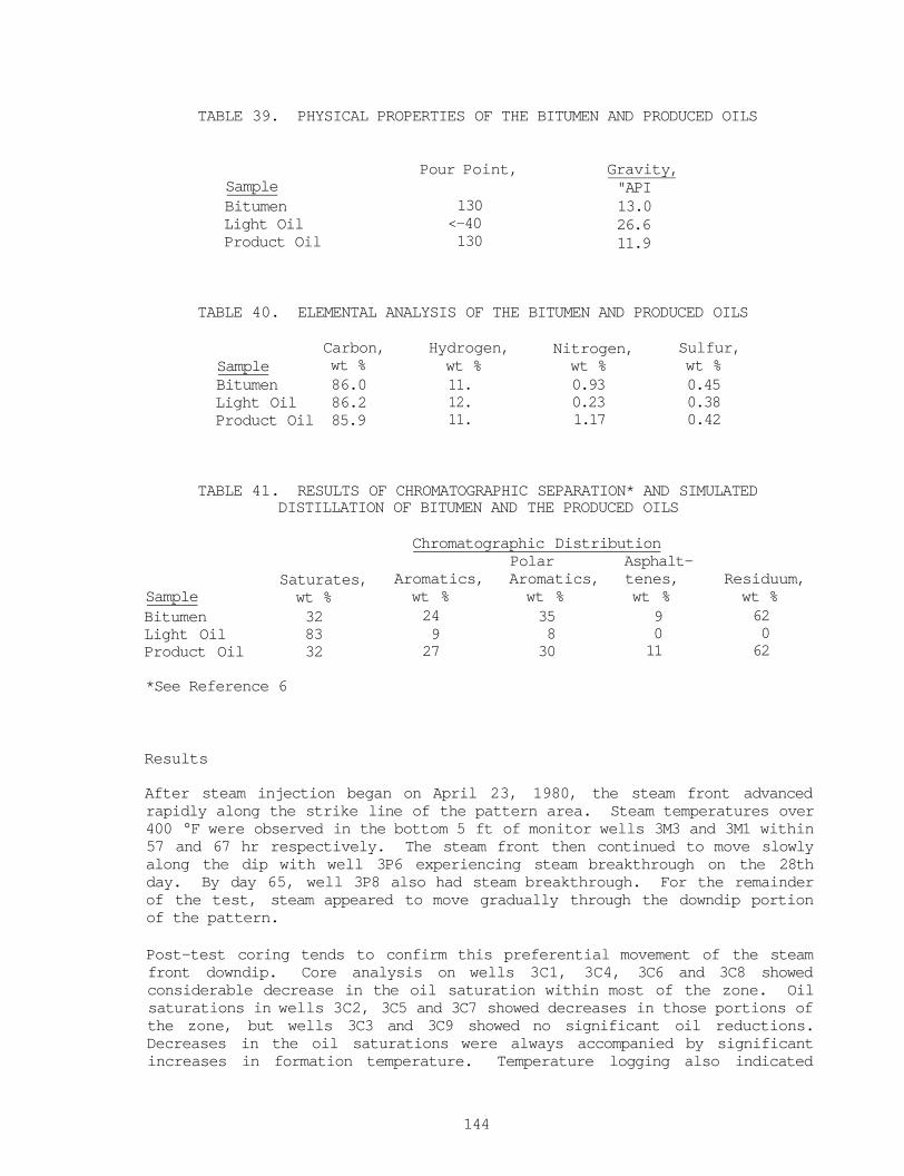
39 Physical Properties of the Bitumen and Produced Oils 144
40 Elemental Analysis of the Bitumen and Produced Oils 144
41 Results of Chromatographic Separation and Simulated 144 Distillation of Bitumen and thpsProduced Oils
42 Experimental Results 145
43 Analyses of Bitumen and Oil Pyrolysls, Northwest Asphalt . . . .151 Ridge Tar Sand
44 Average Reservoir Properties, Upper Rimrock, Northwest Asphalt. 152 Ridge, Uintah County, Utah
45 Optimization of Two-Acre Reverse Combustion Results 156
46 Optimization of Pattern Sizes For Reverse Combustion 156
viii
47 Viscosity Effects in Pilot Reverse Combustion: Performance . . 157 Comparison of Runs 6 & 10
48 Viscosity Effects in Field Reverse Combustion: Performance . . 157 Comparison of Runs 8 & 9
49 Optimization of Two-Acre Steam-Flood Results 158
50 Optimization of Pattern Sizes for Steam-Flooding 159
51 Viscosity Effects in Field Steam-Flooding: Performance 160 Comparison of Runs 8 & 9
52 Effect of Pre-Heat Combustion in Pilot Results: 161 Performance Comparison of Runs 3 & 11
53 Effect of Pre-Heat Combustion in Field Results: 162 Performance Comparison of Runs 10 & 12
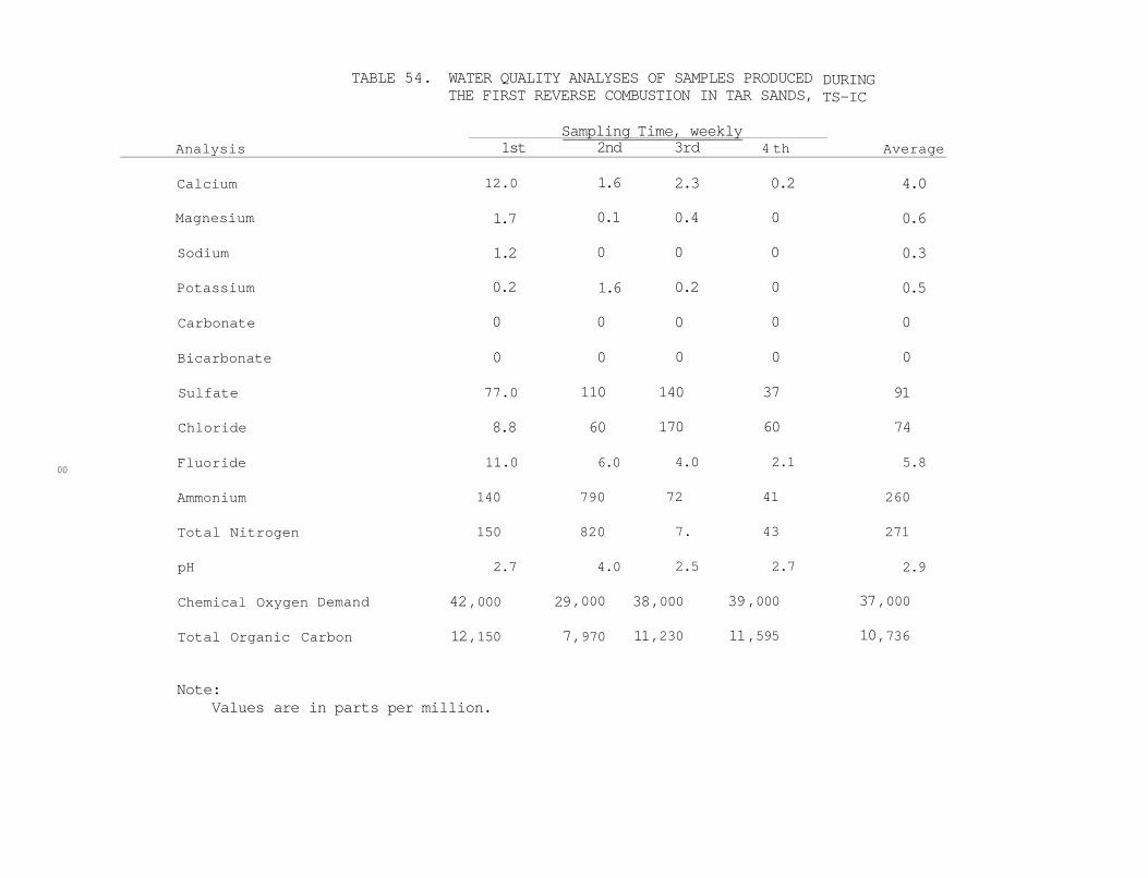
54 Water Quality Analyses of Samples Produced During 168 the First Reverse Combustion in Tar Sands, TS-1C
55 Trace Element Analyses of Water Samples Produced During . . . . 169 the First Reverse Combustion in Tar Sands, TS-1C
56 Elemental Analyses by Spark Source Mass Spectroscopy of . . . . 170 Water Samples Produced During the First Reverse Combustion Test, TS-1C
57 Major Components Identified in the Base Extract of Water . . . 171 Collected from the First Tar Sands Experiment, TS-1C
58 Major Components Identified in the Acid Extract from 171 Water Collected During the First Tar Sands Experiment, TS-1C
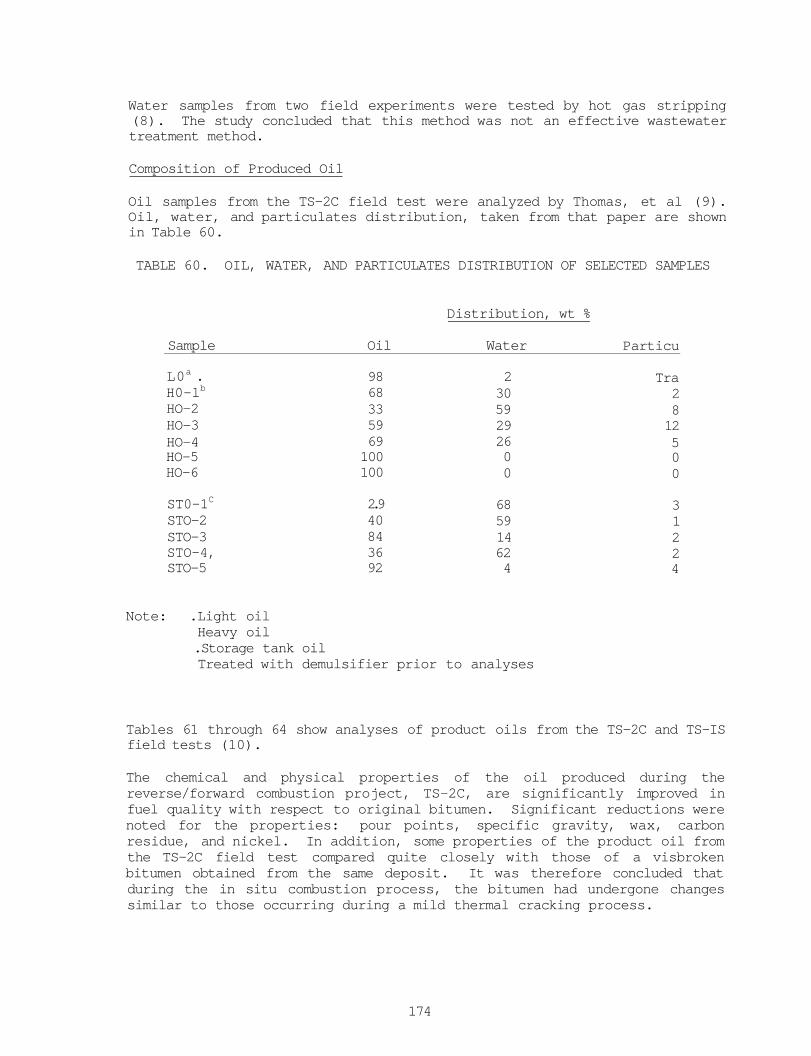
59 Analyses of Six Water Samples from the TS-2C Test 172
60 Oil, Water, and Particulates Distribution of Selected 174 Samples
61 Physical Properties of the Bitumen and Oils Produced 175 During the TS-2C and TS-1S Tests
62 Components Analyses of the Bitumen and Oils Produced 176 During the TS-2C and TS-1S Tests
63 Elemental Composition and Carbon/Hydrocarbon Ratios 177 of the Bitumen and Oils Produced During the TS-2C and TS-1S Tests
64 Simulated Distillation Analyses of Bitumen and Oils 178 Produced During the TS-2C and TS-1S Tests
ix
65 Average Reservoir and Oil Properties in the Northwest 181
Asphalt Ridge Deposit
66 Process Parameters for the Base Case 185
67 Some Plant Parameters for the Base Case 187
68 Base Case Cost Data 189
x
EXECUTIVE SUMMARY
This report describes work done by the United States Department of Energy's Laramie Energy Technology Center (LETC) from 1971 through 1982 to develop technology for future recovery of oil from U.S. tar sands. Work was concentrated on major U.S. tar sand deposits that are found in Utah. Major objectives of the program were as follows:
- Determine the feasibility of in situ recovery methods applied to tar sand deposits.
- Establish a system for classifying tar sand deposits relative to those characteristics that would affect the design and operation of various in situ recovery processes.
Most of the world's supply of tar sand is found in the Western Hemisphere, and deposits in Venezuela and Columbia are estimated to exceed 1 trillion barrels. Canadian deposits are estimated at 967 billion barrels in the Province of Alberta. The U.S. tar sand deposits are estimated to be over 53 billion barrels, with over 20 billion barrels found in Utah. Estimates have been made that only 10% of the U.S. tar sand can be recovered by surface mining, and 90% must be recovered by in situ methods.
Early work at LETC included physical and chemical characterizations of Utah tar sand. Tar sand is bitumen-bearing rock with an in-place viscosity exceeding 10,000 centipoises at reservoir temperature. Athabasca (Canadian) tar sand is a water wetted sand and therefore is amenable to water-based extraction processes, while many U.S. tar sand deposits are oil wetted sands that require different approaches to oil recovery. The U.S. tar sand typically contains 5 to 10 wt % bitumen. Uintah Basin, Utah bitumen is low in sulfur content (less than 1%) compared to Athabasca and other U.S. bitumens.
Laboratory work at LETC was conducted to gain insight into methods for reduction of viscosity necessary to better recover bitumen from Utah tar sand. These experiments showed that reverse combustion could be used to open and heat a flow path from a well bore into a tar sand deposit. Air flux rates necessary to sustain combustion were determined and oil yields were shown to be encouraging. A mathematical model of the reverse combustion process was developed and used to design other field experiments.
Later laboratory work was also conducted with steam injection into Utah tar sand samples. Results showed that the mechanisms associated with a hot water flood are part of the steam drive recovery mechanism. Steam drive recovery of oil was also shown to have the added advantage of a solvent extraction mechanism working to increase the recovery of oil over that which would be expected from a hot, water flood. This work, combined with a steam drive simulator, was used to design and operate one field experiment described later in this report.
1
The site selected for field experiments was located 4 miles west of Vernal, Utah, on property owned by Standard Oil of Ohio (S0H10). This site was located on the Northwest Asphalt Ridge Deposit where tests were conducted in the Rimrock Sandstone Member of the Mesaverde Formation at depths of 300 to 500 feet. The Rimrock Sandstone is a highly saturated, semi-consolidated to consolidated, fine-grained sandstone with claystone, siltstone, and shale intervals. At the test site the Rimrock Sandstone contains continuous tar sand sections varying in thickness from less than 1 foot to more than 40 feet. The Rimrock Sandstone is heavily faulted in this area and dips steeply to the southwest at angles anywhere from 10 to 45°.
Core analyses and logging techniques were used to evaluate reservoir properties of proposed test locations in the deposit. Core analyses were initially used to determine porosity, oil and water saturation, and permeability for the design of the experiments. A gamma, sidewall neutron, density, SP, induction and caliper log suite were utilized in determining porosity and water saturations. A sonic log was used to determine elastic rock properties for design of a hydraulic fracture. Carbon/oxygen logs were used to measure oil saturation before and after recovery tests. The best porosity values were determined from the density log. Formation water resistivity was estimated from the Archie equation using core porosity, water saturation and the induction log formation resistivity. Water saturation was acceptable, but it did not match core data as well as desired. Oil saturation values from the carbon/oxygen log may be conservative because of the lack of a reference unsaturated clean sandstone.
Associated environmental research characterized the emissions generated from the field experiments and aided in developing a technology for controlling those emissions. Emphasis in environmental research was on water cleanup technologies that would make process water available for use as steam. Generally this work showed that waters from in situ tar sand recovery experiments can be cleaned up using existing technology, and biological oxidation of process water was shown to be an effective treatment option. Activated sludge treatment was found to be an effective method for reducing the organic content of process water.
The TS-1C field experiment (the first one) was conducted in the fall and winter of 1975. The objectives for this test were to demonstrate the feasibility of reverse combustion as a method of recovering oil from a tar sand deposit and to gain experience with heavy oil recovery equipment. Combustion was initiated in the middle wells of the unenclosed line drive pattern at a depth of 300 ft. It was necessary to inject air at pressures higher than lithostatic pressure to obtain the desired injection rates. Produced oil was not cracked as much as had been hoped or anticipated and plugging of surface recovery equipment became a major problem. Combustion was sustained for 63 days before the experiment was terminated after it was concluded that little additional information would be gained from continued operation. A total of 60 barrels of heavy oil were recovered and approximately 84 percent of the injected air was lost to the formation. It became apparent that better provisions for handling heavy oil would be needed in any future experiments.
2
For the second field experiment, TS-2.C, the test pattern was laid out along the strike line of the formation to take advantage of directional permeability to increase injection rates and minimize air losses to the formation. Recovery equipment was provided with heating capability to handle heavy oil. The experiment was designed to use a reverse combustion phase to prepare the tar sand zone, followed by forward combustion, which was supposed to drive the bitumen to producing wells.
This second experiment was ignited in August, 1977, and continued for 183 days. Problems were encountered with production equipment failure, wellbore plugging, and formation heterogeneity. Propagation of the reverse combustion front did not occur as a distinct continuous phase; rather it occurred as several echoings of two combustion phases, both reverse and forward within the same area. Recovery of injected air averaged 49% for the experiment. The experiment produced 580 barrels of oil, or 25% of the original oil in place. Volumetric sweep efficiency was calculated to be 86% for reverse combustion and 33% for forward combustion. This second field effort was considered to be a successful experiment and provided encouragement for further improvement in the reverse-forward combustion technique.
A hydraulic fracture was tested in 1978 as a possible means of increasing permeability within a highly saturated tar sand zone. The fracture was designed from data collected from oriented core and from log-derived elastic properties. Real time evaluation of the fracture growth was monitored by surface tiltmeters. Post fracture evaluation was conducted from wells drilled to intersect the fracture and included air flow tests, TV logging, sonic logging, and casing cement bond logging. It was concluded that the fracture was dominated by a nearby fault and a zone of high permeability within the conglomerate that was on top of the tar sand zone. The fracture did not achieve the size or orientation desired due to the heterogeneity of the site.
A two-well steam injection test was conducted in 1979, and this test showed that steam injection rates sufficient for a steam drive could be achieved. It also showed that bitumen could be mobilized with hot water.
On the basis of this two-well steam test, a steam-flood field experiment was planned with the objectives of 1) determining the technical and economic feasibility of using a steam-flood as an in situ recovery technique in a Utah tar sand deposit, ?.) evaluating an injection well completion using a high temperature packer, 3) evaluating several production well completion schemes, and 4) determining recycle and fuel use possibilities for produced water and oil. The steam-flood experiment, TS-1S, was designed using data from previous experiments, laboratory studies, computer modeling, and the two-well steam injection test. The well pattern selected included two concentric, inverted five spots, one on one-fourth acre, and the other on one-tenth acre sites.
The steam-flood test (the third field test in this series) began in April, 1980, and continued until late September, 1980. A 45—foot thick interval of tar sand located about 500 feet below the surface in the Rimrock Sandstone was the target area. The steam front was observed to move preferentially down dip, and some steam was lost to the overburden through
3
faulty casing cement. A major portion of the injected steam was lost to the underburden. Both heavy oil and light oil were recovered during the test.
The overall steam efficiency for the pattern was about 16 percent. A small portion of the 1,150 barrels of oil produced was light oil, probably produced by steam distillation. Major oil production, similar in properties to the original bitumen, resulted from hot water displacement.
A fourth field experiment, TS-4, was designed in late 1981 and early 1982. This experiment, planned for the SOHIO property, was planned to use the best features of in situ combustion to preheat the reservoir and then steam-flooding to produce oil. Data from laboratory and field experiments were used in computer model runs to evaluate a series of alternative design conditions. Generally, the model runs showed that if a 10-foot interval of high permeability were preheated by reverse combustion, and a steam drive was then applied to the 65-foot tar sand zone, about 40 percent of the original oil-in-place could be recovered. The model runs also showed the importance of high injection rates to increase the rate of oil recovery and to reduce heat losses. This field experiment was planned but never conducted.
This report covers in detail all field experiments conducted by LETC in Utah, as well as the geology and characterization of some Utah Tar Sand deposits. Environmental research done in parallel with the field experiments, as well as an economic evaluation of in situ oil recovery from tar sand, are also presented.
4
INTRODUCTION
Shown dramatically by the 1970's crisis involving petroleum and natural gas, shortages and rising prices foreshadow an end to unlimited consumption of natural resources at traditionally low prices. Alleviating these growing shortages of fossil fuels will require increased production from traditional sources and development of new sources. These new sources include oil from tar sand and oil shale, and gas from gasification of coal.
The U.S. tar sand resource and related recovery technology has never been a target of a major research effort by the private sector, perhaps because most of the known resource is on federal land. Due to this low level of activity by the petroleum industry to develop the domestic tar sand resource, the United States Department of Energy's Laramie Energy Research Center (LERC) in 1971 began working with a tar sand resource in Utah. The initial work consisted of the definition, characterization and analyses of deposits and determination of the most promising recovery methods to test. Specifically the two major program objectives were as follows:
- Determine the feasibility of in situ oil recovery methods applied to tar sand.
Establish a system for classifying tar sand deposits relative to those characteristics that would affect the design and operation of various in situ recovery processes.
The term "tar sand", which is used in this study, is a commonly used descriptive phrase applied to a wide variety of hydrocarbon-bearing rocks. However, the term "tar sand" is a classic misnomer because tar is a refined hydrocarbon substance and sand is a fine unconsolidated particulate mineral material. Therefore, a more appropriate term could be "bitumen-bearing rock", and one suitable definition of this type of material could be: "A consolidated to unconsolidated rock that contains in its pore space a viscous, semi-solid to solid bitumen that cannot be produced in its natural state by known petroleum production processes". Bitumen refers to an organic material that is soluble in an organic solvent and has an in-place viscosity at reservoir temperature greater than 10,000 centipoises. This definition would not include non-asphaltic rocks such as gilsonite, oil shale or coal.
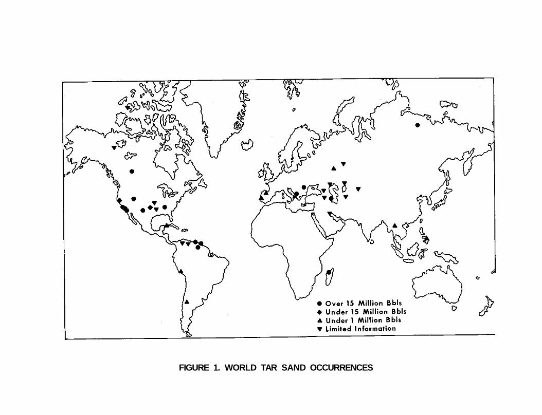
Tar sand is found throughout the world (see Figure 1) with most of the resource located in the Western Hemisphere (1). Tar Sand deposits in Venezuela and Columbia contain an estimated 1.0 to 1.7 trillion barrels of oil (2). Deposits in Alberta, Canada, are estimated to contain (see Figure 2) 967 billion barrels of oil (3). The United States tar sand resource is estimated to contain about 53 billion barrels of oil (4) in over 500 deposits in 22 states, and deposits in the State of Utah (see Figure 3) alone contain in excess of 20 billion barrels of oil or about 40% of the United States total.
5
FIGURE 1. WORLD TAR SAND OCCURRENCES
Names of Major World Tar Sand Deposits Shown in Figure 1
North America
Melville Fort Good Alberta:
Island Hope Athabasca Peace River Wabasca Cold Lake
Point Arena Santa Cruz Edna Sisquoc Utah: Sunnyside
Asphalt Ridge P.R. Spring Tar Sand Triangle Hill Creek Circle Cliffs
Santa Rosa Sulfur Pleasonton Pike Kentucky:
Pinar del
Asphalt Davis-Dismal Creek Kyrock Rio
Europe
Monte Real Santander-Alava Prov. Scienizza Derna
Asia
Notanebi Tiflis Kobystan W. Uzbekistan Fergana Kazakhistan Zolnyy Simbirsk Subovka Olenek Burgan Melang Leyte
Africa
South America
Bemolanga
Incarte Bolivar Coastal Fields Guanco Oficina-Temblador La Brea Chumpi San Raphael
7
ALBERTA
ATHABASCA <9
O a
PEACE RIVER
WABASCA
Miles
•Calgary
FIGURE 2. MAJOR CANADIAN TAR SAND DEPOSITS
<£
UTAH
Asphalt Ridge
Sunnyside
fef'nRsgM'
Well Mapped and Continuous Deposits
Areas Containing Smaller and Dispersed Deposits
Tar Sand Triangle
Circle Cliffs
**&
FIGURE 3. MAJOR UTAH TAR SAND DEPOSITS
The tar sand deposits of Utah are located in two general areas; in the Uintah Basin and in the central-southeast. The location of individual deposits and extent of reserves have been identified by H.R. Ritzma, who was formerly with the Utah Geological and Mineralogical Survey (5). Of the 20 billion barrels of bitumen (oil) contained in Utah tar sands, 10.8 billion barrels are contained in the Uintah Basin deposits, principally Asphalt Ridge, Hill Creek, Sunnyside, and P.R. Spring. The major deposits of the central-southeast portion are Circle Cliffs and the Tar Sand Triangle.
The bitumen (oil) found in Uintah Basin tar sands is believed to have originated in the lacustrine Green River Formation and are of non-marine origin, i.e. the organic precursor material is that of fresh water aquatic life. The principal formations containing bitumen in the Uintah Basin are of the Eocene age, with the tar sands of the Asphalt Ridge area present in formations of both the Eocene and Upper Cretaceous age. In the central-southeast area, the bitumen is of a marine origin and is similar to properties of Athabasca, Canada, tar sand bitumen, which is also believed to be of a marine origin. The Circle Cliffs bitumen is found in the Moenkopi Formation (Triassic age) and Tar Sand Triangle bitumen is found predominantly in the White Rim Member of the Cutler Formation (Permian age) .
Of the total U.S. tar sand resource, an estimated 10% could be recovered by surface mining and above-ground extraction techniques. To recover the remaining 90%, in situ process techniques will have to be used. These vary from the conventional thermal recovery methods used for heavy oil production to exotic in situ methods, such as microbial degradation microwave heating. Economics may dictate that a combination of mining and in situ processes will have to be used in some deposits.
10
REFERENCES
Phizackerley, P. H. and L. 0. Scott. "Major Tar Sand Deposits of the World." Proceedings: 7th World Petroleum Congress, Mexico, V. 3, 1967, pp. 551-571.
Arscott, R. L. and A. David. "An Evaluation of In-Situ Recovery of Tar Sands." In Situ, V. 1, No. 3, 1977, pp. 249-266.
Alberta Department of Energy and Natural Resources. "Alberta Oil Sands Facts and Figures." Department of Energy and Natural Resources, Alberta, Canada, ENR Report No. 110, 1979, 67 pp.
Marchant, L. C, G. J. Stosur and C. Q. Cupps. "Recent Activity in U.S. Tar Sand." Proceedings: 15th Intersociety Energy Conversion Engineering Conference, Seattle, Washington, 1980, 10 pp.
Ritzma, H. R. "Oil-Impregnated Rock Deposits of Utah." Utah Geological and Mineral Survey, UGMS Map 47, Jan. 1979.
11
CHARACTERIZATION OF UTAH TAR SAND
The physical and chemical properties of tar sand bitumens ultimately determine their value because these properties influence the recovery, processing, conversion, and utilization of fossil energy resources. This section contains information on bitumen characterization and tar sand core properties.
Source and Preparation of Samples - Tar Sand samples were obtained from Northwest Asphalt Ridge, Tar Sand Triangle, P.R. Spring, and Athabasca, in Alberta, Canada. The exact source of each sample is listed elsewhere (1,2).
New extraction procedures used to separate bitumen from sand were developed to minimize changes in bitumen properties during the extraction process and to produce reproducible bitumen samples. To assure that a high percentage of the organic material present in the original tar sand sample had been accounted for, procedures were adopted to recover most of the light ends as well as species that strongly adsorbed on the sand.
The sample was extracted with benzene in a Soxhlet extractor. The benzene extract was filtered through a 4.0-5.5 u fritted glass disk funnel, and the benzene was removed by rotary evaporation. Light ends, which may have been distilled during solvent removal, were recovered by redistilling the solvent concentrate on a spinning band column with the efficiency of 100 theoretical plates. Material insoluble in benzene and/or strongly adsorbed on the sand was recovered by further extraction with pyridine.
Table 1 lists the percentage of benzene and pyridine extractables and the percentage of light ends recovered. Neither the light ends nor the pyridine extracts were added to the benzene extracts for characterization. However, the characterization of any given sample was performed on at least 95% of the total extractable bitumen.
Properties and Elemental Analysis - Table 2 lists the physical properties and the elemental analyses for the four tar sand bitumens studied. Results of elemental analyses are similar to values obtained by other investigators (3-8). The Athabasca and Tar Sand Triangle bitumens are high in sulfur and low in nitrogen compared to the Uintah Basin materials from Northwest Asphalt Ridge and P.R. Spring. The nitrogen contents for these particular samples are in the range observed for other bitumens from their respective deposits. The sulfur content of the Tar Sand Triangle sample (4.38%) is typical of bitumens of Permian geologic age.
Vanadium and nickel contents are important to catalytic refining processes. Results of analyses show that vanadium content is low for the low-sulfur Uintah Basin samples. Except for the correlation of vanadium content with sulfur content often observed in petroleum samples, no other obvious trends exist.
Ash yield and specific gravities are generally low compared to some literature values for tar sand bitumens (7,8,10). This could be explained by the lower content of minerals present in the bitumens of this study because of more efficient filtration. Although the viscosity values reported may not accurately represent the viscosity of in-place bitumen,
12
TABLE 1. ORGANIC CONTENT OF FOUR TAR SAND SAMPLES, WT %
Benzene extracted Pyridine Total Ratio, bitumen/ Bitumen Light Ends Extracted Organics total orgaincs
Penetration, 1/10 mm 50 g 77°F Dynamic viscosity, poise Carbon residue, Ramsbottom, wt % Asphaltenes, wt %
Heating value, btu/lb Measured Calculated
Athabasca
82.57 10.28 0.47 4.86 1.78 0.02 0.674
180 112
0.989 11.6
600 6,380
16.11 16.4
17,700 17,800
Tar Sand Triangle
12
17 17
84.04 10.14 0.46 4.38 1.13 0.12 0.696
108 53
0.992 11.1
346 ,990 21.6 26.0
,900 ,900
P R. Spring
325
18 18
84.44 11.05 1.00
0.75 2.20 0.17 0.641 25 98
0.998 10.3
130 ,000 12.5 16.0
,100 ,200
N.W. Asphalt Ridge
85.28 11.72 1.02
0.59 1.14 0.04 0.611 25 120
0.970 14.4
277 29,500
3.5 6.3
18,800 18,800
Average molecular wt, VPO in benzene 568 578 820 668
because of the unknown effects of incomplete removal of the extraction solvent, the loss of light ends, and the exclusion of polar, pyridine extracts, the uniformity by which these samples were extracted and prepared allows for meaningful comparisons between samples.
Carbon residues (Ramsbottom) ranged from a high of 21.6 wt % for the Tar Sand Triangle samples to an extreme low of 3.5 wt % for the sample from Northwest Asphalt Ridge. The carbon residue roughly correlates with the amount of pentane asphaltenes present in the bitumens.
Average molecular weights ranged from 568 to 820. The molecular weight determined for the Athabasca bitumen of 568 is slightly lower than the 600 to 700 reported by Jones and Moote (12). The molecular weights for the Uintah Basin bitumens are higher than those for Athabasca and Tar Sand Triangle samples. This correlates with the higher viscosities and lower volatiles observed for Uintah Basin samples. Because molecular weights, as determined by vapor pressure osmometry, are subject to intermolecular associations, it is almost certain that the molecular weights reported here are in error and higher than the actual values.
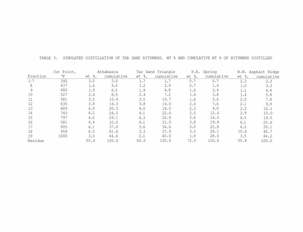
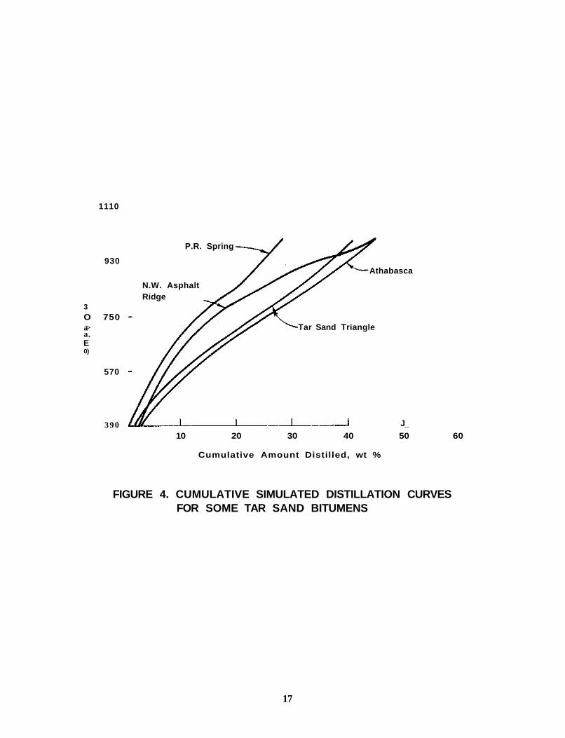
Table 3 lists the simulated distillation data for the four bitumens. These data are compared to data obtained by the Hempel distillation procedure (13), but simulated distillation allows extension to 1000°F without thermal decomposition. The utilization of the flushing technique (14) in the simulated distillation of these high-residue samples has resulted in a difference between those values previously published for the P.R. Spring bitumen (1) and those listed here. It is believed that the present values for the P.R. Spring bitumen are more accurate. The Athabasca and Tar Sand Triangle samples have nearly identical distillation curves throughout the distillable range (see Figure 4). The distillation curves for Northwest Asphalt Ridge and P.R. Spring bitumens are similar up to a temperature of 842°F. The divergence above this temperature is probably due to the presence of a well-defined spike in the Asphalt Ridge sample having a nominal boiling point of 923°F. This peak, present in fraction 18, accounted for 10.6 wt % of the bitumen. The large amount represented by this peak may also be the cause of the lack of correlation between molecular weight and volatility of this sample. This peak has recently been identified as perhydro-g-carotene (15).
Conclusions that now can be drawn from the property and distillation data are as follows: 1) that the four study samples differ significantly in heteroatom content, carbon-hydrogen ratios, viscosity, carbon residue, and asphaltene content; 2) that the bitumens are generally similar in average molecular weight, gravity, and heating value; 3) that a rough correlation exists between average molecular weight, distillation residue content, and viscosity; and 4) that the four individual samples are representative of their respective deposits, based on the similarity of the properties reported here and those reported in the literature (4,7,10,16).
Core Properties A standard core analysis was performed on cores from four wells in the Northwest Asphalt Ridge area. The density, oil-water-sand content, permeability of saturated and extracted cores and porosity of the saturated and extracted cores were found using standard core analysis techniques. Lindberg (18) has summarized the results of these tests. An
15
TABLE 3. SIMULATED DISTILLATION OF TAR SAND BITUMENS, WT % AND CUMULATIVE WT % OF BITUMENS DISTILLED
FIGURE 4. CUMULATIVE SIMULATED DISTILLATION CURVES FOR SOME TAR SAND BITUMENS
17
examination of the oil content for three samples identified distinct zones of high oil content and layered beds of shale-like materials. These natural divisions allowed for identification of four zones for each well, and these zones are listed in Table A as a function of depth. Table 5 contains the results of the core analyses relative to these 12 regions.
TABLE 4. IDENTIFIED REGIONS OF WELLS 3T2, 3T3, AND 3T4, NORTHWEST ASPHALT RIDGE
Region Well No Depth, ft
1 3T4 418 to 443
2 3T4 476 to 495
3 3T4 500 to 541
4 3T4 543 to TD
5 3T3 410 to 452
6 3T3 465 to 483
7 3T3 488 to 535
8 3T3 539 to TD
9 3T2 445 to 475
10 3T2 486 to 512
11 3T2 522 to 564
12 3T2 565 to 609
Samples obtained from the 12 regions were used for additional detailed analyses as discussed below.
Specific Heat - Three sets of tests of specific heat on identified tar sand samples were performed. As experience and measurement capability improved, the complexity of the analyses became more apparent. Selected results are summarized in Figure 5, which is a composite, best fit prediction of the bitumen and sand matrix specific heats as a function of temperature. The variability of specific heat with temperature is seen to be quite large in the range of 167 to 302 CF.
Relative Permeability - Relative permeability of extracted core samples was measured using three different systems. Two of the systems were of the mercury injection/capillary pressure type, and the third was the steady-state gas/air system. Capillary pressure measurements seem to be quite repeatable, however the predicted results do not agree well with results using other methods.
18
TABLE 5. VALUES OF MEASURED PHYSICAL PROPERTIES FROM WELLS 3T2, 3T3, and 3T4, NORTHWEST ASPHALT RIDGE
Region
1
2
3
4
5
6
7
8
9
10
11
12
Well
3T4
3T4
3T4
3T4
3T3
3T3
3T3
3T3
3T2
3T2
3T2
3T2
Depth, ft
428
488
521
554
421
468
501
556
447
507
535
587
Density, lb/ft3
128.09
136.57
129.43
118.04
129.99
135.01
127.61
119.39
129.56
136.80
128.01
118.79
Permeability Saturated,
millidarcy
12.8
6.1
4.9
16.0
4.5
5.5
26.6
445.8
27.9
4.1
4.6
395.5
Permeability Extracted,
millidarcy
57.4
187.4
727.0
191.8
413.7
2.2
503.2
508.0
692.2
6.2
535.75
437.4
Porosity Saturated, pore %
5.25
3.11
5.23
16.32
2.23
13.66
5.65
23.72
10.77
14.96
51.13
24.10
Porosity Extracted, pore %
34.55
29.04
31.36
25.28
30.38
17.95
28.39
29.53
31.51
22.84
28.13
29.02
Bitumen, wt %
9.81
8.27
11.55
1.92
11.60
.87
10.60
3.24
11.18
.21
11.32
2.94
Water, wt %
.19
.07
.08
.09
.08
2.99
.40
.38
.31
.63
.09
.02
Bitumen Saturation, %
57.73
61.91
76.97
16.29
79.77
10.15
76.31
20.67
71.66
1.87
84.29
19.77
Water Saturation, %
7.37
4.24
3.31
1.02
7.81
56.95
14.40
30.42
5.74
9.36
3.57
.14
0.12 32 120 212
T e m p e r a t u r e , °F
300 390
FIGURE 5. COMPOSITE RESULTS OF SPECIFIC HEATS OF TAR SAND CONSTITUENTS
20
REFERENCES
Bunger, J. W. "Characterization of a Utah Tar Sand Bitumen, Advances in Chemistry Series." No. 151, Amer. Chem. Soc, 1976, pp 121-136.
Bunger, J. W., K. P. Thomas, and S. M. Dorrence. "Compound Types and Properties of Utah and Athabasca Tar Sand Bitumens." Fuel, Vol. 58, 1979, pp. 183-195.
Hendrickson, T. A. Compiler, "Synthetic Fuels Data Handbook." Cameron Engineers, Denver, Colorado, 1975, pp. 235-308, and references contained therein.
Camp, F. W. "The Tar Sands of Alberta, Canada." 2nd edn, Cameron Engineers, Denver, Colorado, 1974, and references contained therein.
Speight, J. G. Fuel, Vol. 49, 1970, pp. 76.
Speight, J. G. Fuel, Vol. 49, 1970, pp. 134.
Wood, R. E. and H. R. Ritzma. "Analysis of Oil Extracted from Oil-Impregnated Sandstone Deposits in Utah." Utah Geological and Mineralogical Survey, Special Studies 39, 1972.
Gwynn, J. W. Ph.D. Thesis, Univ. of Utah, Mineralogy, June, 1970.
Ritzma, H. W. Compiler, "Utah Geological and Mlneralogical Survey Map 47." Jan. 1979, 2 sheets, Salt Lake City, Utah.
Kayser, R. B. "Bituminous Sandstone Deposits Asphalt Ridge." Utah Geological and Mlneralogical Survey, Special Studies 19, 1966.
Boie, W. "Wissenschaftliche Zeitschrift der Technischen Hochschule Dresden," 2 (1952/53), H. 4/5, pp. 687-718.
Jones, J. H. and T. P. Moote, Amer. Chem. Soc, Div. Petrol. Chem., Prepr., 1963.
Smith, N. A. C, H. M. Smith, 0. C. Blade, and E. L. Carton. "The Bureau of Mines Routine Method for the Analysis of Crude Petroleum, I." The Analytical Method, U.S. Bureau of Mines 490, 1951.
Poulson, R. E. and H. B. Jensen. J. Chrom. Sci. 1971.
Thomas, K. P., R. V. Barbour, F. D. Guffey, and S. M. Dorrence. "The Oil Sands of Canada-Venezuela." 1977, Canadian Inst, of Mining and Metallurgy, Spec. Vol. 17, 1978, pp 168-174.
Phizackerly, P. H. and L. 0. Scott. Proc. 7th World Petrol. Confr., Mexico City, 1967.
Christensen, R. J. "Viscosity Characteristics of Tar Sand Bitumen." M.S. Thesis, Univ. of Wyoming, 1980.
21
Lindberg, W. R. Tar Sand Extraction by Steam Stimulation and Steam Drive-Measurement of Physical Properties." DOE Annual Report, LETC/TPR-80-1761, September 10, 1980.
Lindberg, W. R. "Tar Sand Extraction by Steam Stimulation and Steam Drive-Measurement of Physical Properties." DOE Annual Report, unpublished.
22
LABORATORY EXTRACTION STUDIES RELATIVE TO UTAH TAR SAND IN SITU METHODS
Physically recovering oil from tar sand is hampered by the high viscosity of the contained bitumen and the lack of reservoir energy. High viscosity renders the bitumen immobile for all practical purposes and thus unresponsive to displacing action of other fluids that might be injected to provide additional energy. Therefore, reduction of viscosity is probably the single most important requisite for successful development of tar sand in situ oil recovery methods.
Viscosity of tar sand bitumen can be reduced by dilution with solvents, by dissolution with gases, or by heating. An effect resembling viscosity reduction may also be realized by emulsification. All of these methods of viscosity reduction require the injection of fluids in the tar sand that results in direct deposit contact of the fluids with bitumen. It is also necessary that permeability exist initially in the tar sand or be induced by hydraulic fracturing, for example, to permit injection and flow of the required fluids. Furthermore, any viscosity reduction technique should not cause reduction of permeability that results in the recongealing of bitumen as it moves through unaffected parts of the in situ zone toward production wells.
Several solvents capable of reducing bitumen viscosity are available, but they are generally more valuable than the produced oil and therefore economic success will depend on a high percentage of solvent recovery. Reduction of viscosity by dissolution with gases, such as methane, other hydrocarbon gases, or carbon dioxide, would probably not be practicable because the high pressures required would far exceed those allowed at relatively shallow overburden depths.
Reduction of viscosity by heating is possible with several available thermal recovery methods including hot water injection, steam injection, in situ combustion, or other novel methods, such as RF heating. Using any one of these thermal methods, the degree of viscosity reduction would be proportional to the increase in temperature and thus to the efficiency with which heat is distributed through the tar sand zone and transmitted to the bitumen. This section of the report contains information regarding laboratory research in support of in situ extraction methods, however, a more detailed account of laboratory research conducted earlier in support of aboveground extraction methods is provided as Appendix I.
Laboratory Simulated Tests There are two types of in situ combustion processes: forward combustion and reverse combustion. Figure 6 is a simplified drawing that compares the two processes. In forward combustion, ignition occurs at the air injection well and a combustion front moves through the tar sand formation . in the direction of air flow toward a production well. In the forward combustion mode, coke is deposited by thermal cracking of bitumen and this coke then provides fuel for later combustion. In reverse combustion, ignition occurs at a production well and the combustion front is propagated back toward an air injection well, moving opposite the direction of air flow. In reverse combustion, movement of the burning front is a function of heat conduction ahead of the front; and as a fraction of the bitumen is burned, coke and heavy residual oil from thermal cracking, are left on the sand.
23
FORWARD COMBUSTION Injection
Well Production
___— " \ — - O v e r b u r d e n Layer
• • - * -
of Reservoir
Injection
REVERSE COMBUSTION Production
Well
O v e r b u r d e n L a y e n
fd rocarbon
o d Region & ; - ^ ^ r ~ u , • ^ t e u - ^ t . j C H J ^ V : ' , " )^<^^^Combustion.-^-^.+/.; .neatea ban a •.••••.::•• of Reservoir C^r^^Si^w^-r„„„4^^<1^^::|:;::;:::Vxl-::wv:^-:;;:;;;;;;;;x
V ^ i ^ J ^ - ^ ^ ' Z o n e •.y^^>o?:::-':-'-':::-:;:-:::-':'-'.:-::"-'•'.•.•.•: .••••'.
FIGURE 6. COMPARISON OF FORWARD AND REVERSE COMBUSTION PROCESSES
24
Forward combustion is more easily controlled and requires a lower air flux than the reverse process. However, during forward combustion the heated bitumen flows ahead of the burning front into unheated portions of the reservoir where it cools and again becomes viscous and tends to plug available flow channels.
Probably most major oil companies have conducted some laboratory research with the reverse combustion method, but only a few papers have been published concerning their research (1). Results of one pilot-sized project has been published. This was a reverse combustion test conducted in the 1970's in tar sand at about 60 ft of depth near Bellamy, Missouri (2).
Several reverse combustion experiments with tar sand from the P.R. Spring and Asphalt Ridge deposits have been conducted in the LETC laboratories. These experiments essentially involved propagating a burning front through a sample of tar sand that was packed into a tube (3,4). The combustion apparatus was a 4-inch diameter by 12-inch long stainless steel tube with a wall thickness of 0.02 inch. The thin wall was necessary to minimize heat conduction along the tube wall to cooler regions ahead of the burning front.
For simplicity in analyzing the results, the experiments were conducted under approximately adiabatic conditions. These conditions were obtained with a series of sixteen electric heaters surrounding the tube and controlled to maintain an outside temperature about the same as that of the tar sand pack. The 16 heaters that surrounded the tube were each 3 inches long. At the center of each 3-inch heat interval, temperature difference between a thermocouple extending into the center of the tar sand pack and a thermocouple placed between the tube wall and the heater provided impetus for control of current to the heater to equalize interior and exterior temperatures.
The combustion tube was operated in a vertical position, with air injected at the bottom. Tar sand was ignited at the top of the tube and a burning front moved downward through the tar sand. Products of combustion were removed from the top and passed through an instilated line to an air—cooled condenser, a water-cooled condenser, and then an electrostatic precipitator in series to extract and separate oil, water, and the gas phases. The air-cooled condenser was maintained at 220-250°F to condense high-boiling hydrocarbon components that might cause emulsions if condensed with water. The electrostatic precipitator extracted oil from an oil mist that was not noticeably affected by the two condensers. Downstream from the electrostatic precipitator, gas samples were taken for chromatographic analysis.
Tar sand from both P.R. Spring and Asphalt Ridge deposits were used in packing the tube, but the P.P.. Spring sample was quite consolidated and had to be crushed before being packed. Porosity of the tar sand packs ranged from 40-46% and total liquid saturation averaged 74% of pore volume. Permeabilities for the several sand packs ranged from 600 md to 50 darcies. During the runs, downstream pressure was near atmospheric and the upstream pressure was usually low, with a maximum of about 25 psig.
25
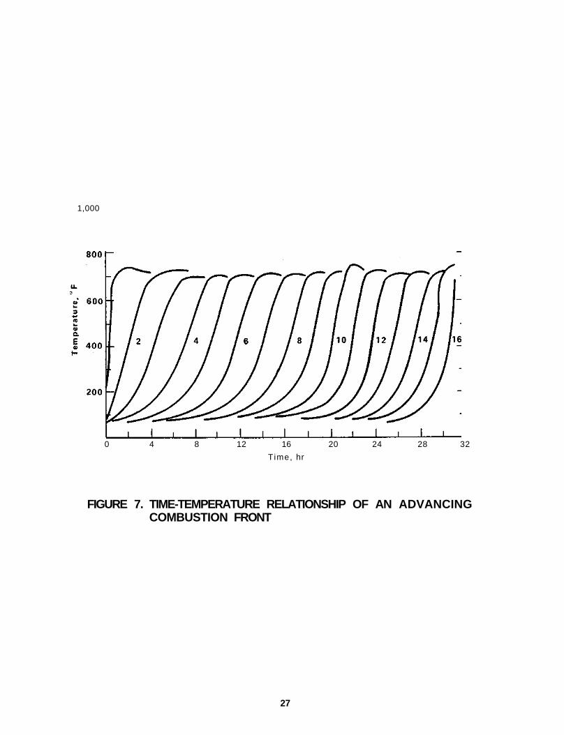
Figure 7 shows the advance of the combustion zone during a typical run as it was recorded by a multipoint temperature recorder. The curves show temperatures measured by each of the 16 thermocouples placed at the center of the tar sand pack and spaced 3 inches apart. The curves are numbered from the top to the bottom of the tube, which was the direction of travel of the burning front. As indicated by each thermocouple, the temperature rose slowly at first as heat was conducted through the tar sand ahead of the burning front. Then the temperature increased more rapidly and reached a maximum as the burning front neared and passed the thermocouple position. With passage of the burning front, combustion ceased because all available oxygen had been consumed. For this particular experiment shown in Figure 7, air flux was 30 scf/hr ft2 and the average peak temperature was 725 °F.
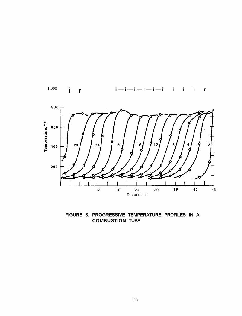
Figure 8 shows the same temperature data replotted as a function of distance from the air-inlet end of the combustion tube with time. The distance of zero corresponds with the bottom of the tube, where air injection occurred. The combustion front moved from right to left. About two hours after ignition, the temperature profile had assumed a shape that remained essentially constant as the combustion front moved through the bed. The shape of the temperature profile Is a function of the rate of air injection. Higher air rates produce higher peak temperatures and steeper temperature gradients, and conversely, lower air rates produce lower temperatures and the temperature profile is spread wider.
Figure 9 is a plot of average peak temperature versus air flux for various combustion experiments. The values indicated by circles were obtained from combustion experiments with Asphalt Ridge tar sand, and the triangles represent P.R. Spring tar sand data. For comparison, the line shows the published data of Reed, et al (5). Temperature data from several tar sand sources were used in constructing this curve.
Figure 10 shows the relationship between combustion front velocity and air flux. Again data from Reed, et al (5) are shown as the straight line for comparison. Velocity of the combustion front is affected to a greater extent than peak temperature by heat loses from, or net heat input to, the combustion tube. Heat loss reduces combustion front velocity, while excess heat input (by the external heaters) increases front velocity. The effect of heat loss and excess heat input on peak temperature is not nearly as pronounced as that on combustion front velocity. Also, variation in thermal properties of the tar sand, such as thermal conductivity and heat capacity, have a greater effect on front velocity than on peak temperature. The data point that is farthest from the curve is from a run in which there was an excess of heat input as a result of improper adjustment of the heater controllers. Similarity of peak temperatures and burning front velocities from different tar sand sources indicates that thermal properties and oxidation rates do not differ significantly for the various tar sand deposits represented.
Oil recovery from the tube combustion experiments is shown in Figure 11. The fraction by weight of the original bitumen content that was recovered by reverse combustion is plotted against air flux. Above approximately 35 scf/hr ft2, the recovery decreases slowly with an increase in air flux because a greater fraction of the bitumen is burned at higher air rates. Below 35 scf/hr ft2, recovery decreases rapidly with decreasing air flux
26
1,000
0 4 8 12 16 20 24 28 32
Time, hr
FIGURE 7. TIME-TEMPERATURE RELATIONSHIP OF AN ADVANCING COMBUSTION FRONT
27
1,000 i r i — i — i — i — i — i i i i r
800 —
12 18 24 30 Distance, in
48
FIGURE 8. PROGRESSIVE TEMPERATURE PROFILES IN A COMBUSTION TUBE
28
1,100
9 0 0
3 +•" 10
a E
•D
m
7 0 0
5 0 0
^ Asphalt Ridge
O P.R. Spring
3 0 0
20 4 0 60 80
Air F lux , scf/hr f t 2
100
FIGURE 9. AIR FLUX VS. PEAK BED TEMPERATURE
29
0.24
.20
I .16 >
o u. c .12 o 3
E o o .08
.04
tk Asphalt R idge
O PR- Spring
20 40 60 80
Air F lux, scf/hr f t 2
100
FIGURE 10. AIR FLUX VS. COMBUSTION FRONT VELOCITY
30
c 0) E 3
O
c
"IZ
o 65
0) > o u
Oi.
0.8
.6
.4
O P.R. Spring
hk Asphalt Ridge
20 40 60 80
A i r Flux, s c f / h r f t 2
100
FIGURE 11. AIR FLUX VS. BITUMEN RECOVERY
31
because at the lower temperature thermal cracking and vaporization of the bitumen are inefficient. At lower air rates some oil is left in the sand. Forward combustion occurs automatically if air injection is continued after the reverse combustion front reaches the air-inlet end of the combustion tube. In forward combustion, coke is burned and any remaining hydrocarbons are vaporized and driven ahead of the combustion front, which now moves in the direction of air flow.
The upper solid curve in Figure 11 is the sum of recoveries from both reverse and forward combustion. Again the dashed curves are reproduced from the paper by Reed, et al (5). The circles represent LETC experimental results of forward combustion following reverse combustion. The lower dashed curve represents recovery from reverse combustion alone. For air fluxes greater than 35 scf/hr ft2, no additional oil is recovered by forward combustion (after reverse combustion). Oil recovery data for the Asphalt Ridge tar sand are in good agreement with the published curve, and the P.R. Spring data show a similar relationship, but with lower recovery values. Maximum oil recovery from the P.R. Spring tar sand approaches 45 wt % of the original bitumen. While the Asphalt Ridge data, which is in agreement with the upper dashed curve, indicates about 50 wt % recovery. There are differences in recovery that may result from the lower oil saturation in the P.R. Spring tar sand, which is approximately 10.5 wt % bitumen, while that in the Asphalt Ridge tar sand is about 12 to 13 wt %.
As evident in Figure 11, the optimum air flux was In the range of 35-40 scf/hr ft where the highest oil recovery occurs. At this optimum air flux, 13,000 scf of injected air was required per barrel of oil produced from the Asphalt Ridge tar sand, compared to 20,000 scf/bbl for the P.R. Spring tar sand. Approximately 10% of the bitumen was burned during reverse combustion. From the Asphalt Ridge samples, 50% of the bitumen was recovered, 40% was left as coke in the sand and 10% was burned.
The oil recovered was a product of thermal cracking of the bitumen and had a gravity of 22.5-23 °API and was of better quality than the original 10 °API bitumen. Sulfur was reduced from 0.5 to 0.02 wt % with about 95% of the sulfur left in the coke on the sand. Water from both vaporized interstitial water and water of combustion amounted to about one-third of the total produced liquids. Analyses of the produced gases showed that all the oxygen in the injected air was consumed in the reverse combustion process. Small amounts of hydrogen, methane, and ethane were detected in the gas from higher temperature runs.
Land (3) has attempted to model the results of some reverse combustion experiments and a brief description of his modeling efforts and results are presented below.
Mathematical analysis of reverse combustion has been restricted to the treatment of temperature and oxygen concentration in a linear system. A fluid flow equation can be written, but this must include the flow of hydrocarbon vapors resulting from thermal cracking. The process of thermal cracking is not well enough understood to be expressed mathematically. In the absence of a cracking equation, the only useful equations are the equations of continuity of heat and oxygen. Berry and Parrish (6) and Warren, Reed and Price (7) have presented these equations. The development that follows is similar to that of both papers.
32
In the absence of heat loss, temperature varies in only one dimension in a combustion tube. For this linear system, the equation of continuity of heat can be written as
3x at *' (D
where Q is the thermal flux due to conduction and convection, Btu/hr ft2; H is the heat content per unit volume, Btu/ft3; Q is the rate of heat generation, Btu/hr ft3; x is the distance in feet taken positive in the direction of air flow; and t is time in hours. Heat conduction is expressed by Fourier's law as
3T q , = -K c o n d 35F ' (2)
where K is the thermal conductivity of the tar sand, Btu/hr ft °F, and T is temperature, °F. Thermal flux by convection is
Q = Y uC T, (3) conv g g
where y is the specific weight of gas, lb/ft3; u is the gas velocity, ft/hr; §nd C is the specific heat of gas, Btu/lb °F. Heat content per unit volume fs the sum of the heat contents of gas and the tar sand and is expressed as
H = (y <}> C +Y C ) T, (4) v'gYg g 'm m'
where <f> is the gas-filled porosity (considering the bitumen to be part of the rocK matrix), fraction of the bulk volume; y is the specific weight of the rock-tar matrix, lb/ft3; and C is the heat capacity of the matrix, Btu/lb °F. The rate of heat generation per unit volume is
0 = <(> hR(c,T), (5)
where h is the heat liberated per unit weight of oxygen consumed, Btu/lb and R(c,T) is the specific reaction rate of the oxygen, lb/hr.
The specific reaction rate is a function of temperature and oxygen concentration, c. Oxygen concentration can be expressed as a fraction of the oxygen concentration of ordinary air.
To arrive at equation (6), the following assumptions have been made:
1. At any time and at any point in the system, the gases, hydrocarbons, and rock are all at the same temperature.
33
2. Heat conduction through the gas is negligible.
3. The rate of heat generation is proportional to the rate of oxygen consumption.
A continuity equation for oxygen, analogous to equation (1), contains the terms: The rate of change of oxygen mass with distance, the time rate of oxygen accumulation, and the rate of depletion of oxygen by reaction. This equation can be written as
3 8 •jp(YaucCo) + g-^gyacCo) + +gR(c,T) = 0 , . x
where C is the weight fraction of oxygen in ordinary air, and y is the specific weight of air, lb/ft3. As C is a constant, equation (7) Decomes
3 t N + 3 /x % + *g R(c,T) = 0. —(yauc) ^rOgyac) c (8)
The rate of reaction of oxygen with the bitumen can be expressed as an Arrhenius equation:
,,/ mx . n -B(T+460) ,„N R(c,T) = Ace (9)
The exponent, n, indicates the order of the reaction with respect to oxygen concentration. A and B are constants. In using equation (9) the assumption is made that there is always an excess of fuel and that the reaction is independent of the quantity of fuel present.
To describe mathematically the temperature and oxygen distributions in space and time during reverse combustion in a linear system, it is necessary to solve equations (6) and (8), making use of equation (9).
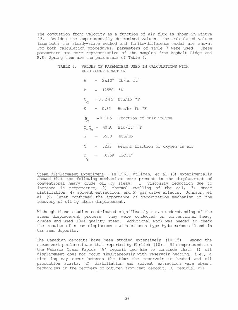
Results of the calculations using both a steady-state method and a finite-difference model show good agreement with laboratory data (3). Peak temperature as a function of air flux obtained from the two mathematical procedures is practically identical. This is true using the parameters of Table 6 and of Table 7 in the calculations. The fact that the peak temperatures resulting from the use of the parameters of both tables are similar, is explained by the previous findings that the order of the reaction and the heat capacity per unit volume have little effect on peak temperature.
Figure 12 illustrates the agreement between calculated peak temperatures and the experimental values. Peak temperatures calculated from both the steady-state method and the finite-difference model are shown, and deviation is believed to be within the range of experimental error.
The combustion front velocities calculated using the same set of parameters are in agreement for the two methods of calculation. Using the parameters of Table 7, the calculated values show better agreement than the combustion front velocities from calculations using parameters from Table 6.
34
1000
800
LL
a 600
0)
a E " 400
200
I I
-
I I
I ' I
O ^
o
I I I
I I I I
Laboratory Data
Steady State
Finite Difference
I I I I
-
-
20 40 60 80 100 Air F lux , scf/hr f t
FIGURE 12. PEAK TEMPERATURES VS. AIR FLUX BY THREE DIFFERENT METHODS
35
The combustion front velocity as a function of air flux is shown in Figure 13. Besides the experimentally determined values, the calculated values from both the steady-state method and finite-difference model are shown. For both calculation procedures, parameters of Table 7 were used. These parameters are more representative of the samples from Asphalt Ridge and P.R. Spring than are the parameters of Table 6.
TABLE 6. VALUES OF PARAMETERS USED IN CALCULATIONS WITH ZERO ORDER REACTION
A = 2xl06 Ib/hr ft3
B = 12550 °R
C =0.245 Btu/lb °F g
K = 0.85 Btu/hr ft °F
(j> =0.15 Fraction of bulk volume g
Y C = 40.A Btu/ft3 °F m m
h = 5550 Btu/lb
C = .233 Weight fraction of oxygen in air
T = .0769 lb/ft3 g
Steam Displacement Experiment - In 1961, Willman, et al (8) experimentally showed that the following mechanisms were present in the displacement of conventional heavy crude oil by steam: 1) viscosity reduction due to increase in temperature, 2) thermal swelling of the oil, 3) steam distillation, 4) solvent extraction, and 5) gas drive effects. Johnson, et al (9) later confirmed the importance of vaporization mechanism in the recovery of oil by steam displacement.
Although these studies contributed significantly to an understanding of the steam displacement process, they were conducted on conventional heavy crudes and used 100% quality steam. Additional work was needed to check the results of steam displacement with bitumen type hydrocarbons found in tar sand deposits.
The Canadian deposits have been studied extensively (10-15). Among the steam work performed was that reported by Ehrlich (10). His experiments on the Wabasca Orand Rapids "A" deposit led him to conclude that: 1) oil displacement does not occur simultaneously with reservoir heating, i.e., a time lag may occur between the time the reservoir is heated and oil production starts, 2) distillation and solvent extraction were absent mechanisms in the recovery of bitumen from that deposit, 3) residual oil
36
0.25
"£ .20 -
u _o > c o
c o
3
E o o
.10
.00
-
—
-
-
-
_
- '
-
I I I
o /
o/
I I I
I I I I I I
0 S^ —
x° V -
O Laboratory data —
— Steady State _
£x Finite Difference
I I I I I I 20 40 60 80 100
Air F lux , scf/hr f r
FIGURE 13. COMBUSTION FRONT VELOCITY VS. AIR FLUX BY THREE DIFFERENT METHODS
37
TABLE 7. VALUES OF PARAMETERS USED IN CALCULATIONS WITH FIRST ORDER REACTION
A
B
C g
K
•« Y C m m
h
C o
Y„
ss
=
=
=
=
=
=
=
=
1.96x1
12500
0 . 2 4 5
0 . 8 5
0 . 2 6
3 5 . 0
5550
•0.233
0 .0769
,6
g
°R
Btu/lb °F
Btu/hr ft °F
Fraction of bulk volume
Btu/ft3 °F
Btu/lb
Weight fraction of oxygen in air
lb/ft3
saturation was 20% regardless of initial oil saturation, 4) area] sweep efficiency was high due to low steam mobility, 5) steam override would eventually occur, lowering the vertical sweep efficiency, and 6) presence of bottom water would increase oil recovery.
Watts (16) and Watts, et al (17) reported on laboratory steam displacement tests conducted on Utah tar sands, and a review of their work is discussed below.
The experiments were run in a 3.25-inch I.D. stainless steel tube, 32.12.5 inches in length. The tube was surrounded by an insulated jacket containing five heaters that could be used either to heat the tube or act as an adiabatic shield. Five thermocouples positioned opposite the heaters in an axially concentric thermowell provided the reference temperatures for operation in the adiabatic mode. Figure 14 shows a schematic of the system. The tube and its associated thermocouples, heaters, and controllers are represented as "core holder". The boiler was capable of supplying steam at a constant rate and quality at pressures of up to 500 psig.
An experiment was initiated by first packing the tube with loose tar sand material with the thermowell in place and the heaters set at about 170 °F to facilitate packing. The material charged was weighed to within an accuracy of about 0.2%. Once packing was complete, the tube was assembled and put into the adiabatic mode. The boiler was started and steam was fed into a bypass line until it reached desired operating conditions. Steam quality and rate were measured by diverting the injection steam from the tube into a calorimeter type quality measuring device.
Once the quality and rate were adjusted to the desired values, stem flow was started into the tube. Temperatures at all thermocouples and the inlet line were continuously recorded. The downstream valve was opened every ten
38
Feed Water Water
Softener Boilei
•n^»
nlet Pressure
° " 1
Feed Pump
fi* Inlet Steam
Valve -H8K-
Pressure G a u g e d
•• ~ • • ••••
-Tar Sand
Steam Injection Line
Core Holder
Outlet V a l v e ^ Water
Cooled
Outlet Pressure " 0 Gauge
M a i n Stream Va lve
Pressure Gauge
- L _ _ S ) V a l ve
Condenser Collection
Vessel
Steam Quality and Flow Measuring
Device /
/ • Thermometer
FIGURE 14. THE WATTS LABORATORY STEAM INJECTION SYSTEM
minutes to collect production. This precluded true steady-state operation of the tube but was necessary to maintain the desired steam pressure (and temperature) , as the permeability was so high that only about a 10 psi pressure drop could be achieved across the system. Samples were collected every thirty minutes and the production volumes measured. Some samples were tested further for gravity and composition to ascertain variation during the run.
When a run was made using nitrogen as the injected fluid, the heaters were manually controlled so as to simulate the temperature history of a steam run using the same temperature and gas flow rate. Injection rates were measured with a nitrogen mass flowmeter. The rest of the experiment closely followed the procedure of the steam runs.
Two runs were made with hot water injection. The apparatus for this experiment is shown in Figure 15. The core holder was a 2.375-inch I.D. x 12.0-inch long tube with three axially parallel guard heaters, which were operated manually to simulate an adiabatic shield. This arrangement did not permit longitudinal temperature gradients but this did not appear to be detrimental to the results. Nitrogen provided the desired pressure to the system and water was heated to the desired operating temperature in the heat tape section of the system.
A total of eleven experiments were conducted, and Table 8 summarizes the run conditions and oil recovery results. All runs reported were made at saturated steam conditions. The maximum saturated steam temperature of 450 °F was determined by an anticipated maximum bottom hole injection pressure (at field conditions) of 500 psi. Other temperatures were chosen to provide a range for comparison. Bun 3 was a repeat of run 2 with the exception that it lasted longer. The hot water experiments (runs 8 and 10) were kept about 100 psi above saturation pressure to prevent flashing of the hot water.
TABLE 8. EXPERIMENTAL CONDITIONS, WATTS HOT WATER-FLOOD TESTS
Steam Water Run Bitumen Temp, Flowrate, Quality, Duration, Recovery,
FIGURE 15. THE WATTS LABORATORY HOT WATER FLOOD SYSTEM
Typical experimental results are portrayed by the temperature profiles in Figure 16 and oil recovery curves in Figure 17 for run 3. In general, no oil production occurred until after steam breakthrough, at which point an oil bank arrived. After that time, the temperature in the tube remained constant at injection steam temperature for the duration of the run and oil production declined. Because oil production occurred before steam breakthrough, it indicates that bitumen must be thoroughly heated before it becomes mobile. It also suggests that the effect of temperature profiles ahead of the front is minimal, thereby assuring that the manual operation of the heaters during nitrogen and hot water runs did not significantly affect the results of those runs.
Oil samples were collected at several points during some of the runs and were subjected to simulated distillation analyses to determine if the composition of the product changed throughout the process. Table 9 shows the results of the samples analyzed from run 3. As can be seen, initially a heavy oil was produced followed by an increasingly lighter grade of product. This behavior was typical for all runs except the hot waterflood runs, as typified by run 8, Table 10, where only a heavy oil was produced during the run. The nitrogen runs produced less of the heavy oil component than the steam runs, as exemplified by run 7, Table 11. For reference, the native bitumen contains about 59% residue boiling above 1000 °F.
TABLE 9. SIMULATED DISTILLATION DATA FROM RUN 3
Time into Run, Oil with Boiling Oil with Boiling
hr Point >1000 °F, % Point of 601-700 °F, %
2.75 55.8 5.9
8.0 29.8 21.2
16.0 23.2 32.0
TABLE 10. SIMULATED DISTILLATION DATA FROM RUN 8
Time into Run, Oil with Boiling hr Point >1000 °F, %
1.5 57.2
2.5 58.1
4.5 56.7
42
400
300
5 200
Q.
E
100
i r i 1 r
\ \
V \ \
•v.. \
— 0 Minutes 60 Minutes
— 10 Minutes 100 Minutes
— 40 Minutes - 120 Minutes _L
6 9 12 15 18 21 Distance f rom Steam Inlet, in
24 27
FIGURE 16. TEMPERATURE PROFILES DURING STEAM INJECTION, WATTS RUN NO. 3
43
FIGURE 17. OIL RECOVERY VS. TIME, WATTS RUN NO. 3
44
TABLE 11. SIMULATED DISTILLATION DATA FROM RUN 7 (NITROGEN)
Time into Run, hr
Oil with Boiling Point >1000 °F, %
Oil with Boiling Point of 601-700 °F, %
4.5
5.5
6.5
7.5
23.2
9.1
10.9
13.0
4.4
18.8
30.7
54.6
Because a steam drive encompasses a hot water-flood, the mechanisms associated with a hot water-flood are also part of the steam drive. The Increased "solvent enrichment" is believed to account for the remaining 5-6% oil recovery in run 2. It also explains the sequence of production observed in Table 12. As the light oil vaporizes and recondenses, the greatest percentage of it condenses near the outlet end of the tube, thereby lowering the viscosity of this oil enough to allow it to be produced when combined with the thermal effects on viscosity reduction. Heavier oil was the first to be produced from the core.
TABLE 12. OIL SATURATION IN NORTHWEST ASPHALT RIDGE TAR SAND AFTER STEAM-FLOOD
Residua] Oil Saturation Residual Oil Saturation Oil in in Top of Core, in Bottom of Core, Original Sample
wt % wt % Run No
2
3
4
5
6
7 (N ?)
8 (Hot H ? 0)
wt %
10 .2
9 . 6
8 . 8
9 . 3
9 . 9
10 .4
9 . 8
7.9
8.5
7.4
6.2
8.3
11.4
6.6
12.1
11.2
11.1
11.4
11.7
12.5
11.6
If this concept is accurate, it would follow that more oil should have been produced from near the outlet than from near the inlet. This hypothesis was tested by removing samples of residual material from near the inlet and outlet ends of the core after the runs and determining residual saturation.
45
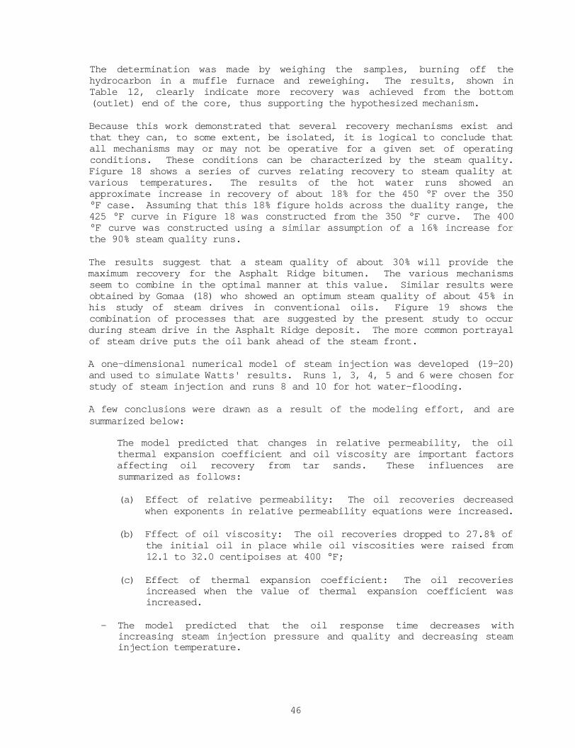
The determination was made by weighing the samples, burning off the hydrocarbon in a muffle furnace and reweighing. The results, shown in Table 12, clearly indicate more recovery was achieved from the bottom (outlet) end of the core, thus supporting the hypothesized mechanism.
Because this work demonstrated that several recovery mechanisms exist and that they can, to some extent, be isolated, it is logical to conclude that all mechanisms may or may not be operative for a given set of operating conditions. These conditions can be characterized by the steam quality. Figure 18 shows a series of curves relating recovery to steam quality at various temperatures. The results of the hot water runs showed an approximate increase in recovery of about 18% for the 450 °F over the 350 °F case. Assuming that this 18% figure holds across the duality range, the 425 °F curve in Figure 18 was constructed from the 350 °F curve. The 400 °F curve was constructed using a similar assumption of a 16% increase for the 90% steam quality runs.
The results suggest that a steam quality of about 30% will provide the maximum recovery for the Asphalt Ridge bitumen. The various mechanisms seem to combine in the optimal manner at this value. Similar results were obtained by Gomaa (18) who showed an optimum steam quality of about 45% in his study of steam drives in conventional oils. Figure 19 shows the combination of processes that are suggested by the present study to occur during steam drive in the Asphalt Ridge deposit. The more common portrayal of steam drive puts the oil bank ahead of the steam front.
A one-dimensional numerical model of steam injection was developed (19-20) and used to simulate Watts' results. Runs 1, 3, 4, 5 and 6 were chosen for study of steam injection and runs 8 and 10 for hot water-flooding.
A few conclusions were drawn as a result of the modeling effort, and are summarized below:
The model predicted that changes in relative permeability, the oil thermal expansion coefficient and oil viscosity are important factors affecting oil recovery from tar sands. These influences are summarized as follows:
(a) Effect of relative permeability: The oil recoveries decreased when exponents in relative permeability equations were increased.
(b) Fffect of oil viscosity: The oil recoveries dropped to 27.8% of the initial oil in place while oil viscosities were raised from 12.1 to 32.0 centipoises at 400 °F;
(c) Effect of thermal expansion coefficient: The oil recoveries increased when the value of thermal expansion coefficient was increased.
- The model predicted that the oil response time decreases with increasing steam injection pressure and quality and decreasing steam injection temperature.
46
100
80
60 -
a. - 40 O
- ] 1 r
• Calculated Point
O 350°F
A 400°F
O 425°F
40 60
Steam Qual i ty, %
80 100
FIGURE 18. RECOVERY VS. STEAAA QUALITY FOR VARIOUS WATTS RUNS
47
Overburden
a>
s c 0
o
c
E (0 a) +•» CO
\
\o . . \ 'Bank!
Residual 1 Steam
/
Hot Water
Flood
Oil / F ront
/
1
Vapor iza t ion
I
/ Virgin
Cold / Reservoir
Water /
Flood J
.
Condensation (Dist i l lat ion) / Enr ichment
/ Viscosity Reduct ion /
_ 0)
5 c o +•» u 3
•D O
> a.
Underburden
FIGURE 19. SCHEMATIC OF THE STEAM FLOOD PROCESS IN ASPHALT RIDGE TAR SAND
48
Ip (21) continued Watts' work on Asphalt Ridge samples by studying the effect of co-injection of steam and inert gases or steam and air. Steam injection is an effective recovery technique with the unique heat-carrying capacity of steam resulting in an improved mobility ratio over that of air injection; however, it does suffer a restricted operating temperature limit. In situ combustion does not suffer from this temperature restriction, but its overall performance as an efficient recovery process is handicapped by the poor mobility ratio of a gas drive, especially for recovery of viscous oils where fingering is common. Consequently, it appears that a combination of steam injection and in situ combustion in some fashion would eliminate some of the problems observed when these methods are used independently. Drive mechanisms of this kind would be complex because oxidation reactions are present. Any attempt to study this process should be accompanied by a study of the drive mechanisms of the process when no oxidation is involved. This would simplify the effort to isolate the mechanisms involved.
Nitrogen and carbon dioxide were the non-reactive gases used by Ip in conjunction with steam, while air was the reactive gas used. Twenty-one runs were conducted in the apparatus used for Watts' study. The purpose of this series of runs was to compare the performance of a steam/coinjectant process with a straight steam displacement process and to describe the factors that determine the performance and the mechanisms that are believed to contribute to the effectiveness of the process.
Because of the complex nature of recovery mechanisms, which may involve steam distillation, thermal expansion of fluids, reduction of fluid viscosity, gas drive, and miscible displacement, every effort was made to isolate as many process variables as possible. First, the operating temperature and pressure for all the runs were chosen to be 447 °F and 400 psi, respectively, or values as close to those as possible. Second, the steam flow rate for all the runs was set at or near 2.75 lb/hr. Third, gas injection rates were either 0.1 scf/min or 0.5 scf/min for all non-reactive gas concurrent runs and 0.05 scf/min for all reactive gas (air) runs.
The following conclusions were made by Tp (December 1980) in his study:
Tn laboratory experiments, the addition of non-reactive gases to steam injection can only produce slightly improved oil recovery performance over steam alone.
- In a steam drive with co-injected non-reactive gas, higher gas injection rates would result in slightly higher oil recovery during the period when gas drive dominates the additional recovery mechanism, but would perform no better than lower gas injection rates during the period when oil vaporization dominates any additional recovery mechanisms. ,
- Both the concurrent and altering mode in a steam drive with non-reactive gas injectants are equally effective in oil recovery in tar sand, based on the same volume of non-reactive gas injected.
- Spontaneous ignition may occur in a steam flooded tar sand pack when the pack is in contact with an oxygen-containing gas for a prolonged period.
49
- It is more efficient in displacement to recover oil in tar sand by first heating the oil sand to high temperature with air injection, and then displacing it in the heated zone by a steam-flood.
- An air/steam drive, either in the alternating or concurrent mode, is more effective in recovering oil from tar sand than any kind of non-reactive gas with steam or steam-only drives.
Shirazi (20) later extended Ip's work with several experimental runs using co-injection of ambient air and steam. Conclusions made by Shirazi for his experimental conditions where combustion did not occur are the following:
- Co-injection of steam and ambient temperature air into a tar sand pack will yield a higher percentage of oil recovery than either one injected alone if less than 60 volume percent of the total fluids injected is air.
- Maximum oil recovery occurred when ambient air and steam were co-injected in approximately equal volumes (the volumetric air/steam ratio was close to 1).
- Simultaneous injection of ambient air and steam did not show a significant difference compared to alternating injection of steam and air in these experiments.
- Low temperature oxidation occurred during co-injection of steam and ambient temperature air.
In situ combustion is probable in an alternating injection of steam and ambient air, particularly when the air/steam ratio (by volume) is close to 1.
- A high percentage air (over 60 volume percent of total) in a co-injection process causes a lower oil recovery.
50
REFERENCES
"Industry Gearing up for Assualt on Athabasca Tar Sands." Oi] Gas J. 72(5), 1974, pp. 85-90.
Trantham, J. C. and J. W. Marx. "Bellamy Field Tests: Oil from Tar by Counterflow Underground Burning." Trans. AIME (1966) 237; pp. 109-115.
Land C. S. "Reverse Combustion in Tar Sands." Ph.D. Dissertation, Univ. of Wyoming, August 1974.
Land C. S., F. M. Carlson, and C. Q, Cupps. "Laboratory Investigations of Reverse Combustion in Two Utah Tar Sands." U.S. Energy Research and Development Administration-Laramie Energy Research Center Report of Investigation RI-75/2. Oak Ridge, TN, 1975, 29 pp.
Reed, R. R. , D. W. Reed, and J. H. Tracht. "Experimental Aspects of Reverse Combustion in Tar Sands." Trans. Petrol. AIME 219, pp. 99-108.
Berry, V. J., Jr., and 0. R. Parrish. "Theoretical Analysis of Heat Flow in Reverse Combustion." Trans., AIME (1960) 219, pp. 125.
Warren, J. E., R. L. Reed, and H. S. Price. "Theoretical Considerations of Reverse Combustion in Tar Sands." Trans., AIME (1960) 219, pp. 109.
Willman, B. T., V. V. Valleroy, G. W. Runberg, A. J. Cornelius, and L. W. Powers. "Laboratory Studies of Recovery by Steam Injection." J. Pet. Tech., July 1961, pp. 681-693.
Johnson, F. S., C. J. Walker and A. F. Bayazeed. "Oil Vaporization During Steamflooding." Trans. AIME (1971) 251, pp. 731-742.
Ehrlich, R. "Laboratory Investigation of Steam Displacement into the Wabasca Grand Rapids "A" Sand." Oil Sands of Canada-Venezuela, 1977. D. A. Redford and A. G. Winestock, eds., CIm Spec. Vol. 17, pp. 364-387.
Farouq Ali, S. M. "Physical Modeling of In Situ Recovery Methods for Oil Sands." Oil Sands of Canada-Venezuela, 1977 op. cit., pp. 319-327.
Flock, D. L. and J. Lee. "An Experimental Investigation of Steam Displacement of a Medium Gravity Crude Oil." Oil Sands of Canada-Venezuela, 1977, op. cit., pp. 386-394.
Harris, M. C. and J. C. Sobkowicz. "Engineering Behavior of Oil Sand." Oil Sands of Canada-Venezuela, 1977, op. cit., pp. 270-279.
Prats, M. "Peace River Steam Drive Scaled Model Experiments." Oil Sands of Canada-Venezauela, 1977, op. cit., pp. 346-363.
51
Redford, D. A., D. L. Flock, E. Peters, and J. Lee. "Laboratory Model Flow Test Systems of In Situ Recovery from Alberta Oil Sands." Ann. Meeting, Canadian Chemical Society, Montreal, Can. (1976).
Watts, K. G. "Investigation of the Steamflood Mechanism for the Asphalt Ridge Tar Sands Deposit, Utah." M. S. Thesis, Univ. of Wyoming, December 1979.
Watts, K. G., H. L. Hutchinson, L. A. Johnson, R. V. Barbour and K. P. Thomas. "Experimental Investigation of the Steam Drive Process for the Asphalt Ridge Tar Sands Deposit, Utah." SPE 11161 presented at 57th Annual Fall Meeting of the SPE if AIME, New Orleans, LA, September 26-29, 1982.
Gomaa, E. E. "Correlations for Predicting Oil Recovery by Steamflood." J. Pet. Tech., February 1980, pp. 325-332.
Chen, C. S. "One-Dimensional Modeling of Steam Injection in Tar Sands." M.S. Thesis, Univ. of Wyoming, December 1982.
Chen, C. S. and H. L. Hutchinson. "One-Dimensional Modeling of Steam Injection in Tar Sands." SPE 11849, presented at 1983 SPE Rocky Mountain Regional Meeting, Salt Lake City, Utah, May 23-25, 1983.
Ip, D. T. "Laboratory Studies of Oil Recovery by Steam Injection with Gas Co-Injections in Tar Sand." M.S. Thesis, Univ. of Wyoming, December 1980.
Shirazi, M. R. "Experimental Studies on Tar Sand Retorting by Co-Injection of Steam and Air." M.S. Thesis, Unive. of Wyoming, December 1982.
52
GEOLOGICAL SITE EVALUATION
The geological evaluation of a 26-acre LETC tar sand site in Utah has included three techniques: geology, high resolution seismic survey, and well logging. At the Vernal tar sand field experiment site, 80 wells were drilled and cores were taken and analyzed from most wells. The total core data from the site has not been included in this report, however, average pattern core values have been discussed in the geology category and also in the sections dealing with individual tests. Core analyses values have also been plotted for comparison with log-derived values in the well logging category.
Geology - The Northwest Asphalt Ridge tar sand deposit (1) was the site selected by LETC for in situ field experimentation. Asphalt Ridge is a 15-mile-long northwest trending hogback on the northeastern margin of the Uintah Basin; a structural and topographic Tertiary basin (2). The northwest end of the ridge has been downdropped by a series of major northeast trending faults. One fault has approximately 900 ft of displacement, consequently lowering significantly the northwest portion of the Asphalt Ridge. This downdip block, a monocline dipping southwest, has been named the Northwest Asphalt Ridge deposit. LETC has conducted three field tests on 10 acres within that deposit. Figure 20 shows a location map of the test site.
Oil-impregnated strata occur at both the Asphalt Ridge and Northwest Asphalt Ridge deposits. Regionally, the late Cretaceous Mesaverde Formation is unconformably overlain by the Eocene Duchesne River Formation (see Figure 21). At Asphalt Ridge, the Mesaverde Formation dips from 12-28° southwest, while the Duchesne River Formation is less steep, dipping about 5-20°. At Asphalt Ridge, oil-impregnated strata are exposed along the entire strike of the Ridge. About 113 ft of oil-impregnated Rimrock Member of the Mesaverde Formation is exposed at the northwest end of the Ridge, while 190 ft of oil-bearing Duchesne River Formation and Rimrock Sandstone are exposed at the Uintah County asphalt quarry (3). The only exposures of oil-impregnated strata at Northwest Asphalt Ridge are just west of the fault separating it from Asphalt Ridge. The oil-impregnated Mesaverde Formation occurs in sporadic outcrops for about 3,000 ft, approximately 1/4 mile northeast of the test site. The Mesaverde and Duchesne River Formations are also saturated at the Northwest Asphalt Ridge deposit. These beds dip to the southwest between 19 and 45°.
Two major lithographic units, the Duchesne River Formation and the Rimrock Sandstone, have been cored at the LETC field site (see Figures 22 and 23). The Oligocene Duchesne River Formation is of continental origin and is characterized by interbedded sandstone, siltstone, shale and large angular conglomerate. The Uintah Mountains to the north were the source for some of the coarser sediments. The conglomerate is particularly prevalent at the bottom of the formation and is utilized as a marker bed. The formation contains varying amounts of oil saturation and rests with angular unconformity on the Cretaceous Mesaverde Formation. This Formation is divided into three members (youngest to oldest): the Rimrock Sandstone, the Mesaverde Shale (or Mancos Shale) and the Asphalt Ridge Sandstone; all are of marine origin. Most of the drilling and coring at the field site was completed through the Rimrock Sandstone.
53
Legend
Oi l - Impregnated Sandstone Exposure
D # U M a j o r Normal Fault
(££) Quarry
• Wel l Location
Cross Section Location
FIGURE 20. LOCATION MAP OF THE LETC TAR SAND FIELD SITE, ASPHALT RIDGE AND NORTHWEST ASPHALT RIDGE, UTAH
SW
+6000
-4000
Carter Oil No.l Knudsen
Elev. 5393 D.F.
Home Oi l -West Venture
No. 1 Elev. Approx. 5500'
NE
Asphalt Ridge
Kayser, 1966
Geologic Age
O - Oligocene E - Eocene P - Paleocene C - Cretaceous
Scale, miles
Vi 1
FIGURE 21. GEOLOGIC CROSS SECTION OF THE ASPHALT RIDGE AREA AND SOME CORE LOCATIONS, UINTAH COUNTY, UTAH
Elevation, ft
5950—
5900 — -. 9 •*>?:••
ps
5800 —
5700-
Detail ^ • • ' r ^ \
5600 — bs^d
5500 —
5400-
5300-
5200 —
Sloe
s ' 9
0 ' .0* . .0 m S!
- -Q
u-y-XJl
Surface Aluvium
Unconformity
"T Rimrock Sandstone
Mesaverde Shale
Asphalt Ridge Sandstone
Shale
Duchesne River
Format ion i
Oligocene
M e s a v e r d e Format ion
i Cretaceous
M a n cos Format ion
i
Cretaceous
m W$ Conglomerate
Shale, Siltstone
Limestone
Sandstone
FIGURE 2 2 . A GENERALIZED STRATIGRAPHIC SECTION AT LETC FIELD SITE, UINTAH COUNTY, UTAH
56
450
475
500
o D
CO
_o
CQ
a a>
Q
525
550- i
575-
600-
Unconformity
PPI1 Sandstone
^ra Oil- Impregnated ^ ^ Sandstone
625
6 5 0 - i
675-
3 i V* V. ? * rf. » i *v- i>*^» ( J
Kfc
Lower Zone
FIGURE 23. GENERALIZED LITHOLOGIC SECTION OF RIMROCK SANDSTONE, UINTAH COUNTY, UTAH
57
The major source of tar sand at Northwest Asphalt Ridge is the Rimrock Sandstone. It is a highly saturated, semi-consolidated to consolidated, fine- to medium-grained sandstone with many low saturated claystone, siltstone and shale intervals that vary in thickness from less than 1 inch to more than 10 ft. The sandstone contains 60% chert, 37% quartz and minor accessory minerals (4). It is cemented by calcite and minor authigenic quartz. Continuous tar sand sections without a shale break vary from less than 1 ft to more than 40 ft in thickness. At the site, the entire section appears to increase in thickness toward the southeast from 150 ft to more than 240 ft.
Three tar sand intervals are present within the Rimrock Sandstone. The upper tar sand zone is a fairly continuous, highly saturated interval characterized by low permeabilities and variations in thickness from 10-80 ft across the site. This wide variation is attributed to the erosional unconformity between the Mesaverde Formation and the overlying Duchesne River Formation. The middle tar sand zone, designated the TS-1S zone, is well saturated, permeable and about 50 ft thick. There are shale lenses throughout this zone. The lower zone averages 45 ft in thickness and has high permeability but low oil saturation. Significant shale zones separate the three identified tar sand zones.
Below the Rimrock Sandstone lies a shale zone 70-90 ft thick, referred to as the Mesaverde Shale. Some authors believe it to be an upper tongue of the Mancos Shale (5). The Asphalt Ridge Sandstone, the lower unit of the Mesaverde Formation, lies beneath this shale zone. It is also of marine origin and is easily distinguishable from the Rimrock Sandstone by an abundance of quartz, a small percentage of chert and finer grain size. Average oil saturation is less for the Asphalt Ridge Sandstone than for the Rimrock Sandstone.
The middle tar sand zone of the Rimrock Sandstone was utilized for all field tests conducted by LETC on a 10-acre tract. Reservoir properties of the test zone for each of the three field tests vary across the site. Porosity is fairly consistent, and an average for the site ranged from 26 to 31 percent. However, the average saturated and extracted permeabilities and average water saturation vary randomly.
Extensive faulting has occurred in the Cretaceous Mesaverde Formation at the field site. These small displacement (10-30 ft), high angle faults were difficult to detect during drilling. However, a 6-line seismic survey clearly defined a series of faults trending northwest-southeast. The survey also indicated the presence of a structural basin in the lower part of the Mesaverde Formation southeast of the 10-acre tract. There are probably numerous undetected small displacements, parallel and perpendicular fractures and faults that are generally related to the larger faults.
The origin of oil in the Cretaceous and Oligocene strata was probably the lacustrine Green River Formation oil shales of the Uintah Basin (6) . During tectonic activity the sediments of the Asphalt Ridge area were uplifted in relation to those of the Uintah Basin, allowing the oils in the Eocene sediments to migrate updip along the porous and permeable sandstones near the unconformity (7) . Faulting also contributed to localizing the migrating oils and forming impermeable barriers, thus creating structural
58
traps. Migration of the oil occurred in post-Oligocene time, following deposition of the Duchesne River Formation.
High Resolution Seismic Survey - High resolution seismic data were utilized to investigate the structural configuration of tar sands and related geological units at the LETC Northwest Asphalt Ridge tar sand site (8). The major objective of this study was to map fault patterns to define areas that might be prospective for the drilling of multiple holes. Field data acquisition and processing were directed toward defining shallow structures, less than 1,000 ft deep. Six short seismic lines were "shot" in a grid pattern. Seismic data were acquired using a 48-channel, Texas Instruments DFS V recording system with a vibrator source. The geophone interval was 20 ft and the standard source interval was 40 ft yielding an average horizontal stack of 12-fold throughout the area. The upper sweep frequency of 140 Hz was for the purpose of generating enough high frequency energy to acquire data with sufficient resolution to map shallow units.
The resolution of the seismic method is a function of the geology (i.e., the physical properties of the rocks), the spatial sampling and the frequencies of energy transmitted through the earth. The wavelength of the seismic wave is the scale and it is determined by dividing the velocity by the frequency. For example, if the velocity is 10,000 ft/sec, and the highest frequency traveling through the ground is 100 Hz, then the wavelength is 100 ft. It has been suggested in the literature (9-10) that the resolution is 1/8 to 1/12 of the wavelength. In this example, the resolution would be limited to units at least 8 to 12 ft thick.
Six seismic lines of approximately 1/4 mile each were shot in the study area. These data were useful for defining specific structures, but provided minimum information on the regional structure due to the length of the lines. Complexities in the near-surface area included the presence of conglomerates, lack of water-saturated units, and topography. Unfortunately these constraints, which may limit the resolution, could not be overcome by any cost-effective, conventional seismic approach. The problem might have been solved by deep shot holes, and/or a VSP (vertical seismic profiling) approach.
Seismic Data Processing - Processing was carried out with the specific goal of emphasizing the shallow data. Detailed processing emphasized those processes that are extremely important in the analysis of high resolution data such as static corrections, velocity analysis, etc. The data are generally of good quality, as good as might be expected in such a complex, highly faulted terrain. The resulting interpretation, therefore, has a reasonable degree of confidence placed in it.
Seismic Data Interpretation - The interpretation of seismic data proceeded concurrently with iterative processing. The interpretation presented in this report began with a compilation of data from well logs and these data resulted in two maps. One was a contour map of the top of the upper tar sand (Figure 24) and an isopach map of this interval (Figure 25). The structural map shows a high in the north, plunging to the west-southwest. One must bear in mind that this contour map is based on only a limited number of drill holes that penetrated the entire Rimrock Sandstone. Consequently, seismic interpretation provides more detail of the structure, but should be compatible with this interpretation. The isopach shows that
59
ON
o
Note: Elevations Above Sea Level Scale, ft
0 100 200 400
FIGURE 24. TOP OF RIMROCK TAR SAND CONTOUR MAP
Scale, ft
0 100 200 400
FIGURE 25. UPPER RIMROCK TAR SAND ISOPACH MAP
the maximum thickness for the tar sand is in the structural low in the vicinity of line 2, stations 720 and 740, approximately in the vicinity of well 4P3-B. The genera} trend is a thickening to the south-southwest
Seismic data were used to develop two structure maps. These are contoured on the "yellow" horizon (Figure 26) and the "orange" horizon (Figure ?J). The "yellow" reflector is the first reflector with good continuity that can be traced over the area. The "orange" reflector is picked for the purpose of determining the thickness and general structure in the tar sand section. On some of the sections, the apparent upper tar sand unit is marked. This unit appears to be relatively discontinuous except in areas of maximum tar sand thickness. The lack of continuity may be a function of bitumen saturation with the unit and/or the composition (porosity, clay content, etc.) of the unit. A comparison of the structural map of the "yellow" horizon and the "orange" horizon with the map derived from the well data shows the same basic trends. There is a structural high in the northern portion of the map that plunges to the southwest. However, there are more details evident on the seismic data than are evident on the well data.
Veil Logging - After completion of the two combustion experiments the decision was made to begin supplementing the coring program with more auantitative logging and, if possible, reduce the number of wells cored by relying on log data.
For this study, data were available for eight wells (11). Core and log data were available for comparison on five wells, and three wells had reservoir data derived entirely from logs. These wells were used to conduct a steam-flood experiment and provide reservoir data for the design of a fourth field experiment. Figure 28 is a map of the ?6-acre site locating the eight additional wells under discussion, and Table 13 summarizes the logging procedures used for each well.
For purposes of this study, the Rimrock Sandstone Member has been divided into five zones. These intervals were differentiated based on a combination of drill cuttings, core data, and well log information. In general, three zones are relatively clean tar sand zones while two are shaly or interbedded. The first zone, called the upper tar sand zone, was a fairly continuous, highly saturated tar sand interval. It appeared to vary in thickness from 30 to 85 ft within the site. This variation is caused by an erosional unconformity between the overlying Eocene Duchesne River Formation and the Cretaceous Rimrock Sandstone Member. The second zone, called the interbedded zone, varies in thickness from 35 to 55 ft. This zone is a combination of tar sand and low saturated siltstone intervals, which vary in thickness from a few inches to several feet. The third zone was the LETC tar sand test zone. Part of all of this interval was utilized for the three field experiments conducted at the site. This interval was characterized by acceptable permeability and high oil saturation. Saturation appears to decrease drastically in the downdip direction. The tar sand test zone was about 50 ft thick. The fourth zone, commonly referred to as the shale zone, consisted of 6 to 10 ft of shale or siltstone and was characterized by low permeabilities and low oil saturations. The fifth interval was referred to as the lower tar sand zone and was a 45 to 55 ft thick tar sand interval characterized by low oil
62
ON CO
/
LETC Tar Sand Site Boundary
Scale, ft
Contour Interval = 20/i.sec 0 100 200 400
FIGURE 26. "YELLOW" HORIZON CONTOUR MAP
4>
/
LETC Tar Sand Site Boundary
Scale, ft
Contour Interval = 20/tsec 0 100 200 400
FIGURE 27. "ORANGE" HORIZON CONTOUR MAP
LETC
Original 10 Acre Site
3P3 0 0 3P8 O 311
3P6 O
0 5T1 LETC
Addi t ional 16 Acre Tract
O 4P3B O 4P5
O 5T3
FIGURE 28. SELECTED LETC TAR SAND WELL LOCATIONS, ASPHALT RIDGE AREA, UTAH
65
saturation and high permeability. Part of this zone had been logged and cored in all 8 wells. Unfortunately, log and core data for the entire lower zone were available for only one well (5T3). Figures 29 and 30 are correlations of the area under consideration utilizing gamma ray logs from the eight wells.
TABLE 13. WELL LOGGING AND CORING SUMMARY, NORTHWEST ASPHALT RIDGE
Well No Logging Suite Well Cored
3PE Gamma, Compensated Neutron, Density, SP, Induction, Caliper, Sonic
Yes
3P6
4P3B
4P5
Gamma, Compensated Neutron, Density, SP, Induction, Caliper, Sonic
5T1 Gamma, Sidewall Neutron, Density, SP, Induction, Caliper, Differential Temperature
Yes
5T3
311
3P8
Gamma, Sidewall Neutron, Density, SP, Induction, Caliper, Sonic
Gamma, Carbon/Oxygen
Gamma, Carbon/Oxygen
Yes
No
No
Because sufficient logging data are lacking on U.S. tar sand deposits, particularly in Utah, two obiectlves of this study were to present available information and to compare the core and log information in an unbiased manner. Based on the information available, the following conclusions can be made. If a tar sand deposit is to be evaluated for any reason, a certain amount of coring and core analysis is essential. Proper core analysis is necessary for comparison with the log data. Core information is helpful in determining constants necessary for interpretation of the log data. Cores will also be necessary in evaluating the lithology and stratigraphy of the area and in providing data, such as permeability, which cannot be measured quantitatively with logs.
In some instances good agreement existed between core and log data for these Rimrock Sandstone Member wells. In other cases, such as log derived water saturations, the core and log data agreements were not as good as desired. Some variations could be explained. However, more work is necessary to understand other discrepancies.
66
Well 3P3 Well 3P8 Well 311 Well 3P6
5580- 5600 5580n 5570-
ON
> _ J
0 0)
CO
> O
_Q < C o
D >
5500
5420-
5340-
Upper Tar Sand Zone
Interbedded Zone
LETC Tar Sand Test Zone
• < " •
Lower Tar Sand Zone
5360 5340- 5330-
FIGURE 29. RIMROCK SANDSTONE MEMBER GAMMA RAY LOG CORRELATIONS
Well 5T1 Well 4P3B Well 4P5 Well 5T3
ON 00
5570-
> _ i
o CO
> O
< C o o >
5490-
5410-
5500 -i 5530- 5410-
5330-
Upper Tar Sand Zone
Interbedded Zone
LETC Tar Sand Test Zone
Lower Tar Sand Zone
5260
FIGURE 30. RIMROCK SANDSTONE MEMBER GAMMA RAY LOG CORRELATIONS
REFERENCES
Sinks, D. J. "LETC Tar Sand Site Geologic Report." Unpublished Report, 1983, 7 pp.
Campbell, J. A. and H. R. Ritzma, 1979, "Geology and Petroleum Resources of the Major Oil-Impregnated Sandstone Deposits of Utah." Geological and Mineral Survey, Special Studies 50.
Speiker, E. M. , 1931, "Bituminous Sandstone Near Vernal, Utah." U.S. Geological Survey Bull. 822.
Kayser, R. B. , 1966, "Bituminous Sandstone Deposits Asphalt Ridge." Utah Geological and Mineralogical Survey, Special Studies 19.
Walton, P. T., 1944, "Geology of the Cretaceous of the Uintah Basin, Utah" Geological Society of America Bull, V. 55.
Covington, R. E. , 1957, "Bituminous Sandstnes of the Asphalt Ridge Area, Northeastern Utah" Guidebook of Eighth Ann. Field Con., Intermountain Assoc. Petroleum Geologists.
Covington, R. E. , 1964, "Bituminous Sandstones of the Uintah Basin." Guidebook of Thirteenth Ann. Field Conf., Intermountain Assoc. Petroleum Geologists.
Applegate, J. K. and C. Y. Liu, 1983, "High Resolution Seismic Survey to Evaluate Structure at the LETC Site Near Vernal, Utah." Colorado School of Mines unpublished report prepared by subcontract at Sandia National Laboratories for U.S. Department of Energy, 34 pp.
Farr, J. B., 1978, "Seismic Wave Attenuation and Rock Properties, in Site Characterization and Exploration." C. H. Dowding, editor, American Society of Civil Engineers, New York, NY, pp. 302-321.
Widess, M. B., 1973, "How Thin is a Thin Bed?." Geophysics, N. 38, pp. 1176-1180.
Fahy, L. J., G. C. Mones, N. W. Merriam. "Northwest Asphalt Ridge Tar Sand Deposit Logging and Coring Comparison." Synthetic Fuels From Oil Shale and Tar Sands Symposium, Louisville, KY, May 17-19, 1983.
69
ENVIRONMENTAL ASSESSMENTS AND FATER AVAILABILITY
1974 Environmental Impact Assessment - In 1974 the U.S. Bureau of Mines office at Laramie, VTY (later LFTC) prepared a draft Environmental Impact Assessment (ETA) for the performance of oil recovery experiments on a 10-acre site near Vernal, Utah (1). That assessment required only 27 pages to discuss the importance of U.S. tar sand resources, the type of tests to be performed and the measures to be used to control any environmental impacts. The report described the general test area, the experimental site, possible impacts on land, water, air, vegetation, animal life and socioeconomic conditions. The major impact was concluded to be temporary loss of some land surface for grazing for the duration of the tests.
The U.S. Bureau of Mines applied for and was granted a drilling permit by the Utah Division of Oil, Gas and Mining. This permit required the operators (Government) to report periodically to the State of Utah. A permit from the Uintah County Board of Health was also granted to establish sanitary facilities on the site.
1979 Environmental Assessment - In 1979 LETC prepared an Environmental Assessment (EA) for the TS-1S steam injection oil recovery test (2). This assessment described impacts of the proposed test in detail. It also described previous work at the site, and described the environment of the test site and surrounding area in more detail than the 1974 ETA.
The 1979 EA concluded that the impact of the proposed test would be minimal due to the small scale test and the controls to be used. The test would be within air quality standards; no water would be discharged, and no mobile groundwater was present at the depths to be tested. A temporary loss of grazing on the 10-acre area would have little effect on wildlife.
1980 Environmental Survey - In 1980 an Environmental Svrvey (ES) was conducted to serve as a guideline for research into environmental consequences of tar sand field tests being conducted (3). This was not a compliance document, but rather served as a planning tool to guide research. Analyses of potential impacts from this report were used to guide research planning.
1981 Technology Assessment - In 1981 a Technology Assessment (TA) was performed to evaluate environmental, health and safety impacts associated with oil recovery from U.S. tar sand deposits (4). This study concluded that 1) health problems to workers, including exposure to carcinogenic and other hazardous substances, are likely; 2) public health effects may occur but are controllable; and 3) ecosystem effects may occur but are controllable. The study recommended further research in eight areas to better define and understand hazards before a tar sand industry grows to a large scale.
1982 Environmental Assessment - An Environmental Assessment was completed in January 1982 (5) for the proposed TS-4 tar sand recovery experiment. This assessment again concluded that impacts would be minimal due to the small scale of the test. Air quality standards would be met, no surface discharges would occur, and the absence of groundwater precluded any possible impact. Impact on animals from a temporary loss of grazing would be minimal due to the large surrounding area available.
70
Site Deactivation and Conclusions - Tn January 1982, DOE determined there would be no further field tests for recovery of oil from tar sand at this particular site.
A deactivation plan was prepared and approved by the land owner and the State of Utah. Equipment was removed and all wells were cut off below surface and filled with cement. The site was then restored to the condition agreed to by the land owner and the State of Utah. In January 1983, site restoration work was completed, a permit to drill was terminated, and all site activity ceased.
Based on the study findings, some environmental conclusions and recommendations can be drawn that are relative to the Northwest Asphalt Ridge Test site.
Little additional hydrologic data should be required for tar sand development in the Asphalt Eidge-Whiterocks area; sufficient data are available to develop alternative plans for using surface water, shallow groundwater, or deep groundwater. The following specific activities are recommended:
- An analysis should be undertaken of current and pending water rights in the Ashley and Duchesne Basins in relation to tar sand development. Water right holders with sufficientl\' high priority to guarantee adequate supplies should be identified in anticipation of future purchases of the necessarv rights.
Specific tar sand development sites should be identified.
Alternative water development plans should be prepared for each site.
71
REFERENCES
U.S. Bu Mines, "Draft Environmental Assessment for Experiments at Northwest Asphalt Ridge," Laramie, WY, May 1974, 27 pp.
LETC Environmental Assessment "Tar Sand In Situ Steam Injection Experiment," Laramie, WY, December 1979, 44 pp.
Skinner, Q. Environmental Survey, "Tar Sands In Situ Processing Research Program," DOE/LETC/lC-8011, Rocky Mountain Inst, for Energy and Environment, Laramie, WY, March 1980, 162 pp.
Daniels, et al, "Technology Assessment: Environmental, Health, and Safety Impacts Associated with Oil Recovery from U.S. Tar Sand Deposits," Lawrence Livermore National Lab, UCRL-53210, Livermore, CA, October 1981, 116 pp.
Radian Corporation, "Environmental Assessment TS-4 Tar Sand," DCN 82-214-050-06-05, Laramie, WY, January 1982, 112 pp.
Sutron Corporation "Water Availability for Development of Major Tar Sand Areas in Utah." Report SCR 337-79-010, DOE Contract EW-78-S-20-0013, Arlington, VA, May 1979, 228 pp.
72
REVERSE COMBUSTION FIELD EXPERIMENT, TS-1C
After laboratory studies using Utah tar sands as test material (1) , a reverse combustion oil recovery experiment was designed for further investigation at a field experiment site. Research personnel at LERC designed the TS-1C experiment as the first of three field experiments. A description of this first field experiment, conducted in late 1975, follows.
A reverse combustion process was designed to recover oil from formations containing viscous or semi-solid hydrocarbons (2). This method differs from forward combustion in that the combustion front travels opposite to the direction of air flow. One advantage of the reverse combustion method is that the hydrocarbons flow with the combustion gases through the hot region of the reservoir. In forward combustion, hot mobile oil normally flows into cooler regions ahead of the front where it can congeal, and plugging of the formation is possible. Another advantage of reverse combustion is that the original bitumen is cracked into a lighter oil because it passes through the hot part of the test zone.
Permission for the use of property owned by Standard Oil of Ohio (SOHIO) at Northwest Asphalt Ridge, west of Vernal, Utah, was obtained for this first field experiment. Two core holes were drilled on this property, and based on core analyses, an interval of tar sand appropriate for the field test was selected.
Tar Sand Properties - The tar sand zone selected for the test is in the Rimrock Member of the Mesaverde Formation, and is approximately 10 ft thick at a depth of 300 ft. The selection of the test zone was based on tar sand richness, effective permeability to air, and the apparent isolation of the test area by impermeable layers above and below the zone. After selection was made, a line drive pattern and five temperature monitor wells were drilled. The first core hole served as an additional monitor well. The well pattern for the test site is shown in Figure 31 and the drilling program is summarized in Table 14.
The pattern consisted of two rows of air injection wells spaced 60 ft on either side of a row of production wells. Each row contains three wells spaced 20 ft apart.
The test zone was cored in 14 of the 15 wells. Core interval varies in thickness from 8 to 13 ft, with an average thickness of about 10 ft. Several tar sand stringers interbedded with shale lie above the shale marker. The bottom of the tar sand zone is in essence sealed by a limestone layer, approximately 1 ft thick, extending across the pattern area except at the southwest corner. A thick section of highly-saturated tar sand with small effective gas permeability underlies the limestone. The top of the selected zone dips approximately 10 degrees in a general south-by-southwest direction.
Cores from 14 wells were analyzed for effective permeability to air, absolute permeability, porosity, and oil and water saturations. Average values of these properties are given in Table 15. Effective gas permeability data exhibited a large variation. Permeability streaks could
73
X
M6
15 -O X-P2 12
A •—X 14 M3
16
M 2 M 1
x ' /
P1
P3
M 4 M 5
60 '
A Inject ion Well, Surface Location
O Production Well, Surface Location
• Moni tor Well, Surface Location
X Bottom Hole Location
n
x S
13
FIGURE 31. WELL PATTERN SHOWING BOTTOM HOLE LOCATIONS FOR EXPERIMENT TS-1C
74
TABLE 14. DRILLING AND COMPLETION RESUME, TS-IC PATTERN
Well
1-P1
1-P2
1-P3
1-11
1-12
1-13
1-14
1-15
1-16
1-MI
1-M2
1-M3
1-M4
1-M5
1-M6
2-M1
2-M2
Hole Size, in
9-5/8
9-5/8
9-5/8
9-7/8
9-7/8
9-7/8
9-7/8
9-5/8
9-7/8
2-63/64
4-3/4
4-3/4
4-3/4
4-3/4
4-3/4
2-63/64
2-63/64
Total Depth Drilled, ft
311
296
313
293
297
299
313
307
324
671
323
331
315
305
306
625
829
Plugged Back, ft
303
310
285
310
322
308
0
Cored Depths, ft
285-311
277-297
278-313
272-293
275-295
279-299
294-313
288-307
301-311
98-671
290-320
291-331
285-315
285-305
276-306
49-625
605-892
Drilling Fluid
Air
Air
Air
Air
Water
Air
Air
Air
Air
Water
Air
Air
Air
Air
Air
Water
Air, OL to 525 Water, 525 to TD
Casing OD, Depth, in ft
7 293
7 286
7 300
6-5/8 282
6-5/8 275
6-5/8 289
6-5/8 303.5
6-5/8 297
6-5/8 324
6-5/8 30 1-1/2 310
1-1/2 322
1-1/2 331
1-1/2 308
1-1/2 305
1-1/2 306
1-1/2 829
Tubing OD, Depth, in ft
2-3/8 284 1 288
2-3/8 278 1 281
2-3/8 290 1 293.5
not be correlated between wells, although the distances are relatively short (a minimum of 6 ft between the bottoms of two wells). A plot of the effective gas permeability data shows a reasonable approximation to a Tog-normal permeability distribution, with the coefficients of permeability variation of 0.90 (3). The geometric mean effective gas permeability is 19 md, considerably less than the 182 md arithmetic mean of the first core used to select the zone.
TABLE 15. AVERAGE PROPERTIES FROM CORE ANALYSES
Effective Gas Absolute Oil Water Porosity,% Permeability,md. Permeability,md. Saturation,% Saturation,%
26.1 132 651 62.0 7.9
The average oil saturation of 62% and porosity of 26.1% correspond to about 7.4% bitumen by weight. Viscosity of the bitumen at the reservoir temperature of 52 °F is in excess of 1 million centipoise. Bitumen extracted from the core from the first well has an "API gravity of 14.4, contains 0.59% sulfur and 1.02% nitrogen. This bitumen contained 28% wax, with a high concentration of cyclic paraffins. Light-colored thin streaks were observed in most of the cores. Analysis of the material from one of the streaks proved the material to be 86.2% wax similar to that in the darker bitumen.
Air Injection Tests - Prior to ignition, air injection tests were conducted to determine if the required air flux could be maintained. It soon became apparent that the test zone would not take the required rate of air injection at pressures less than 300 psig. Pressures in the injection wells were increased until pneumatic fracturing occurred between 300 to 450 psig. Production wells were not fractured. Later tracer studies indicated that most of the air flow was in the direction approximately parallel to the strike with little flow along the dip of the formation (4). The northeast and southwest injection wells did not communicate with the line of production wells, and were not used during the field experiment. After pneumatic fracturing, injection wells were capable of receiving air at a rate of 16,000 scf/hr per well. Only about 25% of the injected air was recovered from the production wells and the remainder was assumed lost to the formation.
With air injection into the two end production wells, air flow from the center production wells was sufficient to initiate combustion and propagate a burning front from the center well several feet back into the formation. A decision was made to ignite only the center well while injecting into the end production wells. Permeability was expected to increase in the burned region so that the air rate could be increased to maintain the necessary air flux as the flame front burned away from the production well. When the combustion front reached the two production wells, those wells were to be put into the production mode and air flow was to be started in the injection wells. This procedure was planned to provide a burned region along the line of producer wells for the dual purpose of increasing the permeability in the vicinity of the production wells and to obtain a more even advance of the combustion front toward the two rows of injection wells.
76
Inst rumen t a t ion - A Hewlett-Packard 2100 computer with a disc-based real-time system was used to monitor and control the process during the experiment. The computer was programmed to periodically read thermocouple and pressure transducer output data, store the data on a disc, perform data reduction and print out various data summaries.
A thermocouple was installed in each temperature monitor well with an arrangement for raising and lowering it over the height of the tar sand zone. With this arrangement and with the aid of the computer, temperature as a function of depth was obtained with an option of plotting the data. Three thermocouples were installed in each production well; two were strapped to the 2-inch production tubing at positions 15 and 75 ft above the top of the zone, and the other was installed in the wellhead. Other thermocouples were placed in strategic positions throughout flow lines and production equipment.
Air lines to each injection well were equipped with orifice meter runs, with pressure transducers to measure static pressures and pressure differentials across orifice plates. The computer used the outputs from the transducers to calculate flow rates to each injector and controlled the flow by outputting adjustments to an electrically operated control valve on each injection line. Orifice runs with pressure transducers were also used on the gas production lines to supply the computer with data necessary to calculate gas production rates.
Analyses of the off-gases were accomplished with a gas chromatograph. Gas analysis equipment was interfaced to the computer, and the computer was programmed to sample the production gas, read the data, and calculate percentages of each gas component. However, due to malfunctions of the chromatographic equipment that required an unusual amount of manual adjustment, computer control was not used.
Operation of the Field Test - Charcoal briquets were placed in production wells to fill the hole up to the casing shoe. Before attempting ignition in the center production well (Pi), 5 gallons of diesel fuel were pumped into the well to soak the charcoal. Ignition was accomplished by dropping burning charcoal briquetts down the hole.
During ignition, the gas flow rate from the center well started at 100 scf/hr. The injection rate increased gradually, and two hours later the gas production rate was at 1,440 scf/hr and the temperature at the lower thermocouple position was 428 "F. About two hours after ignition, 1 vol % of propane was mixed with the air being injected, and this mixture was continued for two days. Four days after ignition, the north injector (P2) was shut in because it was thought that this well was contributing to combustion in the production well by uncontrolled flow of air through a burned-out fracture. Air injection was then started in four injection wells (Tl, 13, 14, and T5) in addition to the south production well (P3) still in use as an injector.
The gas production rate increased to 225 mscf/day about 10 days after igniting but 4 days later the gas production rate had dropped to 82 mscf/day. This rapid flow decrease is believed to result from partial plugging of the production tubing. The north production well (P2) was then
77
put on production in an attempt to increase air flux in the reservoir to maintain combustion. At this time, about 12 barrels of the cracked products of combustion (bitumen) had been produced. Production of bitumen began when the second well was put on production. Air was injected at approximately 1.5 mmscf/day during most of the test period at an average pressure of 425 psig. During this same period, the average daily gas production was 0.24 mmscf, indicating that 84% of the injected air was flowing out of the test pattern. Casing pressure at the center producer well was observed as high as 290 psig as plugging in this well became more severe.
Ninteen days after ignition, the burning front reached the south production well (P3) , still in use as an injector. The well was then immediately changed to a production mode. At this point operation of the project was becoming increasingly more difficult because of the continued production of heavy bitumen. The surface equipment was designed for the production of cracked products of reverse combustion, or a 22 "APT gravity crude oil. The produced bitumen had a pour point of 175 °F, and congealed in oil and gas separator and production lines. Operation of the project was discontinued four days later, after 23 days of operation. During those 23 days, a total of 30.2 mmscf of air was injected with the cumulative gas production of 4.7 mmscf. Total liquid hydrocarbons produced were 65 bbls, and water production was 167 bbls.
Test Results - After ignition, the temperature of the center production well continued to increase for several days. Figure 32 is a plot of the temperatures indicated by three thermocouples in this well. The peak temperatures at the lower thermocouple location are thought to indicate burning of bitumen. Figure 33 shows temperatures at the position of the lower thermocouple in the three producing wells. These temperatures were consistently higher than temperatures observed in the monitor wells. A plot of the temperatures at the midpoint of the zone in the six monitor wells is shown in Figure 34. The maximum temperature observed was less than 300 °F.
Typical temperature profiles obtained by raising the thermocouple through the tar sand interval of one of the monitor wells are illustrated in Figure 35. In this well, the temperature of a relatively thin portion of the zone rose for a period of three days, and on the last day, the peak temperature of 246 °F was reached. A peak temperature of 350 °F was observed in another monitor well, and this sharp temperature rise apparently resulted from the passage of a reverse combustion front through a thin, highly permeable crack.
A temperature rise was observed in four of the six monitor wells. Using the arrival times and distance from the center producer, the average front velocities were calculated, and these values are shown in Table 16. In general, the calculated front velocities show the same directional trend that was observed in a previous tracer study. The front velocity in the direction parallel to the formation dip is less than the velocity along the strike.
78
JL
3
0 Q)
a E a)
1600
1400
1200
1000
800
600
400
200
0
o Lower T/C (15' above zone) •Upper T/C (75'
above zone) •Wellhead
25 30 Nov
Date
FIGURE 32. TE/WPERATURE HISTORY OF THE CENTER PRODUCTION WELL
79
J_
D
0) Q.
E o
1600
1400
1200
1000
800
600
400 -
200
25 30 Nov
Date
FIGURE 33. TEMPERATURE HISTORIES, BOTTOM OF PRODUCTION WELLS
80
6 3
O
0)
a E a>
300
250
200
150
100
50
30 Nov
10 15 Dec
Date
20
o Ml • M2 • M 3 • M4 OM5 * M 6
FIGURE 34. TEMPERATURE HISTORIES AT THE MID-POINTS OF THE TAR SAND INTERVAL OF THE TEMPERATURE MONITOR WELLS
81
285
290
•£ 295
<D 300
305
D e c 3 Dec 4
310
\Dec 16
r ' D e c 6
0 50 100 150 200 250
Tempera tu re , °F
FIGURE 35. TEMPERATURE HISTORIES, MONITOR WELL 4
82
TABLE 16. AVERAGE FRONT VELOCITIES
Time, Distance Average Well Days From PI, ft Velocity, ft/day
Observed peak temperatures were lower than expected for the propagation of a reverse combustion front. From the results of laboratory experiments (1), temperatures in the range of 600-800 °F were expected. The rate of oxidation reactions is known to increase with pressure, resulting in lower combustion temperatures at higher pressures (5). However, such lower temperatures are difficult to justify as being entirely due to the effect of pressure on reaction rate. After elevated temperatures were established in a thin zone, the rise in temperature over the rest of the interval occurred as a result of oxidation at a slower rate where the air flux was small. A similar temperature history was observed in all four monitor wells within the burned region.
Average composition of the produced gas is given in Table 17. From these values, calculations show that 63.9% of the oxygen was used in combustion, 17.3% was unreacted, and the remaining 18.8% was assumed to be fixed to the hydrocarbon molecules as a result of partial oxidation of the bitumen. The oxygen being considered here is confined to that portion of the injected air contacting the pattern area and contributed to combustion gases produced from the production wells.
AVERAGE GAS ANALYSES
vol%
79.9
9.5
2.6
2.9
0.5
0.6
g From the combustion products, calculations show that approximately 3x10 Btu of heat were generated in the reservoir, and this amount of heat is sufficient to heat 47,000 cu ft of tar sand to 200 °F. Based on this figure, the time of arrival of the temperature rise in the monitor wells and thickness of the heated zone observed in the monitor wells, the approximate extent of the heated area in the test pattern was determined. This heated area is shown in Figure 36.
TABLES
Component
N2
co2
CO
°2
P2
CH4
17
83
12
11
O 13
FIGURE 36. ESTIMATED EXTENT OF HEATED TAR SAND
84
Summary and Conclusions - The tar sand zone selected for the field experiment was extremely heterogeneous, and the mean gas effective permeability was less than desired to insure optimum air flux. In addition, the effective gas permeability exhibited a directional trend. Because of these and other effects, 84% of the injected air was lost from the well pattern. Under these adverse conditions it was still possible to ignite the tar sand formation and propagate a reverse combustion front through a thin section of the reservoir.
A large volume of the tar sand reservoir was heated to a temperature high enough to mobilize bitumen. Although the limited production of the cracked products of reverse combustion was disappointing, the process was successful in heating tar sand to a temperature high enough so that bitumen was produced.
85
REFERENCES
Land, C. S., F. M. Carlson, and C. Q. Cupps. "Laboratory Investigations of Reverse Combustion in Two Utah Tar Sands," ERDA-LETC RT 75/2.
Morse, P. A. "Oil Recovery by Underground Combustion." U.S. Patent No. 2,793,696, May 28, 1963.
Standing, M. B., E. N. Lindblad, and R. L. Parsons. "Calculated Recoveries by Cycling from a Retrograde Reservoir of Variable Permeability," Trans. ATME, 174 (1984), 165.
Cupps, C. C, C S. Land, and L. C. Marchant. "Field Experiment of In Situ Oil Recovery From a Utah Tar Sand by Reverse Combustion." Presented to 68th Annual Meeting AIChF, Los Angeles, Nov. 16-20, 1975.
Wilson, L. A., R. L. Reed, R. R. Reed, and N. H. Harrison. "Some Effects of Pressure on Forward and Reverse Combustion." Society of Petroleum Engineers Journal, June 1963, pp. 127.
86
A REVERSE COMBUSTION FOLLOWED BY FORWARD COMBUSTION FIELD EXPERIMENT, TS-2C
As previously discussed, the first U.S. B.M. tar sand field experiment (TS-lC) was conducted in Utah's Northwest Asphalt Ridge deposit in late 1975. That experiment accomplished its two primary goals: 1) to demonstrate the feasibility of applying s. reverse combustion process to a heterogeneous tar sand reservoir with a high average oil saturation, and ?.) to provide LETC research personnel with valuable experience in application of the combustion process and operation of its related equipment. Results of TS-lC and supporting research are reported in several publications (1-11). That experiment also provided encouragement for a larger scale second field experiment, TS-2C, designed to use reverse combustion as a preparatory phase for later forward combustion.
This second field experiment tested the technical feasibility of applying a combination thermal recovery process, both reverse and forward combustion, for the in situ extraction of bitumen from a tar sand deposit. The reverse combustion (preparatory) phase improved natural reservoir conditions for application of the forward combustion (production) phase. The experiment was ignited in late August 1977, and completed in February 1978. More than 25% of the oil in place was recovered in 183 days of operation from a 13 ft thick test zone at a depth of 350 ft and within a 40 x 120 nine-well line drive test pattern.
Experimental Plan and Well Pattern - The design of TS-2C was based on laboratory combustion experiments (8, 12—14) and the first field experiment, TS-lC (9). Earlier laboratory studies provided the parameters of optimum air flux, combustion front velocities, flame front temperatures, and theoretical oil recovery. Also, three principal observations from TS-lC assisted in the design of TS-2C, namely 1) the test zone had a preferential direction of permeability along the strike line, 2) the reverse combustion front tended to travel through the most permeable portion of the test zone with little vertical spreading, and 3) the produced fluids contained a large portion of heavy viscous oil and solids, which caused problems when using conventional oil recovery equipment.
The pattern for the TS-2C test was a nine-well line drive pattern (0.11 acre) with 13 observation (monitor) wells. Figure 37 shows the well configuration, numbering system, and surface and top of test zone hole locations. The long axis of the pattern was aligned along the strike line of the test zone, at N70°W.
Operation of this experiment was designed to be conducted in two distinct phases: reverse combustion followed by a forward combustion. The reverse combustion front was to be propagated through the most permeable portion of the tar sand zone to heat the remainder of the zone. This preparatory phase was to modify the permeability stratification, increase the mobility of bitumen within the test zone, and make the formation more suitable for the forward combustion phase. The forward combustion phase was to be initiated by an automatic echoing of the reverse combustion front when it reached the injection wells and was to supply the necessary heat and energy to distill, mobilize, and drive bitumen to producion wells.
® Production Well O Injection Well • Observation (Monitor) Wei x Location at Top of Test Zone
Surface Locations
FIGURE 37. TS-2C WELL PATTERN CONFIGURATION
Because conventional production equipment failed to satisfactorily handle the heavy viscous bitumen during the first field experiment, the design for this experiment included 1) steam tracing of all production lines and treating equipment and 2) production wellheads designed to permit injection of steam and water to maintain proper wellbore temperatures. Sucker rod pumps were installed in the production wells to remove heavy liquids from the wellbore and pump them directly to storage tanks, and thus preventing fouling of heat exchangers and separators.
An environmental impact assessment (ETA) (15) was prepared for the TS-2C experiment and was approved by the appropriate agencies. The EJA and the experimental plan included provisions for normal containment of all produced liquids, monitoring of vented gases, and characterization of all produced fluids.
Site Description and Reservoir Properties - The site for the TS-2C test, located 4 miles west of Vernal, Utah, in the Northwest Asphalt Ridge deposit is on the same SOHIO property used for the TS-1C test (9). The tar sand test zone again is in the Rimrock Member of the Cretaceous Mesaverde Formation at a depth of approximately 350 ft. This interval dips southwest at approximately 19 to 34°, with the dip angle increasing toward the southwest. The. interval is 15 to 20 ft thick, but the top 12 or 13 ft are isolated by a low-permeability streak.
Drilling procedures used in the TS-2C well pattern and post-test pattern are summarized in Tables 18 and 19, respectively.
Cores from all wells were analyzed for oil and water saturations, porosity, and permeabilities (saturated and extracted). Extracted bitumens were analyzed for viscosity, API gravity, pour point, sulfur, nitrogen, hydrogen and carbon content. Table 20 summarizes the average reservoir and oil properties.
Core analyses indicated the highest saturated permeability existed between wells 212 and 2P1, while the southwest quadrant of the pattern had the least saturated permeability. Oil saturation appeared to increase slightly with depth, while water saturation and porosity remained fairly constant over the entire pattern.
Well Pumping Design - A standard sucker-rod pumping unit with a downhole rod pump was positioned at the bottom of the tar sand test zone in each production well. Pump failures were frequent due to sanding, coking of heavy oil within the pump caused by occasional high wellbore temperature, burning off of the pump by high wellbore temperatures and a high produced gas/oil ratio.
Air Injection Design - Six 125 hp compressors and a single 250 hp booster compressor supplied air at injection pressures of up to 490 psig. Six individual meter runs with control valves were used to monitor and control air flow rates into the six injection wells.
89
TABLE 18. DRILLING AND CASING RESUME, TS-2C PATTERN
TABLE ]9. TS-2C POST-TEST DRILLING AND CORING RESUME
Hole Size, in
Total Depth Drilled, ft
Cored Depths, ft
Drilling Fluid Casing
2C1 4-7/8 355.5
2C2 4-7/8 362.4
2C3 4-7/8 375.2
2C4 4-7/8 375.3
2C5 4-7/8 366.8
2C6 4-7/8 452.7
2C7 4-7/8 381.3
322.2-355.5 Air to 322.2' Open Hole Mud 322.2'-355.5'
334.2-362.4 Air to 334.2' Open Hole-Mud 334.2'-362.4'
342.2-375.2 Air to 342.2' Open Hole Mud 342.2'-375.2'
342.6-375.3 Air to 342.6' Open Hole Mud 342.6'-375.3'
330.7-366.8 Air to 330.7' Open Hole Mud 330.7'-366.8'
342.6-452.7 Air to 342.6' Open Hole Mud 342.6'-452.7'
341.7-381.3 Air to 341.7' Open Hole Mud 341.7'-381.3'
TABLE 20. AVERAGE RESERVOIR AND OIL PROPERTIES
Depth to top of test zone, ft Tent zone thickness, ft Porosity, % Permeability, saturated, md Permeability, extracted, md Original oil saturation, % pour vol Original water saturation, % pour vol Original oil in place,
bbl/acre ft Estimated oil within pattern area, bbl Oil viscosity at 60 °F Oil gravity, "API Oil pour point, °F Oil sulfur content, wt % Oil nitrogen content, wt % Initial reservoir temperature, °F Net heating value of oil, Btu/lb
1 350 13 31.1 85 675 65 2.4
1,570 2,264 >1C 1A 140 0 0 52
18,600
6
Steam Supply - A 100 hp boiler, capable of generating 3,480 lh/hr of steam at up to 500 psig, supplied steam for tracing all surface production lines and storage tanks and for maintaining high wellbore temperatures in the production wells. It was also utilized for cooling production wells.
91
Product Separation Design - Two identical production, separation and transfer trains allowed selective product testing of individual production wells. Each train consisted of a two-phase separator, a heat exchanger, a three-phase separator, and a demist tower. The gas stream from the two trains was monitored for flow rates and environmental pollutants and was vented through an unflared stack.
Eventually during the test, solids contained in the emulsion from the two-phase separators rapidly eroded transfer pumps, and the pumps eventually were abandoned in favor of transfer by back pressure maintained in the separators. Heavy oil and solids, carried by a vapor stream, eventually coated the heat exchanger tubes and reduced their effectiveness to the point that the vapor streams entered the three-phase separators at 150 °F. Consequently, vaporized oil and water passed through the overloaded demister and out through the stack.
Data Acquisition and Instrumentation - A minicomputer with a disk-based, real-time operating system was used during this test. Pressure and temperature data were recovered and stored from injection wells, production wells, observation wells, and an array of production and injection equipment. Cas samples from production and observation wells were taken routinely, and analytical results were entered into permanent files for either instantaneous and future reference.
Preliminary Testing - Air injection tests began in July 1977. These tests were initiated one well at a time until all six injection wells were taking the maximum amount of air possible at 375 psig. Injection continued for several days to allow stabilization of injection and production rates, and this stabilized injection rate for all six injection wells totaled 38,000 scf/hr. Well 212 had a maximum rate of 9,000 scf/hr, and Well 213 had a minimum rate of 4,300 scf/hr. A relatively high air production/injection recovery ratio of 58% was observed. Produced air fluxes for the three production wells, based on the surface area of an effective well radius of 5 ft varied between 10.5 and 27.2 scf/hr ft2.
Pressure build-up tests were also conducted in the three production wells. Comparison of the resultant effective permeabilities with core permeabilities (with the oil in place) for the same wells indicated that some wellbore damage did exist. However, air injeetivity tests indicated that sufficient permeability existed at the production wells to enable initiation of the reverse combustion process. Table 21 compares pressure build-up and core permeabilities for the three production wells.
TABLE 21. COMPARISON OF PRESSURE BUILD-UP AND COPE PERMEABILITIES
Permeability es Well Pressure Build-up, md Core, md Test Zone Thickness, ft
In conjunction with air injection and jyressure tests, radioactive tracer tests were also run. The tracer, Krypton, was injected into one injection well at a time, and the time-of-arrival and tracer concentration were measured at the three production wells.
92
Conclusions from the three preliminary tests (injection/production, pressure build-up, and tracer) were 1) induced permeability (fracturing) would not be necessary because there was fairly good permeability throughout the pattern, 2) wellbore damage did not warrant treatment, 3) a high-permeability zone existed between wells 212 and 2P1, and 4) well-to-well communication was better on the west side of the pattern than on the east side.
Experimental Procedure - Following injection tests, ignition of the test zone was accomplished on the third attempt. In the first ignition attempt on August 23, 1977, 500 psig, 470 °F steam was injected into well 2P2. At this time, air injection rates into wells 2P1 and 2P3 totaled 15,500 scf/hr at 390 psig with a stabilized flow from well 2P2 of 3,500 scf/hr with 200 psig back pressure. Even though the bottomhole temperature in well 2P2 rapidly exceeded 400 °F, this attempt failed because of the inability to maintain a low condensate level in the wellbore and because of loss of permeability around the wellbore due to sealing by mobilized bitumen. Steam injection then was stopped and the wellbore was blown-down to remove steam condensate. At this time, the flow rate from well 2P2 was undetectable. Air production from well 2P2 was increased to 4,300 scf/hr by perforating the well with four shots per foot and by initiating air injection into wells 212 and 215 to augment the previous injection rate into wells 2P1 and 2P3.
Well 2P2 was then prepared for a second ignition attempt by packing the openhole portion of the wellbore with diesel-soaked charcoal briquettes and installing an 800 Watt electric heater. This ignition method also failed when pressure build-up in the wellbore blew the charcoal pack and the burned-out heater out of the hole. The third ignition attempt was successful and occurred August 28 when the openhole portion of the wellbore was packed with alternating layers of diesel-soaked charcoal and burning charcoal. When ignition occurred, the air injection rate into the pattern totaled 25,800 scf/hr with a production rate of 5,000 scf/hr from well 2P2. Injection into wells 212 and 215 was continued for 36 hours and linking of the production wells progressed as planned.
On day 20 of the test, indication that the fire front had reached well 2PX was noted when the bottom thermocouple reached 732 °F. Well 2P1 then was switched from an injector to a producer, and injection was started in wells 211, 212, 214 and 215. Reverse combustion linkage of the production wells was completed on day 47 when the flame front arrived at well 2P3. Bottomhole temperature in well 2P3 at this time indicated 704 °F. It was then placed in the production mode, and air injection was started in well 213 and 216. The next step of the experimental plan, reverse combustion, was now underway.
The reverse combustion phase had propagated throughout the pattern as indicated by the 300 °F isotherms shown in Figure 38. However, propagation of the reverse combustion front throughout the area did not occur as a distinct continuous phase; but as several echoings of two combustion phases, reverse and forward, within the same area. This echoing within an area, mainly the northwest quadrant, can be seen in the temperature profile of observation well 203 (see Figure 39). Even though this method of flame front propagation differed from the experimental plan, the basic aspects of
93
Estimated Locations
211 ^~~~
Note: Wel l Locations Are Top of Test Zone
P - Production Well I - Injection Wel l
O - Observation (Monitor) Well Scale, ft
o 214
15 30
FIGURE 38. 300°F ISOTHERMS FOR TEST TS-2C
94
2500
0 20 40 60 80 100 120 140 160 180 Time, days after ignit ion
FIGURE 39. MAXIMUM TEMPERATURE VS. TIME IN WELL 203, TEST TS-2C
95
the experimental plan, namely burning out to the infection wells, then back to the production wells, was followed throughout the experiment with modifications only to overcome recurring problems.
Problems that caused modifications in the experimental plan were production equipment failure, wellbore plugging, and formation heterogeneity. The first problem was failure of the sucker rod pumps, which necessitated modifications to the production train. The second problem was related to equipment failure: the inability to keep wellbores emptied caused an accumulation of cool liquids and solids (sand and coke) that sealed off the formation. Continuous blowdown and steaming of wellbores with intermittent cleaning or replacement of the tubing string did help to keep the wells open. The third problem resulted in the largest deviation from the experimental plan. The well pattern, as stated earlier, was oriented along the strike line of the formation because of the flow patterns noted previously in an earlier experiment. It was later determined that preferred flow patterns were not parallel to the strike line but at an angle to it. These irregular flow patterns, along with wellbore plugging, seemed to cause the combustion front to move more rapidly through the northwest portion of the well pattern (again see Figure 38).
In an attempt to correct these problems, realignment of the injection/production pattern was started. On day 132, air injection was stopped while wells 2P2, 2P3, 215, and 216 were cleaned and equipped for both the injection and production mode. On day 150, air injection was resumed in wells 2P2 and 214 along with production from wells 2P3 and 215 in an attempt to draw the flame front downdip into the southeast quadrant. This procedure caused the propagation of the flame front through a portion of the desired test zone and increased production of light oil. This light oil probably resulted from thermal cracking during the shutdown period, from day 132 through day 149.
Routine produced gas monitoring and produced water sampling were conducted throughout the experiment to check for environmental pollutants. Gas monitoring consisted of produced gas and ambient air sampling and analyses. Atmospheric monitoring involved tests for particulates, organic mass loading, and toxic gaseous pollutants, such as SO , NO , and H„S. Production line and stack gases were tested for total hydrocarbons, moisture content, and toxic pollutants. Produced water testing consisted of general analyses for cations and anions, with specific tests for organic content and trace metals.
The experiment ended on February 27, 1978, after 183 days of operation. During this time, 81.5 mmscf of air was injected and 39.9 mmscf of gas was produced. Liquid production totaled 580 bbl of oil (bitumen) and 600 bbl of water.
Produced Oil and Gas Analyses - Oil produced during the experiment was sampled at several locations. Heavy oil was sampled weekly from either the production wellheads or from the two-phase separators. A final product oil sample representing a mixture of the recovered light and heavy oil was obtained at the end of the experiment from the oil storage tank. Early in
96
the experiment it became apparent that considerable quantities of 1ight oil and water were being discharged from the stack, and consequently a condenser system was installed to sample a slipstream from the main stack line. This slipstream sampling system, operating at a condenser temperature of 32 °F, was used to approximate quantities of light oil and water being discharged from the stack. Light oils recovered by this system were added to the light samples obtained from the three-phase separators.
The heavy oil and the final product oil samples were dewatered quantitatively by azeotropic distillation with benzene or toluene, and the oil solutions were filtered to remove particulates. The light oil samples were centrifuged to separate oil from entrained water and particulates.
Preliminary characterization of the heavy and light oils and the final product oil for particulate and water content indicated that throughout the experiment, heavy oils that were recovered at the surface as stable oil-continuous emulsions contained from 18 to 98 wt % oil (average 54%), J to 81 wt % water (averaged 37%), and a particulate (sand, clay, and coke) content of 0 to 48 wt % (average 9%). High water concentrations were primarily due to steam injection and circulation in the production wellbores.
Light oils generally were not recovered as emulsions although they did contain small amounts of entrained water and fine coke. The final product oil contained 27 wt % oil, 70 wt % water, and 3 wt % particulates before chemical emulsion-breaking treatment, and 93% oil, 3% water, and 4% particulates after demulsification. Table 22 shows the physical properties of the recovered oils.
TABLE 22. PHYSICAL PROPERTIES OF BITUMEN AND PRODUCED OILS
Sample
Bitumen Light oil, average Heavy oil, average Final product oil*
Oil, wt %
100 54 93
Water, wt %
trace 37 3
Pa1 rticulates, wt %
_
trace 9 4
Pour Point °F
140 <-40 90 25
Gravity, °API
14.2 32.5 16.2 20.3
* Represents 400 bbl of demulsified oil.
Gravity of the produced oils, after cleanup to remove water and particulates, showed considerable variation over the life of the experiment, indicating the nonuniformity of the product oil stream. The gravities of the heavy oils ranged from 15.6 to 16.8 "API with an average value of 16.2 "API, while the light oils ranged from 27.3 to 37.0 "API. The final-product oil measured 20.3 °API in contrast to that of the original bitumen with a 14.2 "API. In terms of gravity, the quality cf the product oils were improved considerably over that of the original in-place bitumen.
Pour points of the produced heavy oils also ranged widely, measuring from 160 to 50 °F over the course of the experiment. Although the in-place bitumen has a pour point of 140 °F the final product oil had a greatly improved pour point of 25 °F.
97
A comparison of the elemental analysis of the produced oils with that of the original bitumen is shown in Table 23. Heavy oils and the final product oil indicated only slight changes in elemental composition from that of the original bitumen. Small changes were detected in the nitrogen, sulfur and oxygen heteroatom contents of these oils and in decreases in the carbon/hydrogen ratio. However, compared with the bitumen, the light oils showed a significant reduction in nitrogen content with accompanying reductions in sulfur and oxygen and a sharp decrease in the carbon/hydrogen ratio. These data indicate the increased aliphatic and hydrocarbon character of this light oil product.
TABLF
Sample
Bitumen
23.
Light oil, average Heaw oil, average Final product o: LI
ELEMENTAL ANALYSES OF THE
Carbon, wt %
85.7 86.9 86.1 86.6
BITUMEN AND
Hydrogen, wt %
11.4 12.1 11.8 11.6
AND CARBON/ 'HYDROGEN PRODUCED OILS
Nitrogen, wt %
0.93 0.17 0.82 0.82
Sulfur, wt %
0.49 0.30 0.39 0.43
I RATIO
Oxygen*, wt %
1.48 0.53 0.89 0.55
C/H Ratio
0.631 0.630 0.612 0.627
* By difference
Liquid adsorption chromatographic analyses of produced oils by the SAPA method (16) (a separation procedure that fractionates a sample oil into its respective saturate, aromatic, polar aromatic and asphaltene fractions) provided the results shown in Table 24. In agreement with the elemental analysis data, the heavy oils and the final product oil showed increases in their respective saturates content with a corresponding decrease in polar aromatics content when compared with the in-place bitumen. However, the aromatic and asphaltene content of the heavy and fina] product oils did not change significantly from that of the bitumen. In contrast, the light oils were found to be extremely high in saturate content, over 80 wt % on the average, with a low asphaltene content of about 1 wt %. In general, SAPA analysis indicated the upgraded nature of the recovered oils over the in-place bitumen in terms of both increased saturated character and reduced polar functionality.
TABLE 24. RESULTS OF SAPA ANALYSES OF THE BITUMEN AND PRODUCED OILS
Bitumen Light oil, average Heavy oil, average Final product oil
31 81 39 42
24 12 25 27
36 6 23 22
9 1 13 9
Distillation characteristics of the bitumen and produced oils are given in Table 25. A comparison of the percentages of residue boiling above 1,000 °F for the four samples indicates that the produced heavy oil is lighter than bitumen. The percentage of residue determined in the final product
98
oil is significantly less than that determined for the heavy oil. This is probably due to the addition of light oils, containing about 0.1% residue, to the heavy oils during storage. About 85% of the light oils boil below 600 °F. The 30% decrease in residue boiling above 1,000 °F is another indication of increased quality of the final product oil.
Gas produced during the experiment was sampled every 8 hours from the production lines downstream of the three-phase separators. Each of the 13 observation wells was also sampled every 2 days If adequate gas flow was apparent.
Composition of the production gas stream, while showing wide variation over the life of the experiment, was observed to vary slowly with time with few, if any, rapid fluctuations, except during ignition. Over the course of the experiment, however, extreme concentration limits were observed for many of the monitored gases. The hydrogen content of the produced gas ranged from 0 to 14%, carbon dioxide from 1 to 28%, and methane from 0 to 34%. An average compositional value for the produced gas based on the composition and interval flow rates, both wet and dry, provided the values shown in Table 26. The net average heating value of the dry gas, 30.8 Btu/scf indicates its general poor quality. Only small quantities of other hydrocarbon gases above methane were detected, these being ethylene, ethane, propylene, and propane.
It has been reported (13) from adiabatic reactor studies of tar sand combustion processes, that the ratio of C0_/C0 in the product gas stream was observed to increase from 2.7 to 9.2 as the peak flame temperatures varied from 520 to 1,070 °F. Attempts to relate the CO /CO ratio measured in the production gas stream and in observation well samples to the observed zone temperatures were unsuccessful. The fact that the combustion mode at any given time was an unknown composite of forward and reverse combustion, and that the measured gas streams themselves were of widely varying intrazonal origin and mixing ratio, most likely precludes any realistic determination of flame front temperature from the C0„/C0 ratio.
Results and Conclusions for Test TS-2C - Following ignition, a low-temperature reverse combustion front propagated outward from well 2P2 toward wells 2P1 and 2P3. Propagation of this low-temperature front, at approximately 300 °F was noted in observation wells 206 and 207 within 4 and 7 days, respectively. The front eventually was propagated through most of the well pattern, with 18 of the 22 wells showing temperatures of at least 300 °F.
The average reverse combustion frontal velocity of 1.3 ft/day measured from well 2P2 to all other wells (see Table 27) , was within the range of velocities observed in the first experiment, TS-1C. Forward combustion frontal velocities for this experiment were not calculated because of echoing combustion fronts.
99
TABLE 25. RESULTS OF DISTILLATION OF THE BITUMEN AND PRODUCED OILS
Distillation Ranges, °F
Sample
Bitumen
Light oil, average
Heavy oil, average
Final product oil
200-300, wt %
0.1
7.2
0.2
0.2
300-400, wt %
0.1
26.2
0.1
1.0
400-500, wt %
1.5
23.1
2.9
7.9
500-600, wt %
3.4
18.6
9.2
13.1
600-700, wt %
4.5
8.2
12.0
13.3
700-800, wt %
5.4
3.6
11.6
10.4
800-900, wt %
11.4
1.9
13.5
11.8
900-1000, wt %
12.1
1.1
10.3
7.6
Residuum, wt %
61.5
0.1
40.2
34.7
o o
TABLE 26. AVERAGE DRY GAS ANALYSES OF PRODUCED GAS
Temperatures for the forward combustion or "echoed" phase were generally above 1,000 °F with several indications of temperatures above 2,000 °F. Sixteen of the wells showed temperatures higher than 1,000 CF at least once and eight wells indicated temperatures higher than 1,000 °F more than once. Figure 40 shows the 1,000 CF isotherms for part of the test pattern. These recurrences of 1,000 °F plus temperatures, indicate that the combustion did not propagate through the pattern as a distinct continuous phase but as a series of echoing combustion fronts within a particular region. These combustion fronts were most evident in the western portion of the well pattern.
Air injected during the 183-day experiment totaled 81.5 mmscf at pressures between 340 to 490 psig. Based on a nitrogen balance, recovery of the injected air ranged from 0.4 to 100% and averaged 49% for the entire
101
(O 211
213 O
Scale, ft
15 30 Note-. Well Locations Are Top of Test Zone
216 O
214 O
FIGURE 40. 1000°F ISOTHERMS IN A PART OF THE TS-2C TEST PATTERN
102
experiment. This air recovery, considerably better than the 16% recovered during TS-1C, perhaps indicates that reorientation of the pattern along the strike line, the direction of preferred permeability, resulted in better air utilization.
Based on an average gas analysis of 1.2% 0 , 13.3% CO , and 2.1% CO, 68% of the oxygen contacting the pattern area was used in the combustion process, 6% bypassed the flame front, and 26% was recovered in produced oil and water.
The experiment produced 580 bbl of oil and 600 bbl of water during the 183-day run. Figure 41 shows daily oil and cumulative oil production rates during the first 127 days of the experiment. Postburn core analyses confirm the extraction of bitumen from the northwest quadrant of the pattern. Average oil saturation had been reduced from approximately 9 wt % to less than 3 wt % for that area.
Sweep efficiency of the process, based on temperature profiles, material balance calculations, postburn coring, and bottomhole well locations, was calculated for both the low-temperature and echoed phases. Volumetric sweep efficiency for the low-temperature reverse combustion front phase was calculated to be 86%, with horizontal and vertical sweeps of 95 and 91%, respectively. The echoed forward-combustion phase had a volumetric calculated sweep efficiency of 33% based on a minimum temperature of 1,000 °F. Horizontal and vertical sweeps were about 75 and 44%, respectively.
The reverse combustion front (preparatory phase) propagated throughout 95% of the pattern area and heated 91% of the thickness of the test zone to at least 300 °F. Volumetric efficiency was 86%. The echoing forward combustion phase, however, did not propagate as uniformly through the pattern, indicating a horizontal sweep of 75% and a vertical sweep of 44%. Volumetric efficiency was 33%. This nonconformance of the forward combustion f ront to the well pattern was partially due to problems with wellbore plugging. Even with the nonconformance and the plugging, 25% (580 bbl) of the in-place oil (bitumen) was produced by the combination reverse-forward combustion process. Compared with the original bitumen, the final product oil was of higher quality with a decreased pour point (140 to 25 °F) and decreased residue boiling above 1,000 °F.
The alignment of the pattern along the strike line (line of preferential flow) resulted in a 49% recovery of the injected air, based on nitrogen and argon balances. Compared with the 16% recovery for TS-1C, the alignment of the pattern was a beneficial procedure.
103
500
10 20 30 40 50 60 70 80 90 Time, day after ignit ion
100 120
FIGURE 41. OIL PRODUCTION RATES, TEST TS-2C
104
REFERENCES
Barbour, F. A., F. D. Guffey, and S. M. Dorrence. "Preliminary Examination of Waste Waters Produced During an Tn Situ Retorting of Tar Sands." The Oil Sands of Canada-Venezuela 1.977, CTM (1977) Special Vol. 17, pp 743-748.
Cupps, C. Q,, C. S. Land, and L. C. Marchant. "Field Experiment of In Situ Oil Recovery from a Utah Tar Sand by Reverse Combustion." AIChE Symposium Series 155 (1976) 72, pp. 61-68.
Dorrence, S. M., K. P. Thomas, J. F. Branthaver, and R. V. Barbour. "Analyses of Oil Produced During In Situ Reverse Combustion of a Utah Tar Sand." Preprint, Div. of Petroleum Chemistry Inc., ACS (1977) 22, No. 2, pp. 7 29-732.
Johnson, L. A., L. C. Marchant, and C. Q. Cupps. "Properties of Utah Tar Sands - South Seep Ridge Area, P. R. Spring Deposit." Bu Mines RI 8003, U.S. Govt. Printing Office (1975) 14 pp.
Johnson, L. A., L. C. Marchant, and C. Q. Cupps. "Properties of Utah Tar Sands - Asphalt Wash Area." P. P.. Spring Deposit." BuMines RI 8030, U.S. Govt. Printing Office (1975) ]1 pp.
Johnson, L. A., L. C. Marchant, and C. Q. Cupps. "Properties of Utah Tar Sands - North Seep Ridge Area, P. P. Spring Deposit." ERDA LERC/RI-75/6, U.S. Govt. Printing Office (1976) 18 pp.
Johnson, L. A., L. C. Marchant, and C. 0. Cupps. "Properties of Utah Tar Sands - Flat Rock Mesa Area, Hill Creek Deposit." ERDA LERC/RT-76/5, U.S. Govt. Printing Office (1976) 18 pp.
Land, C. S., F. M. Carlson, and C. 0. Cupps. "Laboratory Investigation of Reverse Combustion in Two Utah Tar Sands." ERDA LERC/RT-77/5, U.S. Govt. Printing Office (1977) 17 pp.
Land, C. S., C. Q. Cupps, L. C. Marchant, and F. M. Carlson. "Field Test of Reverse Combustion Oil Recovery from a Utah Tar Sand." ERDA LERC/RI-77/5, U.S. Govt. Printing Office (1977) 17 pp.
Marchant, L. C, L. A. Johnson, and C. 0. Cupps. "Properties of Utah Tar Sands - Threemile Canyon, P. R. Spring Deposit." Bu Mines RT 7923, U.S. Govt. Printing Office (1974) 14 pp.
Thomas, K. P., R. V. Barbour, F. D. Guffey, and S. M. Dorrence. "Analysis of High-Molecular-Weight Hydrocarbons in a Utah Tar Sand and Produced Oils." The Oil Sands of Canada-Venezuela 1977, CIM (1977) Special Vol. 17, pp. 168-174.
Martin, W. I.., J. D. Alexander, and J. N. Dew. "Process Variables of In Situ Combustion." Trans., AIME (1958) 213, pp. 28-35.
Reed, R. L., D. W. Reed, and J. H. Tracht. "Experimental Aspects of Reverse Combustion in Tar Sands." Trans. AIME (1960) 219, pp. 99-108.
105
Wilson, L. A., R. L. Reed, D. W. Reed, R. P. Clay and N. F. Harrison. "Some Effects of Pressure on Forward and Reverse Combustion." Soc. Pet. Eng. J. (June 1963) 127-135; Trans., AIME 228 pp.
"Environmental Impact Assessment, Tar Sands Tn Situ Processing Research Program for Laramie Energy Research Center, Verna], Uintah, County, Utah." Unpublished document, LETC, Laramie, WY (1978) 162 pp.
Barbour, P. V., S. M. Dorrence, T. L. Vollmer, and J. D. Harris. "Pyrolysis of Utah Tar Sands - Products and Kinetics." Preprint, Div. of Fuel Chemistry, ACS (1976) 21, No. 6, pp. 278-283.
106
TAB SAND PERMEABILITY ENHANCEMENT STUDIES
This section deals with permeability enhancement efforts in conjunction with the first tar sand field experiment in Utah, TS-IC. These permeability enhancement studies included pneumatic fracturing of the injection wells in the TS-IC reverse combustion field experiment (1), along with two independent hydraulic fracturing experiments. The first hydraulic fracture test was designed, conducted and evaluated by LETC personnel. The second fracture test involved more extensive laboratory pre-testing, planning and evaluation, and this work was completed through a contract with Terra Tek (2). In 1982, LETC drilled another well near the second hydraulic fracture well, and a series of air injection tests were conducted in an attempt to locate and verify hydraulic fracture orientation.
LETC TS-IC Pneumatic Fracturing - The first in situ combustion experiment in a Utah tar sand zone, TS-IC, incorporated pneumatic fracturing of the reservoir prior to ignition (3). The average reservoir properties of the test zone are shown in Table 28.
TABLE 28. AVERAGE RESERVOIR PROPERTIES, TS-IC TEST SITE
Depth to Top of Test Zone, Zone Thickness, ft Porosity, % Saturated Gas Permeability, Absolute Permeability, md Oil Saturation, % Oil Saturation, wt % Water Saturation, % Formation Dip, degree Formation Dip, direction Bottom Hole Temperature, °F
ft
md
286-306 9 26.1 132 651 62 10 8 20 SW 50
The TS-IC experiment had a nine-well line pattern (see Figure 42), with three production wells, six injection wells, and six monitor wells. The wells were drilled xjith a maximum allowable deviation of 3° from vertical.
Based on preliminary air injection tests, it was decided to pneumatically fracture the injection wells. A typical response of the injection wells before and after pneumatic fracturing is shown in Figure 43. A sharp increase in flow rate occurred when each injection well was fractured. These injection pressure- 'and rate levels were maintained throughout the life of the fracture experiment.
Pneumatic Fracturing Conclusions - Three major conclusions were reached after pneumatic fracturing and the reverse combustion phase of the experiment. First, air Injection was significantly increased after pneumatic fracturing of the injection wells. Second, the fractures appeared to follow existing higher permeability channels in the test zone, and finally, the fire front appeared to burn along the fracture paths, gradually heating the entire test zone.
Hydraulic Fracturing Experiment - In January 1977, LETC conducted its first hydraulic fracture experiment on the TS-IC test pattern illustrated in Figure 42. Fracture treatment data are shown in Table 29.
107
A Inject ion Well, Surface Location
O Production Well, Surface Location
% Moni tor Well, Surface Location
X Bot tom Hole Location
Probable Hydraulic Fracture Extent
FIGURE 42. TS-IC TEST WELL PATTERN
108
_c u
o ex c o
u
'c
20000
16000
12000
8000
4000
0
1 1 1 1
_ I n j e c t i o n T
O r> 1
Pressure | _ A Injection Rate J
rsX T i T ^ 1 1
1
\ —
n —
\ l
10 15 20
Time, days
25
480
400
- 320 a.
3 10
240 «
c o
160 '-5 a>
- 80
30
FIGURE 43. TS-IC AIR INJECTION, WELL 116
109
TABLE 29. HYDRAULIC FKACTURE TREATMENT DATA, FIRST TEST ON TS-1C SITE
Well No. Total Depth, ft Casing Size, in Casing Notch, ft Erac Fluid Fluid Volume, bbl Sand Size, mesh Sand, lb Radioactive Sand, lb
P] 304 7 248 Amber Frac 115 20/40 13,835 9
Evidence of the hydraulic fracture was found only in well P2. Figure 44 is a gamma ray log from production well P2 before and after the hydraulic. fractures. The increased response at 248 ft indicates the propagation of the fracture in the updlp direction toward P2. It was not established whether the fracture was vertical or horizontal. The extent of the growth downdip was not determined. Table 30 is the fracture treatment log for the duration of fluid injection.
Start water Water at perforations Start Amber frac pad Pad at perforations Start 2.3 lb/gal 20/40 sand 2.3 lb/gal sand at perforations Start 3.3 lb/gal 20/40 sand 3.3 lb/gal 20/40 sand at perforations Start 4.3 lb/gal 20/40 sand 4.3 lb/gal 20/40 sand at perforations Start flush Flush completed Wellhead shut-in pressure
From the first hydraulic fracture test, the following conclusions can be drawn:
The fracture grew updip but it was not determined if it grew downdip.
It was not determined whether the fracture was vertical or horizontal.
Air injection tests were attempted, but a steady flow rate was not achieved; the fracture may have filled with bitumen as fracture pressure declined.
Second Hydraulic Fracture Experiment - A hydraulic fracture is created in rock mass as a result of balance between the opening force (the fluid
110
Before Hydraulic Fracture
After Hydraulic Fracture
~ 200
3
E o
Q 250
FIGURE 44. GAMMA RAY LOG, WELL 1P2
i l l
pressure) , the closing forces (the local in situ stress field) and the internal resistance of rock to fracture (4). The fracture propagation direction and geometry are controlled primarily by the mechanical properties of the rock and the in situ stresses. Tn general, a fracture propagates in a direction perpendicular to the minimum principal stress. Fracture fluid selection and fracture treatment design are affected by physical properties such as the permeability and density of rock as well as in situ stresses.
Most of the tar sands in the Asphalt Ridge area are in the Rimrock Sandstone Member of the Mesaverde Formation littoral sand sequence of the upper Cretaceous Age. At this new test site, selected exclusively for this fracture experiment, this unit lies at a depth of about 300 to 500 ft, with a dip of about 20-25 degrees to south-southwest. The local geology was determined from the geophysical log response and lithologic correlation of selected wells at the project site. See Figure 45 for the well location plan. A 40 to 50 ft continuous tar sand zone at depths ranging from 434 ft (in well 3T1) to 520 ft (in well 3T2) and confined within recognizable shale or siltstone layers could be traced throughout the site. This zone was selected for a hydraulic fracture and laboratory tests were performed to evaluate the properties of tar sands mainly from this zone.
Polyaxial measurements of ultrasonic wave velocities through the tar sand samples indicate that an anisotropic (transversely isotropic) model does not fit the wave velocity data and an inhomogeneous characterization with layers of tar and sand is probably more appropriate. Such detailed material characterization is not warranted for the present analysis and the tar sand was assumed to be a homogeneous isotropic elastic mass.
In Situ Stress Determination - In situ stress measurements were conducted in an abandoned adit in an outcrop of Rimrock Sandstone, approximately a quarter of a mile northeast of the test facility. The particular site was selected for practical reasons and with an understanding that the nature of regional stress field obtained from the measurements could be extrapolated to the depth of hydraulic fracture experiment.
A stress relief technique vras used in which stresses around the bore holes driven through the adit were relieved by overcoring. The diametric deformations induced by overcoring were measured using a three component borehole deformation gauge. In general, such measurements in at least three non-parallel boreholes are required to determine the complete stress tensor. The observed deformations were interpreted with the assumption that the surrounding rock mass behaves as a homogenous, isotropic, linearly, elastic medium.
Evaluation of Fracturing Treatment Design in the Tar Sands - The principal fracturing design considerations in tar sand are as follows:
- The fracture must lie completely within the tar sand formations. The orientation and the areal extent of the hydraulically induced fracture should be well defined if interconnection of wells is desired. The fracture conductivity should be maintained as long as possible despite the potential of creep closure due to high temperature environments.
112
3 T 1
to Frac. Exper iment Site
0
3 T 2 "
to 2 M 2
to
10 Acre Site
I - N-
1 Scale 10 0
3 T 3
to
Boundary
1 M 1
to
2C5
to
ft 200 300
3 T 4
to
FIGURE 45. WELL LOCATION PLANT AT ASPHALT RIDGE
113
It was determined from laboratory studies that measured in situ stresses are almost equal, and therefore, a horizontal fracture is only a possibility. One method of establishing whether a fracture is horizontal or not is to compare the instantaneous shut-in pressure with the anticipated value of the overburden stress with reference to fracture orientation. DeLaguna (5) states that:
"It is generally recognized that when a horizontal fi'acture is formed, the fracturing pressure must be at least equal to the weight of the. overburden, but that, for a vertical fracture, it may be, but is not necessarily, less than this critical weight...one test of fracture orientation, therefore, is the fracturing pressure, more properly the instantaneous shut-in pressure. If this pressure is less than the pressure of the overburden, then the fracture must be vertical, and also, at least one horizontal component of the earth stress at the fracturing depth must be less than the pressure of the over burden. If the fracturing pressure is equal to or slightly greater than the. weight of the rock cover, the geometry of the fracture is indeterminate. If the fracturing pressure is well above the weight of the rock cover, there is a high probability that the fracture is horizontal. In other words, the pressures associated with a fracturing operation can strongly suggest the orientation of the fracture, but only under favorable circumstances can it be proven."
Fracture Treatment - Based on available information, including well logs, core analysis and site characterization (6), the hydraulic fracture experiment was designed for a depth of 470 ft in well 3T1. The core log for well 3T1 shows that except for some shale or slltstone bands, the tar sand zone around well 3T1 is continuous between 430 and 480 ft in depth. At these limits, siltstone, shale or nonasphaltic sand is encountered, and these boundary layers have significantly higher moduli of elasticity than tar sand.
The hydraulic fracture treatment was performed by the Roosevelt, Utah District Office of B. J. Hughes, Inc. A horizontal explosive cut through the casing was performed prior to the actual fracturing job to initiate and locate the fracture. The design was aimed to create a horizontal fracture having a width .1 to .15 inch over approximately 2 acres. A circular fracture of this size requires fracture extension of 250 ft from the injection well. The fracturing fluid used was B. J. Hughes' "Terra-Frac 30", a high viscosity water-based fracturing fluid (cellulose polymer gelling additive "G-8" at a concentration of 30 lbs/1,000 gallons), containing no additives for fluid loss control. The viscosity of this mixture at 80 °F is reported as 950 cp with a 10 to 20% reduction in two hours and less than 75% reduction in twenty-four hours. The proppant was 8/12 mesh sand.
The large proppant size (8/12 mesh) was used to assure maximum fracture conductivity. This large size required an adequate pad volume of fluid to create enough opening at the wellbore before the start of proppant injection. Moreover, proppant placement at an average rate of 2.5 lb/gal was chosen to achieve the required opening associated with a maximum fracture. This average rate was achieved by injecting the proppant in steps with gradually increasing concentration, thus, avoiding the hazard of sanding out the well due to inadequate opening at the fracture mouth. The fracture treatment consisted of six stages that are summarized in Table 31.
114
TABLE 31. FRACTURE TREATMENT DESIGN SUMMARY
Frac vol/s gal
10,000 5,000 10,000 25,000 10,000
300
Fl uid, tage
bbl
238 119 238 595 238 8
Frac Fluid, cumulative
gal
10,000 15,000 25,000 50,000 60,000 60,300
vol bbl
238 357 595 1190 1428 1436
Proppant lb/gal
0 0.75 1.5 2.5 3.0 0
lb/stage
0 3,623 13,986 55,400 25,956
0
Pump time @ 15 bbl/min,
min
15.8 8.2 16.93 44.07 18.0 .53
Stage
1 2 3 4 5 6
The sixth and the final stage was designed to displace the proppant-laden fracturing fluid into the formation.
Actual treatment conformed to plan in all respects except that the designed flow rate of 15 bbl/min could not be sustained by the equipment when using coarse sand. Flow rate fluctuations between 18 and 51 mir (see Figure 46) indicate adjustments made to achieve the desired flow rate. An average rate of 12 bbl/min throughout the experiment was achieved. A sharp peak in the pressure before the final shut-in was caused by excessive vibrations of the line at that time possibly due to "sanding out" or plugging of the flow channel. The wellhead pressure at the formation breakdown was approximately 600 to 700 psi. The overburden stress is estimated at 450 to 470 psi. Downhole shut-in pressure, as calculated from surface shut-in pressure of 200 psi, was 410 to 450 psi.
Tiltmeter Measurements - The actual geometry of a hydraulic fracture created underground can be determined only through post-fracture investigations. An indirect approach is to interpret fracture geometry and orientation from continuous measurements of surface manifestations such as uplift or tilt caused by the fracture. Uplift measurements are difficult to use due to practical considerations in fixing a stationary reference point. Surface tilt measurements were used in this hydraulic fracture experiment.
Fracture design considerations and preliminary model calculations indicated that the radii of 150 arc 2.50 ft would bracket the maximum tilts at the surface due to a potential horizontal fracture of 250 ft radius. Accordingly, a layout for eight tiltmeter stations in two concentric circles of radii 150 and 250 ft around the injection well was proposed. The final layout had to be slightly altered due to the presence of a building at one of the tilt stations. The final layout is shown in Figure 47. The four stations in the outer circle are approximately along the strike and dip of the tar sand zone and the other four on the inner circle are at 45° to the outer ones.
Continuous tilt measurements were conducted over a time beyond the hydraulic fracturing activities. A filtering technique was adopted to screen the noise and the background tilt predominantly associated with earth tides. Figure 48 shows an example of a filtered tilt record.
115
"O D 0)
JC
o £
"D 0 a> c <D
£
C
E \ _Q JQ
a> o ae. S o
LL.
</> a d) ^ 3
0)
Q.
600
400 -
200 -
1/5 Final Volume
2 / 5 Final 3 / 5 Final 4 / 5 Final Volume Volume Volume
140
Time from Start of Injection, min
FIGURE 46. HYDRAULIC FRACTURE TREATMENT LOG
Pad:
CD Recording
Truck
Building
FIGURE 47. LAYOUT OF TILTMETER HOLES AROUND WELL 3T1
After tilt measurements were calculated, the following major conclusions were made:
- The fracture is nearly vertical with a dip of 70 to 80° ENE.
- The fracture propagated preferentially upwards along its dip and lengthwise along its strike direction.
- The estimated fracture geometry is as follows:
Height (along the dip) = 300 to 450 ft Length (along the strike) = 1600 to 2500 ft Average opening in the central region = .15 to .2 in
The fracture length dimension is based on the total volume of fracture fluid pumped. The acutal length may be much smaller than that estimated due to the fluid losses to the formation.
Hydraulic Fracture Verification - In early 1982, a decision was made to verify the location of the hydraulic fracture by drilling a hole near the fracture well. The best recommendation was to drill a hole 20 ft in the direction of south 60-70° west from well 3T1. Concern was expressed because if the fracture was nearly vertical as predicted, it would be encountered above the Einrock Formation in a conglomerate zone, and this would make, the detection of the fracture almost impossible from a core.
A decision was finally made to drill a well 20 ft away from well 3T1 in a direction of 11 70° E. This would require looking for the fracture on the downdip side at a depth of 585 to 700 ft. The well (5T2) was drilled even though there was concern that a fracture would not propagate 115 to 230 ft downward. Coring began at 375 ft, approximately 5 ft after entering the top of the Rimrock Formation. Small horizontal and vertical fractures were noted at several depths but no fracture appeared to be hydraulically induced and no fracture sand was found.
Coring operations were terminated at 75& ft. The hole was then reamed and deepened to 770 ft and an induction log, gamma log and a fracture finder mlcro-seismogram log were run. Analysis of the fracture was between 367 and 375 ft. Other indications of fractures were believed to be attributed to facies changes. Interestingly, two horizontal fractures were detected at 375.3 and 381.5 ft in the core.
Because coring and logging information did not correspond with tiltmeter data, the decision was made to attempt to communicate between wells 3T1 and 5T2. After unsuccessfully injecting 100 barrels of water into well 3T1 , air injection was initiated into 3T1. Injection occurred at approximately 300 psig and 30,000 scfh. Air production was measured once with an anemometer at approximately 18,000 scfh. Once communication was established, a differential temperature log was run on well 5T2 and a noise log was run on both wells. A television log was also run on well 5T2. The temperature and noise logs indicated the majority of the air influx was occurring between 348 and 380 ft with possibly some minor air entries deeper between 380 and 450 ft. The television log was run with no air
119
injection occurring and indicated a small influx of water beginning at 368 ft. The noise log was run on well 3T1 to detect if flow was occurring behind the pipe due to a cement failure. No movement was detected indicating that injection was occurring only at the casing notch.
Results of the coring, communications tests and logging indicates that four small fractures did exist between 375.3 and 381.9 ft arid that the majority of the air recovered from injection into well 3T1 and 470 ft appears to be occurring between 348 and 380 ft in well 5T2. While this was not predicted from the tiltmeter data, it was not totally unexpected, as most vertical fractures tend to propagate upward, not downward. The occurrence of air entering the wellbore 90 to 120 ft above the injection point and not finding a propped fracture below 470 ft in the well 5T2 tends to confirm the tiltmeter data that indicated the fracture was near vertical .
Seismic studies discussed earlier indicate that a fault may exist near well 3T1 (7). This fatilt appears to parallel the hydraulic fracture. It is highly probable that the naturally occurring fault was the main factor controlling the orientation and direction of the induced fracture. Further evaluation of tiltmeter data indicates the hydraulic fracture probably grew out from the wellbore and suddenly intersected a pre-existing weakness, either the fault and/or the overlying formation unconformity (8). The later tiltmeter data analysis and the seismic studies appear to complement each other and reinforce the earlier fracture evaluation.
In conclusion, the coring and logging vrork to verify the fracture location can be summarized as follows:
- While fractures were discovered in the core, particularly between 375.3 and 381.9 ft, it is not known if they were natural or hydraulically induced. It was not possible to positively identify a hydraulically induced fracture at any depth in well 5T2.
- The path of communication between wells appears to be from 470 ft in well 3T1 upward to 348 to 380 ft in well 5T2.
The fracture appeared to propagate upward and is near vertical as indicated by tiltmeter data.
The dip of the fracture cannot be verified.
The overlying conglomerate zone did not contain the fracture growth and may have influenced growth and orientation.
A fault appears to exist near well 3T1 and may have been the single most controlling factor dictating fracture propagation.
120
REFERENCES
Land, C. S. , C. 0. Cupps, L. C. Marchant, and F. M. Carlson. "Field Test of Reverse Combustion Oil Recovery from a Utah Tar Sand." The Journal of Canadian Petroleum Technology, Vol. 16, No. 2, April-June 1977, pp. 34-38.
Jones, A. H., K. P. Sinha, A. S. Abou-Sayed. "A Review of a Hydraulic Fracture Test in the Tar Sands at Asphalt Ridge, Utah." Presented to and proceedings of Sandla National Laboraties Tar Sand Permeability Enhancement Workshop, SAN 80-1651, Albuquerque, NM, May 8-9, 1980, pp. 17-44.
Fahy, L. J. and L. C. Marchant, "LERC Tar Sand Permeability Enhancement." Presented to and proceedings of Sandia National Laboratories Tar Sand Permeability Enhancement Workshop. Albuquerque, NM, SAN 80-1651, May 8-9, 1980, pp. 9-16.
Sinha, K. P., A. S. Abou-Sayed and A. H. Jones. "The Design and Analysis of a Hydraulic Fracture in the Tar Sand at Northwest Asphalt Ridge, Utah." U.S. Department of Energy, DOE/LETC/10066-TI, September 1979, 106 pp.
DeLaguna, W. "Hydraulic Fracturing Test at West Valley, New York." Oak Pidge National Laboratory, ORNL-4827, 1972.
McCain, R. G. "LETC Tar Sands Site Analysis of Well Data and Recommendations for Hydraulic Fracture Experiment." TR 79-14; submitted to Laramie Energy Technology Center, Laramie, VY, 1979.
Applegate, J. K. and C. Y. Liu. "High Resolution Seismic Study to Evaluate Structure, at the LETC Site Near Vernal, Utah." Colorado School of Mines Draft Report to Sandia National Laboratories for U.S. Department of Energy, March 1983, 34 pp.
Evans, K. F. and G. R. Holzhausen. "On the Development of Shallow Hydraulic Fractures as Viewed Through the Surface Deformation Field: Part 2 - Case Histories." Journal of Petroleum Engineering, Vol. 35, No. 2, February 1983, pp. 411-420.
121
TWO-WELL STEAM INJECTION EXPERIMENT
During May 1979, a small two well steam injection test (SIT) was conducted at a site near Vernal, Utah. Objectives of the test were to:
Determine the feasibility of steam injection into a Utah tar sand zone.
- If steam injection was possible, attempt a steam drive between two wells 25 ft apart.
- Test downhole and surface equipment that might be used in a future steam-flood experiment.
- Collect produced oil and water samples if operating time permitted.
- Obtain quantitative field data on injection pressures and flow rates.
The two wells chosen for the test were originally air injection wells used for the first combustion experiment, TS-1C (1). Analysis of this data strongly suggested that the immediate area surrounding these two air injection wells was unaffected during the combustion experiment and because of this it was decided to use this area for the steam injection test. Figure 49 shows the location of the two wells and the experimental layout.
Design of the Field Experiment
Well 116 was chosen as the steam injection well. Here the depth to the top of the tar sand zone was 311 ft. Well 116 was originally cased to the bottom of the hole and a 10-ft interval of casing through the tar sand zone was perforated. A high temperature packer, with a built-in 10-ft expanding mandrel, was set above the perforated interval and steam vras injected down 2-3/8-in tubing.
Steam was injected for twelve days. See Table 32 for daily steam injection rates. Wellhead pressures ranged from 345 to 470 psia, and corresponding wellhead temperatures ranged from 430 to 460 °F. Steam injection rates, as water equivalent, ranged from 18 bbl/day at 345 psia to 36 bbl/day at 470 psia.
Bottomhole steam quality was not directly measured but several methods were investigated to calculate it. Finally a method based on papers published by Willhite (2) and Ramey (3) was used in modeling the steam injection experiment. This method indicated higher wellbore heat losses than were initially expected, and based on these calculations it is now believed that only a hot water drive occurred.
Calculated bottomhole temperatures are presented in Figure 50. Based on the computer heat loss predictions, an estimation of the daily wellbore heat loss is presented in Figure 51. The daily wellbore heat losses during the experiment were approximately 6.0 million btu/day. Computer predictions indicate that after a month of steam injection, the wellbore heat losses would stabilize at 7.5 million Btu/day.
122
.115 1P2 O - X
From Air Compressors
2" Oil Line.
2" Air Line, 2 5 0 psia
Expansion Loop
r^OW St orage
.114
® 2 " Ball V a l v e
^ 2 " W e l d e d Steam V a l v e
116
60'
2 " Schedule 8 0 W e l d e d Steam Line, 5 0 0 psia, 5 0 0 ° F
20'
20'
1 P 3 0 _ J L
From Boiler
FIGURE 49. LETC-SIT STEAM INJECTION TEST
200
180
2 160 -a a. E 0)
o I
140 -
co 100 -
120 -
4 6 8 Steam Injection Duration, days
FIGURE 50. CALCULATED BOTTOM HOLE TEMPERATURE, SIT TEST
124
4 7 5
o
~ 450 -(0
5 ? 4 2 5
Well 116 2 - 3 / 8 " Uninsulated Tubing wi th Packer
1 1 1 1 Depth - 3 2 1 ft
Steam Rate 20 bbl /day
Steam Pressure ~ 3 4 5 - 4 7 0 psi
4 6 8 10
Steam Inject ion Dura t ion , days
12
FIGURE 51. SIT HEAT LOSS AND WELLHEAD TEMPERATURE, SIT TEST
Hot water injection occurred at a constant pressure for seven days. Injection pressure was then increased three times over a five-day period to measure the change in injection rate.
After eight days, small quantities of water began to be produced from a production well located 25 ft away. After twelve days, steam injection was discontinued and the injection well was allowed to produce, and a large amount of steam and approximately two barrels of water, oil and sand were collected.
Analysis of Produced Oil and Water - When the injection well was allowed to flow back, approximately two barrels of oil and water were collected in the form of an emulsion. A sample was dewatered by azeotropic distillation with benzene and filtered to remove mineral matter. A BS&W analysis indicated the sample contained 78% oil, 18.6% water, and 3.4% particulates (by weight).
Analyses of the oil included simulated distillation, SAPA chromatographic separation, and viscosity versus temperature relationships. The SAPA and distillation data are included in Table 33. For comparison, measurement on bitumen from wells IMl and 3P3 and oil produced by steam injection in the laboratory are also included. Only slight differences exist in SAPA analyses, and the distillation residue was the same for SIT oil and bitumen from well 3P3. The viscosity of the SIT oil at 68 °F was 25 x 10 centipois.
The most significant difference between the oil from the SIT test and that from the steam injection laboratory studies was the pour point, 160 °F and 5 °F, respectively. The SIT oil appears to be mobilized bitumen while the laboratory-produced oil may be a combination of distilled light ends and mobilized bitumen. The SIT oil was produced by a "huff-and-puff" process while the laboratory-produced oil was by steam drive.
126
TABLE 33. ANALYSES OF THE OIL PRODUCED DURING THE SIT TEST
The water portion of the emulsions from well 116 and from the production well, 114, were analyzed and the results are shown in Tables 34 ^v.d 35. The most significant observation shown is that the total dissolved solids and hardness were considerably higher for the water from the production well than from the injection well. These analyses might Indicate the maximum and minimum contaminant levels to be expected from any future steam-flood experiment. Water from well 114 could also be production water from the TS-1C test; consequently, any conclusions drawn from the two water analyses should be made with care.
TABLE 34. WATER QUALITY ANALYSES FOR SAMPLES COLLECTED BEFORE AND DURING THE STEAM INJECTION TEST
Analysis, ppm 1T6* 114 116
Calcium Magnesium Sodium Potassium Carbonate Bicarbonate Sulfate Chloride Fluoride Ammonium Total Nitrogen Total Dissolved Chemical Oxygen
Solids Demand
74 110 140 320 0
1,400 860 27 1 3 10
2,650 1870
420 520 210 130 0
350 2,600 190 7 12 110
5,760 300
130 97 62 43 0
130 810 28 1 12 82
1,590 255
pH 7.1 7.0 7.1
* Sample collected one year after field experiment TS-1C and prior to SIT test.
127
TABLE 35. TRACE ELEMENT ANALYSES EOF. WATER SAMPLES COLLECTED BEFORE AMD DURING THE STEAM INJECTION TEST
Element, ppm
Arsenic Copper Iron Barium Cadmium Lead Silver Boron Mercury Nickel Selenium
The following conclusions can be drawn from this steam injection test:
- Hot water was injected into a Utah tar sand interval continuously at pressures near or slightly above overburden pressure.
- A response was observed in a well 25 ft from the injection well after eight days.
- Bitumen was mobilized by the injected hot water.
- The injection rate increased as a function of increased injection pressure.
128
REFERENCES
Land, C. S., C. Q. Cupps, L. C. Marchant and F. M. Carlson. "Field Test of Reverse Combustion Oil Recovery from a Utah Tar Sand." The Journal of Canadian Petroleum Technology, Vol. 16, No. 2, April-June 1977, pp. 34-38.
Willhite, G. P. "Over-All Heat Transfer Coefficients in Steam and Hot Water Injection Wells." Journal of Petroleum Technology, Vol. 19, No. 5, May 1967, pp. 607-615.
Ramey, H. J., Jr. "Wellbore Heat Transmission." Journal of Petroleum Technology, Vol. 14, No. 4, April 1962, pp. 427-435.
129
AN IN SITU STEAM-FLOOD EXPERIMENT, TS-1S
The first two field tests, TS-1C and TS-2C, were conducted in 1975 and 1977-78 to test the technical feasibility of the reverse combustion process and a combination reverse-forward combustion process, respectively. Results of these field tests as well as laboratory studies were discussed earlier and appear in several publications (1-4). The third field experiment, TS-lS conducted in 1980, tested the technical feasibility of steam-flooding a tar sand formation.
The TS-lS steam-flood experiment began April 23, 1980, and ended September 29, 1980. During the 160 days of operation, 65,700 bbl of water-equivalent steam were injected into the 45 ft thick, 500 ft deep tar sand zone. During the operational period 1,150 bbl of oil and 6,250 bbl of water were collected.
Experimental Plan
The objectives of this first steam in situ recovery experiment were to: 1) determine the technical and economic feasibility of using a steam-flood as an in situ recovery technique in a Utah tar sand deposit, 2) evaluate an injection well completion scheme with a high-temperature packer, 3) evaluate several types of downhole completion schemes for the production wells, and 4) determine recycle and fuel use possibilities for produced water and oil.
Design of the TS-lS test was based on core analyses, data from a small two-well steam injection test discussed earlier, laboratory studies, a literature survey and computer modeling.
The well pattern consisted of two concentric inverted five-spot patterns (see Figure 52). The outer four producer wells (3P1 through 3P4) were on the perimeter of 0.25 acre while the inner four producers (3P5 through 3P8) bounded 0.1 acre. Monitor wells 3M1 through 3M4 were spaced as shown. On the basis of preliminary computer modeling results, the 0.25-acre and 0.1-acre areas represented the best estimates of the maximum and minimum areal sweeps expected during the planned 120-day test period.
Drilling Program
Two drilling stages were undertaken in late 1978 and mid-1979. The first stage involved drilling and coring of four exploratory test holes. The second stage was to drill and case the TS-lS pattern wells. The drilling program is summarized in Tables 36 and 37.
Test Zone Description - The test zone interval chosen for the TS-lS experiment was a fairly continuous 45-ft thickness of tar sand located in the lower half of the Rimrock Sandstone. Table 38 lists the average reservoir and oil properties of the test interval. The test zone was cored in well 3P3 (oriented) and well 3T4, a well 40 ft outside the pattern near well 3P1. Average reservoir properties were taken from the core analysis of wells 3P1 and 3T4. The remaining pattern wells were logged for correlation and reservoir evaluations.
Core data from well 3P3 does not appear to show a significant difference between saturated permeability in the north—south direction or the east-west direction. Core data taken from well 3T4 indicated the top 90% of the zone averaged 10 md of gas permeability with oil in place, while the bottom 10 percent had several darcies of permeability. This lower interval also appeared to be fractured or semic onsolidated. This high permeability zone did not appear to exist in the core from well 3P3. Overall, there appeared to be better saturated permeability in the southeast corner of the pattern. The overlying and underlying shales had less than 3 md of permeability, indicating good zone isolation.
Tar sand continuity appeared to be better near well 3P3 and updip while more shale stringers occurred near wells 3T4 and 3P1. The tar sand zone in the vicinity of well 3P3 was 96% saturated tar sand, while the zone in the vicinity of well 3T4 was 84% saturated tar sand. The average oil saturation appeared to be slightly higher toward well 3P3 and updip due to less shale. Water saturation appeared to increase from well 3T4 toward well 3P3.
Steam Injection System - An 18.5 mm btu/hr, skid-mounted, water tube, oil-fired steam generator was used to produce high pressure steam for this test. Approximately 88% of the total generator flow went to the injection well, the remaining 12% was reduced in pressure and circulated into the production wells for temperature maintenance. All steam lines were insulated aboveground and flexible or swivel connections installed to compensate for thermal expansion.
Generator fuels were a low sulfur #6 grade fuel oil and a low sulfur tar sand oil produced from this experiment and a previous in situ combustion experiment. The fuel consumption rate averaged 34 bbl/day during the test.
Product Handling System - Two identical production, separation, and transfer trains allowed selective testing of individual production wells. See Figure 53 for a site plan layout. Produced fluids were pumped through a piping distribution header, a demulsification chemical was added, and the fluids were then transferred to one of two separation tanks. Free water was removed from these tanks and the oil either overflowed or was pumped into a 1,000 barrel, coned-bottom wash tank, where most of the demulsification occurred. Relatively dry oil was then pumped or allowed to overflow into three oil storage tanks for subsequent use as steam generator fuel. Produced water was pumped daily from the separation and wash tanks into other holding tanks for sampling. Excess water was drained into a process water pit for disposal. To assure ease of product handling, all surface piping, pumps and tanks were steam-traced and insulated.
Instrumentation and Data Acquisition
Measurements of temperature, pressure, flow rates and tank liquid levels were made. Temperatures of tanks, flow lines and wellheads were measured with individual thermocouples, and steam injection rates were measured using a water turbine meter at the inlet of the steam generator and a orifice meter at the generator outlet. Tank levels were measured with hydrostatic pressure transducers.
Analog data were transmitted to a minicomputer system through a data logger. Pulse data were supplied to this computer through a pulse counter that took readings every 5 minutes and averaged them hourly. These hourly averages were stored on a magnetic disc and routinely printed as hourly and daily reports.
Preliminary Testing - Prior to steam injection, air flow tests were conducted to identify reservoir flow characteristics. Air was injected into well 311 at constant wellhead conditions of 190 psig and 19,000 scfh and 320 psig and 41,000 scfh. Pressure build-up and air production tests were performed on the production wells. Spinner and differential temperature surveys were also performed on most production wells.
Based on the data from the air injection tests, the following observations were made:
- The best well communications appeared to be downdip and to the southeast. Response at well 3P6 occurred within 4 hours, compared to several days in the updip wells.
Recovery of injected air was poor; between 22 and 28 percent.
- A fault or low permeability barrier existed between wells 311 and 3P8, and wells 3P4 and 3P5.
Air flow occurred primarily along a 10-3 ft layer of higher permeability in the bottom half of the test zone.
Model Study - The computer simulation study was divided into three phases: a pre-test design, a concurrent interpretive study, and a post-test evaluation study. The study utilized a multiphase, multicomponent, three-dimensional implicit combustion simulator (5) adapted to a steam-flood system.
Conduct of Experiment - Steam injection was started in well 311 on April 23, 1980. The initial wellhead pressure was established at 200 psig and maintained there until some steam quality existed at the sand face. Steam wellhead pressure was then increased by 50 psig increments to a maximum of 530 psig on the sixth day. The injection pressure and flow rate were then stabilized at approximately 500 psig and 340 bbl/day of water equivalent steam. Figure 54 shows a history of steam injection rates and pressures. This flow rate was maintained until experiment day 24 when thei wellhead pressure had gradually decreased from 500 to 400 psig. On day'126, the injection pressure was once again increased to 480 psig. At this pressure, the steam flow rate averaged 560 bbl/day of water equivalent steam and was maintained there for the duration of the test.
On experimental day 48, the integrity of the injection well was checked by use of a differential temperature log, a radioactive tracer survey and a spinner survey. The integrity of the injection well was questioned because its performance did not agree with results of earlier modeling studies. From these well tests, it was determined that the casing cement was competent and all injected steam was entering the desired tar sand zone. It was also determined that there was no leakage of the thermal packer and that the insulated tubing was protecting the casing.
138
Within three days of the start of steam injection, temperatures in excess of 200 °F were indicated at the bottom of two monitor wells, 3M1 and 3M3. Temperatures rapidly approaching the injected steam temperature of approximately 460 °F were observed near the more permeable lower portion of the test zone. Figure 55 shows the temperature profile in well 3M3 during the test. Similar temperature curves were observed in well 3M1. On the seventh day, a 100 °F temperature was noted 15 ft above the bottom of well 3M2. That temperature did not continue to increase but cooled and later began to increase again toward the end of the experiment to 210 °F. In the first 127 days of the experiment, monitor well 3114 showed a constant gradual temperature increase from the initial 54 °F to 400 °F near the bottom of the test zone. This slow gradual temperature increase has been attributed to heating of the zone by conduction.
Of the eight production wells, only well 3P4 failed to show any temperature response during the test. This response failure was anticipated because earlier air injection tests indicated it was not in communication with any other well.
Production well 3P1 was the first to show fluid influx with water arriving on the sixth day. By the ninth day the bottomhole temperature was over 100 °F, but no real liquid production started until the 67th day when oil and water were pumped. Production from well 3P1 was always low and sporadic with the highest rate of 6 bbl of oil and 17 bbl of water collected on day 109. By the end of the experiment, the total fluid production rate from well 3P1, which was mostly water, was only about 5 bbl/day.
One of the best producing wells was 3P2. Water arrived there first on day 8 but it was not until day 65 that any measurable amounts of oil or water appeared. Total fluid production remained fairly constant at about 20 bbl/day with 30 to 40% of it being oil. On day 105, the annular pressure in well 3P2 began to rise. Pressure and temperature continued to increase for 9 days and then suddenly returned to near original conditions. Corresponding to this sudden decrease in temperature and pressure was a drastic change from a constant production rate to essentially r_o production at all. It was first thought that a slug of hot mobile oil had moved into the region around the well and cooled, thus plugging the flow channel. When the pump was pulled from the well at the end of the test, it was found that the high temperature rings on the pump were no longer intact. It was concluded that pump failure, possibly caused by steam breakthrough or prolonged exposure to high temperature on the rings, had caused the decrease in production from this well.
Wells 3P3 and 3P5 produced only small amounts of fluid during the test. Well 3P6 showed the first signs of oil production when on the 22nd day a slug of oil migrated into the cool wellbore and plugged the pump. After several days of cleaning the well, it was returned to production only to have steam breakthrough occur within hours. Well 3P6 produced only intermittently after that. Production from well 3P6 was suspended on day 64 due to the inability to handle the high concentrations of hydrogen sulfide produced with the steam. Well 3P6 produced only small amounts of oil during approximately 30 days of intermittent production. Well 3P7
139
£. Q-
•a
.n J2
FIGURE 54. STEAM INJECTION RATES AND PRESSURE
140
5470
- 5460 0>
5450 o -O
o 5440
5430
5420
1
/
0
1
1
S. 6 >
^vf^ 2
1
8*
1 I
iol 12\
I I
I
1 4 \
I
\y
16>
I
I,
18>
I
I i
20 (
I I
I I
22 y
I I
I I I I
/ 24 Weeks
*\* " ™ l / - " S
I
—
-
I 50 100 150 200 250 300
Temperature, F
350 400 450 500
FIGURE 55. TEMPERATURE PROFILE, WELL 3M3
141
began producing water after 16 days of steam injection, with intermittent oil production starting at day 52. Because of this intermittent oil production rate, it was determined that steam stimulation might increase oil production. On day 112, production of well 3P7 was stopped and steam injection was started. After 14 days 2,090 bbls of water equivalent, 40% quality steam, had been injected and the well was shut in. Following a one-day soak period, the well was returned to production and during the next two days, steam followed by intermittent slugs of water and heavy oil were produced. Daily fluid production never returned to the pre-stimulation rate.
The best performing well during the test was 3P8. Water production began on the 41st day, followed five days later by oil production. Oil production remained low, at a maximum rate of 3 bbl/day, until after steam breakthrough on day 66 when oil production started to increase. Oil production averaged about 15 bbl/day from day 77 to day 90 and then gradually decreased to approximately 5 bbl/day near the end of the test.
Four months after shutdown, nine coreholes were drilled and their locations are shown in Figure 56. Routine core analyses were performed on all cores and gamma and temperature logs were run on all coreholes. Figure 56 also shows the hot water and steam estimated locations resulting from coring data.
Product Analysis
Samples of oil were collected from two locations, the producing wellheads, and the storage tanks. Frequent sampling (biweekly) of the producing wellheads was done to better track any changes in the chemical and physical properties of the product oil. Sixteen oil samples were chosen for analyses. Eleven samples represented the heavy oil produced throughout the experiment and four samples represented oil accumulated in storage tanks. The sixteenth sample was a light oil obtained after steam breakthrough in well 3P6. Tn addition, a reference sample was obtained from core material from well 3P3. Bitumen was extracted from this reference sample with toluene followed by filtering. The removal of the toluene was accomplished with a rotary film evaporator. Data from this bitumen sample were averaged with that obtained from test TS-2C bitumen. This was done because the properties were quite similar and also to present reference data more representative of the test zone.
Separation of oil from accompanying water and mineral matter was done by two methods, depending upon the nature of the oil sample. Separation of light oil was easily accomplished by centrifugation. Heavier oil samples collected from producing wellheads and storage tanks had to be treated differently. These samples were dewatered by azeotropic distillation with toluene and then filtered to remove the sand. Values for chemical and physical properties of the heavier oil samples were nearly constant, thus, the data have been averaged. Tables 39, 40 and 41 list physical and chemical properties of these oil samples.
142
3P4
P 3P5
3P1
3C9 V\3C8\
Hot Water Zone Front
Hot Water Zone Front
( Inferred)
Steam Zone Front
Steam Zone Front ( Inferred)
Scale, ft
20 40
3 T 4
FIGURE 56. HOT WATER AND STEAM ZONE LOCATIONS FROM COREHOLES AFTER THE TEST
143
TABLE 39. PHYSICAL PROPERTIES OF THE BITUMEN AND PRODUCED OILS
Pour Point, Sample
Gravity, "API
Bitumen Light Oil Product Oil
130 <-40 130
13.0 26.6 11.9
TABLE 40. ELEMENTAL ANALYSIS OF THE BITUMEN AND PRODUCED OILS
Sample Carbon, wt %
Hydrogen, wt %
Nitrogen, wt %
Sulfur, wt %
Bitumen 86.0 Light Oil 86.2 Product Oil 85.9
11. 12. 11.
0.93 0.23 1.17
0.45 0.38 0.42
TABLE 41. RESULTS OF CHROMATOGRAPHIC SEPARATION* AND SIMULATED DISTILLATION OF BITUMEN AND THE PRODUCED OILS
Sample Saturates, wt %
Chromatographic Distribution Polar Asphalt-
Aromatics, Aromatics, tenes, wt % wt % wt %
Residuum, wt %
Bitumen 32 Light Oil 83 Product Oil 32
24 9 27
35 8 30
9 0 11
62 0 62
*See Reference 6
Results
After steam injection began on April 23, 1980, the steam front advanced rapidly along the strike line of the pattern area. Steam temperatures over 400 °F were observed in the bottom 5 ft of monitor wells 3M3 and 3M1 within 57 and 67 hr respectively. The steam front then continued to move slowly along the dip with well 3P6 experiencing steam breakthrough on the 28th day. By day 65, well 3P8 also had steam breakthrough. For the remainder of the test, steam appeared to move gradually through the downdip portion of the pattern.
Post-test coring tends to confirm this preferential movement of the steam front downdip. Core analysis on wells 3C1, 3C4, 3C6 and 3C8 showed considerable decrease in the oil saturation within most of the zone. Oil saturations in wells 3C2, 3C5 and 3C7 showed decreases in those portions of the zone, but wells 3C3 and 3C9 showed no significant oil reductions. Decreases in the oil saturations were always accompanied by significant increases in formation temperature. Temperature logging also indicated
144
some steam leakage to the over-and underburden. Overburden leakage appeared to be isolated in an area around 3P6 and was due to faulty casing cement.
During the 160 days of operation, 65,700 bbl of 72% quality steam were injected at 180 to 650 bbl/day and 360 to 530 psig wellhead pressure. Of this quantity of steam, 6,250 bbl were recovered from seven production wells along with 1,150 bbl of oil (see Figure 57). The average production rates were 7.2 bbl/day of oil and 39.1 bbl/day of water. Table 42 shows a summary of the results from this steam-flood test.
The 1,150 bbl of oil produced represents 5.1% of the oil in place, however, analysis of the post-test coring and logging data indicate that 18.5% of the oil in place has been removed from the pattern area. Further analyses indicate that the hot water front that preceeds the steam zone had an areal sweep of 66.0%. The corresponding volumetric sweep was 46.3%. The steam zone had an areal sweep of 48.2% and a volumetric sweep of 24.1%.
TABLE 42. EXPERIMENTAL RESULTS
Length of test, day 160 Cumulative steam injected, bbl 65,700 Cumulative steam injected, displaceable pour vol 3.4 Average steam injection rate, bbl/day 410 Steam injection rate, bbl/day 180 Average steam injection pressure, psig 460 Steam injection pressure, psig 360 Average steam quality, % 72 Total oil production, bbl 1150 Total water production, bbl 6250 Injected steam to oil ratio, vol/vol 57:1 Produced water to oil ratio, vol/vol 5.4:1 Average wellbore heat loss, mbtu/day 900 Total heat injected, mmbtu 22,800
Summary and Conclusions
The steam front propagated rapidly in the highly permeable southern portion of the test zone, both along the strike line and downdip. As the steam bank grew vertically, the resultant mobile oil bank appeared to move into a cooler region causing a low permeability barrier ahead of the steam front. The result of this, cool oil bank was the loss, outside the pattern area both laterally and, vertically, of a major portion of the injected steam (see Figure 56) . This conclusion is based on temperature responses of the monitor wells, computer modeling, the inability to account for a lot of the injected steam and post-test coring and logging. It was also concluded that light oil produced from well 3P6 following steam breakthrough was the result of steam distillation In the region between the injection well and well 3P6. This light oil amounted to only a small portion of the total oil produced. Because most of the produced oil did not significantly vary in composition both throughout the life of the experiment and from the original bitumen, it was inferred that the major oil-producing mechanism was displacement by the hot water and steam due to viscosity reduction.
145
_Q
C
o u 3
o
(1)
o
>
3
E 3
u
7000
6000 -
5000 -
4000
3000 -
~ 2000 -
1000 -
40 60 80 100 120 140 160
Time, exper imen ta l day
1200
1000
800
600
400
200
0
_Q _Q
c O *-3
"C o I—
a.
O a> > *-c 3
E 3
u
FIGURE 57. CUMULATIVE WATER AND OIL PRODUCTION
146
Two of the original objectives of the test were to evaluate production and injection well design schemes. Based on calculations of wellbore heat losses during the test, the insulated tubing string and thermal packer performed satisfactorily in the injection well. Production well designs using sand screens with or without gravel packs and designs using perforated casing performed well.
Although the injected-steam to produced-oil ratio and the loss of injected steam were extremely high, the ability to inject steam into a highly saturated tar sand interval and to mobilize the oil was encouraging. Before the total technical applicability of steam-flooding of a tar sand formation can be determined, several questions need to be addressed. Can steam injection be maintained in a better-confined, highly saturated interval? Can larger well spacing be used in conjunction with multiple patterns? Can the produced water be recycled and returned to the steam generation system?
147
REFERENCES
Johnson, L. A., Jr., L. J. Fahy, L. J. Romanowski, Jr., R. V. Barbour and K. P. Thomas. "An Echoing Tn Situ Combustion Oil Recovery Projected in a Utah Tar Sand." The Journal of Petroleum Technology, V. 32, No. 2 (Feb 1980) pp. 295-305.
Land, C. S., F. M. Carlson and C. Q. Cupps. "Laboratory Investigation of Reverse Combustion in Two Utah Tar Sands." ERDA LERC/RI-75/2 (1975) 29 pp.
Land, C. S., C. Q. Cupps, L. C. Marchant and F. M. Carlson. "Field Test of Reverse Combustion Oil Recovery From a Utah Tar Sand." The Journal of Canadian Petroleum Technology, V. 16, No. 2 (April-June 1977) pp. 34-38.
Watts, K. G. "Investigation of the Steamflood Mechanism for the Asphalt Ridge Tar Sands Deposit, Utah." M.S. Thesis, Univ. of Wyoming (Dec, 1979) 103 pp.
Coats, K. H. "In Situ Combustion Model." presented: Annual Fall Technical Conference of SPE of AIME, Las Vegas, NV, Sept. 23-26, 1979, SPE Preprint No. 8394, 34 pp.
Barbour, R. V., S. M. Dorrence, T. L. Vollmer, and J. D. Harris. "Pyrolysis of Utah Tar Sands - Products and Kinetics." Preprint: Division of Fuel Chemistry, ACS, V. 21, No. 6, (1976), pp. 278-283.
148
DESIGN OF A TAR SAND FIELD EXPERIMENT FOR AIR-STEAM CO-INJECTION, TS-4
Johnson, et al (1) reported on the TS-1C and TS-2C combustion experiments in the Northwest Asphalt Ridge tar sand deposit, Uintah County, Utah, in 1975 and 1977, respectively. These two tests were followed by a steam-flood experiment, TS-1S (2) in 1980 in the same general area. Results of previous tests indicated that production wells had to be stimulated to improve oil mobility. Steam soaking of production wells was considered because of the lack of adequate reservoir pressure. Because of earlier successes using reverse combustion preheat production wells and possibly the entire tar sand formation, this method was preferred. Reverse combustion was favored over forward combustion because of fewer plugging problems.
The next field test, designated as TS-4, was to include a combination of reverse combustion and steam-flooding. The site chosen was about 200 ft southeast of the TS-lS site. Test TS-4 targeted a 65 ft thick tar sand zone of the upper Rimrock Formation rather than the lower Rimrock Formation as in previous experiments. In this upper zone, the tar sand is well confined and fairly continuous with varying levels of shaliness. The bitumen saturation is about 80% compared with 35% to 65% in the lower Rimrock zone. Permeability of the upper Rimrock zone is much less (1 to 2 orders of magnitude) than that of the lower zone.
The reverse combustion phase was designed to rapidly preheat the formation before steam-flooding. The test zone was confined to a 10 ft interval around a correlatable high permeability streak to limit air requirements. It was also expected that good communication could be established between injector and producer wells while reducing the oil viscosity and thus improving oil mobility. Test TS-4 was a project design only and never carried out in the field. However, the conceptual design was expanded to commercial scale and those results are presented here.
Combustion Modeling - Process parameters required for an in situ combustion model include the thermal properties of the fluid, the reservoir and the over-and under-burden formation as well as combustion kinetics. Thermal properties were estimated from previous laboratory studies and from the literature. Preliminary estimates of the kinetics were based on pyrolysis experiments on Northwest Asphalt Ridge tar sand reported by Barbour, et al. (3) and are summarized in Table 43. The approximate equations of kinetics and heats of combustion are presented by' Burger, et al (4) . Molecular weights and mole fractions of oil components were estimated from available fractional distillation data.
A series of one- and two-dimensional combustion model runs were made with and without over- and underburden heat losses to evaluate the transition from a tube model to a field combustion model. The one-dimensional model was a 10 x 1 x 1 grid system. The horizontal grid size A x was 14.76 ft, and the total horizontal length of the model was 147.6 ft. This is equivalent to the distance between an air injection well and a producer well in the 2 acre TS-4 well pattern design (see Fig. 58). The other grid block sizes A y and A x were arbitrarily chosen as 10 by 10 ft. The fluid and reservoir properties assumed were similar to those used in the tube model.
149
O Air Injection Well (Steamflood Producer)
• Production Well
P Steam Injection Well
O Observation Well
FIGURE 58. PROPOSED TS-4 WELL PATTERN
150
The air flux rate was 35 scf/hr ft2, which was found to be the optimum for the tube runs. Preliminary model runs showed that reverse combustion could not be sustained with these grid block sizes. Combustion "echoes" developed as the pressure increased and the reverse combustion tended to become forward combustion. A situation where peak temperatures are observed closer to the injection block before they are observed near the production block is referred to as "combustion echo".
TABLE 43. ANALYSES OF BITUMEN AND OIL PYROLYSIS, NORTHWEST ASPHALT RIDGE TAR SAND
Pyrolysis Temperature, °E
Carbon, wt %
Hydrogen, wt %
Nitrogen, wt %
Sulfur, wt %
H/C Ratio
70
86.74
13.04
1.06
0.77
1.82
500
86.26
12.08
0.31
0.41
1.69
750
85.88
11.98
0.56
0.36
1.67
1000
85.96
11.86
0.76
0.40
1.67
Ramsbottom Carbon, wt % 7.76 0.90
Specific Gravity, H^O =1.0
Pour Points, °F
Oil Recovery, wt % of Bitumen
Coke Formed, wt % of Bitumen
0.963
95
-
_
0.923
-40
7
__
0.906
115
72
7
0.932
160
86
7
The same problem was observed after the air injection rate was doubled. Because oxygen concentration is highest around an air injection well in a reverse combustion process, low temperature oxidation is continuously taking place at a faster rate in this area. The tendency for this to develop into forward combustion increases as the partial pressure of oxygen increases. The rate of the oxygen reaction increases as the oxygen partial pressure is raised to the order of the reaction. A combustion "echo" or an active forward combustion may therefo.re develop if the heat released is high enough to start high temperature reactions. In an effort to lower the grid block pressures adequately, the block transmissibility was increased in subsequent runs. At lower pressures, reverse combustion was simulated with an air injection rate of 35 scf/hr ft2.. Without heat losses, the temperature profiles were similar to those of the tube runs but with higher peak values.
The two-dimensional model was a 10 x 1 x 3 grid system. The grid sizes, A x and A y, were the same as the one-dimensional model. The vertical grid sizes (A z's) were equivalent to the layer thicknesses of the upper Rimrock Formation, namely 29.3, 10.9 and 26.0 ft. The assumed fluid and reservoir properties were compatible with the Northwest Asphalt Ridge tar sand as shown in Table 44. Two sets of runs were conducted using this model, assuming vertical homogeneity and heterogeneity.
151
The assumed reservoir properties for the homogenous reservoir model were those of the middle layer of the upper Rimrock Formation. Different properties of the three layers were used for a heterogeneous reservoir model. In all cases the reservoir properties parallel to the bedding planes were assumed constant. Transmissibility across the blocks in all of the layers for the homogenous model and in only the middle layer for the heterogeneous model were modified to improve injectivity and maintain a stable combustion front.
TABLE 44. AVERAGE RESERVOIR PROPERTIES, UPPER RIMROCK, NORTHWEST ASPHALT RIDGE, UINTAH COUNTY, UTAH
Elevation, Well 4P3-B, ft above sea level 5970
Top of Zone, Well 4P3-B, ft above sea level 5488
Formation Thickness, ft 65.3
Porosity, %
Saturated 4.8
Extracted 31.4
Permeability, md
Saturated 9.6
Extracted 798.8
Water Saturation, wt % 8.5
Bitumen Saturation, wt % 76.6
Formation Dip Angle, deg 28.0
Initial Temperature, °F 73.0
Initial Reservoir Pressure, psi 15.0
Two different systems were used in a three-dimensional model to separately simulate an isolated pilot and a field pattern. The well pattern proposed for the TS-4 project is shown in Figure 58. The pattern shows six air injection-production wells, four steam injection wells, three production wells and four observation wells for a total of seventeen. The distance. between an air injection and a production well along one side of the pattern is 147.6 ft. The pattern is oriented in a southwesterly direction parallel to the direction of the formation dip. The grid lines are laid parallel and perpendicular to the direction of dip as shown in Figures 59 and 60. Only one-eighth of the pattern is covered by the grid systems in both pilot and field simulation because of symmetry.
Reverse Combustion Modeling - The reverse combustion process was simulated by injecting air at a fixed rate into the second layer of well 1, and igniting the same layer in well 2. Ignition was achieved by injecting
152
° • 0
I - / 3
c i
&
2 3 4
r\
5 6 7 8
1 2
O Air Inject ion We l l (Steamf lood Producer)
• Product ion We l l -s
jBTSteam Inject ion We l l
O i
> O
•
» o
FIGURE 59. PILOT AREAL CROSS-SECTIONAL GRID SYSTEM
153
° • o
1 3 ^ - / J
c 1
O Ai r Inject ion W
• Product ion Wei
,0 "S te am Inject ion
C
1
2
3
5-
2 3 v 4 5 6 7
2
ell (Steamf lood Producer)
' if J Well
) • O
FIGURE 60. A CROSS-SECTIONAL GRID SYSTEM FOR A FIELD PATTERN
154
heat at a high rate into the appropriate grid block. The injectivity index for the block was elevated for the short period of ignition, and the injection temperature was fixed at 850 °F. The initial reservoir temperature was 73 °F and the initial reservoir pressure was 15 psia. The limiting flowing bottom hole pressure was assumed to be 15 psia. Well 2 was completed for production in all three layers. Well 3 was not active during the reverse combustion simulation. A stable reverse combustion was achieved after modifying the block transmissibilities to reduce block pressures. Transmissibilities parallel to the bedding planes were multiplied by a factor of 20 in the second layer and the vertical transmissibilities across the layer were multiplied by a factor of 2. This is tantamount to inducing a fracture in the middle layer. The combustion front moved downdip from well 2 to well 1 and the process was terminated when the front reached well 1.
Steam-flood Modeling - The reverse combustion simulation was followed by a steam-flood simulation. To establish the most suitable steam-flooding procedure, different options were simulated that included varying the location of injector or producer wells and changing the completion interval for the steam injector well.
A limited flowing bottom hole pressure of 100 psi was assumed during steam-flooding to keep the reservoir temperature reasonably high and to utilize the injected heat effectively. Runs normally were terminated after a 2 to 3 year simulation or at an economic limit assumed to be a 0.077 oil/steam ratio.
Modeling Optimization - Air injection rates, process procedures, completion data, and pattern sizes were selected to optimize the air/oil ratio and to maximize oil recovery. A 2-acre size test pattern was initially assumed and an optimum design was sequentially established for it. These optimum conditions were subsequently used for different pattern sizes to establish a new optimum. Air flux rates used were 70, 35, 25 and 15 scf/hr ft2 and site pattern sizes were 2, 1, 0.5 and 0.25 acres. To accelerate the process of optimization and reduce computer time, an effectively less viscous pseudo-oil was used. The pseudo-oil comprised a combination of a residue and the volatile oil. Viscosity of the residue component was reduced to the original bitumen viscosity, while the volatile oil viscosity was kept constant. Because volatile oil components contributed most to oil recovery, the use of such a pseudo-oil was not expected to affect the ultimate oil recovery significantly.
Modeling Results - The simulated 2-acre test modeling results for different conditions of reverse combustion are presented in Table 45. Runs are compared on the basis of total air requirement, combustion front velocity, peak temperature, air/oil ratio, and maximum oil recovery. Computer run results of different pattern sizes under optimized conditions are presented in Table 46. Pilot and field reverse combustion computer simulation results with Northwest Asphalt Ridge bitumen and with a pseudo-oil are compared in Tables 47 and 48. Although the comparisons show a twofold increase in the oil recovery by using a pseudo-oil, the indicated recoveries in both cases were less than 5% of the original oil-in-place.
155
TABLE 45. OPTIMIZATION OF TWO-ACRE REVERSE COMBUSTION RESULTS
Run 1 2 3 4
Air Flux Rate, scf/hr ft2 70.0 35.0 25.0 15.0
Total Air Required, mcf/acre ft 13,181 11,051 9,871 7,095
Table 49 presents steam-flood computer runs using the 2-acre pattern. Parameters that were compared include oil recovery, oil/steam ratio and duration of the test. Simulated steam-flood results under the optimum conditions are presented in Table 50 for different pattern sizes. Simulated cumulative oil recoveries for the 0.25, 0.5 and 1.0-acre site patterns are shown in Figure 61. The amount of oil recovered as a percent of the original oil-in-place, with the 2-acre pattern in a three-year period, was less than that with each of the other patterns in under two years. Simulated steam-flood results with the two types of fluid are compared in Table 51. The comparison shows the rationale for using a pseudo-oil for the optimization runs. Process time, but more significantly computer time, was reduced by using a pseudo-oil in both combustion and steam-flood processes. Tables 52 and 53 compare two simulated runs using similar conditions with and without pre-heat combustion.
TABLE 49. OPTIMIZATION OF TWO-ACRE STEAM-FLOOD RESULTS Incremental Cumulative Oil/Steam
Total Oil Incremental Oil Oil/Steam Ratio, at Time of Run Recovered, % Recovered, % Ratio, Termination, Termination,
of in place oil of in place oil vol/vol vol/vol days
1A(5)
1B(5)
1C(5)
1D(5)
2A(5)
2B(5)
3A(5)
3B(10)
3CC10)
24.2
25.2
25.3
34.3
20.7
29.9
31.6
39.0
36.9
20.6
21.6
21.6
30.7
17.8
26.7
28.7
36.1
34.1
0.123
0.129
0.130
0.205
0.220
0.369
0.349
0.280
0.210
0.238
0.386
0.163
0.106
0.224
0.175
0.218
0.063
0.083
1
1
1
1
,095
,095
,095
,095
730
730
730
730
730
Summary of Run Description:
1A, IB &1C - Well 1 was an injector; well 2 was a producer.
1A & IB - Shut in all wells for 10 days after combustion.
1A & 3C - Steam was injected in all 3 layers.
ID & 2A - Well 2 was an injector; well 1 was a producer.
2P, 3A &3B - Well 3 was an injector; wells 1 &2 were producers.
Steam was injected in layer 3 except in runs 1A &3C. ( ) Indicates steam injection rate in bbl/day/acre-ft.
158
TABLE 50. OPTIMIZATION OF PATTERN SIZES FOR STEAM-FLOODING
Incremental Cumulative Oil/Steam
Total Oil Incremental Oil Oil/Steam Ratio at Time of Run Recovered, % Recovered, % Ratio, Termination, Termination,
of in place oil of in place oil vol/vol vol/vol days
36.1
33.5
33.9
35.5
32.7
34.6
Summary of Run Description:
3B, 5A, 6Ai &7Ai: well 1 was injector; wells 1 & 2 were producers.
6Aii - Extension of 6Ai with well 2 shut in after 500 days.
7Aii - Extension of 7Ai with well 2 converted to injector and well 3 shut in after 400 days.
Steam was injected in layer 3 in all cases.
( ) Indicates pattern size in acres.
3B(2)
5A(1)
6AK0.5)
6Ali(0.5)
7AK0.25)
7Aii(0.25)
39.0
38.5
38.9
40.5
37.1
39.1
0.280
0.310
0.300
0.269
0.329
0.290
0.063
0.069
0.078
0.063
0.161
0.061
712
572
500
554
400
458
159
TABLE 51. VISCOSITY EFFECTS IN FIELD STFAM-FLOODING: PERFORMANCE COMPARISON OF RUNS 8 & 9
Type of Oil
Run No 8 Run No 9
Pseudo-Oil N.W. Asphalt Ridge Oil
Total Recovery at Termination:
mbbl % of oil in place
Recovered by Steam:
mbbl
% of oil in place
Oil/Steam Ratio, vol/vol:
Peak Incremental Cumulative At Termination
Time of Termination, days
4.69 43.2
4.35 40.1
0.655 0.380 0.0.69
412
4.28 39.4
4.11 37.9
0.440 0.207 0.069
644
Note:
Pattern Size = 0.5 acres
Steam Injection Rate = 10.0 bbl/day/acre ft
160
TABLE 52. EFFECT OF PRE-HEAT COMBUSTION IN PILOT RESULTS: PERFORMANCE COMPARISON OF RUNS 3 & 11
FIGURE 61. ESTIMATED EFFECT OF SITE SIZES ON OIL RECOVERY
163
Discussion and Conclusions - The idea of fracture assistance in thermal processes has only been recently proposed in the literature. Britton, et al (5) reported on the early performance of a Fracture Assisted Steam-flood Technology (FAST) method being used in the San Miguel-4 tar sand deposit in south Texas. Schulte, et al (6) reported on the feasibility of in situ combustion in a naturally fractured reservoir, based on both laboratory and numerical model studies. Preliminary stages of this study showed that initiating a fracture in the upper Rimrock sandstone might be the only way to inject enough air into the formation to sustain combustion. The FAST process produces a horizontal fracture. In the case of the TS-4 site location, a fracture parallel to the bedding plane and concentrated within the high permeability stream in the 10-ft interval is considered more appropriate. The model showed that combustion could be adequately contained within the 10-ft interval, and that combustion spread was more lateral than vertical. Oil production during combustion was mostly from the middle layer, which accounted for poor recovery during reverse combustion. A high gas saturation was observed in the middle layer after combustion that displaced oil in this area. This gas was a product of combustion and did not have enough pressure to percolate through the reservoir and displace oil. Because the temperature in the upper and lower zones did not increase much, oil in these zones remained viscous and had poor mobility.
The proposed TS-4 project in the upper Rimrock Formation in Uintah County, Utah, was evaluated using a numerical in situ combustion model and involves both in situ reverse combustion and steam-flooding. Combustion is intended to preheat the formation before steam-flooding. The model showed that the process could be limited and contained in a 10-ft interval with a correlatable higher permeability within a 65-ft-thick tar sand zone. A high communication path was assumed between air injector and producer wells to obtain adequate injectivity and sustain a stable reverse combustion. The effect is tantamount to initiating a fracture in this zone parallel to the bedding plane. Process performance was optimized for different injection rates and pattern sizes. Under the conditions of this study, the following conclusions may be drawn:
- The proposed TS-4 project is considered feasible on a commercial scale.
Combustion can be propagated in a 10-ft interval within a 65-ft-thick tar sand zone. The heterogeneity of the formation helped to confine combustion within that interval. The combustion front spreads more into adjacent layers in a homogeneous formation.
A high communication path between injector and producer wells was necessary to achieve stable reverse combustion. Instability of the front and combustion "echoes" developed as formation pressure increased.
Pre-heating the formation accelerated oil recovery. Maximum oil recovery was essentially the same with or without using pre-heat reverse combustion.
164
High steam injection rates improved oil recovery. A steam rate of 10.0 bbl/day/acre ft was found adequate. The best results were obtained when injection was concentrated in the bottom zone.
A recovery of nearly 40% of the in place oil Is possible from the upper Rimrock Formation in Northwest Asphalt Ridge with the TS-4 design. Maximum oil recovery is about the same for the 0.25, 0.5, 1.0 and 2.0 acre site patterns.
Gravity segregation was evident during steam-flooding and possibly enhanced the steam-flood performance. The pressure was too low and the vertical spread of the combustion front was inadequate for any significant gravity segregation during reverse combustion.
165
REFERENCES
1. Johnson, L. A., L. J. Fahy, L. J. Romanowski, R. V. Barbour, and K. P. Thomas. An Echoing In Situ Combustion Oil Recovery Project in a Utah Tar Sand." J. Pet. Tech. (February 1980) 295-305.
2. Johnson, L. A., L. J. Fahy, L. J. Romanowski, K. P. Thomas, and H. L. Hutchinson. An Evaluation of a Steamflood Experiment in a Utah Tar Sand Deposit. J. Pet. Tech. (May 1982) 1119-1126.
3. Barbour, R. V., S. M. Dorrence, T. L. Vollmer, and J. D. Harris. "Pyrolysis of Utah Tar Sands - Products and Kinetics." Preprints, Am. Chem. Soc, Div. of Fuel Chemistry (1976) Vol. 21, #6, 278-283.
4. Burger, J. G. and B. C. Sahuquent. "Chemical Aspects of Tn Situ Combustion - Heat of Combustion and Kinetics." Soc. Pet. Engr. J. (Oct. 1972) 410-422.
5. Britton, M. W., W. L. Martin, R. J. Leibrech, and R. A. Harmon. "The Street Ranch Pilot Test of Fracture-Assisted Steamflood Technology." Paper SPE 10707 presented at the California Regional Meeting of SPE, Sand Francisco, CA, March 24-26, 1982.
6. Schulte, W. M. and A. S. deVries. "In Situ Combustion in Naturally Fractured Heavy Oil Reservoirs." Paper SPE 10723 presented at SPE/DOE 3rd Joint Symposium on Enhanced Oil Recovery, Tulsa, OK, April 4-7, 1982.
166
WASTEWATER TREATMENT AND OIL ANALYSES
Characterization of waters produced during in situ combustion of a tar sand deposit near Vernal, Utah, was performed in parallel with the field experiments (1). Analyses of the inorganic constituents in water samples from two field tests by standard methods indicated ammonium, sulfate and chloride to be the predominant ions. Fractions of the organic material defined as acid and base extracts were obtained by liquid-liquid extraction using ethyl ether. Gravimetrically, the acid extracts accounted for more than 70% of the extractable organic material. Identification of the components in acid extracts was accomplished using combined gas chromatography/mass spectroscopy after methylation with diazomethane. Base extracts were found to be more complex and could not be studied directly by the same method. Of the major organic compounds identified, carboxylic acids, particularly acetic acid, were found to be the most abundant. Phenols, lactones, and pyridines were also identified. Analyses of some TS-1C water samples are shown on Tables 54 through 58.
Capillary-column gas-chromatography/mass-spectroraetry (2) was performed on acid, base, and neutral fractions of liquid filtrates and particulate-phase methylene chloride extracts of composite samples of raw process water collected from two in situ experiments. The experiments were the reverse/forward combustion experiment, TS-2C and the steam injection experiment, TS-1S. Some 143 extractable/chromatographic organic compounds were tentatively identified in the TS-2C samples, and 95 were identified in the TS-1S samples. The predominant organic groups in TS-2C process water included 1) cyclic cyclohexonyl compounds, acetophenones of ketones, and alcohols in the neutral fraction; 2) quinolines and isoquinolines, pyridines, phenol piperidines, and pyrazoles in the base fraction; and 3) phenols, carboxylic acids, and lactones in the acid fraction. Predominant in the TS-1S process waters were 1) alkenes or cyclohexanes, cyclic ketones, and toluenes in the neutral fraction; ?.) quinolines and isoauinolines, acridines, pyrazoles, pyridines, phenol piperdines, and piperidines in the base fraction; and 3) phenols in the acid fraction.
Extensive water samples were also collected during the second in situ tar sand experiment, TS-2C. Pandom water samples were collected from several sample drums and submitted for analyses to the Western Wyoming College Water Duality Laboratory. An example of the results of these analyses is shown on Table 59 for 6 samples. The results presented in that table show that the samples are generally characterized as being of low pH consisting primarily of sodium, potassium, calcium, magnesium, sulfate, and chloride. The first set of analyses show the sample to be fairly homogeneous, but the second set of analyses show the samples to vary greatly from drum to drum. This may be explained by differences in mixing of each drum before sampling or perhaps the sample changed with time.
Water from a TS-2C composite was tested for its effect on plant growth (3). Five native grass plant species were used to monitor growth response. Root weight, shoot weight, total dry weight, leaf area, root/shoot ratio, and shoot/leaf area ratio were some parameters measured. All experiments were conducted under greenhouse conditions using hydroponic techniques and commercial grade perlite as support systems. Measurements were taken after a ten-week growth period. Hypotheses tested were that there is a
167
TABLE 54. WATER QUALITY ANALYSES OF SAMPLES PRODUCED THE FIRST REVERSE COMBUSTION IN TAR SANDS,
DURING TS-IC
Sampling Time, weekly
00
Analysis
Calcium
Magnesium
Sodium
Potassium
Carbonate
Bicarbonate
Sulfate
Chloride
Fluoride
Ammonium
Total Nitrogen
pH
Chemical Oxygen Demand
Total Organic Carbon
42
12
1st
12.0
1.7
1.2
0.2
0
0
77.0
8.8
11.0
140
150
2.7
,000
,150
29
7
2nd
1.6
0.1
0
1.6
0
0
110
60
6.0
790
820
4.0
,000
,970
38
11
3rd
2.3
0.4
0
0.2
0
0
140
170
4.0
72
7.
2.5
,000
,230
39
11
4 th
0.2
0
0
0
0
0
37
60
2.1
41
43
2.7
,000
,595
37
10
Average
4.0
0.6
0.3
0.5
0
0
91
74
5.8
260
271
2.9
,000
,736
Note: Values are in parts per million.
TABLE 55. TRACE ELEMENT ANALYSES OF WATER SAMPLES PRODUCED DURING THE FIRST REVERSE COMBUSTION IN TAR SANDS, TS-IC
Sampling Time, weekly Element
Arsenic
Copper
Iron
Zinc
Barium
Cadmium
Chromium
Lead
Silver
Boron
Mercury
Nickel
1st
<.05<a)
<.01
135
.16
<.5
<.01
<.l
<.l
<.5
8.1
<.002
<.l
2nd
<.05
<.01
47
.36
<.5
<.01
<.l
<.l
<.5
1.8
<.002
<.l
3rd
NR
<.01
168
.12
<.5
<.01
<.l
<.l
<.5
8.9
NR
<.]
End of Burn
NR
<.01
107
.05
<.5
<.01
<.l
<.l
<.5
1.7
NR
<.]
(a) Value preceded by < sign are present in concentration less than levels recommended by EPA and USPH.
Note: Values are in parts per million
NR - Not Reported
169
TABLE 56. ELEMENTAL ANALYSES BY SPARK SOURCE MASS SPECTROSCOPY OF WATER SAMPLES PRODUCED DURING THE FIRST REVERSE COMBUSTION TEST,TS-1C
Element
Lead
Mercury
Barium
Zirconium
Strontium
Arsenic
Zinc
Copper
Nickel
Cobalt
Iron
Manganese
Chromium
Vanadium
Titanium
Phosphorus
Silicon
Aluminum
Lithium
Gallium
Tungsten
Beryllium
Cadmium
1st
0.005
<0.003
0.025
<0.001
0.002
0.036
0.060
0.010
0.010
0.004
100
.80
0.029
0.001
0.008
0.053
0.35
0.30
0.001
<0.001
<0.001
<0.001
<0.001
Sampling 2nd
0.007
<0.003
0.016
0.001
0.004
0.003
0.31
0.025
0.004
0.001
15
0.17
0.013
<0.001
0.004
0.12
0.13
2.0
<0.001
<0.001
<0.001
<0.001
<0.001
Time, weekly 3rd
0.006
<0.003
0.012
0.001
0.004
0.028
0.097
0.021
0.016
0.007
100
0.83
0.030
0.001
0.002
0.110
0.210
8.500
<0.001
0.001
<0.001
<0.001
<0.001
End of Burn
0.003
<0.003
0.002
0.001
0.002
0.005
0.032
0.009
0.019
0.007
94
0.56
0.027
0.001
0.001
0.050
0.44
0.28
<0.001
<0.001
0.006
<0.001
<0.001
Note: Values are in parts per million
170
TABLE 57. MAJOR COMPONENTS IDENTIFIED IN THE BASE EXTRACT OF WATER COLLECTED FROM THE FIRST TAR SANDS EXPERIMENT, TS-IC
Compound wt %
y-Butyrolactone 3.1
y-Valerolactone 8.2
y-Caprolactone 1.2
6-Caprolactone 6.6
Phenol 9.0
o-cresol 2.A
p-cresol .9
m-cresol 3.1
TABLE 58. MAJOR COMPONENTS IDENTIFIED IN THE ACID EXTRACT FROM WATER COLLECTED DURING THE FIRST TAR SANDS EXPERIMENT, TS-IC
Compound wt %
Acetic 85.0
Propionic 5.3
Isobutyric ].A
n-Butyric 2.0
Isovaleric 2.0
n-Valeric 1.0
Tsocaprolc .6
n-Caproic .A
Benzoic .2
171
difference between in situ water from various fossil fuel sources and that plant species will respond differently to various waters.
TABLE 59. ANALYSES OF SIX WATER SAMPLES FROM THE TS-2C TEST
Nitrogen, NH -N Total Diss. Solids Total Alkalinity,
as CaCO pH Conductivity,
micromhos/cm Chemical Oxygen
Demand Total Inorganic
Carbon
Aluminum Boron Copper Iron Manganese Nickel Selenium Zinc
Oil & Grease
1
110 3.8 6.4 18 <0.5 0.12 <0.1 <0.5 23 3.1
150 <1 160
0 688
130 4.58
2
5.2 1.2 6.3 16 <0.5 0.10 <0.1 <0.5 16 2.6
103 <1 <1
50 424
<1 4.08
3
4,500 50 20 11 <0. 0. <0. <0. 968 53
2,430 <1,300 14,000
1,500 13,800
16,000 8.
5 08 1 5
75
4
520 2.5 6.4 16 <0.5 0.05 <0.1 <0.5 42 4.1
152 <1 240
180 640
200. 4.81
5
2.9 1.2 6.3 17 <0.5 0.05 <0.1 <0.5 14 2.8
113 <1 <1
60 432
<1 4.05
6
2.8 1.2 6.3 17 <0.5 0.04 NF <0.5 15 2.3
113 <1 <1
50 440
<1 4.06
1,300 720 28,000 1,700 720 720
2,600 2,400 4,600 2,500 2,100 2,100
24 11 3,123 43 18 10
0.5 2.7 <0.1 39 2.2 <0.2
<0.5 0.7 <0.1 48 2.2 <0.2
0.05 0.1
NR
0.1
0.5 23 <0.1 1.4 0.12 0.56 0.01 0.3
<0.5 0.7 <0.1 48 2.2 <0.2 <0.01 0.14
2.0 0.3 <0.1 52 2.2 <0.2 <0.01 0.14
2.0 0.4 <0.I 48 2.2 0.20 0.03 0.14
43 120 26 21 35
Note: Concentrations are in mg/1 except where noted. NR = Not Run
172
Effects of waters on aquatic systems were also tested. A series of toxicity, degradation, and bioaccumulation studies were conducted using a composite water sample from the TS-2C experiment(A). This study also included waters from several oil shale retorting processes as well as from underground gasification of coal. The tar sand water was generally less toxic to aquatic life than any of the others tested.
Treatment of Wastewaters - Water samples from two field tests were tested using various cleanup processes. The objective was to bring effluent water to a quality that could be used in the tar sand recovery process.
A study (5) of organic characterization was designed to investigate the treatment and organic constituent reduction in the tar sand process waters generated. Water treatment consisted of biological oxidation with activated sludge, and the organic-constituent analyses included concentrating and separating organic material into fractions and analyzing them by gas chromatography/mass spectrometry.
Raising the pH of the water was found to cause the slow formation of a poor-settling, "wispy", coagulated material that contributed to 57% of the total organic carbon of the untreated water. It was determined from settling tests that simple settling methods would be impractical as pretreatment alternatives to removal of this material. Although the coagulated material was not removed before an activated-sludge treatment was begun, it did not appear to impair biological oxidation.
Organic constituents were separated into acid, base, and neutral extract fractions. These extracts contained approximately equal total mass concentrations when analyzed as extractable/chromatographable compounds. The principal organic constituents were determined to be unsaturated nitrogenous and oxygenated heterocyclics and carboxylic acid compounds, most of which were probably formed during the combustion process. Of the three fractions, the neutral fraction appears to be especially receptive to biological oxidation (99% reduction); material in the acid fraction was also reduced effectively (95%). Activated sludge reduced the concentration of organic compounds in the base fraction by about 76%. The lower efficiency here is attributed to the presence of refractory nitrogenous heterocyclics.
Some water samples were tested for cleanup using charcoal adsorption, filtration, ozonation, foam fractionation, and flocculation (6). Adsorption studies showed total organic carbon (TOC) removed with activated charcoal was not effective. Foam fractionation showed promise as a pretreatment step. A combination of filtration, chemical treatment, charcoal adsorption and ozonation produced a water low in turbidity.
A study was made with one water sample to test the applicability of deep well oxidation as a method for cleanup (7). The study concluded that substantial reductions in chemical oxygen demand, suspended solids, and total organic carbon can be obtained.
173
Water samples from two field experiments were tested by hot gas stripping (8). The study concluded that this method was not an effective wastewater treatment method.
Composition of Produced Oil
Oil samples from the TS-2C field test were analyzed by Thomas, et al (9). Oil, water, and particulates distribution, taken from that paper are shown in Table 60.
TABLE 60. OIL, WATER, AND PARTICULATES DISTRIBUTION OF SELECTED SAMPLES
Distribution, wt %
Sample
L0a . H0-lb
HO-2 HO-3 HO-4 HO-5 HO-6
ST0-1C
STO-2 STO-3 STO-4, STO-5
Oil
98 68 33 59 69 100 100
2.9 40 84 36 92
Water
2 30 59 29 26 0 0
68 59 14 62 4
Particu
Tra 2 8 12 5 0 0
3 1 2 2 4
Note: .Light oil Heavy oil .Storage tank oil Treated with demulsifier prior to analyses
Tables 61 through 64 show analyses of product oils from the TS-2C and TS-IS field tests (10).
The chemical and physical properties of the oil produced during the reverse/forward combustion project, TS-2C, are significantly improved in fuel quality with respect to original bitumen. Significant reductions were noted for the properties: pour points, specific gravity, wax, carbon residue, and nickel. In addition, some properties of the product oil from the TS-2C field test compared quite closely with those of a visbroken bitumen obtained from the same deposit. It was therefore concluded that during the in situ combustion process, the bitumen had undergone changes similar to those occurring during a mild thermal cracking process.
174
TABLE 61. PHYSICAL PROPERTIES OF THE BITUMEN AND OILS PRODUCED DURING THE TS-2C AND TS-IS TESTS
Bitumen
Specific Gravity, Pour Point, °F 60/60 °F Gravity, "API
130 0.979 13.0
Light oil (TS-2C)
Heavy oil (TS-2C)
<-40
90
0.863
0.958
32.5
16.?
Heavy oil (TS-2C)
Product oil (TS-2C)
Product oil (TS-IS)
-15
25
130
0.933
0.932
0.987
20.2
20.3
11.9
175
TABLE 62. COMPONENTS ANALYSES OF THE BITUMEN AND OILS PRODUCED DURING THE TS-2C AND TS-IS TESTS
Saturates Aromatics Polar
Aromatics Asphaltenes Ramsbottom
Wax carbon
Bitumen 32 24 35 20 9.0
Light oil (TS-2C) 81 13 Trace 1.7
Heavy oil (TS-2C) 39 25 23 13 15 7.4
Heavy oil (TS-2C) 58 22 16 3.7
en Product oil (TS-2C) 42 27 22 7.1
Product oil CTS-2C) 32 27 30 11 20 10.8
Note: Values are in wt %
TABLE 63. ELEMENTAL COMPOSITION AND CARBON/HYDROCARBON RATIOS OF THE BITUMEN AND OILS PRODUCED DURING THE TS-2C and TS-IS TESTS
Barbour, F. A. and F. D. Cuffey. "Organic and Inorganic Analysis of Constituents in Water Produced During In Situ Combustion Experiments for the Recovery of Tar Sands." A DOE Publication.
Raphaelian, L. A., W. Harrison, and M. F. Torphy. "Organic Constituents in Process Water from Tar Sand Oil Recovery" Report ANL/PAG6 Argonne National Laboratory, August 1981.
Skinner, 0. D. "Plant Response to Aqueous Effluents Derived from In Situ Fossil Fuel Processing, Part II." DOE/LC/01761-T4(Pt.2), LETC, November 1981, 85 pp.
Bergman, et al. "Effects of Aqueous Effluents from In Situ Fossil Fuel Processing Technologies on Aquatic Systems." DOE/LETC/10058-T1, LETC, January 1980, 121 pp.
Torphy, M. F., L. A. Raphaelian, R. G. Luthy. "Wastewater and Sludge Control-Technology Options for Synfuels Industries." Report ANL/ES-115, Vol. 2, Argonne National Lab, November 1981, 53 pp.
Sierka, R. A. "Process Train Evaluation for Treatment of Tar Sand Wastewaters." DOE Contract DE-AS20-81LC10773. Dept. of Civil Engr., Univ. of Arizona, Tuscon, March 1983, 51 pp.
Cassetti, et al. "Application of the Vertical Tube Reactor to the Treatment of Selected Tar Sand Wastewaters." DOE/LC/10696-16, December 1982, 64 pp.
Hines, A. L. and E. Pedram. "The Stripping of Tar Sand Project Water." DE-AS20-81LC10686, Dept. of Chem. Engr., Univ. of Wyoming, Laramie, January 1982, 8 pp.
Thomas, et al. "Composition of Oils Produced During an Echoing In Situ Combustion of a Utah Tar Sand." LETC, Laramie, WY, November 1981, 23 pp.
Thomas, et al. "Chemical Evaluation of Product Oils from Two In Situ Tar Sand Oil Recovery Projects." Second International Conference on Heavy Crude and Tar Sand, Caracus, Venezuela, February 1982, 22 pp.
179
AN ECONOMIC EVALUATION OF AN IN SITU TAR SAND RECOVERY PROCESS
Research on tar sand recovery at LETC has concentrated on In situ combustion and steam drive. Field tests described in this report (1, 2, 3, 4) were conducted in a Utah tar sand formation because the Utah deposits represent a major part of the total U.S. tar sand resource. Economic evaluations were used to help identify important process parameters and to serve as a measure of the level of process development needed. While technical development was the primary objective, economic studies were later used to keep sizes of field experiments realistic and to set goals for future process development work.
The purpose of this part of the report is to estimate the cost of a dry combustion process for tar sand oil recovery (5). The analyses presented are based on a combination of results from laboratory tests, field experiments, and computer model simulations.
Assumptions and Calculations - Assuming a level of process performance better than was achieved to date in field tests, the process cost for a dry combustion design was calculated to be $25.20/bbl of produced oil. Process costs are only that part of the overall price which also includes capital and operating expenses. When taxes, royalties, and associated exploration costs are included, a calculated price of $39.05/bbl of oil produced is realized.
Most of the costs, about 78%, are due to the purchase and operation of air compressor equipment. Consequently, this study is quite sensitive to assumptions used in estimating compressor costs. Although these figures were obtained by using previously accepted techniques (6), a more accurate estimate could perhaps be made, if based on a detailed conceptual engineering design, but such a study is beyond the scope of this report. Most of the remaining costs, about 18%, are attributed to expenditures for well drilling and well completion.
This type of process is not capital-intensive. The combined contribution of capital outlays is only about 27% of the total process cost. Consequently, process costs are only moderately sensitive to variations in any economic parameters used in this study. Changing the assumed rate of return from 20% (after taxes) to 25% would raise process cost by $1.80/bbl of produced oil.
Reservoir characteristics chosen for these calculations are essentially those of the Northwest Asphalt Ridge deposit near Vernal, Utah. Process costs were found to be fairly sensitive to oil concentration. Costs are relatively insensitive to variations of pattern area in the range of 1.0 acre and above. Because field tests have been performed on about 0.1 acre sites, scaling will be an important factor.
Process performance parameters chosen for this study are considered to be reasonable but optimistic. They represent a level of process control far better than that which has been observed in field tests to date. Failure to achieve high process performance would seriously affect economics. The most important parameters appear to be oil recovery and compressed air
180
requirements. A reduction of oil recovery from 50% to 30% would increase the process cost to $41.65/bbl of oil produced. Increasing the air requirements from 300 to 450 scf of air per ft3 tar sand increases process cost to $38.25/bbl of produced oil. The effect of simultaneously reducing oil recovery and increasing air requirements would obviously be drastic.
The combustion process for tar sand oil recovery is currently in an early stage of development. Uncertainties in economic variables, reservoir characteristics, and process performance make accurate projections of costs impossible. The purpose of conducting some type of economic analysis at this point is to determine which parameters have the greatest effect on costs because information of this type could influence future research and development programs. There is no reason to believe that oil recovered from tar sand by a combustion process could ever be inexpensive, but given a successful research and development program, the price of oil from this type of process could perhaps become competitive at some futtire time.
Base Case Parameters - The base case analyzed in this report assumes that working in a tar sand deposit is similar to the LETC test area at Northwest Asphalt Ridge near Vernal, Utah. General characteristics of this area are listed in Table 65. Overburden thickness is important for economic analyses because it determines the cost of drilling injection and production wells. Saturated permeability directly affects the pressure at which combustion air is injected and in turn determines compressor horsepower requirements. The original oil-in-place value is also important because it determines the amount of oil that can be produced from a given volume of sandstone. Finally, test zone thickness also has a major effect on economics.
TABLE 65. AVERAGE RESERVOIR AND OIL PROPERTIES IN THE NORTHWEST ASPHALT RIDGE DEPOSIT*
Overburden thickness, ft Test zone thickness, ft Porosity, % Permeability, saturated, md Permeability, extracted, md Original oil saturation, % pore vol Original water saturation, % pore vol Original oil-in-place, bbl/acre ft Oil viscosity @ 60 °F, cp Oil gravity, "API Oil pour point, °F Oil sulfur content, wt % Oil nitrogen content, wt % Initial reservoir temp., °F Net heating value of oil, btu/lb
Note: * From Reference 3
1 350 13 31.1 85 675 65.0 2.4
,570, 106
14 140 0.5 0.9 52
18,600
1,
In the dry combustion process, a flame front is propagated through the tar sand deposit. Compressed air is supplied to the flame front through injection wells, some of the bitumen is consumed as fuel, and oil is extracted through production wells. Two variations exist for this process: forward and reverse combustion. As stated earlier, in forward combustion the flame moves from the injection to production wells, driving the oil ahead of the front. In reverse combustion, the flame moves from the production to injection wells with production behind the flame front. Both processes have been studied extensively in laboratory experiments using a wide variety of oil-bearing rock samples (7, 8, 9). The experiments of Reed, et al (9), and Land, et al (1), are of particular interest because of well-correlated results for the reverse combustion process.
The velocity of the flame front is roughly proportional to air flux under laboratory conditions (see Figure 62). However, according to Martin, et al (8), there exists a threshold air flux in the vicinity of 8 scf/hr ft2, below which the flame front would be extinguished. This minimum flux probably varies as a function of sample properties. Sweep time is defined as the time required for the flame front to move a certain distance between injection and production wells. Tt is simply distance divided by flame front velocity. The volume of air required to sweep a given volume of sandstone can be deduced directly from the air flux and the flame front velocity. Measurements of air requirement as a function of air flux showed a roughly linear dependence (see Figure 63).
For a given value of air , consumption of oil-in-place can depend on a number of factors, including the density of the oil, its carbon content, the fraction of oxygen combusted, and the carbon/oxygen ratio of combustion products. Laboratory experiments (1, 9) produced a roughly linear relation between oil consumed for fuel and air flux (see Figure 63).
Laboratory experiments show that oil recovery varies with air flux for reverse combustion. A peak value of about 50% recovery was observed for Asphalt Ridge tar sand at an air flux of 40 scf/hr ft2. Below that value, a combination of reverse combustion followed by forward combustion was required to sustain an oil recovery of 50%.
Oil recovery seems to depend on several variables, including initial oil saturation, water saturation, and permeability of the sandstone. The maximum value of 50% recovery observed in laboratory samples does not necessarily apply to samples from other deposits.
The ratio of air consumed to oil recovered is a strong indicator of the economic attractiveness of the combustion process. Laboratory results differ on the behavior of these ratios for reverse combustion at low air rates. Reed, et al (9), observed an increase in the air/oil ratio as air flux was decreased below 40 scf/hr ft2. Land's (1) observation of a constant ratio in this region was based on less data. For a combination of reverse followed by forward combustion, Reed observed a fairly constant air/oil ratio in the vicinity of 12,000 scf/bbl. It was found that the air/oil ratio is a strongly increasing function of heat loss, a fact which has a major impact on the performance of the process.
182
Air F lux , scf/hrft
FIGURE 62. FLAME FRONT VELOCITY AS A FUNCTION OF AIR FLUX
183
20 4 0
Air F lux , s c f / h r f t 2
FIGURE 63. CONSUMPTION OF AIR AND FUEL AS A FUNCTION OF AIR FLUX
184
Although the results of laboratory experiments reveal several important insights into the mechanics of the combustion process, in situ performance will differ significantly from laboratory results. One important difference is the heat balance. Laboratory tests were performed adiabatical ly as external heaters were used to minimize net heat loss from the reaction chamber. In an in situ experiment, significant ouantities of heat can be lost to base and cap rocks. High heat losses tend to reduce the flame front velocity, and thereby increase total air requirements.
Heterogeneities in actual tar sand formations are generally greater than those encountered in laboratory samples. Injected air tends to be channelled into regions of high permeability and low bitumen saturation. Consequently, any in situ process may require a combination of reverse combustion followed by a forward combustion phase.
Although the LETC field experiments were somewhat successful as a demonstration of feasibility, the performance parameters were extremely unattractive from an economics standpoint. Oil recovery was only ?5J, well below the maximum 50% recovery observed in laboratory experiments. The measured air requirement of 1,300 scf of air per ft3 of tar sand was about a factor of five higher than indicated from laboratory data. The combination of high air requirement and reduced oil recovery led to an air/oil ratio of 14? scf/bbl, an order of magnitude greater than indicated by laboratory results.
A simulation (10) of the TS-2C experiment was performed with the use of a multi-dimensional in situ combustion model 01). The analyses were based on detailed process chemistry, reservoir data, heat and mass balances, and properties of process fluids. Assuming an air flux of 18.6 scf/hr ft2, the model calculated a flame-front velocity of 1.5 ft/day, well below the velocities observed in laboratory tests. The fractional oil recovery and air/oil ratio were projected to 0.50 and 33.1 mscf/hhl , respectively. Fractional volume sweep was assumed to be 0.85.
For the purpose of this studv, it was assumed that in situ process performance would be as projected in the model analyses (see Table 66). Two important considerations should be remembered relative to this assumption. First, the analyses in Reference 10 are based on a computer model. Although the results of the calculations seem reasonable, there has been no attempt to verify applicability of the model data. Second, the model results are predicted on a degree of in situ process control that has not yet been achieved. Before these results can be accurately applied to a commercial project, much more actual field experimental work is necessary.
TABLE 66. PROCESS PARAMETERS FOR THE BASE CASE
Air Flux, ft3/hr 18.6 Flame Front Velocity, ft/day 1.5 Oil Production, 7. 50 Volume sweep, % 85 Air/Oil Ratio mscf/bbl 33.1
Conceptual Design - The conceptual tar sand site designed in this study consists of many adjacent pairs of injection and production wells (see Figure 64). As in the TS-2C experiment, the distance from injection well
185
1 1
- * > *
V
0r Injection Well
• Production Well
4 y v
- 4 -H
»_ +- • ^
1
-•
—
U«
92
^1
FIGURE 64. WELL PATTERN FOR A FULL SCALE LINE DRIVE PROJECT
186
to production well is greater than the distance between adjacent producer wells. The pattern area served by each pair of wells is assumed to be 1.0 acre. This area is constrained because air pressure is limited to about 500 to 550 psig because the overburden depth is only 350 ft. If the injector and producer wells were moved further apart, air pressure would have to be increased, and at some point this high pressure would lead to fracturing the cap rock.
Principal equipment requirements are shown schematically in Figure 65. In addition to conventional equipment required for production and recovery of oil and gas, a substantial investment in air compressors is also required.
At a designed flame front velocity of 1.5 ft/day it would require 316 days for a combined reverse/forward sweep of the pattern. With an oil saturation of 1,570 bbl/acre ft and a 13.1-ft-thick formation, a 1.0-acre-sized test pattern, would contain 20,560 bbl of oil. Given a volume sweep fraction of 0.85 and a fractional oil recovery of 0.5, the total oil recovered by one pair of wells would be 8740 bbl, or an average of 27.7 bbl/day. Peak production was assumed to be 54.5 bbl/day or twice that average. Water production was estimated at 17.6 bbl/day. Production equipment was sized accordingly. Air compressor capacity depends on the air injection rates and pressure. An injection rate of 38,108 scf/h was calculated for the base case. Product collection and leased equipment were sized at 2,000 bbl of oil/day, which would be sufficient to serve about 27 producing wells. The most important parameters used for calculations of this conceptual design are listed in Table 67.
TABLE 67. SOME PLANT PARAMETERS FOR THE BASE CASE
Pattern Area, acre/production well 1.0 Sweep Time, days 316 Changeover Time, days 60 Oil in Pattern Area, bbl 20,567 Production Rate, bbl/well day 27.7 Production Rate, average peak bbl/day 55.4 Number of Producing Wells per Unit 27 Air Pressure, psig 540 Compressor Power, hp/injector well 257 , Electricity Usage, kwhr/injector well 1.94 x 10
Base Case Costs - The three major components required for an in situ combustion project are air compressors, wells and production equipment. Capital costs of air compression equipment was derived using a method described by Guthrie (6). This reference presents capital costs of compressors, drivers, and accessories for the year 1970. These individual costs were summed and escalated to the year 1980 by using a factor of 2.38 derived elsewhere (12). Finally, a factor of 2.15 was applied to estimate labor, materials, and indirect costs of installation. The resulting formula for compression capital cost as a function of capacity is as follows:
CAPAC = $8,146 x hp0'67.
Hp is the theoretical horsepower of the compressor. Annual operation and maintenance costs for the compressors were set at 13.4% of capital cost.
187
Air Compressor,
256 hp
1 •
Injection Well , 350 ft
Note: Bfpd : = bbl flui
Production Equipment,
72 Bfpd
Production Wel l , 350 ft
d /day
Recovery Equipment, 2000 Bfpd
Lease Equipment, 2000 Bfpd
FIGURE 65. SCHEMATIC DIAGRAM OF AN IN SITU TAR SAND PROJECT
188
This is in line with charges for conventional oil field equipment. Another component of compressor cost is electricity. The price of electricity for industrial users in Utah was estimated at $0.028/kwhr, based on data obtained from the Edison Electric Institute (13).
Well drilling costs are published annually in the Joint Association Survey (14). The average cost of all oil wells less than 1250 ft deep for the most recent survey year, 1976, was $24.84/ft. This figure was escalated to 1980 at an annual rate of 15.7%, based on the gradual rate of increase experienced from 1974 to 1976, and calculated to a cost of $44.50/ft. Annual well maintenance was estimated at 0.15/ft, not including maintenance of rods and pumps. Although this may be an underestimate for wells subjected to a combustion atmosphere, it should be remembered that these wells must last only 316 days. Furthermore, any significant increase in this cost would have almost no effect on the overall economics.
With few exceptions, the costs of production and storage equipment were estimated on the basis of Reference 12. The costs of leases and production equipment with a capacity of 2,000 bbl of fluid per day was estimated at $345,000. Pumps were estimated to cost Si,020 each, and pumping units capable of servicing production wells of the assumed depth and capacity can be purchased for about $1,500 each (15). Applying a factor of three to account for materials, labor, and indirects, a total cost of $4500 was estimated for each pumping unit. Operation and maintenance of all the conventional field equipment were estimated at $68,300 annually, also based on figures from Reference 12. Base case costs data are summarized in Table 68.
TABLE 68. BASE CASE COST DATA
Major Capital Equipment Costs
Air compressors 663/hp
Lease and gathering equipment $345,000/2000 bbl of oil/day Pumping units* $4,500/production well Pumps $1,020/production well Sucker rods $1.82/ft Tubing $8.42/ft
Well Completion Costs $44.50/ft
Annual Operation and Maintenance Costs
Air compressors $88.85/hp Wells $0.15/ft Lease, collection, and production
equipment $68,300/2000 bbl of fluid/day
Compressor Relocation Charge 30% of capital cost
Electricity 0.928/kwhr
Note: * It was assumed that pumping equipment could be moved as each pattern area is depleted.
189
A projected crude oil price was calculated by adding the effects of taxes, royalties, exploration, and overhead to the process costs. For that calculation, the following set of assumptions was used: 1) royalties of 12.5%, 2) 100% equity financing, 3) an income tax rate of 50%, A) sum-of-digits depreciation of capital equipment, 5) state and local taxes equal to 6% of gross revenue, and 6) a charge of $3.25/bbl to cover exploration and overhead. Under these conditions, a process cost of $39.05/bbl of produced oil would be realized.
Economic Assumptions and Sensitivity Analyses - A most important economic parameter is the assumed rate of return on investment. It affects the process cost directly by determining the annual capital expenses and indirectly by adding accumulated interest to other costs. The sensitivity of process costs to rate of return, as shown in Figure 66 is weak because capital costs are only a small part (27%) of total cost for the base case.
Another important economic assumption is start-up time. The capital invested in air compressors and other equipment accumulates interest before the start of operation, and the amount of interest accumulated is directly related to the time period over which the capital is invested. In the base case, it is assumed that all capital outlays accumulate an average of one year's interest at an annual rate of 20%.
Variations in reservoir characteristics can often affect economics in more than one way, and in some cases the effects can be offsetting. Thus, it is important to carefully define the assumptions used in calculating the sensitivity of economics to reservoir parameters.
Oil-in-place is also important because it can alter the oil production rate without appreciably affecting costs. The sensitivity of cost to oil-in-place, Figure 67, was calculated on the assumption that the oil recovery fraction remains constant at 50%.
Variations in the depth of the resource will affect the maximum air pressure that can be applied without fracturing the cap rock. Greater pressures would allow the operator to maintain the same air flux with a larger site pattern area. Decreasing the site area below 1.0 acre could result in dramatic cost increases (see Figure 68) primarily due to additional well completion and compressor changeover costs. Increasing the site area beyond three acres appears to have little effect on economics.
The effect of tar sand deposit thickness on process cost is potentially significant, but not well understood. Directly, it can reduce drilling requirements, while keeping other cost parameters fairly constant. Indirectly, it can alter process costs by bringing about subtle changes in process performance. A thicker seam will theoretically lose less heat to the overlying and underlying rock strata, and the resulting decrease in air requirements could significantly improve process economics, but no quantitative study of this effect has been performed, either by computer simulation or experimentally. Because of the lack of quantitative information relative to process performance as a function of deposit thickness, the sensitivity for this comparison is not presented in this report.
190
10 15 20 Rate of Return on Investment, %
25
FIGURE 66. SENSITIVITY OF PRODUCT COST TO RATE OF RETURN ON INVEST/WENT
191
1000 1200 1400 1600 1800
Original Oil in Place, bbl/acre ft 2000
FIGURE 67. SENSITIVITY OF PRODUCT COST TO ORIGINAL SITE OIL CONCENTRATION
192
2 3 Site Area, acres
FIGURE 68. SENSITIVITY OF PRODUCT COST TO SITE PATTERN AREA
193
As stated earlier, the two performance parameters of greatest importance are the percent oil recovery and compressed air requirements. Oil recovery was assumed to be 50% of oil-in-place for the base case and was assumed to represent an upper limit for in situ dry combustion. Figure 69 shows the severe economic penalty that would result from a significant reduction in oil recovery. Compressed air required to sweep a unit volume of tar sand was assumed to be about 300 scf per ft3 of tar sand. T.t is possible, but not likely, that a commercial recovery operation would require any less air. Figure 70 shows the variation of process costs versus air requirements. Clearly, a significant increase in compressed air consumption would have a large negative impact on process economics.
194
Oil Recovery, % of in place oil
FIGURE 69. SENSITIVITY OF PRODUCT COST TO PERCENT OIL RECOVERY
195
750 Compressed Air Consumption, scf/ft of tar sand
FIGURE 70. SENSITIVITY OF PRODUCT COST TO COMPRESSED AIR REQUIREMENTS
196
REFERENCES
Land, C. S., F. M. Carlson and C. 0. Cupps. "Laboratory Investigation of Reverse Combustion in Two Utah Tar Rands." Laramie Energy Technology Center report LERC-RI-75-2, July 1975.,
Land, C. S., C. Q. Cupps, L. C. Marchant, and F. M. Carlson. "Field Test of Reverse Combustion Oil Recovery from a Utah Tar Sand." Laramie Energy Technology Center report LERC-RI-77-5, 1977.
Johnson, L. A., L. J. Fahy, L. J. Romanowskl, Jr., R. V. Barbour, and K. P. Thomas. "An Echoing In Situ Combustion Oil Recovery Project in a Utah Tar Sand." Journal of Petroleum Technology, 295, February 1980.
Johnson, L. A., Jr., L. J. Fahy, L. J. Romanowski, Jr., K. P. Thomas and H. T,. Hutchinson. "Evaluation of a Steamflood Experiment in a Utah Tar Sand Deposit." Journal of Petroleum Technology, V. 34, No. 5, May 1982, pp. 1119-1126.
Barrett, R. J. "Economics of the Dry Combustion Process for Tar Sand Recovery." Los Alamos Scientific Lab report LA-8513-MS, August 1980.
Guthrie, K. M. "Process Plant Estimating Evaluation and Control." Craftsman Book Company of America, Solano Beach, California, 1974.
Showalter, W. E. "Combustion-Drive Tests." Society of Petroleum Engineers Journal, 55, March 1963.
Martin, W. L., J. D. Alexander, and J. N. Dew. "Process Variables of In Situ Combustion." Petroleum Transactions 213, 28, 1958.
Reed, R. J., D. W. Reed, and J. H. Tracht. "Experimental Aspects of Reverse Combustion in Tar Sands." Petroleum Transactions 219, 99, 1960.
Hutchinson, H. L., A. Spivak, and L. A. Johnson. "Simulation Study of the LETC TS-2C In Situ Combustion Test in Utah Tar Sands." Society of Petroleum Engineers paper number 8395, presented at the 54th Ann. Meeting, Las Vegas, Nevada, September 1979.
Coats, K. H. "In Situ Combustion Model." Society of Petroleum Engineers paper number 8394, presented at 54th Ann. Meeting, Las Vegas, Nevada, September 1979.
The chemical plant cost index is a regular feature of the journal Chemical Engineering.
Waller Morgan, Edison Electric Institute, Personal Communication, January 1980.
1976 Joint Association Survey on Drilling Costs. American Petroleum Institute, Washington, DC, December 1977.
Ball, D. Continental-EMSCO, Private Communication, January 1980.
197
ACKNOWLEDGMENT
This report is a combination of previously published research reports and some recently unpublished research data resulting from U.S. Bureau of Mines, ERDA and DOE conducted and sponsored research. A list of major authors of documents summarized in this report as well as other primary contributors to the research efforts are as follows:
F. R. R. F. C. S. D. L. F. F. H. L. C. W. N. C. A. T. L. J. D. K. L.
A. V. J. M. 0. M. G. J. D. V. L. A. S. E. W.
Barbour Barbour Barrett Carlson Cupps Dorrence Earnshaw Fahy Guffey Hanson Hutchinson Johnson, Jr. Land McTernan Merriam
Mones G. E. J. W. J. P. C.
Ob lad Owen Romanowski, Jr. Runger Sinks Thomas Marchant
198
APPENDIX I
EXTRACTION STUDIES INVOLVING UTAH TAR SANDS, SURFACE METHODS
In general, there are three major steps involved in producing a marketable product with any aboveground tar sand recovery method. They are: 1) mining of the tar sand, 2) extracting the bitumen, and 3) upgrading the bitumen. Work performed primarily at LETC and at the University of Utah (under contract to LETC) involving the last two steps, and results of these experiments are summarized in this appendix.
Hot Water Extraction Method - The Canadian hot water process was originated by Clark in 1923 and modified later (1-3). In this process, mined tar sand is pumped with water (60 to 85% solids) , steam and caustic into a rotary drum at 180 to 220 °F (4). The resulting strong hydration process reacting at the surface of the sand particles releases bitumen. Partical size reductions during the process are achieved mostly by ablation. The digested tar sand slurry is screened with vibratory type screens to remove any undigested materials leaving the conditioning step. The slurry is then diluted with water and pumped to a separation cell. The separation of bitumen from the sand particles is accomplished by a gravity process. The separation cell has a coned bottom and, in principle, operates like a settling vessel in which sand settles downward and bitumen floats to the top. Bitumen is removed in an overflow launder, and the middling is removed from the middle of the separation cell and processed by conventional froth flotation for additional bitumen recovery. The two bitumen streams are combined, diluted with coker naptha to reduce viscosity, and centrifuged to remove mineral matter and water. Sand and liquid effluents from the extraction plant are pumped to a disposal pond from which the sand Is settled for eventual back filling of the mine and the water is recycled to the process.
Unfortunately the same hot water process developed for Athabasca tar sands cannot be applied directly to Utah tar sands due to the inherent difference in physical and chemical properties of the material. In the case of the high grade Utah tar sands (Asphalt Ridge and P.R. Spring, which generally contain more than 10 wt % bitumen) , the sand grains are completely enveloped by the bitumen phase with all interstices being filled with bitumen. Frequently, samples from these deposits are less consolidated. On the other hand, in the case of low grade Utah tar sand (Sunnyside and Tar Sand Triangle, which generally contain less than 10 wt % bitumen), such samples are consolidated and the bitumen does not completely fill all voids.
More importantly, from a processing standpoint, Utah tar sands are dry and because of the absence of water, bitumen is directly in contact with and bonded to the sand particles. In this regard, Utah tar sands are to be contrasted to the Athabasca tar sands in that the Athabasca deposit sand particles are separated from the bitumen phase by a film of connate water surrounding each individual sand particle (4), and as a result bitumen does not bond directly to the sand. Consequently, phase disengagement can be easily achieved at moderate energy intensity for the Canadian tar sands. On the other hand, the absence of indigenous water in the Utah tar sands and the strong bonding directly between sand and bitumen suggest that more energy is required to achieve phase disengagement.
199
Another important property of Utah tar sand is the substantially greater bitumen viscosity compared to the Athabasca deposits. As shown in Figure 1, viscosities of Utah tar sand bitumens can be one order of magnitude greater that that of Athabasca tar sand bitumen (5). Also, the bitumen viscosity of the Sunnyside deposit is one order of magnitude greater than the viscosity of the Asphalt Ridge deposit. The viscosity of one sample from the Tar Sand Triangle bitumen is even greater than that of the Sunnyside bitumen. With the exception of the P.R. Spring bitumen, viscosities presented in Figure 1 can be correlated with average molecular weights as shown in Table. 1. The highly viscous Tar Sand Triangle bitumen exhibits the highest molecular weight.
The sand size distribution of two Utah tar sands are presented in Figure 2 (6). The Sunnyside sample contains more fine sand than any of the other tar sand samples. Assuming a critical size of 100 u, it can be seen that less than 10% of the sand in the Asphalt Ridge sample is finer than 100 y, whereas in the case of the Sunnyside sample, about 30% of the sand is finer than 100y. Intuitively, the presence of fines in the feed sample would be expected to have a detrimental influence on the efficiency of any physical separation process.
TABLE 1. AVERAGE MOLECULAR WEIGHT OF UTAH BITUMENS
Bitumen Source Average Molecular Weight
Asphalt Ridge 763 Sunnyside 891 P.R. Spring 938 T.S. Triangle 1,222
On the basis of the physical properties of the Utah tar sands, bitumen viscosity, and the nature of the bitumen particle bonding and particle size, a hot water process has been developed for bitumen recovery by digestion by high shear energy phase disengagement and modified flotation (7-9). The nature of the phase disengagement phenomena is demonstrated in Figure 3 together with important tar sand properties that determine the effectiveness of phase disengagement (5).
Because of the high viscosity of Utah tar sand bitumens together with the consolidated nature of bitumen/sand mixture, a high shear stirred tank reactor has been used to produce energy capable of disengaging the bitumen phase from the sand matrix in the presence of a hot alkaline solution (7-9), and a simplified flowsheet for the hot water process seauence is shown in Figure 4. After a specified digestion time, the displaced bitumen is separated by a modified froth flotation technique. Hot water processing of Utah tar sand involves two important steps in the process sequence; phase disengagement (digestion) and phase separation (flotation). In this regard, experimental results are discussed in terms of the influence of operating variables in each of these unit operations.
200
10i
10'
10'
10"
2.6
Sunnyside
Asphalt Ridge P.R. Spring
3.2
( l /T)x]03 , °K
FIGURE 1. ARRHENIUS-TYPE PLOT ILLUSTRATING EFFECT OF TEMPERATURE ON VISCOSITY OF BITUMEN SAMPLES FROM FOUR TAR SAND DEPOSITS
201
1.00
.80
.60
.40
to • D CD
to .20 c (0
i f -10
5 .08 O
.06
.04
.03 -
10
1 i 1 I 1 I I 1 &S I !£)!•* I I _|_
Sunnyside
Asphalt R idge
J I I I I i i i J I I I I I
100 Particle Size,,**
1000
FIGURE 2. RANGE OF PARTICLE SIZE DISTRIBUTION FOR SAND FROM SUNNYSIDE AND ASPHALT RIDGE TAR SAND SAMPLES
202
Sand Bitumen
Chemical Forces
i >
Mechanical Forces
Tar Sand Properties:
• Interfacial Bonding
• Bitumen Viscosity
• Sand Size Distr ibut ion
FIGURE 3. SCHEMATIC REPRESENTATION OF AN INTENSE PHASE DISENGAGEMENT PROCESS
2 0 3
Tar Sand
SIZE REDUCTION 0
Water
A i r
Middlings (recycled)
DIGESTION
^
Di luent
N a 2 C 0 3 Solution
Bitumen Concentrate
Water
Tai l ings
FIGURE 4. MODIFIED HOT WATER PROCESS FOR SEPARATION OF BITUMEN FROM UTAH TAR SAND
204
A one-gallon stirred tank reactor was used in all laboratory studies. Essential features of this reactor are an opposing pitch blade impeller, techometer, a reflux condenser, temperature controller and heating system. Inside the reactor, tar sand feed material is contacted with a hot alkaline wetting agent generally at a temperature of 200 °F and the mixture is stirred at 750 rpm.
Digested tar sand consists of "stringers" of bitumen from which most of the sand has been released. To achieve separation of the bitumen phase from the sand, a modified froth flotation technique was used. Digested pulp is discharged to a 38-liter flotation cell into which air is passed as a carrier to recover bitumen in the froth. The froth phase consists of bitumen droplets and trapped sand while free sand particles remain suspended in the pulp. From a processing standpoint, phase separation is an important unit operation.
Froth flotation involves aggregation of air bubbles and solid particles in an aqueous media with subsequent levitation of the bubble-particle aggregates to the surface for transfer to the froth phase. Complete and extensive treatises on this subject and the thermodynamics of bubble-particle attachment are available in the literature (10-12). Whether or not bubble attachment and aggregation occur is determined by the degree to which particle surfaces are wetted by water. When the surface shows little affinity for water, the surface is said to be hydrophobic and air bubbles will then attach to the surface.
For Utah tar sands, such as in the Asphalt Ridge deposit, 96% recovery can be realized with a concentrated grade of 68% bitumen at optimum digestion conditions of 0.4 to 0.58 molar NaOH, 70% to 80% solids and at 200 °F. When sodium carbonate is used as a wetting agent, the best separation is achieved at 0.2 molar Na CO , keeping other digestion variables at optimum conditions. Furthermore, sodium carbonate appears to be a better wetting agent than sodium hydroxide due to its limited hydrolysis and buffering action.
The viscosity of the bitumen found in the relatively low grade Sunnyside deposit is much higher than the viscosity of Asphalt Ridge bitumen. In addition, this low grade Sunnyside tar sand exhibits strong interparticle bonding. These factors, coupled with a finer sand size distribution, tends to be less effectively separated.
Phase separation for bitumen recovery was accomplished by a modified froth flotation technique. It was observed that flotation separation was determined more by air bubble entrapment than by air bubble attachment probably due to surface hydrophobicity. Contact single measurements for both natural and solvent refined bitumen indicate that both substances exhibit moderate hydrophobicity. However, the bitumen recovered in the hot water concentrate virtually loses its hydrophobicity during digestion even though it is recovered in the froth phase. Infrared, NMR, and potentiometric titration measurements indicate that fatty acid components of bitumen dissolve in the aqueous phase during digestion. The solubilization and the resulting polar groups at the bitumen surface seem to be responsible for the reduced hydrophobicity of the digested bitumen. This evidence, together with the physical characteristics of the bitumen
205
concentrate, leads to a conclusion that phase disengagement and hydrophobicity of the bitumen may be a mutually exclusive phenomena. As a result, it appears that the flotation separation is possible because of bubble entrapment rather than bubble attachment.
Thermal Recovery Methods - Of the other processes that use mined material as feed stock, the direct coking processes, generally referred to as thermal recovery methods, appear to exhibit the most promise as alternatives to the hot water method. Thermal recovery methods avoid handling of viscous bitumen, recovering sediment from solutions, and recovering and recycling water and/or solvents. The concept of recovering liquid and/or gaseous hydrocarbons from solid hydrocarbon-bearing materials by thermal treatment has been known for several centuries (13). Thermal treatment essentially involves processing at high temperature. In most thermal processes, feed material is heated in an inert or non-oxidizing atmosphere. The mode of heating and the operating temperature largely determine the type of changes occurring to the tar sand feed. These changes include: 1) volatilization of any low molecular-weight components, 2) generation of vapors by cracking reactions, and 3) conversion of part of the material to coke, by reactions such a polymerization. For feed materials such as tar sand, which contain a significant amount of silica sand or other inert matter that remains substantially unchanged throughout thermal treatment, coke is obtained as a deposit on this inorganic matter.
Thermal processing can require a substantial input of energy to provide necessary sensible and latent heats. However, as discussed by Oblad, et al (14), coke, when produced by combustion, can generally provide much or all of this energy requirement. Combustion, referred to by some authors as decoking or burning, is therefore an important aspect of thermal recovery methods.
Moore, et al (15), classify thermal processes into two general groups, direct-and indirect-heated, depending on whether pyrolysis and combustion steps are carried out in one or two reaction vessels. The processes further differ with respect to fluidized-bed or moving-bed state of solids in each of the two steps. Table 2 shows a general classification scheme that fits most known thermal processes. References are included in the table. Regardless of the thermal process used, as discussed in detail by Bunger (16), the synthetic crude oil product obtained cannot, in general, be used as a substitute for crude petroleum but must be upgraded to reduce its sulfur and nitrogen content, average molecular weight, and C/H ratio.
In all thermal recovery processes, tar sand is subjected to high processing temperatures, about 900 °F during the combustion step. At these conditions, an acceptable thermal efficiency can only be obtained if a significant portion of the sensible heat in the spent sand is recovered and introduced back into the process. Almost all the processes listed in Table 2 provide for heat recovery from spent sand before it is discarded.
Perhaps the best known fluidized-bed process is the one developed by Gishler and Peterson (17-19) in Canada. The process scheme resembles that of catalytic cracking as used in the petroleum industry. Tar sand is fed to the pyrolysis step, with the remainder discarded through an overflow pipe into a burner bed. Two serious drawbacks of this process, as noted by
206
Camp (20), are the large recycle of hot sand required and the high energy content of the spent sand. Bammler (21) has described the application of the Lurgi-Ruhrgas process to tar sands. Like the Gishler and Peterson process, it uses sand as the heat carrier.
TABLE 2. CLASSIFICATION OF AND REFERENCES FOP THERMAL RECOVERY PROCESSES
Process Direct-Heated Indirect-Heated
Moving-bed pyrolysis and combustion
Fluidized-bed pyrolysis and combustion
Fluidized-bed pyrolysis and moving-bed combustion
Moving-bed pyrolysis and fluidized-bed combustion
Cheney, et al (22) Dannanberg and Matzick (23) Gifford (28) Peck, et al (29)
Donnely, et al (34)
No examples known
Bennett (25) Berg (26) Fitch (27) Gishler and Peterson (17) Nathan et al (30) Roetheli (31) Murphree (32) Alleman (33) No examples known
Rammler (22)
Note: ( ) indicates a reference
The particulate nature of mineral matter in most tar sands permits fluidized processing with several advantages: 1) disintegration of lumps of tar sand to individual particles so the feed stock does not have to be finely crushed before entering the pyrolysis reactor, 2) relative ease of solids handling because fluidized solids flow through pipes similar to liquids, 3) high heat-transfer rates between fluidizing medium and solid particles, 4) nearly isothermal operation, which permits close control of the temperature of pyrolysis (a variable affecting product yields, quality, and energy requirements), 5) high rates for mass transfer between particle surface and fluidizing medium, 6) accommodation of variations in bitumen content of feed by regulating the flow of fluidizing gas, and 7) ease of immersion of heat transfer tubes or heat exchangers in the fluidized area with accompanying high heat transfer coefficients.
Previously developed processes employ various methods to accomplish heat transfer for preheat and pyrolysis. These include: 1) preheating the tar sand feed separately from the pyrolysis step, 2) preheating the incoming process gas streams to recover heat from spent sand or solids residue leaving the process, 3) transfer heat from the burner to the pyrolysis reactor in the form of sensible heat of gases leaving the burner, 4) internal combustion of coke in the pyrolysis reactor itself with a controlled amount of oxidizing gas so that only a portion of the hydrocarbons in the pyrolysis zone, are combusted, and 5) transfer of heat from the burner to the pyrolysis step by recycle of hot, spent sand as a heat carrier. The first method is not practical because, when preheated, tar sand becomes soft and sticky, making it difficult to feed by common
207
feeding devices. The second method is incorporated into most thermal processes. A maximum of only about 25% of the energy in the hot spent sand can be recovered by preheating the oxidizing gas for coke combustion. In the third method the amount of energy that can be carried by gases from the combustion zone to the pyrolysis zone is relatively small.
Method A requires a means for direct heat transfer between the two zones by conduction, convection, and/or radiation. Unless this can be accomplished on a large scale with little or no combustion of bitumen, this method is not practical. Method 5 is practical, but excessive recycle of hot spent sand is required. This greatly increases the required sizes of pyrolysis and combustion reactors and necessitates large devices to convey the sand.
Another possible means of transferring heat from the coke combustion stage to the pyrolysis stage is by the use of indirect heat exchange not involving sand or gas. One method of doing this is by incorporating heat pipes to transfer the bulk of the energy required for solid preheat and pyrolysis from the coke combustion stage. A heat pipe, for the purpose here, may be defined simply as a completely enclosed tubular device with high effective thermal conductance, which transfers heat to two-phase circulation of a working fluid (35). In operation, heat is transferred to one end of the heat pipe, causing the working fluid to vaporize. The vapor flows to the other cooler end due to a pressure gradient. There, the vapor condenses on tube walls and inside a wick, transferring heat to the surroundings. Condensate then returns to the warmer end, thus completing the cycle. Because large amounts of heat can be transferred by heat pipes, its so-called effective thermal conductivity can be extremely high. For application to thermal processing of tar sands, potassium was selected as the working fluid.
The principal features of such a thermal process are shown in Figure 5. Freshly mined and sized tar sand is dropped into the upper bed of a multi-staged fluidized-bed column. The upper bed is a pyrolysis reactor that is maintained at a temperature of about 900 °F. Here, bitumen in the feed is cracked and/or volatilized, leaving a coke deposit on the sand particles. Oil vapors and light hydrocarbon gases produced are carried from the reactor by inert fluidizing gas to fines-separation and product-recovery equipment. Coked sand flows down by gravity through a control valve to the burner section of the column where the coke is burned to generate heat. The burner is maintained at a temperature of about 1200 °F. Preheated air is used to fluidize solids in the combustion bed and to provide oxygen for combustion. Gaseous products of combustion, mostly nitrogen and carbon dioxide, flow upwards to fluidize solids in the upper bed.
A number of heat pipes, as dictated by heat transfer requirements, were placed vertically in the fluidized-bed column so that they extended into the pyrolysis and combustion beds. The heat pipes transfer excess heat generated in the burner to the pyrolysis reactor, thus stablizing the reactor and burner at proper temperatures.
208
Tar Sand Feeding Section
Pyrolysis Section •<
Heat Pipes
Combustion Section <
Make -Up Fuel (Coal, Gas)
Products to Recovery Section
Fluidizing Gas (Steam, Light Ends)
Combustion Gases
Air
• Steam
,, Spent Sand
FIGURE 5. THE UNIVERSITY OF UTAH TAR SAND EXTRACTION PROCESS
209
Hot spent sand leaving the burner flows down through a control valve to a heat-recovery section where process air recovers most of the heat. Additional energy could be recovered from the sand by heat exchange to produce steam. A more detailed description of the process is given by Seader and Jayakar (36).
The University of Utah process retains most of the simplicity of direct-heated processes. Solids move only downwards by gravity, the equipment is essentially a single vessel, and there is no recycle of solids. Most important, the heat transfer features used-heat pipes (heat recovery from spent sand to preheat process air, transfer of some heat by combustion gases, and some radiative heat transfer from the coke-combustion state) without necessarily imposing any other constraints on the process. The process is flexible, and modifications and variations can be easily incorporated to further improve its overall efficiency and/or to make it more suitable for any type of tar sand feed. External fuel, recycle gas, or liquid fuels could easily be introduced into the burner when processing lean tar sands. By providing for a purge gas stream off the top of the combustion bed, the flow rate of fluidizing gas to the pyrolysis bed could be adjusted. If desired, after recovery, gas produced in the pyrolysis bed could be recycled back to that bed and used instead of combustion gases.
210
REFERENCES
Clark, K. A., Research Council of Alberta, Edmonton, Alberta, Canada, p. A2, 1923.
Clark, K. A. and D. S. Pasternack. "Hot Water Separation of Bitumen from Alberta Bituminous Sands." Ind. and Eng. Chem., Vol. 24, No. 12, p. 1410, 1932.
Clark, K. A. "Hot Water Separation of Alberta Bituminous Sands." Canadian Institute of Mining and Metallurgy Trans., Vol. 47, p. 257, 1944.
Camp, F. W. The Tar Sands of Alberta, Canada, Cameron Engineers, Inc., 1974.
Smith, R. J. and J. D. Miller. "The Flotation Behavior of Digested Asphalt Ridge Tar Sands." Accepted for publication in Mining Engineering, SME/AIME, 1981.
Misra, M. "Physical Separation of Bitumen from Utah Tar Sands." Ph.D. Thesis, Univ. of Utah, 1981.
Sepulveda, J. E. and J. D. Miller. "Extraction of Bitumen from Utah Tar Sands by Hot Water Digestion-Flotation Technique." Mining Engineering, Vol. 30, No. 9, p. 1311, 1978.
Misra, M. and J. D. Miller. "The Effect of Feed Source in the Hot Water Processing of Utah Tar Sand." Mining Engineering, Vol. 32, No. 3, p. 302, 1980.
Miller, J. D. and M. Misra. "Hot Water Process Development for Utah Tar Sands." Presented at 1981 Spring National Meeting of the AICHe, Houston, Texas, April 5-9, 1981.
Fuerstenau, D. W. and S. Eaghavan. "Some Aspects of the Thermodynamics of Flotation." Flotation, A. M. Gaudin Memorial Volume, AIME, Vol. 1, p. 21, 1976.
Finch, J. A. and G. W. Smith. "Contact Angle and Wetting." Minerals Science and Engineering, Vol. 11, No. 1, January 1979, p. 36.
Lawkowski, J., "Particle -Bubble Attachment; in Flotation." Minerals Science and Engineering, Vol. 6, No. 4, October 1974, p 223.
Gustafson, R. F. Shale * Oil in Kirk-Othmer Encyclopedia of Chemical Technology, 2nd Edition, Vol..18, John Wiley and Sons, New York, pp. 1-20 (1969).
Oblad, A. G., J. D. Seader, J. D. Miller, and J. W. Bunger. AIChE Symposium, Series No. 155, 72, 69 (1976).
Moore, R. G., D. W. Bennion, J. K. Donnelly. "Anhydrous Extraction of Hydrocarbons from Tar Sands." Paper presented at local ISA Meeting, Calgary Section, April 1975.
211
Bunger, J. W., K. P. Thomas, S. M. Dorrence. Fuel, 58, 1983 (1979).
Gishler, P. E., and W. S. Peterson. "Treatment of Bituminous Sand." Canadian Patent 530,920, September 25, 1956.
Peterson, W. S., and P. E. Cishler. "A Small Fluidized Solids Pilot Plant for the Direct Distillation of Oil from Alberta Bituminous Sands." Canadian Journal of Research, 28 (January 1950); 62-70.
Peterson, W. S., and P. E. Cishler. "Oil from Alberta Bituminous Sand." Petroleum Engineer, 23 (April 1951), 553-561).
Camp, F. W. Tar Sands in Kirk-Othmer Encyclopedia of Chemical Technology, 2nd Edition, Vol. 19, John Wiley and Sons, New York, pp. 682-732 (1969).
Rammler, R. W. "The Production of Synthetic Crude Oil from Oil Sand by Application of the Lurgi-Luhrgas Process." Canadian Journal of ChemJcal Engineering, 48 (October 1979): 552-560.
Cheney, P. W., R. W. Ince, and C. M. Mason. II. S. Patent 3,487,002, December 30, 1969.
Dannanberg, R. 0., and A. Matzick. "Bureau of Mines Gas-Combustion Retort for Oil Shale." U. S. Bureau of Mines Report of Investigation 5545.
Saunders, F. J. U.S. Patent 3,130,132, April 21, 1964.
Bennett, J. D. U.S. Patent 3,623,972, November 1971.
Berg, C. H. 0. U.S. Patent 3,905,595, September 22, 1959.
Fitch, C. M. U.S. Patent 3,267,019, August 16, 1966.
Gifford, P. H., IT. U.S. Patent 4,094,767, June 1978.
Peck, E. B., E. Tomkins, and D. 0. Tomkins. U.S. Patent 2,471,119, May.
Nathan, M. F., G. T. Skaperda and G. C. Grubb. U. S. Patent 3,320,152, May 16, 1967.
Roetheli, B. E. U.S. Patent 2,597,398, December 18, 1951.
Murphree, E. V. U.S. Patent 2,980,617, October 13, 1959.
Alleman, C. B. U.S. Patent 2,647,077, July 28, 1953.
Donnelly, J. K. , R. G. Moore, D. W. Bennion, and A. E. Trenkalkder. "A Fluidized Bed Retort For Oil Sands." Paper presented at the AIChE Meeting, Florida, 1978.
212
35. Dunn, P., and D. A. Reay. Heat Pipes, 2nd Edition, Pergamon Press, 1978.
36. Seader, J. D. , and K. M. Jayakar. "Process and Apparatus to Produce Synthetic Crude Oil from Tar Sands." U.S. Patent 4,160,720, July 10, 1979.