Biogeosciences Discussions is the access reviewed discussion forum of Biogeosciences
An upgraded carbon-based method toestimate the anthropogenic fraction ofdissolved CO2 in the Atlantic Ocean
M. Vazquez-Rodrıguez1, X. A. Padin1, A. F. Rıos1, R. G. J. Bellerby2,3, andF. F. Perez1
1Instituto de Investigaciones Marinas, CSIC, Eduardo Cabello 6, 36208 Vigo, Spain2Bjerknes Centre for Climate Research, University of Bergen, Allegaten 55,5007 Bergen, Norway3Geophysical Institute, University of Bergen, Allegaten 70, 5007 Bergen, Norway
Received: 24 March 2009 – Accepted: 18 April 2009 – Published: 29 April 2009
Published by Copernicus Publications on behalf of the European Geosciences Union.
4527
Abstract
An upgrade of classical methods to calculate the anthropogenic carbon (Cant) signalbased on estimates of the preformed dissolved inorganic carbon (C◦
T) is proposed andapplied to modern Atlantic sections. The main progress has been the use of sub-surface layer data (100–200 m) to reconstruct water mass formation conditions and5
obtain better estimates of preformed properties. This practice also eliminates the needfor arbitrary zero-Cant references that are usually based on properties independent ofthe carbon system, like the CFC content. The long-term variability of preformed to-tal alkalinity (A◦
T) has been considered and the temporal variability of the air-sea CO2disequilibrium (∆Cdis) included in the formulation. The change of ∆Cdis with time has10
shown to have non-negligible biases on Cant estimates, producing a 4 µmol kg−1 aver-age decrease. The proposed ϕC◦
T method produces substantial differences in the Cantinventories of the Southern Ocean and Nordic Seas (∼18% of the total inventory forthe Atlantic) compared with recent Cant inventories. The overall calculated Atlantic Cantinventory referenced to 1994 is 55±13 Pg C, which reconciles the estimates obtained15
from classical C◦T-based Cant calculation methods, like the ∆C∗, and newly introduced
approaches like the TrOCA or the TTD methods.
1 Introduction
The world oceans sequestrate annually 2.2±0.4 Pg C out of the total 7.4±0.5 Pg yr−1
of anthropogenic carbon (hereinafter denoted by Cant) emitted to the atmosphere from20
activities such as fossil fuel burning, land use changes, deforestation and cement pro-duction (Siegenthaler and Sarmiento, 1993; Sabine et al., 2004; IPCC, 2007). TheAtlantic Ocean alone contributes with a share of 38% to the anthropogenic oceaniccarbon storage (Sabine et al., 2004) notwithstanding its moderate surface area (29%of the global ocean).25
Since Cant cannot be measured directly it has to be deduced from the Total Inor-
4528
ganic Carbon (CT) pool, out of which the anthropogenic signal represents a relativelysmall fraction (∼3%). To tackle the intricate and full of uncertainties issue of knowinghow much Cant there is and where in the ocean is stored the carbon-based “back-calculation” techniques were pioneered (Brewer, 1978; Chen and Millero, 1979). Thephilosophy behind these methods goes through realizing that the preformed CT (C◦
T,5
the existing CT when a water mass is formed) has not remained constant ever since thebeginning of the industrial revolution. Surface waters gradually started sensing the ef-fect of rising partial pressures of atmospheric CO2 (pCOatm
2 ), which forced more of thisgas to dissolve (Brewer, 1978). From this perspective, it was argued that the Cant im-print concealed in C◦
T could be reckoned by deducting from it a preindustrial “zero-Cant”10
reference, namely Cant=C◦T−C◦π
T (the superscript “π” will denote “at the preindustrialera” hereinafter).
Over the years a series of improvements and contributions have been added to thisinitial “preformed carbon” Cant estimation approach (Wallace, 2001). These went frommore realistic assumptions on water mass equilibration and formation conditions to15
better estimates of CoπT and MLR fits from surface or near-surface observations to cal-
culate preformed total alkalinity (A◦T) (Gruber et al., 1996; Kortzinger et al., 1998; Perez
et al., 2002; Rıos et al., 2003; Lo Monaco et al., 2005). There exist some approachesthat cannot be denoted as C◦
T-based methods yet they have added to our knowledge ofCant estimation by introducing new constraints. For instance, the transient time distri-20
bution (TTD) (Waugh et al., 2006) is an indirect method fully detached from the need ofcarbon system measurements that assumes there is a distribution of ventilation times(i.e., the TTD) and uses age estimates from CFCs to determine the moment whenwater masses were last in contact with the atmosphere.
One of the most crucial aspects in any C◦T-based approach in order to obtain accu-25
rate Cant estimates is reconstructing water mass formation (WMF) conditions as faith-fully as possible. This is most relevant for calculating preformed nutrient concentrationsand, primarily, A◦
T and the extent of air-sea CO2 and O2 equilibria. The original back-calculation methods assumed full-saturation of water masses in terms of oxygen, CO2
4529
and CFCs at the time of outcropping. The CO2 air-sea disequilibrium term (∆Cdis) firstformal estimation by Gruber et al. (1996) meant a leap forward in the back-calculationtechnique, albeit with certain caveats (Matsumoto and Gruber, 2005). The Cant wasthen accordingly re-expressed as the difference between the quasi-conservative tracer∆C∗=(C◦
T−CπTeq) and ∆Cπ
dis (CπTeq is the CT in equilibrium with the preindustrial atmo-5
spheric CO2 level of 280 ppm).The current paper examines some of the above outlined shortcomings that are ha-
bitual in Cant back-calculation approaches and proposes some upgrades to them. Spe-cial emphasis is placed on assessing the adequacy of the water column region usedto reconstruct WMF conditions at large ocean basin scales. Then accordingly, new pa-10
rameterizations of A◦T and ∆Cdis are proposed and their long-term variability are given
consideration. Finally, the impact of the proposed methodology modifications on previ-ous Atlantic Cant inventory estimates is also addressed.
2 Dataset
The Atlantic Ocean plays a leading role in the thermohaline circulation context given15
the numerous deep-water mass formation processes it hosts and it has been selectedas an optimal test-bed for the proposed Cant estimation modifications. In total, tenselected cruises to give representative Atlantic coverage were used (Fig. 1 and Ta-ble 1). These include the WOCE tracks A02, A14, A16, A17, A20, AR01, I06-Saand I06-Sb, the CLIVAR A16N legs 1 and 2, the WOCE/CLIVAR OVIDE 2002 and20
2004 cruises and the NSeas-Knorr cruise (Bellerby et al., 2005; Olsen et al., 2006).The availability of high-quality carbon system measurements, calibrated with Certi-fied Reference Materials (CRMs), was one of the heavyweight cruise selection cri-teria. All of the above cruises are part of the Atlantic Synthesis effort made withinthe CARBOOCEAN Integrated Project framework (http://www.carbon-synthesis.org/).25
The data are available from the Global Ocean Data Analysis Project (GLODAP; http://cdiac.ornl.gov/oceans/glodap/Glodap home.htm), the Climate Variability and Pre-
4530
dictability (CLIVAR; http://www.clivar.org) and the Carbon In the Atlantic (CARINA;http://store.pangaea.de/Projects/CARBOOCEAN/carina/index.htm) data portals.
For the vast majority of the samples, pressure and temperature data come fromfiltered CTD measurements. Salinity and nutrient data come from analysis of individ-ual Niskin bottles collected with a rosette. All WOCE CT samples kept in the current5
dataset were analyzed with the coulometric titration technique. The OVIDE cruise CTdata was obtained from thermodynamic equations using pH and AT direct measure-ments and the carbon dioxide dissociation constants from Dickson and Millero (1987).All shipboard AT measurements were analysed by potentiometric titration using a titra-tion system and a potentiometer, and further determined by either developing a full10
titration curve (Millero et al., 1993; DOE, 1994; Ono et al., 1998) or by single pointtitration (Perez and Fraga, 1987; Mintrop et al., 2002). The pH measurements weredetermined using pH electrodes or, more commonly, with a spectrophotometric method(Clayton and Byrne, 1993) adding m-cresol purple as the indicator in either scanningor diode array spectrophotometers. Analytical accuracies of CT, AT and pH are typ-15
ically assessed within ±2 µmol kg−1, ±4 µmol kg−1 and ±0.003 pH units, respectively.A downward adjustment of 8 µmol kg−1 in the AT values from WOCE A17 (Table 1)has been suggested by Rıos et al. (2005) after comparing AT data from that cruisewith other measurements. Otherwise, the preliminary results from a crossover anal-ysis exercise performed by the CARBOOCEAN Atlantic Synthesis group sustain that20
no further corrections are needed for the carbon system parameters of the selectedcruises.
4531
3 Method
3.1 The subsurface layer reference for reconstructing water mass formationconditions
It is not until water masses are rapidly capped by the seasonal thermocline and loosecontact with the atmosphere that the degrees of O2 and CO2 air-sea disequilibria are5
established and preformed properties are defined. Therefore, any data (but speciallysurface) collected during this time befalls of incontrovertible value if one is to estimateCant and infer from such measurements the ∆Cdis or any carbon system preformedproperty, most importantly A◦
T and C◦T. The surface outcropping of water masses is
most common in high Atlantic latitudes and typically occurs towards late wintertime.10
This is the time when minimum seasonal values of temperature, minimum annualair-sea and water column vertical pCO2 gradients and maximum thickness of wintermixed layers are reached. Unfortunately, the harsh meteorological conditions and theextension of ice covers at high latitudes diminish the number of cruises that can beconducted, making late wintertime surface data scarcely available and providing only15
sparse spatial coverage. On the contrary and to our profit, the subsurface layer hasthe advantage of retaining these wintertime WMF conditions quite stable up to sixthmonths after, when cruises are normally executed.
The surface ocean seasonal cycle has a large sea surface temperature (SST), CTand pCO2 variability (Bates et al., 1996; Corbiere et al., 2007). Typical SST oscillations20
can reach up to 10◦C (Pond and Pickard, 1993) in temperate waters and up to 6◦C insubpolar regions were WMF processes abound (Lab Sea Group, 1998). In the caseof pCO2, the amplitude of variations ranges between 80 and 160 ppm, which in lastinstance translates into significant changes of surface CT (Bates et al., 1996; Lefevreet al., 2004; Luger, 2004; Corbiere et al., 2007). Given such variability the use of25
surface measurements becomes dubious, even in the case of conservative parameterslike θ, S, NO or PO (Broecker, 1974) for parameterizations that aim to characterizeoutcrop events and their associated WMF conditions. Its use would inevitably lead to
4532
reconstructing a manifold of plausible but inaccurate WMF scenarios depending on thesampling date of surface data (Lo Monaco et al., 2005).
As an alternative to the often unavailable surface late wintertime data Perez etal. (2002) and Rıos et al. (2003) used regional data from the 50–200 m layer as a firstapproximation to the winter mixed layer preformed conditions. It can be easily checked5
from any climatological database (the World Ocean Atlas 2005-WOA05, for example)how from January through April (typically) surface and subsurface tracer concentrationsare more alike than during the rest of the year. Most remarkably, the physical and bio-logical forcing of conservative tracer concentrations in the subsurface layer (100–200 mfrom hereon) is at least one order or magnitude less than in the case of the surface10
layer. This means that WMF properties are longer preserved throughout the annualcycle in the 100–200 m domain. Adding to the above arguments, the thermohalinevariability of the ocean interior and the subsurface layer are very much alike (Fig. 2).The latter tightly encloses and represents the assortment of water masses existing inthe bulk of the Atlantic Ocean, unlike the uppermost 25 m of surface waters. One final15
and mostly pragmatic aspect yet to relying on subsurface data to recreate WMF con-ditions is that it greatly reduces the sparseness of data available for parameterizationscompared to wintertime surface data.
3.2 Estimation of A◦T in the subsurface layer
Several A◦T parameterizations have been previously proposed, like the ones from Gru-20
ber et al. (1996) or Millero et al. (1998), based on surface AT observations gatherednormally during the summer or spring. It has been shown by other authors that theseparameterizations yield systematic negative ∆AT=AT−A◦
T values despite of the net in-creases of silicate observed in the area where the equations were applied (Broeckerand Peng, 1982; Rıos et al., 1995; Perez et al., 2002). We now investigate how con-25
sidering different variables and using subsurface data can improve the estimation ofA◦
T.From the selected cruises (Fig. 1), the latitudinal distributions in the subsurface layer
4533
of θ, S, silicate, water mass age (from CFC12), normalized (to salinity 35) potential AT(NPAT) and ∆Cdis are displayed in Fig. 3. The normalization of AT to S=35 has beentraditionally used to compensate freshwater balance effects (Friis, 2006) and transformall surface waters close to subsurface conditions. The potential AT (PAT) term is de-fined as PAT=AT+NO3+PO4, after Brewer et al. (1975) and Fraga and Alvarez-Salgado5
(2005). The main advantage of including PAT instead of AT in parameterizations is thatorganic matter remineralization has no effect on PAT. However, PAT remains to bea valid alkalinity shift indicator because it is still affected by CaCO3 dissolution (bya factor of two). One highlight of the distributions in Fig. 3 is how the strong NPAT andsilicate gradients at about 50◦ S match together and draw a clear line of demarcation10
between waters with strong Antarctic influence and the rest. Taking into account theexisting relationship between silicate and AT that stems from the dissolution of opal andcalcium carbonate (from Fig. 3, the NPAT vs. silicate linear fit has a R2=0.88) describedin Perez et al. (2002), silicate is introduced in the following PAT parameterization:
Where NO=9NO3+O2 (µmol kg−1) is the conservative tracer defined by Broecker(1974), and Si is the silicate concentration (µmol kg−1). Since this PAT equation hasbeen obtained using subsurface data, the approximation PAT≈PA◦
T can be soundlymade, as the used data subset represents best the moment of WMF. Thus, from20
Eq. (1): A◦T=PAT−(NO◦
3+PO◦4), where NO◦
3=NO3−AOU/9 and PO◦4=PO4−AOU/135.
AOU stands for Apparent Oxygen Utilization. The O2:N=9 and O2:P=135 Redfield ra-tios here used were proposed by Broecker (1974). These remineralization ratios havebeen satisfactorily applied previously in Cant determination by Perez et al. (2002) in theNorth Atlantic region. The error of the fit from Eq. (1) has been evaluated in terms of25
CaCO3 dissolution (∆Ca), since ∆Ca=0.5(PAT,observed−PA◦T), and is estimated within
±4.6 µmol kg−1, which is lower than the errors reported in Gruber et al. (1996) and in4534
Lee et al. (2003).
3.3 On the temporal variability of A◦T
The well-documented processes of rising sea surface temperature (SST), ocean acidifi-cation and changes in CaCO3 dissolution over the last two centuries come to challengethe now commonly accepted temporal invariability of the A◦
T term. Such processes5
must be discussed and accounted for in A◦T estimates.
The dissolution of calcium carbonate (CaCO3) neutralizes Cant and adds AT via thedissolution reaction: CO2+CaCO3+H2O→2HCO−
3+Ca2+. Such AT increase would en-hance the buffering capacity of seawater (Harvey, 1969), allowing for an even largeratmospheric CO2 absorption. However, the current rise of the atmospheric CO2 levels10
has also lessened the activity of calcifying organisms in surface waters and increasedthe CT/AT ratio, causing an upward translation of the aragonite saturation horizon(Riebesell et al., 2000; Sarma et al., 2002; Heinze, 2004). As these processes un-fold over time they alter the value of preformed AT in the newly formed water masses.In spite of the buffering capacity of the ocean to quench excess CO2, a sustained in-15
crease of atmospheric pCO2 will lead to a large-scale acidification of the ocean that ismore readily sensed by the uppermost layers of the ocean, including subsurface. Thelowering of seawater pH may have severe consequences for marine biota, especiallyfor those organisms that incorporate carbonate to their exoskeletons and other biome-chanical structures (Royal Society, 2005). Heinze (2004) has performed a model sce-20
nario for the change in global marine biogenic CaCO3 export production derived fromthe increasing anthropogenic fraction of atmospheric CO2. His laboratory findings wereextrapolated to the world ocean using a 3-D ocean general circulation model (OGCM)and the results point to a decrease of 50% in the biological CaCO3 export produc-tion by year 2250 for an assumed A1B IPCC emission scenario (xCO2 of 1400 ppm).25
This result translates into a ∼5% decrease (−0.03 Gt−C CaCO3 yr−1) in the biogenicCaCO3 export production that would be taking place nowadays. Also, this would pro-
4535
voke a modest sustained increase of surface alkalinity that would have developed overthe last two centuries. Such increase can represent up to 5% of the present Cant signalin any given sample, i.e., a 2.1 µmol kg−1 bias in water parcels saturated of Cant underthe present atmospheric xCO2.
On the other hand, a global average increase in SST of 1.8–2.0◦C has been reported5
for the North Atlantic (Rosenheim et al., 2005). Depending on the author this amountvaries from 0.8 to 2.0◦C (Levitus et al., 2001; Curry et al., 2003; IPCC, 2007). Thechanges in the upper ocean temperature due to global warming would not have aneffect on the NPAT due to thermal dependant biogeochemical processes. The hydro-logical balance affects salinity and alkalinity evenly, meaning that the long time scale10
salinity shifts in the surface layer do not affect the alkalinity/salinity ratio, i.e., NPAT. Inspite of it, using present day θ data in Eq. (1) can bias the estimates of preindustrialA◦
T since any considered water mass would have formed under different values of θback then in history. At the present day, the NPAT shows a positive rate of increasepolewards with respect to SST of −4 µmolkg−1 ◦C−1 (from data in Fig. 3a and e). Ac-15
cordingly, if Eq. (1) was to be applied to make historical estimates of A◦T using present
day values of θ, overestimates in NPAT of ∼4 µmol kg−1 could be introduced.The decrease of preindustrial A◦
T due to CaCO3 dissolution changes and SST shiftswas corrected in our calculations according to the expression PA◦
T=PAT−(0.1 Csatant+4).
Here, Csatant stands for the theoretical saturation concentration of Cant of the sample,20
which mostly depends on the atmospheric pCO2 to which the water mass was ex-posed during its time of formation. Since we are attempting to quantify the temporalvariability of A◦
T, the Csatant was used to account for the acidification effects in the above fit
because this variable is pCO2 and, therefore, time dependant. The impact of the com-bined effects of ocean acidification and SST increase is big enough to be significant in25
terms of Cant inventory. However, their influence is lower than the uncertainty in Cant
determination (normally around ±5 µmol kg−1, depending on the estimation method).These minor corrections would be very difficult to quantify directly through measure-
4536
ments, but they should still be considered if a maximum 4 µmol kg−1 bias (2 µmol kg−1
on average) in Cant estimates wants to be avoided.Figures 4a and 4b show the ∆Ca calculated using the A◦
T proposed by Lee etal. (2003) (which it is practically coincident with Gruber et al., 1996) and the A◦
T fromEq. (1). The distribution trends and values of both parameterizations are highly corre-5
lated (R2=0.77, n=4923). The ∆Ca distributions agree on the accumulation of calciumand increasing alkalinity in deep waters, mainly in the Deep South Atlantic where theoldest water masses are found. However, there is still a significant offset in the ∆Cafields of 11 µmol kg−1. The A◦
T equation from Lee et al. (2003) produces negative ∆Cain most of the North Atlantic south of its application range limit (latitude <60◦ N). Neg-10
ative values of ∆Ca up to −17 µmol kg−1 are reached, indicating that there is CaCO3precipitation in those areas. Nonetheless, there is no evidence that such net precipita-tion of CaCO3 predominates over dissolution below the subsurface layer. The reviewof the global carbonate budget (Milliman et al., 1999; Berelson et al., 2007) shows thata considerable portion of surface-produced calcite (as much as 60–80%) dissolves15
in the upper 1000 m, above the lysocline, as a result of biological mediation. It hasbeen previously demonstrated by other authors how even though the upper ocean issupersaturated with CaCO3, there is a downward increase of the CaCO3 dissolution(Broecker and Peng, 1982). Additionally, data from sediment traps in the North Atlanticcorroborates the dissolution of CaCO3 in the upper layers of this ocean (Honjo and20
Manganini, 1993; Martin et al., 1993). The A◦T parameterization from this study has
satisfactorily produced positive ∆Ca values in the whole Atlantic and low ∆Ca in theNordic Seas.
3.4 Estimation of ∆Cdis in the subsurface layer
The disequilibrium between the rapidly increasing atmospheric pCO2 and the sea sur-25
face pCO2 largely determines the behaviour of the ocean as a CO2 source or sink. Theincreasing net uptake of CO2 by the ocean at a global scale is sustained by an increas-
4537
ing air-sea pCO2 gradient. The ∆Cdis can not be measured directly like in the caseof AT and must therefore be defined theoretically from observable parameters. Thepresent-day ∆Cdis (∆Ct
dis) term was first estimated in the context of Cant determinationby Gruber et al. (1996), who defined it conceptually as the difference between the CTin the mixed layer at the time of WMF (C◦ t
T ) and the theoretical CT in equilibrium with5
the corresponding atmospheric pCO2(CtT eq). We applied this definition (Eq. 2) to the
subset of subsurface data from our selected cruises (Fig. 3f). To obtain C◦ tT , the mea-
sured CT in the described subsurface layer must be corrected for the organic matterremineralization and ∆Ca contributions. The Ct
T eq term is obtained from thermody-namic equations using subsurface measurements of S, θ, nutrients, AOU, A◦
T and age10
estimated from CFC12 concentrations. The water pressure and fugacity terms havebeen taken into account in the calculation of Ct
T eq (Perez et al., 2002). The PA◦T term
was calculated applying Eq. (1).
∆Ctdis=C◦ t
T −CtT eq=CT−(AOU/RC + 0.5(PAT−PA◦
T))−CtT eq(xCO2(t),A◦
T,S, θ) (2)
Given this definition, positive ∆Cdis values represent sea outgasing of CO2 and neg-15
ative values indicate CO2 uptake by the ocean. The subsurface ∆Cdis distribution inFig. 3f resembles very much the one derived from the pCO2 climatology of Takahashiet al. (2002) except for the high latitude areas, where the climatology lacks data (espe-cially during wintertime).
The shortcoming of the ∆Ctdis definition in Eq. (2) is its dependence on non-20
conservative tracers, which is a compulsory and desirable feature in any robust pa-rameterization of oceanographic variables. Hence, the estimated subsurface ∆Cdisdata (Fig. 3f) are used as input to construct a multilinear regression (MLR) model thatuses only conservative variables. The obtained fit is given in Eq. (3). The specificparametric coefficients of equation for different temperature and latitude intervals are25
summarised in Table 2, together with the error estimates of the model.
For the case of Central Waters (8≤θ≤18◦C) a distinction between hemispheres hasbeen made because no mixing between Arctic and Antarctic waters takes place inthis oceanographic region. It is therefore possible to calculate ∆Cdis more accuratelythrough specific equations from the northern and southern hemispheres. In the Equa-torial Upwelling region a thermal threshold between warm (θ>18◦C) subsurface waters5
and colder waters has been also established. The fitted ∆Cdis shows a high correlationwith the original values calculated using Eq. (2) (R2=0.72; n=1934). The uncertaintiesfor the ∆Cdis values obtained using conservative variables in Eq. (3) are between 4 and7 µmol kg−1 (average 5.6 µmol kg−1; Table 2).
3.5 On the temporal variability of ∆Cdis (∆∆Cdis)10
Ever since it was first introduced in the Cant back-calculation equations by Gruber etal. (1996) the main assumption regarding ∆Cdis has been its invariability over time(∆Cπ
dis=∆Ctdis, where “π” stands for preindustrial) for a given oceanic region (Gruber
et al., 1996; Gruber, 1998; Wanninkhof et al., 1999; Lee et al., 2003). Conversely,according to Sabine et al. (2004), the Cant inventory is estimated to have a present15
annual rate of increase of 1.8±0.4 Pg C yr−1. Such Cant uptake and inventory increaseis sustained by the increasing air-sea pCO2 gradient. This means that the atmosphericpCO2 increases faster than the uptake mechanisms of the ocean can cope with ona yearly basis. This result makes the assumption of invariable ∆Cdis rather imprecise(Hall et al., 2004; Matsumoto and Gruber, 2005).20
The effects of the temporal variation of ∆Cdis (∆∆Cdis=∆Ctdis−∆Cπ
dis) on theinventories of Cant have been recently evaluated in Matsumoto and Gruber(2005). A rate of increase of 1.8±0.4 Pg C yr−1 (Sabine et al., 2004) wouldproduce an annual increase on the average oceanic Cant specific inventory of0.46 mol C m−2 yr−1. Knowing that the globally averaged gas exchange coefficient25
for CO2 is ∼0.052±0.015 mol C m−2 yr−1 µatm−1 (Naegler et al., 2006), implies thatthe global average air-sea ∆fCO2 induced by the anthropogenic CO2 fraction would
4539
amount up to −8.0 µ atm (see Fig. 1 in Biastoch et al., 2007). As estimated by Mat-sumoto and Gruber (2005) this would correspond to a theoretical average ∆∆Cdis of−5.0±1.0 µmol kg−1 that would have developed since the preindustrial era. Accord-ingly, these authors have suggested a −7% correction factor to the ∆C∗ estimated Cantinventories in Lee et al. (2003) and Sabine et al. (2004).5
Matsumoto and Gruber (2005) have proposed a model for the temporal evolutionof ∆Cdis (see their Fig. 2). On their Eq. (5) a formal relationship between ∆∆Cdisand Cant is given, namely: ∆∆Cdis=β/kexCant. The term kex is the globally aver-aged air-sea gas exchange coefficient for CO2 (0.065±0.015 mol C m−2 yr−1 µatm−1
according to Broecker et al., 1985). The β is a constant factor that they estimate10
(0.0065±0.0012 mol C m−2 yr−1 µatm−1) from the constraint that the global Cant uptakeflux integrated over the industrial period must equal the total inventory of anthropogenicCO2 in the ocean. Hence, the overall proportionality factor between ∆∆Cdis and Cantthey obtain is β/kex≈0.1.
Observations indicate that ∆Cdis varies spatially due to the rapid uptake capac-15
ity and solubility changes governed mainly by temperature and wind speed, the bi-ological pump and the vertical mixing. The dilution of transient tracers, in particu-lar Cant and CFCs above the seasonal thermocline strongly depends on the wintermixed layer depth (WMLD) (Doney and Jenkins, 1988). On the subtropical regions,where WMLD is shallow (∼100–200 m), the average Cant content is close to satu-20
ration (∼60 µmol kg−1). Applying Eq. (5) from Matsumoto and Gruber (2005) wouldyield a ∆∆Cdis≈−6 µmol kg−1. Likewise, subpolar regions with WMLD of ∼500 m orlarger have average Cant concentrations of ∼40µmol kg−1. The estimated ∆∆Cdis asof Matsumoto and Gruber (2005) would be of −4 µmol kg−1. However, model-derivedsynthetic data given in Fig. 8b from Matsumoto and Gruber (2005) yield estimates of25
∆∆Cdis≈0 and −10 µmol kg−1 for the subtropical areas and subpolar areas, respec-tively. These contradictions suggest that the proportionality factor β/kex should notbe constant. Matsumoto and Gruber (2005) have acknowledged the effects of theirapproximation and have indicated a possible improvement for it: β/kex could be deter-
4540
mined for different regions by applying the integral constraint to individual isopycnals inorder to obtain regional β and by determining the corresponding regional kex. Next, wepropose a simpler method to account for the horizontal (spatial) and vertical (temporal)variability of the β/kex factor in the area under study. This should provide a correctionfor the positive bias linked to ∆∆Cdis.5
The magnitude of ∆∆Cdis is assumed to be controlled by the interactions of windspeed, ocean circulation and surface ocean buffering particularly in regions wherestrong subsurface mixing processes occur. Based on the ∆pCO2 climatology fromTakahashi et al. (2002) it can be stated that the absolute values of ∆∆Cdis (|∆∆Cdis|)and ∆Cdis (|∆Cdis|) co-variate with WMLD except in Equatorial warm surface waters.10
This empirical result provides a simple process-based argument for trying to expressβ/kex as a function of the WMLD and, in so doing, relaxing the assumption of constantβ/kex. Regions with thick WMLs need longer time periods (several years) to equili-brate and therefore tend to have larger interannual disequilibria (no matter whether inthe present or in the preindustrial era) (Azetsu-Scott et al., 2003; Fine et al., 2002;15
Takahashi et al., 2002). Consequently, |∆∆Cdis| will tend toward larger values on areaswith large |∆Cdis|. To a lesser extent than in the high latitudes, the Equator has an anti-correlation between ∆∆Cdis and fCO2, i.e., it displays negative ∆∆Cdis (Matsumotoand Gruber, 2005) and high sea surface fCO2 values (Takahashi et al., 2002). Know-ingly of this exception and given the above argumentation, even if a coarse correlation20
between the ∆∆Cdis and ∆Cdis is assumed, Eq. (5) in Matsumoto and Gruber (2005)can be re-expressed and re-fitted in terms of Cant and ∆Ct
dis (Eq. 4) to account for thevariability of β/kex.
∆∆Cdis=−ϕ(Cant/Csat
ant
)|∆Ct
dis| (4)
Furthermore, from Eq. (4):25
∆Cπdis=∆Ct
dis−∆∆Cdis=∆Ctdis +ϕ
(Cant/Csat
ant
)|∆Ct
dis| (5)
The term of Cant saturation (Csatant=S/35(0.85θ+46.0), referenced to
4541
a xCO2 air=375 ppm) is a correction factor that is included to account for the ef-fects of temperature and salinity on the solubility of Cant in the different water masses.The constant term “ϕ” is a proportionality factor and equals the ∆∆Cdis/∆Ct
dis ratio.For simplicity, it has been assumed that “ϕ” is constant elsewhere from the Equator.The Equator is an upwelling region that behaves as a CO2 source and “ϕ” is assumed5
to have a positive sign here. Otherwise, the second term in Eq. (4) warranties that∆∆Cdis will be assigned low values in low latitudes (where Cant is high and ∆Ct
dis islow). The Cant/Csat
ant ratio in Eq. (4) accounts for the temporal variability of ∆∆Cdis(Fig. 2 and Eq. (5) in Matsumoto and Gruber, 2005) that stems from the fact that Cant
increases over time forced by the rising atmospheric CO2 loads. Hence, the Cant/Csatant10
ratio represents the degree of equilibrium between the CT in a given sample and theatmospheric CO2 concentration at the moment of sampling. This implies that thelarger the Cant burden of the water mass is, the larger its ∆∆Cdis will be.
The value of the constant proportionality factor “ϕ” in Eq. (4) can be calculated usingsubsurface estimates given that the air-sea CO2 disequilibrium is established in the15
upper ocean layers. To estimate it, the subsurface ∆Ctdis for the Atlantic is calculated
applying Eq. (3) using hydrographical data from the selected cruises that span overa decade (1993–2003) (Fig. 1, Table 1). By averaging the time interval covered inthe dataset we get t≈1998 and, therefore, ∆Ct
dis=∆C1998dis in the present study. Next,
the Cant in Eq. (4) is calculated for subsurface waters applying the CFC-age “shortcut”20
method with CFC12 data (Thomas and Ittekot, 2001). The average age of the watermasses in the Atlantic subsurface layer, including the important outcropping regions,is under 25 years (Fig. 3d). According to Matear et al. (2003), the use of the short-cut method to estimate Cant is suitable in the case of such young waters in the upperocean layers. Anyhow, the shortcut method is only applied in the present study in this25
step of estimating “ϕ”. Lastly, we take an average ∆∆Cdis value for the Atlantic of−5.0±1.0 µmol kg−1 (Matsumoto and Gruber, 2005) and calculate the mean of Atlanticsubsurface estimates for the “Cant/Csat
ant|∆Ctdis|” part in Eq. (4) (−9.5±0.3 µmol kg−1
is obtained). Considering the above calculations, a value of ϕ=0.55±0.10 is finally
4542
achieved.Alternatively, taking this value of ϕ and applying it in Eq. (5) yields an aver-
age ∆Cπdis=−4.5 µmol kg−1 for the Atlantic. This corollary result indicates that dur-
ing the preindustrial era the average ∆Cdis was, on average, less negative than atpresent. For comparison, Matsumoto and Gruber (2005) obtained average values of5
∆∆Cdis=−5.5 µmol kg−1 and ∆Cπdis=−7.0 µmol kg−1 for the global ocean using synthetic
surface data from a 3-D OGCM output.
3.6 Modified formulation to estimate Cant
The anthropogenic fraction of CT is traditionally expressed in the back-calculation con-text as:10
Cant=C◦ tT −C◦π
T (6)
Where:
C◦ tT = CT−AOU/RC−0.5(PAT−PA◦
T)=CT−AOU/RC−∆Ca (7)
C◦πT = Cπ
T eq + ∆Cπdis (8)
All terms in Eq. (7) are calculated directly from hydrographical data. In the case of15
PA◦T, it is calculated using Eq. (1) and applying the proposed A◦
T correction for CaCO3dissolution changes and temperature shifts (Sect. 3.3). Then, by substituting Eqs. (7)and (8) into Eq. (6) we get:
Cant=CT−AOU/RC−∆Ca−CπT eq−∆Cπ
dis=∆C∗−∆Cπdis (9)
Finally, by replacing the expression for ∆Cπdis given in Eq. (5) into Eq. (9) and rearrang-20
ing terms, we obtain a modified back-calculation equation for estimating Cant:
Cant=∆C∗−∆Ct
dis
1 +ϕ∣∣∆Ct
dis
∣∣/Csatant
(10)
4543
The denominator in Eq. (10) is always higher than or equal to one and thus lowerCant estimates than those from the ∆C∗ method will be predicted in most cases. Thisdifference in the estimates will be ultimately modulated by the “weight” of the ∆Ct
disterm. The presented modification in the methodology and, ultimately, in the formulationis expected to have a significant impact in terms of Cant inventory. The addition of5
the “ϕ” factor alone represents, on average, a 5 µmol kg−1 decrease in Cant saturatedsamples. Interestingly, this is in excellent agreement with the average lowering of Cantestimates from the ∆C∗ method suggested by Matsumoto and Gruber (2005). Fromhereon, Cant calculations obtained after applying Eq. (10) will be referred to as “ϕC◦
Tmethod” Cant estimates.10
Several in-detail evaluations of the uncertainties attached to Cant estimation withback-calculation approaches have been thoroughly performed in the past (Gruber etal., 1996; Gruber, 1998; Sabine et al., 1999; Wanninkhof et al., 2003; Lee et al.,2003). They all assessed the uncertainty of Cant estimates by propagating randomerrors over the precision limits of the various measurements required for solving Cant15
estimation equations. The A◦T parameterization here obtained has an associated error
that is two times lower than the one proposed by Gruber et al. (1996). In addition,the cruises used to obtain the parameterizations in the present work produced high-quality datasets with the help of improved analytical methodologies and the use ofcertified reference materials in the carbon system measurements. We have performed20
a random propagation of the errors associated with the input variables necessary tosolve Eq. (10) and have estimated an overall uncertainty of 5.2 µmol kg−1 for the Cantestimates obtained with the ϕC◦
T method. For comparison, the overall estimated Cant
uncertainties in Gruber et al. (1996) and Sabine et al. (1999) are 9 and 6 µmol kg−1,respectively.25
4544
3.7 Calculating A◦T and ∆Cdis in the water column
To obtain the full-depth A◦T and ∆Cdis profiles it is necessary to convey into the ocean
interior the A◦T and ∆Cdis calculated for the subsurface layer using Eqs. (1) and (3),
respectively. As discussed in Sect. 3.1, applying Eqs. (1) and (3) to subsurface datahas served so far to identify and establish subsurface A◦
T and ∆Cdis representatives of5
each intermediate and deep-water mass present in the thermohaline fields from theselected cruises.
Depending on the temperature of each sample, different approaches are followedin this work to achieve optimum A◦
T and ∆Cdis estimates in the whole water column.In the case of water samples above the 5◦C isopleth, Eqs. (1) and (3) are applied10
directly to obtain A◦T and ∆Cdis, respectively. The correction proposed in Sect. 3.3 for
the temporal variability of A◦T is also applied here. For waters with θ<5◦C, A◦
T and ∆Cdisare estimated via an extended Optimum Multiparameter (eOMP) analysis (Poole andTomczak, 1999; Alvarez et al., 2004).
The main reason for this division is to improve the estimates in cold deep waters15
where complex mixing processes of Arctic and Antarctic origin waters intervene. Theintricate interaction of such water masses uplifts the importance (and complication) ofmixing in the lower ocean, backing-up the use of an OMP approach. Moreover, the factthat this region represents an enormous volume of the global ocean (∼86%) conferswaters below the 5◦C isotherm the capability of affecting significantly Cant inventories20
even from potentially small errors in Cant estimates. Consequently, the determinationof A◦
T and ∆Cdis in samples with θ<5◦C must be carefully assessed. These are theprincipal incentives that justify the different procedures used to calculate A◦
T and ∆Cdisin the upper and lower ocean layers.
The type values of A◦T for the end-members that make up a water sample could still25
be calculated applying Eq. (1) directly, even in the case of water masses with θ<5◦C.This is because Eq. (1) is valid for the temperature range of 0 to 20◦C (Fig. 3a) and alsobecause the subsurface domain faithfully represents the assortment of water masses
4545
present in the bulk of the Atlantic Ocean (Fig. 2). Even then, if a water parcel is subjectto complex mixing processes it is more appropriate (from a mechanistic point of view)to calculate A◦
T based on the A◦T of the founding end-members and their specific mixing
proportions, rather than from direct application of a parameterization such as Eq. (1).The same reasoning and modus operandi applies for ∆Cdis. The minutia followed in5
this work for both calculation procedures is given in Appendix A.Lastly, the saline imprint of the Mediterranean Water (MW) in the North Atlantic can
induce to wrong calculations when applying Eqs. (1) or (3) directly in waters abovethe 5◦C isotherm. In these particular cases, the ∆Cdis and A◦
T have to be propagatedinto the ocean interior by resolving the triangular mix defined by the end-members of10
Labrador Seawater (LSW), Subpolar Mode Water (SPMW) and MW (Fig. 2). In ourselected cruises the samples influenced by MW are located on a wedge of the TSdiagram (Fig. 2) that falls outside of the wrapping from subsurface waters. In samplesgathered northwards from 15◦ N and below 400 m depths the above-mentioned mixingtriangle is applied to calculate the mixing percentage of MW. The thermohaline and15
chemical properties of MW are well documented in the literature (Perez et al., 1993;Alvarez et al., 2005). The A◦
T and ∆Cdis type values for the SPMW and LSW werecalculated from Eqs. (1) and (3), respectively. For the MW end-member these two typevalues were determined from the mixing percentages of Eastern North Atlantic CentralWater (ENACW) and Mediterranean Overflow Water (MOW) in the Gulf of Cadiz. The20
θ, S, CFC12 and carbon system data used to calculate the A◦T and ∆Cdis type values
of MOW were sampled in the Strait of Gibraltar and in the Gulf of Cadiz (Rhein andHinrichsen, 1993; Santana-Casiano et al., 2002).
4546
4 Results and discussion
4.1 Anthropogenic CO2 fields of the Eastern Atlantic basin
As a mean of putting the ϕC◦T method through the test, the Cant signal is evaluated
in a subset of the selected meridional cruises (denoted by star symbols in Fig. 1) thatcover the length and are representative of the Eastern Atlantic basin. The obtained5
results are then compared with previous Cant estimates calculated for the same cruisesby Lee et al. (2003) using the classical ∆C∗ method (Fig. 5a and b).
The broad Cant distribution patterns are quite similar for both methods, except inthe Southern Ocean. In this region of discrepancy south from the Polar Front, Leeet al. (2003) calculate Cant concentrations in the whole water column that are too low10
compared to the ϕC◦T estimates. These low ∆C∗ estimates are substantiated by Lee
et al. (2003) from two arguments, namely: a) the hindrance of air-sea CO2 exchangescaused by the extension of sea ice; b) the short residence times of the newly formeddeep water in this region, which are not long enough for the water body to sequestratesignificant amounts of Cant. In spite of these arguments, it is still difficult to justify15
so extremely low values of Cant, given that significant CFC concentrations have beenreported along the continental rise and bottom waters in this region (Orsi et al., 2002;Matear et al., 2003; Waugh et al., 2006). Conversely, such evidence supports themoderately low Cant values of about 13±2 µmol kg−1 from the ϕC◦
T method.To add to the discussion, Lo Monaco et al. (2005) have presented estimates of Cant20
in the Southern Ocean of 20 µmol kg−1 on average, which are even higher than theϕC◦
T values for the bottom samples south of the Antarctic polar front. Lo Monaco etal. (2005) applied a classical back-calculation approach in which the effect of sea-iceon air-sea oxygen equilibrium was considered. In addition, their method implicitly pa-rameterizes the ∆∆Cdis although they consider a homogeneous spatial distribution of25
it, like for the air-sea O2 disequilibrium case on ice-covered surface waters. Neverthe-less, their Cant distributions along the WOCE I06-Sb line are in very good agreement
4547
with the ϕC◦T results in Fig. 5a (Vazquez-Rodrıguez et al., 2009).
In regions of strong vertical mixing like the Southern Ocean, the back-calculationmethods that use deep water masses to establish a Cant=0 baseline can lead to un-derestimations of the anthropogenic carbon signal because of inappropriate referencechoices (Lo Monaco et al., 2005). It is particularly in these regions where the ∆C∗
5
method is known to set unrealistic zero-Cant references (Sabine et al., 1999). A strongvertical mixing of very old, free-CFC waters with well-ventilated, CFC-rich wintertimesurface waters constitutes a case study for the non-linear dependence between Cantand CFC-derived ages (Matear et al., 2003; Matsumoto and Gruber, 2005). This non-linearity affects the ∆Cdis determination in the ∆C∗ method and transfers a positive10
bias to the ∆Cdis of deep isopycnal surfaces in the South Atlantic (Gruber, 1998). TheϕC◦
T method has produced moderately low Cant estimates in the polar and subpolarregions of the section (Southern Ocean and Nordic Seas) mainly due to the influenceof the ∆∆Cdis term (Fig. 5c). These estimates stem directly from the high |∆Cdis| valuesfound in the Southern Ocean and Nordic Seas at present (Fig. 3f). An important ad-15
vancement of the ϕC◦T method in this aspect is that the use of CFCs on the proposed
equations is completely unnecessary.On the other hand, the |∆∆Cdis| maxima (−7 µmol kg−1) are located in the subtropical
gyres, where Cant estimates are close to saturation values. This represents a cleardiscrepancy with model results presented by Matsumoto and Gruber (2005) of approx.20
−2 µmol kg−1 for the same area. Nonetheless, these warm surface waters (above 13◦C)represent only ∼3.6% of the Atlantic volume and this divergence would yield a minordissimilarity of 0.023 Gt of Cant in terms of total inventory. Alternatively, the ∆∆Cdis
values in the high latitudes are moderate (around 4 and 6 µmol kg−1 for the SouthernOcean and Nordic Seas, respectively). These results are in good agreement with25
the surface ∆∆Cdis estimates shown in Matsumoto and Gruber (2005) and will havea remarkable impact in terms of inventory because of the penetration of moderateamounts of Cant in the large volume of the Southern Ocean.
4548
4.2 Atlantic inventories of Cant
Although the calculation of a new inventory of Cant is beyond the scope of this study itis still worth discussing the implications of the modifications here proposed. The workfrom Lee et al. (2003) provides detailed Cant inventories for the Eastern and Western At-lantic basins (Table 5 in Lee et al., 2003) calculated using the ∆C∗ method estimates in5
a large number of WOCE-JGOFS sections. In the present work, the specific inventoryof Cant from the ϕC◦
T method was calculated without rejecting negative Cant values thatwere within a 2σ confidence interval of the determination uncertainties (5.6 µmol kg−1).After Lee et al. (2003), the average specific inventories were determined with a merid-ional resolution of 10◦ for the Eastern Atlantic basin (Fig. 6) using the same cruises as10
in Sect. 4.1. To make results perfectly comparable with Lee et al. (2003), the studiedsection was referenced to the WOCE/JGOFS canonical year 1994. This was done us-ing the temporal variation of Csat
ant as a scaling factor. In addition, the Cant inventoriesobtained by Gruber (1998) with the ∆C∗ for the same region during the middle 1980swere also rescaled and referenced to 1994 so as to include them in Fig. 6.15
The Cant inventories from Lee et al. (2003) and the one obtained with the ϕC◦T
method are highly correlated (R2=0.95) in the broad 40◦ S–30◦ N latitude band, notwith-standing the fact there exist regions of discrepancy. The calculated specific inventoriesin the Iceland basin and the Nordic Seas are ∼20% and ∼40% higher, respectively,than those in Lee et al. (2003) and Gruber et al. (1998). The largest differences in the20
specific inventory are found in the Nordic Seas and in the Southern Ocean (Fig. 6), asexpected from the results in the former section. The ϕC◦
T method predicts a specific in-ventory of Cant for the Southern Ocean of 48 mol C m−2, which is four times higher thanthe ∆C∗ ones in Gruber et al. (1998) and Lee et al. (2003). The Cant method intercom-parison work from Vazquez-Rodrıguez et al. (2009) shows how different independent25
methods like the TTD (Waugh et al., 2006) or the TrOCA (Touratier et al., 2007) havealso calculated higher inventories than the ∆C∗ approach for the same WOCE lines,supporting the ϕC◦
T method estimates. On the other end, Lo Monaco et al. (2005) have
4549
reported 58 and 65 mol C m−2 south from 65◦ S and between 55◦ S–64◦ S, respectively.These estimates are 9 and 16 mol C m−2 higher than the ones computed with the ϕC◦
Tmethod. Part of these differences can be attributed to the implicitly assumed O2 equi-librium estate in the ϕC◦
T method and to the ∆∆Cdis approach and fit here proposed(Vazquez-Rodrıguez et al., 2009). Also, the ϕC◦
T method does not consider the ∆Cdis5
and A◦T as constant terms, like the method in Lo Monaco et al. (2005). Considering the
above-cited elements could decrease Cant inventories from Lo Monaco et al. (2005) inroughly 6–9 mol C m−2 and get them closer to the rest of estimates.
If the ∆∆Cdis term here proposed was omitted (i.e., ϕ=0) then an average decreaseof 6.8±2.8 mol C m−2 in the specific inventory of Cant would result (that is, 12% of the10
average Cant inventory) (Fig. 6). This is in good agreement with the average 7% re-duction factor proposed in Matsumoto and Gruber (2005). On the other hand, thelong-term variation of A◦
T produces an increase on the average specific inventory of8.3±2.0 mol C m−2. It must also be noticed that the influences of the ∆∆Cdis term andthe long-term variation of A◦
T in Cant inventories vary little with latitude (Fig. 6).15
The specific inventories for the Eastern and Western Atlantic basins are thoroughlydetailed in Table 5 from Lee et al. (2003) for the same 10◦ latitude bands in this study.From that table, the inventories from the two Atlantic basins appear to be highly cor-related (Eastinv.=1.069 Westinv.−3.467: R2=0.9246). By calculating a west/east inven-tory ratio and applying it to our Eastern Atlantic results, we were able to come up with20
an estimate of the total inventory of Cant for the Atlantic Ocean. In so doing, the un-certainties associated with the extrapolation due topographic effects would affect ourresults in the same manner as they would affect the ones in Lee et al. (2003). It must benoticed that the inventories between 50◦–70◦ S and 60◦–70◦ N estimated from our Cantestimates are directly applied to calculate the total inventory. Knowingly of the caveats25
associated with the above practices, an estimate of 55±13 Pg C for the Atlantic Cant to-tal inventory was finally obtained for the ϕC◦
T method. This result is substantially higherthan recently calculated Cant inventories (∼18% larger) mainly due to the differencesfound in the Southern Ocean and Nordic Seas (Vazquez-Rodrıguez et al., 2009).
4550
5 Conclusions
The ϕC◦T method is a process-oriented geochemical approach that attempts to ac-
count for the nature and evolution of the phenomena that ultimately have affected theCant storage in the ocean since the 1750s. It considers from the biogeochemistry ofthe marine carbon cycle to the mixing and air-sea exchange processes that control5
the uptake of Cant by the ocean. It also considers the spatiotemporal variability of theA◦
T and ∆Cdis terms. The subsurface layer reference for WMF conditions has servedto produce high-performance parameterizations of A◦
T and ∆Cdis that can be used toestimate Cant without the need of any additional and arbitrary zero-Cant references.Overall, the proposed method upgrades translate into significant impacts on Cant in-10
ventories and bring closer together the estimates obtained from classical C◦T-based
methods and newly introduced Cant calculation approaches like the TrOCA or the TTD(Vazquez-Rodrıguez et al., 2009).
This modified method to calculate Cant has the potential to be further improved byconsidering some of the following: a) incorporating a model of the spatial variability15
of the RC stoichiometric ratio, which is presently assumed to be constant; b) applyinga more robust and elaborate eOMP mixing analysis to convey the A◦
T and ∆Cdis intothe ocean interior. The OMP should include more end-members in accordance withthe complexity of the circulation and mixing phenomena that occur in the Atlantic and,particularly, in the Southern Ocean; c) Refining the proposed ∆∆Cdis model.20
Regarding ∆∆Cdis, clear discrepancies between the estimates from this study andMatsumoto and Gruber (2005) have been described for the subtropical gyres. In ad-dition, some studies (Lefevre et al., 2004; Olsen et al., 2006) point towards a netdecrease of the ∆fCO2 gradient in the subpolar gyres, which is likely caused by therecent changes of the Northern North Atlantic circulation patterns (Curry and Mau-25
ritzen, 2005). This ∆fCO2 trend would be opposite to one that can be expected fromthe WMLD approximation adopted in this work. Thence, a further refined function for∆∆Cdis based on observations or synthetic data from OGCMs would be desirable. This
4551
discrepancy between the detected decrease in the pCO2 gradient and the supposedincrease in ∆Cdis over time could stem from the separation between the natural andanthropogenic CO2 signal. Unfortunately, these signals are impossible to discern us-ing observational data and can only be estimated with the help of 3-D OGCMs. This isintended as prospective work.5
Appendix A
The eOMP analysis is a method used to estimate the mixing proportions of a set ofend-members that make up a particular water sample. It is desirable (but not com-pulsory) that the end-members are actually source water types (SWT) to grant somerobustness to the eOMP. The use of eOMP is recommended (compared with the clas-10
sical OMP) when the water mass analysis has a basin-wide breadth, or if the SWTsare to represent conditions in WMF regions remote from the region under investigation,meaning that biogeochemical changes can no longer be disregarded and have to beincluded in the analysis.
To resolve the mixing problem, the eOMP approach poses a set of linear equations15
built from conservative and non-conservative variables (Table 3) to conform an equa-tion system that is solved by minimizing its residuals using a non-negative least squareroutine. In this study the tracers taken as conservative are θ, S and silicate whilstthe non-conservative ones are oxygen, nitrate and phosphate. The conservative be-haviour of silicate is assumed for eOMP resolution purposes given the high silicate20
values of the southern end-members compared to the northern ones (Table 3). Con-sciously of such north-south silicate gradient, assuming a conservative behaviour forsilicate constitutes a plausible approximation because its biological perturbation wouldbe negligible compared to the variability generated by the physical mixing.
Each equation in Table 3 was properly weighed according to the following criteria:25
tracers having the most accurate analytical determinations and/or lowest environmentalvariability were assigned the largest weights. By doing so, the residuals associated
4552
to highly weighed equations are largely minimized (Poole and Tomczak, 1999). Aninherent constraint to the system of equations is that the number of end-members thatcan be considered in an eOMP to resolve their mixing really depends on the numberof variables available. Hence, given the set of seven (six plus the mass constraint)eOMP equations in Table 3, six end-members were defined in this work to resolve the5
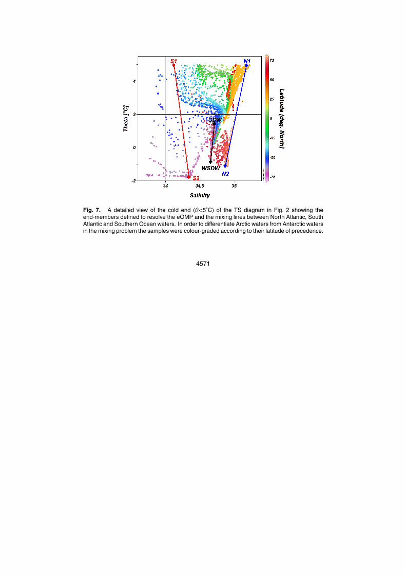
mixing through the length of the Eastern Atlantic basin. They have been named as N1,N2, S1, S2, Weddell Sea Deep Water (WSDW) and Circumpolar Deep Water (CDW)(Figs. 2 and 7).
The mixing of northern water masses in the Eastern Atlantic basin has been simpli-fied in this work by defining the N1 and N2 end-members (Figs. 2 and 7). Although10
none of them represents any known water source, they were characterized from theobserved upper limits of the salinity and temperature variability ranges. Rigorouslyspeaking, N1 is made up of about 13% of MW and 87% of LSW, which is one of themost important components of NADW. The N2 end-member has very similar thermo-haline characteristics to the Denmark Strait Overflow Water (DSOW) that forms in the15
Greenland Sea (Strass et al., 1993). The Iceland-Scotland Overflow Water (ISOW:1.9◦C, 34.98) (Alvarez et al., 2004) can also be found along the mixing line establishedbetween N1 and N2.
On the Southern Ocean end, the linear mixing of different proportions of the S1 andS2 end-members can yield several water masses that form in the upper South Atlantic,20
namely: Antarctic Intermediate Water (AAIW), Sub-Antarctic Mode Water (SAMW),Ice Shelf Water (ISW) and Winter Water (WW) (Brea et al., 2004; Lo Monaco et al.,2005). Moreover, some deep-waters like the CDW and the Weddell Sea Deep Water(WSDW) are also found on this end of the Atlantic (Figs. 2 and 7). The CDW formsfrom the mixing of WSDW with deep waters from the three major oceans in the Antarctic25
Circumpolar Currents (Broecker et al., 1985; Onken, 1995; Brea et al., 2004). On theother hand, WSDW is formed from the mixing of ISW and the overlying Warm DeepWater in the Weddell Sea (Onken, 1995). The thermohaline type values of CDW listedin Table 3 were taken from measurements made at the Drake Passage (Broecker et
4553
al., 1985). In the case of the type values for nitrate, phosphate and silicate for the sixend-members in Fig. 7, they were obtained by extrapolation of the ad hoc propertiesfrom regression lines with S and θ (Poole and Tomczak, 1999). Afterwards, thesepreliminary type values were run through an iterative process as in Alvarez et al. (2004)in order to refine the estimates.5
The A◦T and ∆Cdis type values in Table 3 were calculated by first identifying each
end-member within the subsurface layer and then applying Eqs. (1) and (2), respec-tively. In the case of CDW, the former procedure to calculate A◦
T and ∆Cdis cannot beapplied. Even though the θ and S type values of this end-member are enclosed withinthe observed thermohaline subsurface variability (Figs. 2, 3a and b), the fact that this10
water mass forms off-bounds the Atlantic basin from the mixing of WSDW with deepwaters from the three major oceans requires treating it separately. The θ-S type valuesfor CDW here used (Table 3) were obtained from measurements at the Drake Pas-sage (Broecker et al., 1985). To estimate the ∆Cdis and A◦
T type values, the CDW wasdecomposed into its constituent proportions of North Atlantic Deep Water (NADW),15
Antarctic Intermediate Water (AAIW) and WSDW, after Broecker et al. (1985). Accord-ing to Broecker et al. (1985) the CDW is formed by deep mixing of 25%, 45% and 30%of Northern component, Southern component and AAIW, respectively. The Southerncomponent in Broecker et al. (1985) corresponds with the WDSW end-member in thepresent work, while the so-called Northern component is made up of 60% of N1 and20
40% of the N2 end-members in this study. Finally, the AAIW in Broecker et al. (1985)would correspond to a mix of 93% of S1 and 7% of S2.
The obtained eOMP results show high correlation coefficients (R2, Table 3) and lowstandard errors of the residuals (Table 3) with the measured tracer concentrations. Thismeans that the simplified mixing model here presented is able to reproduce with a high25
degree of confidence the physical and chemical variability observed in the EasternAtlantic basin. In terms of reliability, the results here obtained are comparable to thosein other studies, such as in Karstensen and Tomczak (1998) or Alvarez et al. (2004),for example.
4554
Acknowledgements. We would like to extend our gratitude to the Chief Scientists, scientistsand the crew who participated and put their efforts in the oceanographic cruises utilized inthis study, particularly to those responsible for the carbon, CFC, and nutrient measurements.This study was developed and funded by the European Commission within the 6th FrameworkProgramme (EU FP6 CARBOOCEAN Integrated Project, Contract no. 511176), Ministerio de5
Educacion y Ciencia (CTM2006-27116-E/MAR), Xunta de Galicia (PGIDIT05PXIC40203PM),Accion Integrada Hispano-Francesa (HF2006-0094) and the French research project OVIDE.M. Vazquez-Rodrıguez is funded by Consejo Superior de Investigaciones Cientıficas (CSIC)I3P predoctoral grant program I3P-BPD2005. Funding for Richard G. J. Bellerby was providedfrom grant no. 511176 (GOCE).10
References
Alvarez, M., Perez, F. F., Shoosmith, D. R., and Bryden H. L.: The unaccounted role of Mediter-ranean Water in the draw-down of anthropogenic carbon, J. Geophys. Res., 110, 1–18,doi:10.1029/2004JC002633, 2005.
Alvarez, M., Perez, F. F., Bryden, H. L., and Rıos, A. F.: Physical and biogeochemical15
transports structure in the North Atlantic subpolar gyre, J. Geophys. Res., 109, C03027,doi:10.1029/2003JC002015, 2004.
Azetsu-Scott, K., Jones, E. P., Yashayaev, I., and Gershey, R. M.: Time series study of CFCconcentrations in the Labrador Sea during deep and shallow convection regimes (1991–2000), J. Geophys. Res., 108(C11), 3354, doi:10.1029/2002JC001317, 2003.20
Bates, N. R., Michaels, A. F., and Knap, A. H.: Seasonal and interannual variability of theoceanic carbon dioxide system at the U.S. JGOFS Bermuda Atlantic Time-series Site, Deep-Sea Res. Pt. II, 43(2–3), 347–383, 1996.
Bellerby, R. G. J., Olsen, A., Furevik, T., and Anderson L. A.: Response of the surface oceanCO2 system in the Nordic Seas and North Atlantic to climate change, in: Climate Variability25
in the Nordic Seas, edited by: Drange, H., Dokken, T. M., Furevik, T., Gerdes, R., and Berger,W., Geophysical Monograph Series, AGU, 189–198, 2005.
Berelson, W. M., Balch, W. M., Najjar, R., Feely, R. A., Sabine, C., and Lee, K.: Relating esti-mates of CaCO3 production, export, and dissolution in the water column to measurements of
4555
CaCO3 rain into sediment traps and dissolution on the sea floor: A revised global carbonatebudget, Global Biogeochem. Cy., 21, GB1024, doi:10.1029/2006GB002803, 2007.
Biastoch, A., Volker, C., and Boning, C. W.: Uptake and spreading of anthropogenic tracegases in an eddy-permitting model of the Atlantic Ocean, J. Geophys. Res., 112, C09017,doi:10.1029/2006JC003966, 2007.5
Brea S., Alvarez-Salgado, X. A., Alvarez, M., Perez, F. F., Memery, L., Mercier, H., and Messias,M. J.: Nutrient mineralization rates and ratios in the Eastern South Atlantic, J. Geophys. Res.,109, C05030, doi:10.1029/2003JC002051, 2004.
Brewer, P. G.: Direct observations of the oceanic CO2 increase. Geophys. Res. Lett., 5, 997–1000, 1978.10
Brewer, P., Wong, G., Bacon, M., and Spencer, D.: An oceanic calcium problem? Earth Planet.Sci. Lett., 26, 81–87, 1975.
Broecker, W. S.: “NO” a conservative water mass tracer, Earth Planet. Sc. Lett., 23, 8761–8776,1974.
Broecker, W. S. and Peng, T.-H.: Tracers in the Sea, Columbia University, Eldigio Press, New15
York, 690 pp., 1982.Broecker, W. S., Takahashi, T., and Peng, T.-H.: Reconstruction of past atmospheric CO2
contents from the chemistry of the contemporary ocean, Rep. DOE/OR-857, US Dept. ofEnergy, Washington, D. C., 79 pp., 1985.
Chen, C. T. and Millero, F. J.: Gradual increase of oceanic carbon dioxide, Nature, 277, 205–20
206, 1979.Clayton, T. D. and Byrne, R. H.: Calibration of m-cresol purple on the total hydrogen ion con-
centration scale and its application to CO2-system characteristics in seawater, Deep SeaRes. Pt. I, 40, 2115–2129, 1993.
Corbiere A., Metzl, N., Reverdin, G., Brunet, C., and Takahashi, T.: Interannual and decadal25
variability of the oceanic carbon sink in the North Atlantic subpolar gyre, Tellus, 1–11,doi:10.1111/j.1600-0889.2006.00232 2007.
Curry, R., Dickson, B., and Yashahaev, I.: A change in the freshwater balance of the AtlanticOcean over the past four decades, Nature, 426, 826–829, 2003.
Curry, R. and Mauritzen, C.: Dilution of the Northern North Atlantic in Recent Decades, Sci-30
ence, 308, 1772–1774, 2005.Dickson, A. G. and Millero, F. J.: A comparison of the equilibrium constants for the dissociation
of carbonic acid in seawater media, Deep-Sea Res., 34A(10), 1733–1743, 1987.
4556
DOE: Handbook of the Methods for the Analysis of the Various Parameters of the CarbonDioxide System in Sea Water, Version 2, ORNL/CDIAC-74, edited by: Dickson, A. G. andGoyet, C., 1994.
Doney, S. C. and Jenkins, W. J.: The effect of boundary conditions on tracer estimates ofthermocline ventilation rates, J. Mar. Res., 46, 947–965, 1988.5
Fine, R. A., Rhein, M., and Andrie, C.: Using a CFC effective age to estimate propagation andstorage of climate anomalies in the deep western North Atlantic Ocean, Geophys. Res. Lett.,29(24), 2227, doi:10.1029/2002GL015618, 2002.
Fraga, F. and Alvarez-Salgado, X. A.: On the variation of alkalinity during the photosynthesis ofphytoplankton, Cienc. Mar., 31, 627–639, 2005.10
Friis, K.: A review of marine anthropogenic CO2 definitions: introducing a thermodynamic ap-proach based on observations, Tellus, 58B, 2–15, doi:10.1111/j.1600-0889.2005.00173.x,2006.
Gruber, N.: Anthropogenic CO2 in the Atlantic Ocean, Global Biogeochem. Cy., 12, 165–191,1998.15
Gruber, N., Sarmiento, J. L., and Stocker, T. F.: An improved method for detecting anthro-pogenic CO2 in the oceans. Global Biogeochem. Cy., 10, 809–837, 1996.
Hall, T. M., Waugh, D. W., Haine, T. W. N., Robbins, P. E., and Khatiwala, S.: Estimates ofanthropogenic carbon in the Indian Ocean with allowance for mixing and time-varying air-sea CO2 disequilibrium, Global Biogeochem. Cy., 18, GB1031, doi:10.1029/2003GB002120,20
2004.Harvey, H. W.: The Chemistry and Fertility of Sea Waters, 2nd edn., Cambridge Univ. Press,
New Cork, 240 pp., 1969.Heinze, C.: Simulating oceanic CaCO3 export production in the greenhouse, Geophys. Res.
Honjo, S. and Manganini, S. J.: Annual biogenic particle fluxes to the interior of the NorthAtlantic Ocean; studied at 34◦ N 21◦ W, Deep-Sea Res., 40, 587–607, 1993.
IPCC: Summary for Policymakers, in: Climate Change 2007: Impacts, Adaptation and Vulner-ability. Contribution of Working Group II to the Fourth Assessment Report of the Intergov-ernmental Panel on Climate Change, Cambridge University Press, Cambridge, UK, 7-22,30
2007.Karstensen, J. and Tomczak, M.: Age determination of mixed water masses using CFC and
oxygen data, J. Geophys. Res. Oceans, 103(C9), 18599–18609, 1998.
4557
Kortzinger, A., Mintrop, L., and Duinker, J. C.: On the penetration of anthropogenic CO2 intothe North Atlantic ocean, J. Geophys. Res., 103, 18681–18689, 1998.
Lab Sea Group: The Labrador Sea Deep Convection Experiment, B. Am. Meteorol. Soc.,79(10), 2033–2058, 1998.
Lefevre, N., Watson, A. J., Olsen, A., Rıos, A. F., Perez, F. F., and Johannessen, T.: A decrease5
in the sink for atmospheric CO2 in the North Atlantic, Geophys. Res. Lett., 31, L07306,doi:10.1029/2003GL018957, 2004.
Lee, K., Choi, S.-D., Park, G.-H., Wanninkhof, R., Peng, T.-H., Key, R. M., Sabine, C. L., Feely,R. A., Bullister, J. L., Millero, F. J., and Kozyr, A.: An updated anthropogenic CO2 inventoryin the Atlantic Ocean, Global Biogeochem. Cy., 17(4), 1116, doi:10.1029/2003GB002067,10
2003.Levitus, S. et al.: Anthropogenic warming of the earth’s climate system, Science, 292, 267–270,
2001.Lo Monaco, C., Metzl, N., Poisson, A., Brunet, C., and Schauer, B.: Anthropogenic CO2 in
the SO: Distribution and inventory at the Indian-Atlantic boundary (World Ocean Circulation15
Experiment line I6), J. Geophys. Res, 110, C06010, doi:10.1029/2004JC002643, 2005.Luger, H., Wallace, D. W. R., Kortzinger, A., and Nojiri, Y.: The pCO2 variability in the midlati-
tude North Atlantic Ocean during a full annual cycle, Global Biogeochem. Cy., 18, GB3023,doi:10.1029/2003GB002200, 2004.
Martin, J. H., Fitzwater, S. E., Gordon, R. M., Hunter, C. N., and Tanner, S. J.: Iron, primary20
production and carbon-nitrogen flux studies during the JGOFS North Atlantic Bloom Experi-ment, Deep-Sea Res. Pt. II, 40, 641–653, 1993.
Matear, R. J., Wong, C. S., and Xie, L.: Can CFCs be used to determine anthropogenic CO2?Global Biogeochem. Cy., 17(1), 1013, doi:10.1029/2001GB001415, 2003.
Matsumoto, K. and Gruber, N.: How accurate is the estimation of anthropogenic carbon in25
the ocean? An evaluation of the ∆C∗ method, Global Biogeochem. Cy., 19, GB3014,doi:10.1029/2004GB002397, 2005.
Millero, F. J., Zhang, J. Z., Lee, K., and Campbell, D. M.: Titration alkalinity of seawater, Mar.Chem., 44, 153–156, 1993.
Millero, F. J., Lee, K., and Roche, M.: Distribution of alkalinity in the surface waters of the major30
oceans, Mar. Chem., 60, 95–110, 1998.Milliman, J. D., Troy, P. J., Bakch, W. M., Adams, A. K., Li, Y.-H., and Mackenzie, F. T.: Biolog-
ically mediated dissolution of calcium carbonate above the chemical lysocline? Deep-Sea
4558
Res. Pt. I, 46, 1653–1669, 1999.Mintrop, L., Perez, F. F., Gonzalez-Davila, M., Santana-Casiano, M. J., and Kortzinger, A.: Alka-
linity determination by potentiometry: Intercalibration using three different methods, Cienc.Mar., 26(1), 23–37, 2002.
Naegler, T., Ciais, P., Rodgers, K., and Levin, I.: Excess radiocarbon constraints on air-sea5
gas exchange and the uptake of CO2 by the oceans, Geophys. Res. Lett., 33, L11802,doi:10.1029/2005GL025408, 2006.
Olsen, A., Omar, A. M., and Bellerby, R. G. J., Magnitude and origin of the anthropogenic CO2increase and 13C Suess effect in the Nordic seas since 1981, Global Biogeochem. Cy., 20,GB3027, doi:10.1029/2005GB002669, 2006.10
Onken, R.: The spreading of Lower Circumpolar Deep Water into the Atlantic Ocean, J. Phys.Oceanogr., 25, 3051–3063, 1995.
Ono, T, Watanabe, S., Okuda, K., and Fukasawa, M.: Distribution of total carbonate and relatedproperties in the North Pacific along 30E N, J. Geophys. Res., 103, 30873–30883, 1998.
Orsi, A. H., Smethie Jr., W. M., and Bullister, J. L.: On the total input of Antarctic waters to the15
deep ocean: A preliminary estimate from chlorofluorocarbon measurements, J. Geophys.Res., 107(C8), 3122, doi:10.1029/2001JC000976, 2002.
Perez, F. F., Mourino, C., Fraga, F., and Rıos, A. F.: Displacement of water masses and reminer-alization rates off the Iberian Peninsula by nutrient anomalies. J. Mar. Res., 51(4), 869–892,1993.20
Perez, F. F. and Fraga, F.: A precise and rapid analytical procedure for alkalinity determination.Mar. Chem., 21, 169–182, 1987.
Perez, F. F., Alvarez, M., and Rıos, A. F.: Improvements on the back-calculation technique forestimating anthropogenic CO2, Deep-Sea Res. Pt. I, 49, 859–875, 2002.
Poole, R. and Tomczak, M.: Optimum multiparameter analysis of the water mass structure in25
the Atlantic Ocean thermocline, Deep Sea Res. Pt. I, 46, 1895–1921, 1999.Pond, S. and Pickard, G. L.: Introductory Dynamical Oceanography, 2nd edn, Pergamon Press,
Massachusetts, USA, 329 pp., 1983.Rhein, M. and Hinrichsen, H. H.: Modification of Mediterranean water in the Gulf of Cadiz, stud-
ied with hydrographic, nutrient and chlorofluoromethane data, Deep-Sea Res. Pt. I, 40(2),30
267–291, 1993.Riebesell, U., Zondervan, I., Rost, B., Tortell, P. D., Zeebe, R. E., and Morel, F. M. M.: Reduced
calcification of marine plankton in response to increased atmospheric CO2, Nature, 407,
4559
364–367, 2000.Rıos, A. F., Alvarez–Salgado, X. A., Perez, F. F., Bingler, L. S., Arıstegui, J., and Memery, L.:
Carbon dioxide along WOCE line A14: water masses characterization and anthropogenicentry, J. Geophys. Res., 108(C4), 3123, doi:10.1029/2000JC000366, 2003.
Rıos, A. F., Johnson, K. M., Alvarez-Salgado, X. A., Arlen, L., Billant, A., Bingler, L. S., Branel-5
lec, P., Castro, C. G., Chipman, D. W., Roson, G., and Wallace, D. W. R.: Carbon dioxide,hydrographic, and chemical data obtained during The R/V Maurice Ewing Cruise in the SouthAtlantic Ocean (WOCE Section A17, 4 January–21 March 1994), Carbon Dioxide Informa-tion Analysis Center, Oak Ridge National Laboratory, ORNL/CDIAC-148, NDP-084, 1–27,Oak Ridge, Tennessee, USA, 2005.10
Rıos, A. F., Anderson, T. R., and Perez, F. F.: The carbonic system distribution and fluxes in theNE Atlantic during Spring 1991, Prog. Oceanog., 35, 295–314, 1995.
Rosenheim, B. E., Swart, P. K., Thorrold, S. R., Eisenhauer, A., and Willenz, P.: Salinity changein the subtropical Atlantic: Secular increase and teleconnections to the North Atlantic Oscil-lation, Geophys. Res. Lett., 32, L02603, doi:10.1029/2004GL021499, 2005.15
Royal Society: Ocean acidification due to increasing atmospheric carbon dioxide, Document12/05, Royal Society, London, ISBN-0-85403-617-2, 68 pp., 2005.
Sabine C. L., Feely, R. A., Gruber, N., Key, R. M., Lee, K., Bullister, J. L., Wanninkhof, R.,Wong, C. S., Wallace, D. W. R., Tilbrook, B., Millero, F. J., Peng, T.-H., Kozyr, A., Ono, T.,and Rıos, A. F.: The oceanic sink for anthropogenic CO2, Science, 305, 367–371, 2004.20
Sabine, C. L. and Feely, R. A.: Comparison of recent Indian Ocean anthropogenic CO2 esti-mates with a historical approach, Global Biogeochem. Cy., 15(1), 31–42, 2001.
Sabine, C. L., Key, R. M., Johnson, K. M., Millero, F. J., Poisson, A., Sarmiento, J. L., Wal-lace, D. W. R., and Winn, C. D.: Anthropogenic CO2 inventory of the Indian Ocean, GlobalBiogeochem. Cy., 13, 179–198, 1999.25
Santana-Casiano, J. M., Gonzalez-Davila, M., and Laglera, L. M.: The carbon dioxide systemin the Strait of Gibraltar, Deep-Sea Res. Pt. II, 49, 4145–4161, 2002.
Sarma, V. V. S. S., Ono, T., and Saino, T.: Increase of total alkalinity due to shoaling of arago-nite saturation horizon in the Pacific and Indian Oceans: Influence of anthropogenic carboninputs, Geophys. Res. Lett., 29(20), 1971, doi:10.1029/2002GL015135, 2002.30
Siegenthaler, U. and Sarmiento, J.: Atmospheric carbon dioxide and the ocean, Nature, 365,119–125, 1993.
Strass, V. H., Fahrbach, E., Schauer, U., and Sellmann, L.: Formation of Denmark Strait Over-
4560
flow Water by mixing in the East Greenland Current, J. Geophys. Res., 98, 6907–6919,1993.
Takahashi, T., Sutherland, S. C., Sweeney, C., Poisson, A., Metzl, N., Tilbrook, B., Bates, N.,Wanninkhofe, R., Feely, R. A., Sabine, C., Olafsson, J., and Nojiri, Y., Global sea-air CO2flux based on climatological surface ocean pCO2, and seasonal biological and temperature5
effects, Deep Sea Res. Pt. II, 49, 1601–1622, 2002.Thomas, H. and Ittekkot, V.: Determination of anthropogenic CO2 in the North Atlantic Ocean
using water mass ages and CO2 equilibrium chemistry, J. Mar. Sys., 27, 325–336, 2001.Touratier, F., Azouzi, L., and Goyet, C.: CFC-11, ∆14C and 3H tracers as a means to assess
anthropogenic CO2 concentrations in the ocean, Tellus, 59B, 318–325, doi:10.1111/j.1600-10
0889.2006.00247.x, 2007.Vazquez-Rodrıguez, M., Touratier, F., Lo Monaco, C., Waugh, D. W., Padin, X. A., Bellerby,
R. G. J., Goyet, C., Metzl, N., Rıos, A. F., and Perez, F. F.: Anthropogenic carbon distributionsin the Atlantic Ocean: data-based estimates from the Arctic to the Antarctic, Biogeosciences,6, 439–451, 2009,15
http://www.biogeosciences.net/6/439/2009/.Wallace, D. W. R.: Storage and transport of Excess CO2 in the Oceans: The JGOFS/WOCE
Global CO2 Survey: Ocean Circulation and Climate, edited by: Siedler, G., Church, J., andGould, J., 489–521, Academic Press, San Diego – California, 2001.
Wanninkhof, R., Peng, T. H., Huss, B., Sabine, C. L., and Lee, K.: Comparison of inorganic20
carbon system parameters measured in the Atlantic Ocean from 1990 to 1998 and recom-mended adjustments, ORNL/CDIAC-140, Oak Ridge Natl. Lab., US Dept. of Energy, OakRidge, Tenn, 43 pp., 2003.
Wanninkhof, R., Doney, S. C., Peng, T. H., Bullister, J. L., Lee, K., and Feely, R. A.: Comparisonof methods to determine the anthropogenic CO2 invasion into the Atlantic Ocean. Tellus, 51B,25
511–530, 1999.Waugh, D. W., Hall, T. M., McNeil, B. I., Key, R., and Matear, R. J.: Anthropogenic
CO2 in the oceans estimated using transit time distributions, Tellus B, 58B, 376–389,doi:10.1111/j.1600-0889.2006.00222.x, 2006.
4561
Table 1. List of selected Atlantic cruises (Fig. 1). Only data collected at depths greater than100 m was used for calculations. Surface layer data was discarded to avoid the influence ofseasonal variability on Cant estimates.
Parameters Analyzed AdjustmentsSection Date P.I. CT AT fCO2 pH Freons N P Si O CT AT
A02 6 Nov–7 Mar 1997 P. Koltermann Ya Y Nb N Y Y Y Y Y NAc NAAR01 23 Jan–24 Feb 1998 K. Lee Y Y Y Y Y Y Y Y Y NA NAA14 1 Nov–2 Nov 1995 H. Mercier Y Y+Calcd N N Y Y Y Y Y NA NAA16 4 Jul–29 Aug 1993 R. Wanninkhof Y Y Y Y Y Y Y Y Y NA NAA16N 4 Jun–11 Aug 2003 J. Bullister Y Y Y Y Y Y Y Y Y NA NAA17 1 Apr–21 Mar 1994 L. Memery Y Y+Calc N Y Y Y Y Y Y NA −8e
A20 17 Jul–10 Aug 1997 R. Pickart Y Y Y N Y Y Y Y Y NA NAA25 (OVIDE) 6 Jun–5 Jul 2002 H. Mercier N Y Y Y Y Y Y Y Y NA NAI06-Sa 23 Jan–9 Mar 1993 A. Poisson Y Y Y N Y Y Y Y Y NA NAI06-Sb 20 Feb–22 Mar 1996 A. Poisson Y Y Y N Y Y Y Y Y NA NANSeas 1 Jun–7 Jun 2002 R. Bellerby Y Y N N Y Y Y Y Y NA NA
Acronyms and superscripts denote the following:a Y=measured values available;b N=measured values unavailable;c NA=no adjustment made;d Y+Calc=When direct measurements were unavailable, AT was calculated from CT and pHmeasurements, using the thermodynamic relationships of the carbon system;e =Correction in µmol kg−1, after ORNL/CDIAC 148 report
4562
Table 2. Coefficients and statistics for the Multilinear Regression (MLR) of ∆Cdis vs. conser-vative parameters (Eq. 3). Except for θ (◦C) and S, all other variables and standard errorsare given in µmol kg−1. N stands for the number of valid points used for the fit, and R2 is thecorrelation coefficient of the adjustment. The standard error of the estimate was calculated asσ/
√N.
Region Latitude Band θ Interval [◦C] a b (θ−10) c (S-35) d (NO-300) e (PO-300) N R2 Std. error
Table 3. The equations, weights and type values of the selected end-members for the eOMP.The correlation coefficient (R2) between eOMP results and observed properties and the stan-dard errors of these estimates are also listed. All type values and standard errors are given inµmol kg−1 except for θ (◦C) and S. Notice that neither the A◦
T nor the ∆Cdis equations (dark greyshade) belong to the system of equations for the eOMP (no weight assigned). The type valueshere listed were calculated a posteriori and are given as reference for the end-members herechosen.
Fig. 1. Map showing Atlantic cruises used to characterise the subsurface layer. The cruisesdenoted by stars were also selected for testing the adequacy of proposed modifications in Cantestimation (Sect. 4).
4565
Cant determination from Atlantic sub-surface observations
19
it. These are the NSeas-Knorr, CLIVAR A16N, WOCE I06-Sb and WOCE A14
transects (Fig. 1).
Figure 4. T/S diagram of the Atlantic from the studied data set. Red circles represent South Atlantic sub-surface waters; blue circles are North Atlantic sub-surface waters. The smaller dark dots represent all water column (depth >200 dbar) T/S samples. The smaller light grey dots are the uppermost 25 meters surface waters showing a clear distinction from the rest of the tighter bulk of samples. The thick yellow diamonds joined by the red line are the end-members that define the mixing triangle used to resolve the influence of MW. The thick orange triangles joined by the green line are the end-members used in the OMP mixing analysis applied to waters with θ<5º C (refer to section 4.3.2 for details).
Since there exist overlapping latitudes between the A16N-A14 and A14-I06Sb
section pairs a few stations have been discarded. The general selection criteria followed
was choosing the stations that were deepest and had the least influence of Indian Ocean
waters. Accordingly, the northernmost ends of the A14 and I06Sb cruises are omitted
from the analysis. The observed thermohaline variability in the Eastern Atlantic section
is presented in Figure 4. As in Figure 3, surface (uppermost 25 m) and sub-surface (100-
200 m) waters have been highlighted over the rest of the water column data. It is
Salinity
θ [ºC
]
Fig. 2. TS diagram of the Atlantic from the studied dataset (Fig. 1 and Table 1). Red circlesrepresent South Atlantic subsurface (100–200 m) waters and blue circles are North Atlanticsubsurface waters. The smaller dark dots represent samples collected deeper than 200 m.The small light-grey dots are the uppermost 25 m surface waters, showing a clear distinctionfrom the rest of the tightly-wrapped bulk of samples. The thick yellow diamonds joined withthe red line are the end-members that define the mixing triangle used to resolve the influenceof Mediterranean Water (Sect. 3). The thick orange triangles joined by the green line are theend-members used in the extended Optimum Multiparameter (eOMP) mixing analysis used tocalculate A◦
T and ∆Cdis in waters below the 5◦C isotherm (Sect. 3).
4566
Cant determination from Atlantic sub-surface observations
21
Figure 5. Sub-surface layer (100-200 m) distributions of several properties from the selected Eastern Atlantic cruises: a) Potential temperature; b) Salinity; c) Silicate; d) Ages from CFC-12 data; e) NPAT; f) ΔCdis.
ΔCdis
Fig. 3. Subsurface layer (100–200 m) distributions of several properties from the selected At-lantic cruises (Fig. 1): (a) Potential temperature (θ, in ◦C); (b) Salinity; (c) Silicate (µmol kg−1);(d) Age estimates from CFC12 data (years); (e) NPAT (µmol kg−1); (f) ∆Cdis (µmol kg−1) calcu-lated from the original definition in Gruber et al. (1996) (see Eq. 2).
4567
Cant determination from Atlantic sub-surface observations
27
[Broecker and Peng, 1982]. Additionally, data from sediment traps in the North Atlantic
corroborates the dissolution of CaCO3 in the upper layers of this ocean [Honjo and
Manganini, 1993; Martin et al., 1993]. The ATº parameterization from this study
produces positive ΔCa values in the whole Atlantic and low ΔCa in the Nordic Seas.
Both ΔCa distributions agree on the accumulation of calcium and increasing alkalinity
in deep waters, mainly in the Deep South Atlantic where the oldest water masses are
found.
Figure 6. Distributions of computed CaCO3 dissolution (µmol·kg-1) using: a) the ATº parameterization from L’03; and b) the ATº parameterization given in equation (1) from this study.
Fig. 4. Distributions of computed CaCO3 dissolution (∆Ca, in µmol kg−1) using: (a) the A◦T pa-
rameterization from Lee et al. (2003). The light-purple blur indicates negative ∆Ca estimates(CaCO3 precipitation). Only the isopleth of −5 µmol kg−1 was added in this region as a refer-ence, but values of ∆Ca as low as −17 µmol kg−1 are reached; (b) the A◦
T parameterization inEq. (1) from this study.
4568
Cant determination from Atlantic sub-surface observations
51
Figure 9. Cant distributions (µmol·kg-1) of the Atlantic Ocean calculated with: a) The ϕCTº method, which includes results for the NSeas cruise; b) The ∆C* method from GSS’96 as of L’03 for cruises CLIVAR A16N, WOCE A14 and I06-Sb. Negative values are omitted and shown as blank areas. The thick white line in 9a and 9b is the 5 ºC isotherm. The contribution of the “ϕ” term to individual Cant estimates is shown in c) (µmol·kg-1) by subtracting Cant calculated (equation 10) using ϕ=0 and ϕ=0.55. Data from all cruises has been referenced to 1994.
Fig. 5. Cant distributions (µmol kg−1) of the Eastern Atlantic basin calculated with: (a) The ϕC◦T
method and (b) The ∆C∗ method as of Lee et al. (2003) for latitudes below 60◦ N, where theirA◦
T parameterization is valid. Negative Cant estimates are omitted and shown as blank areas.The thick white isoline in (a) and (b) is the 5◦C isotherm to indicate the regions where A◦
T and∆Cdis are calculated with different procedures, according to the ϕC◦
T method. The effect ofthe “ϕ” term in individual Cant estimates is shown in (c) (in µmol kg−1). This was calculated bysubtracting Cant calculated from Eq. (10) with ϕ=0 and then ϕ=0.55. The results have beenreferenced to 1994.
4569
Cant determination from Atlantic sub-surface observations
56
them in Fig. 10. If the ΔΔCdis term discussed and parameterized in this study is to be
omitted, an average increase on the specific inventory of 6.8 ±2.8 mol·C m-2 occurs
(12% of the average Cant inventory). This is in good agreement with the average 7%
reduction factor proposed in MG’05. The long term variation of ATº produces an
increase on the average specific inventory of 8.3 ±2.0 mol C·m-2. It must also be noticed
that the influences of the ΔΔCdis term and the long-term variation of ATº in Cant
inventories vary little with latitude, as represented in Figure 10. The ∆C* method does
not consider the long-term variability of ΔCdis nor ATº.
Figure 10. Comparison of specific Cant inventories (mol C·m-2) for the Eastern Atlantic calculated using: The ∆C* method from GSS’96 (green line); The ∆C* method as of L’03 (blue line); The ϕCTº method (red line). All three inventories have been averaged by latitude bands and referenced to 1994, after L’03. Orange line with open circles depicts the combined effects of CaCO3 and temperature shifts introduced in PATº. The grey line with open squares represents the individual contribution of the φ term to the ϕCTº specific inventory when φ=0.
Effect of the temporal variability of ATº Effect of the “ϕ” term
(ϕ=0)
Fig. 6. Comparison of specific inventories of Cant (mol C m−2) of the Eastern Atlantic calculatedusing the ∆C∗ method as in Gruber et al. (1996) (green line), the ∆C∗ method as in Lee etal. (2003) (blue line) and the ϕC◦
T method (red line). All inventory results were averaged bylatitude bands and referenced to 1994, after Lee et al. (2003). The orange line with open circlesgives the magnitude of the combined effects on the inventories of CaCO3 and increasing SST,introduced through the PA◦
T parameterization given in Eq. (1). The grey line with open squaresrepresents the individual contribution to the ϕC◦
T specific inventory of the ϕ term (i.e., whenϕ=0).
4570
Cant determination from Atlantic sub-surface observations
36
simplified defining the N1 and N2 end-members in the TS diagram from Figure 7. The
N1 end-member does not represent any known water source. It was defined from the
observed upper limits of the salinity and temperature variability ranges. Rigorously
speaking, N1 is made up of about 13% of MW and 87% of LSW, which is one of the
most important components of the NADW. As a matter of fact, the N1 end-member is
very close to the upper limb of the NADW (uNADW) as in Brea et al. (2004).
Alternatively, the N2 end-member has a very similar thermohaline imprint to the
Greenland Sea Deep Water (GSDW) and other several main contributors of the Arctic
overflows [Olsson et al., 2005]. It can be closely compared to the lower limb of the
NADW (lNADW) in Brea et al. (2004).
Figure 7. A detailed view of the cold (θ <5 ºC) end from the TS diagram in Fig. 4 that is used to spot the end-members defined to resolve the eOMP. The samples are color coded according to their latitude of precedence to differentiate Arctic and Antarctic waters in the mixing problem.
Fig. 7. A detailed view of the cold end (θ<5◦C) of the TS diagram in Fig. 2 showing theend-members defined to resolve the eOMP and the mixing lines between North Atlantic, SouthAtlantic and Southern Ocean waters. In order to differentiate Arctic waters from Antarctic watersin the mixing problem the samples were colour-graded according to their latitude of precedence.