Finance and Economics Discussion Series Divisions of Research & Statistics and Monetary Affairs Federal Reserve Board, Washington, D.C. Incentives and Prices for Motor Vehicles: What has been happening in recent years? Carol Corrado, Wendy Dunn, and Maria Otoo 2006-09 NOTE: Staff working papers in the Finance and Economics Discussion Series (FEDS) are preliminary materials circulated to stimulate discussion and critical comment. The analysis and conclusions set forth are those of the authors and do not indicate concurrence by other members of the research staff or the Board of Governors. References in publications to the Finance and Economics Discussion Series (other than acknowledgement) should be cleared with the author(s) to protect the tentative character of these papers.
Transcript
Finance and Economics Discussion Series Divisions of Research & Statistics and Monetary Affairs
Federal Reserve Board, Washington, D.C.
Incentives and Prices for Motor Vehicles: What has been happening in recent years?
Carol Corrado, Wendy Dunn, and Maria Otoo 2006-09
NOTE: Staff working papers in the Finance and Economics Discussion Series (FEDS) are preliminary materials circulated to stimulate discussion and critical comment. The analysis and conclusions set forth are those of the authors and do not indicate concurrence by other members of the research staff or the Board of Governors. References in publications to the Finance and Economics Discussion Series (other than acknowledgement) should be cleared with the author(s) to protect the tentative character of these papers.
Incentives and Prices for Motor Vehicles: What has been happening in recent years?
Carol Corrado, Wendy Dunn, and Maria Otoo* Federal Reserve Board
Washington, D.C.
June 2003 (Revised, January 2006)
* We thank Marie Degregorio and Matthew Wilson for their assistance; Robert Schnorbus and Matthew Racho at J.D. Power and Associates for helping us with the data; and Mark Bils, Darrel Cohen, Erwin Diewert, Charles Gilbert, Kathleen Johnson, and Jeremy Rudd for helpful discussions. The views expressed in this paper are those of the authors and should not be attributed to the Board of Governors of the Federal Reserve System or other members of its staff. This paper was prepared for the SSHRC International Conference on Index Number Theory and Price Measurement, Fairmont Waterfront Hotel, Vancouver, Canada, June 30-July 3, 2004. A preliminary version was given at the CRIW workshop on price measurement at the NBER Summer Institute, Cambridge, Mass., in June 2003.
Incentives and Prices for Motor Vehicles: What has been happening in recent years?
Carol Corrado, Wendy Dunn, and Maria Otoo January 2006
ABSTRACT
We address the construction of price indexes for consumer vehicles using data collected from a national sample of dealerships. The dataset contains highly disaggregate data on actual sales prices and quantities, along with information on customer cash rebates, financing terms, and much more. Using these data, we are able to capture the actual cash and financing incentives taken by consumers, and we demonstrate that their inclusion in measures of consumer vehicle prices is important. We also document other features of retail vehicle markets that interact and overlap with price measurement issues. In particular, we construct vehicle price indexes under different assumptions about what constitutes a Anew@ product in moving from one model year to the next. For the period that we study (1999 to 2003), a period during which incentives became more widespread and new model introductions rose, our preferred price index drops faster than the CPI for new vehicles.
KEYWORDS: Price indexes, motor vehicles, motor-vehicle financing.
Carol Corrado Wendy Dunn Maria Otoo
Stop 82 Division of Research and Statistics Federal Reserve Board Washington, D.C. 20551
1. Introduction Although motor vehicle manufacturers have used incentives to boost consumer sales for
some time, direct manufacturer-to-consumer incentives have become both more generous and
more widespread in recent years. Using data collected from a large national sample of motor
vehicle dealerships, we measure the value of two popular types of vehicle price incentives—cash
rebates and reduced-rate financing—and analyze their combined effect on the monthly prices of
consumer light vehicles.
Chart 1 shows our estimates of the average values of sales-weighted interest subvention
and cash rebates; the data and methods used to develop these estimates are discussed in the next
section. Cash rebates are a direct reduction in the retail vehicle price, and the chart plots the
value of the rebates used in each period relative to the number of vehicles sold in the period.
Reduced-rate financing programs lower the interest rate on financed vehicle purchases, and the
chart shows the present discounted value of the reduced payment stream resulting from these
programs in each period, again, relative to all vehicles sold in the period. In this paper, we refer
to the present discounted value of promotional interest rate reductions as interest rate subvention
or, simply, interest subvention.
The two types of incentives have grown in recent years. After varying little, on balance,
throughout 2000 and most of 2001, interest subvention shot up in October 2001. In the wake of
the attacks of September 11, General Motors announced a program that offered purchasers either
zero percent financing for up to sixty months or a cash rebate. This program proved to be
immensely popular. In response, most other motor vehicle manufacturers also offered zero
percent financing or sweetened their cash rebate programs. Chart 2 illustrates how widely used
these incentives have become. By the end of 2003, cash rebates are estimated to have been used
in about 57 percent of sales, and interest subvention is estimated to have occurred in a little more
than 40 percent of purchases. Most incentive programs allow the consumer to take either the
rebate or the special interest rate incentive but not both, and the specific vehicles with programs
vary throughout a year.
We believe these developments present challenges for how consumer prices are defined
and measured. In its measure of new vehicle prices for the consumer price index (CPI), the
Bureau of Labor Statistics (BLS) includes only information on cash rebates, even though the two
types of incentives need not be of equal value and both influence the price the consumer actually
2
pays for a vehicle. In addition, manufacturers often use the two types interchangeably, and the
empirical literature on consumer auto demand has shown that specific models of vehicles are
very price elastic (Houthakker and Taylor 1970; Berry, Levinson, and Pakes 1995). Thus, the
variation in the type and size of incentives offered with individual models may complicate the
construction of a monthly vehicle price index based on a fixed-weighted sample, or subset, of all
available models.
In this paper, we work with highly detailed monthly data on prices, quantities and
financing terms that allow us to study the workings of retail vehicle markets and to construct
vehicle price measures that fully account for interest subvention as well as customer cash
rebates. The data we use are based on a sample of dealerships, and, for each dealership, data on
sales of all models (and all trim levels of each model) are included. Our results suggest that price
measures that include both of these direct manufacturer-to-consumer incentives are necessary for
understanding developments in retail vehicle markets in recent years. For example, we calculate
monthly matched-model price indexes by model year. These indexes display an interesting
pattern in which vehicle prices drop noticeably over the model-year life cycle, in large part
because of the marketing incentives paid for by the manufacturers. In another finding, we
document an increase in the trend rate of manufacturers’ introductions of new and modified
vehicles, especially as the size and prevalence of incentives expanded. We also show that newly
produced vehicles from different model years are marketed simultaneously for an extended
period; that is, the model-year selling period is longer than a calendar year.
The overlap in the model-year selling periods in our data, as well as the generally
competitive nature of vehicle markets, suggests that matched-model techniques (Aizcorbe,
Corrado, and Doms 2000, 2003) can be used to construct vehicle price indexes that aggregate
over model years. Nonetheless, just as the increase in the size and variability of incentive
programs presents challenges for the measurement of consumer vehicle prices, so does the
increased rate at which makers have been introducing new and modified vehicles.
After introducing and reviewing our data, we establish the findings mentioned earlier and
then address the construction of incentive-adjusted price indexes for consumer vehicles that
aggregate over model years. Our work is grounded in conventional index number theory and
explores the effect on monthly price measures of using different assumptions about what is a
new product (or how to “match” prices of vehicles) as one model year ends and the next begins.
3
On the one hand, all models could be treated as new with the advent of a new model year; in this
case, the recurring model-year price drops are chained together and their cumulative effect over
successive years shows through in the aggregate price index. On the other hand, the price pattern
could be viewed as a seasonal phenomenon; in this case, the prices are “linked” so that the
recurring price drops are offset by recurring increases and little or none of the cumulative effect
shows through. Mark Bils (2004) has recently advocated the former approach; results of
Pashigian, Bowen, and Gould (1995) suggest that the BLS methods for compiling vehicle prices
for the CPI can be regarded, at least in part, as following the latter approach.1
Our conclusions are somewhat in the spirit of the findings by Bils (2004), but they are not
of the same quantitative size. Using our preferred price concept and matching method, we find
that consumer light vehicle prices fell 3-1/4 percent per year, on average, from the end of 1998 to
the end of 2003, nearly 2-1/2 percentage points per year faster than the decrease in the CPI for
new vehicles. Vehicle prices before adjusting for incentives edge down only 3/4 percent per year,
on average; nearly 2 percentage points of the average decline in our preferred incentive-adjusted
price index is due to the inclusion of cash rebates, and 3/4 percentage point is attributable to
interest subvention.
2. Data and Concepts
The data we use in our analysis are from a database called Power Information Network
(PIN) Explorer, which is generated by J.D. Power and Associates (JDPA). The database contains
information on motor vehicle transactions that is collected from dealerships around the country
and uploaded daily from the dealerships’ finance and insurance (F&I) systems. JDPA reviews
and checks the data for reporting or clerical errors before making them available to subscribers in
PIN Explorer. According to the company, the PIN sample represents 70 percent of the
geographical markets in the United States.2 Within those markets, JDPA collects data from
1 Pashigian, Bowen, and Gould (1995) showed that the behavior of the not seasonally adjusted car price data in the CPI accords well with what theory would predict for the behavior of prices of a “fashion” good. Price drops for fashion goods over a selling period are regarded as seasonal phenomena. Not all of the price drops for vehicles in the CPI sample are treated as seasonal phenomena; indeed, a portion is treated in what Bils (2004) regards as the appropriate way. 2 PIN collects data in a number of U.S. markets and in Canada. The U.S. geographic markets as of late 2003 were Boston, New York, Philadelphia, Pittsburgh, Baltimore/Washington DC, Charlotte, Atlanta, Orlando, Tampa, Miami, Houston, Dallas/Fort Worth, Tulsa/Oklahoma City, St. Louis, Indianapolis, Cleveland, Memphis/Nashville, Chicago, Detroit, Minneapolis/St. Paul, Denver, Phoenix, Los Angeles/San Diego, San Francisco/Sacramento, and Seattle/Tacoma/Portland.
4
roughly one-third of the dealerships and, all told, captures about 20 percent of national retail
transactions.3
PIN Explorer is incredibly rich and includes detailed information on the price, cost, and
type of vehicles sold or in inventory in each period, as well as data on F&I activity, including the
value and terms of the loans received by customers who financed their vehicle purchase through
the dealerships. A few demographic variables, such as customer age, are also collected. To
examine vehicle prices and incentives, this study uses just a few key price and financing
variables in the PIN Explorer database (table 1). Note that the information we use is for both
purchased and leased vehicles; the PIN variables for leased transactions are generated in such a
way as to make them comparable to series on purchased vehicles.4
Our observations are monthly averages of the PIN national level data for new motor
vehicles by model and model year from late 1998 through 2003. An example of our primary unit
of observation would be the monthly sales (in units) of the 2001 Mercury Sable and the average
price (unit value) of the 2001 Mercury Sables sold in a particular month. We do not have access
to the data on the individual purchases from which the information in PIN Explorer is
constructed, but our model-level-by-model-year database contains about 35,000 monthly
observations and consists of essentially the full PIN sample for the period we study.
We refer to the price measures we develop and use in this study as “actual transaction”
prices or, simply, “actual” prices. By “actual” price we mean the price that individual consumers
actually paid, on average, to purchase a given vehicle in a given month. To generate the actual
transaction price, we start with the PIN vehicle price at the level of our unit of observation
(model by model year). We then subtract (1) the PIN data on customer cash rebates and (2) our
estimate of the value of interest subvention. In the next four sections, we discuss more fully the
definition of the PIN vehicle price, the methods used to estimate interest subvention, and the
homogeneity of PIN’s model-by-model-year unit of observation, and we present summary
averages of the data.
3 By manufacturer, the coverage ranges from roughly 15 percent to 25 percent. 4 For example, for leased transactions, PIN calculates an internal rate of return based on the discounted future cash flows associated with the purchase; cash flows for leases include the residual value, monthly payments, and fees such as points, application costs, and security deposits. This calculation results in a rate that is comparable to the interest rate paid on (financed) purchased vehicles (the annual percentage rate, or APR, as defined in the Federal Reserve Board’s Regulation Z).
5
The PIN vehicle price. The PIN vehicle price incorporates most of the major ways in
which retailers influence the price the consumer actually pays for a vehicle. First, it reflects the
effect of haggling between the dealer and the consumer. The price the dealer and consumer agree
to in a purchase or lease contract is recorded in PIN, and dealer concessions, such as upgrades in
accessories or trims provided at no (or below) cost, are captured because the average price for a
particular model-by-model-year vehicle in our database is directly affected by the prevalence (or
relative absence) of such concessions. Second, the PIN vehicle price reflects the amount a
customer receives for a vehicle trade-in. Detailed information on trade-in vehicles is available in
PIN, and when a buyer receives a price for a trade-in that is greater or less than its market value,
this difference—called an overallowance or underallowance—is recorded and used to adjust the
contract price.5 Third, PIN records the amount of the “cash-back” that the customer receives
from the manufacturer. The cash rebate is a separate field in the F&I reporting system and the
variable is systematically recorded with each transaction in the underlying PIN data.
All told, the PIN vehicle price less the cash rebate is the dollar price, adjusted by the
trade-in allowance, that the customer pays for the vehicle and for factory- and dealer-installed
accessories and options contracted for at the time of the sale. The PIN vehicle price excludes
sales taxes as well as charges for service contracts, financing insurance, and other F&I products
sold by the dealership. Although PIN Explorer has information on the prices customers pay for
these products and services, we exclude such products and services from our pricing analysis
because they are generally purchased after the transaction price is negotiated.6 At times,
manufacturers offer buyers free service contracts at no additional cost, but the value of these
giveaways is excluded from our price measure.7
In constructing the CPI for new motor vehicles, the BLS attempts to capture the actual
transaction price, but the resulting BLS measure differs from our PIN-based measure in several
important ways. First, the CPI includes sales taxes but excludes an adjustment for the value of
vehicle trade-ins. Second, the CPI incorporates an estimated value for service contracts that are
5 As noted in JPDA’s Pin Explorer Glossary, when a trade-in is involved in a transaction, the actual price of the vehicle can be masked from the customer. Two identically-equipped vehicles can be sold at the same underlying price to two customers, yet the prices printed on the customers’ contracts can appear very different. 6 For further details on the measures in the PIN database, see PIN Explorer Glossary, J. D. Power and Associates (2003). 7 A limitation of the data is that PIN Explorer records no information on service contracts that are given away. When a service contract is purchased at a reduced price, however, the value of the contract will appear in PIN along with other related information.
6
provided at no cost to the consumer but refrains from measuring or recording the value of
interest subvention. Third, the CPI is compiled from monthly sample data at the individual
transaction level but is not designed to reflect the actual acceptance rate of each incentive
program. When consumers are given a choice of either cash back or reduced-rate financing, the
BLS subtracts the average value of cash rebates during the preceding thirty days from the sticker
price regardless of the incentive program the consumer actually selected.8 We estimate that in
2003, the vast majority (more than 70 percent) of manufacturers’ incentive promotions allowed
consumers to take reduced-rate financing in lieu of, or in addition to, a cash rebate offer.9 The
remaining programs included only reduced-rate financing.
All told, the BLS methodology probably captures the majority (but certainly not all) of
the incentive programs in some fashion. However, the incidence of cash rebates and interest
subvention varies notably over time, and the average values of the two types of incentives are
usually unequal. Although the PIN data we use are not at the individual transactions level, our
PIN-based prices will reflect the actual monthly variation in the size and incidence of incentives
shown in charts 1 and 2. We thus believe that the PIN vehicle price less the cash rebate is a
highly accurate measure. Indeed, the adjustment for trade-in allowances and the availability of
related statistics on leasing and financing suggests that the PIN data have certain advantages over
the CPI’s sample data for studying and measuring consumer vehicle prices.
Interest subvention. Interest subvention occurs when a consumer receives an interest rate
for a vehicle purchase through a manufacturer’s financial services company (GMAC, Ford
Financial, Honda Financial Services, and so on) that is lower than the interest rate that could
have been obtained elsewhere. Although interest subvention is a direct manufacturer-to-
consumer incentive that affects the price the consumer actually pays for a vehicle, unlike
customer cash rebates, interest subvention cannot be observed directly and must be estimated.
To estimate interest subvention, we use the PIN interest rate received by customers who
financed or leased new vehicles through dealerships and compute the present value of the
difference between the monthly payment stream under this rate and the stream under an 8 To estimate the CPI for new motor vehicles, the BLS begins with the vehicle’s sticker price. It then adjusts the sticker price to arrive at a transactions price. According to the BLS Handbook of Methods (page 29), “When pricing new vehicles, BLS economic assistants obtain separately all the components of the sticker price. This includes the base price and the price for options, dealer preparation, transportation, etc.” Since 1998, the CPI has excluded the line item, “automobile finance charges,” which was separate from the index for new vehicles. 9 The calculation is based on incentive programs offered by the six largest-selling manufacturers in the United States: General Motors, Ford, Chrysler, Toyota, Honda, and Nissan.
7
alternative rate the buyer would pay at an outside, independent lending source. The difference
between the two payment streams is discounted to the present at a constant rate of 4 percent. The
alternative rate is determined from information published in the Federal Reserve’s Survey of
Consumer Finances (SCF) and from the new car loan rate published in the Federal Reserve’s
To compute the actual payment stream, we need information on the loan amount, loan
length, and interest rate that consumers actually receive. As indicated in table 1, PIN provides
these measures. Unfortunately, the PIN measures that we have are for all customers who finance
(or lease) their vehicle through dealerships, whereas ideally we would like to have measures that
exclude the transactions in which the lender (or lessor) is not owned by the manufacturer.10
However, we believe that this distinction is of little practical importance because the overall
percentage of dealer-financed transactions in which the lender is not owned by the manufacturer
is relatively small. The data from PIN for 2002 and 2003 show that, on average, less than
15 percent of dealer-financed sales used independent lenders in those years.11
To compute the alternative monthly payment stream, we need a measure for the
alternative rate that the buyer would pay at an outside, independent lending source. The
alternative rate that we start with is the forty-eight-month commercial motor vehicle loan rate
issued by the Federal Reserve Board. This rate is obtained from a survey of commercial banks in
which respondents are asked to report their “most common” interest rate for new forty-eight-
month motor vehicle loans; the published aggregate is the average of these reported rates. A
benefit of using this rate is its ready availability. However, a downside is that using it assumes
that all consumers face the same alternative interest rate regardless of creditworthiness.
The creditworthiness of a potential buyer depends on a variety of factors. However, age
(the primary buyer characteristic that we have available) is useful in assessing the interest rate
that a buyer is likely to receive. Data from the 2001 SCF indicate that, as a respondent’s age
10 For ease of exposition, we will omit references to lease transactions in the discussion that follows. Of course, the subvention estimates we develop fully capture the effects of lease promotions (“no down payment”, “no lease-end fees”, and so on) if such promotions actually lower the lessor’s implied rate of return on a lease transaction. 11 Nonetheless, if independent financing through dealerships is a significant source of interest subvention, our measure will overstate the manufacturer-to-consumer concept that we want. We believe this possibility to be highly unlikely, however. When a customer fills out a loan application at a dealership, often the dealership submits the application to a number of lenders. If an independent lender accepts the customer’s loan application, a wholesale rate is quoted to the dealership. The dealership may then quote a higher rate to the customer, and this rate becomes the observed retail rate (if the transaction is consummated). The spread between wholesale and retail rates has traditionally been an important source of dealership revenue.
8
increases, the average interest rate on new vehicle loans drops steadily (table 2). In our data,
customer age varies substantially across models, and this variation removes any illusion of buyer
homogeneity.
Next, we report the results of regressions that use a variety of series to explain the interest
rate that SCF respondents received for new vehicle loans (table 3). All of the loans in the
estimation originated in the years 1999 through 2001. As shown in column 1 of the table, the
coefficient on the average age of the respondent is negative and statistically significant.
Regressions in columns 2 and 3 include income and wages, respectively, as well as other
variables. In addition to age, home ownership and educational attainment are important
explanatory variables for the new vehicle loan rate that SCF respondents received. When these
additional variables are included, the coefficient on age decreases in size but remains statistically
significant.12
We used the coefficient estimate in column 1 to adjust the alternative interest rate in our
calculations by the average customer age for each model in each month. For models with an
average customer age equal to the mean of the whole sample, the alternative interest rate is the
forty-eight-month commercial bank rate. For models with a customer age lower than the overall
sales-weighted mean (44-1/2 years), the alternative rate was increased 0.05 percentage point for
each year below the mean. Thus, a model with a mean customer age of 18 years would have an
alternative interest rate roughly 1-1/4 percentage points higher than would a model with a mean
customer age of 44-1/2 years. Models with average customer ages greater than the overall
average would have lower rates.
Another assumption in using the forty-eight-month bank rate as an alternative rate is that
it serves as a reasonable proxy for rates that buyers could have received from other lenders. In
PIN, loans financed through outside lenders are recorded as “cash” transactions, and no
information is collected on the terms of these loans. We again turned to the SCF to obtain
additional information. Table 3 also shows regression results that control for lending source. We
use dummy variables for loans obtained from captive finance companies, credit unions, and
finance companies. The results, shown in column 4, are reported relative to an alternative in
which loans are obtained from commercial banks. As seen in the coefficient estimates, rates on
12 Note that the coefficients on income and wages are insignificant when home ownership and educational attainment are included in the regressions.
9
loans from captive finance companies and credit unions were each more than 1 percentage point
less than those on loans at commercial banks. In contrast, loans from finance companies carried
interest rates that were about 1-1/2 percentage point higher than those from commercial banks.13
The results in column 4 suggest that the commercial bank rate that we use in our analysis
may overstate the alternative rate for customers who otherwise would have used a credit union.
On the other hand, it may understate the alternative rate for customers of finance companies.
Nevertheless, given the limited demographic data available in PIN Explorer, we believe that the
aggregate forty-eight-month commercial bank rate that uses customer age to adjust for
creditworthiness is a reasonable proxy for the alternative lending rate that is needed to estimate
interest subvention.
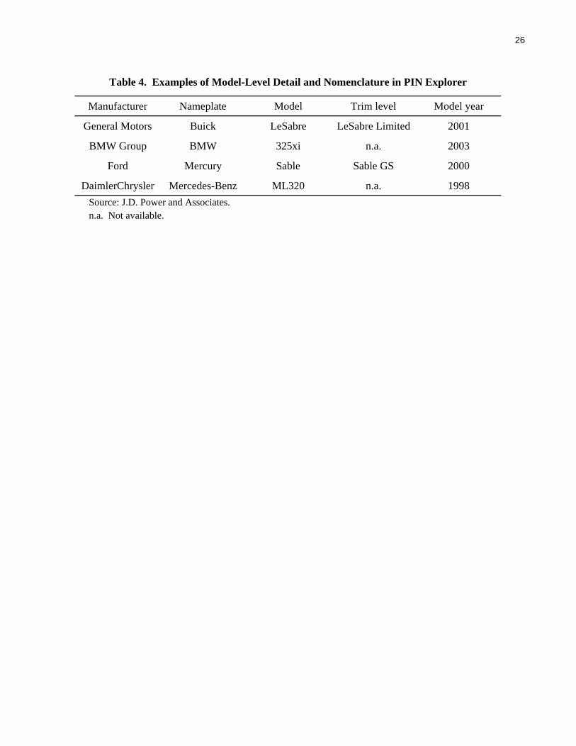
Unit of observation. As indicated earlier, our primary unit of observation is by model and
model year, but for many vehicles our PIN model-level observations are more detailed than is
suggested by the term “model.” Moreover, PIN Explorer contains what it calls “trim level”
observations that are even more detailed than its model-level observations that we use. Table 4
provides examples of our model-level detail as well as our nomenclature. For example, in our
sample, we include the model Buick LeSabre. The trim-level appellation is Buick LeSabre
Limited. However, for some models in our sample (for example, the Mercedes ML320 or the
BMW 325xi), no further level of detail is available. Thus, PIN covers these models (or “series”
of cars) at essentially the trim level.
We next compare the model-level observations available in the data issued by Ward’s
Communications, a leading source of information on the motor vehicle industry, with the model-
level observations available in PIN. We use the model year 2002 for illustration. In the Ward’s
data, 16 models accounted for the top one-third of all light vehicle sales. The middle one-third
was accounted for by another 42 models and the bottom one-third by more than 200 others. By
contrast, 34 PIN models accounted for the top one-third of sales, a number more than twice as
large as the corresponding Ward’s number, and PIN’s model count for the second one-third was
also much larger with a count of 65. Besides PIN’s distinctions for “series” of cars, such as the
BMW and Mercedes vehicles noted earlier, much of the additional stratification available in PIN
13 The coefficient estimates in column 4 changed little when the home ownership and educational attainment variables were added to the regression.
10
models relative to Ward’s models occurs in “lines” of popular light trucks and sport-utility
vehicles, or SUVs (Ford F-150, Ford F-250, Silverado 1500, Silverado 2500, and so on).
PIN’s trim-level observations are much more granular than their model-level data. In our
work to construct vehicle price indexes from PIN model-level data, we exploit information from
these highly detailed data. We do not work directly with the trim-level observations because the
transactions count for many of the trims in the bottom third of sales is extremely thin. In
addition, the information on trim levels that we have (in terms of the types of variables) is
limited before January 2001.14
Summary averages of the data. We calculate the aggregate average values of our
incentive and price measures for each year from 1999 to 2003 and for the period as a whole; the
data are sales-weighted (table 5). We estimate that direct manufacturer-to-consumer incentives
on new vehicle purchases averaged nearly $1,500 from 1999 to 2003 and that interest subvention
and cash rebates were about equal in value, on average. The average value of cash rebates
skyrocketed over the period, however, and the average value of incentives in 2003 was nearly
triple that in 1999.
The average actual price that consumers paid for a vehicle was about $24,000 and rose
noticeably between 1999 and 2003. By 2003, the overall average selling price (ASP) was
$25,000, and the ASP for trucks was more than $4,000 larger than that for cars. From 1999 to
2003 (on a December to December basis, not shown in the table), the overall ASP rose
2-1/2 percent per year. Excluding incentives, the ASP of vehicles rose 3-1/2 percent per year.
With regard to financing during the 1999 to 2003 period, the average interest rate
received for new vehicle loans peaked in 2000 at 8.2 percent but fell subsequently to an average
of 5.4 percent in 2003. Over the same period, the average loan term for dealer-financed loans
rose from about four years to nearly five years. Low interest rates and longer terms allowed
consumers to keep monthly payments low even as the average amount financed rose. From 1999
to 2003, the average amount financed climbed almost 13 percent, while the average actual price
paid for a new vehicle increased 6-3/4 percent.15
14 The second limitation refers to the data from PIN Explorer that are available to us; this is not an inherent limitation of the information collected by JPDA for inclusion in PIN. 15 This differential does not necessarily reflect an increase in the loan-to-value ratio. Consumers may chose to finance sales taxes and the F&I products (service contracts, insurance) or additional items (fabric protector, paint sealants) purchased from the dealership, and the prices (or quantities) of these items may have increased more than the vehicle price during this period.
11
3. Retail Vehicle Markets in Recent Years
In addition to incentives becoming more generous and widespread, other developments in
retail vehicle markets in recent years interact and overlap with the measurement of consumer
vehicle purchase prices.
New model introductions. We report the number of PIN models by model year for the
model years 1998 to 2004 (table 6). All told, our database has observations on more than
500 unique PIN models, and, on average, about 260 of the models were sold in adjacent model
years.16 We also show the number of PIN models that were newly introduced in each year as
well as statistics that we derived on continuing models for which major redesigns were made or
for which new trim levels became available (without major redesigns). We define a major
redesign as a platform change and a new trim level as a name change in PIN’s trim-level
observations.17 In 2001, the number of new models in PIN Explorer jumped to nearly 60 and has
since remained elevated. The count of redesigns showed no trend during the period we study, but
the number of new trims also jumped in 2001 and has remained at what looks to be a relatively
high rate.
The rise in new model introductions that began with the 2001 model year is confirmed by
both Ward’s model-year statistics (see last column of table 6) and Ward’s monthly sales data on
the number of unique models sold, shown in chart 3 to display a longer perspective. As
illustrated in the chart, the number of models sold changed little from 1995 to 1999, but rose
dramatically beginning in 2000 with the introduction of 2001 model year vehicles. Many of the
newly introduced models were new varieties of SUVs, which are profitable and popular types of
light trucks. The new trim levels were also disproportionately concentrated among SUVs and
consisted of upgrades in interior finishing and electronics (such as navigation systems), larger
engines, or other driving and safety features.
16 The database that we construct from the raw PIN data uses 490 PIN models rather than the 506 PIN models available to us because of the need to drop 16 models with missing or problematic observations. The dropped models account for an extremely small, negligible portion of total sales. 17 A platform is the basic structure of a vehicle; we used Ward’s data on vehicle platforms by model year to identify models that had been through major redesigns. For PIN models more disaggregate than Ward’s models, we used information from Internet sources (new vehicle reviews and summary articles on vehicle redesigns) to make the identification. We also used Internet sources to verify the accuracy of trim change counts for models with two or more name changes.
12
Our data are thus capturing an important development in vehicle markets in recent
years—namely, that manufacturers noticeably expanded the number of models and trims that
they produced and marketed. We believe PIN Explorer is especially well suited to pick up the
price implications of this development. Because the PIN data are collected from a sample of
dealerships, information on sales of new and modified model sales are recorded in the system at
the time of introduction. But price collectors (who select and track specific vehicles to obtain
price information) or compilers of model-level list prices (who must pick a particular trim level
for each model) may be challenged by having to choose representative vehicles during a period
of rapid change.
Sales over the model year. We report information on the number of continuing, entering,
and exiting models, by quarter within each model year (table 7). These figures highlight several
key within-model-year properties of vehicle markets. First, as indicated by the row labeled
“Total continuing” models, a significant portion of the total number of marketed models in any
given period is available for computing a price change. Second, as seen in the rows that break
out continuing models, by model year, the new vehicles available for sale in each period are from
more than one model-year vintage; indeed, in many instances, vehicles from three different
vintages are available for sale in the same quarter. Third, as shown in the row labeled “Entering,”
most new vehicle vintages are introduced in the third quarter, a reflection of the well-known
model-year changeover pattern in production. By contrast, the clearing of older vehicles from
dealers’ lots, shown in the row labeled “Exiting,” occurs relatively smoothly over the calendar
year.
All told, the quarterly data in the table illustrate that newly produced vehicles of a given
model year are almost always marketed simultaneously with newly produced vehicles of an
adjacent model year. Chart 4 shows this pattern in more detail by plotting monthly expenditure
shares by model year over time. As can be seen in the chart, the sales cycle for each model-year
vintage typically runs for about eighteen months (from July through December of the following
year) and, consequently, it overlaps with the sales cycle of vehicles in preceding and subsequent
model years for a considerable time. Shifts in purchases of new model-year vehicles occur most
often during the late summer and early fall (August, September, and October). Unlike the abrupt
13
model-year changeover in production, the transition in spending from one model year to the next
occurs relatively more smoothly.18
The relatively smooth pattern of initial sales of new model-year vehicles in the late
summer and early fall differs from the pattern that existed many years ago. We lack high-
frequency data on sales by model year for earlier periods to confirm the exact timing and nature
of the shift, but we can observe the evolution of the seasonal factor for aggregate monthly sales
from the late 1970s to the present.19 Seasonal factors for recent years lead us to expect above-
average sales in July and August and average or slightly below-average sales in September and
October. Factors for the late 1970s for these months expected sales to be substantially above-
average in October and below-average otherwise. By segment, the results for domestic autos are
the most striking. The October seasonal factor for domestic auto sales was 112 in 1977 but
gradually fell over the years and was 91 in 2003.
4. Price Indexes for Consumer Vehicles
The availability of price and quantity information for a nontrivial number of essentially
identical products whose prices are available in adjacent monthly periods suggests that matched-
model techniques can be used to construct price indexes for consumer vehicles. A long,
distinguished literature has addressed the use of a hedonic approach to measure quality-adjusted
prices for motor vehicles (Griliches 1961, Triplett 1969, Gordon 1990, among others), but these
studies had to rely almost exclusively on annual data on list prices at the start of each model
year. By contrast, we are able to work with data that conform to the demands of conventional
index number theory—very detailed, comprehensive monthly data on actual prices and
quantities.
The matched-model Törnqvist price index, which is grounded in conventional index
number theory, is a weighted geometric mean of price ratios of homogeneous items, denoted by
the subscript “j” that uses an average of each item’s revenue share in the two periods as weights.
In logs, the aggregate price change from t-1 to t is expressed as follows:
18 These different production and spending patterns by model year show through in the composition and age of dealers’ inventory by model year. The automaker’s inventory control problem and its implications for manufacturers’ pricing decisions are explored in Copeland, Dunn, and Hall (2005). 19 We wish to thank our colleague Dan Vine for pointing us in this direction.
14
(1)
/ 1
/ 1 / 1
1 , , , 1 M
, , , . 1 . 1 M M
1 / 2
where
1,....T
ln ln (ln ln ),
/ /
t t
t t t t
t t j t j t j tj
j t j t j t j t j tj j
t
P P s P P
s PQ PQ PQ PQ
−
− −
− −∈
− −∈ ∈
=
− = −
⎡ ⎤= +⎣ ⎦
∑
∑ ∑
Summation over matched models is denoted as / 1 M
,t tj −∈∑ where Mt is the set of unique goods
produced or sold in each period and Mt/t-1, (that is, Mt ∩ Mt-1) is the set of goods produced or sold
in adjacent periods.
When the results of (1), as well as those of the closely related Fisher formula, are chained
together over T periods, the price index is exact for periods before and after changes in the
composition of Mt/t-1 (Diewert 1987). Although this procedure makes no special allowance for
entry and exit, if entering and exiting items are essentially perfect substitutes for continuing
items (and if we make certain assumptions about consumer preferences), the resulting aggregate
price index approximates an exact index for all periods, not just those in which there are no
compositional changes in Mt/t-1 (Feenstra 1994). Accordingly, we use (1) both to observe the
pattern of prices by model year and to construct an aggregate price index across all vehicles in
the sample.
Price indexes by model year. We assume that the mix of sales among trims exhibits no
trend over a model year and that the PIN models (our unit of observation) are essentially
homogeneous across monthly observations. Under these conditions, our model-level price data
(unit values) are the appropriate data for measuring aggregate price change (Balk 1998), and we
can compute (1) from the monthly PIN model-level data for each model year (see table 7).
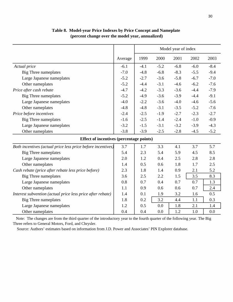
In table 8, we summarize the model-year price declines by reporting annualized five-
quarter changes (from the third quarter of the introductory year to the fourth quarter of the
following year) for various price measures and for subcategories grouped by nameplate. The
results illustrate clearly that significant and broad-based declines in vehicle prices occurred over
all model years in the sample. As noted earlier, a potential explanation for these recurring price
declines is that more fashion-oriented, or price-inelastic, shoppers purchase vehicles early in the
model year, while more price sensitive consumers wait until later in the model year. If this were
the case, we would expect to see a similar declining pattern in the average buyer age, our best
15
proxy for income. However, we found that the aggregate average buyer age did not vary
systematically over the model year.
By comparing the different price measures, one can see that the magnitude of the drop in
vehicle prices over the model year increases as the price concept is broadened to capture all
forms of incentives. Our measure of the actual price, which nets out both cash rebates and
interest subvention, decreases, on average, at an annual rate of 6.1 percent over the model life
cycle. By contrast, the model-year price declines before incentives average just 2.4 percent over
the same period. The within-year patterns of these indexes are displayed in chart 5, in which one
can see that the drop in the actual price is often steeper at the beginning and at the end of the
model year cycle. The indexes also show that the within-year price declines accelerated over the
sample period and that the difference between prices before and after incentives widened as well.
Looking at the effects of incentives for the various nameplate categories, one can see that
the Big Three (General Motors, Ford, and Chrysler) consistently use cash rebates to reduce
prices. These rebates increased at an average annual rate of 3.6 percent over the model year, and
in model year 2003 they jumped more than 8 percent. At the large Japanese firms (Toyota,
Honda, and Nissan), cash rebates are not nearly as popular as they are at the Big Three. Only in
the most recent model year in the sample did these firms begin to use cash rebates more
intensively.
Beginning in the 2000 model year, financing incentives also became more prevalent,
particularly for the Big Three nameplates. When General Motors offered zero-interest finance
rates on most of its models after the terrorist attacks on September 11, 2001, the value of interest
subvention increased sharply, contributing 3.2 percentage points to the decline in actual prices
over the model year. Although the increase in interest subvention in 2001 was most pronounced
for the Big Three nameplates, a pickup in these incentives for the large Japanese nameplates was
also noticeable. Expenditure patterns shifted dramatically over this period, as a large share of
consumers substituted away from cash rebates and accepted the financing incentives (see
chart 2). This pattern is especially apparent in the divergence between the broadest price measure
and the measure that just excludes cash rebates. These two price measures differ most noticeably
from 2001 to 2003.
Next, we report changes in the model-year price indexes for cars versus trucks and for
eight vehicle market segments using our preferred price concept (table 9). One can see that, for
16
the most part, prices for the various vehicle segments tend to decline at about the same rate over
the model year once both cash rebates and interest subvention are taken into account. One
notable exception, however, is full-size cars, which appear to have much steeper price declines
over the model year than do other vehicle segments. The difference mainly reflects more
generous incentives for the segment, as prices before incentives fall at about the same rate for
full-size cars as for cars in other vehicle segments. With price declines averaging just
5.6 percent, the indexes for luxury cars exhibit the smallest price reductions over the model year,
and incentives for this segment contribute just 0.6 percentage points to the overall decrease.
Finally, we report changes in the model-year actual prices disaggregated by models that
were new or major redesigns versus models that continued from the previous year with no major
change (table 10). In a given model year, the grouping of “new” models makes up between
15 percent and 25 percent of the total number of unique models sold (see the second and fourth
columns of table 5 relative to the first column of the table). Differences in price movements
between these two categories will have implications for aggregate price indexes over time
because, as will be described shortly, they represent one view of which models are new goods
and which are continuing goods. Nevertheless, as can be seen in the table, although the value of
incentives increases more for models that are not new or redesigned, the overall price declines by
model year are fairly similar for both categories.
Aggregate consumer vehicle prices. The richness of our data suggests that an aggregate
price index—not just price indexes by model year—can also be computed using (1). The
resulting measures, however, depend critically on the interpretation of what defines a unique
good. In particular, the results depend on which vehicles can and cannot be considered similar
across model years or, put differently, they rely on how the observations in our dataset should be
“matched” in (1) when moving from one model year to the next.
To illustrate this problem, we consider three alternatives for “matching”: First, we
assume that vehicles of different model years have virtually identical features until they undergo
a major redesign. In this situation, we match adjacent observations for a given model,
irrespective of model year, except in cases in which the vehicle has been through a major
redesign. Once redesigned, these model-year vehicles are treated as separate goods in (1), along
with the vehicles that newly enter the market in a given model year. Second, we treat both
redesigned vehicles and vehicles with new trim options as new goods; otherwise, the price index
17
is compiled according to the same procedure as used in the first alternative. As noted earlier,
manufacturers greatly expanded the trim options they offered on existing models during the
sample period. In the case of the second alternative, therefore, the number of vehicles treated as
entering goods in (1) is more than double the number under the first alternative. Finally, we treat
all models at the close of one season versus those at the beginning of another as separate goods
in (1). This third alternative is consistent with the view that, with every new model year, the
physical characteristics of a vehicle change sufficiently so that we can only match adjacent-
month prices for a given model in a given model year, in which case the number of new goods in
(1) is equal to the number of vehicles in each model year.
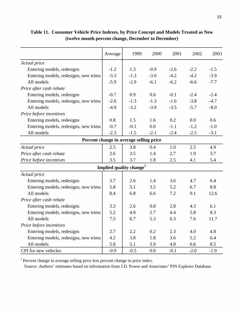
We calculate the aggregate indexes that result from the three matching assumptions and
for the various price measures (table 11). Regarding the results for the actual price, the index that
treats all models as unique goods drops most sharply over time: The twelve-month changes drop
6 percent, on average, over the five-year period. This large cumulative drop essentially reflects
the chaining together over time of the recurring within-year model-year price declines shown
earlier.20 Moreover, under this matching assumption, the price declines appear to have
accelerated in recent years, registering an estimated decline of nearly 8 percent over 2003. By
contrast, the matching assumption that treats only entering models and redesigned models as
separate goods results in a price index that falls just slightly more than 1 percent per year, on
average, and the declines do not appear to have accelerated in recent years.
The matching assumption that treats both redesigned models and model-year vehicles
with trim changes as new products results in an average aggregate price decline that falls in
between the rates implied by the two other indexes—actual consumer vehicle prices drop
3-1/4 percent per year, on average, when we use this intermediate assumption. Because there are
many examples of models and trims that, from one model year to the next, are virtually
identical—except for their model-year designations—one could argue that the intermediate
assumption yields the most appropriate price index. Certainly, in view of the results presented in
table 6, we would have difficultly arguing that only new and redesigned models (the first
alternative) are all that are “new” as one model year ends and the next begins.
20 Indeed, indexes calculated under the third matching assumption are equivalent to indexes calculated using model-year expenditure shares (previously shown in chart 4) to aggregate the model-year matched-model price indexes (previously shown in chart 5) according to equation (1).
18
One could also argue, however, that because of the interaction between new and used
vehicle markets, and because the model year is an easily observable product characteristic that is
strongly correlated with the age of a vehicle, the treatment of all model-year vehicles as separate
goods (the third alternative) may best reflect the underlying consumer preferences that drive
prices downward over the model year. However, we believe this line of reasoning suggests that
recurring price declines are seasonal (related to obsolescence, the loss of “newness”) rather than
reflecting persistent declines in the actual price of new vehicles.21
A logical implication of the view that recurring price declines are seasonal is to formally
treat vehicles as “weakly seasonal” commodities and to use one of the indexes suggested by
Diewert (1998, 1999; see also Balk 1980) for these types of goods. Applied to vehicles, these
indexes would match the price of a given model year vehicle in a month with the year-earlier
price of its year-earlier vintage. We investigated this approach and found that prices dropped less
than under our three primary alternatives, but were nonetheless very close to those calculated
using the first alternative. Note that seasonal index numbers exclude information on the prices
and market shares of entering (and redesigned) models until one year after their introduction (or
change). We believe the very high rate of new model introductions over the period we study
presents problems for using the seasonal index number approach to measure vehicle prices.
Notably, under all three of our primary matching assumptions, the index for the actual
vehicle price falls more rapidly than would be implied by the CPI for new vehicles (shown at the
bottom of the table). Arguably, the CPI concept falls somewhere between our actual price and
the PIN price after cash rebate (discussed earlier), and the CPI “matching” method is probably
closest to our first alternative (Pashigian, Bowen, and Gould 1995; Bils 2004). This suggests that
the differences between our preferred approach (the second matching alternative applied to the
actual price) and the CPI approach stem largely from differences in methods. Indeed, the CPI
measure of price change is between the results for the first matching method applied to the actual
price and those for this same method applied to the PIN price after cash rebate.
Implications for quality change. Our new estimates of vehicle price change have
implications for the associated measures of quality improvement and productivity that took place
in recent years. In the bottom half of table 11, we report the implied measures of quality change
21 Obsolescence is defined as the decline in the price of a newly produced asset (or a price index for a cohort of assets) in the presence of a new vintage of the asset, a definition and terminology drawn from the literature on economic depreciation. See Diewert (2005) for a recent review of this literature.
19
for each of the alternative matching assumptions and price measures. These rates are derived by
subtracting the constant-quality price change from the total change in vehicle price, as measured
by the change in the average selling price, or ASP.22 Although the size and variation in the
resulting estimates of quality change are substantial, when we base our calculation on the actual
price and the second matching assumption (our preferred measure), we find that the average
annual pace of quality improvement from 1999 to 2003 was nearly 6 percent per year.
Our estimates of quality change can be compared with those that Bils (2004) constructed
from micro CPI data. In that paper, the author argues that, contrary to current BLS methods used
for constructing price indexes for most goods, forced product substitutions should be treated the
same way that scheduled substitutions are treated--with price changes across substituted models
viewed as quality upgrades.23 This suggestion is closest to following our matching assumption
that treats every model-year vehicle as a new product. For motor vehicles, Bils finds that prices
for matched models declined an average of 3.3 percent per year from 1988 to 2003, a result that
when combined with the 4.0 percent increase in unit prices over the same period, implies that
quality advanced 7.3 percent per year. This figure is much faster than the 2.9 percent rate implied
by the current BLS methodology for motor vehicle price indexes.
As noted earlier, using our data on actual prices, we find that the matched-model index
that treats every model-year vehicle as a new product declined by nearly 6 percent per year, on
average, from 1999 to 2003. Coupled with the 2-1/2 percent increase in average selling prices,
this result implies that measured quality increased nearly 8-1/2 percent per year, a figure very
close to Bils’s estimate for the longer sample period. If the measure of price less cash rebate
measure is used, then our estimate of quality change is nearly identical to that derived by Bils.
5. Conclusion
In this paper we use a rich data set of monthly sales, transaction prices, and financing
terms to document several empirical observations on prices for motor vehicles. First, we show
that financing incentives play an integral role in understanding recent movements in aggregate
22 These changes, which are shown in the middle panel of the table, were calculated from the data on ASPs in dollars (shown on table 5). 23 At regular sample rotations, the BLS draws a new sample of stores and products within a geographic area to better reflect current consumer spending. Bils (2004) refers to these as scheduled substitutions. Forced substitutions occur when a store stops selling a particular product that is being priced, and the BLS agent substitutes another model of that brand or of a similar product.
20
vehicle prices. We also find that multiple vintages of the same models are often sold
simultaneously in retail vehicle markets, a practice that presents challenges as well as
opportunities for measuring vehicle purchase prices. We examine within-model-year price
movements and find that vehicle prices drop rapidly in the months after their introduction, often
in large part through the use of direct manufacturer-to-consumer incentives. Finally, we consider
the construction of a price index that uses matched-model techniques to aggregate over model
years.
The results of using a conventional index number approach to measure vehicle prices
depend crucially on which vehicles can and cannot be considered similar across model years.
Our preferred approach, which regards major redesigns and new trims as new (or separate)
goods, yields a price index for consumer vehicles that drops faster than the decline shown by the
CPI for the same period. We attribute this result to two developments—both relatively recent—
that we believe are incorporated more accurately in the price measure constructed using our data
and our approach. First, the rate at which manufacturers introduced new and modified models
increased dramatically beginning in 2000, and the CPI may have been slow to adapt to the
change, in effect treating many of the popular, expanded trim options as price increases. Second,
the value and incidence of interest subvention increased noticeably in late 2001 and in 2002 and
likely is not fully reflected in the CPI. All told, we find that the pace of quality improvement in
consumer vehicles averaged 6 percent per year from 1999 to 2003, a pace twice that implied by
official estimates.
21
References
Aizcorbe, Ana, Carol Corrado, and Mark Doms (2000). “Constructing Price and Quantity
Indexes for High Technology Goods,” paper presented at the CRIW workshop, National Bureau of Economic Research Summer Institute 2000, Cambridge, Mass., www.nber.org/~confer/2000/si2000/doms.pdf.
Aizcorbe, Ana, Carol Corrado, and Mark Doms (2003). “When Do Matched-Model and Hedonic
Techniques Yield Similar Measures?” Working Paper Series 2003-13. San Francisco: Federal Reserve Bank of San Francisco (June).
Balk, B.M. (1980). “A Method for Constructing Price Indices for Seasonal Commodities,”
Journal of the Royal Statistical Society, Series A (General), vol. 143 (1), pp. 68-75. Balk, B.M. (1998). “On the Use of Unit Value Indices as Consumer Price Subindices,” in
Walter Lane, ed., Proceedings of the Fourth Meeting of the International Working Group on Price Indices. Washington: U.S. Department of Labor, Bureau of Labor Statistics,
pp. 112-20. Berry, Steven, James Levinsohn, and Ariel Pakes (1995). “Automobile Prices in Market
Equilibrium,” Econometrica, vol. 63 (July), pp. 841-90. Bils, Mark (2004). “Measuring Growth from Better and Better Goods,” NBER Working Paper
Series 10606. Cambridge, Mass.: National Bureau of Economic Research, July. Bureau of Labor Statistics (1997). BLS Handbook of Methods. Washington: U.S. Department of
Labor, Bureau of Labor Statistics.
Copeland, Adam, Wendy Dunn, and George Hall (2005). “Prices, Production, and Inventories over the Automotive Model Year,” Finance and Economics Discussion Series 2005-25. Washington: Board of Governors of the Federal Reserve System, May.
Diewert, W. Erwin (1987). “Index Numbers,” in John Eatwell, Murray Milgate, and Peter
Newman, eds., The New Palgrave: A Dictionary of Economics, vol. 2. New York: Stockton Press, pp. 767-80.
Diewert, W. Erwin (1998). “High Inflation, Seasonal Commodities and Annual Index
Numbers,” Macroeconomic Dynamics, vol. 2 (December), pp. 456-71. Diewert, W. Erwin (1999). “Index Number Approaches to Seasonal Adjustment,”
Macroeconomic Dynamics, vol. 3 (March), pp. 48-68.
22
Diewert, W. Erwin (2005). “Issues in the Measurement of Capital Services, Depreciation, Asset Price Changes, and Interest Rates,” in Carol Corrado, John Haltiwanger, and Daniel Sichel, eds., Measuring Capital in the New Economy. Chicago: University of Chicago Press.
Feenstra, Robert C. (1994). “New Product Varieties and the Measurement of International
Prices,” American Economic Review, vol. 84 (March), pp. 157-77.
Gordon, Robert J. (1990). The Measurement of Durable Goods Prices. Chicago: University of Chicago Press.
Griliches, Z. (1961). “Hedonic Price Index for Automobiles: An Econometric Analysis of
Quality Change,” in The Price Statistics of the Federal Government, General Series 73. New York: National Bureau of Economic Research, pp. 137-96. Reprinted in
Z. Griliches (1971), ed., Price Indexes and Quality Change. Cambridge, Mass.: Harvard University Press.
Houthakker, Hendrik S., and Lester D. Taylor (1970). Consumer Demand in the United States:
Analyses and Projections. Cambridge, Mass.: Harvard University Press. J.D. Power and Associates (2003). PIN Explorer Glossary, mimeo, Power Information Network. Pashigian, Peter B., Brian Bowen, and Eric Gould (1995). “Fashion, Styling, and the Within-
Season Decline in Automobile Prices,” Journal of Law and Economics, vol. 38 (October), pp. 281-309.
Triplett, Jack E. (1969). “Automobiles and Hedonic Quality Measurement,” Journal of Political
Economy, vol. 77 (May-June), pp. 408-17.
23
Variable DefinitionVehicle price The price that a customer pays for a vehicle and for factory and dealer-
installed accessories and options, adjusted for the trade-in allowance. (The trade-in allowance is the difference, if any, between the amounts a dealer allows a customer for a trade-in and the wholesale market-value of the trade-in.) The vehicle price excludes the price of aftermarket options, fees, taxes, or service contracts.
Vehicle price less customer cash rebate
The price after manufacturer-to-consumer rebates. The customer cash rebate, the cash amount given to the customer, is subtracted from vehicle price.
Interest rate (APR/IRR rate)
The annualized percentage rate (APR) paid by a customer on a financed or leased vehicle. For finance transactions, the APR is as defined in the Federal Reserve Board’s Regulation Z. For leased transactions, PIN calculates an internal rate of return (IRR) that is comparable to the APR.
Term The number of months that a customer will make finance or lease payments on a vehicle.
Amount financed The portion of the total purchase price (including the cost of finance and insurance products) that is funded by a lender or lessor. Applies only to finance and lease transactions.
Customer age The age of the customer at the time of purchase or lease. Note: Includes purchased and leased vehicles. Source: PIN Explorer Glossary , J.D. Power and Associates (2003).
Table 1. Definition of Selected Variables in PIN Explorer
24
Mean 21-29 30-39 40-49 50-59 60-69 70 and over
Interest rate (percent) 11.2 10.2 9.4 9.1 8.9 7.2
Total household income1 48 108 142 603 494 71
Household wage income1 45 97 81 101 72 21 Note: In thousands of current dollars; reflects income in 2000; number of observations is 686. Source: Survey of Consumer Finances , 2001, Board of Governors of the Federal Reserve System.
Table 2. Interest Rates on New Vehicle Loans and the Average Age and Income of Buyers
Age of respondent (years)
25
Dependent variable: interest rate on new vehicle loans (1) (2) (3) (4)
Age -0.05 -0.02 -0.02 -0.05(0.01) (0.01) (0.01) (0.01)
Annual household income -0.08(0.50)
Annual wages and salaries -0.11(0.38)
Home ownership -2.32 -2.32(0.16) (0.16)
Educational attainment -1.15 -1.18(0.18) (0.18)
Lending source: Captive finance companies -1.28
(0.52) Credit unions -1.09
(0.45) Finance companies 1.53
(0.41) Note: Observations total 685. The data are unweighted. Each regression also included a variable to control for cyclical movements in interest rates. Regressions in columns 2 and 3 contained additional variables: number in household, race of respondent, gender of respondent, and type of vehicle purchased (automobile or light truck). The numbers in parentheses are standard errors.
1999-2001Table 3. Factors Affecting Interest Rates on New Vehicle Loans, Selected Results,
Source: Survey of Consumer Finances , 2001, Board of Governors of the Federal Reserve System.
26
Manufacturer Nameplate Model Trim level Model year
General Motors Buick LeSabre LeSabre Limited 2001
BMW Group BMW 325xi n.a. 2003
Ford Mercury Sable Sable GS 2000
DaimlerChrysler Mercedes-Benz ML320 n.a. 1998
n.a. Not available.
Table 4. Examples of Model-Level Detail and Nomenclature in PIN Explorer
Note: All items are sales-weighted. Source: Authors’ estimates based on information from J.D. Power and Associates’ PIN Explorer database.
Table 5. Average Value of Consumer Vehicle Incentives and Prices (dollars), 1999-2003
28
Total Memo: Ward’sModel number New Major New AutoInfoyear models models1 Total re-designs trims2 Databank
1998 259 21 238 16 n.a. 256
1999 273 28 245 18 n.a. 253
2000 280 35 245 18 53 266
2001 306 59 247 17 74 276
2002 322 40 282 13 79 279
2003 324 42 282 15 70 295
2004 335 46 289 15 58 304
Total, all years 506 271 B 112 B 400
2 Excludes new trims associated with major redesigns. Source: J.D. Power and Associates’ Power Information Network (PIN) Explorer database (model years 2001 to 2004) and PIN data archives (model years 1998 to 2000). The statistics on redesigns were compiled using data on platform changes from Ward’s and Internet sources (www.intellichoice.com and www.edmunds.com).
1 The number of newly introduced PIN models for the 1998 model year was derived from Ward’s and Internet sources. The figures for the 1999 and 2000 model years were derived from PIN, Ward’s, and Internet sources; allother years are based on new models in PIN. The pure PIN numbers for 1999 and 2000 (33 and 38, respectively) are somewhat larger than the actual number of new model introductions, whereas differences in other years are very small.
Table 7. Number of Continuing Models by Model Year, average monthly rate per quarter, 1998:Q4 - 2003:Q4
Note: Components may not sum to totals because of independent rounding. Exiting models are counted in month t+1-that is, the period in which a match cannot be made. Total marketed is the sum of continuing plus entering models. Source: Authors’ data set constructed from J.D. Power and Associates’ PIN Explorer Database. In the authors’ data set, PIN transactions for a model in a month that preceded or trailed the primary selling period for the model by more than one month were excluded.
Both incentives (actual price less price before incentives) 3.7 1.7 3.3 4.1 3.7 5.7Big Three nameplates 5.4 2.3 5.4 5.9 4.5 8.5Large Japanese nameplates 2.0 1.2 0.4 2.5 2.8 2.8Other nameplates 1.4 0.5 0.6 1.8 1.7 2.5
Cash rebate (price after rebate less price before) 2.3 1.8 1.4 0.9 2.1 5.2Big Three nameplates 3.6 2.5 2.2 1.5 3.5 8.3Large Japanese nameplates 0.8 0.7 0.4 0.7 0.7 1.3Other nameplates 1.1 0.9 0.6 0.6 0.7 2.4
Interest subvention (actual price less price after rebate) 1.4 0.1 1.9 3.2 1.6 0.5Big Three nameplates 1.8 0.2 3.2 4.4 1.1 0.3Large Japanese nameplates 1.2 0.5 0.0 1.8 2.1 1.4Other nameplates 0.4 0.4 0.0 1.2 1.0 0.0
Table 8. Model-year Price Indexes by Price Concept and Nameplate
Note: The changes are from the third quarter of the introductory year to the fourth quarter of the following year. The Big Three refers to General Motors, Ford, and Chrysler. Source: Authors’ estimates based on information from J.D. Power and Associates’ PIN Explorer database.
Note: The changes are from the third quarter of the introductory year to the fourth quarter of the following year. SUV refers to sport utility vehicle. Source: Authors’ estimates based on information from J.D. Power and Associates’ PIN Explorer database.
Table 9. Model-year Price Indexes by Market Segment(percent change over the model year, annualized)