Incentivizing Strategic Users for Social Diffusion:Quantity or Quality?∗

Jungseul Ok Jinwoo Shin Yung Yi†

Abstract—We consider a problem of how to effectively diffusea new product over social networks by incentivizing selfishusers. Traditionally, this problem has been studied in the formof influence maximization via seeding, where most prior workassumes that seeded users unconditionally and immediately startby adopting the new product and they stay at the new productthroughout their lifetime. However, in practice, seeded users oftenadjust the degree of their willingness to diffuse, depending on howmuch incentive is given. To address such diffusion willingness,we propose a new incentive model and characterize the speed ofdiffusion as the value of a combinatorial optimization. Then, weapply the characterization to popular network graph topologies(Erdos-Renyi, planted partition and power law graphs) as wellas general ones, for asymptotically computing the diffusion timefor those graphs. Our analysis shows that the diffusion timeundergoes two levels of order-wise reduction, where the firstand second one are solely contributed by the number of seededusers, i.e., quantity, and the amount of incentives, i.e., quality,respectively. In other words, it implies that the best strategy givenbudget is (a) first identify the minimum seed set depending on theunderlying graph topology, and (b) then assign largest possibleincentives to users in the set. We believe that our theoreticalresults provide useful implications and guidelines for designingsuccessful advertising strategies in various practical applications.

I. INTRODUCTION

With arise of online social networking services such asFacebook and Twitter, customers are more actively using theirsocial network to exchange their opinions about new products.Simultaneously, companies can easily access correspondingdata on people’s reactions to the new products, which providesuseful insights and opportunities on their marketing strategies.Motivated by this, the problem of selecting a subset of influen-tial individuals, called seeding problem, has been extensivelystudied in the last decade [1]–[5], where the objective isto trigger the largest adoption of new products over socialnetworks by seeding the influential subset, called seed set,i.e., providing some additional incentive for them to pre-adoptthe new product.

To address the seeding problem, various diffusion modelshave been proposed, where we can broadly classify them intoepidemic-based ones, e.g., [2], [6]–[12] and game-based ones,e.g., [3], [5], [9], [13], [14], [14]–[18] depending on how

∗: This work was supported by the National Research Foundationof Korea (NRF) grant funded by the Korea government (MSIP) (NRF-2016R1A2A2A05921755) and Institute for Information & communicationsTechnology Promotion (IITP) grant funded by the Korea government (MSIP)(No.B0717-17-0034, Versatile Network System Architecture for Multidimen-sional Diversity)†: The authors are with the Department of Electrical Engineering, KAIST,

South Korea, ockjs,jinwoos,yiyung@kaist.ac.kr

individuals interact with each other. In this paper, we adopt agame-based model where each individual strategically selectsa product maximizing its utility depending on compatibilitywith others under social relationships with some noise. Thismodel corresponds to a networked coordination game in whichusers update their states according to a noisy best-response.Seeding problem in the game-based diffusion model has beenstudied in non-progressive [5] or progressive setup [18].1

But the previous work considers only a “strong” seedingin the sense that seeded users immediately adopt the newproduct, simply by starting at it, and they stay at the newproduct throughout their lifetime. However, in practice, seededusers often adjust the degree of their willingness to diffuse,depending on how much incentive is given to them. Forexample, one will differently behave between when she ispaid $100 and $1000 by a company for advertising it. Hence,given a limit of seeding budget, the company needs to decidewhether seeding more users with less incentive or less userswith more incentive.

The major goal of this paper is to develop a new variant ofthe game-based diffusion model to reflect such a willingnessof seeded users to diffuse the new product as a function ofthe given incentive, and then theoretically study how fast orslow the diffusion occurs, where the diffusion speed can besignificantly different depending on seeding strategy consistingof not only the selection of seed set but also the amountof incentive to each seeded user. With the entire budgetbeing constrained, the seed set selection and the incentive arecoupled since the amount of incentive determines the size ofseed set. Hence we need to strike a good balance betweenthose two. The main contribution of this paper reveals on howwe should use our given seeding budget between seed set andincentive, where more detailed summary of our contributionis provided in what follows:

New model and characterization of diffusion time. Wepropose a new game-based model, called incentivized game-diffusion model, that includes the parameter α, correspond-ing to the amount of incentive provided for seeded users.We include this α as an additional payoff gain in thetwo-person coordination game whose aggregation over theneighbors is used as one’s total payoff in the networkedcoordination game. This, seemingly a small variant of thetraditional game-based model, incurs technical challenges

1Progressive users refers the ones who are forced to stay at the newtechnology once they adopt it, whereas non-progressive users can switchbetween the new and the old technologies.

due to the need of jointly considering both progressive andnon-progressive features by users as well as the diffusionincentive α, all in one framework. Despite these technicalchallenges, we combinatorially characterize the diffusiontime which allows us to quantify the diffusion speed forour control knob (C,α), where C is the seed set and α isthe incentive, as explained next.

Diffusion time for random graphs. To build intuition, westudy seeding strategy in three popular random graphs:Erdos-Renyi (ER), planted partition (PP), and power law(PL) graphs, which differ in terms of topological symmetryand the amount of degree bias. We provide the asymptoticanalysis of the diffusion time as a function of C and α withC being chosen by topology-dependent seeding algorithms.Our asymptotic analysis provides the seed set size for eachrandom graph that is sufficient to achieve an order-wisereduction of the diffusion time from that without seeding,i.e., an upper bound of the minimum seed set size for fasterdiffusion. In addition, we also obtain the necessary seedset size for the reduction. Interestingly, this sufficient andnecessary seed set sizes are independent of the incentive α,where the latter affects only on the amount of reduction.Furthermore, we also prove that our bounds are tight undersome conditions. Therefore, the diffusion time undergoes asharp phase transition between the necessary and sufficientseed set sizes, and the amount of reduction of diffusion timeis affected by the incentive α.

Seeding algorithm for general graphs. We also obtainsimilar results for general graphs. Note that for ER, PP, andPL graphs, we perform our analysis using three differenttopology-dependent seeding algorithms. By unifying theintuitions we built in studying such random graphs, we pro-pose a new topology-adaptive seeding algorithm applicableto arbitrary graphs, and also establish the correspondingupper bound on the minimum seed set size required forthe order-wise reduction on the diffusion time. Obtainingsuch a result is more challenging compared to the case ofrandom graphs. To do so, we use coupling techniques onseveral random processes and applying the meta-stabilitytheory to obtain tractable upper and lower bounds on thediffusion time for general graph.

Our theoretical results for random and general graphs implythat the best strategy given budget is (a) first identify theminimum seed set, i.e., quantity, depending on the underlyinggraph topology, and (b) then assign largest possible incentives,i.e., quality, to users in the set. Such theoretical findings arealso demonstrated in our extensive simulations with the datasetof real-world networks. We believe that our results provideuseful implications and guidelines for designing successfuladvertising strategies in various practical applications.

A. Related Work

The diffusion models in literature can be broadly classifiedinto: epidemic-based ones, e.g., [2], [6]–[12] and game-basedones, e.g., [9], [13]–[16] depending on how diffusion dynam-

ically occurs. We primarily focus on summarizing the relatedwork on game-based approaches due to its close similarity toour work.

We first summarize the work that uses a noisy best-response. The main focus in the early literature has been onthe convergence of individuals’ decisions to an equilibriumstate. Using the notion of risk dominance (which roughlymeans more coordination gain for a new product), [13]–[15]focused on a simple condition on the structure of the payoffand the underlying graph topology for the new product tobecome widespread. Much later, the authors in [17], [18]characterized the convergence speed by a combinatorial op-timization and established the asymptotic orders of diffusiontime (without seeding) under various topologies. It has beenalso studied [5] how to accelerate the diffusion by seedinga subset of individuals, where their focus was developing“optimal” seeding algorithms for certain structured graphs.In [19], the authors provide some insights on the tradeoffbetween investing resource in improving quality of the productor marketing the product via studying spread of the productin a game-based diffusion model.

Other related work based on the game-based diffusioninclude those with the pure best-response dynamic. In thisliterature, people have mainly focused on finding a minimalseed set, often referred to as a contagion set, which makes a“widespread” cascade of rational adoptions of the new product[3], [9], [20], where this problem is also called target set selec-tion. Morris [3] focused on providing topological conditionsunder which there exists a finite size of contagion set withgrowing network size. Kleinberg [9] studied the impact ofprogressiveness, i.e., once a user adopts the new product, shekeeps using the adoption, by comparing the contagion sets inthe progressive and non-progressive cases. Ackerman et al.[20] proposed a randomized algorithm that finds a contagionset, where an upper bound of the minimal contagion set isstudied.

Our work differs from the above first in the model: In thepapers [5], [18] with seeding under the noisy best-responsedynamics, they assume that the seeding effect is immediatein the sense that a seeded node is convinced to adopt beforethe actual diffusion starts, while our model is more generalin the sense that seeded users may still be strategic andrational as a function of the given incentive α. This differencein modeling enables us to address new, practical questions.In relation to the contagion-set research with the pure best-response dynamic [3], [20]–[22], a similar goal is taken:under what condition, efficient diffusion occurs, but due to thedifference in modeling, they focus on the minimum seedingfor the widespread, whereas our interest lies in the minimum(C,α) for an order-wise reduction of diffusion time.

II. MODEL AND PRELIMINARIES

We consider a social network as an undirected graph G =(V,E) with |V | = n, where V and E are the sets of nodes andedges, respectively. Each node i ∈ V represents an individual(or player) and its state is denoted by xi ∈ −1,+1, where

xi = +1 (resp. xi = −1) means that node i adopts the newproduct (resp. the old one). Each edge represents a socialrelationship between two individuals whose states affect eachother.

A. Networked Coordination Game

Each strategic user in the social network determines herstate by playing a certain kind of game with its neighbors. Toformally discuss, we describe the payoffs of individuals, wherean individual’s payoff is affected by its neighbors’ strategies.We first consider the well-known two-person coordinationgame whose payoff matrix is given by Table I(a), wherean individual can choose one of new or old product, i.e.,+1 or −1. We make the following natural assumptions onthe payoffs. First, there always exists coordination gain, i.e.,a > d and b > c. Second, coordination gain becomeslarger for the new technology, i.e., a − d > b − c. For theconvenience of notation, let us define h := a−d−b+c

a−d+b−c andhi := h|N(i)| where N(i) is the set of node i’s neighbors,i.e., N(i) = j ∈ V | (i, j) ∈ E and i 6= j. Without lossof generality we use a normalized payoff matrix with h inTable I(b).

TABLE I: Payoff matrix P (xi, xj) of an unseeded node i

(a) Original

xi xj +1 −1+1 a c−1 d b

(b) Normalized

xi xj +1 −1+1 1 + h 0−1 0 1− h

We now extend the two-person coordination game to itsnetworked version as follows: let x = (xi ∈ −1,+1 : i ∈V ), and x−i = (xj : j ∈ V \ i) denote state of the entirenodes and state of them except for node i, respectively. Then,in the n-person game over G, node i’s payoff Pi(xi,x−i)for state x is simply the aggregate payoff against all of i’sneighbors, i.e., Pi(xi,x−i) =

∑j∈N(i) P (xi, xj), where

P (xi, xj) is the payoff from the two-person coordination gamein Table I.

B. Diffusion Dynamics

In this section, we describe the diffusion dynamic, i.e.,how the new products are dynamically spread over the socialnetwork G over time. We assume that each individual has itsown independent Poisson clock with unit rate, and wheneverthe clock ticks, it decides which product to adopt accordingto its diffusion dynamics. As will be elaborated shortly, eachindividual also updates its state, depending on whether it isseeded or not. Let C ⊂ V denote the set of seeded nodes,often called seed set, and we assume that the diffusion startsafter one selects the seed set C. Then, when x is the stateat the moment of node i’s update, node i determines its statewith the following probabilities:

P[si|x] =

logit(h, si, x) if i /∈ C, (1a)logit(h+ α, si,x) if i ∈ C and xi = −1, (1b)1+(si) if i ∈ C and xi = +1, (1c)

where we let 1+(s) indicate s = +1, i.e., 1+(s) = 1 if s = +1and 1+(s) = 0 otherwise, and we define

logit(h, si,x) :=exp(βsiKi(h,x))

exp(βKi(h,x)) + exp(−βKi(h,x)), (2)

and Ki(h,x) := hi +∑j∈N(i) xj .

An unseeded node i /∈ C changes its state with theprobability in (1a), which can be interpreted as a noisy-versionof the best response dynamics as follows: In the networkedcoordination game, for a given state x, the unseeded node i’sbest strategy to maximize its payoff is choosing

sign(Pi(+1,x−i)− Pi(−1,x−i)

)= sign

(Ki(h,x)

),

since Pi(+1,x−i)−Pi(−1,x−i) (i.e., Ki(h,x)) is the payoffdifference between choosing +1 and −1. However, in practice,people are often affected by many external and internal noisefactors in their decision making. To model such noise, we in-troduce a small mutation probability that a state is irrationallychosen, often called noisy best response. We consider logit-response dynamics [5], [18], [23]–[26] that individuals adopta product according to a distribution of the logit form whichallocates larger probability to product delivering larger payoffs.The parameter β in (2) represents the degree of rationality,where β =∞ and β = 0 correspond to the best response andthe random response, respectively. We focus on the case ofthat users are sufficiently rational, i.e., large β regime.

A seeded node i ∈ C would be incentivized to adoptthe new product with more probability, which is modeledby two factors: (i) aggressiveness in (1b) and (ii) progres-siveness in (1c). First, we assume that before adopting thenew product, the seeded node i is provided the additionalpayoff α > 0 to choose +1 in the normalized payoff matrix2

as incentive, i.e., the values of Pi(xi, xj) at (+1,+1) and(+1,−1) become 1 + h + α and α, respectively, then itsnoisy best response corresponds to the probability in (1b),where it selects +1 more aggressively due to the incentiveα > 0, i.e., Pi(+1,x−i) − Pi(−1,x−i) = Ki(h + α,x).Second, we assume that once the seeded node i accepts thenew product with the incentive, it becomes progressive and itkeeps choosing +1 irrespective of neighbors’ decisions, wherethe corresponding dynamics is described in (1c).Difference from prior work. We note that for β > 0, a seedednode does not necessarily mean that it immediately adoptsthe new product in our model if α < ∞, while most priorworks [2]–[5], [18] in the literature considered the case α =∞which is a special case of our settings since limα→∞ logit(h+α,+1,x) = 1. The assumption α <∞ is more realistic thanα = ∞ since even a seeded individual acts strategically inpractice. In addition, the analysis of our model with finite α istechnically more challenging than those in prior work becauseby fixing the seeded users at +1 and truncating the diffusionover the unseeded users only, it is enough to study a singletype of users, either progressive [18] or non-progressive [5],whereas our model includes a mixture of progressive seededusers and non-progressive unseeded users.

2In the original payoff matrix, the additional payoff is (a−d+b−c)α2

> 0.

C. Diffusion Time

Given A = (C,α), the random process according to thediffusion dynamics can be viewed as a continuous Markovchain MA with the state space X := −1,+1V . All nodesin the seed set C will stay at +1 once it adopts +1 and otherunadvertised nodes are allowed to oscillate between −1 and+1 according to the logit dynamics. Hence MA is not time-reversible but the truncation ofMA on XC := x ∈ X | xi =+1 ∀i ∈ C is time-reversible with the stationary distributionµA(x):

µA(x) =

1ZC

exp(−βHA(x)) if x ∈ XC0 otherwise

where ZC :=∑

x∈XC exp(−βH(x)) and with αi := α|N(i)|,

HA(x) := −∑

(i,j)∈E

xixj −∑i∈V

hixi −∑i∈C

αixi. (3)

We note that HA(x), often called potential function, hasa unique minimizer at the state of all +1, denote by +1,regardless of C and α, if h > 0. This implies that the entirenetwork would adopt the new product in the long run, wherethe diffusion speed depends on the choice of A = (C,α).

Definition of diffusion time. To measure the speed of diffu-sion, we use the hitting time to +1. Formally, we define acouple of related concepts. First, a random variable called thehitting time of our random process under A from an initialstate z ∈ X , and denote it by TA(z):

TA(z) := inft ≥ 0 | x(t) = +1,x(0) = z.We next define the typical value of the hitting time, calleddiffusion time τA(G):

τA(G) := supz∈X

inf t ≥ 0 | P[TA(z) ≥ t] ≤ 1/e . (4)

This means that with probability more than 1 − 1/e > 1/2,every node adopts the new product +1 within time τA(G)from any initial state.

III. MAIN RESULT

We start by providing the characterization of diffusion timein (4), which enables us to study our main question of underwhat conditions of seed set C and incentive α, i.e., A = (C, α)the diffusion becomes fast or slow for large β.

A. Characterization of Diffusion Time

Theorem 1: As β → ∞, for given A = (C,α), diffusiontime τA(G) is

τA(G) = exp(2β · ΓA(G) + o(β)).

In the above, ΓA(G) is defined as follows:

ΓA(G) := maxZ⊂V

minv∈L(V \Z)

maxt≤TC(v)

[HA(Vt ∪ Z)−HA(Z)] (5)

where for a subset S ⊂ V , we define L(S) as the set of allvertex orderings of S, and HA(S) is

HA(S) := cut(S, V \ S)−∑i∈S

hi −∑

i∈S∩Cαi, (6)

and for an ordering v = (v1, ..., v|v|), we let Vt := v1, ..., vtand TC(v) := min1 ≤ t ≤ |v| | vt ∈ C ∪ |v|.

The proof is given in Section IV-A. This type of char-acterization has been made in other related work [5], [17],[18], where they refer to ΓA(G) as diffusion exponent, whichdepends on seed set C, incentive α and graph G. For large β,it suffices to study this diffusion exponent which is our focusof this paper. We comment that our characterization of thediffusion time generalizes the ones in [5], [17] and [18] eachof which is a special case of ours for A = (∅,∞), A = (C,∞)and A = (V, 0), respectively.

To help the readers with understanding the intuition ofΓA(G), regard the sequence of subsets S = S0 =Z, ..., ST = V as the path ω = ω0 = z, ...,ωT = +1where St is the set of nodes adopting +1 at ωt so thatHA(ωt) = 2HA(St) + some constant. The main intuitionis as follows: the dynamics of the Markov chain MA hasa tendency to decrease the value of the potential function HA,but to reach the global minimizer +1 from the initial state z,it may be necessary to go through the states with high valuesof HA. These states create a barrier and the hitting time isan exponential function of the height along the most probablepath which has the smallest barrier among all paths from zto +1. The similar interpretation is also given in [17] undera purely non-progressive setting without seeding, but in ourdiffusion model, the aggressiveness of seeded users in (1b) iscaptured by the last term of the potential function HA in (5)and the progressiveness of them in (1c) is captured by TC(v)in the last max of (5).

Our goal is to understand how a seeding strategy A =(C,α) affects the speed of diffusion, with particular focus onthe role of each of C and α. In Section III-B, we considerpopular random graphs for each of which we apply a topology-dependent seed set selection strategy, partially motivated bythe results in [5], and in Section III-C, we consider a generalgraph, thus without any topological information a priori, wherewe apply a seed set selection strategy that implicitly learns andexploits its graphical structure.

B. Analysis of Diffusion Exponent: Popular Random Graphs

We describe three popular random graphs which we con-sider in this paper, and present the seed set selection strategyapplied in each graph, when the seed set size is given by k.

(a) Erdos-Renyi (ER) graph with parameter (n, p) is a randomgraph consisting of n nodes where each node pair has anedge with probability p. As a seed set selection strategy,we consider a strategy that selects k nodes uniformly atrandom, named Random(k).

(b) Planted partition (PP) graph with parameter (n, p, q,α)is a random graph where total n nodes are divided into mdisjoint clusters V1, ..., Vm and each cluster Vl consistsof ωl-fraction of nodes, i.e., |Vl| = ωln and

∑ml=1 ωl = 1,

where ω1 ≥ ω2... ≥ ωm. Every node pair i, j ∈ V hasan edge with probability p if the nodes are in the samecluster, i.e., i, j ∈ Vl, and with probability q otherwise. As

Diff

usio

nE

xpon

entΓA

Fraction of Seed Size |C|/n

0 1−h2

1

Θ(n2p)

Θ ([1− h− α]+np)

0

α < 1− hα > 1− h

(a) Erdos-Renyi graph under arbitrary seeding.

Diff

usio

nE

xpon

entΓA

Fraction of Seed Size |C|/n

0 1−h2 − ξ∗

1−h2 − ξc 1

Θ(n2p)

Θ ([1− h− α]+np)

0

→

α < 1− hα > 1− h

(b) Planted partition graph under the cluster-basedseeding (|ξ∗ − ξc| → 0 as q

p→ 0).

Diff

usio

nE

xpon

entΓA

Fraction of Seed Size |C|/n

0 1− ξd 1

Ω(n)

O([1− h− α]+n1/γ)

0

←−

α < 1− hα > 1− h

(c) Power law graph under the degree-based seed-ing ( ξd → 1 as γ →∞).

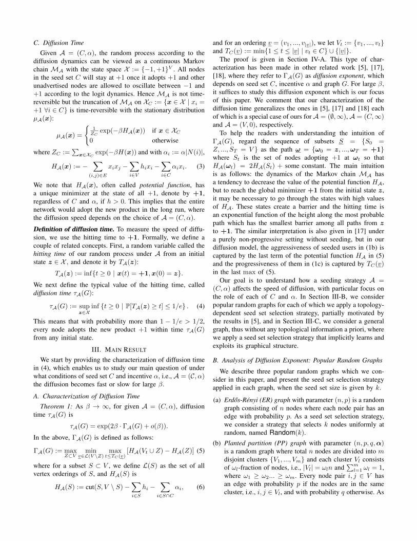
Fig. 1: A graphical summary of Theorems a, b, and c, where constants ξ∗, ξc, and ξd > 0 are defined therein.

a seed set selection strategy, we consider a cluster-basedone, named Cluster(k) that chooses a set C of size k thatis the solution of the following optimization problem:

minC′:|C′|=k

max1≤l≤m

[1− h2

ωl − δlq

p− |C

′ ∩ Vl|n

](7)

where δl :=∑l−1l′=1ωl′ −

1−h2 (1− ωl).

(c) Power law (PL) graph with parameter (n, γ) has a powerlaw degree distribution parameterized by γ ≥ 2, i.e., thefraction of nodes having degree d is proportional to d−γ .We consider the PL graph generated by the preferentialattachment with minimum degree 2 as in [27], [28].As a seed set selection strategy, we consider a degree-based one, named Degree(k), which chooses k nodes indecreasing order of their degrees.

We now present Theorem 2 which provides the asymptoticquantification of the diffusion exponents for three graphs. Foreach graph, we have two parts: part (i) provides a lower boundof the necessary size of seed set for the order-wise reduction ofthe diffusion exponent, and part (ii) provides an upper boundof the sufficient size of seed set for the same reduction. Theproof is given in Section IV-B.

Theorem 2: As n → ∞, for given α ≥ 0 and any smallconstant ε > 0, the following events occur almost surely:(a) Suppose G is an ER graph with np = ω(log n).

(i) For every seed set C such that |C|n ≤1−h2 − ε,

ΓA(G) = Θ(n2p).

(ii) If seed set C is selected by Random(k) and |C|n ≥1−h2 + ε, then

ΓA(G) =

Θ((1− h− α)np) if α ≤ 1− h− ε0 if α ≥ 1− h+ ε.

(b) Suppose G is a PP graph with (1 − αl)nq ≤ αlnp =ω(log n) and αmn = Ω(n).(i) For every C such that |C|n ≤

1−h2 − ξ∗ − ε,

ΓA(G) = Θ(n2p)

where ξ∗ := m√

qp .

(ii) If seed set C is selected by Cluster(k) and |C|n ≥

1−h2 − ξc + ε, then

ΓA(G) =

Θ((1− h− α)np) if α ≤ 1− h− ε0 if α ≥ 1− h+ ε

where ξc := (1−h)22

qp .

(c) Suppose G is a PL graph with γ > 1 and dmin = 2.(i) If C = ∅, i.e., |C| = 0, then for small enough h ≥ 0,

ΓA(G) = Ω(n)3.

(ii) If seed set C is selected by Degree(k) and |C|n ≥

1− ξd + ε, then

ΓA(G) =

O(

(1− h− α)n1γ

)if α ≤ 1− h− ε

0 if α ≥ 1− h+ ε

where ξd := 12γ(ζ(γ)−1) with ζ(γ) :=

∑∞d=1

1dγ .

In Figure 1, we graphically summarize the above theoremwhich shows a phase transition of the diffusion exponent in aninterval of the seed set size for each graph. For example, in ERgraphs, any seed set C cannot reduce the order of the diffusionexponent if |C|n ≤

1−h2 − ε. But we can reduce the order with

seed set C such that |C|n ≥1−h2 +ε. Hence, in ER graphs, the

phase transition from Θ(n2p) to Θ((1− h− α)np) occurs in[(1−h2 − ε

)n,(1−h2 + ε

)n], of which the minimum value is

a lower bound on necessary size and the maximum one is anupper bound on sufficient size for the phase transition.

Seed set size first and then incentive. We first focus on theinterpretation of Theorem 2(a) for ER graphs, where analogousinterpretation also works for PP and PL graphs. In ER graphs,it is not possible to reduce the order of the diffusion exponentby any seed set even with α =∞, if the size of seed set doesnot exceed a certain threshold, i.e., |C| < 1−h

2 n. In otherwords, it is necessary to have a seed set of size more than1−h2 n for the order-wise reduction while having large α is not

3This diffusion exponent without seeding in PL graphs was studied in [17].

necessary, i.e., we need to secure a certain number of seedsfirst instead of high incentive. However, once the size of seedset even slightly exceeds the threshold, i.e., |C| > 1−h

2 n, thereis a phase transition of the diffusion exponent from Θ(n2p)to Θ((1 − h − α)np) where only incentive α can reduce theorder of the diffusion exponent. This implies that after thephase transition, it is more efficient to increase the incentivethan to increase the seed set size. We note that α = 1 − hmakes the diffusion extremely fast, i.e., ΓA(G) = 0, since1 − h is nothing but the minimum of additional payoff thatmakes a seeded user’s best response to be adopting the newproduct regardless of its neighbors’ choice.

Selection of seed set. As we explained in the above, The-orem 2(a) shows a sharp phase transition of the diffusionexponent at the threshold of the seed size in ER graphs, wheredue to the symmetric connectivity, any arbitrary choice ofseed set C can have such phase transition at |C|n = 1−h

2 .Such narrow gap between the necessary and the sufficient sizesimplies the efficiency of Random(k) for ER graphs, which isalso shown in [5]. In Theorems 2(b) and 2(c), we also obtainsimilar phase transitions between 1−h

2 − ξ∗ <|C|n < 1−h

2 − ξcfor PP graphs and 0 < |C|

n < 1 − ξd for PL graphs. Thephase transition in PP graphs and PL graphs become sharp asthe one in ER graphs when the fraction of the inter-clusteredges decreases, i.e., q

p → 0 for PP graphs and the degreedistribution becomes more skewed, i.e., γ → ∞. Differentfrom ER graphs, for PP and PL graphs, in order to have a phasetransition, we need to carefully select seeds depending on thenetwork topology: Cluster(k) for PP graphs and Degree(k)for PL graphs.

We note that Cluster(k) is analogous to that in [5], butwe improve the previous one for a tighter phase transition,in terms of that using the previous one, |C| = 1−h

2 n isnecessary to reduce the order of the diffusion exponent, i.e.,Cluster(k) saves budget ξcn for the same purpose, where theimprovement is made by the second term in (7). The intuitionbehind Cluster(k) with (7) is collecting more seeds fromlarger clusters but with some balance between the fractionof seeds in each cluster since a larger cluster has higher1−h2 ωl − δl qp l. The PL graph is generated by the preferential

attachment mechanism, i.e., the more connected node has morelikely to receive new links. Thus connectivity is concentratedin a small number of high-degree nodes like hubs connectingother low-degree nodes. Thus it is very natural to seed thehigh degree nodes as Degree(k) does.

C. Analysis of Diffusion Exponent: General Graphs

In the previous section, we studied popular random graphsand the corresponding seeding algorithms, i.e., the arbitrary(or random) seeding for ER graphs, the cluster-based seedingfor PP graphs, and the degree-based seeding for PL graphs.To tolerate topology-sensitive performances of seeding algo-rithms, we propose a new one, called General(k), workingfor arbitrary graphs, which is inspired by those in the previoussections.

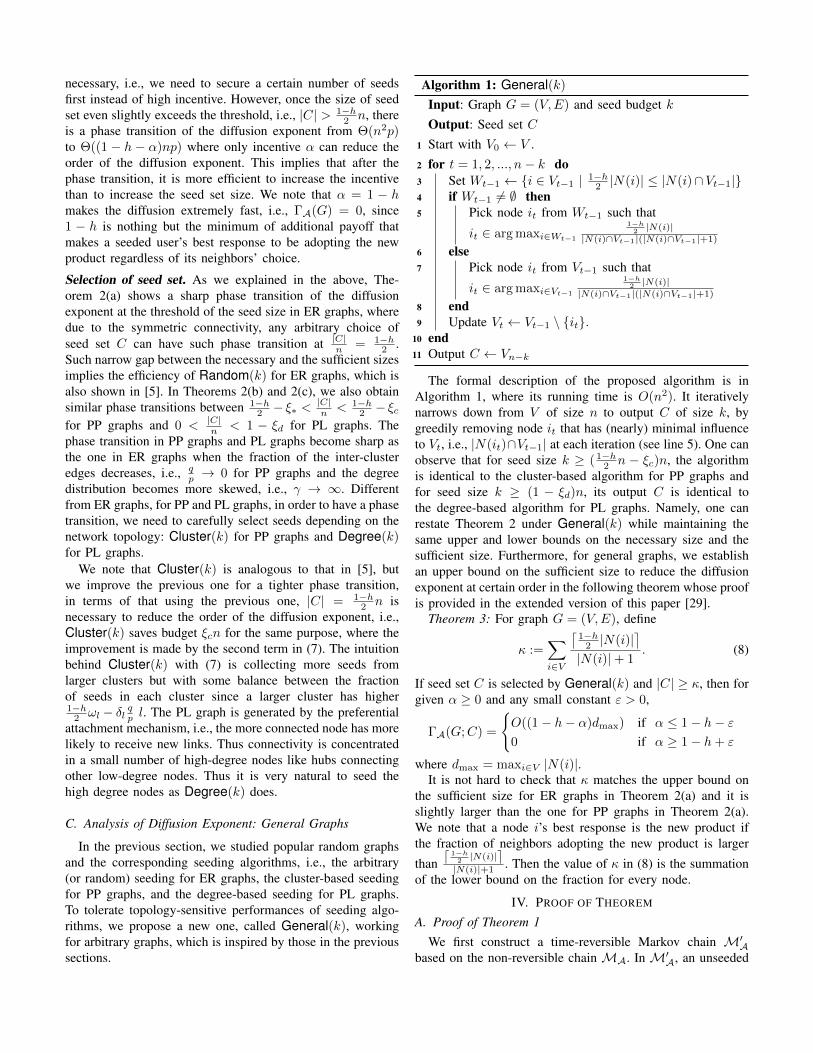
Algorithm 1: General(k)

Input: Graph G = (V,E) and seed budget kOutput: Seed set C

1 Start with V0 ← V .2 for t = 1, 2, ..., n− k do3 Set Wt−1 ← i ∈ Vt−1 | 1−h

2 |N(i)| ≤ |N(i)∩Vt−1|4 if Wt−1 6= ∅ then5 Pick node it from Wt−1 such that

it ∈ arg maxi∈Wt−1

1−h2 |N(i)|

|N(i)∩Vt−1|(|N(i)∩Vt−1|+1)

6 else7 Pick node it from Vt−1 such that

it ∈ arg maxi∈Vt−1

1−h2 |N(i)|

|N(i)∩Vt−1|(|N(i)∩Vt−1|+1)

8 end9 Update Vt ← Vt−1 \ it.

10 end11 Output C ← Vn−k

The formal description of the proposed algorithm is inAlgorithm 1, where its running time is O(n2). It iterativelynarrows down from V of size n to output C of size k, bygreedily removing node it that has (nearly) minimal influenceto Vt, i.e., |N(it)∩Vt−1| at each iteration (see line 5). One canobserve that for seed size k ≥ ( 1−h

2 n − ξc)n, the algorithmis identical to the cluster-based algorithm for PP graphs andfor seed size k ≥ (1 − ξd)n, its output C is identical tothe degree-based algorithm for PL graphs. Namely, one canrestate Theorem 2 under General(k) while maintaining thesame upper and lower bounds on the necessary size and thesufficient size. Furthermore, for general graphs, we establishan upper bound on the sufficient size to reduce the diffusionexponent at certain order in the following theorem whose proofis provided in the extended version of this paper [29].

Theorem 3: For graph G = (V,E), define

κ :=∑i∈V

⌈1−h2 |N(i)|

⌉|N(i)|+ 1

. (8)

If seed set C is selected by General(k) and |C| ≥ κ, then forgiven α ≥ 0 and any small constant ε > 0,

ΓA(G;C) =

O((1− h− α)dmax) if α ≤ 1− h− ε0 if α ≥ 1− h+ ε

where dmax = maxi∈V |N(i)|.It is not hard to check that κ matches the upper bound on

the sufficient size for ER graphs in Theorem 2(a) and it isslightly larger than the one for PP graphs in Theorem 2(a).We note that a node i’s best response is the new product ifthe fraction of neighbors adopting the new product is larger

than d1−h2 |N(i)|e|N(i)|+1 . Then the value of κ in (8) is the summation

of the lower bound on the fraction for every node.

IV. PROOF OF THEOREM

A. Proof of Theorem 1We first construct a time-reversible Markov chain M′A

based on the non-reversible chain MA. In M′A, an unseeded

node i /∈ C has the same probability of the one in (1a) buta seeded node i ∈ C has a positive probability to go back to−1 from +1, to guarantee the time-reversibility, as describedin the following:

P[si|x] =

logit(h+ α, si,x) if xi = −1

exp(−ββ′)logit(h+ α, si,x) if xi = +1

+ (1− exp(−ββ′))1+(si).

As β → ∞, the transition probability in M′A with β′ > 0converges to that in MA thus the diffusion time τ ′A ofM′A would also converge to τA. We formally obtain theconvergence of τ ′A to τA with sufficiently large β′ in thefollowing lemma whose proof is provided in the extendedversion of this paper [29].

Lemma 1: Suppose β′ ≥ 8n2. Then, as β → ∞, τ ′Aconverges to τA.

Thus, we now focus on the characterization of τ ′A(G). Todo so, for x,y ∈ X such that x and y are same except anode i, i.e., xj = yj for all j 6= i and xi = −yi, we write thestationary distribution µ′A(x) and the transition rate p′A(x,y)of M′A as µ′A(x) = exp(−βH ′A(x) + o(β)) and p′A(x,y) =exp(−βV ′A(x,y) + o(β)) where

H ′A(x) := HA(x)− β′∑i∈C

1+(xi),

V ′A(x,y) :=

[HA(y)−HA(x)]+ if i /∈ C[HA(y)−HA(x)]+ + β′1+(xi) if i ∈ C,

and for x ∈ R, [x]+ := maxx, 0. These expressions ofµ′A and p′A allow us to apply the hitting time analysis of theFreidlin-Wentzell chain, provided in Chapter 6 [30], for thetime-reversible chainM′A and we obtain the following lemmaas a corollary of Theorem 6.38 therein.

Lemma 2: As β → ∞, τ ′A = exp(βΓ′A + o(β)) whereΓ′A(G) is

minω:−1→+1

maxt′<|ω|

maxt′≤t<|ω|

[H ′A(ωt)+V ′A(ωt,ωt+1)−H ′A(ωt′)].

(9)

Here the min runs over every possible path ω from −1 to+1 such that for 0 ≤ t < |ω|, ωt and ωt+1 are same excepta node’s state.

Thus it is enough to show that for sufficiently large β′ ≥8n2 ≥ 4 maxx∈S HA(x),

Γ′A(G) = 2ΓA(G). (10)

Recalling that for z ∈ S and Z ⊂ V such that Z = i ∈V | zi = +1, HA(ωt) = 2HA(St) + some constant, we canrewrite ΓA(G) in (5) as follows:

2ΓA(G) = maxz 6=+1

minω:[z→+1]V

maxt≤TC(ω)

[HA(ωt)−HA(z)] (11)

where for a subset S ⊂ V , we let [z → +1]S denote theset of every possible path ω from z to +1 such that for alli ∈ S and 0 ≤ t′ ≤ t < |ω|, ωt,i = +1 if ωt′,i = +1 andwe let TC(ω) := min1 ≤ t < |ω| | ∃i ∈ C s.t. ωt−1,i =−1 and ωt,i = +1 ∪ |ω|.

To show (10), we will rewrite the optimization in (9) as theone in (11). Suppose ω /∈ [−1→ +1]C . Then there exists ssuch that ωs,i = +1 and ωs+1,i = −1. Thus it follows that

maxt′<|ω|

maxt′≤t<|ω|

[H ′A(ωt) + V ′A(ωt,ωt+1)−H ′A(ωt′)]

≥ V ′A(ωs,ωs+1) ≥ β′,

which implies that we can reduce the search space of the minin (9) to [−1→ +1]C when β′ is sufficiently large.

Suppose ω ∈ [−1→ +1]C and there exists T < |ω| suchthat for some i ∈ C, ωT−1,i = −1 and ωT,i = +1. Then forall t, t′ such that t′ ≤ T < t, it follows that

H ′A(ωt) + V ′A(ωt,ωt+1)−H ′A(ωt′)

= HA(ωt) + [HA(ωt+1)−HA(ωt)]+ −HA(ωt′)

− β′∑i∈C

(1+(ωt,i)− 1+(ωt′,i))

which is less than − 12β′ since 1+(ωt,i) − 1+(ωt′,i) ≥ 1 and

β′ ≥ 4 maxx∈S HA(x). Thus, for sufficiently large β′, we canreduce the search space of the last max in (9) and we obtain

Γ′A(G) = minω:[−1→+1]C

maxt′<|ω|

maxt′≤t<TC(ω)

[HA(ωt)−HA(ωt′)]

where TC(ω) := min1 ≤ t < |ω| | ∃i ∈ C s.t. ωt−1,i =−1 and ωt,i = +1 ∪ |ω|. Furthermore, we can reduce thesearch space of the min from [−1→ +1]C to [−1→ +1]Vby similar argument with the submodularity of HA(S) usedfor the proof of Theorem 2 in [17]. This completes the proof.

B. Proof of Theorem 2

To prove Theorems 2(a)-(c) for different graphs and seedselections, we will use the following upper and lower boundson ΓA(G), whose proof is presented in the extended versionof this paper [29].

Theorem 4 (Exponent Bound): For given G and seed set C,we define Γ(C) as follows:

Γ(C) := maxC⊂Z⊂V

minv∈L(V \Z)

max1≤t≤|v|

[H(Vt ∪ Z)−H(Z)] . (12)

where for a subset S ⊂ V , H(S) is the value of HA(S) withα = 0. Then, for A = (C,α), if follows that

max

Γ(C), min

i∈V(1− h− α)|N(i)|

≤ ΓA(G) ≤ max

Γ(C), max

i∈C(1− h− α)|N(i)|

(13)

(14)

However, handling Γ(C) directly in the above theorem ishard in general. So, we establish the following key lemmasthat provide criteria to check if Γ(C) is large or small, i.e.,Γ(C) ≥ δ or Γ(C) = 0, where the proofs are provided in theextended version of this paper [29].

Lemma 3: Consider graph G = (V,E) and seed set C.Suppose that for a given k such that |V \C| ≤ k ≤ |V |, thereexists a constant δ > 0 such that for every subset S ⊂ V \ Cwith |S| = k,

(1− h) · cut(S, V \ S)− 2 · cut(S,C)− 2h · edge(S)

= H(S ∪ C)−H(C) ≥ δ, (15)

where edge(S) is the number of edges between nodes in S,i.e., edge(S) = |(i, j) ∈ E | i, j ∈ S|. Then we haveΓ(C) ≥ 2δ.

Lemma 4: Consider graph G = (V,E) and seed set C.Suppose there exists a sequence s of nodes in V \C such thatfor all t = 1, ..., |V \ C|,(1− h)|N(st)| − 2|N(st) ∩ St−1| = H(St)−H(St−1) ≤ 0

(16)where St = C ∪ s1, ..., st. Then we have Γ(C) = 0.

1) Proof of Theorem 2(a): Recalling ER graph G = (V,E)in Theorem 2(a), we note that ε2np = ω(log n). Using theChernoff inequality and the union bound, it follows that

P

[⋂i∈V

[∣∣|N(i)| − np∣∣ ≤ ε

2np]]≥ 1−O(n exp(−ε2np)),(17)

where the last term converges to 1 as n→∞ due to ε2np =ω(log n). Then for large n, it follows that |N(i)| = Θ(np) andΓ(G;C) = O(n2p) due to (12) with H(S) ≤ (1 + 2h)|E| =Θ(n2p). Then using the above observations and Theorem 4,the proof is completed if the following events occur with highprobability:

Γ(C) =

Ω(n2p) if |C|n ≤

1−h2 − ε, (18)

0 if |C|n ≥1−h2 + ε. (19)

Due to space limitation, we provide the proofs of (18) and (19)without details which are provided in the extended version ofthis paper [29]. Suppose |C|n ≤ 1−h

2 − ε. Then, using theChernoff inequality and the union bound, it is not hard tocheck that for every S ⊂ V \ C such that |S|n = ε

2 , thevalues of cut(S, V \ S), cut(S,C), and edge(S) concentratesat ε

2

(1− ε

2

)n2p, ε

2

(1−h2 − ε

)n2p, and ε2

8 n2p, respectively,

as n → ∞, so that H(S ∪ C) − H(C) ≥ ε2

8 n2p with high

probability. With Lemma 3, this completes the proof of (18).Suppose |C|n ≥

1−h2 + ε. Then, using the Chernoff bound

and the union bound, it is not hard to check that for everynode i ∈ V \ C, (1 − h)|N(i)| − 2|N(i) ∩ C| ≤ − ε2np withhigh probability. With Lemma 4, this completes the proofs of(19) and Theorem 2(a).

2) Proof of Theorem 2(b): Due to space limitation, weprovide a sketch of the proof with q = 0. The rigorousproof with q > 0 is provided in the extended version ofthis paper [29]. Suppose q = 0, i.e., the PP graph G is m-disjoint ER graphs, G1 = (V1, E1), ..., Gm = (Vm, Em).Let Cl := Vl ∩ C. Then, from Lemma 4.3 in [5], it followsthat

Γ(G;C) = maxl=1,...,m

Γ(Gl;Cl). (20)

If |C|n ≤1−h2 − ε, there must exist l′ such that C

n ≤1−h2 −

εωm, i.e., from Theorem 2(a), Γ(Gl′ ;Cl′) = Θ(n2p). Using(20), this completes the proof of part (i) in Theorem 2(b).In addition, if |C|n ≤ 1−h

2 − ε and seed set C is selectedby Cluster(k), i.e., C is the solution of (7), then for all l,Cn ≥

1−h2 +εωm, i.e., from Theorem 2(a), Γ(Gl;Cl) = Θ((1−

h−α)np). Using (20), this completes the proof of part (ii) inTheorem 2(b).

(a) PPfacebook graph (b) PLfacebook graph

Fig. 2: (a) PPfacebook [31]: 4039 nodes and 88234 edgesand (b) PLfacebook [32]: 1899 nodes and 13838 edges

3) Proof of Theorem 2(c): Let S be the subset of nodeswith degree two. Then for large n, the fraction of S is |S|n =

12γ(ζ(γ)−1) . Hence the seed set C selected by Degree(k)

with k ≥ (1 − ξd)n, includes all nodes with degree three ormore, i.e., V \ C ⊂ S. Since G is connected, there existsa linear ordering s of S such that for all t = 1, ..., |S|,|N(st)∩St| ≥ 1, where St = C ∪s1, ..., st−1. This impliesthat the linear ordering s satisfies (16). Thus Lemma 4 with(16) shows Γ(C) = 0. We note that the maximum degreeof G is O(n1/γ), since the number of nodes with degreeω(n1/γ) is nf(n1/γ) = o(n(n1/γ)−γ) = o(1). Thus the proofof Theorem 2(c) is completed by Theorem 4 with Γ(C) = 0and dmax = O(n1/γ).

V. NUMERICAL RESULTS

In this section, we provide simulation results based on somereal social networks that demonstrate our theoretical findings.

Setup. We use two data set of the social network amongFacebook users, represented as two undirected graphs, whereeach node corresponds to a Facebook account and each edgerepresents Friend Lists of Facebook. We name the graph from[31] PPfacebook, and the graph from [32] PLfacebook,whose graphical presentations are given in Figures 2(a) and2(b), respectively. As hinted from the names of two graphsand Figure 2, a clustering structure is more observed inPPfacebook, whereas a skewed degree distribution (whichturns out to be a power law) is prominent in PLfacebook.4

We choose β = 10 for the degree of rationality and useh = 0.5 for the payoff difference between the new and oldproducts. We estimate the hitting time to +1 for General(k)with varying seed set size k and diverse incentive α in each ofPPfacebook and PLfacebook, where our results are averagedover 100 random samples.

Results. We plot the diffusion times in PPfacebook andPLfacebook in Figures 3(a) and 3(b), respectively, wherefor brevity, we omit the results with α > 0.5 since thecurve doesn’t change much for α > 0.5. As we analyzedin Section III, if the seed set size is less than a certain

4Our calculation reveals that the clustering coefficients of PPfacebook andPLfacebook are 0.617 and 0.1385, respectively, and the degree distributionsof those two graphs are fit into power law distributions with exponent γ =1.18 and 1.344, respectively.

α = 0.47

α = 0.48

α = 0.49

α ≥ 0.50

Dif

fusio

n T

ime τ

0

50

100

150

200

Seed Set Size k

0 1000 2000 3000 4000

(a) Diffusion time in PPfacebook

α = 0.47

α = 0.48

α = 0.49

α ≥ 0.50

Dif

fusio

n T

ime τ

0

50

100

150

200

Seed Set Size k

0 500 1000 1500

(b) Diffusion time in PLfacebook

Fig. 3: Diffusion time in PPfacebook and PLfacebook forα = 0.5, 0.49, 0.48, 0.47 with varying seed size

value, which is 190 and 30 in PPfacebook and PLfacebook,respectively, the diffusion time is not reduced by increasingincentive α more than 0.5, while if the seed set size is suffi-ciently large, the diffusion time is dramatically decreased by aslight increment of incentive α from 0.47 to 0.5. ComparingFigures 3(a) and 3(b), the diffusion time reduction by incentiveα in PPfacebook is more significant than the reduction inPLfacebook. Such topology-dependent impact of incentiveα is analogous to our analysis of the diffusion exponentsin PP and PL graphs, each of which is Θ((1 − h − α)np)and O((1 − h − α)n1/γ), respectively, where n n1/γ . Wecomment that the above tendencies are similarly observed withdifferent choice of parameters β and h, which are omitted dueto space limitation.

VI. CONCLUSION

We model an important feature of seeded users who adjustthe degree of their willingness to diffusion depending on howmuch incentive is given. In our model, our main questionis how many seeds, i.e., quantity, and how much incentive,i.e., quality, are necessary and sufficient for accelerating thediffusion significantly. We found the phase transition of thediffusion time between the necessary and sufficient seed setsizes. Our results imply that after seeding a certain numberof individuals, it is better to give more incentives to alreadyselected seeded people instead of making efforts on seedingnew ones.

REFERENCES

[1] M. Richardson and P. Domingos, “Mining knowledge-sharing sites forviral marketing,” in Proc. of ACM SIGKDD, 2002.

[2] D. Kempe, J. Kleinberg, and E. Tardos, “Maximizing the spread ofinfluence through a social network,” in Proc. of ACM SIGKDD, 2003.

[3] S. Morris, “Contagion,” The Review of Economic Studies, vol. 67, no. 1,pp. 57–78, 2000.

[4] W. Chen, C. Wang, and Y. Wang, “Scalable influence maximization forprevalent viral marketing in large-scale social networks,” in Proc. ofACM SIGKDD, 2010.

[5] J. Ok, Y. Jin, J. Shin, and Y. Yi, “On maximizing diffusion speed insocial networks: impact of random seeding and clustering,” in Proc. ofACM SIGMETRICS, 2014.

[6] R. M. Anderson and R. M. May, Infectious Diseases of Humans. OxfordUniversity Press, 1991.

[7] N. T. J. Bailey, The Mathematical Theory of Infectious Diseases and ItsApplications. Hafner Press, 1975.

[8] N. Du, L. Song, M. Gomez-Rodriguez, and H. Zha, “Scalable influenceestimation in continuous-time diffusion networks,” in Proc. of NIPS,2013.

[9] J. Kleinberg, “Cascading behavior in networks: Algorithmic and eco-nomic issues,” Algorithmic Game Theory, pp. 613–632, 2007.

[10] A. Ganesh, L. Massouli, and D. Towsley, “The effect of networktopology on the spread of epidemics,” in Proc. of IEEE Infocom, 2003.

[11] S. Banerjee, A. Chatterjee, and S. Shakkottai, “Epidemic thresholds withexternal agents,” in Proc. of IEEE INFOCOM, 2014.

[12] S. Krishnasamy, S. Banerjee, and S. Shakkottai, “The behavior ofepidemics under bounded susceptibility,” in The 2014 ACM internationalconference on Measurement and modeling of computer systems. ACM,2014, pp. 263–275.

[13] M. Kandori, G. J. Mailath, and R. Rob, “Learning, mutation, and longrun equilibria in games,” Econometrica, vol. 61, no. 1, pp. 29–56, Jan.1993.

[14] G. Ellison, “Learning, local action, and coordination,” Econometrica,vol. 61, no. 5, pp. 1047–1071, Sep. 1993.

[15] H. P. Young, Individual strategy and social structure: An evolutionarytheory of institutions. Princeton University Press, 1998.

[16] E. Coupechoux and M. Lelarge, “Impact of clustering on diffusions andcontagions in random networks,” in Proc. of IEEE NetGCooP, 2011.

[17] A. Montanari and A. Saberi, “Convergence to equilibrium in localinteraction games,” in Proc. of IEEE FOCS, 2009.

[18] J. Ok, J. Shin, and Y. Yi, “On the progressive spread over strategicdiffusion: Asymptotic and computation,” in Proc. of IEEE INFOCOM,2015.

[19] A. Fazeli, A. Ajorlou, and A. Jadbabaie, “Optimal budget allocation insocial networks: Quality or seeding?” in Decision and Control (CDC),2014 IEEE 53rd Annual Conference on. IEEE, 2014, pp. 4455–4460.

[20] E. Ackerman, O. Ben-Zwi, and G. Wolfovitz, “Combinatorial model andbounds for target set selection,” Theoretical Computer Science, vol. 411,no. 44, pp. 4017–4022, 2010.

[21] D. Reichman, “New bounds for contagious sets,” Discrete Mathematics,vol. 312, no. 10, pp. 1812–1814, 2012.

[22] A. Coja-Oghlan, U. Feige, M. Krivelevich, and D. Reichman, “Conta-gious sets in expanders,” in Proc. of SODA. ACM–SIAM, 2015, pp.1953–1987.

[23] D. McFadden, Chapter 4: Conditional logit analysis of qualitative choicebehavior in Frontiers in Econometrics. Academic Press, New York,1973.

[24] D. Mookherjee and B. Sopher, “Learning behavior in an experimentalmatching pennies game,” Games and Economic Behavior, vol. 7, no. 1,pp. 62–91, 1994.

[25] R. D. McKelvey and T. R. Palfrey, “Quantal response equilibria fornormal form games,” Games and Economic Behavior, vol. 10, no. 1,pp. 6–38, 1995.

[26] L. E. Blume, “The statistical mechanics of strategic interaction,” Gamesand Economic Behavior, vol. 5, no. 3, pp. 387–424, 1993.

[27] M. Mihail, C. Papadimitriou, and A. Saberi, “On certain connectivityproperties of the internet topology,” in Proc. of IEEE FOCS, 2003.

[28] C. Gkantsidis, M. Mihail, and A. Saberi, “Conductance and congestionin power law graphs,” ACM SIGMETRICS Performance EvaluationReview, vol. 31, no. 1, pp. 148–159, 2003.

[29] https://dl.dropboxusercontent.com/u/65914625/paper files/SocialSpread/INFOCOM17 Incentive full.pdf.

[30] E. Olivieri and M. E. Vares, Large Deviations and Metastability.Cambridge University Press, 2005.

[31] J. McAuley and J. Leskovec, “Learning to discover social circles in egonetworks,” in Proc. of NIPS, 2012.

[32] T. Opsahl and P. Panzarasa, “Clustering in weighted networks,” Socialnetworks, vol. 31, no. 2, pp. 155–163, 2009.