Incidence and Distributional Effects of Value Added Taxes * Ingvil Gaarder † This version: September 2016 Abstract: Much of the controversy surrounding recent policy proposals to broaden the base for value added taxes (VAT) revolves around who ultimately bears the burden of these taxes. The typical assumption is that consumer prices fully reflect taxes, so that the main empirical question is how the tax induced price changes affect members of different income groups. However, the evidence base is scarce and market imperfec- tions could generate both over and under-shifting of VAT to consumer prices. In this paper, we examine the incidence and distributional effects of VAT in a setting with plausibly exogenous variation in tax rates. The context of our study is a sharp change in the VAT policy on food items in Norway. Using a regression discontinuity design, we examine the direct impact of the policy change on the consumer prices of food items as well as any cross-price effects on other goods. Our estimates suggest that taxes levied on food items are completely shifted to consumer prices, whereas the pricing of other goods is not materially affected. To understand the distributional effects of the VAT reform, we use expenditure data and estimate the compensating variation of the tax induced price changes. We find that lowering the VAT on food attenuates inequality in consumer welfare, in part because households adjust their spending patterns in re- sponse to the price changes. By comparison, the usual first order approximation of the distributional effects, which ignores behavioral responses, seriously understates the redistributive nature of the VAT reform. Keywords: Value added taxes; incidence; distributional effects; pass-through Jel Codes: H20, H22, H23, H31, H32. * Thanks to Jerome Adda, Russel Cooper, Guy Michaels, Magne Mogstad, Kjell G. Salvanes and Fredrik Wulfsberg for helpful comments and suggestions. I also wish to than the Norwegian Social Science Data Service together with Norges Bank for providing the Consumer Expenditure Survey Data and the Consumer Price Index Data, respectively. † University of Chicago. Email: [email protected]
Transcript
Incidence and Distributional Effects of Value AddedTaxes∗
Ingvil Gaarder†
This version: September 2016
Abstract: Much of the controversy surrounding recent policy proposals to broadenthe base for value added taxes (VAT) revolves around who ultimately bears the burdenof these taxes. The typical assumption is that consumer prices fully reflect taxes, sothat the main empirical question is how the tax induced price changes affect membersof different income groups. However, the evidence base is scarce and market imperfec-tions could generate both over and under-shifting of VAT to consumer prices. In thispaper, we examine the incidence and distributional effects of VAT in a setting withplausibly exogenous variation in tax rates. The context of our study is a sharp changein the VAT policy on food items in Norway. Using a regression discontinuity design, weexamine the direct impact of the policy change on the consumer prices of food items aswell as any cross-price effects on other goods. Our estimates suggest that taxes leviedon food items are completely shifted to consumer prices, whereas the pricing of othergoods is not materially affected. To understand the distributional effects of the VATreform, we use expenditure data and estimate the compensating variation of the taxinduced price changes. We find that lowering the VAT on food attenuates inequalityin consumer welfare, in part because households adjust their spending patterns in re-sponse to the price changes. By comparison, the usual first order approximation ofthe distributional effects, which ignores behavioral responses, seriously understates theredistributive nature of the VAT reform.Keywords: Value added taxes; incidence; distributional effects; pass-throughJel Codes: H20, H22, H23, H31, H32.
∗Thanks to Jerome Adda, Russel Cooper, Guy Michaels, Magne Mogstad, Kjell G. Salvanes andFredrik Wulfsberg for helpful comments and suggestions. I also wish to than the Norwegian SocialScience Data Service together with Norges Bank for providing the Consumer Expenditure Survey Dataand the Consumer Price Index Data, respectively.
Are taxes levied on commodities completely shifted to consumer prices, or does theincidence also fall on firms? What are the welfare implications of commodity taxes forpoor and rich households? These questions are important for both policy and scientificresearch, as commodity taxes make up a large part of fiscal revenue in most developedcountries. In Europe, much of the controversy surrounding recent policy proposals tobroaden the base for value added taxes (VAT) revolves around who ultimately bears theburden of these taxes. In the United States, recent debates on whether to increase re-liance on consumption-based taxes have raised concerns over the distributional effectsof such policy changes. The typical assumption is that consumer prices fully reflecttaxes, so that main important empirical question is how the tax induced price changesaffect members of different income groups. However, the evidence base is scarce (Craw-ford, Keen, and Smith, 2010) and market imperfections could generate both over andunder-shifting of commodity taxes to consumer prices (Seade, 1987; Delipalla and Keen,1992; Anderson, De Palma, and Kreider, 2001).
The aim of this paper is to investigate the incidence and distributional effects ofcommodity taxes in a setting with plausibly exogenous variation in tax rates. Thecontext of our study is an abrupt change in the VAT policy on food in Norway. As inmost European countries, food retailing in Norway is highly concentrated with a fewchains commanding most of the market. On July 1st, 2001 the Norwegian governmentreduced the VAT on all food items from 24 to 12 percent, while the VAT on non-fooditems remained at 24 percent. This sharp change in VAT policy provides an attractivesetting to analyze the pass-through of commodity taxes using a regression discontinuity(RD) design that compares consumer prices just before (i.e. the control group) and after(i.e. the treatment group) the reform date. We apply this design to rich data on retailprices for a representative sample of consumer goods. This allows us to estimate thedirect impact of the policy change on the consumer prices of food items as well as anycross-price effects on other goods. We challenge the identifying assumptions of the RDdesign through a number of robustness checks, finding little cause for worry.
The RD estimates tell us whether the gains from the VAT reform ultimately fall onconsumers or producers. However, the distributional effects also depend on the extentto which poor and rich households are affected by the pass-through to consumer prices.Using survey data on consumer expenditure, we perform a first order approximation ofthe distributional effects. An advantage of this approach is that it simply requires infor-
1
mation on the price changes and the pre-reform expenditure patterns of the households.However, the VAT reform generated substantial rather than marginal changes in foodprices. In such cases, substitution effects can be non-trivial, as consumers substitutetowards relatively cheaper goods. The first order approximations ignore these effects,and therefore, can be seriously biased (see e.g. Banks, Blundell, and Lewbel, 1996).To address this concern, we use expenditure data to estimate the Almost Ideal (AI)demand system. This allows us to incorporate behavioral responses in estimating thecompensating variation of the changes in prices associated with the VAT reform.
The insights from our empirical results may be summarized with two broad conclu-sions. First, the VAT on food items is completely shifted to consumer prices, implyingthat producers bear little, if anything, of the tax burden. By comparison, there is littleif any spillover effects of the VAT reform to the consumer prices of non-food items.Second, lowering the VAT on food substantially attenuates inequality in consumer wel-fare. This reduction in inequality is partly because poor households have a higherexpenditure share on food prior to the reform, but also because households adjusttheir spending patterns in response to prices changes. By comparison, the usual firstorder approximation of the distributional effects, which ignores behavioral responses,seriously understates the redistributive nature of the VAT reform.
Our findings have implications for recent proposals for tax reforms. For example, theMirrlees Review (2012) sets out a comprehensive proposal for tax reform in the UnitedKingdom. A key element of the reform package is to broaden the base for VAT, inpart by removing the zero rating for food. Arguing that there is little hard evidence todraw on, the Mirrlees Review assumes the incidence of VAT is fully on consumer prices.Atkinson (2013) questions the reform proposal, stressing that until direct evidence isavailable, “we should remain agnostic about the strength of the optimal tax argumentfor extending VAT to food” (p. 6). Our paper helps to close that gap by providingtransparent and credible identification of the incidence of VAT taxes on food.
Our paper is primarily related to two recent empirical studies on the incidence ofVAT. Carbonnier (2007) studies two VAT reforms in France which reduced the rates onnew car sales and on housing repair services. He uses the variation in consumer pricesacross goods and over time to estimate the pass-through of these VAT reforms. Hisestimates suggest a majority of the tax burden is paid by consumers, especially in thecompetitive market for housing repair services. Kosonen (2013) analyze the incidenceof VAT in the context of hairdressing services in Finland. He uses a difference-in-differences strategy where the control group consists of beauty salons, day spas and
2
massage services. His estimates suggest the tax burden on hairdressing services isshared between consumers and producers.
Our paper expands on this research in several important ways. First, our studyprovides novel evidence on the incidence of a VAT tax system with lower rates on per-ceived necessities such as food. Second, our data allows us to look at cross-price effectson other goods, and therefore, capture the entire change in the price structure. Third,we quantify the extent to which a lower VAT rate on food redistributes resources frombetter-off households to less well-off households. To the best of our knowledge, sub-stitution effects have not been incorporated in distributional analysis of VAT reforms.We do so here, and investigate the accuracy of the usual first order approximation towelfare implications of tax reforms.
Our paper is also related to a sparse empirical literature on the pass-through ofsales taxes. Unlike VAT, a sales tax is imposed only at the retail level, which couldhave important implications for how the tax burden is shared between consumers andproducers (see e.g. Anderson, De Palma, and Kreider, 2001). Poterba (1996) andBesley and Rosen (1999) examined tax shifting in the United States by comparing localsales taxes and consumer prices across areas and over time. Their estimates suggestthat consumers tend to pay for sales taxes. In addition, researchers have examinedthe incidence of per unit (excise) taxes on goods such as tobacco, alcoholic beverages,and gasoline.1 Economic theory predicts that in markets with imperfect competition,the consumer share of excise taxes could differ from that of VAT. This theoreticalprediction is supported by the empirical evidence in Delipalla and O’Donnell (2001)and Carbonnier (2013).
The remainder of the paper proceeds as follows. In Section 2, we describe our dataand discuss the VAT reform and its expected impact. In Section 3, we discuss the RDdesign, present our main findings on VAT incidence, and reports robustness checks. InSection 4, we present the demand system and analyze the distributional effects of VAT.Section 5 concludes.
1For example, Doyle and Samphantharak (2008) and Marion and Muehlegger (2011) study taxincidence on gasoline. Their findings point to a complete pass-through to consumer prices. Otherstudies have examined the consumer share of excise taxes on tobacco and alcohol beverages (see e.g.Young and Bielińska-Kwapisz, 2002, Kenkel, 2005 and DeCicca, Kenkel, and Liu, 2013).
3
Table 1: Summary Statistics of Consumer Price Data
Consumer price in USD Number ofAverage St. dev Items Retailers Obs.
Food 4.21 5.50 250 545 180,510Clothing 44.30 66.96 104 522 43,380Services 15.77 39.40 33 365 22,253HH fuels 186.90 263.12 25 328 19,959Alcohol 4.96 3.68 11 388 19,700Transport 50.46 115.01 28 377 33,493Other non-durables 29.43 109.23 242 1341 126,301Notes: This table displays summary statistics for non-durable goods in 2001. In each category, the average consumerprice is computed as the weighted average of the retail prices on the items that belong to this category. We follow theprocedure used to construct the Consumer Price Index in the choice of weights and classification of items. The averageconsumer price is listed in USD, where 1 USD = 8.988 NOK.
2 Data and Background
2.1 Data sources and summary statistics
Our analysis uses two data sources. The first is a rich data set on retail prices for arepresentative sample of consumer goods. The data is collected by Statistics Norwayand forms the basis for calculating the Norwegian Consumer Price Index (CPI). Everymonth, Statistics Norway collects information about the consumer prices on a varietyof items. The reported consumer price is the current price on the 15th of each monthand the retailers report this price the first business day after the 15th. In 2001, therewere more than 180,000 recorded prices from a total of 545 different retailers. Becauseof the detailed nature of the data, it is possible to follow prices on a given item andretailer over time.
Table 1 displays summary statistics for the major consumer goods in 2001. Thistable shows that the food category consist of 250 different items. In each category, theaverage consumer price is computed as the weighted average of the retail prices on theitems that belong to this category. We follow the procedure used to construct the CPIin the choice of weights and classification of items. For food, the average consumerprice is 4 USD per item. In general, we see that the consumer prices vary considerablywithin and between the different types of goods.
The other data source we will be using is the Norwegian Consumer ExpenditureSurvey for the years 1989–2001. In addition to detailed information on each household’sexpenditure, there is also a rich set of household characteristics, including information
4
on household size, age of the household members, gender, marital status, region, laborstatus, occupation, and household disposable income. We use the same classificationof goods for the expenditure data as for the price data. Following Blundell, Pashardes,and Weber (1993), our sample consists of households in which the household head isbetween 20 and 60 years old and not self-employed; the sample is top and bottomcoded at the 99th and 1st percentile level of the distribution of household income.2
Throughout the paper, we use sampling weights to produce representative estimatesfor the corresponding population of households.
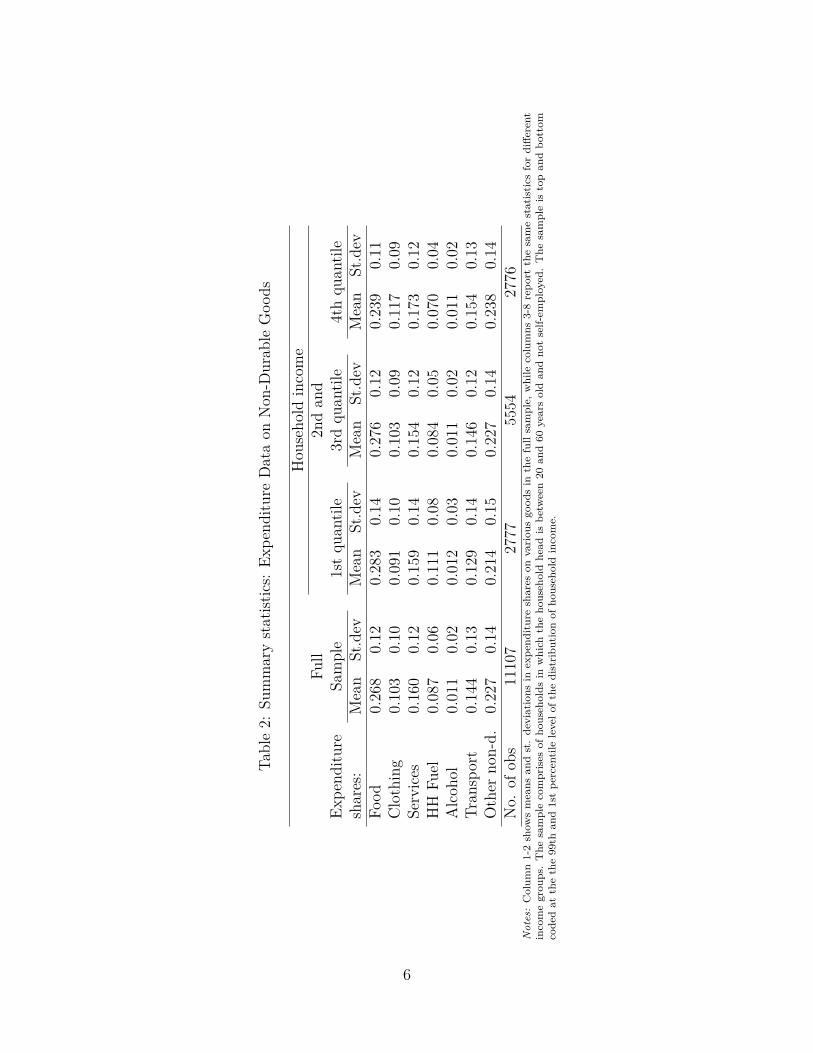
Table 2 summarizes the expenditure shares for non-durable goods. As expected,food purchases form the largest share of household expenditure and the expenditureshare declines in household income. For example, food purchases make up 28.3 % ofhousehold expenditure in the bottom quartile of the household income distributions,whereas the expenditure share on food is only 23.9 % in the top quartile. We see thesame pattern for other perceived necessities such as household fuel, while the shareof household expenditure on goods like clothing and transport increases in householdincome.
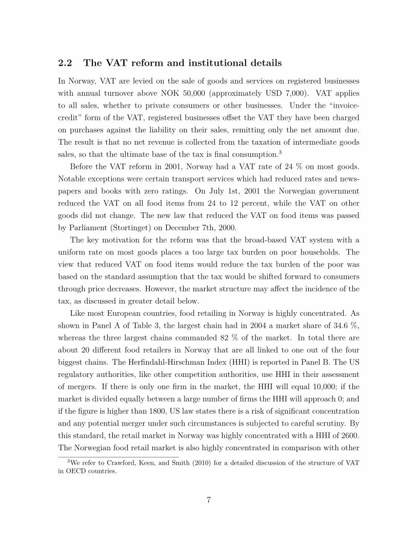
Figure 1 looks closer at the relationship between household income and food expen-diture by graphing the Engel curve. This figure provides a nonparametric description ofthe Engel curve and suggests that a log-linear specification approximates well the foodshare curve. This result aligns well with previous evidence from developed countries(see e.g. Banks, Blundell, and Lewbel, 1997).
2The top and bottom coding reduces the likelihood that outliers create nonlinearities in the budget-share equations.
5
Table2:
Summarystatist
ics:
Expe
nditu
reDataon
Non
-Durab
leGoo
ds
Hou
seho
ldincome
Full
2ndan
dEx
pend
iture
Sample
1stqu
antile
3rdqu
antile
4thqu
antile
shares:
Mean
St.dev
Mean
St.dev
Mean
St.dev
Mean
St.dev
Food
0.268
0.12
0.283
0.14
0.276
0.12
0.239
0.11
Clothing
0.103
0.10
0.091
0.10
0.103
0.09
0.117
0.09
Services
0.160
0.12
0.159
0.14
0.154
0.12
0.173
0.12
HH
Fuel
0.087
0.06
0.111
0.08
0.084
0.05
0.070
0.04
Alcoh
ol0.011
0.02
0.012
0.03
0.011
0.02
0.011
0.02
Tran
sport
0.144
0.13
0.129
0.14
0.146
0.12
0.154
0.13
Other
non-d.
0.227
0.14
0.214
0.15
0.227
0.14
0.238
0.14
No.
ofob
s11107
2777
5554
2776
Not
es:Colum
n1-2show
smeans
andst.deviations
inexpe
nditureshares
onvariou
sgo
odsin
thefullsample,
while
columns
3-8repo
rtthesamestatistics
fordiffe
rent
incomegrou
ps.The
samplecomprises
ofho
useholds
inwhich
theho
useholdhead
isbe
tween20
and60
yearsoldan
dno
tself-em
ployed.The
sampleis
topan
dbo
ttom
code
dat
thethe99th
and1stpe
rcentile
levelo
fthe
distribu
tion
ofho
useholdincome.
6
2.2 The VAT reform and institutional details
In Norway, VAT are levied on the sale of goods and services on registered businesseswith annual turnover above NOK 50,000 (approximately USD 7,000). VAT appliesto all sales, whether to private consumers or other businesses. Under the “invoice-credit” form of the VAT, registered businesses offset the VAT they have been chargedon purchases against the liability on their sales, remitting only the net amount due.The result is that no net revenue is collected from the taxation of intermediate goodssales, so that the ultimate base of the tax is final consumption.3
Before the VAT reform in 2001, Norway had a VAT rate of 24 % on most goods.Notable exceptions were certain transport services which had reduced rates and news-papers and books with zero ratings. On July 1st, 2001 the Norwegian governmentreduced the VAT on all food items from 24 to 12 percent, while the VAT on othergoods did not change. The new law that reduced the VAT on food items was passedby Parliament (Stortinget) on December 7th, 2000.
The key motivation for the reform was that the broad-based VAT system with auniform rate on most goods places a too large tax burden on poor households. Theview that reduced VAT on food items would reduce the tax burden of the poor wasbased on the standard assumption that the tax would be shifted forward to consumersthrough price decreases. However, the market structure may affect the incidence of thetax, as discussed in greater detail below.
Like most European countries, food retailing in Norway is highly concentrated. Asshown in Panel A of Table 3, the largest chain had in 2004 a market share of 34.6 %,whereas the three largest chains commanded 82 % of the market. In total there areabout 20 different food retailers in Norway that are all linked to one out of the fourbiggest chains. The Herfindahl-Hirschman Index (HHI) is reported in Panel B. The USregulatory authorities, like other competition authorities, use HHI in their assessmentof mergers. If there is only one firm in the market, the HHI will equal 10,000; if themarket is divided equally between a large number of firms the HHI will approach 0; andif the figure is higher than 1800, US law states there is a risk of significant concentrationand any potential merger under such circumstances is subjected to careful scrutiny. Bythis standard, the retail market in Norway was highly concentrated with a HHI of 2600.The Norwegian food retail market is also highly concentrated in comparison with other
3We refer to Crawford, Keen, and Smith (2010) for a detailed discussion of the structure of VATin OECD countries.
7
Figure 1: Nonparametric Engel Curve for Food Shares
0
.1
.2
.3
.4
Foo
d S
hare
s
10 11 12 13 14Log of Total Expenditure
Notes: The solid line shows the estimated relationship between the expenditure share on food and total householdexpenditure. The relationship is estimated using a nonparametric kernel regression with Gaussian kernel and a meanintegrated squared-error optimal smoothing parameter. Household expenditure is defined as yearly total expenditureon non-durables. The shaded area shows the 95 % confidence bands. Sample: households in which the household headis between 20 and 60 years old and not self-employed. The sample is top and bottom coded at the the 99th and 1stpercentile level of the distribution of household income.
countries: Einarsson (2007) reports HHI figures of 1600 in France and Germany, 1800in the United Kingdom, and as low as 300–500 in Spain.
2.3 Expected reform effects
As in the Mirrlees Review, it is customary to think of the burden of VAT as being borneby consumers in the form of higher after-tax prices, but in theory there is considerablescope for shifting of the tax burden. Indeed, there are plausible circumstances in whichconsumers bear more than 100 % of the burden or pay little if anything of the VAT.Below, we describe the measures of tax shifting we will use and briefly discuss thechallenges to making informative theoretical predictions of the pass-through of theVAT reform.
Tax shifting measures. Let τ denote the VAT rate. The producer (or pre-tax)price is p
1+τ where p is the consumer (or after-tax) price. The amount of taxes paid perunit sold is τp
1+τ . After a change in the VAT rate, the consumer price variation is dpdτ
andthe tax variation is d
dτ
(τp
1+τ
). The consumer share of the change in VAT is then given
8
Table 3: Concentration in the Food Retail Market in Norway, 2004
Panel A: Largest chain Second largest chain Third largest chain
Market share: 34.7 % 23.7 % 23.6 %
Panel B: All food retailers
HHI index: 2600Notes: Panel A shows the the market shares of the three largest chains in the food retail market. Panel B shows theHerfindahl-Hirschman Index, calculated as HHI =
∑I
i=1 s2i , where si represents market share of retailer i and I is the
total number of retailers. Source: Einarsson (2007).
bycs = (1 + τ)
p
dp
dτ
(1 + τ)
1 + τ(1 + τ)p
dpdτ
. (1)
A consumer share of more than one means the tax is over-shifted. If the consumershare is equal to one the tax is fully forward shifted, and consumers bear the full costof the VAT change. By comparison a consumer share less than one implies the tax isunder-shifted, and producers bear some of the cost.
Equation (1) tells us the tax if fully forward shifted when dpdτ
= p1+τ , which is
equivalent to ddτ
(p
1+τ
)= 0. This means the tax is fully shifted whenever the producer
price does not change as a result of the VAT change. In our setting, this implies theVAT reduction from 24 % to 12 % on food items is fully forward shifted if consumerprices on food decreases with 9.7 %.
Theory predictions. A priori, it is challenging to credibly predict the pass-through of a VAT reform, as it requires detailed knowledge of the market structure andreliable estimates of demand and supply.
Consider first the benchmark of perfect competition, in which case the consumerprice variation is given by
dp
dτ= p
(1 + τ)1
1 + ηD
ηS
, (2)
where ηS = p(1+τ)
1S∂S∂p
is the supply elasticity evaluated at the producer price and ηD =− pD∂D∂p
is the demand elasticity evaluated at the consumer price. Equation 2 showsthat even with perfect competition, it is difficult to predict the pass-through of a VATreform: While over-shifting is not possible, the consumer share can range from 0 to
9
a 100 %. If demand for the taxed good is relatively elastic compared to supply thenproducers bear most of the tax burden, whereas the consumer share is larger if demandis less elastic than supply.
In our setting, there is strong market concentration and imperfect competition islikely, which makes it even more difficult to credibly predict the pass-through of a VATreform.4 To see this, suppose there are n firms and each firm produces a variant of adifferentiated product. Firm i’s profit is given by
πi = pi1 + τi
Di (pi; p−i)− c (Di)
where c (·) is the cost function common for each firm, Di(pi; p−i) is the demand for firmi’s product as a function of firm i’s own consumer price, pi, and a vector consisting ofthe other firms’ consumer prices, p−i. Further, the function Di(pi; p−i) is continuouslydifferentiable, decreasing in pi and increasing in all elements of p−i. At a Bertrand-Nashequilibrium, assuming an interior solution, each firm will set a price pi, given p−i, suchthat the first order condition is satisfied:
(pi − c̃i)∂Di(pi; p−i)
∂pi+Di(pi; p−i) = 0, (3)
where c̃i = (1 + τi)ci denotes effective cost.The effects of an increase in the VAT on own and other producer prices are given
by total differentiating the first order conditions given in (3)
dpidτi
= pi1 + τi
1 + εii2εii − Eii
−∑j 6=i
pipj
εiiEij + Eij − εij2εii − Eii
dpjdτi
(4)
and for j 6= i:dpjdτi
= −∑k 6=j
pjpk
εjjEjk + Ejk − εjk2εjj − Ejj
dpkdτi
(5)
where we have substituted ci from the first order condition (3), εij = ∂Di
∂pj
pj
Diis the own
or cross price elasticity of demand, and Eij = ∂2Di
∂pi∂pj
pj
∂Di/∂piis the elasticity of the slope
of the demand curve.While under perfect competition the pass-through rate is entirely determined by the
4See Anderson, De Palma, and Kreider (2001) for a theoretical analysis of the incidence of VAT inan oligopolistic industry with differentiated products and price-setting (Bertrand) firms. Seade (1987)and Delipalla and Keen (1992) provide a theoretical analysis of incidence in the case of an oligopolisticindustry with homogenous demand and quantity-setting (Cournot) firms.
10
elasticity of supply and demand, the predictions are more complicated under imperfectcompetition. Equation (4) shows that in particular, the curvature of demand also playsa role. Consider, for example, the case in which an increase in the VAT of good i doesnot lead to a price change for good j, dpj
dsi= 0 ∀j 6= i. In this case, equation (4) is equal
todpidτi
= pi(1 + τi)
1 + εii2εii − Eii
.
From the consumer share equation (1), it follows that the consumer share exceeds a100 % if the curvature of the demand function is such that Eii > εii − 1. Becausestandard demand forms restrict this curvature in ways that have little empirical ortheoretical foundation (see e.g. Weyl, Fabinger, et al., 2015), imperfect competitionmakes it particularly difficult to credibly predict the pass-through rate.
Taken together, the challenges of making informative theoretical predictions moti-vate our empirical analysis of the incidence of VAT in a setting with plausibly exogenousvariation in tax rates.
3 Incidence of the VAT reform
3.1 Research design
On July 1st, 2001 the VAT on all food items was reduced from 24 to 12 percent, whilethe VAT on non-food items remained at 24 percent.5 This sharp change in VAT policyprovides an attractive setting to analyze the pass-through of commodity taxes using aRD design that compares consumer prices just before (i.e. the control group) and after(i.e. the treatment group) the reform date.
Our RD design can be described by the following regression model:6
yit = α + 1 {t ≥ c} [gl (t− c) + λ] + 1 {t < c} gr (c− t) + eit (6)
where yit denotes log consumer price on good i in month t, c is the reform date (July 1st,2001), eit is an error term, and gl, and gr are unknown functions. The key identifyingassumptions is that prices do not change in anticipation of the VAT reform and thatother factors determining consumer prices evolves smoothly around the reform date.Under these assumptions, we can consistently estimate the parameter λ, which gives
5The new law was passed by Stortinget (the Parliament) on Dec 7th 2000.6See e.g. Lee and Lemieux (2009) for a detailed discussion of the RD design.
11
the impact of the VAT reform on the consumer price of good i. Below, we challengethe identifying assumptions of the RD design, finding little cause for worry.
To implement the RD design, we need to specify gl and gr and decide on the windowon each side of the reform date. Our first specification uses a local linear regressionwith triangular kernel density and 2 months of bandwidth on each side of the reformdate. Our second specification uses a window of just one month on each side of thereform date. Because we have monthly data on consumer prices, the RD model is thenequivalent to a first-difference (FD) model: the average consumer prices in June 2001is compared to the average consumer prices in July 2001.7
3.2 Graphical evidence
A virtue of the RD design is that it provides a transparent way of showing how thereform impact is identified. To this end, we begin with a graphical depiction beforeturning to a more detailed regression-based analysis.
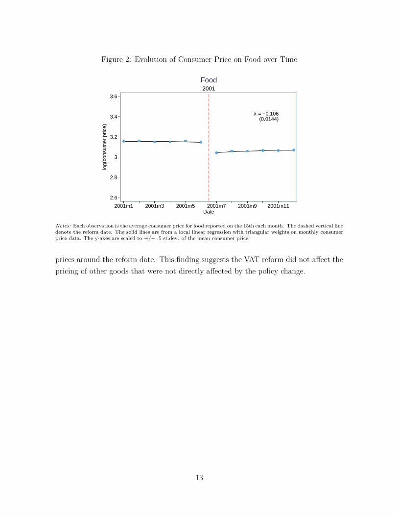
Figure 2 shows both the unrestricted and the estimated monthly means of consumerprices for food items during 2001. The estimated monthly means come from a locallinear regression with a triangular kernel applied to each side of the reform date: Whilethe regression lines better illustrate the trends in the data and the size of the jumpat the reform date, the unrestricted means indicate the underlying noise in the data.The figure shows evidence of a sharp decline in food prices at the time of the reform,suggesting that the tax is heavily shifted to consumer prices. In contrast, there is noevidence of changes in food prices prior to the VAT reform. This suggests that firmsdo not change food prices in anticipation of the VAT reform. Additionally, food pricesbarely move in the months following the reform suggesting that firms respond swiftlyto the change in VAT.
In Figure 3, we present unrestricted and estimated monthly means of consumerprices for clothing, services, household fuel, alcohol, transport and other non-durables.As in Figure 2, the scale of the y-axis is set equal to ±.5 standard deviation of themean of the respective variable. By standardizing the y-axes in this way, it becomeseasier to compare the trends in the data and the sizes of the jumps at the cut-off datesacross the graphs. In Figure 3, there is no sign of discontinuous changes in consumer
7When following the procedure of Imbens and Kalyanaraman (2012), we estimate an optimal band-width which of 1.37 months. This result motivates the choice of bandwidths in the FD and RDspecifications.
12
Figure 2: Evolution of Consumer Price on Food over Time
λ = −0.106(0.0144)
2.6
2.8
3
3.2
3.4
3.6
log(
cons
umer
pric
e)
2001m1 2001m3 2001m5 2001m7 2001m9 2001m11Date
2001Food
Notes: Each observation is the average consumer price for food reported on the 15th each month. The dashed vertical linedenote the reform date. The solid lines are from a local linear regression with triangular weights on monthly consumerprice data. The y-axes are scaled to +/− .5 st.dev. of the mean consumer price.
prices around the reform date. This finding suggests the VAT reform did not affect thepricing of other goods that were not directly affected by the policy change.
13
Figure 3: Evolution of Consumer Prices on Non-Food Items over Time
(a) Clothing
λ = −0.0192(0.0302)
4.5
5
5.5
6
log(
cons
umer
pric
e)
2001m1 2001m3 2001m5 2001m7 2001m9 2001m11Date
Clothing
(b) Services
λ = 0.0664(0.0348)
3
3.5
4
4.5
log(
cons
umer
pric
e)
2001m1 2001m3 2001m5 2001m7 2001m9 2001m11Date
Services
(c) Household Fuels
λ = −0.002(0.0388)
4.5
5
5.5
6
6.5
7
log(
cons
umer
pric
e)
2001m1 2001m3 2001m5 2001m7 2001m9 2001m11Date
HH Fuel
(d) Alcohol
λ = 0.0125(0.0162)
3
3.5
4
log(
cons
umer
pric
e)
2001m1 2001m3 2001m5 2001m7 2001m9 2001m11Date
Alcohol
(e) Transport
λ = 0.0611(0.0706)
3
3.5
4
4.5
5
log(
cons
umer
pric
e)
2001m1 2001m3 2001m5 2001m7 2001m9 2001m11Date
Transport
(f) Other Non-Durables
λ = 0.0132(0.0225)
3.5
4
4.5
5
log(
cons
umer
pric
e)
2001m1 2001m3 2001m5 2001m7 2001m9 2001m11Date
Other non−durables
Notes: Each observation is the average consumer price for the specific good reported on the 15th each month. Thedashed vertical lines denote the reform date. The solid lines are from a local linear regression with triangular weightson monthly consumer price data. The y-axes are scaled to +/− .5 st.dev. of the mean consumer price.
Our RD design assumes that consumer prices would have evolved smoothly aroundthe reform date in the absence of the policy change. This continuity condition impliesthat other observable determinants of consumer prices should have the same distribution
14
Figure 4: Evolution of Predicted Consumer Price on Food over Time
2.6
2.8
3
3.2
3.4
3.6
log(
cons
umer
pric
e)
2000m1 2000m3 2000m5 2000m7 2000m9 2000m11Date
2001Predicted food prices
Notes: Predicted food consumer prices is given by a regression of food consumer prices on oil prices (brent), euro/NOK,SEK/NOK, GDP/NOK and an import weighted exchange rate. The covariates are lagged four weeks and each observationis the average predicted consumer price for food reported on the 15th each month. The dashed vertical line denote thereform date. The solid lines are from a local linear regression with triangular weights on the predicted food consumerprices. The y-axes are scaled to +/− .5 st.dev. of the mean predicted consumer price.
just before and after the reform. For simplicity, we consider a scalar representation ofthe observable determinants, given by the predictions from a regression of food priceson a flexible set of lagged values of oil prices and exchange rates.8 The covariates arejointly predictive of food prices (F-statistic of 150). Figure 4 displays the predicted pricein each month, showing no evidence of changes in observables around the time of thereform.9 Indeed, when looking at each covariate separately, we find no evidence of anychanges around the time of the reform. Nor do the estimates of λ change appreciativelyif we add the covariates to equation 6.
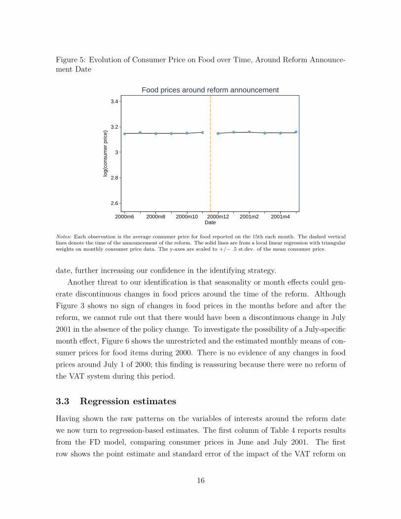
The reform was passed by Parliament (Stortinget) on December 7th, 2000. Eventhough Figure 2 already reveals that there is no discontinuous changes in food pricesfrom January 2000 and until the reform date, Figure 5 challenges the assumption ofno anticipation effects more directly. In this figure, the dashed line marks the date thereform was announced and we see no discontinuous jumps around the announcement
8We control for oil prices to proxy for energy and transportation prices. Since the price of importedfood is likely to depend on the exchange rate, we control for the import weighted exchange rate as wellas the exchange rates of Norway’s key trading partners.
9Figure 4 shows the predicted consumer price with a four week lags for the covariates. The resultsare robust to using shorter and longer lags.
15
Figure 5: Evolution of Consumer Price on Food over Time, Around Reform Announce-ment Date
2.6
2.8
3
3.2
3.4lo
g(co
nsum
er p
rice)
2000m6 2000m8 2000m10 2000m12 2001m2 2001m4Date
Food prices around reform announcement
Notes: Each observation is the average consumer price for food reported on the 15th each month. The dashed verticallines denote the time of the announcement of the reform. The solid lines are from a local linear regression with triangularweights on monthly consumer price data. The y-axes are scaled to +/− .5 st.dev. of the mean consumer price.
date, further increasing our confidence in the identifying strategy.Another threat to our identification is that seasonality or month effects could gen-
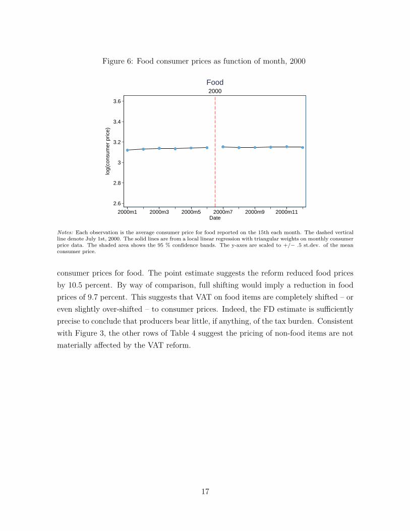
erate discontinuous changes in food prices around the time of the reform. AlthoughFigure 3 shows no sign of changes in food prices in the months before and after thereform, we cannot rule out that there would have been a discontinuous change in July2001 in the absence of the policy change. To investigate the possibility of a July-specificmonth effect, Figure 6 shows the unrestricted and the estimated monthly means of con-sumer prices for food items during 2000. There is no evidence of any changes in foodprices around July 1 of 2000; this finding is reassuring because there were no reform ofthe VAT system during this period.
3.3 Regression estimates
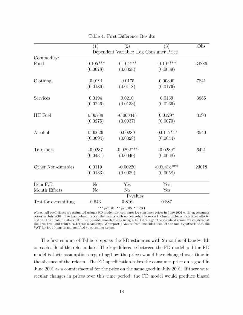
Having shown the raw patterns on the variables of interests around the reform datewe now turn to regression-based estimates. The first column of Table 4 reports resultsfrom the FD model, comparing consumer prices in June and July 2001. The firstrow shows the point estimate and standard error of the impact of the VAT reform on
16
Figure 6: Food consumer prices as function of month, 2000
2.6
2.8
3
3.2
3.4
3.6lo
g(co
nsum
er p
rice)
2000m1 2000m3 2000m5 2000m7 2000m9 2000m11Date
2000Food
Notes: Each observation is the average consumer price for food reported on the 15th each month. The dashed verticalline denote July 1st, 2000. The solid lines are from a local linear regression with triangular weights on monthly consumerprice data. The shaded area shows the 95 % confidence bands. The y-axes are scaled to +/− .5 st.dev. of the meanconsumer price.
consumer prices for food. The point estimate suggests the reform reduced food pricesby 10.5 percent. By way of comparison, full shifting would imply a reduction in foodprices of 9.7 percent. This suggests that VAT on food items are completely shifted – oreven slightly over-shifted – to consumer prices. Indeed, the FD estimate is sufficientlyprecise to conclude that producers bear little, if anything, of the tax burden. Consistentwith Figure 3, the other rows of Table 4 suggest the pricing of non-food items are notmaterially affected by the VAT reform.
Transport -0.0287 -0.0292*** -0.0289* 6421(0.0431) (0.0040) (0.0068)
Other Non-durables 0.0119 -0.00220 -0.00418*** 23018(0.0133) (0.0039) (0.0058)
Item F.E. No Yes YesMonth Effects No No Yes
P-valuesTest for overshifting 0.643 0.816 0.887
*** p<0.01, ** p<0.05, * p<0.1Notes: All coefficients are estimated using a FD model that compares log consumer prices in June 2001 with log consumerprices in July 2001. The first column report the results with no controls, the second column includes item fixed effects,and the third column also control for possible month effects using a DiD strategy. The standard errors are clustered atthe firm level and robust to heteroskedasticity. We report p-values from one-sided tests of the null hypothesis that theVAT for food items is undershifted to consumer prices.
The first column of Table 5 reports the RD estimates with 2 months of bandwidthon each side of the reform date. The key difference between the FD model and the RDmodel is their assumptions regarding how the prices would have changed over time inthe absence of the reform. The FD specification takes the consumer price on a good inJune 2001 as a counterfactual for the price on the same good in July 2001. If there weresecular changes in prices over this time period, the FD model would produce biased
18
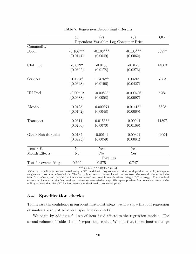
estimates of the effect of the VAT reform, because the price in June 2001 would bean inappropriate counterfactual for the price in July 2001. In this type of “smoothlycontaminated” experiment, the RD specification uses the observed trends in prices oneach side of the reform date to construct an appropriate counterfactual. As is evidentfrom the first column of Table 2, the RD estimates are very similar to the FD estimates.The point estimate reported in the first row suggests the reform reduced food pricesby 10.6 %, which supports the conclusion that consumers bear the burden of VAT onfood items. Testing for overshifting gives a p-value of 0.60, implying that we can ruleout under-shifting at conventional levels of significance. Additionally, the RD estimatesconfirm the finding of little if any spillover effects of the VAT reform to the consumerprices on non-food items.
Transport 0.0611 -0.0156** -0.00941 11897(0.0706) (0.0070) (0.0109)
Other Non-durables 0.0132 -0.00104 -0.00324 44094(0.0225) (0.0059) (0.0084)
Item F.E. No Yes YesMonth Effects No No Yes
P-valuesTest for overshifting 0.609 0.575 0.747
*** p<0.01, ** p<0.05, * p<0.1Notes: All coefficients are estimated using a RD model with log consumer prices as dependent variable, triangularweights and two months bandwidth. The first column report the results with no controls, the second column includesitem fixed effects, and the third column also control for possible month effects using a DiD strategy. The standarderrors are clustered at the firm level and robust to heteroskedasticity. We report p-values from one-sided tests of thenull hypothesis that the VAT for food items is undershifted to consumer prices.
3.4 Specification checks
To increase the confidence in our identification strategy, we now show that our regressionestimates are robust to several specification checks.
We begin by adding a full set of item fixed effects to the regression models. Thesecond column of Tables 4 and 5 report the results. We find that the estimates change
20
little when including fixed effects, suggesting the estimated reform effects are not drivenby changes in the composition of commodities over time.
Next, we estimate a difference-in-differences (DiD) specification of both the FDmodel and the RD model. The main motivation for this robustness check is thatseasonality or month effects could generate discontinuous changes in consumer prices.The DiD specification exploits the fact that there was no change in the VAT rates in2000: significant changes in the food prices in July 2000 would therefore be unrelated tothe VAT system and should instead capture month effects. A standard DiD estimate isobtained by estimating the difference in consumer prices in July versus June for the year2000, and subtract it from the FD estimate of the VAT reform. The DiD specificationof the RD model is implemented in a similar way, by separately estimating equation(6) using data from 2000 or 2001. The third column of Tables 4 and 5 report estimatesfrom the DiD specification of the FD model and the RD model, respectively. Theresults suggest that month effects do not confound the conclusions drawn about thepass-through of the VAT reform.
Lastly, we examine whether prices change in anticipation of the VAT reform. Thechange in tax rates was announced in December 2000, and it is conceivable that firmsor consumers adjust their behavior prior to the reform date. However, the graphicalevidence presented in Figure 2 showed no sign of changes in food prices outside thereform window. Further evidence against anticipation effects is provided by splittingthe set of food items into fresh and storable food. The idea is that any anticipation effectshould be stronger for storable food than for fresh food, and as a result, put downwardpressure on the estimated pass-through of the VAT reform for storable food. However,when estimating the FD and RD models separately for storable and fresh food, wefind very similar reform effects. The FD estimates of the reform effect is -0.097 (s.e.=0.0027) for storable goods, and -0.111 (s.e.=0.0039) for fresh goods. By comparison, theRD model produces estimates of the reform effect of -0.109 (s.e.=0.0047) for storablegoods and -0.098 (s.e.=0.0067) for fresh goods.
4 Distributional effects of VAT reform
The RD estimates demonstrated that the gains from the VAT reform ultimately fell onconsumers rather than producers. In this section, we investigate how the pass-throughto consumer prices affected the welfare of poor and rich households.
21
4.1 Model and estimates of demand system
Demand system. To study the welfare effects of the VAT reform, we apply the AlmostIdeal (AI) demand system first proposed by Deaton and Muellbauer (1980). In the AIdemand system, preferences belong to the Price-Independent Generalized Logarithmic(PIGLOG) class (Muellbauer, 1976) and they are defined by the expenditure function
log c (u,p) = (1− u) log a (p) + u log b (p) (7)
where u is the indirect utility and p is a vector of prices of n goods. The functionsa (p) and b (p) are specified by the following functional forms:
log a (p) = α0 +n∑i=1
αi log pi + 12
n∑i=1
n∑j=1
γ∗ij log pi log pj, (8)
andlog b (p) = log a (p) +
n∏i=1
pβii . (9)
In line with Browning and Meghir (1991) and Blundell, Pashardes, and Weber(1993), we use a two-stage budgeting framework. Preferences are characterized suchthat, in each period t, household h makes decisions on how much to consume of a set ofnon-durable commodities, conditional on household characteristics and the consump-tion level of a second group of commodities with possibly less flexible demand. Thecommodities we model directly (q) are food, clothing, services, household fuel, alcohol,transport, and other non-durable goods. The second group contains housing, somedurables, and labor-market decisions which together with household characteristics, isrepresented by z. Household utility is defined over qht for household h in period t
conditional on the set of demographics and other conditioning variables zht .The first stage of the budgeting framework is to allocate expenditures to commodi-
ties qht , denoted by mht . In the second stage of the budgeting framework, households
decide on how much to spend on food, clothing, services, household fuel, alcohol, trans-port and other non-durable goods conditional on mh
t . More specifically, inserting for(8) and (9) in (7) and applying Roy’s identity gives the second stage budget shares
whit = αhit +∑j
γij ln pjt + βhit ln[mht
a (p)
](10)
22
where whit is household h’s budget share of good i, and pjt is the price of good j
at time t. The term[mht /a (p)
]represents relative income with a (p) being a price
index. Household preferences are incorporated by allowing the constant αhit to dependon household characteristics, zhkt,
αhit = αi +∑k
αikzhkt +
∑k
δkTkt,
in which we have also added a full set of indicator variables for year and season Tkt.Both the indirect utility function and the demand functions for each good that arise
from equation (7) are linear in the log of total expenditure. Figure (1) in Section 2examined this assumption for our main commodity of interest: food items. This figureprovided a nonparametric description of the Engel curve and shows that the linearmodel seems to be a reasonable approximation for the food share curve.10
Estimation procedure. To consistently estimate (γij, βi) for every commodity i,we use the two-step estimation method of Browning and Meghir (1991) and Blundell,Pashardes, and Weber (1993). This estimation method incorporates a set of theoret-ical within-equation and cross-equation restrictions. Furthermore, it accounts for theendogeneity in mh
t in the budget share equations.The first step imposes the within-equation restrictions of adding-up and (zero-
degree) homogeneity on (10) by expressing all prices relative to the price of “other”goods together with excluding this equation from the system. Each equation is esti-mated separately, allowing for heteroscedasticity in the error terms. We use GMM toobtain unrestricted consistent estimates for each equation. Additionally, an iterativemethod is applied where one take advantage of the conditional linearity of equation (10)given a (p). That is, given a (p), the system is linear in parameters, and this suggestsa natural iterative procedure conditioning on an updates a (p) at each iteration.11
The second step imposes the cross-equation restriction of symmetry. Let φ (φ∗)denote the vector of unrestricted (restricted) parameters obtained in the step outlinedabove. The cross-equation restrictions on φ can then be expressed as
φ = Kφ∗, (11)10This is consistent with what Banks, Blundell, and Lewbel (1997) find using British household
data.11As a first approximation to a (p), we compute household-specific Stone price indices.
23
where K is a matrix of rank l − m(m − 1)/2 and l is the number of unrestrictedparameters in the demand equation system. To impose these restrictions the MCSmethod chooses an estimator φ̂∗ so as to minimize the quadratic form
φ̂∗ = arg min[φ̂−Kφ∗
]′Σ−1φ
[φ̂−Kφ∗
](12)
where φ̂ is the vector of unrestricted parameter estimates and Σφ is its estimated covari-ance matrix. The estimated covariance matrix of the symmetry constrained estimatoris given by (K′Σ−1
φ K)−1.
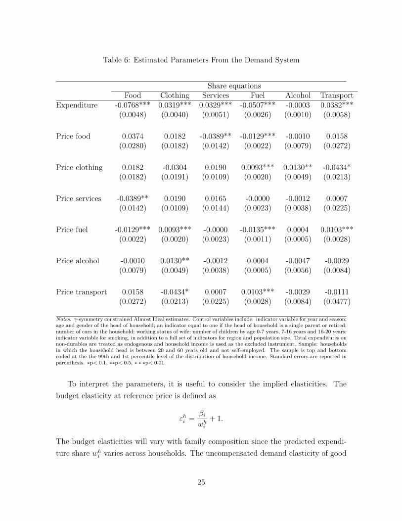
Parameter estimates and elasticities. We now turn to the estimated parametersand implied elasticities of the individual household allocations. The price and incomecoefficients that correspond to the γij and βi parameters in equation (10) are given inTable 6. From the parameter estimates we see that food and fuel are necessities, whileclothing, services and transport are luxury goods.
24
Table 6: Estimated Parameters From the Demand System
Share equationsFood Clothing Services Fuel Alcohol Transport
Notes: γ-symmetry constrained Almost Ideal estimates. Control variables include: indicator variable for year and season;age and gender of the head of household; an indicator equal to one if the head of household is a single parent or retired;number of cars in the household; working status of wife; number of children by age 0-7 years, 7-16 years and 16-20 years;indicator variable for smoking, in addition to a full set of indicators for region and population size. Total expenditures onnon-durables are treated as endogenous and household income is used as the excluded instrument. Sample: householdsin which the household head is between 20 and 60 years old and not self-employed. The sample is top and bottomcoded at the the 99th and 1st percentile level of the distribution of household income. Standard errors are reported inparenthesis. ∗p< 0.1, ∗∗p< 0.5, ∗ ∗ ∗p< 0.01.
To interpret the parameters, it is useful to consider the implied elasticities. Thebudget elasticity at reference price is defined as
εhi = βiwhi
+ 1.
The budget elasticities will vary with family composition since the predicted expendi-ture share whi varies across households. The uncompensated demand elasticity of good
25
i w.r.t. the price of good j at reference prices is given by
εuij = 1whi
[γij − βi
(αj +
N∑k=1
γjk ln pk)]− δij
where δij is the Kronecker delta. Again, we see that the elasticities vary across house-holds due to different budget shares. The compensated price elasticity is
εcij = εuij + εiwhj ,
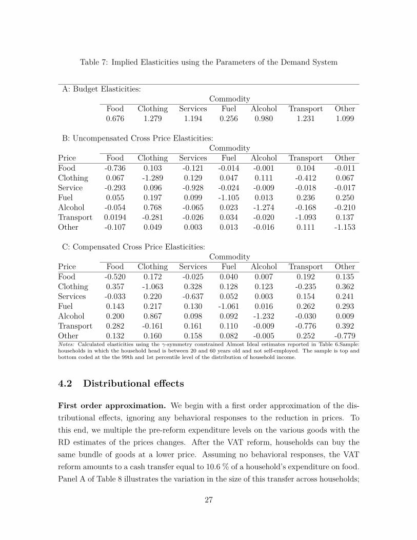
where the compensated price elasticity allows the consumers to revise their expendi-ture decision made in stage one of the budgeting framework when the price of goodj changes. The elasticities are reported in Table 7. These elasticities are calculatedfor each household individually, and then a weighted average is constructed, with theweights being equal to the household’s share of total sample expenditure of the rele-vant good. As expected, the uncompensated and compensated own price elasticitiesare negative for all goods. In terms of magnitudes, the elasticity estimates are in linewith the findings of Banks, Blundell, and Lewbel (1997)
26
Table 7: Implied Elasticities using the Parameters of the Demand System
Price Food Clothing Services Fuel Alcohol Transport OtherFood -0.520 0.172 -0.025 0.040 0.007 0.192 0.135Clothing 0.357 -1.063 0.328 0.128 0.123 -0.235 0.362Services -0.033 0.220 -0.637 0.052 0.003 0.154 0.241Fuel 0.143 0.217 0.130 -1.061 0.016 0.262 0.293Alcohol 0.200 0.867 0.098 0.092 -1.232 -0.030 0.009Transport 0.282 -0.161 0.161 0.110 -0.009 -0.776 0.392Other 0.132 0.160 0.158 0.082 -0.005 0.252 -0.779Notes: Calculated elasticities using the γ-symmetry constrained Almost Ideal estimates reported in Table 6.Sample:households in which the household head is between 20 and 60 years old and not self-employed. The sample is top andbottom coded at the the 99th and 1st percentile level of the distribution of household income.
4.2 Distributional effects
First order approximation. We begin with a first order approximation of the dis-tributional effects, ignoring any behavioral responses to the reduction in prices. Tothis end, we multiple the pre-reform expenditure levels on the various goods with theRD estimates of the prices changes. After the VAT reform, households can buy thesame bundle of goods at a lower price. Assuming no behavioral responses, the VATreform amounts to a cash transfer equal to 10.6 % of a household’s expenditure on food.Panel A of Table 8 illustrates the variation in the size of this transfer across households;
27
Table 8: Size of transfers
percentile25th 50th 75th
Panel A: First-order approximationTransfer in USD 325 490 689
Panel B: Behavioral responseCompensating variationin USD 770 1101 1455Notes: Column 1-3 show size of transfer when only allowing for direct price response to the VAT reform. Column 4-6show size of transfer allowing for both direct and indirect price responses to the VAT reform. The direct and indirectprice responses are reported in Column 2 of Table 5.
these columns report the 25th percentile, the median, and the 75th percentile of thedistribution of transfer amounts. We see that the size of the transfer is 325 USD at the25th percentile, whereas the transfer at the 75th percentile is about twice as large. Bycomparison, the median transfer is 490 USD.
Allowing for behavioral responses. There is an obvious attraction to simplyusing information on observed expenditure patterns to assess the welfare implicationsof the VAT reform. No response parameters are required, and therefore the analysis isnot subject to estimation error in own or cross-price demand elasticities. However, theVAT reform generated substantial rather than marginal changes in food prices. In suchcases, substitution effects can be non-trivial, as consumers substitute towards relativelycheaper goods. The first order approximations ignore these effects, and therefore, canbe seriously biased (see e.g. Banks, Blundell, and Lewbel, 1996).
To allow for behavioral responses, we use the parameter estimates of the AI modelto calculate the indirect utility of the households from equations (7) - (9). The transferto a given household with characteristics z is measured as the compensating variation,given by the difference in the cost functions c (p0, z, u0)− c (p1, z, u0), where the post-reform cost function is evaluated at the pre-reform indirect utility level. This welfaremeasure tells us the maximum amount of income a household is willing to pay for theVAT reform. Panel B in Table 8 illustrates the variation in the compensating variationacross households. Because a household may adjust its spending pattern in response tochanges in prices, the willingness to pay exceeds 10.6 % of the household’s expenditureon food prior to the reform. For example, the compensating variation amounts to 770USD at the 25th percentile and 1455 USD at the 75th percentile.
28
Figure 7: Household Expenditure and Compensating Variation in NOK/Year
0
500
1,000
1,500
Ave
rage
yea
rly tr
ansf
er in
US
D
0−10%
11−20%
21−30%
31−40%
41−50%
51−60%
61−70%
71−80%
81−90%
91−100%
First−order approximation Compensating variation
Notes: Notes: First-order approximation is defined as 0.894 × the pre-reform expenditure on food. Compensatingvariation is defined as the difference in the cost functionsc
(p0, z, u0
)−c(
p1, z, u0), where the post-reform cost function
is evaluated at the pre-reform indirect utility level. In calculating the post-reform cost function we allow for the directprice response to the VAT reform as reported in Column 2 of Table 5. Household income is yearly disposable householdincome. Sample: households in which the household head is between 20 and 60 years old and not self-employed. Thesample is top and bottom coded at the the 99th and 1st percentile level of the distribution of household income.
Distributional effects
We begin with a graphical depiction of the distributional effects of the VAT reform,before quantifying its impact on inequality. Figure 7 plots the magnitude of both thefirst order approximation and the compensating variation against household incomepercentiles. As rich households consume more food, the willingness to pay increaseswith total expenditure. Figure 8 complements by showing the relative size of thecompensating variation. This figure reveals that richer households are willing to pay asmaller fraction of their total expenditure for the VAT reform.
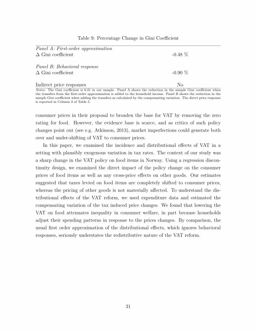
To summarize the impact of the VAT reform on inequality, we employ the muchused Gini coefficient. In 2000, the distribution of household income in our sample givesa Gini coefficient of 0.210. To assess the impact of the VAT reform, we add the sizeof the transfer to each household and compute the Gini coefficient in this simulateddistribution of household income. Panel A of Table 9 reports the change in the Ginicoefficient when the size of the transfer is computed by the first order approximation.We find that the Gini coefficient is reduced by 0.48 % when we include these transfers.
29
Figure 8: Household Expenditure and Relative Compensating Variation.
0
.01
.02
.03
.04
Rel
ativ
e ye
arly
tran
sfer
0−10%
11−20%
21−30%
31−40%
41−50%
51−60%
61−70%
71−80%
81−90%
91−100%
First−order approximation Compensating variation
Notes: First-order approximation is defined as 0.894 × the pre-reform expenditure on food. Compensating variation isdefined as the difference in the cost functionsc
(p0, z, u0
)−c(
p1, z, u0), where the post-reform cost function is evaluated
at the pre-reform indirect utility level. In calculating the post-reform cost function we allow for the direct price responseto the VAT reform as reported in Column 2 of Table 5. Household income is yearly disposable household income. Sample:households in which the household head is between 20 and 60 years old and not self-employed. The sample is top andbottom coded at the the 99th and 1st percentile level of the distribution of household income. Relative compensatingvariation is defiend as compensating variation/household income.
Panel B of Table 9 reports the change in the Gini coefficient when the size of the transferis computed by compensating variations. These transfers are substantially larger inabsolute amounts and they have a larger impact on the distribution of household incomeand we find that the Gini coefficient is reduced by 0.9 %. Put into perspective, thisreduction in the Gini coefficient corresponds to introducing a 0.9 % proportional taxon earnings and then redistributing the derived tax revenue as equal sized amounts tothe individuals (Aaberge, 1997).
5 Conclusion
Much of the controversy surrounding recent policy proposals to broaden the base forvalue added taxes (VAT) revolves around who ultimately bears the burden of thesetaxes. The typical assumption is that consumer prices fully reflect taxes, so that themain empirical question is how the tax induced price changes affect members of differentincome groups. For example, the Mirrlees Review assumes the incidence is fully on
Indirect price responses NoNotes: The Gini coefficient is 0.21 in our sample. Panel A shows the reduction in the sample Gini coefficient whenthe transfers from the first-order approximation is added to the household income. Panel B shows the reduction in thesample Gini coefficient when adding the transfers as calculated by the compensating variation. The direct price responseis reported in Column 2 of Table 5.
consumer prices in their proposal to broaden the base for VAT by removing the zerorating for food. However, the evidence base is scarce, and as critics of such policychanges point out (see e.g. Atkinson, 2013), market imperfections could generate bothover and under-shifting of VAT to consumer prices.
In this paper, we examined the incidence and distributional effects of VAT in asetting with plausibly exogenous variation in tax rates. The context of our study wasa sharp change in the VAT policy on food items in Norway. Using a regression discon-tinuity design, we examined the direct impact of the policy change on the consumerprices of food items as well as any cross-price effects on other goods. Our estimatessuggested that taxes levied on food items are completely shifted to consumer prices,whereas the pricing of other goods is not materially affected. To understand the dis-tributional effects of the VAT reform, we used expenditure data and estimated thecompensating variation of the tax induced price changes. We found that lowering theVAT on food attenuates inequality in consumer welfare, in part because householdsadjust their spending patterns in response to the prices changes. By comparison, theusual first order approximation of the distributional effects, which ignores behavioralresponses, seriously understates the redistributive nature of the VAT reform.
31
References
Aaberge, R. (1997): “Interpretation of Changes in Rank-Dependent Measures ofInequality,” Economics Letters, 55(2), 215–219.
Anderson, S. P., A. De Palma, and B. Kreider (2001): “Tax Incidence inDifferentiated Product Oligopoly,” Journal of Public Economics, 81(2), 173–192.
Atkinson, T. (2013): “The “Mirrlees Review” of UK Taxation,” Royal EconomicSociety. Newsletter, 160, 5–6.
Banks, J., R. Blundell, and A. Lewbel (1996): “Tax Reform and WelfareMeasurement: Do We Need Demand System Estimation?,” The Economic Journal,106(438), 1227–1241.
(1997): “Quadratic Engel Curves and Consumer Demand,” Review of Eco-nomics and Statistics, 79(4), 527–539.
Besley, T. J., and H. S. Rosen (1999): “Sales Taxes and Prices: An EmpiricalAnalysis,” National Tax Journal, 52, 157–178.
Blundell, R., P. Pashardes, and G. Weber (1993): “What Do We Learn AboutDemand Patterns from Micro Data,” The Amercian Economic Review, 83(3), 570–597.
Browning, M., and C. Meghir (1991): “The Effects of Male and Female LaborSupply on Commodity Demands,” Econometrica, 59(4), 925–951.
Carbonnier, C. (2007): “Who Pays Sales Taxes? Evidence from French VAT reforms,1987–1999,” Journal of Public Economics, 91, 1219–1229.
(2013): “The Incidence of Non-Linear Consumption Taxes,” Discussion paper.
Crawford, I., M. Keen, and S. Smith (2010): “Value Added Tax and Excises,”in Dimensions of Tax Design, The Mirrlees Review, ed. by J. Mirrless, S. Adam,T. Besley, R. Blundell, S. Bond, R. Chote, M. Gammie, P. Johnson, G. Myles, andJ. Poterba, chap. 4, pp. 275–422. Oxford University Press Inc., New York.
Deaton, A., and J. Muellbauer (1980): “An Almost Ideal Demand System,” TheAmerican Economic Review, 70(3), 312–326.
32
DeCicca, P., D. Kenkel, and F. Liu (2013): “Who Pays Cigarette Taxes? TheImpact of Consumer Price Search,” Review of Economics and Statistics, 95(2), 516–529.
Delipalla, S., and M. Keen (1992): “The Comparison between Ad Valorem andSpecific Taxation under Imperfect Competition,” Journal of Public Economics, 49,351–367.
Delipalla, S., and O. O’Donnell (2001): “Estimating Tax Incidence, MarketPower and Market Conduct: the European Cigarette Industry,” International Journalof Industrial Organization, 19(6), 885–908.
Doyle, J. J., and K. Samphantharak (2008): “$ 2.00 Gas! Studying the Effectsof a Gas Tax Moratorium,” Journal of Public Economics, 92(3), 869–884.
Einarsson, A. (2007): “The Retail Sector in the Nordic Countries. A ComparativeAnalysis,” Bifríst Journal of Social Science, Working Paper, 1.
Imbens, G., and K. Kalyanaraman (2012): “Optimal Bandwidth Choice for theRegression Discontinuity Estimator,” The Review of Economic Studies, 79(3), 933–959.
Kenkel, D. S. (2005): “Are Alcohol Tax Hikes Fully Passed Through to Prices?Evidence from Alaska,” American Economic Review, pp. 273–277.
Kosonen, T. (2013): “More Haircut after VAT Cut? On the Efficiency of ServiceSector Consumption Taxes,” .
Lee, D. S., and T. Lemieux (2009): “Regression Discontinuity Designs in Eco-nomics,” Discussion paper, National Bureau of Economic Research.
Marion, J., and E. Muehlegger (2011): “Fuel Tax Incidence and Supply Condi-tions,” Journal of Public Economics, 95(9), 1202–1212.
Poterba, J. M. (1996): “Retail Price Reactions to Changes in State and Local SalesTaxes,” National Tax Journal, 49, 165–176.
Seade, J. (1987): “Proftiable Cost Increases and the Shifting of Taxation: EquilibriumResponses of Markets in Oligoply,” .
33
Weyl, E., M. Fabinger, et al. (2015): “A Tractable Approach to Pass-ThroughPatterns,” in 2015 Meeting Papers, no. 747. Society for Economic Dynamics.
Young, D. J., and A. Bielińska-Kwapisz (2002): “Alcohol Taxes and BeveragePrices,” National Tax Journal, pp. 57–73.