including a new indifference rule introduction jia 73 (1947) 0285-0334

285

SOME OBSERVATIONS ON INVERSE PROBABILITY INCLUDING A NEW INDIFFERENCE RULE

BY WILFRED PERKS, F.I.A. Assistant Actuary of the Pearl Assurance Company, Ltd.

[Submitted to the Institute, 27 January 1947]

‘If the first button is buttoned wrongly, the whole vest sits askew’ —Attributed to BRUNO by HAROLD CHAPMAN BROWN

INTRODUCTION THE main object of this paper is to propound and discuss a new indifference rule for the prior probabilities in the theory of inverse probability. Being invariant in form on transformation, this new rule avoids the mathematical inconsistencies associated with the classical rule of ‘uniform distribution of ignorance’ and yields results which, particularly in certain critical extreme cases, do not appear to be unreasonable. Such a rule is, of course, a postulate and is not susceptible of proof; its object is to enable inverse probability to operate as a unified principle upon which methods may be devised of allowing a set of statistics to tell their complete and unbiased story about the parameters of the distribution law of the population from which they have been drawn, without the introduction of any knowledge beyond and extraneous to the statistics themselves. The forms appropriate for the prior probabilities in certain other circumstances are also discussed, including the important case where the unknown parameter is a probability, or proportion, for which it is desired to allow for prior bias. Before proceeding to the main purpose of the paper, however, it is convenient to provide some background to the subject. Reference is first made to certain modern writers to indicate how the problem with which inverse probability is concerned occupies a central place in the foundations of scientific method and in modern philosophy. In quoting from these writers I am not to be taken as suggesting that they necessarily support the inverse probability approach to the problem. The next section of the paper contains some brief comments on the direct statistical methods which have been devised in recent times to side-step induction and inverse probability, and this is followed by a few remarks on the various definitions of probability.

The paper is thus concerned with fundamental questions of a controversial nature, and has little, if any, immediate practical aspect, at any rate so far as applied actuarial science is concerned. No apology for this limitation is offered. On the contrary, it is suggested that the time is more than ripe for actuaries to re-examine the fundamental bases of their processes; indeed, there are not lacking signs of a general stirring of interest in these questions. Much of the spectacular progress made in other sciences (including statistics) in recent years has its origin in a reconsideration of fundamental ideas, and we find that probability theory is coming more and more to occupy a central place not only in general philosophy and scientific method but also in particular sciences such as physics and biology. Actuarial science has always been rooted in the doctrine of probability, as our charter so clearly expresses and as so many general writers on probability theory acknowledge, and it is perhaps not too fanciful to suggest that, with the common root of probability, actuarial science and these other disciplines have much in common and much to contribute to each other.

Richard Kwan

JIA 73 (1947) 0285-0334

286 Some Observations on Inverse Probability The most fundamental question of science is, of course, the problem of

induction. In the form of statistical inference, induction is the essence of actuarial science; in logic, it may be expressed as arguing from the particular to the general; in everyday life it is learning from experience. As Whitehead puts it on p. 30 of his Science and the Modern World: ‘The things directly observed are almost always only samples’ and ‘This process of reasoning from the sample to the whole species is induction. The theory of induction is the despair of philosophy-and yet all our activities are based upon it.’ On p. 48 of The Philosophy of Bertrand Russell (Vol. v of the Library of Living Philosophers), Reichenbach says: ‘I think our analysis of the problem of induction must be attached to the form of inductive inference which has always stood in the fore- ground of traditional inductive theories: the inference of induction by enumera- tion.’ Dr Sheppard, commenting on Chrystal’s unfortunate onslaught on inverse probability (T.F.A. Vol. XII, p. 26), says: ‘But he could not have been expected to foresee that, within thirty or forty years of his writing, the fundamental ideas of inverse probability would lie at the basis of a great deal of scientific work.’ In his Advanced Theory of Statistics, Kendall writes: ‘One thing, however, is clear-anyone who rejects Bayes’s postulate must put something in its place. The problem which Bayes attempted to solve is supremely important in scientific inference and it scarcely seems possible to have any scientific thought at all without some solution however intuitive and however empirical, to the problem.’

These quotations serve to show how crucial is the problem with which inverse probability is concerned. As there still seems to remain in some quarters a lingering idea that there is something ‘not quite nice’, something unsound, about the whole concept of inverse probability, it is perhaps desirable at this early stage to state, quite categorically, that, on any theory of probability, Bayes’s theorem of inverse probability is not nowadays in question (see Prof. Sir Edmund Whittaker’s paper in T.F.A. Vol. VIII, p. 163). In terms of known prior probabilities the theorem is indisputable. It is over the postulate to be adopted when the prior probabilities are not known that all the difficulties and controversy arise and, of course, it is only by the introduction of some such postulate that inverse probability can operate as a process corresponding to induction. Even Neyman, who is one of the leading exponents of, and a brilliant contributor of, new theorems and processes in the direct systems devised to side-step induction and inverse probability (see later), accepts Bayes’s theorem as ‘legitimate’ when the prior probabilities are known (Journal of the Royal Statistical Society, Vol. CV, p. 299). Unfortunately, he is so out of sympathy with what inverse probability claims to do that he classes its uses in other cases as ‘illegitimate’ and supports this classification by an example which is an outrage on the method. In this example (p. 299) of successive breeding from two Mendelian hybrids, he completely ignores the critical information which inverse probability would use, namely the relative numbers of recessives which result from the cross-breeding. When the prior probabilities are known (the ‘legitimate ’ case) these numbers add no further knowledge, but when the prior probabilities are unknown, they are of critical importance.

Fisher also recognizes inverse probability as legitimate when the prior probabilities are known, but he refers to such a case as ‘trivial’ (Statistical Methods, p. 9), and otherwise he rejects inverse probability ‘ as founded upon an error’. He is, however, willing to make certain probability statements about the unknown parameters in terms of the sample statistics, but he distinguishes such

Including a New Indifference Rule 287 statements from ordinary probability statements and from inverse probability statements by referring to them as ‘fiducial probability’ statements. It is remarkable how similar to inverse probability results Fisher’s brilliant contribu- tions to statistics often are, without departing from various direct principles.

There are, of course, many other modern writers for and against inverse probability (including particularly Keynes in his Treatise on Probability), but enough has been said by way of quotation to show the growing importance assumed by the subject in recent years. It only remains to refer to the principal modern exponent of inverse probability-Prof. Harold Jeffreys. In his book The Theory of Probability (1939), he has done much to rehabilitate the theory of inverse probability, to show its power in coping with and elucidating modern statistical problems and to provide a method corresponding to the process of ‘learning from experience’, to the process of induction. It was from a study of this work that this paper originated and the main purpose of the paper is an endeavour to remove some of the remaining difficulties in the subject which Jeffreys leaves unresolved in his book.*

DIRECT SYSTEMS It is beyond the scope of this paper to discuss at length the various direct

systems of statistical estimation and significance tests, but brief reference to similarities with and distinctions from inverse probability may be useful. On the general question of confining estimation to direct methods, it is important to appreciate that the exponents of those systems are aware that they never leave the purely conceptual sphere-the realm of pure mathematics. Neyman is at great pains (see his Lectures at the Graduate School of the U.S. Department of Agriculture) to point to the dangers of using what he calls ‘picturesque language’ in probability questions. On p. 296 of J.R.S.S. Vol. CV, he says about the set theory of probability that ‘ the probability is our conception. . . but these conceptions imitate some real observable phenomena’, and on p. 294 he says that ‘the method of approach of von Mises has the advantage of frankly and directly attacking the problem of a model of the phenomena of the outside world’. He adds that as far as he can see, ‘from the point of view of applications both theories are equivalent ‘. There seems to be something suggestive about his use of the epithet ‘subjective’ for Jeffreys’s theory of probability-almost that his own approach is ‘objective’. He insists (p. 323) that he uses the word ‘probability’ only in one connexion—probability of an object A having a property B-and yet I cannot believe that he identifies what is purely conceptual with the purely objective. It may be noted that in a particular problem (p. 323) he uses the label ‘objects’ for ‘random selections’. He refers to his own theory (based on the mathematical theory of sets-see later) as ‘classical’. Can there be here an appropriate analogy with pre-Einstein physics, a return to crude materialism— naïve realism, as Jeffreys put it ? The answer that would no doubt be given is that the application of the mathematical model to the ‘real’ world must be subject to the test of experience. But without prescribing a test external to the model we are in a conceptual circle. If the test is in terms of conceptual operations, such as infinite random selections, the circle is complete. If the test is in terms of physical operations it is, I think, clear that it never can be powerful enough to determine the issue at its fundamental level which remains obscured by the inevitable sampling uncertainty. Fisher (p. I of The Design of

* See Addendum on p. 311.

288 Some Observations on Inverse Probability Experiments) appears to accept the difficulty frankly by confining the science of statistics to a branch of pure mathematics, leaving the practical problem of scientific inference as a ‘ question of the right use of human reasoning powers’ on which the mathematical statistician, ‘ as such, speaks with no special authority’. This attitude is the antithesis of Laplace’s attitude, which is summed up in the well-known quotation: ‘ La théorie des probabilités n’est que le bon sens réduit au calcul.’ The actuary, as a practising statistician, knows that Fisher’s escape is not possible-he is forced by the nature of his work to make inferences for practical purposes. Whitehead puts the position well in his Science and the Modern World (p. 70) : ‘ The great characteristic of the mathematical mind is its capacity for dealing with abstractions; and for eliciting from them clear-cut demonstrative trains, entirely satisfactory so long as it is those abstractions which you want to think about.’ If we read this in conjunction with what he says about materialism–‘ The doctrine which I am maintaining is that the whole concept of materialism only applies to very abstract entities, the products of logical discernment –and with what he says about induction–‘ Induction pre- supposes metaphysics. In other words it rests upon an antecedent rationalism’ –we have, I suggest, the philosophy of deductive estimation in a nutshell.

It is, I think, clear that all the direct methods involve at some stage the introduction of an arbitrary principle of some kind. It is not suggested that these principles may not be highly plausible-they often are; that may be why the results to which they lead are closely similar to the results of inverse probability applied to the same problems. What is important is that arbitrary principles are introduced and that some of them have an affinity with the indifference rule in inverse probability. The simplest case is the principle of maximum likelihood, although Fisher appears to deny any logical affinity in this case. However, when the possible values of the unknown parameter are discrete, maximum likelihood and maximum posterior probability (using Bayes’s indifference rule) give ‘the same answer and are equivalent’ (Kendall, The Advanced Theory of Statistics, Vol. I, p. 178). When the permissible values of the unknown parameter are continuous, differences can arise, and indeed inconsistencies can arise, within inverse probability, if Bayes’s postulate is applied to different functions of the unknown parameter (see Kendall, p. 179). Kendall explains how this arises, but he does not overcome the embarrassment of choice; he is, of course, discussing the matter from the point of view of maximum likelihood. Later in this paper, a general solution of this difficulty is put forward.

I need say nothing about such notions as unbiased statistics, efficient statistics and the like; the arbitrary principles involved are obvious. On the other hand, the introduction of an arbitrary principle (and its nature) in the use of ‘ Student’s’ rule and of confidence intervals generally is not so clear. The plain object of ‘ Student’s’ distribution and confidence intervals is to provide methods by which the statistics can be allowed to speak for themselves and to exclude extraneous information, an object which they have in common with the indifference rule in inverse probability. In his paper entitled Mathematics and Agronomy (see Collected Papers) ‘ Student’ states that ‘the tables are calculated to give the odds correctly if all the available information is contained in the sample’. He adds characteristically that ‘in fact, tables can only be an aid to, and not a substitute for, common sense’ -an outlook of special appeal to any actuary. Jeffreys (p. 310) points out the significance of the words ‘unique sample’ in the heading of ‘ Student’s’ tables and goes on to trace the point in ‘ Student’s ’ and Fisher’s demonstrations where he suggests that the assumption

Including a New Indifference Rule 289

of an indifference rule is implicit. The argument is difficult, but this, at any rate, is clear, namely, that Jeffreys, by using his special rule for the prior probabilities of a standard deviation (see later), produces the t-distribution by inverse probability principles.

For confidence intervals generally there is a further difficulty. The principle of confidence intervals may be stated as follows. If in a long series of sampling experiments a statement is made that the universe parameter is contained within a pair of limits, defined by certain specified rules in terms of the statistics of each sample, the statement will, in the long run (presumably in the probability sense), prove to be right in about k %. of the cases, where k can be fixed at will ‘and the appropriate rules are deduced accordingly. This k % statement is referred to as a ‘confidence statement’ and the word ‘probability’ is avoided. From the standpoint of the frequency theory of probability, however, it would seem that k does represent a probability provided that we take our stand before we have made a particular sample (i.e. before we know the result of the sample). I find it difficult to escape the conclusion that we have here a peculiar form of prior probability about a statement expressed in terms of the actual statistics and the unknown parameter. The whole theory of confidence intervals is a brilliant piece of deduction, but the difficulty to me is that the confidence statement has still to be made when we know the result of the sample, notwithstanding that, except in certain special cases, this additional knowledge may modify the probability of the correctness of the statement. The amount of this modification may be quite small in the usual cases of application, and it may be that it would be argued that it is only on the basis of inverse probability as derived from a theory of probability such as that of Jeffreys that the distinction has meaning. On the other hand, it may not be unreasonable to suggest that it is precisely because the confidence interval results differ so little (and not at all in certain cases) from inverse probability results that they do in fact inspire confidence.

It is clear that the direct schools present for choice an embarrassing array of methods of estimation; and some of them involve confusions and differences when estimates of more than one parameter at a time are required. They approach perilously near to inverse probability in places and yet remain purely deductive and conceptual. A satisfactory basis for inverse probability-a resolute attack on any remaining doubtful points-would avoid these difficulties and would include the problem of inductive inference as an integral part of statistical method instead of leaving it as an unsystematized process beyond the science of statistics.

DEFINITIONS OF PROBABILITY Laplace’s definition of probability was to the effect that, if an event can happen

in m ways and fail in n ways and all (m + n) ways are mutually exclusive and equally likely, the probability of the happening of the event is m/(m + n). The common objections to this definition are (I) that the inclusion of the words ‘equally likely’ makes the definition circular, and (2) that it is difficult to bring within the definition such cases as loaded dice. There may be added a third: that it confines probabilities to the rational numbers.

The neo-classical school (the principal exponents in English are Cramer, Neyman and Wilks) overcome the second and third of these objections by an appeal to the mathematical theory of sets and claim to avoid the first objection– at any rate they exclude the words ‘equally likely’ from their definition in terms of sets. It seems to me that the ratio of the measures of two sets, however defined, remains a ratio until the notion of selection at random is introduced,

290 Some Observations on Inverse Probability and this notion would appear to include the notion of ‘equally likely’. This is, I think, what Jeffreys means when he says that this school implicitly introduces the notion of ‘ reasonable degree of belief’ before the ink in which the definition is written is dry. He also points out that if x is a measure of a set so is f(x), where f (x) is a monotonic function of x, so that the definition without ‘equally likely ’ lacks precision.

Now I want to suggest that the objection that the words ‘equally likely’ involve circularity is itself an invalid objection. For this purpose I quote from Hans Reichenbach (p. 29, loc. cit.) as follows: ‘ Russell’s definition of number is based on the discovery anticipated in Cantor’s theory of sets, that the notion of “ equal number” is prior to that of number. Using Cantor’s concept of similarity of classes, Russell defines two classes as having the same number if it is possible to establish a one-to-one co-ordination between the elements of these classes.’

Without pursuing here the steps by which the integers are developed out of this notion, it seems clear that any identification of a ratio of measures of sets with probability involves the identification of probability with number and hence of equal probability with equal number, so that ‘equally likely’ is a notion prior to probability. Thus the incorporation of ‘equally likely’ in the neo-classical definition would not involve circularity, but would treat ‘equally likely’ as a primitive notion, as in effect Jeffreys maintains. Going back to the Laplace definition we see that the statement that ‘an event can happen in m ways and fail in n ways all of which are mutually exclusive and equally likely’ is a meaningful statement about these (m + n) ways, although it actually tells us nothing about the strength of the probability until we add that there are no other ways, or, to express it in a better way, that one of them must happen. As this statement about the (m + n) ways is meaningful without saying anything about the measure of probability until a further statement is added, it is suggested that with this addition the definition is not circular. This addition has, of course, always been assumed to be implied in the definition.

Turning now to the frequency definitions there seem to me to be two fatal objections. First, they confine probabilities to the rational numbers, and yet their advocates pass over to the irrational numbers in continuous probability problems without justifying this step. The second objection turns on the assumption that the relative frequency tends to a limit as the number of trials tends to infinity. Jeffreys points out that this process to a limit is not the ordinary mathematical limiting process, and that for the expression of any such limit to be sound it must be expressed in probability terms and we have a circular definition with a vengeance ! (See also Elements of Probability, by Levy and Roth, p. 142.)

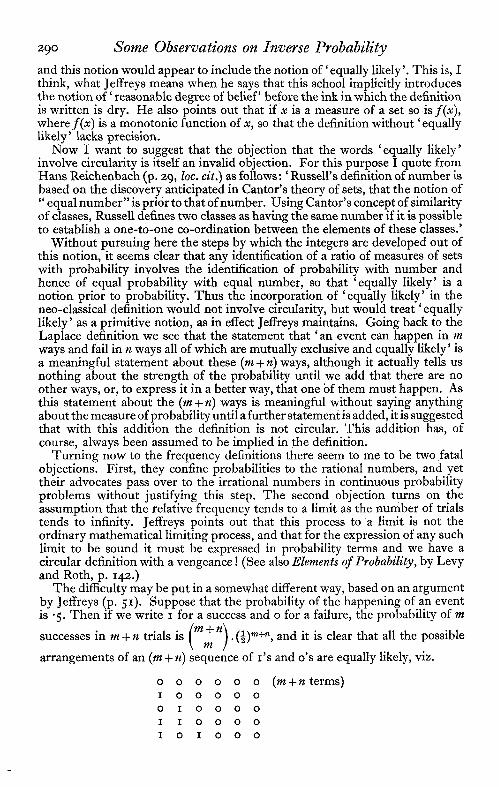
The difficulty may be put in a somewhat different way, based on an argument by Jeffreys (p. 51). Suppose that the probability of the happening of an event is .5. Then if we write I for a success and o for a failure, the probability of m

successes in m + n trials is , and it is clear that all the possible

arrangements of an (m + n) sequence of 1'S and 0’s are equally likely, viz.

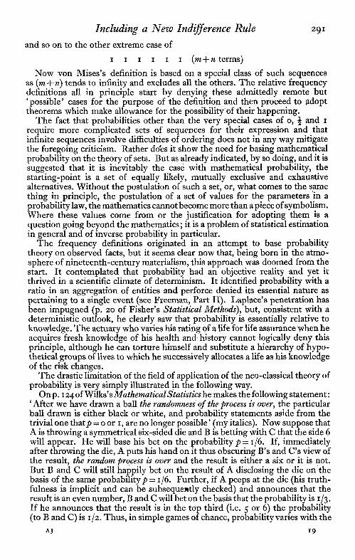
0 0 0 0 0 0 ( m+ n terms) 1 0 0 0 0 0 0 1 0 0 0 01 1 0 0 0 010 1 0 0 0

Including a New Indifference Rule and so on to the other extreme case of

291

1 1 1 1 1 1 (m + n terms) Now von Mises’s definition is based on a special class of such sequences

as (m+n) tends to infinity and excludes all the others. The relative frequency definitions all in principle start by denying these admittedly remote but ‘possible’ cases for the purpose of the definition and then proceed to adopt theorems which make allowance for the possibility of their happening.

The fact that probabilities other than the very special cases of o, ½ and 1 require more complicated sets of sequences for their expression and that infinite sequences involve difficulties of ordering does not in any way mitigate the foregoing criticism. Rather does it show the need for basing mathematical probability on the theory of sets. But as already indicated, by so doing, and it is suggested that it is inevitably the case with mathematical probability, the starting-point is a set of equally likely, mutually exclusive and exhaustive alternatives. Without the postulation of such a set, or, what comes to the same thing in principle, the postulation of a set of values for the parameters in a probability law, the mathematics cannot become more than a piece of symbolism. Where these values come from or the justification for adopting them is a question going beyond the mathematics; it is a problem of statistical estimation in general and of inverse probability in particular.

The frequency definitions originated in an attempt to base probability theory on observed facts, but it seems clear now that, being born in the atmo- sphere of nineteenth-century materialism, this approach was doomed from the start. It contemplated that probability had an objective reality and yet it thrived in a scientific climate of determinism. It identified probability with a ratio in an aggregation of entities and perforce denied its essential nature as pertaining to a single event (see Freeman, Part 11). Laplace’s penetration has been impugned (p. 20 of Fisher’s Statistical Methods), but, consistent with a deterministic outlook, he clearly saw that probability is essentially relative to knowledge. The actuary who varies his rating of a life for life assurance when he acquires fresh knowledge of his health and history cannot logically deny this principle, although he can torture himself and substitute a hierarchy of hypothetical groups of lives to which he successively allocates a life as his knowledge of the risk changes.

The drastic limitation of the field of application of the neo-classical theory of probability is very simply illustrated in the following way.

Onp. 124 of Wilks’s MathematicalStatistics he makes the following statement: ‘After we have drawn a ball the randomness of the process is over, the particular ball drawn is either black or white, and probability statements aside from the trivial one that p =0 or 1, are no longer possible’ (my italics). Now suppose that A is throwing a symmetrical six-sided die and B is betting with C that the side 6 will appear. He will base his bet on the probability p = 1/6 If, immediately after throwing the die, A puts his hand on it thus obscuring B’s and C’s view of the result, the random process is over and the result is either a six or it is not. But B and C will still happily bet on the result of A disclosing the die on the basis of the same probability p= 1/6 Further, if A peeps at the die (his truth- fulness is implicit and can be subsequently checked) and announces that the result is an even number, B and C will bet on the basis that the probability is . If he announces that the result is in the top third (i.e. 5 or 6) the probability (to B and C) is . Thus, in simple games of chance, probability varies with the

AJ 19

292 Some Observations on Inverse Probability degree of knowledge of the result after the random process is over, and no theory is adequate which fails to take account of the effect of such knowledge on the probability.

It is, I think, clear that the foregoing examples of the obscured die, with partial disclosure of the result, can be embraced in the set theory or in a relative frequency theory, but to permit this would be to renounce the claim that the theory is ‘objective’, unless the word ‘objective’ is confined to ‘conceptual objects’ or ‘objects of thought’. Probability regarded solely as a property of a common-sense object and an undefined random process (see p. 2 of Wilks’s Mathematical Statistics) not only drastically confines the scope of the theory but also requires the acceptance of a naive metaphysic. To permit the incursion of the knowledge of the observer as affecting the probability is to descend the slippery slope and there is no stopping point short of the limiting position of complete absence of knowledge involving the need for indifference rules.

It is clearly not inconsistent with the modern principle of indeterminism to postulate an objective chance without asserting the possibility of ever being able to measure it with complete precision, and probability then becomes a problem of estimation relative to a body of knowledge. In so far as this knowledge is confined to statistical knowledge a precise process of inverse probability should be possible of attainment. Without some such approach probability cannot come into its rightful focus as the centre of a calculus of observations and as the essential basis for scientific method. To confine it to pure mathematics is to sterilize it and to deny its essential function. The following further quotations from Reichenbach and Russell seem to me to express clearly what is at stake:

‘Russell has repeatedly emphasized the need for inductive methods and recognized the peculiar difficulties of such methods. He thus makes it clear that he does not belong to the category of logicians who claim that the cognitive process can be completely interpreted in terms of deductive operations, and who deny the existence of an inductive logic. It is indeed hardly understandable how such utterances can be made, in view of the fact that knowledge includes predictions, and that no deductive bridge can lead from past experiences to future observations. A logic which does not include an analysis of inductive inference will always remain incomplete.’ (Reichenbach, p. 47, loc. cit.)

‘But it seems clear that whatever is not experienced must, if known, be known by inference. I find that the fear of solipsism has prevented philosophers from facing this problem, and that either the necessary principles of inference have been left vague, or else the distinction between what is known by experience and what is known by inference has been denied. If I ever have the leisure to under- take another serious investigation of a philosophic problem, I shall attempt to analyse the inferences from experience to the world of physics assuming them capable of validity, and seeking to discover what principles of inference, if true, would make them valid. Whether these principles, when discovered, are accepted as true, is a matter of temperament; what should not be a matter of temperament should be the proof that acceptance of them is necessary if solipsism is to be rejected.’ (Russell, p. 16, loc. cit.)

Even if space permitted, I should not wish to attempt! to summarize Jeffreys’s exposition of his theory of probability or his criticism of the other theories. His. work calls for first-hand study. I will confine myself to the quotation of his first axiom: ‘Given p, 4 is either more or less probable than r, or both are equally probable; and no two of these alternatives can be true.’ Thus ‘equal probability’ is taken as a primitive notion.


I conclude this section of the paper by expressing the view that no theory of probability can escape an antecedent philosophy and metaphysic, and that, as, in the theory of relativity, objectivity and subjectivity are subsumed in a theory about observations, about the relation between the observer and the ‘object’ of observation, so probability theory must be a theory about observations rather than about objects or about pure concepts if it is to correspond adequately with scientific inference.

THE INVERSE PROBABILITY THEOREMThe general inverse probability theorem is expressed by Jeffreys in the

following form:Posterior probability Prior probability x Likelihood.

It is assumed that a sample has been obtained at random from a population distributed according to a probability law. The form of this probability law is assumed to be known, but the values of the parameters in the law are assumed to be unknown. This is the essential position in estimation problems and is common to the deductive methods and inverse probability. The assumption of the probability law rests on a question of significance, and, as Jeffreys puts it, every estimation problem assumes that a prior significance problem has been solved. This paper does not pursue the application of inverse probability to significance testing.

Assuming a particular set of values of the parameters, the likelihood expresses the probability of the sample arising on the basis of the probability law with these values of the parameters. The prior probability expresses the probability that these parameters have these particular values before the result of the sample is known. The posterior probability expresses the probability that the parameters have these particular values after the result of the sample is known. The sign is used to indicate that a constant multiplier may be necessary to ensure that the sum of the posterior probabilities for all possible sets of values of the parameters is equal to unity.

Thus, if we know the law and also the values of the prior probabilities the theorem is clearly based on the product rule for compound probabilities and there is nowadays no dispute on its validity in these conditions (see Whittaker’s paper On some disputed questions in probability, T.F.A. Vol. VIII, p. 163).

THE BAYES-LAPLACE POSTULATEThe difficulties and controversy arise in the vital cases where the prior

probabilities are not known and where, if it is desired to use the theorem, an assumption must be made regarding the values of these prior probabilities. In particular, the critical problem turns on the question of whether formal mathematical expression can properly be given (and, if so, what mathematical form should be assigned) to these prior probabilities when, before the sample is taken, we are in a state of complete ignorance, or when it is appropriate for us to assume that we are in complete ignorance, about the values of the parameters, subject only to any necessary limitations implicit in the underlying probability law itself (such as that the parameter must lie between o and I or between o and ). It has been argued by some that complete ignorance cannot be expressed in mathematical terms, a view which has been summed up in the tag ex nihilo nihil.

19-2

294 Some Observations on Inverse Probability As Jeffreys points out, such an attitude forbids any theory to start at all, and I would add that it denies the possibility of ever devising a process by which a set of statistics can be allowed to speak for themselves, without the introduction of external information. For my part, I reject this view entirely. I also reject the idea that we can properly obtain any guidance on the point from experience; for example, that we can in the binomial case obtain any guidance from the distribution of observed statistical ratios on the lines suggested by Karl Pearson and criticized by Jeffreys.

To meet the difficulty Bayes, with a great deal of doubt, suggested (and Laplace, apparently with little sign of doubt, adopted) the ‘indifference rule’ that each set of values of the parameters should be given equal prior probabilities.

Before proceeding to discuss the difficulties involved in this rule and my proposal for overcoming them, it is convenient to set out the well-known results in the classic case of the binomial law. I shall confine attention to the case where the parameter in the binomial law can take any value in the continuum from o to I. Indeed, this paper will be confined to the problem of continuous parameters which provide the basis for most of the difficulties in the subject.

THE BINOMIAL LAW Let us assume that samples are drawn from a population and that the proba-

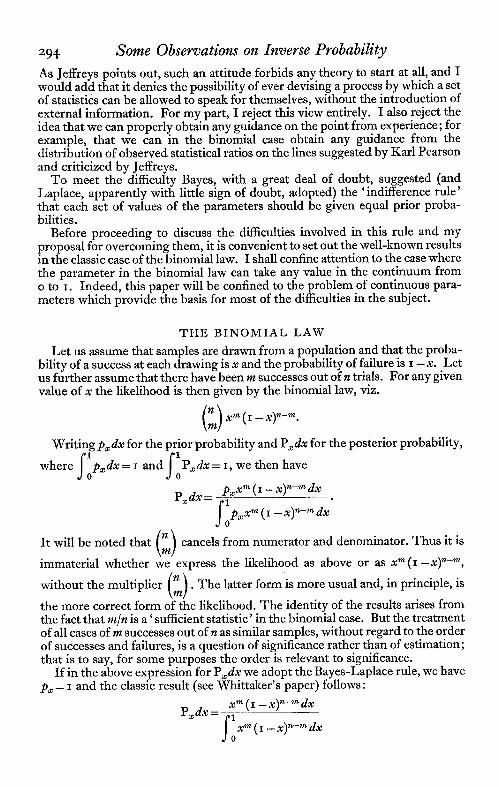
bility of a success at each drawing is x and the probability of failure is 1—x. Let us further assume that there have been m successes out of n trials. For any given value of x the likelihood is then given by the binomial law, viz.

Writing px for the prior probability and Pxdx for the posterior probability,

where and

It will be noted that cancels from numerator and denominator. Thus it is

immaterial whether we express the likelihood as above or as xm (1– x)n–m,

without the multiplier . The latter form is more usual and, in principle, is

the more correct form of the likelihood. The identity of the results arises from the fact that m/n is a ‘sufficient statistic’ in the binomial case. But the treatment of all cases of m successes out of n as similar samples, without regard to the order of successes and failures, is a question of significance rather than of estimation; that is to say, for some purposes the order is relevant to significance.

If in the above expression for Pxdx we adopt the Bayes-Laplace rule, we have px = 1 and the classic result (see Whittaker’s paper) follows :

we then have


The mean value of the Px distribution is (m + 1)/(n + 2). This represents the probability of the next trial being a success since the total probability of a

success next time is If m = n the probability of a success next time is

(n+ 1)/(n+2), h f t e amous rule of succession. If m = n/2 this probability is .5 and if m = o, it is 1/(n + 2).

The mode of the Px distribution gives the maximum posterior probability, namely m/n, and this is, of course, identical with the maximum likelihood.

There is one further result needed in the sequel and that is the probability that, after n successes inn trials, the next (n + I) trials will all be successes. This result, due to Karl Pearson, is obtained from

since m = n and n - m = o, and the probability works out at .5.

THE DIFFICULTIES ARISING FROM THE BAYES-LAPLACE RULE

If all parameters had a possible range of - to co, and before sampling wehad no reason to prefer one value rather than any other, the Bayes Laplace rule might have withstood much of the criticism to which it has been subjected and inverse probability might have contributed much more to the theory of statistics than it has. At any rate, in cases of unlimited possible variation (such as a mean in a normal universe) the Bayes-Laplace indifference rule does not seem to have led to much difficulty. The difficulties arise in the cases where the range of possible variation is limited either at one end (e.g. in the case of a standard deviation or variance which cannot be less than zero) or at both ends (e.g. in the case of a proportion or a probability for which the possible range is o to I). These difficulties may be grouped under two headings :

(I) The rule can lead to unreasonable, or unacceptable, results ; (2) The rule can lead to inconsistent results. At one time, the rule of succession was regarded as a logical justification for

induction, for scientific inference. But Pearson’s result of .5 for the probability that the next (n + I) trials will be successes, after n successes in n trials, is clearly too low and unacceptable as a representation of the scientific process of experimentation to test a proposed scientific law. As Jeffreys says (p. 102), the result does not correspond with anybody’s way of thinking. The rule of succession itself is hard to accept. It assigns a probability to the next trial which implies the assumption that the actual run observed is an average run and that we are always at the end of an average run. It would, one would think, be more reasonable to assume that we were in the middle of an average run. Clearly a higher value for both probabilities is necessary if they are to accord with reasonable belief. Having in mind the limitation of variation of the probability parameter to the range o to I, Jeffreys considers the possibility of transforming to another variable with an infinite range both ends and of applying the Bayes-Laplace rule to this other variable. He illustrates this by the transformation

y=log{x/(1 -x)}. This yields the form pydy = dy = dx/x ( I - x) =pxdx for the prior probabilities and the resulting probability for the next trial, after m successes in n trials, is

296 Some Observations on Inverse Probability m/n, or certainty when m=n and impossibility when m=o. As Jeffreys remarks, these results go too far in the other direction, and we still have unreasonable results for the extreme cases. Jeffreys does not pursue this particular aspect of the subject further.

The other group of difficulties is even more serious. It arises from the fact that if we transform the variable non-linearly and apply the Bayes-Laplace rule to the transformed variable we necessarily obtain results which are discrepant with those obtained by applying the rule to the original variable. This would not be serious if we could be sure that a particular variable was of unique relevance to our problem, that in each problem there was, so to speak, some known absolute metric. Einstein has taught us to beware of such assumptions, but it does not need any excursion into relativity to see that the choice between say a variance and a standard deviation, as the form of expression of an unknown parameter, is quite arbitrary. The separate application of the Bayes-Laplace rule to these two parameters obviously yields discrepant results for the posterior probabilities. Jeffreys successfully overcomes the difficulty in this case by means of an ad hoc rule for the prior probabilities whenever the possible range of the parameter is from o to . This rule is pxdx=dx/x, so that if we write y = xn we have dy/y dx/x. By this rule it is immaterial whether we use the variance or the standard deviation as our parameter. The rule is not, of course, invariant for other forms of transformation and is quite independent of the rules for parameters which are either limited at both ends or unlimited at both ends.

THE NEW INDIFFERENCE RULEThe limited invariance of this rule of Jeffreys for parameters with a range

limited at one end, coupled with the brilliant results achieved by him, including the derivation of important statistical distributions (e.g. the t-distribution and the x-distribution) and the elucidation of important modern statistical notions (e.g. the notion of ‘sufficient statistics’) by inverse probability processes, suggests that there is much more in this matter than a mere lucky ad hoc rule. Clearly what is wanted is a unified rule which embraces this ad hoc rule and which can be applied to all kinds of parameters and is invariant to all forms of transformation. Such a rule would comply with the general process of minimiza- tion of postulates, i.e. it would satisfy the simplicity postulate (Ockham’s razor) which Jeffreys rightly stresses as of fundamental importance to science. The provision of such a rule would then fall to be tested by the results to which it leads. Like any other postulate it is not a matter for proof; its acceptability turns on its fruitfulness, on the reasonableness and consistency of the results to which it leads.

Bearing in mind that the prior probabilities are assigned to particular small intervals in the range of possible variation of the parameters and not to points or particular values of the parameters, the rather obvious need is to assign equal probabilities not to equal arbitrary intervals but to equal ‘standardized’intervals. The more or less intuitive approach which led to this conception is indicated in the next section by reference to the notion of confidence intervals. In this section the new rule is stated and some of its properties are examined. The new rule may be stated as follows:

Including a New Indifference Rule 297 where x is a parameter in a probability law of any form, which can take any value in a given continuum, whether unlimited, limited at one end or limited at both ends. x is the large sample standard error of X. Where x is the mean of a binomial distribution, or a mean or a standard deviation of a normal distribution, or, more generally, where x is a parameter for which there is a ‘sufficient statistic’ (i.e. a statistic which contains the whole of the information in a sample relevant to the parameter), then, provided that the parameter is a function of the universe distribution of the same form as the statistic is of the sample distribution, x is the large sample standard error of that statistic. In cases where there is no

‘sufficient statistic’ the meaning of x is somewhat vague, but it seems reasonable to define it as the large sample standard error of whatever ‘consistent’ statistic is used as relevant to the parameter. If we transform the rule dx/ x, by y = f(x) we then have

That this rule is invariant on transformation (i.e. that it retains its form on transformation) is clear from the differential equation which connects the large sample standard error of a function of a statistic with the standard error of the statistic itself (e.g. see Kendall, p. 208) and can be shown in the following simple way.

Suppose that we have a set of large sample statistics xi (e.g. a set of means or standard deviations) measured from the universe parameter and that y = f(xi) is a function of the statistic xi which is capable of expansion by Taylor’s theorem, so that

Then in the limit for large samples

and

Hence

In the case of a normal universe, it is known that sample means and standard deviations are independent. Thus writing x for the mean as a parameter with an unlimited range of possible variation, x is independent of x and the new rule reduces to the Bayes-Laplace rule pxdx dx.

The standard error of a standard deviation is

298 Some Observations on Inverse Probability For a normal universe this reduces to / (2n) and so the new rule, in this case, reduces to Jeffreys’s ad hoc rule for parameters limited at one end viz.,

It should be noted, therefore, that Jeffreys’s rule applies only when the standard error reduces in this way and Jeffreys’s suggestion that dx/x should be used for parameters with a range of o to co is not universally appropriate. Fortunately, his important results for normal universes and certain other cases are not affected.

In the case of a probability parameter where the law of variation is the binomial, the standard error is x½ (1 - x)½/ n and the new rule gives

or

This is a U-shaped distribution, with a finite area, a mean of .5 (complying with the requirement that the probabilities of success or failure at the first trial should be equal) and infinite ordinates at the end-points x = o and x = 1 .*

It is of interest to note that it is a special case of the form xr (1 - x)s suggested by Hardy (in the correspondence reprinted from the Insurance Record (1889) in the same volume of T.F.A. as Whittaker’s paper) as suitable for expressing a degree of prior knowledge, because of its cocked-hat shape when r and s are positive and because of the facility with which it combines with the likelihood function. In the discussion on Whittaker’s paper Lidstone refers to the possibility of using negative values of r and s to provide U-shaped curves for cases where high probabilities near the extremes would be appropriate. Neither of them, however, contemplated putting r = s = -½ to obtain an indifference rule in place of the Bayes-Laplace rule, which of course results from r = s = o.

Probability theory has for so long been constructed on the basis of confining probabilities to the continuum o to 1, with o representing impossibility and 1 representing certainty, that we are inclined to regard this as somehow necessary instead of as a quite arbitrary procedure imposed by the mind in order to facilitate the working in the mathematical superstructure. Jeffreys illuminates this point in his own approach on an axiomatic basis. He shows that the commencing value o is a necessary consequence of his axioms and of the adoption of the addition rule as a convention; but the adoption of 1 as the other limit is also conventional and he shows that for some purposes it may not even be the most convenient convention.

Since the distinction between ‘success’ and ‘failure’ is a matter of nomen- clature (q and p entering symmetrically into probability expressions) and since for ‘impossibility’ we can speak of ‘certainty of failure’, a limit at either end is clearly a matter of convenience rather than of necessity. An obvious transformation to a continuum unlimited at one end would be to use as a scale of probability the odds against an event, i.e. if x is the usual probability, the reciprocal of the

* In connexion with the problem of a finite universe in which the only possible values of x are o/N, 1/N, z/N, . . . , N/N, Jeffreys gives cogent reasons for special weight being given to the extreme values o/N and N/N and suggests certain arbitrary rules for this purpose. It is interesting to note that if we use 1/N x½ (1 -x)½ for the prior probabilities of the intermediate values of x and split the balance of the total probability equally between the two extreme values of x (o/N and N/N), the requirements of the discrete case as indicated by Jeffreys (p. 109) are met and in the limit the new rule for the continuous case is reached.

Including a New Indifference Rule 299 odds against the event is x/(1 – x) which has a range of 0 to (cf. the American actuarial symbol kx = qx/px). Enough has been said perhaps to indicate that the application of the Bayes-Laplace rule to probability intervals in the continuum 0 to 1 is a quite arbitrary procedure and that the new rule has the important merit of avoiding the necessity of an arbitrary choice of continuum in this most important case in which difficulties have arisen out of the Bayes-Laplace postulate.

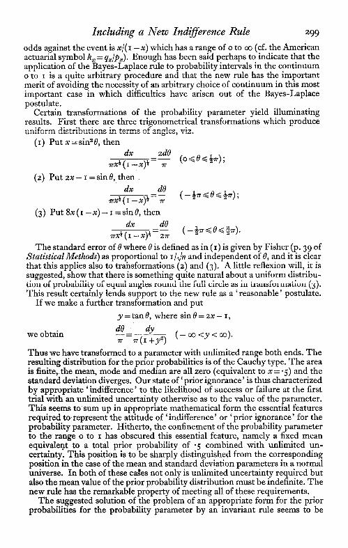
Certain transformations of the probability parameter yield illuminating results. First there are three trigonometrical transformations which produce uniform distributions in terms of angles, viz.

(1) Put x = sin2 , then

(2) Put 2x- 1 =sin , then

(3) Put 8x(1-x) - 1 = sin , then

The standard error of where is defined as in (1) is given by Fisher (p. 39 of Statistical Methods) as proportional to 1/ n and independent of , and it is clear that this applies also to transformations (2) and (3). A little reflexion will, it is suggested, show that there is something quite natural about a uniform distribution of probability of equal angles round the full circle as in transformation (3). This result certainly lends support to the new rule as a ‘reasonable’ postulate.

If we make a further transformation and put y=tan , where sin =zx-1,

we obtain

Thus we have transformed to a parameter with unlimited range both ends. The resulting distribution for the prior probabilities is of the Cauchy type. The area is finite, the mean, mode and median are all zero (equivalent to x = .5) and the standard deviation diverges. Our state of ‘prior ignorance’ is thus characterized by appropriate ‘indifference’ to the likelihood of success or failure at the first trial with an unlimited uncertainty otherwise as to the value of the parameter. This seems to sum up in appropriate mathematical form the essential features required to represent the attitude of ‘indifference’ or ‘prior ignorance’ for the probability parameter. Hitherto, the confinement of the probability parameter to the range o to 1 has obscured this essential feature, namely a fixed mean equivalent to a total prior probability of .5 combined with unlimited uncertainty. This position is to be sharply distinguished from the corresponding position in the case of the mean and standard deviation parameters in a normal universe. In both of these cases not only is unlimited uncertainty required but also the mean value of the prior probability distribution must be indefinite. The new rule has the remarkable property of meeting all of these requirements.

The suggested solution of the problem of an appropriate form for the prior probabilities for the probability parameter by an invariant rule seems to be

300 Some Observations on Inverse Probability somewhat analogous to Einstein’s solution of the relativity problem. In Einstein’s case, velocities had hitherto been allowed an infinite range from – to and his solution turned on the introduction, as a postulate, of a constant velocity for light waves which in the theory becomes the maximum velocity. Our probability problem seems to have been confused by an obstinate refusal to make appropriate allowance for the mathematical effect of an arbitrary finite range or for assigning constant values for certainty and impossibility in all circumstances. But the analogy does not stop there. In the invariant Lorentz transformation used by Einstein in the special theory of relativity, the expression 1/ ( 1 - v2/c2) appears. z, is the relative velocity and c is the constant velocity of light so that the maximum value of v2/c2 = 1. If in the new indifference rule pxdx = dx/ x½ (1 - x)½ we make the linear transformation 2x-1=r (so that when x = o , r = - 1; when x = ½, r =o; and when x= r ,r=1)we obtain the form prdr = dr/ (1 - r2) which is in the same form as the Lorentz expression, Now the maximum velocity v 2 = c2 is associated with radiation— matter as such cannot reach the maximum. Modern thought refuses to accept the idea of ‘action at a distance’ so that physical causation must be associated with radiation, that is, with the maximum velocity v2/c2= 1. In philosophy causation connotes ‘invariable sequence’ and in probability theory ‘invariable sequence’ connotes 'certainty’, which in its turn is represented by r2 = 1. This chain of associated ideas and this similarity of mathematical form may of course, be nothing more than suggestion, but the chain can be pursued a little further. Zero velocity (v2/c2 = o) seems to be associated with complete randomness and disorder (e.g. at the absolute zero of temperature). Complete indifference and randomness seem to be associated with x = ½ (r = 0). Finally, it may be worth noting that E. A. Milne in his work on the special theory of relativity (Relativity, Gravitation and World Structure) shows that the constant speed of light is conventional, that it arises out of the conventional way in which velocities are measured as the ratio of distance intervals to time intervals. On p. 39 he says: ‘We see that the famous “postulate of the constancy of light” is at bottom a convention.’ This may be compared with the conventional constancy for expressing certainty and impossibility in probability theory.

In the case of the correlation parameter in a normal surface, as with the probability parameter, Jeffreys uses the uniform prior probability distribution, for want of a better form. The new rule gives dp/( 1- p2) for the prior probability distribution of the correlation parameter. The introduction of the new rule in the correlation case would produce small changes in Jeffreys’s results (see p. 139 of his book). In certain other cases (such as the unknown range of a rectangular distribution and a standard deviation made up of two parts one of which is known and the other unknown) Jeffreys’s ad hoc rule dx/x is covered by the new general rule.

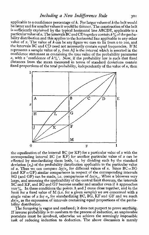
CONFIDENCE INTERVALSLet us assume that we have a probability law containing a parameter which

can take any value in a continuum limited at both ends (e.g. o to 1). The diagram is arranged to indicate the possible values of the parameter (x) on the vertical axis and the possible sample values (y) on the horizonta1 axis—the samples are assumed to be all of the same number. It is further assumed that the ‘expected’ or mean sample value is equal to x. Then the diagonal line between the axes represents the mean values applicable to the successive values of x.

The curved lines are a sufficient representation of the confidence belt

Including a New Indifference Rule 301 applicable to a confidence percentage of k. For larger values of k the belt would be fatter and for smaller values it would be thinner. The construction of the belt is sufficiently explained by the typical horizontal line ABCDE, applicable to a particular value of x. The intervals BC and CD together contain k% of the probability distribution and this applies to the horizontal line applicable to any other value of x. The value of k can be any figure we care to fix from o to 100, and the intervals BC and CD need not necessarily contain equal frequencies. If M represents a sample value of y, then AJ is the interval which is asserted in the confidence statement as containing the true value of the probability parameter x, with a ‘confidence of k%'. Now, if the probability law is such that fixed distances from the mean measured in terms of standard deviations contain fixed proportions of the total probability, independently of the value of x, then

the equalization of the interval BC (or KF) for a particular value of x with the corresponding interval BC (or KF) for another particular value of x can be effected by standardizing them both, i.e. by dividing each by the standard deviation ( x) of the probability distribution applicable to the particular value of x. Thus we can compare y/ x for different values of x. Since BC = BG (and KF = GF) similar comparisons in respect of the corresponding intervals BG (and GF) can be made, i.e. comparisons of x/ x. When n becomes very large, and assuming the applicability of the central limit theorem, the intervals BC and KF, and BG and GF become smaller and smaller even if k approaches 100%. In these conditions the points A and J come close together, and in thelimit for a fixed value of M (i.e. for a given sample) we are concerned with a single value of x for x for standardizing BC, BG, KF and GF and we reach dx/ x as the expression of intervals containing equal proportions of the probability distribution.

The foregoing is vague and confused; it does not purport to prove anything. If inverse probability is to conform to the process of induction, an unprovable postulate must be involved, otherwise we achieve the seemingly impossible task of reducing induction to deduction. The above discussion is merely

302 Some Observations on Inverse Probability intended to indicate the line of intuitive thought which first suggested the new indifference rule. I had in mind that, for a fixed standard deviation, the confidence belt applicable to the mean of a normal universe is a pair of straight lines parallel to the diagonal between the x and y axes. For different values of k, we have a sort of mesh of parallel probability lines. In this case, the uniform distribution of the prior probabilities works well and gives the same results as the confidence statement. A similar position seems to arise with the t-distribution, provided that Jeffreys’s rule is used for the prior probabilities applicable to the standard deviation parameter. This suggests that in other problems in order to obtain the same equivalence we need to transform the parameter so that the confidence belt takes a similar parallel form. In large samples, this is just what the new rule achieves in conditions in which the central limit theorem applies (it is worth noting that Whittaker in his paper repeatedly stresses the assumption of ‘statistical regularity’), and it is precisely the extreme cases of the large sample results of the Bayes-Laplace rule applied to the probability parameter in the binomial law which have been impugned as unreasonable. The use of the same rule for small samples seems to be a reasonable postulate to make, because there is no reason to adopt a different prior probability distribution as between large and small samples. Our prior attitude to the various possible values of the unknown parameter is the same in both cases. It may be observed that a very lucid and precise treatment of confidence intervals is contained in Chapter VI of Wilks’s Mathematical Statistics and that their equivalence with the results of inverse probability on the new indifference rule in the case of large samples seems to be implied in the results obtained by the appeal to the central limit theorem on pp. 127–130.

The idea of the confidence interval diagram as a probability mesh and the need to secure parallelism by transformation gives support to the idea that the problem is basically similar to that of the ‘world structure’ in relativity theory. In the case of the binomial probability parameter, the transformation to a uniform distribution of prior probabilities round a full circle suggests a confidence picture in the form of a sphere with an orthogonal mesh of great circles, generated by rotating two planes at right angles to each other (one for the parameter and the other for sample values , where sin = 8y ( 1 -y) - 1). The confidence lines for large samples would then be lines of latitude parallel to an ‘equator‘.

SOME RESULTS BY THE NEW RULE If we have made n drawings from a binomial universe and have achieved m

successes, then the new rule pxdx = dx/ x½ (1 - x)½ yields the following distribution of the posterior probabilities

The mean value of this distribution, which is the total, posterior probability of the next trial being a success, works out at (m + ½)/(n + 1) compared with the Bayes-Laplace result (m + 1)/(% + 2).

The maximum posterior probability works out at (m - ½)/(n - 1), compared with the Bayes-Laplace result ( = the maximum likelihood value) of. m/n. If m = n, the maximum posterior probability is, of course, 1. If m = o, the maximum posterior probability is o. If we desire to make a point estimate of the parameter,

Including a New Indifference Rule 303 the maximum posterior probability would be the appropriate choice. If, however, we want to obtain a pair of limits containing the ‘true’ value with a fixed posterior probability A say, we must evaluate a and b in the integral

and no doubt we should wish to minimize (b-a).

It is worth noting that if we assume that x is such that our sample result m/n is the most probable result (i.e. the mode of the binomial distribution (x + 1-X)n) the possible values of x range from m/(n + 1) to (m + 1)/(n + 1). The mean value or the value in the middle of the range of these possible values is, of course, (m + ½)/(n + 1). This result lends some support to the value given by the new rule for the probability at the next trial as a ‘not unreasonable’ result. Actually m/n lies between (m + ½)/(n + 1) and (m - ½)/(n - 1). For those who have an instinctive feeling for m/n as the ‘best’ estimate, there is perhaps some point in asking why they prefer to identify the sample result with the mean rather than with the mode. It seems to be precisely because the binomial law is a discrete probability law with slightly discrepant mean and mode that all the mathematical difficulty in applying inverse probability to this case has arisen.

If m = ½n, the total posterior probability of success next time is .5 so that the rule conforms to the obvious position that we still have no reason to favour success rather than failure.

If m = n, the total posterior probability of success next time is (n + ½)/(n + 1) compared with the Bayes-Laplace result (n + 1)/(n + 2). This provides a new rule of succession and expresses a ‘reasonable’ position to take up, namely, that after an unbroken run of n successes we assume a probability for the next trial equivalent to the assumption that we are about half-way through an average run, i.e. that we expect a failure once in (2n + 2) trials. The Bayes-Laplace rule implies that we are about at the end of an average run or that we expect a failure once in (n + 2) trials. The comparison clearly favours the new result from the point of view of ‘reasonableness’.

If m=o, the total posterior probability of success next time works out at ½/(n + 1), wh h ic is a much more reasonably remote result than the Bayes- Laplace result 1/(n + 2).

As mentioned earlier, the indifference rule considered by Jeffreys (i.e. pxdx dx/x (1 - x)) to go too far in the other direction, compared with Bayes- Laplace, produces m/n for the total posterior probability of success at the next trial. Thus, the results of the new rule lie ‘reasonably’ between the two extremes.

On the Bayes-Laplace basis, K. Pearson produced the result that after n successes in n trials the total posterior probability that the next (n + 1) trials will all be successes is exactly .5, whatever the value of n.

On the new rule the corresponding probability that the next n will all be successes is

Putting n = 1, 2, 3, . . . , successively we obtain the results 3/4, 35/48, 693/960, . . . , rapidly tending to the limiting value of 1/ 2 as n tends to infinity. This is clearly more ‘reasonable’ than either the Bayes-Laplace result or the result on the alternative rule rejected by Jeffreys which gives certainty as the probability. It clearly provides a very much better correspondence with the process of induction. Whether it is ‘absolutely’ reasonable for the purpose, i.e. whether it is yet large enough, without the absurdity of reaching unity, is a

304 Some Observations on Inverse Probability matter for others to decide. But it must be realized that the result depends on the assumption of complete indifference and absence of knowledge prior to the sampling experiment. When this assumption is not appropriate other con- siderations apply, and some discussion of this aspect is given in the next section. One other result in this connexion may be of interest. The new rule yields .5 as the total posterior probability that the next 3n trials will all be successes, after having obtained n successes in n trials. In this form, the new rule certainly seems to have gone a long way to dispose of one of the principal objections to inverse probability, namely that the Bayes-Laplace rule of succession produces results which do not correspond with anybody’s way of thinking.

It is worth noting that the new result (m + ½)/(n + 1) conforms to the general form quoted by Jeffreys as obtained by W. E. Johnson, namely (m + k)/(n + 2k). It also fits Makeham’s empirical ‘general’ formula (m + rp)/(n +r) (J.I.A. Vol. XXIX, p. 250). Unfortunately, Makeham’s work is marred by serious confusions of thought. At that time? because of the constant reference to balls in urns there had often been a confusion. between the prior probability distribution and the prior probability of each particular ball being of a particular colour. Makeham speaks of p as the ‘antecedent probability’ but goes on to treat it also as the unknown universe parameter. This confusion is pursued in a note by E. L. Stabler(J.I.A. Vol. xxx, p. 239). Having regard to the way in which Makeham reached his ‘general’ formula, it is remarkable that it covers all the cases which can arise from Hardy’s form xr (1+ x)s for the prior probabilities.

It is plain that the results of the new rule differ but little from the classical results. It would be illogical, however, for those who object to inverse probability because of the results yielded by the Bayes-Laplace rule, to object to the new rule on the basis that the modifications necessary to reach 'reasonable’ and consistent results are very small. As Jeffreys has pointed out, the effect of any normal change in the prior probability distribution is equivalent to the effect of one more observation and is a fraction only of the statistical uncertainty of the result. The discrepancies have been arithmetically minute, but the theoretical difficulties have profoundly retarded the development of the fertile seeds sown by Bayes and Laplace and only in recent years nursed into maturity by Jeffreys.

THE PROBLEM OF COMPOUND EVENTS, ASYMMETRICALALTERNATIVES AND ‘THE MIDDLE’

It has long been known (e.g. see Keynes) that the application of the same indifference rule to compound events as to the elementary events of which they are compounded produces inconsistent results. On the basis of the Bayes- Laplace rule, if we have had n successes in n trials, the probability that the next n trials will all be successes is 2/3 for n= 1, 3/5 for n=2, 4/7 for n= 3, rapidly tending to 5 as n becomes large. If now we regard n trials as a single compound trial, n successes in the n trials as a single compound success, and one or more failures in n trials as a single compound failure, and apply the Bayes-Laplace indifference rule to these compound events, the probability of n successes in n trials after n successes in n trials becomes the probability of 1 compound success in 1 trial after 1 compound success in 1 trial, and the inconsistent answer of 2/3 results whatever the value of n. The reason for the inconsistency is obvious: the application of the Bayes-Laplace indifference rule both to elementary and to compound events represents two different postulates.

The new rule does not, of course, avoid this inconsistency, although the


discrepancy is considerably reduced. The corresponding results as already indicated are 3/4 for n= 1, 35/48 for n=2, 231/320 for n=3, rapidly tending to 1/42 ( .707) as n becomes large.

Let us consider the basis for adopting an indifference rule at all. It is assumed that before taking a sample we have the possibility of only two alternatives and that we have no reason whatever to suppose that one alternative is more likely to occur than another. This attitude of mind would seem to be appropriate only if the two alternatives are logically symmetrical. This idea of logical symmetry may be illustrated in the following way. If an urn can contain only two kinds of balls, white and red, in unknown proportions, the alternatives white and red are logically symmetrical. If, on the other hand, the urn contains white and not- white balls (i.e. balls of any colour other than white), the alternatives white and not-white are logically asymmetrical. That the, assumption of ‘indifference’ between two alternatives is reasonable only when they are symmetrical has been pointed out by a number of writers on inverse probability. It is precisely for this reason that when we are dealing with compound events it is inappropriate to adopt an indifference rule for their prior probabilities. The alternatives— n successes (or failures) and one or more failures (or successes)-are clearly asymmetrical. If this distinction is maintained and the indifference rule is confined to elementary symmetrical events the inconsistencies are avoided and we have to seek some other ay of dealing with asymmetrical alternatives.

Now let us consider the possibilities of biased rules for the prior probabilities. If we assume pxdx dx/x as the expression of a biased rule and write y=xn, corresponding to a compound success made up of n sub-events, we have dy = nxn-ldx so that pydy dy/xn = dy/y. Thus we can contemplate a chain of events, a compound event made up of sub-events, a sub-event made up of sub- sub-events, and so on, and at each stage we have a biased prior probability rule in the same form dx/x. Similarly, if we assume pxdx dx/(1 - x) as the expression of bias in the other direction and write (1 - y) = (1 - x)n, we have

and pydy dy/(1-y), with a corresponding chain of rules of the same form. These two biased rules dx/x and dx/(1- ) x represent the two limiting cases of

the general expression dx/x1-r (1 - x)r which includes the new indifference rule as a special case when r = ½. The mean value of the distribution dx/xl-r (1 - x)r is r, so that this rule is a convenient way of giving the mildest possible preference to the value x = r before taking the sample, without reaching unreasonable results.

Applying the rule dx/x, the total posterior probability of a success at the next trial, after m successes in n trials, is m/(n + 1). On the rule dx/(1 - x) this probability is (m + 1)/(n + 1). The former rule is a J-shaped curve expressing a bias in favour of x = o, while the latter expresses a bias in favour of x = 1. The very small difference between the resulting posterior probabilities (of the order of (a) the difference between the mean and the mode of the binomial distribution or (b) I/ n times the standard deviation of the binomial distribution) clearly illustrates the size of the gnat which the opponents of inverse probability are unable to swallow and also the pertinent remark by Jeffreys that the effect of any ordinary change in the prior probabilities is of the order of the effect of one more observation.

It is of interest to note that the arithmetic mean between the results of the two limiting biased rules is the same as the result of the new indifference rule. This suggests that if we know that our two alternatives are asymmetrical but

306 Some Observations on Inverse Probability have no reason to assign a ‘direction’ to the asymmetry, i.e. to choose which alternative to bias, we might apply to the two biased results the simple indifference rule of assuming them to be equally likely, i.e.

and so obtain the same result as using the new indifference rule at the beginning. In applying inverse probability to actual observations of natural events, we

are faced with the difficulty of determining which events are elementary and which are compound. It is one thing to speculate, as in certain modern philo- sophies, about a world structure made up of elemental events, but it is another to determine whether a particular defined event is elementary or compound. If we are sure that there are only two precisely defined alternatives and we have no reason to bias one way or the other, the line of argument in the preceding paragraph may resolve the difficulty. It seems clear, however, that in the scientific sphere the problem often poses itself inescapably in one of two forms; either there is a ‘middle’ which we cannot entirely distribute in advance by definition of two symmetrical alternatives, or our alternatives are asymmetrical. This is particularly so at the microscopic level, and seems to be connected with the uncertainty principle in quantum physics. The following quotation from Reichenbach (loc. cit., p. 45) brings out the point clearly:

‘Now the results of quantum mechanics can be so interpreted that when we insist upon constructing the language of physics in a two-valued manner it will be impossible to satisfy the postulate of causality, even when an extension of causal connexions to probability connexions is admitted. The violations of the principle of causality are of another kind; they consist in the appearance of an action at a distance. On the other hand, it can be shown that causal anomalies disappear when the statements of quantum mechanics are incorporated into a three-valued logic. Between true and false statements we then shall have indeterminate statements; and the methods by which the truth-values of statements are derived from empirical observations are so constructed that they will classify any quantum mechanical statement in one of the three categories.’

We are familiar with the notion that our knowledge of the external world is never certain. Whitehead (loc. cit., p. 30) says ‘But in general, with more complex instances, complete certainty is unattainable.’ Einstein quotes Hume as follows: ‘Whatever in knowledge is of empirical origin is never certain.’ If, when we are considering two alternatives which cannot be precisely defined as symmetrical alternatives, we adopt the rule dx/(1 - x) for the prior probability of success A (failure being not-A), and also the rule dx/x for the prior probability of failure B (success being not-B), where (A + B) is not exhaustive and does not therefore succeed in distributing the ‘middle’, we bias our prior probabilities in each case in favour of the alternative which includes the ‘middle’. We then obtain for our posterior probabilities, after m cases of A and (n -m) cases of B in n trials, the values m/(n + 1) and (n - m)/(n + 1) We thus leave a probability of 1/(n + 1) as the expression of the limit of uncertainty to cover the ‘middle’ and of the fact that we can not be sure that a third alternative ‘neither A nor B’ will not turn up, however large n may be. If we distribute the ‘middle’ equally between the two we return to the results by the new indifference rule. Is it mere nonsense to suggest that in some such way the theory of inverse probability may be made to embrace the principle of uncertainty in quantum physics or that the idea of the elementary event and the quantum of action are

Including a New Indifference Rule 307 associated? It may be so, but that philosophy, inductive logic, quantum theory and probability theory are all intimately interlocked is a commonplace of modern thought.

The above suggestions for dealing with asymmetrical alternatives or the ‘middle’ have the merit that the same process can be employed when there are any number of alternatives and an undistributed middle. Thus if out of n trials we have m1, m2, m3,... results of the various kinds and no case of the ‘middle’, a separate application of the dx/x rule to each alternative yields m1/(n + 1), m2/(n + 1), etc., leaving 1/(n + 1) for the middle. The combination of two or more alternatives and the use of the dx/x rule yields (m1 + m2 + . . . )/(n + 1) and the whole system is consistent.

There is one other application of the biased rules which is worth mentioning. If we have developed a hypothesis by reasoning from known ‘facts’ and from other well-supported theories and have devised an experiment to test its truth, a single success will usually clinch the matter from the practical point of view, If in such circumstances we adopt the rule dx/( 1 - x), our total posterior probability is always certainty, until we get a failure in the routine, when the rule gives appropriate expression to the probability of success next time. If, on the other hand, we pose a hypothesis which we have every reason to regard with suspicion, the adoption of the rule dx/x will produce a posterior probability of zero until a success appears. These results seem to bring within the scope of inverse probability the probability basis of the scientific process of well- designed experiment to test hypotheses with high or low prior probability.

The fact that by appropriate choice of the prior probability we can range from extreme bias in one direction through indifference to extreme bias in the other direction and obtain ‘acceptable’ results differing between the extremes by 1/(n + 1) only is surely an advantage over the direct systems, which like indifference rules are designed as processes for allowing the statistics to speak for themselves. At any rate it is clear that the maximum likelihood solution (m/n) outrages reasonable belief when m = n. One remarkable feature of the results by the two extreme prior probability rules is that they coincide with the extreme values of x which yield the mode for the sample value, while, as has been already mentioned, the new indifference rule produces the mean value of all possible values of x which result from identifying the sample value with the mode.

THE PROBLEM OF MULTIPLE SYMMETRICAL ALTERNATIVES

The solution of the binomial problem and the discussion of the problem of asymmetrical alternatives have suggested a general solution of the case of multiple symmetrical alternatives, i.e. the multinomial problem. This problem was examined by Lidstone (T.F.A. Vol. VIII, p. 182). He extended the Bayes- Laplace postulate, giving all possible distributions of the multiple parameters (x1 + x2 + x3 + . . . + xi = 1) equal prior probabilities. If we divide the alternatives into two groups of equal number

(e.g.thus reducing the problem to the binomial case with symmetrical alternatives,alternatives, the extended postulate does not reduce to a uniform prior probability distribution of y. The resulting distribution is heaped up towards y = 5 and the heaping up increases as i increases. There is thus a critical inconsistency between the multinomial and binomial cases if the uniform distribution is used for both.

AJ 20

and

308 Some Observations on Inverse Probability This inconsistency is shown clearly in the posterior probability produced by Lidstone. If in n trials there have been m1, m2, . . . , mt, . . . , mi results of the various possible kinds, Lidstone’s result (given also by Jeffreys, p. 113) is (mt + 1)/(n + i) for the posterior probability of a result of kind t at the next trial. It is clear that the posterior probability of a result of any kind from x1 to xi/2 at the next trial is then (m1 + m2 + . . . + mi/2 + i/2)/(n + i) compared with the direct binomial result, on the Bayes-Laplace postulate, of

In fact for large i the usual result given by Lidstone and Jeffreys is quite unacceptable from the point of view of reasonableness and consistency.

Now, if, instead of adopting the Bayes-Laplace postulate for the prior probabilities of a given alternative, we treat the problem as one of two asymmetrical alternatives for which, as there are i component alternatives altogether, we require a prior probability distribution with a mean value of 1/i, we can use the rule px dxdx/x1–r (1–x)r and put r = 1/i. Given, therefore, n trials with mt results of a particular kind out of i kinds, this rule yields (m1 + 1/i)/(n + 1) as the posterior probability of a result of this particular kind at the next trial. More- over, if we select k component alternatives as a group of successes and the remaining (i-k) component alternatives as a group of failures, the appropriate rule dx/x1-k/i ( 1 - x)k/i yields the result (m + k/i)/(n + 1). These results are completely consistent inter se and with the binomial case of two symmetrical alternatives. The entire results lie between the extremes m/(n + 1) and (m + 1)/(n + 1) and in the limit when i tends to infinity and k tends to zero we reach the limit of bias represented by the rule dx/x. At the other extreme, when k tends to infinity with i, we reach the other limit of bias represented by the rule dx/( 1 - x).

It remains to consider the meaning of these results and the underlying composite prior probability distribution. Consider the original binomial rule pxdx dx/x½ (1 - x)½ . This may be regarded as a case of two related parameters, x1 and x2, where x1 + x2 = 1. We can therefore write the original rule in the form

where x1 + x2 = l. This suggests that for the case of multiple symmetrical alternatives we should

adopt the rule

where We can now suppress xi and give effect to the equation of condition by writing

Following the example given by Lidstone (loc. cit., p. 184), and integrating with respect to xi-1 and putting y = xi–1/(1–x1–x2–…–xi–2) so thatdxi–1 = dy(1–x1–x2–…–xi–2), we obtain

Including a New Indifference Rule 309 Proceeding in this way to eliminate stage by stage all the variables except x1 we arrive finally at the result

which is the form used above for the case of two asymmetrical alternatives. If we stop eliminating variables at the previous stage we have

By putting x1 + x2 = y we can obtain the distribution appropriate to y as follows :

Writing so that dx, = ydz we reach

In a similar way it can be shown that if y = x1 + x2 + . . . + xk the distribution of y is which is the form used above for grouping the alternatives

into two groups. The general rule px1x2 . . . dx1 dx2 ...dx1dx2 ... /xlx2 . . . subject to the con-

dition x1+x2+...= 1 covers all the cases considered. The prior probability rule used in the above development for the multiple

parameters in the multinomial distribution seems to have its interpretation in terms of co-variance of the second order, that is, in terms of the square root of the second order product-moment ( µ2. 2. 2... (i terms)) ½ , which for large samples is proportionate to xl x2x8 . . . xi . In the case of independent variables, the second order co-variance reduces to the product of the separate variances and there is no conflict with Jeffreys’s practice (or the principle of the product rule) of multiplying together the prior probabilities of two or more independent parameters.

I have not succeeded in obtaining an interpretation of the multiple parameter rule in terms of circular measure to parallel the uniform distribution of angles for the binomial case.

THE CASE OF TIME RATES Time rates (e.g. mortality rates and most other actuarial rates) are clearly

concerned with compound events. Survival is a continuing process and we can subdivide our time interval indefinitely. The difficulties arising out of this feature have been discussed by Hardy, Lidstone and others (T.F.A. Vol. VIII, pp. 174, 195); and Calderon (J.I.A. Vol. xxxv, p. 170) has endeavoured to meet the difficulty by defining an elementary time interval as the average time required in a given experience to cover exactly one death. Jeffreys uses the rule dx/x for such cases, following the example of Haldane who used this rule for the problem

20-2

310 Some Observations on Inverse Probability of estimating the rate of emission of particles from radioactive material. If we assume that the probability law, when the time interval is made very short, is the Poisson distribution, and adopt the new indifference rule, we obtain dx/x½ for the prior probabilities, where x is the unknown Poisson parameter. The resulting mean posterior probability is ( + ½ )/nE, where is the observed number of events (e.g. deaths), E is the exposed to risk in years and n is the number of unit time intervals in a year. Clearly the difficulty discussed by Hardy remains. The difficulty is, however, resolved by appreciating that time rates involve asymmetrical compound events, so that indifference is inappropriate. Remembering that our time interval is reduced indefinitely, the parameter x must be known to be biased towards zero. If it were not so, we should not be sampling at all because the whole system would take on an ‘explosive’ character. Thus the conditions suggest the biased rule dx/x in support of Haldane’s assumption. The mean posterior probability is then /nE whatever time unit we use and Hardy’s difficulties disappear. Thus, in effect, for time rates we return full circle to m/n as our estimate.

CONCLUSION It is obvious that in writing this paper I am greatly indebted to Jeffreys’s

work. I am also indebted to various members of the Institute with whom I have discussed probability questions from time to time and in particular to Mr H. Hosking Tayler with whom I carried on a long correspondence on philosophic aspects of probability theory, but I do not suggest that they support inverse probability in general or any part of this paper in particular. Whatever there may be in the paper of worth which has its origin elsewhere, I alone am re- sponsible for any mistakes and in particular for the somewhat reckless and ill-informed excursions outside my limited actuarial sphere. In permitting these excursions to appear at all, I have had in mind the motto which is reputed to have appeared in Government Offices in America during the war— ‘ Remember that the turtle makes progress only when he sticks his neck out’.

Including a New Indifference Rule

… (1)

311

ADDENDUM When the first proofs of this paper became available I sent a copy to Prof.

Jeffreys who kindly supplied me with a copy of a paper of his own which had appeared a week earlier (mid-October 1946) in the Proceedings of the Royal Society. This paper, entitled An invariant form for the prior probability in estimation problems, adopts a somewhat different and more general approach to the problem of an invariant rule. He reaches the same prior probability distributions for the binomial and Poisson laws as I do, but he does not give any posterior results or discuss the problem of asymmetrical alternatives, compound events and the ‘middle’, or time rates or the multinomial distribution. I understand that he has done further work on the subject which has not yet been published.

Also while this paper was in the hands of the printers Vol. II of Kendall’s Advanced Theory of Statistics appeared. In Chap. 20 he discusses the various cases in which Jeffreys’s results are identical with Fisher’s fiducial distributions and raises the question of what prior probability distribution of the correlation parameter in a normal distribution would be necessary to produce a posterior probability distribution for p which would be identical with the fiducial distribution. The prior probability distribution of p by my new rule is dp/(1 – p2). If we apply Fisher’s transformation

the distribution of is uniform, as is obvious from the fact that the large sample standard error of z (where z = tanh-1 r = ½ {loge (1 + r) –loge (1 –r)}) is independent of

Now Jeffreys gives Fisher’s distribution of r in the form

where Sn–1 (pr) is a series in terms of (pr) and n, which is barely distinguishable from unity for quite small values of n.

On applying the and z transformations and following Jeffreys’s procedure we obtain the distribution for x

Since the prior probability distribution of 5 is uniform, the substitution in (1) of d for dz produces the posterior probability distribution of

Now, as n increases, Sn–1, tends to unity and the product of the first two terms in the denominator over the significant part of the ranges of and z also tends to unity. It therefore appears that for large n the fiducial distribution is identical with the posterior distribution. Unfortunately, Kendall does not give the fiducial distribution which he discusses, and I confess to having an insufficient understanding of fiducial probability even to be sure whether there is an explicit fiducial distribution in this case for small n, notwithstanding that r is sufficient for p and z for

The point is important because of the general question of whether inverse probability, while having a much wider field of application, can be shown to embrace fiducial probability in all cases, both for large and for small samples.

312 Some Observations on Inverse Probability It will be seen that the maximum likelihood and the maximum posterior

probability of are identical, as obviously will be so in all cases where a transformation is made so that the prior probability distribution of the transformed parameter is uniform. Unlike the maximum posterior probability, the maximum likelihood is invariant to transformation, because the likelihood does not include the differential elements. It might be. suggested that this invariant property confers on the maximum likelihood a superiority in principle over the maximum posterior probability, but my own view, for what it is worth, is that an estimate should have regard both to the basic assumptions regarding prior knowledge (i.e. indifference or specific bias) and to the purpose of the estimate. If we desire to estimate x, we naturally wish to obtain the most probable value of x and not the most probable value of y, where y = f (x) is the transformation necessary to produce a uniform prior probability distribution. In those cases where fiducial probability and posterior probability based on the new indifference rule are identical, interval estimations by the two methods are identical, although if ‘ shortest interval ’ estimation is desired, we again have to select the form in which to express the parameter by reference to our purpose, because shortest intervals are not invariant under transformation.

Finally, the transformation relation of my new indifference rule will be recognized as being identical in form with Fisher’s rule for obtaining the ‘ amount of information’ (Im) with respect to m from the ‘amount of information ’ (I,) with respect top, where p is a function of m. This is given on p. 209 of The Design of Experiments as follows:

Im and Ip respectively being defined as the reciprocals of the sampling variances,

so that


ABSTRACT OF THE DISCUSSION Mr Wilfred Perks, in introducing the paper, explained that after studying

Prof. H. Jeffreys’s paper in the Proceedings of the Royal Society and the early chapters of Vol. 11 of M. G. Kendall’s Advanced Theory of Statistics, both of which had appeared after his paper was written, he had reached the conclusion that the new indifference rule might be better expressed in terms of the square root of the minimum variance integral. That would have the advantage of making the rule more definite and precise without altering its essential content and properties and without making any change in the particular cases discussed in the paper. M. G. Kendall showed in his book that in certain cases fiducial probability and inverse probability were equivalent. He personally thought that a degree of equivalence might be shown also in the binomial case. He had somehow missed in the literature the expression for the tail of a binomial distribution in the form of the incomplete beta function, which showed that the construction of a posterior probability belt on the biased rule dx/x produced the lower curve in the binomial confidence belt, whilst the rule dx/(1– x) yielded the upper curve. The interesting thing was that the new indifference rule which arose from his general rule and also from Prof. Jeffreys’s invariant rule produced a posterior probability belt which lay snugly just inside the confidence belt. It would be remembered that the confidence belt gave a probability inequality, whereas the posterior probability belt purported to give a probability equality. That seemed to suggest that inverse probability and the direct methods might be made equivalent in the binomial case, bearing in mind that m/n was a sufficient statistic.

He wished particularly to refer to the illustration of the obscured die on p. 291, because he felt he had not brought out the point sufficiently clearly. If he invited someone to call heads or tails to the tossing of a coin at even odds, it would not matter to that person whether he called before or after the coin was tossed. Even if the coin were laid upon the table it would still be a fair bet. The same applied to odds of g to I against a specified digit in the case of a digit from a set of random numbers or in a particular decimal place in provided that the caller did not know the answer. It was precisely that type of case which the modern schools of probability excluded from their theories; but it seemed to him that a unified theory of probability was bound to include such cases if it was to provide a basis for scientific method and induction. Hume’s analysis of the induction problem had, as far as he knew, never been broken. Induction could not be developed solely out of the usual logical principles. Russell’s verdict in History of Western Philosophy, published about two months previously, was that induction was an independent logical principle incapable of being inferred either from experience or from other logical principles, and that without that principle science was impossible. To bring that principle into the body of probability theory an independent postulate was required which had to be consistent with the direct probability of pure mathematics. An independent postulate which was consistent with the direct probability of pure mathematics was the object of importing an invariant indifference rule.

Dr L. Solomon, F.F.A., in opening the discussion, said that the main subject of the paper— important to actuaries as well as to statisticians— was estimation. As a simple example, there was the familiar problem: If m lives died out of n exposed to risk, what could be said about the rate of mortality-about what used to be called the ‘true underlying’ rate? Several systems had been developed for providing answers to that type of question. The author had ardently embraced one of those systems and had classed the rest as heresies. Without going into lengthy detail, he could only state his contrary opinion that several independent theories, logically sound and self- consistent, could exist dealing with the subject of probability, just as several geometries existed. He believed, too, that more than one consistent and practical system of estimation could be built up on them. The author had not been wholly fair to the confidence interval method or the fiducial probability method of estimation, and he considered

314 Some Observations on Inverse Probability that the author’s strictures against the frequency and measure theories of probability would not seriously endanger them.

The differences between the several theories arose in the first instance from the old arguments about the scope of probability, to which the author had briefly referred. There were such statements as: ‘ Burma will be an independent republic within six months ‘, ‘ The decimal in the 950th place of is 3 ‘, or ‘ The philosopher Gionardo Bruno had blue eyes ‘. What was the probability that each of those was true? If probability were interpreted as a measure of belief, it was possible in principle to give an answer. The statistician who adopted the frequency theory, however, regarded those questions as meaningless, and was not seriously embarrassed by his inability to answer them. It was the same difference in attitude that arose with regard to the concept of prior probability distributions, especially when arguing inductively from the result of a single experiment. If there were n lives exposed to risk, the actuary postulated that they were all subject to a uniform rate of mortality, q. Most people would agree that it was useful to consider those n lives as a random sample from a hypothetical universe containing an infinite number of lives all subject to the same q. The inverse probability stand-point could be summarized thus: ‘Before we start to experiment or observe we must know the probability that the true q lies within any prescribed limits. Then we use the results of observation and experiment to modify such prior probabilities and to obtain the so-called posterior probability distribution. By operations upon the posterior distribution we are able to answer various questions and make various predictions.’ The opposing point of view, i.e. that of the frequency school, regarded the idea of a prior distribution as involving a whole infinite population of populations, each member possessing its own appropriate true value of q; that idea he found, in very many cases at least, unacceptable, and even meaningless. The frequency school proceeded to develop other methods of making inductive statements-‘direct systems’, as the author called them-which enabled consistent and useful statements and predictions to be made and which successfully circumvented the difficulties of the prior probability distribution.

He wished to explain what he meant by ‘ circumvent ‘. If there were no prior probability distribution for the parameter in question, the direct systems provided a rational means of answering practical questions. In certain cases, moreover, especially when repeated experiments were involved, the idea of the prior distribution might be acceptable to the statistician-the supporter of the frequency school-but the mathematical form of the prior probability might be unknown to him. In that case the direct systems still satisfied the criteria they were designed to satisfy. From that point of view they were invariant to the mathematical form of prior probability distribution. He suggested, therefore, that if a person had any doubt whatever about the legitimacy of the prior probability concept he was bound to accept one of the direct systems. On the other hand, if he found he could embrace the faith of inverse probability, he would doubtless find the solace and the satisfaction which he deserved. That difference in attitude had led in the past to much argument, brilliant debate and bitter invective. It was a pity from some points of view that the supporters of those two separate, self-consistent theories could not go their separate ways, in peace.

He had used the expression ‘self-consistent’. That was the key to much of the author’s work. In the practical application of his ideas the prior probability concept was not enough; it was necessary to use a specific mathematical formula which expressed the nature of the prior knowledge or, as was so often the case, of the prior ignorance. One such formula was embodied in the famous Bayes’s postulate, but although that seemed logically satisfying to some it led, as the paper showed, to inconsistencies. The main merit of the paper was that it put forward an alternative which successfully avoided one group of inconsistencies, namely those associated with transformation of the parameters which were to be estimated. The new indifference rule was arbitrary in form and it was expressed with perhaps misleading symmetry. At the foot of p. 296 the x in was not the same as the x appearing elsewhere. The x in was that function of the observations which was used to estimate the parameter referred to by the other x on the left-hand side of the relation. As for the estimating

Including a New Indifference Rule 315 function, the author had suggested the sufficient statistic when it existed. That was fair enough, since the existence and the form of the sufficient statistic was independent of the prior probability distribution. Indeed a supporter of the frequency school might think that having found the sufficient statistic he had completed his job. That enabled him to answer all the questions which arose in practice and he might go so far as to regard the author’s indifference rule with complete indifference! As for the distributions which did not admit of a sufficient statistic, he was not at all clear what should be done. The author had suggested the use of whatever consistent statistic was finally adopted, but how was one to know which consistent statistic to use without working out the posterior probability on the basis of the specific prior distribution or without bringing in alien criteria?

Apart from that difficulty-and perhaps the author would remove it-he was not worried by the arbitrary nature of the new indifference rule. It might, however, be worth stressing the statement that the intuitive arguments on pp. 300–302 proved nothing. All methods of estimation contained an arbitrary element, largely because there were no universally accepted rules of inductive logic. Since an arbitrary formula had to be adopted, it seemed reasonable to adopt one which removed some of the posterior inconsistencies. That was, in fact, the achievement in the first part of the paper, and, viewed in its proper focus, it was a very solid and valuable achievement.

He had one more comment to make on that section of the paper, and perhaps it was somewhat of a debating point. The author had repeatedly quoted Prof. Jeffreys’s observation that the numerical effect of a change in the prior probability was trivial. He could not quite reconcile that with two other statements. The Bayes-Laplace rule was said to produce results which ‘ do not correspond with anybody’s way of thinking’, whereas a change in the prior probability distribution produced the author’s indifference rule, which was put forward as eminently acceptable.

He found the second part of the paper, i.e. that dealing with compound events, asymmetrical alternatives and the multinomial distribution, exciting, stimulating, but far from clear. As he saw it, in certain experiments prior knowledge was available as a guide, and full use had to be made of it; in inverse probability terms, a biased probability distribution was used. That had led the author to discuss logically asymmetrical alternatives, which he had illustrated but not explained. Again, on p. 305 the author had quoted the basis for applying an indifference rule, but personally he did not see how that basis allowed an indifference rule to be applied to estimate, for example, the parameters of a normal distribution. Yet that had been done in the earlier part of the paper.

One formula was quoted on p. 305 from the infinity of possible forms which might express bias. A special case of that formula was the binomial indifference rule, and the two extreme cases were obviously of particular importance because they were discussed fully later on. He admitted the algebraic convenience of the author’s formula, but asked in what way it really did express the bias that existed in the type of problem under discussion. Furthermore, the formula contained the index r, and it was stated that by using the index r the mildest possible bias was given to a preconceived idea that x = r. Why was it the ‘mildest possible’ bias?

With regard to the two extreme cases, expressed by dx/x and dx/( 1 – x), there would seem first to be a convergence difficulty if they were treated as probability distributions over the whole range 0–1, and if dx/x were used it seemed to give to small values of x a tremendous bias rather than the mildest possible bias. The virtue of those forms, of course, was that they were invariant under some -though not all-transformations of the parameter. That made them convenient or attractive for use in problems where it was virtually certain that a correct prediction would be made, e.g. in discussing the probability that the sun would rise tomorrow or that the result of a physical experiment would be consistent with the second law of thermodynamics. They did not, however, apply to problems of near certainty, and they would not be appropriate in discussing, say, the probability that there would be no insolvencies among insurance companies in the following year. Thus far he thought he could see the main line of argument, though he had difficulty over details; but at the foot of p. 306 there followed an example which

316 Some Observations on Inverse Probability left a probability of 1/(n+ 1) unaccounted for. To his inexpert first glance that seemed to reflect a mere inconsistency of specification, but apparently that was not so. It appeared to have deep philosophical significance; it had affinities with tripartite logics and with the quantum theory. He was puzzled, especially by the last analogy. The ‘uncertainty principle’ in quantum mechanics stated that the product of two measured quantities should be less than a fixed constant. The author’s ‘middle’, if he might so describe it, tended to zero with n, the number of observations. He thought that many of the analogies in the paper were incomplete, and he was not convinced of the relevance of some of them.

Mr H. W. Haycocks said it was unfortunate that the paper did not give a precise definition of probability. He did not think it was mere coincidence that both Keynes and Jeffreys had also been criticized on those grounds. Both Russell and Ramsey had remarked that Keynes left an uncomfortable gap between probability and fact, so that it was far from clear why a rational man would act upon probability. More recently, Prof. Carnap, in a paper entitled Two concepts of probability, had remarked that the axiom system of Prof. Jeffreys’s recent theory was so weak that it did not constitute an explicit definition of probability.

It was clear from the paper that the author was concerned with some logical concept which could be called for the time being ‘logical probability‘. In fact, it was necessary to go to the philosophers and logicians to get some idea of the concept he had in mind. The point at issue emerged clearly from the statement to which the author had referred in his introductory remarks, i.e. Russell’s statement on Hume, in which Russell said that the most important section of Hume’s treatise was the one called Of knowledge and probability. Russell said that by ‘probability’ Hume did not mean the sort of knowledge contained in the mathematical theory of probability. That knowledge was not itself probable in any special sense; it had as much certainty as knowledge could have. What Hume was concerned with was uncertain knowledge, such as was obtained from empirical data by inferences which were not demonstrative. Hume was concerned really with all forms of inference.

It was stated by Ramsey in his well-known essay on probability that there might well be two concepts of probability—one which was of interest to logicians and one which was of interest to statisticians and scientists. That suggestion had been taken up in much more detail by Prof. Carnap in his papers Inductive logic and Two concepts of probability. He styled one ‘logical probability’ and the other ‘frequency probability’. Logical probability he preferred to call ‘degree of confirmation’, and it measured a degree of partial implication between premises and conclusion. Thus it could be seen that there was a degree of partial implication between the two statements, ‘The penny will fall heads or tails’ and ‘The penny will fall heads’. If there were no reason to prefer either result, i.e. if the evidence in favour of heads was equal to that in favour of tails, the logical probability or degree of confirmation could be defined as one-half. That, however, said nothing whatever about relative frequency. Frequency probability, on the other hand, corresponded to what was meant in vague language by relative frequency in the long run. For a scientific theory a more precise definition was required, but a simple statement of probability in that sense was factual and empirical and said something about the facts of nature in the same way as did a scientific law.

He wished to examine the paper in the light of those remarks. The author had assumed a population having a distribution of known form. It was strange, bearing in mind that the author was considering the problems of induction, that he had given no clue as to the way in which scientists knew the form of the law they wished to test. The author had postulated a form of law, but the value of the parameter was unknown. He had then considered the possible range of the parameter and had given to each value within the range a weight which was a compound of so-called prior knowledge and a measure of the likelihood of a sample for that value of the parameter. He had thus set up a hypothetical parameter distribution and had taken the mean of that distribution as his estimate. It was important to note precisely what that distribution was. The variables were possible values of the parameter and the weights were what might be

Including a New Indifference Rule 317 termed the weight of the evidence which, so to speak, pointed to the particular value of the parameter. For instance, in the case of maximum likelihood the weights were simply the likelihoods; the prior distribution was ignored. If the value of the sample were taken as the value of the parameter, then a weight of 1 was given to the sample value and of zero to all the others. It was clear from the author’s illustrations that that method gave results which were very similar to the other so-called direct methods.

It would clarify the position to consider what was done with the estimate when it was obtained. If the probability law was to be more than merely descriptive, the insertion of the value of the parameter would enable the scientist to control future data; the law would enable him to predict relative frequencies in which he was interested. That was obviously the case in physics, biology and, he thought, in actuarial work. Thus the parameter was a physical constant like the gravitational constant or the specific heat constant.

Unfortunately, perhaps, those frequencies were often called probabilities, but, as he had explained, in ordinary usage the word ‘probability’ had two very different meanings. It added to the confusion when frequencies formed part of the evidence for logical probabilities. That gave rise to the idea that logical probability had some connexion with relative frequency and perhaps ought to be regarded as a relative frequency. The connexion lay in the possibility that a logical probability might be a relation between evidence containing a statement of relative frequency and a conclusion which might also refer to a relative frequency. He pointed out that the term ‘prior distribution of probabilities’ should not be used if probability were defined only as logical probability, for that would imply variables that were logical probabilities and weights that were also logical probabilities and would lead to the assertion that there was a relation between evidence and a degree of confirmation, which was a logical absurdity.

The greatest confusion of that kind arose in connexion with the binomial law, since there the parameter varied from o to 1 and was usually called a probability. It then happened that the posterior probability became identified with the value of the parameter, and the two different concepts became indistinguishable, thus leading to un- ending verbal argument. He thought that the author had fallen into that confusion. As an illustration, if two urns contained red and white balls, the first in equal proportions and the second in unknown proportions, he asked what was the degree of confirmation or logical probability between the evidence and the statement that a ball drawn at random would be red. In either case a reasonable answer would be one-half, which simply meant that the weight of evidence in favour of red was equal to the weight of evidence in favour of white. That was just a conventional definition. If, however, a probability law were required which would enable statements to be made about relative frequencies in large samples, then for the first urn he would adopt (½ + ½)n, that being an induction from experience. He regarded induction as one of the three fundamental bases of knowledge; the other two being perception and memory. Induction could be justified on the ground that it was found to be successful in practice. The adoption of the binomial law in the case of the first urn meant that the parameter of the law-he was not talking about the probability—was equal to one-half, and, as it happened, it was also equal to the degree of confirmation or logical probability as defined. In the case of the second urn, while the logical probability was one-half, he could only say with confidence that the law was of the binomial form. He could say nothing whatever about the parameter; it was impossible to estimate on the basis of complete ignorance.

His fundamental difficulty with the author’s theory was to attach any meaning to his formal structure, and he was not sure from the author’s comments on the frequency school whether the author denied frequency theory altogether. The author had said that his prior distribution was just a postulate, and in that case it had to be judged by the results; but that could only be done if there were some interpretation whereby the final probability numbers could be related to fact. In the case of formal logic it was intuitive that a simple implication was valid argument. A simple partial implication, such as the one in connexion with the author’s illustration concerning a coin, was also intuitive; but in the case of a complex formal structure, then either the premises had

318 Some Observations on Inverse Probability to have a meaning or the final results had to correspond with something else which influenced attitude towards experience. The latter way out seemed to be the one taken by those who identified logical probability with rational degree of belief. The author had not made that identification, but on a number of occasions he had appealed to reasonableness. If, however, the definition was to mean anything more than simply that logical probability was logical probability it was necessary to have methods of measuring actual degrees of beliefs and methods of confirming the theory. Consistency within a formal system was not enough; there had also to be consistency with fact. Ramsey remarked in his essay that inconsistency might even be an advantage, for it was better to be right sometimes than never right.

He was not sure whether the author was correct in his method of formulating the prior distribution. The prior distribution, being the reciprocal of the minimum variance, was clearly a property of the probability law, and the author did not say how he knew the form of that law. Given the probability law, the prior distribution could be dis- pensed with as an unnecessary concept and the weight could be taken as the likelihood multiplied by a reliability factor measured by the minimum variance of the estimator. The weight would then become merely a function of the sample and the assumed law. The method would then be one of an arbitrary set of methods. The pragmatist, however, would not worry about that objection as he would judge the whole ‘set-up’ by the effectiveness of the law in making predictions. He realized that the comparison of derivations from a model with observation statements involved another logical procedure, but the paper did not proceed as far as that stage.

Mr M. E. Ogborn wished to join issue with the previous speakers and to support, to a limited extent, what the author had written.

Bayes was a minister who was interested in mathematical problems. He had not produced the theorem known by his name during his lifetime. The man who had actually given it to the world was Price, who came into possession of Bayes’s papers after Bayes had died; he worked up Bayes’s theorem from the papers and sent it to the Royal Society. In his own office there was a book which for some time he had not been able to place, but when visiting the Royal Society in connexion with another matter he had realized that the handwriting in the book appeared to be identical with other specimens of Bayes’s handwriting. He thought it was, in fact, one of Bayes’s note- books.

He felt it was a mistake to postulate two different concepts of probability. To his mind the value of Bayes’s theorem was the linking-up of the probabilities on the basis of one state of knowledge with the probabilities on the basis that further information was available. There was an example of that, he thought, in Actuarial Mathematics, by H. Freeman (p. 353). A player having been dealt a hand of 13 cards, the problem was to find the chance that the hand contained at least two aces, or-if the player said he had one ace-the chance that he had at least one further ace, or—if the player said he had the ace of hearts—the chance that he had at least one further ace. The probabilities could be built up step by step, and the same procedure was followed when dealing with other probability questions. In the usual statistical approach to a probability question, the solution started with a concept of randomness. Strictly, the solution should start with all the different states of which randomness was only one. The probabilities should be computed on the basis of the various states including that of randomness, and then should be combined. To start with the concept of randomness was a convenience which simplified the problem.

On p. 295 the author had raised some objections to the Bayes-Laplace rule, the first such objection being that the rule could lead to unreasonable or unacceptable results. He spoke without a great deal of knowledge of the theorem, but he wondered whether the fact that it led to unreasonable or unacceptable results was because there was some knowledge which had not been taken into account. If so, that was not really a criticism of the Bayes-Laplace rule because that knowledge should have been taken into account when calculating the probabilities. As an example of what he meant, in the next paragraph it was stated that Pearson’s result of .5 for the probability that the next

Including a New Indifference Rule 319 (n+ 1) trials would be successes, after n successes in n trials, was ‘clearly too low and unacceptable as a representation of the scientific process of experimentation to test a proposed scientific law’. If the hypothesis under consideration was a proposed scientific law, should the prior probabilities be assumed to be equal?

The author’s second criticism of the Bayes-Laplace rule was that it could lead to inconsistent results. He would put to the author the question whether the fact that the rule could lead to inconsistent results was because some information had been neglected. As an example of inconsistency reference was made at the foot of p. 304 to the different results obtained for probabilities when compound events were concerned, but surely to treat n trials as a single compound trial was to ignore the information that the single compound trial in fact consisted of n separate trials. It was not an example of inconsistency: all knowledge had not been used. While the theorem was helpful as a process of proceeding from one set of probabilities to another, if it were put into mathematical dress it proved not to be possible to get back far enough to a state of complete ignorance-surprising though that might be!

The statements concerning probability on pp. 289 and 293 really depended upon knowledge of the pattern lying behind the facts. In dealing with problems of cards, the computed probability depended upon knowledge of the pattern of the cards. In dealing not with a universe which had a pattern but with a sequence of events, the statement concerning probability depended upon the pattern which that sequence took when it was continued for a long time or over a large number of events. The mathematical answer depended upon looking behind the curtain to see what lay there. In regard to rates of mortality, the difficulty was that that could not be done in the same sense. If it were possible to have complete knowledge in that sense, it would not, he thought, be possible to say: ‘These are going to survive and these are going to die.’ Logically, the question could not be considered in terms of frequencies, because in dealing with life and death the observations could not be related to experiments continued over a long period and therefore there was no pattern. The answer concerning the fundamental nature of mortality rates depended, he thought, partly on the philosophic conception of time. He suggested that the author’s statement at the end of the section dealing with time rates-‘Thus, in effect, for time rates we return full circle to m/n as our estimate’-was really a confession that he had no solution in the matter of time rates and that in fact mortality rates could not be explained in that sort of way.

Prof. H. Jeffreys (a visitor) said he was grateful to the author for emphasizing what he himself had been saying for a long time, namely that in practice the alleged differences that could arise through different assessments of the prior probability were negligible in comparison with those that arose through maltreatment of the likelihood. It was through the use of inefficient substitutes for the likelihood that statisticians differed greatly among themselves, and such substitutes would be inconceivable were it not for the long-maintained misunderstandings of the principle of inverse probability and of the meaning of prior probability. On the theoretical side, however, the lack of a general rule for the prior probability to be used to express ignorance was a nuisance. It was desirable to be able to give unique answers for the posterior probabilities in all problems. Though the effect of different rules for the prior probability was not in general more than that of one observation, more or less, it was desirable to have a general rule. The author had provided such a rule for estimation problems. The author’s method, so far as it went, was equivalent to one he himself had given in a paper that had appeared while the author’s paper was in the press.

The speaker quoted his own method: ‘If an event can happen in n ways with chances pr, which are functions of parameters i( (i=1 to m), then if the i are changed to 'i and the pr correspondingly to p'r, the sum

320 Some Observations on Inverse Probability may be considered. This remains the same for all transformations of the i, and if

where i is small, it follows that

This is of the form of a line element in Riemannian space, and, if G2 is the deter- minant of the gik, the element Gd i, . . . d m is also invariant, and will serve as the element of prior probability. For continuous distributions the sum with regard to r is of course replaced by an integral. For N observations the quadratic terms in the logarithm of the likelihood are –½NJ (showing the equivalence with the author’s method).

This, however, is a little too simple. So long as m = 1 and the pr are differentiable, there seems to be no trouble. Under a normal law with standard error and true value , there are three cases according as either or both are taken unknown. For , given , the rule gives P (d H) da, and for , given , it gives P (d H) d / , which are well known. But if both and are varied, the rule gives P (dad H) , and the index in the resulting t-rule would be changed by ½. This can be got over by bringing in a condition that and ( are mutually irrelevant and are each to lie in a given finite interval; the awkward extra ( then cancels and the usual rule d d is obtained.’

The example showed that it was necessary to go carefully if it was desired to treat more than one unknown at once. The consideration was relevant to the author’s rule for the correlation coefficient. If , T, p were varied simultaneously, the result was

If , T were kept constant and p varied, the result was

The author had obtained dp/(1 - p2). That was based on the standard error of p, given a long series of observations, and T being taken as initially unknown. If they were taken as known the distribution was appreciably different. The result looked queer; it was desirable to be able to say that the prior probability of p was independent of those of , T, but according to the rules outlined it was not.

He thought, therefore, that while the invariance theory had an obvious usefulness, success had not yet been attained in stating it in the best way when there were several unknowns. In significance tests it was, in any case, necessary to proceed one parameter at a time; and there would be no harm in many cases in doing the same in estimation problems. He thought that there must be a best way of doing it, but that it had not yet been found.

He added that P. H. Diananda had found a way of extending the rule to some cases where the pr were not differentiable with respect to the i.

The remark in his book that the uniform rule for the prior probability in simple sampling was in some cases grossly unsatisfactory referred to extreme cases and was related to significance tests. The distinction between estimation problems, where the form of the law was pre-assigned and only the parameters had to be estimated, and significance tests, where the form of the law itself was under consideration, was fundamental. The author’s paper dealt entirely with estimation problems.

The object of his own theory was to tidy induction up, not to prove it.

Dr J. Wishart (a visitor) mentioned that he had written nothing on the subject of the paper himself with the exception of one paper suggesting, inter alia, that the theorem which Bayes had produced was not the one with which he was customarily credited, and that was perhaps a reason why he had never been able very definitely

say

Including a New Indifference Rule 321 to come down on one side or other of the controversial fence. His reflexion, prompted by what was said in the paper and by Prof. Jeffreys’s remarks, was that he did not find it easy to accept Prof. Jeffreys’s claim that it was necessary to have a starting-point defined in terms of prior probability and indifference rules. He thought that the starting-point should be the first observation. To take the case mentioned by the opener, observation of a single life was not enough, and therefore he would consider a number of lives and find over a period m1 deaths out of n1 observations; he would hesitate to take anything other than that as his starting-point. To go on, there might be a further n2 lives observed, with m2 deaths. In that event, he would be satisfied that he had got observations on n1 + n2 lives, with two different estimates m1/n1, and m2/n2.

He sometimes thought mathematicians attempted too much when they tried to formulate prior knowledge in mathematical terms at all. Possibly they got no further than the statistician who, after making calculations on an observed sample, let the matter sink into his mind and appealed to pure reason to see what he had learnt. It was for that reason that he was inclined to agree with the remarks of Prof. R. A. Fisher, quoted on p. 288 Dare he say that possibly Prof. Fisher, in a commendable attempt to relate his theory with that of the inverse probability school, might have even partially crossed the bridge at which so many statisticians had hesitated? The fiducial argument, as he personally understood and used it, was a system of direct deduction, not an inductive process. As he looked upon it, he thought he knew what he meant when he tried to assess the limits within which he seemed to have learned from experience, but he hesitated to use specifically as a probability formula one which, in effect, replaced a d by a dµ, and so became the same as that derived by using the prior probability type of argument, although the form of argument might be a different one.

Mr M. G. Kendall (a visitor) said that he was surprised that none of the previous speakers had referred to what seemed to him the fundamental problem raised by the paper. On pp. 296-297, the author had discussed making his prior probability proportional to the sampling variation of a parameter. But a parameter had not a sampling variance; it was a fixed constant of a population. What the author apparently meant was the sampling standard error of an estimator of that parameter. For most estimators the sampling error of a statistic tended to zero, so that the expressions of the author seemed open to misconstruction unless he removed the factor 1/n. But for large samples it did not really matter what form of law was assumed for the prior probability because, as Prof. Jeffreys had pointed out on more than one occasion, the bigger the likelihood, the more the evidence came from the sample, and the form of the prior evidence became of diminishing importance. If a large sample effect were relied on, then it was unnecessary to bother about assuming any prior law at all. More or less the same answer was obtained, within reasonable limits, whichever law was assumed.

Another objection was, as the author had pointed out, that that only related to sufficient statistics. The author himself had said that the meaning of 2 was rather vague in a case where there were not sufficient estimators. Not only was it somewhat vague, but it seemed that no meaning could be ascribed to it, because if there was more than one estimator there could be more than one standard error, and the rule was not uniquely defined.

His major objection was that what the author had done was in effect to make his distribution of prior probability depend on a property of the posterior probability, i.e. on a property of the sampling distribution derived when sampling from a population. He could see no justification for that if in fact the author was arguing that his rule was more than a convenient way of producing a sensible answer and was recommended by its relation to the sampling variance.

Mr H. Tetley, in closing the discussion, remarked that he considered the first part of the paper an extremely interesting and valuable summary of the various types of probability theory. The author would probably agree that he had been deliberately provocative in some of his remarks, but he would probably argue that his role in writing the paper had been not so much that of an impartial judge as that of an advocate

322 Some Observations on Inverse Probability of a point of viewwhich he felt had not received sufficient attention. It was surprising, for instance, that no one had challenged the remark on p. 289: ‘it may not be unreasonable to suggest that it is precisely because the confidence interval results differ so little (and not at all in certain cases) from inverse probability results that they do in fact inspire confidence‘.

He was interested in the very terse and neat summary of the position on p. 290, where the author showed how ‘equal number’ was an idea more elementary than number itself and thus how ‘equally likely’ was a notion prior to probability.

The first part of the paper caused him to think seriously whether actuaries, with a few brilliant exceptions, had not laid themselves open to the charge of neglecting one of the most difficult, but one of the most important, subjects within their pro- fessional scope; whether in their teaching they had not very largely evaded the problem of building bridges between the abstractions of probability theory (packs of cards, coloured balls in urns, etc.) and observations of deaths, sickness, and so on, with which they were concerned in their everyday work. They had in fact used a probability theory based on equally likely events for the first and a theory based on limiting relative frequencies for the second. Although he was convinced that the actuaries’ practice had been very much better than their teaching in that respect, he was rather reminded of Russell’s well-known remark about mathematicians: ‘A mathematician is a man who does not know what he is talking about and does not very much care whether what he says about it is true.’ The mathematician dealt entirely with a world of abstractions-a world completely insulated from the world of events and facts— and he was not concerned with anything outside that strictly mathematical world. It was perhaps true to say that in much the same way actuaries had in the past devoted insufficient attention to the idea of setting the probability theory in its framework of observable events.

With regard to the general question of inverse probability, he had no pretensions to being a philosopher or a logician but he was reminded of the philosopher’s almost invariable comment, particularly on hearing somebody speaking who was not a philosopher, namely: Define your terms‘. Many of the words which had been used in the discussion had several different meanings; unless it was perfectly clear what particular meaning the speaker attributed to such words his remarks might lack precision. His own feeling was that inverse probability theory lay nearest to the way in which people learnt; they learnt to forecast within narrow limits what was likely to happen in the future from their knowledge of the past. That was inductive inference which seemed to fit most satisfactorily into the inverse probability theory. The question was whether a sound method could be evolved, and in that connexion there were very definite philosophical difficulties with which he did not feel qualified to deal. One thing was certain, and that was that since, of the two systems of deductive and inductive logic, one could not be derived from the other, an unprovable assumption-a postulate-was essential in inverse probability theory. The test of a postulate was very largely whether or not it was productive, whether or not it opened up a fertile field of investigation. Inverse probability had been discredited by the Bayes-Laplace rule, more than anything else, owing to the contradictions to which it inevitably led. He felt rather unsure of his ground with regard to the author’s indifference rule in view of the modification to it proposed by the author in his remarks when introducing the paper. The author’s indifference rule had many virtues which were not possessed by any others previously put forward; it avoided most of the difficulties and led almost directly to another important development, namely, the undistributed ‘middle’. That gave some much- needed elbow-room; instead of a world of blacks and whites there was room for shades of grey. He had always felt that something of that sort was desirable to reconcile probability theory with reasonable persons’ ways of thinking.

The President (Mr A. H. Rowell) said that questions of probability appeared to present one continuing characteristic in that their consideration could always be relied upon to produce a lively debate. In the discussion of Prof. Whittaker’s paper submitted to the Faculty of Actuaries, de Morgan was quoted as having stated that


there was no subject upon which opinions had been more freely hazarded by the ignorant or rational dissent more unambiguously expressed by the learned. On that occasion the President of the Faculty had remarked that his personal feelings resembled those of the skipper of a little tramp steamer, who, when crossing the North Sea upon his lawful occasions, suddenly found himself in the midst of the Battle of Jutland. He personally felt that the corresponding battle in his case was an aerial one, taking place miles above his head !

Of the value of the author’s results others were more competent to judge, but of the usefulness of research in the particular field covered by the paper he was convinced, not only by the fact that others were independently and concurrently engaged in it, but also by the fact that the subject had attracted and intrigued the minds of such leaders of the profession as G. F. Hardy, Lidstone and others. One of the rewards which the author had gained and which he would appreciate was the proof, provided by the size of the audience, of the keen interest in research which existed among members.

He proposed that a hearty vote of thanks be accorded to the author for his paper.

Mr Wilfred Perks, in reply, said that both Dr Solomon and Mr Kendall had misunderstood him. Dr Solomon had quoted his rule as being in terms of a sufficient statistic, but it was nothing of the sort. Mr Kendall had said the rule was in terms of the sampling distribution of the parameter. He admitted that he had used a loose phrase at the top of p. 297, but he had proceeded at once to explain what he meant by defining the symbols he had used. In fact the rule was in terms, not of a sampling distribution of a parameter or of a sufficient statistic, but of the large sample standard error of a sufficient statistic. He was aware-and he had said so in the paper-that where there was no sufficient statistic the rule became vague. Prof. Jeffreys had overcome that difficulty in his paper, and he himself in his opening remarks had given an alternative method of overcoming that vagueness. The phrase ‘ x is the large sample standard error of x’ was, he admitted, a loose one, ‘but having regard to the sentence immediately following it, which was an attempt to explain what those words were intended to convey, he denied that he had written anything so silly as had been attributed to him by Mr Kendall.

Dr Solomon had said that in the expression on p. 296 the x in x was not the same as in the rest of the expression. He could only say that x was a function of x and that, as defined, the x was the same x as in the rest of the expression.

The following communications have been received: Mr M. G. Kendall: I had no time at the meeting to deal with various other

points, but there are a few additional comments I should like to make: (a) From conversations with Mr Perks it appears that I have been misled by some

of his terminology and notation. For instance, he writes x for the sampling variance which is a function of some parameter x, whereas in statistical practice, so far as I know without exception, this symbol would mean the sampling variance of a statistic x and the parameter would be denoted by a Greek letter such as . My remarks in the discussion still seem to me to retain their force. If this interpretation is correct, Mr Perks’s proof on p. 297 concerning the transformation of a statistic seems to require restating, for he there uses x and x to relate to statistics, not to parameters.

(b) On p. 289 Mr Perks expresses some doubts about confidence intervals. I do not think the method is open to the objection he mentions that ‘the confidence statement has still to be made when we know the result of the sample, notwithstanding that. . . this additional knowledge may modify the probability of correctness of the statement‘. A confidence statement asserts that a parameter lies between two functions in a certain proportion of the cases which arise in random sampling. Until a particular sample is drawn we cannot calculate the numerical values of those functions. It does not appear to me that a knowledge of the sample must effect the probability that a statement in confidence is true. Suppose I assert that every time I hail a taxi it will be engaged, in the realization that in making this statement in confidence I shall be wrong 5% of

AJ 21

324 Some Observations on Inverse Probability the time. If I then see a taxi and hail it, the probability remains .95 that it will be engaged. The probabilities would only alter if there were some extra evidence, e.g. if I could see that its flag was up.

(c) I cannot agree with the statement on p. 299 that certain trigonometrical transformations make Mr Perks’s rule more reasonable. There is nothing in trigonometry to justify such a claim and, after all, sine and cosine transformations are quite complicated things. And if there is something ‘natural’ about a uniform distribution of probability round a circle, why is there not something equally natural about a uniform distribution along a straight line as required by Bayes’s postulate?

(d) On p. 311 Mr Perks refers to the problem of fiducial probability for the correlation coefficient. I do not think the fiducial distribution can be explicitly given-it has to be obtained graphically from the confidence diagrams. The point hinges on the fact that from the distribution of p one cannot obtain probabilities of the type

or which can be inverted. It seems to me that Fisher’s general rule for obtaining fiducial distributions from probability distributions requires reconsideration in this case ; but the point is too involved to be adequately discussed in a few lines.

Prof. E. S. Pearson: Mr Perks’s paper is interesting and welcome, as any well- considered contribution to the fundamental subject of how we make use of probability theory in the process of induction is bound to be. I do not suppose that we shall ever reach agreement in these matters, any more than I would expect that two skilled crafts- men need take the same tools to produce the same eminently useful article. But it is always very instructive to see how the other man works even though we may believe that another technique gives the better results in our own hands.

In a broad way it seems to me that the situations in which probability theory is introduced, to help in reaching a practical decision as to further action, may be classed under two heads: (a) repetition problems, (b) isolated investigations. Under the former heading I have in mind such problems as arise in routine testing and sampling in- spection in mass-production industry. Here a rule must be laid down specifying, on the basis of the results obtained on examining a sample, whether (i) to accept the much larger batch or lot, (ii) to reject it, or (iii) to carry out further examination. What is of practical importance is the consequences of applying this rule in terms of long-run frequency for different qualities of output and, provided the sampling has been random, probability theory is introduced because it provides the measure of expected frequency. Probability as a measure of degree of belief can here hardly have a practical appeal. Mr Perks, no doubt recognizing that many of the actuaries’ problems which call for help from probability theory are of this repetition type, expresses doubt whether his indifference rule has any immediate application to applied actuarial science.

In the case of (b), the interpretation of isolated investigations, the position is rather different. We may be concerned with the numerical results of an experiment which will never be repeated in the same form. Nevertheless, what may be termed chance factors have been present, whether in the selection of individuals or materials or in the deter- mination of experimental error. A probability statement is invaluable in summarizing this aspect of the situation although there will almost certainly be other factors, not all expressible in numerical terms, which must be weighed in the balance when the action to be taken on the basis of the available information is decided. Under these circumstances I see no reason why there should be a single form of probability construct which is the ‘right’ one to use. Each person has to decide for himself what helps him most towards clear thinking, and I do not suppose for a moment that it matters whether the inverse or direct probability approach is used provided that it is accompanied by sufficient knowledge of the field of investigation and the sound use of human reason.

All, therefore, that I can say is that the ‘construct’ which, taking an indifference rule as starting-point, sums up the state of knowledge in a posterior probability law does not seem as helpful to me personally as one under which the probability statement is

Including a New Indifference Rule 325 more directly linked with relative frequency. This link is clear in the repetition problems to which I have referred; but even in the case of the analysis of an isolated set of data the connexion is present, for the formulation of the position in terms of hypothetical repetition helps to the clarity of view needed for sound judgment. Further, the isolated investigations in each of which a random experimental procedure has been introduced and to which a statistical test or estimation procedure has been applied, all form part of the statistician’s aggregate of experiences; and so probability theory is again providing a measure of the long-run consequences of his decisions.

Mr Perks refers in several places to what he believes are some of the main objections of the opponents of inverse probability, but I rather doubt if he has gone deep enough. Let me give some other reasons which can be advanced.

(1) At the bottom of p. 303 he quotes a series of ratios 3/4, 35/48, 693/960, . . . , tending to 1/ 2, as giving the posterior probability that after n successes in n trials, the next n trials will all be successes. He describes this result, flowing from the new indifference rule, as ‘reasonable’ and providing ‘a very much better correspondence with the process of induction’ than that derived from other rules. But I find the series completely unreasonable or at any rate no more appealing to my reason than all manner of alternative series tending to numbers which are any man’s guess. It is only when I can relate such numbers to expected relative frequencies under specified conditions of repetition that they begin to register a meaning in my mind.

(2) Both Mr Perks and Prof. Jeffreys appear to use the argument that because the posterior distribution derived from a certain indifference rule leads to the same results, e.g. in the case of ‘Student’s’ t, as those obtained by the direct method, this is evidence that there is something fundamental in the inverse approach. But while this correspondence is very interesting and I think satisfactory, I cannot see how it can be used to support one method of approach more than the other.

(3) It seems to me that if we are to start with an expression in mathematical form representing our state of knowledge or ignorance, the starting-point chosen by Jeffreys and Perks is not far enough back. On p. 293 the latter writes: ‘It is assumed that a sample has been obtained at random from a population distributed according to a probability law. The form of this probability law is assumed to be known . . . . The assumption of the probability law rests on a question of significance, and, as Jeffreys puts it, every estimation problem assumes that a prior significance problem has been solved.’ But no significance problem of this kind can have been solved in the sense of giving an answer in terms of, certainty; nor shall we often know with certainty that the sample has been obtained at random. Ought we not, therefore, to start with some numerical measure of our degree of belief in these hypotheses? Undoubtedly our confidence will vary widely from problem to problem. I am quite ready to believe that it is impossible, practically, to go back that further step and I do not quarrel with Jeffreys and Perks for starting with ‘assumptions‘. But I think that, having done this, they are not justified in saying all manner of unkind things about the consistency and logic of those who do not find their approach so very helpful !

May I refer in conclusion to one last point. In his eager advocacy of the methods of inverse probability, I think that Mr Perks has shown in places that he has not fully understood his opponents’ point of view. This is particularly true as regards pp. 287-289 where it is hard to recognize some of the views which he ascribes to the exponents of ‘direct systems‘. I can perhaps do no better than refer the reader to that admirable exposition of Cramér's on the object of a mathematical theory, given in section (13.4) of his recent book, Mathematical Methods of Statistics.

Mr R. H. Daw: In statistical and scientific work the result of any experiment is always considered critically in relation to any previous experience and knowledge of similar or related experiments. I think it can be said that there is never a complete absence of knowledge relating in some way to the experiment, for, unless there were

21-2

326 Some Observations on Inverse Probability some relevant knowledge, there would have been no question which might be answered by the experiment and no reason for performing the experiment. The knowledge will often be of a personal nature, ill-defined and difficult to express, but nevertheless it will be there. Mr Perks confirms this view by the manner in which he considers the reasonableness of the results produced by the various indifference rules.

Owing to the difficulty of expressing our indefinite knowledge in the form of exact numerical values for the prior probabilities of the hypotheses which are being tested, the method of inverse probability makes the assumption that we have no such knowledge. This assumed ignorance is then distributed in some arbitrary manner designed to avoid difficulties and to produce consistent results, and the hypothesis chosen is that which has the maximum posterior probability. The method would logically seem to preclude any consideration of the result in the light of our prior knowledge, for, having assumed ignorance, it does not seem reasonable then to bring in our other knowledge in assessing the result produced by an assumption of ignorance.

It seems to me much more satisfactory to choose our hypothesis by the method of maximum likelihood and then to bring in our prior knowledge in assessing the result. In this way we avoid making our choice of hypothesis depend on an assumption which we know to be false. Also our procedure is much more in accord with that actually followed in practice.

Mr H. L. Seal: This paper of Mr Perks is timely because it serves to remind actuaries that it is possible to base an entirely coherent and useful theory of probability on the notion of ‘reasonable degrees of confidence’. However, before we are carried away by his proselytism it is worth inquiring if some of Mr Perks’s arguments in favour of such a theory and against the so-called ‘direct systems’ are valid.

In the first place there is, in Mr Perks’s words, ‘an embarrassing array’ of internally consistent mathematical theories of probability founded on the intuitive feelings of probability and improbability possessed by all of us-such a theory being usually labelled ‘subjective’ in spite of Mr Perks. I instance the writers de Finetti, Jeffreys, Keynes, Koopman, and van Deuren who have all produced theories of intuitive probability which differ very fundamentally from one another. It is, of course, possible that all these theories could be adapted to form the basis of the inductive theory of inverse probability that Jeffreys has made so particularly his own, though so far such an attempt has not been made.

Secondly, it is important to notice that criticism of any theory of non-intuitive probability is pointless if the implicit assumption is made in making such a criticism that intuitive probability can be metricized—which, by the way, is what most statisticians of today deny. I emphasize this because Mr Perks is making precisely this inadmissible type of criticism when he asks protagonists of non-intuitive systems to prescribe ‘a test external to the model’, when he thinks that the ‘neo-classicist’s’ mathematics involves intuitive notions of probability, when he insists on the probability of ‘a single event’, and when he argues that probability theory must not be regarded solely as a branch of pure mathematics.

I would add that it is particularly dangerous for the non-specialist to criticize the mathematics underlying some of the modern theories of probability, since the technical literature of the subject is now enormous. Mr Perks is not entirely guiltless in this respect. For instance, his exclusion of irrational numbers from theories based on frequency definitions (I assume he is not referring to Steffensen’s or Bltime’s attempts to base such a theory on a finite number of events) is incorrect: the very notion of an irrational number involves the limit of a rational sequence of numbers. His argument against relative frequencies founded on the ‘remote but possible case’ is also based on a misapprehension. Furthermore, it is quite possible to erect a mathematically satisfactory theory of probability on the hypothesis that probability is an ‘ordinary mathematical’ limit: I refer to books such as Dörge and Kamke for confirmation of this, although in fact the Danish actuary Thiele was the first expressly to use this approach.

Finally, a word about intuitive theories of probability in general. It seems to me that


the greatest difficulty of all such theories is to assure oneself that there is a one-to-one relation between the ‘logical sum’ and the addition of numerical probabilities. This equivalence is as much an ‘act of faith’ as is involved in the celebrated ‘bridge’ which must be hypothecated between theories and actualities by those who cannot admit to any rational intuitive appreciation of probability,

Mr Perks has subsequently written as follows: I should like first to accept my fair share of the responsibility for the misunder-

standing over the statement of the new indifference rule. I admit a lack of clarity of expression and the use of an unusual symbolism, but I am at a loss to understand how anybody reading the paper could have thought that by x. I meant to symbolize the standard deviation of the prior probability distribution, because (1) this would reduce the rule to a uniform distribution, (2) the section of the paper headed ‘Confidence Intervals’ clearly indicates my usage of the symbol x and discusses the comparison of intervals in the parameter dimension with intervals in the sample dimension, and (3) the final reference to Fisher’s ‘information’ relation involves exactly the same point of notation. It may be worth while to try to clarify the matter and incidentally to cover some of the points in the discussion. Let x be the parameter and u be the sufficient statistic corresponding to x for large samples of a fixed size. Then, corresponding to any particular value of x there is a standard deviation of the sampling distribution of u which, being a function of x, I designate a,. Now, if we transform x by y =f (x) we must also transform u by w =f (u). Then, corresponding to any particular value of y there is a standard deviation of the sampling distribution of w, which, being a function of y; I designate y. Since we are dealing with large samples of a fixed size and with consistent statistics, dy/dx and d /d are equivalent. This, I trust, also clarifies Mr Kendall’s point on the non-rigorous demonstration in the paper of the invariant property of the rule.

Another way of looking at the matter, which is implied at various points in the paper, is to make such a transformation of the parameter as will yield a standard deviation of the sampling distribution of the transformed sufficient statistic for large samples which is independent of the parameter; if the central limit theorem applies, this is possible at any rate in principle. Then the rule states that we should use a uniform prior probability distribution for the transformed parameter. The emphasis on large samples of fixed size-the posterior distribution as well as the confidence belt assumes a sample of fixed size-explains away Mr Kendall’s point about r/n. I deny that the new rule is in any way dependent on posterior probability; the rule contains nothing more than a property of the basic distribution function. This is clearly seen if we put the rule in the form of the square root of the minimum variance integral, which, it is illuminating to note, expresses a relation between the effect of changes in the value of the parameter and the sampling variance.

The minimum variance integral form also avoids reference to large samples and overcomes the vagueness in cases where there is no sufficient statistic, but in such cases the form of the likelihood will often be so complicated as to defy useful manipula- tion for the purpose of deriving a posterior distribution. If, instead, we use some consistent statistic we omit some of the information in the sample and the form of the problem is to that extent changed, and it does not seem unreasonable to allow for this change by relating the prior probability distribution to the standard error of the consistent statistic actually used. At any rate I deny the right of a supporter of the direct methods of estimation to challenge the principle of this change. The objection seems to flow from some improper frequency view of the prior probability; actually the prior probability postulate is a purely formal matter-it has no empirical content whatever. I should like to emphasize the point that the prior probability distribution has to be determined by reference to the conditions of the formal problem. When dealing with compound events or asymmetrical alternatives, it is the conditions of the formal problem which call for modifications of the prior probabilities and not, as Dr Solomon suggested, the existence of some prior knowledge. The remarks on p. 305 refer solely to the binomial case.

328 Some Observations on Inverse Probability In writing /nE on p. 310, my practical outlook as an actuary emerged despite

my best endeavours to suppress it in this purely theoretical paper. The correct expression is, of course, /(nE + 1) as shown on p. 306 (incidentally I regret the notation nE instead of E). This, of course, does not alter the conclusion that Hardy’s difficulties disappear.

I do not propose to be beguiled by Dr Solomon into an attempt to define the distinction between what I have called symmetrical and asymmetrical alternatives; this is a matter for the logician. But the distinction is plain enough. Contrast the alternatives (a) male or female, and (b) male or not male; we know that hermaphrodites exist. Again, contrast (a) guilty or innocent, and (b) guilty or not guilty; there is the Scots verdict of not proven. Contrast (a) blue-eyed or brown-eyed, and (b) blue-eyed or not blue-eyed; I know a man with one blue eye and one brown eye. I need only add the point that mutations in biology seem to involve the distinction. This question of the ‘middle” pervades our present-day life. One can hardly read an article on general affairs without meeting a false ‘either-or’ argument.

Dr Solomon pleads that the several schools of estimation should be allowed to go their separate ways in peace. Surely that is exactly what cannot be done in a scientific subject. There is not room for long for two theories of the same subject to live side by side. Critical analysis of both must lead to the ousting of one by the other, or more likely to a compromise avoiding the weaknesses of both. It is worth noting that Dr Solomon repeatedly refers to practical problems and that Prof. Pearson’s comments are largely concerned with practical problems. What inverse probability is endeavouring to do is to provide a sound formal theory of induction which fits the accepted (or acceptable) processes of practical inductions. Actually, the only quarrel that I should have with the direct schools in the practical sphere is over their tendency to be too meticulous .in the application of mathematical technique to crude data.

While fully appreciative of the value of system in practical work, I have a rooted dislike for spurious accuracy and it was for this reason that I disclaimed that the paper had any immediate relevance to practical actuarial work and not, as Prof. Pearson suggests, because actuarial problems are often of the repetition type. In fact repetition problems rarely arise in actuarial practice, so that the repetition idea is not so very helpful to me as a theoretical foundation.

I do not think that Dr Solomon is right when he suggests that actuaries assume, or need assume, that Ex lives exposed to risk are all subject to a uniform rate of mortality. It is sufficient to regard Ex as a sample from a mixed population. The proportions of the sample mixture are, of course, subject to random variation-we are not usually concerned with stratified samples.

I have to admit that the phrase ‘mildest possible bias‘, which Dr Solomon questions, is somewhat inapt. What I had in mind was that these forms represent the limiting effect of just one observation and that, if we reject fractions, this is as low as we can go. The real basis for the biased rules is the multinomial rule which fixes the bias according to i, the number of alternatives. It seems to me that Dr Solomon’s heavy irony is rather misplaced and inexpensive when directed at that part of the paper which is frankly the most speculative and which is admitted in the paper to be probably ‘mere nonsense’. But the only solid point he makes is incorrect. The uncertainty principle is concerned with the product of the standard deviations of two measured quantities and the criterion is not a constant. Dr Solomon has forgotten that the mass of the body measured is a divisor in the uncertainty expression so that the uncertainty vanishes at the macroscopic level. It is with difficulty that I refrain from pursuing the speculation further, but I must not be stung into this further indiscretion.

In view of Prof. Pearson’s gentle rebuke, I hesitate to say anything more about confidence intervals, but I must explain that I had no intention of making unkind remarks. My object was solely to give just enough indication of the estimation aspects of the direct methods as would make my own philosophical difficulties intelligible and to show why I looked to inverse probability to overcome them.

Let me emphasize that my paper is concerned solely with estimation. I suggest that every estimation problem is a unique problem; arguments based on a long succession

Including a New Indifference Rule 329 of such problems do not help me. To be specific, if the sampling distribution is markedly skew, I find no satisfaction, for example, in the fact that an unbiased statistic averages out a few large errors of one sign with a large number of small errors of the opposite sign in a long series of imagined or dissimilar experiments. I do not recognize in Mr Kendall’s taxi-cab analogy any question of estimation of a parameter. He changes my word ‘may’ to ‘must’ in discussing my point about the effect of knowledge of the sample on the probability of the confidence statement and overlooks that my concern was with the use of the statement in confidence to say something in probability terms about the parameter in a unique problem of estimation. The fact that the new rule produces results which in certain cases are identical with fiducial probability (and with confidence theory also) underlines the importance of my word ‘may’. Perhaps in due course I may have the pleasure of withdrawing even the word ‘may’ if somebody is able to prove the equivalence in general or even in those cases only which are of practical importance.

Mr Kendall questions my distinction between a circle and a straight line. It is to be observed that he does not distinguish between straight lines which are unlimited at both ends, those which are limited at one end only and those which are limited at both ends. This is the crux of the distinction as indicated in the paper and I agree with him about a straight line unlimited at both ends. Apart from any frame of reference, the points on a circle are homogeneous. In the case of a limited straight line, however, the end-points are special and hence every point on the line is special according to its distance from the end-points. I have an idea that this lies at the root of the difficulty of the notion of place selection in von Mises’s theory. Von Mises at any rate realized that relative frequency alone was an insufficient basis for probability and tried to bring in randomness by the backdoor. This question of end-points is also at the root of Dr Solomon’s convergence difficulty in the use of the dX/X rule. Bearing in mind that nothing in experience is certain, it is appropriate in the binomial problem to exclude the end-points both from the prior probability and from the posterior probability. If we integrate from a to 1-a instead of from o to 1, where a is a fixed quantity as small as we please, say 10-1000, the convergence difficulty is rationally avoided. Another way is to use the binomial reduction of my multinomial prior distribution and let i become very large.

Prof. Jeffreys’s contention that from a practical point of view any normal change in the prior probability distribution has quite insignificant effects on the posterior probabilities based on medium and large samples is, I hope, now plain to all. For a consistent theory, however, attention must be paid to such insignificant effects. More- over, in the binomial case the Bayes-Laplace rule creates difficulties at the fringes of the problem as explained in the paper, e.g. in the cases of n successes out of n trials. The prior probability distribution is concerned with relative values and even if x for large samples is a small quantity, its relative values for different values of x are signifi- cantly different, as Mr Kendall will recognize in any derivation of the normal curve from the binomial. I need only add that the differential calculus is in essence concerned with the relative values of small quantities.

My reply to Prof. Pearson’s three objections to inverse probability is briefly (1) that the ratios he quotes arise at the very fringe of the application of a theory which is self-consistent, that they show that the theory does not break down in extreme cases and that rival methods either produce no result at these extremes or completely unacceptable results-instead of claiming that these ratios are ‘reasonable’, it might be better to claim that they are ‘not unreasonable’; (2) that the t-distribution presents a case accepted by all schools so that this (as well as others universally accepted) must fit into any general inductive theory for the theory to be acceptable; and (3) that significance and estimation are formally two quite different problems, that a formal solution of the estimation problem in isolation is worth achieving and that it is important not to confuse theory and application.

Mr Seal is probably right to the extent that an irrational number may be as justifiable a limit of relative frequency as a rational number. But for an infinite sequence to define a limit it must converge in the ordinary mathematical sense. The convergence of

330 Some Observations on Inverse Probability relative frequencies, under a random process, is convergence in probability. Apart from the point mentioned in the paper that a random process is undefined (is it not intuitive?), the difficulty is that nobody has ever reached the supposed limit of relative frequency or defined a process by which it can certainly be reached. To accept it requires an act of faith and to use it for the purpose of defining probability% to base probability on an intuition. Induction is used at the core of the theory and entirely excluded thereafter. There has been no challenge of my suggestion that ‘equally likely’ is involved in the set theory of probability and I conclude that Mr Seal’s con- fident distinction between intuitive and non-intuitive theories is without substance. I assume that Mr Seal does not suppose that relative frequency without random process is in any way helpful.

As for the word ‘subjective’, the objection is that it unjustifiably implies a personal theory, tainted by solipsism. On the contrary, Jeffreys’s theory is rational, coherent and communicable (see The meaning of scientific truth by Martin Johnson). But I have ‘not said or implied in the paper that I accept Jeffreys’s theory of probability; my mind is open and I await a reasoned criticism. I do not think that inverse probability need be confined to Jeffreys’s theory. With a suitable postulate, I see no reason why it should not be injected into any of the other theories. Indeed, Mr Haycocks concludes his penetrating remarks by showing the way.

I agree with Prof. Jeffreys on the importance of the problem of two or more parameters at a time. My multinomial rule is a suggested solution of the problem for this particular case. It may be possible to use it to illuminate the general case.

It is somewhat surprising that the discussion completely ignored the multinomial rule, particularly as it unifies the whole treatment of the binomial problem. It also provides an appropriate basis for time rates. We can regard the mortality table as a multinomial distribution for which the cell-probabilities are dx/lx dx+1/lx, dx+2/lx, etc If we assume that there are i cells, the multinomial rule applies directly. Given Ex, x, Ex+1 = Ex- x and x+1, as in Hardy’s problem, we then obtain as our estimates dx/lx, = ( x + 1/i)/(Ex + 1) and dx+1/lx = ( x+1 + 1/i)/(Ex + 1). If we combine the two ages and estimate the rate for the two years directly, we obtain ( x+ x+1+2/i)/(Ex+ 1) and the whole system is consistent. Since we do not know the limit of life, and since the time unit is arbitrary and i is large anyway (this seems to be the position with most, if not all, time rate problems), it seems reasonable to let i tend to infinity and thus reach the rule dx/x as suggested in the paper.

My attention has been drawn to an interesting review by Lidstone of facsimiles of Bayes’s two original papers., This review was published in the Mathematical Gazette, Vol. xxv, pp. 177-80, and in the same volume (pp. 162-4) there is also a note by Lidstone on Laplace’s antecedent-probability function. Both of these are in Vol. IV of Lidstone’s Collected Papers in the Institute Library. To complete the references to inverse probability by actuaries in recent times there should also be included the paper by Davidson and Reid in T.F.A. Vol. XI, and the discussion thereon which includes a contribution by Lidstone.

Mr A. W. Joseph has sent the following note: On pp. 309-310 of Mr Perks’s paper, the author suggests that the difficulty of Hardy’s

problem disappears if we assume the biased prior probability rule dx/x, x being the probability of dying within the period. My own investigations led to the conclusion that Mr Perks had not succeeded in solving Hardy’s problem. In a long correspondence with Mr Perks I advanced the view that the mathematics behind his discussion of Hardy’s problem was faulty but I have to admit that Mr Perks, with considerable resource, countered all my arguments and corrected some real errors and misconceptions on my part. The following remarks, therefore, are very different from their original shape and I must leave it to the reader to decide who is right.

To give concrete shape to the problem let us assume that out of n men aged 70, m survive to age 71 and l to age 72. Suppose x is the probability that a man aged 70 will survive to age 71 (I am using the complement of Mr Perks’s x), y is the probability that a man aged 71 will survive to age 72, and z the probability that a man aged 70 will


survive to age 72, so that z=xy. Let p1 (x), p2 (y), p3 (z) be the prior probabilities of x, y, z, respectively.

If we are given p1 (x) and p2 (y), then p3 (z) is determined by the relationship

(1)

the truth of which is probably seen most easily by drawing the family of curves, xy=constant, and considering the parallelogram formed where the lines, x=constant, x+dx=constant, cut the curves, z=constant, z+dz=constant. The area of the parallelogram is dx dy = dxdz/x. Summing the total probability over the strip between z=constant and z-+dz=constant, we get

and this is equal to p3 (z) dz. Similarly the relationship between the posterior probabilities is

i.e. (2)

In the first place, it does not follow that (2) is necessarily true because (I) is true, as is easily verified by taking a particular case, e.g. p1 (x) = 1, p2 (y) = I, n—m = m - 1 = 1, so that p3 (z) = - log x from (1) and

Secondly, there is no uniform rule satisfying (I), i.e. there is no solution to the equation

(3)

To prove this, let log x=s, log z=t, p (x)=p (e3)= (s); then, from (3),

If dt (the Laplace transformation),

then

Therefore

i.e.

to which it is known that there is no solution. Thirdly, let us investigate possible uniform solutions of (2). Take the simple case

n - m = m - l = 1,i.e. (4)

Let logx = s, logz = t, (1-x)p(x) = (1-es) p (es) = (s);

fron (2).

332 Some Observations on Inverse Probability

then from (4)

L { (t)} is a function of V. Denote it by L (v).

Now

Hence L(v-1)L(v)=K(L(v-1)-L(v)),

from which

The inverse transform of this is ke-rt, so that (t)= ke-rt. Hence

The algebra of the general case of uniform solutions of (2) is much more difficult, but Mr Perks pointed out to me that it is easy to verify that x-r (1 -x)-i is also a solution of

(unless n = m or m = l) by the transformation w = (x - z)/(1 - z). We are driven to ask why x-r (1 - x)-i is not also a solution of (3). Let US substitute

for p(x) and p and make Mr Perks’s transformation, so that

dx = (1-z) dw, (1-z) dw, (1-z) (1-w), x-z = (1-z) w.

Then

Had w-1 (1 - w)-1 dw not been equal to , then kx-r (1 - x)-1 would also have solved (3), and we see that at bottom the trouble is that kx-r (1 - x)-r is an impossible probability distribution. It offends against the condition (x) dx = 1 mentioned by Mr Perks on p. 294.

Is it possible to resolve the difficulty by a limiting process? There seem to be two lines of approach. In order to limit the inquiry we will take r=o. We may arrive at the distribution k (1 - x)-l by m eans of a limiting process such as kx6 (1 - x)-1+6, where k = 1 x6 (1-x) -l+6 dx and o. Or we may approach k (1-x)-l dx by

in so that


means of k (1 - x)-i dx, where o. I cannot see that either of these processes really leads us any further. In either case it does not matter how small is, so long as

> o we have not got a self-consistent prior probability rule. When = o the prior probability reduces to the unhelpful distribution, p (x) =o for o x < 1, p (x) = for x=1.

On the other hand Mr Perks is entitled to claim that there must be some significance in the fact that p (x) = 1/(1 - x) gives completely self-consistent posterior probability results (unless n = m or m = l). Is there not an analogy between the impossible ‘distribution p(x)= 1/(1 - x) and complex numbers? Complex numbers used to be called imaginary numbers because they broke the rule that the square of a number was always positive. But, however much the conservative-minded mathematician might dislike them, the use of these numbers enabled perfectly correct theorems in real numbers to be established. It required the completely new conception that a complex number was an association of two real numbers obeying certain rules of addition, multiplica- tion, etc., to give mathematical respectability to imaginary numbers. I feel sure that attempts to show that dx/(1 - 3) obeys the rules will prove unsuccessful, but perhaps it is the rules that should be changed.

There are other aspects of inverse probability theory which do not appeal to, me. Probability of a probability as a primary concept raises the question whether we should not go back further and base the theory on the probability of a probability of a probability and so on, until we get an infinite regression something like J. W. Dunne’s ideas of time.

Instead of postulating different prior probabilities according to the problem to be solved, would it not be simpler to postulate the results of these prior probability rules? Prior probability rules offer (amongst others) the succession rules (m+ 1)/(n+2), or m/(n+1), or (m+1)/(n+1), or (m+½)/(n+1). m n / seems as good as any of these and it has the merit of giving an almost perfect mathematical representation of absolute ignorance if m=n=o. If it is asked does not m/n give the unreasonable result of impossibility or certainty when m = o (n > o) or m = n respectively, I would answer that one should not colour the discussion by attaching the words impossibility, certainty, to the numbers o, 1. If n balls, all white, were drawn out of a bag it would not seem surprising on these facts alone to suppose that all the balls in the bag were white. In fact we would not conceive any other possibility. If now some awkward person informed us that some of the balls might be black we might want to modify our estimate of unity as the probability that the next ball drawn was white. Mr Perks would say that the probability was (n + ½)/(n +1) and if you added that there might also be red balls in the bag he would say the probability was (n+ )/(n + 1). My own inclination would be to say that there was no valid way of giving mathematical shape to the indefinite extra Information supplied about the constitution of the bag, and that unity was as good an estimate as (n + ½)/(n + 1) or (n + )/(n + 1).

Mr Perks has written the following comment on Mr Joseph’s note: Mr Joseph, agrees that the posterior probabilities resulting from the rule dx/x

(x=death-rate) are entirely self-consistent (except that he excludes the extreme cases where there are no deaths in one of the age intervals). This was the basis for the statement in the paper that ‘Hardy’s difficulties disappear’ and, since the posterior probabilities represent the entire content of the theory erected on the rule, I should have thought, that this consistency was sufficient. Mr Joseph’s difficulty is thus confined to the questions whether the prior probabilities resulting from the application of the rule dx/x to qx, qx+1 and (1 - 2px,) separately are themselves self-consistent and whether dx/x is a ‘proper’ probability distribution.

As I have shown in my reply to the discussion the whole difficulty can be side- tracked by applying the multinomial rule to dx/lx, dx/lx, dx+1/lx, etc. For the purpose of meeting Hardy’s difficulty and of substantiating the brief treatment in the paper I should be content to let the matter rest there, but Mr Joseph’s point is, of itself; of

334 Some Observations on Inverse Probability considerable interest. Following Mr Joseph’s notation and using the rule dx/(1-x), where x is the survival rate, it can be shown that, if we assume and for p1 (x) and p2 (y) respectively, p3 (z) lies between

and

where Thus by taking i large enough, p1 (x), p2 (y) and the two limits of p3 (z) can be made to differ from (1 - x)-1, (1 - y)-1 and (1 - z)-1 respectively by as little as we please, and also the integrations between o and 1 of the two limiting expressions for p3 (z) can be made to differ from unity by as little as we please (one limit approaches unity from above and the other from below). Thus inconsistency can be reduced to any assigned degree of smallness by working with i large enough and can be removed entirely by proceeding to the limit in the posterior probabilities of x, y and z separately.

If we proceed to the limit for i at the prior probability stage, it would appear that the rules dx/( 1 - x), dy/( 1 - y) and dz/( 1 - z) are self-consistent but there remains Mr Joseph’s claim that these are ‘ impossible ’ probability distributions. The word ‘ impossible ’ seems to imply some absolute authority, but the rules about probability distributions, as Jeffreys shows, involve conventions some of which may not always be the most convenient. Whether the distributions are ‘impossible ’ or not, the fact is that they ‘ work ‘. I suspect (but have not pursued the analysis) that, by working with the rule

and avoiding the infinite integrals in the limit by confining the integrations to the range to 1– where is a fixed quantity as small as we please (taking care with the corresponding limits for a), it would be possible to show consistency without departing from ‘proper’ distributions.

It is worth noting that in the same sense a uniform distribution of the prior probabilities over an infinite range, as in the case of the mean of a normal universe, is an ‘impossible’ probability distribution, so that I have sinned in good company. Of course, in such a case any concern felt over the point can be avoided by using the range ± k, where k is a fixed arbitrarily large quantity; after all, if we are dealing with statistics of the heights of men we are never so ignorant as not to know that none of them are five miles high !

The concept ‘probability of a probability’ is implicit in Bayes’s theorem, which, as far as I know, is not in dispute. Any qualms about the concept can be overcome by talking instead about the probability that the value of a parameter lies in a particular interval.

Mr Joseph does not seem to appreciate that, by postulating m/n as ‘the result of a prior probability rule’, he is implicitly using the rule dx/x(1 – x), which on his own basis is as ‘impossible’ as dx/(1 - x). Nor does this preference form part of a system for interval estimation or help in dealing with other parameters. It is no answer to the new system of prior probabilities to say that at the fringes of a particular problem some other slightly different estimates, which are not part of a complete self-consistent system, are ‘as good’ as those yielded by the new system. The essence of the new rules is (1) that they formalize a system which, over the whole range of parameters and of observations, aims at giving posterior probabilities that are self-consistent and not unreasonable, and (2) that the formal conditions of any given problem indicate the form of the prior probability distribution to be used.

and

Date post:	15-Feb-2022
Category:	Documents
Upload:	others
View:	1 times
Download:	0 times

including a new indifference rule introduction jia 73 (1947) 0285-0334

Documents