I l di E i Eff Including E cotoxic Eff ects on Warm‐blooded Predators in Warm‐blooded Predators in Life Cy cle Impact Assessment Task Leader: Radboud University Nijmegen Task Leader: Radboud University Nijmegen L. Golsteijn AJ Hendriks, HWM Hendriks, MAJ Huijbregts AJ Hendriks, HWM Hendriks, MAJ Huijbregts G Musters, AMJ Ragas, K Veltman, R van Zelm
Transcript
I l di E i EffIncluding Ecotoxic Effects on Warm‐blooded Predators inWarm‐blooded Predators in Life Cycle Impact Assessmenty p
Task Leader: Radboud University NijmegenTask Leader: Radboud University NijmegenL. Golsteijn
AJ Hendriks, HWM Hendriks, MAJ HuijbregtsAJ Hendriks, HWM Hendriks, MAJ Huijbregts G Musters, AMJ Ragas, K Veltman, R van Zelm
Goal of this lecture
Learn about the determinants of ecotoxicological impacts of organic chemicals on warm blooded specieschemicals on warm‐blooded species
i.e. fate, exposure, bioaccumulation, effect
Contents
• Introduction• Fate Factors
E F t• Exposure Factors• Bioaccumulation Factors• Effect FactorsEffect Factors• Characterization Factors
INTRODUCTION
4
Introduction
Ecotoxicity
The potential for biological, chemical, or physical stressors to affect ecosystems
For instance: agricultural practice Compare intensive and extensive farmingCompare intensive and extensive farming• What is the impact of pesticides?• What is the impact of land use?p
Life Cycle Impact Assessment (LCIA) is used to find environmentally best ioption
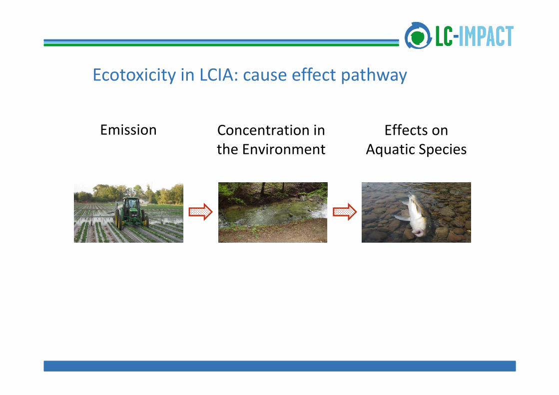
Ecotoxicity in LCIA: cause effect pathway
Emission Concentration in the Environment
Effects on Aquatic Speciesthe Environment Aquatic Species
Ecotoxicity in LCIA: common modeling approach
ConcentrationFractionResidenceEmission e.g. 1 kg/day
Ai• Air Oxidation by OH‐radicals Fast: t1/2 order of hours‐days rate constant: k=ln(2)/t1/21/2 y
• Water
( )/ 1/2
Water Hydrolysis: pH‐dependent Aerobic degradation by bacteria Slower: t days‐weeks Slower: t1/2 days‐weeks
• Soil/sedimentSoil/sediment Aerobic and anaerobic degradation by bacteria Slow: t1/2 order of weeks‐years
Chemical properties: air‐water partitioning
KAW = Cair / Cwater
• KAW = H / RT • H = Vp ∙ Mw / Solp
Vp = Vapor pressurep
Sol = SolubilityMw = Molecular weight
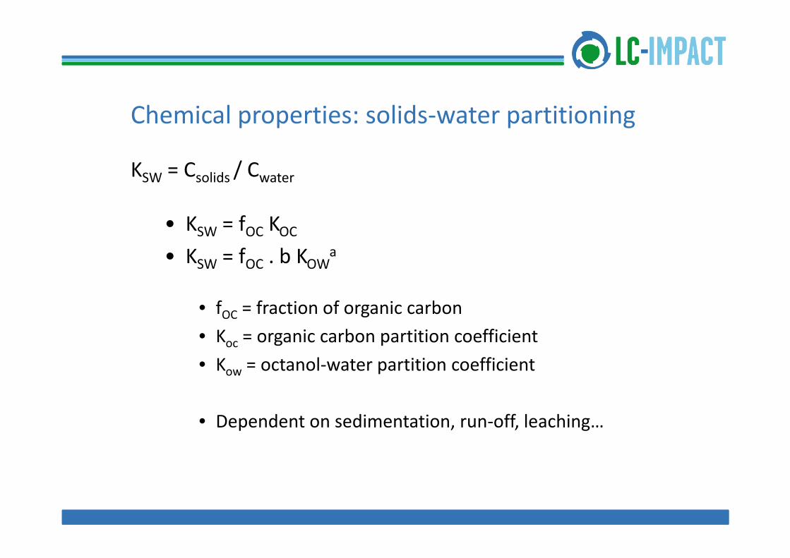
Chemical properties: solids‐water partitioning
KSW = Csolids / Cwater
f• KSW = fOC KOC• KSW = fOC . b KOWa
• fOC = fraction of organic carbon• Koc = organic carbon partition coefficientoc o ga c ca bo pa o coe c e• Kow = octanol‐water partition coefficient
• Dependent on sedimentation, run‐off, leaching…
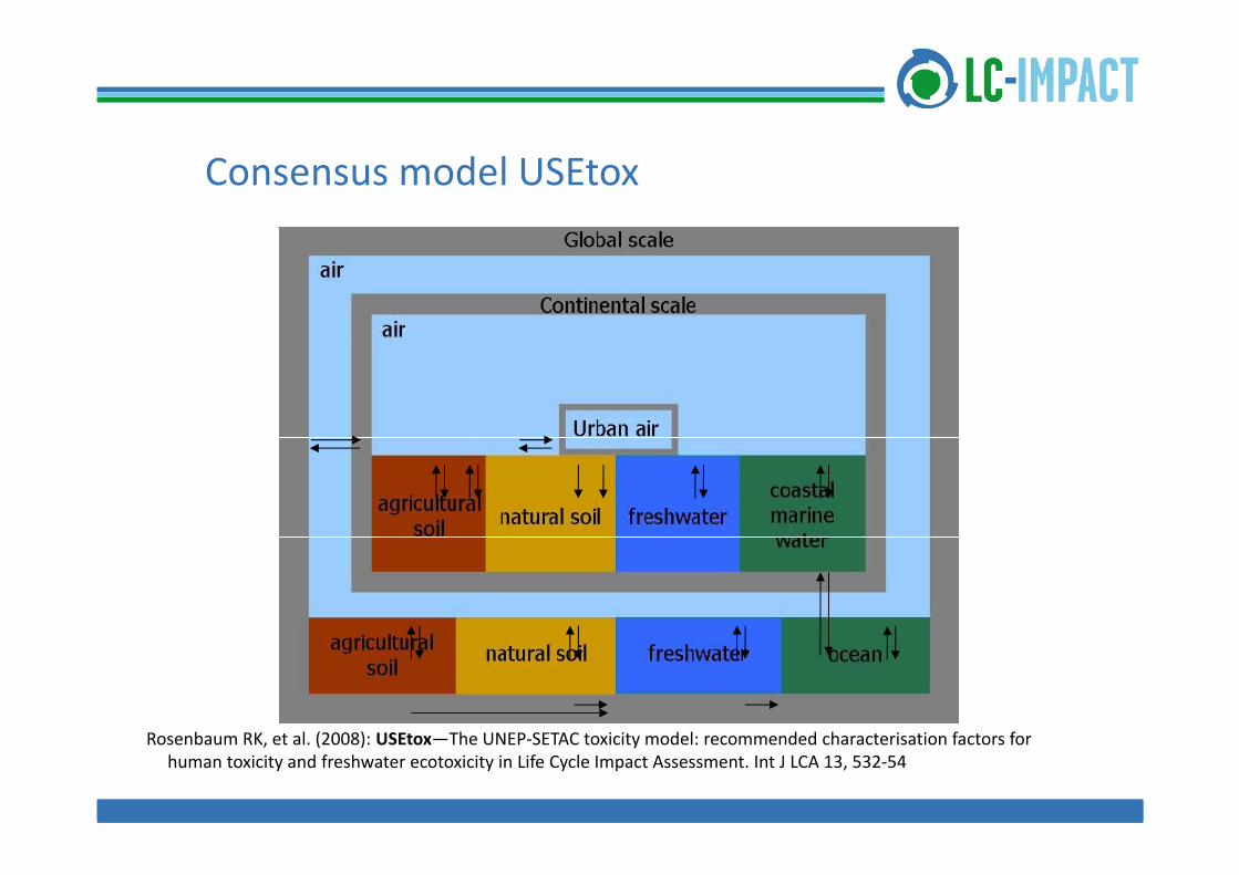
Multimedia fate and exposure model SimpleBox
Den Hollander HA, Van Eijkeren JCH, Van de Meent D (2004): SimpleBox 3.0: multimedia mass balance model for evaluating the fate of chemicals in the environment RIVM Bilthoven The Netherlandsevaluating the fate of chemicals in the environment. RIVM, Bilthoven, The Netherlands
Van Zelm R, Huijbregts MAJ, Van de Meent D (2009): USES‐LCA 2.0: a global nested multi‐media fate, exposure and effects model. Int J LCA 14, 282‐284
Consensus model USEtox
R b RK t l (2008) USEto Th UNEP SETAC t i it d l d d h t i ti f t fRosenbaum RK, et al. (2008): USEtox—The UNEP‐SETAC toxicity model: recommended characterisation factors for human toxicity and freshwater ecotoxicity in Life Cycle Impact Assessment. Int J LCA 13, 532‐54
EXPOSURE FACTOR
22
Exposure factor
• Depends on binding to suspended solids and dissolved organic carbon:
• Exposure of chemical concentration to the ecosystem
XF = dCdis/dCtot = Fdis
dCdis = Dissolved Concentration changedCtot = Total Concentration changedCtot Total Concentration changeFdis = Fraction Dissolved (dimensionless)
BIOACCUMULATION FACTOR
24
Bioaccumulationkx,a,in kx,a,out,a,
kx,w,inkx,f,in
,a,out
kx,w,outkx,f,out
Model: OMEGA (Hendriks et al. 2001)( )
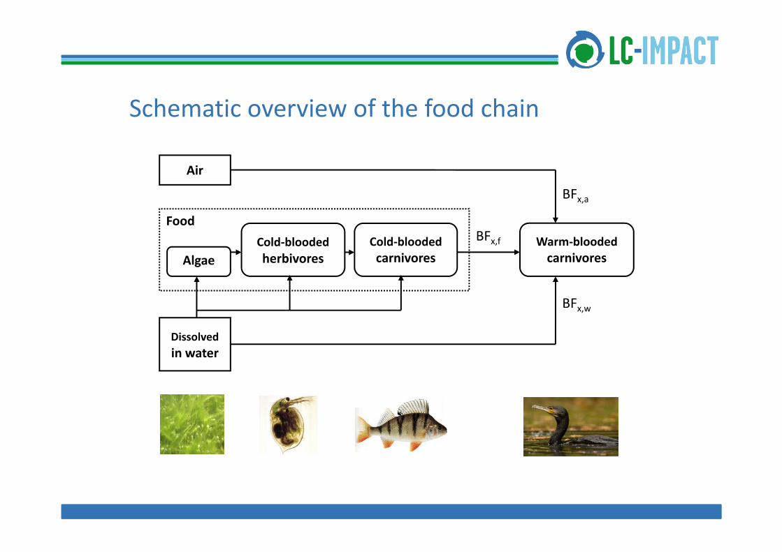
Schematic overview of the food chain
BFx,a
Air
Warm‐bloodedcarnivores
FoodCold‐bloodedherbivoresAlgae
Cold‐bloodedcarnivores
BFx,f
Dissolved
BFx,w
Dissolvedin water
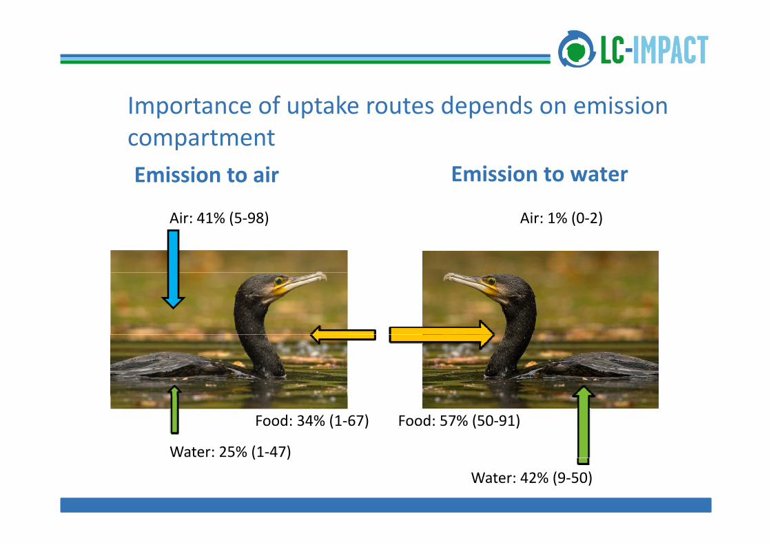
Importance of uptake routes depends on emission compartmentEmission to air Emission to water
p
Air: 41% (5‐98) Air: 1% (0‐2)
Food: 34% (1‐67)
Water: 25% (1‐47)
Food: 57% (50‐91)
( )
Water: 42% (9‐50)
Importance of uptake routes depends on chemical
Lindane (Kow 5.0•103) DDT (Kow 1.55•106)
Water: 2%
Food: 98%Food: 60%
Water: 2%Water: 40%
Summarizing
• Uptake from air is mainly relevant for emissions to air
• Relative uptake from food increased with increasing KowRelative uptake from food increased with increasing Kowat the expense of uptake from water
• For chemicals with a high Kow, uptake from food is by far the most g ow, p yimportant uptake route
3 bioaccumulation factors for warm‐blooded predators
• Bioaccumulation factor for uptake from water
inwxpredatorx kdC
∑ out,x
in,w,x
diss,w,x
predator,xw,x kdC
BF
• Bioaccumulation factor for uptake from food(depends on bioaccumulation in previous trophic levels 1‐3)
BFkdC
∑ out,x
3,xin,f,x
diss,w,x
predator,xf,x k
BFkdCdC
BF
• Bioaccumulation factor for uptake from air
in,a,xpredator,x kdCBF
∑ out,xa,xa,x kdC
BF
EFFECT FACTORS
31
Chemical toxicity to wildlife speciesTh h d d f h i l (HD50) i d i t tThe hazardous dose of a chemical (HD50): upcoming and important
in the toxicity assessment of chemicals for wildlife species
S ll i t l l i → St ti ti l• Small experimental sample size → Statistical uncertainty
• Unrepresenta ve sample of species→ Systematic• Unrepresenta ve sample of species → Systematic uncertainty
• Several ways to enlarge the sample size• Several ways to enlarge the sample size, a.o. interspecies correlation estimation (ICE) models, but these are uncertain
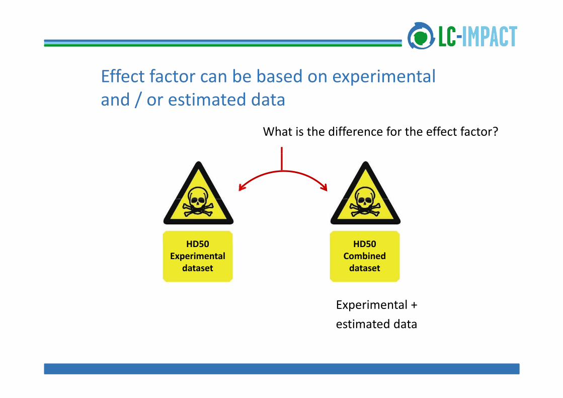
Effect factor can be based on experimental and / or estimated data
What is the difference for the effect factor?
HD50 HD50HD50 Experimental
dataset
HD50 Combineddataset
Experimental + estimated data
Principle of Interspecies Correlation Estimation
R i d t l (2010) id ICE d l t ti t th t i it• Raimondo et al. (2010) provide ICE‐models to estimate the toxicity of 49 wildlife species.
l tiAcute toxicity value of species A
Acute toxicity value of species B
correlation
Acute toxicity value of species C
etc…
• Log (tox. B) = a + b • Log (tox. A) [mg/kgwwt]
Extrapolate toxicity
d d ( )Hazardous dose (HD50): comparing the experimental and combined datasets
Systematic uncertainty typically factor 3.5typically factor 3.5
Hazardous dose (HD50) for mammals only
Birds are more sensitive!
HD50Ex / HD50Co ≈ 1
Birds are more sensitive!
Ex / Co
Calculating the Effect Factor
Limited availability of experimental toxicity data, mainly for mammals → systema c underes ma on of wildlife toxicitywildlife toxicity
Use HD50 values to calculate hazardous body burden:Use HD50‐values to calculate hazardous body burden: HD50 ∙ passimilated
• CFcold‐blooded species >> CFwarm‐blooded species
ff f f• Different ranking of chemicals for warm‐blooded compared
to cold‐blooded species
Best estimate for freshwater impact assessment
• Apply a (weighted) total CF for warm‐blooded and cold‐blooded species to study freshwater impacts– species density– the importance society attributes to protection per trophic level
• Depending on the weighting method, impacts on warm‐blooded predators could change the CFs and relative ranking of toxic p g gchemicals in freshwater impact assessment
Highlights of this presentation
• To estimate the impacts on warm‐blooded species resulting from different uptake routes: insert a bioaccumulation factor
EF)BFXF(FFCF ∑
• The importance of the different uptake routes depends on:
xj
jx,jx,ji,x,ix, EF)BFXF(FFCF ∑
p p pthe emission compartment and the properties of the chemical
• Effect factors can be based on experimental and/or estimated dataLimited availability of experimental toxicity data, mainly for mammals → systema c underes ma on of wildlife toxicity
• CFcold‐blooded species >> CFwarm‐blooded species and the chemical ranking differsImplications depend on the weighting method for the total CF of f h t i tfreshwater impacts
More information?
Golsteijn L, van Zelm R, Veltman K, Musters G, Hendriks AJ,Huijbregts MAJ. 2012. Including ecotoxic impacts on warm‐bloodedpredators in life cycle impact assessment Integr Environ Assess Managpredators in life cycle impact assessment. Integr. Environ. Assess. Manag.8(2):372–378.
Golsteijn L Hendriks HWM van Zelm R Ragas AMJ HuijbregtsGolsteijn L, Hendriks HWM, van Zelm R, Ragas AMJ, HuijbregtsMAJ. 2012. Do interspecies correlation estimations increase the reliabilityof the chemical effect assessment for wildlife? Ecotoxicol. Environ. Saf. 80:238 243238–243.