Income Concentration in a Context of Late Development: An Investigation of Top Incomes in Brazil using Tax Records, 1933–2013 1 Public Policy and Development Master Dissertation Paris School of Economics Marc Morgan Milá 2 Advisor: Thomas Piketty Referee: Facundo Alvaredo This version: 18 September 2015 Abstract This paper presents new estimates on income concentration in Brazil over its development trajectory from 1933 to 2013 using individual tax records. The findings confirm Brazil’s status as one of the world’s most unequal countries, with concentration levels unrivalled elsewhere. Income has been highly concentrated at the top of the distribution, with the top 1 per cent amassing a share of 27 percent in 2013, and consistently fluctuating around 25 per cent since the mid 1970’s. The majority of the income of the very rich in Brazil is not subject to the personal income tax, explaining their low tax liability and the difference between top shares of taxable income and top shares of total income, the latter registering much higher levels of concentration. We also present evidence that household surveys underestimate the extent of income inequality in Brazil. The overall findings illustrate the additional taxable capacity of top income groups, especially in a context where they are not investing as much in the productive capacities of the economy as their share of total income would justify. 1 I thank Thomas Piketty for encouraging me to pursue this project, and for his consistent advice throughout. I am particularly grateful to Facundo Alvaredo, whose meticulous guidance was indispensable for the realization of this project. I also thank Marcelo Medeiros and Pedro Souza for sharing their tax data and their knowledge on many aspects of the Brazilian tax system, and to Roberto Ribeiro for providing the necessary tax statistics for recent years. Finally, my gratitude goes to Naomi Downes for all her moral and sentimental support. All errors are my own. 2 Contact information: [email protected]
Transcript
Income Concentration in a Context of Late Development: An Investigation of Top Incomes
in Brazil using Tax Records, 1933–20131
Public Policy and Development Master Dissertation
Paris School of Economics
Marc Morgan Milá2
Advisor: Thomas Piketty
Referee: Facundo Alvaredo
This version: 18 September 2015
Abstract
This paper presents new estimates on income concentration in Brazil over its development trajectory from 1933 to 2013 using individual tax records. The findings confirm Brazil’s status as one of the world’s most unequal countries, with concentration levels unrivalled elsewhere. Income has been highly concentrated at the top of the distribution, with the top 1 per cent amassing a share of 27 percent in 2013, and consistently fluctuating around 25 per cent since the mid 1970’s. The majority of the income of the very rich in Brazil is not subject to the personal income tax, explaining their low tax liability and the difference between top shares of taxable income and top shares of total income, the latter registering much higher levels of concentration. We also present evidence that household surveys underestimate the extent of income inequality in Brazil. The overall findings illustrate the additional taxable capacity of top income groups, especially in a context where they are not investing as much in the productive capacities of the economy as their share of total income would justify. 1 I thank Thomas Piketty for encouraging me to pursue this project, and for his consistent advice throughout. I am particularly grateful to Facundo Alvaredo, whose meticulous guidance was indispensable for the realization of this project. I also thank Marcelo Medeiros and Pedro Souza for sharing their tax data and their knowledge on many aspects of the Brazilian tax system, and to Roberto Ribeiro for providing the necessary tax statistics for recent years. Finally, my gratitude goes to Naomi Downes for all her moral and sentimental support. All errors are my own. 2 Contact information: [email protected]
Table D.3. Comparison of incomes in tax data and surveys in Brazil, 2008-2012 ................ 164
9
1. Introduction
The research strategy of analysing income inequality on the basis of top income
shares derived from income tax data has received growing impetus since the
publication of numerous individual country studies in the early 2000’s spontaneously
formed a unified and coordinated research project. The output of this research can be
found in the collected series by Atkinson & Piketty (2007, 2010), as well as on the
online website, The World Top Incomes Database, where time series exist for over
thirty countries, across five continents, and spanning long time horizons – often
covering more than 50 years.3 This research is directly inspired from the pioneering
work of Simon Kuznets (1953, 1955), who primarily examined income concentration
in the United States. Contemporary researchers took off where Kuznets left off, by
examining the cases of the most developed OECD countries, namely the France, U.S.
and the U.K., whose relevant fiscal data was readily accessible. But like Kuznets
(1955) before them, these researchers were compelled to study the evolutions of top
incomes in underdeveloped countries wherever data availability made it possible, so
as to be better able to uncover any common or distinct dynamics at play between
distribution and growth in countries at different stages of their development cycle.
Atkinson & Piketty (2010) is a testimony to this effect, including various late
developing countries, such as Argentina, India, China, Indonesia, and Singapore.4
Since then, the Latin American experience has been supplemented by studies on
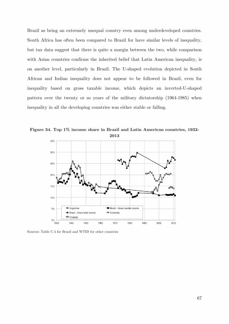
Colombia (Londoño Vélez, 2012) and Uruguay (Burdín et al. 2014); Asia has supplied
by works on Korea (Kim & Kim, 2014), Malaysia (Atkinson, 2015) and Taiwan (Chu
et al. 2015), while South Africa (Alvaredo & Atkinson, 2010) and Tanzania
(Atkinson, 2011) have given representation to the African continent. The present
3 See http://topincomes.parisschoolofeconomics.eu/ 4 See Alvaredo (2010), Banerjee & Piketty (2010), Piketty & Qian (2009), Leigh & Van der Eng (2009) and Atkinson (2010). China’s estimates of top shares are based on household survey data, rather than income tax data, due to the unavailability of the latter.
10
paper follows this line of research by analysing the case of Brazil, a notable absentee
from the above list of late developing countries.5
Investigating income concentration in Brazil can be motivated from numerous
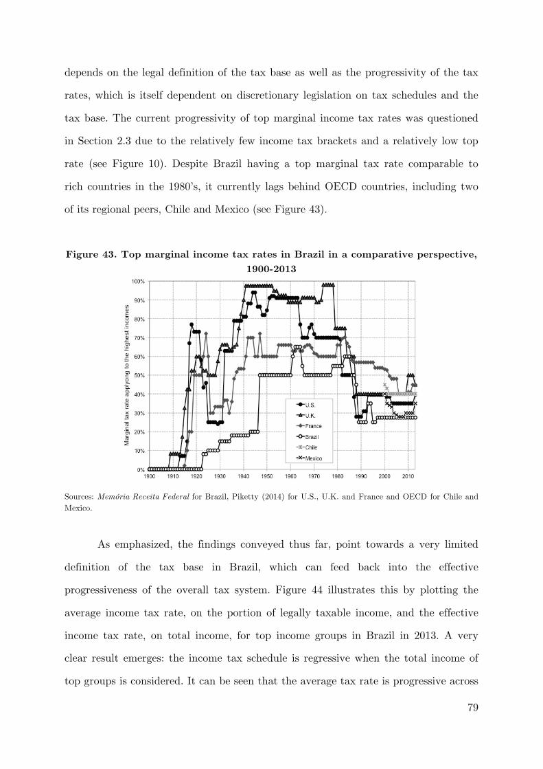
fronts. Firstly, Brazil is part of a region historically characterised by high and
persistent levels of income inequality, since at least the late 19th century (Williamson,
2015). And it is a notable stand-out country of the region - in any report on income
distribution by the OECD, the United Nations or the World Bank, Brazil usually
features near the summit of the inequality rankings, as measured by household
survey data, alongside regional counterparts such as Chile or Colombia. Moreover,
Brazil partakes in the regional characteristic that sources the high inequality in the
disproportionate concentration of income among individuals at the top of the
distribution – individuals at least within the top 10 per cent of income recipients –
rather than in income differences between lower segments of the distribution (Székely
& Hilgert, 1999, Palma, 2011). Given that the studies underpinning these conclusions
are without exception in using data from household surveys, which are prone to
misrepresent the incomes of the very rich, a complementary analysis using income
tax statistics is necessary to evaluate the conventional wisdom.
This necessity is even more pressing when an expansive consensus has
developed, heralding the marked decline in inequality in Latin America since the new
millennium. Brazil has again proven to be an exemplary case study in this context
(López-Calva & Lustig, 2010a). During most of the first decade of the 2000’s it was
the household per capita income of the bottom 10 per cent of families that is reported
to have grown roughly three times faster than the national average (around 2.5 per
cent), while the per capital income of the richest 10 per cent of households
experienced the slowest growth (below average) in the entire distribution, as
measured in household surveys. This apparent decrease in the polarisation of income
5 Medeiros et al. (2015) has been the first attempt to fill this gap for Brazil, in using tax data to evaluate inequality from the top for the recent years 2006-2012.
11
was accompanied by a notable fall in the country’s Gini coefficient from
approximately the average for the previous thirty years of around 0.59 in 2001 to a
historically low level of around 0.55 in 2007 (Barros et al. 2010). This figure
continued to drop over the following six years, reaching, by 2013, a level of about
0.52.6 This is a significant decrease by any standards, which turned Brazil into a
global reference point in the debate on inequality (especially in Western media), with
its flagship conditional cash transfer programs (most notably the Bolsa Familia
program)7, and made Lula da Silva one of the most popular heads of state in the
world.8
This ‘success story’, evidenced from survey-based measures, has been judged
to be due largely to the decline in labour income inequality and non-labour
inequality, rather than to demographic factors or employment prospects of the poor
(Lopez-Calva et al., 2012). It is a narrative that associates the change to a rise of the
bottom of the distribution, rather than any significant decrease of the top. Generally,
the decline in labour income inequality is attributed to a lower skill premium – due
to changes in the composition of supply and demand for labour and to the increase in
the minimum wage raising the earnings of unskilled workers –; a fall in the inequality
of education, and to a lower segmentation of labour markets between rural and urban
workers and between primary and secondary/tertiary workers. This latter factor
could be sourced in the faster growth of some productive sectors in Brazilian
agriculture as opposed to that in more industrial areas (Barros et al., 2010). The
decline in non-labour inequality has been sourced in the expansion in the coverage of
government cash transfers to the poor – such as Benefício de Prestação Continuada,
(a transfer to the elderly and disabled) and Bolsa Família – and an increase in the
6 See SEDLAC (CEDLAS and The World Bank). 7 Starting in 2003 from an amalgamation of previous transfer programs, Bolsa Familia is a means-tested transfer program targeted at poor families that provides cash subsidies for child and mother healthcare and for primary and secondary school enrolment. 8 Lula da Silva’s Workers Party has been in government since 2003; Lula’s mandate lasting between 2003 and 2011.
12
average social security benefit, propelled in part by the increase in the minimum
wage, since some social security benefits, such as non-contributory pensions, are
indexed to the it (ibid).9
It goes without saying that the role of the government in the above narrative
is highly significant, since a large portion of the equalizing forces are reported to
come from either government sponsored cash transfers or government legislation such
as the minimum wage, whose effect seem to be accurately captured in the survey-
based Gini. On the contrary, the contribution of changes in the distribution of
income from capital assets (rents, interests and dividends) is hardly noticeable in the
statistics (ibid). The implication of this is that these income flows may not be
adequately captured in the Gini – their small contribution to overall inequality, and
even to non-labour income inequality, lends weight to the hypothesis that the Gini
measure does not accurately describe what is going on at the top of the distribution.
The absence of the very rich in Brazil from surveys has been a growing
concern, given randomness in the sampling of household surveys and that the capital
assets they are generally dependent upon are either not well measured or are not
observed, due to the reluctance of the richest individuals to disclose all of their
assets.10 Székely & Hilgert (1999) found that Brazil’s principle household survey (the
PNAD) did have relatively good coverage of high incomes for the mid-1990’s, and yet
the majority of the income of the top 10 per cent comprised of labour income from
employees and self-employed workers, similar to the Latin American average.11 But
given what is now known about countries like Colombia, this seems to be a highly
distorted picture. Indeed, the authors point out that their analysis does not exclude 9 Between 2003 and 2013, Brazil’s minimum wage increased by 74 per cent in real terms. 10 Additionally, the rich may refuse to engage in a perceived time-consuming task such as answering a comprehensive household surveys, or statisticians may intentionally remove extreme observations, like those associated to the incomes of very rich, so as to not generate biases in the results. After all, a survey’s primary concern is representativeness, not completeness. 11 This apparent contradiction is due to the authors’ evaluation criteria, by which they compare the income of managers of medium and large firms reported in firm-level surveys to the income of the richest individuals reported in household surveys.
13
the possibility that Latin American inequality is the result of individuals at the top
living off capital income. They are careful in stating that what it does reveal is that
‘the inequality we are able to measure with household surveys in Latin American
countries is informative about a spectrum of society that does not include the richest
households’ (emphasis added). Similarly, in assessing the believed decline in Latin
American inequality since the 2000’s, Lopez-Calva and Lustig (2010b) focus their
analysis on changes in labour income inequality and changes in the size and
distribution of government transfers for the very reason that capital incomes are
underreported in household surveys. 12 The limits of using household surveys to
evaluate the extent of income inequality are thus well understood, and yet belief in
the Brazilian ‘success story’ remains unquestioned. This paper seeks to bridge these
empirical drawbacks by using a novel data source in order to properly evaluate
conventional beliefs concerning inequality in the country.
Brazil is also an interesting case study because it is somewhat of a unique
combination of inequality, size and development. Unlike other similarly judged
unequal countries, like Colombia or South Africa, Brazil is a major economy by
international standards, with the world’s seventh largest GDP.13 From an economic
point of view, Brazil has experienced remarkable transformations since its colonial
period officially ended with the 1891 Constitution proclaiming it a Federal Republic,
with a particularly eventful 20th century. No less dramatic have been its political and
social evolutions.
An early commodity boom, was followed the economic side-effects of World
Wars, and later by an active, state-fomented industrialization program that propelled
the economy onto one of the fastest growth rates observed anywhere during the first
12 They take the observation that an average total monthly household income, of the two richest households in the Brazilian 2006 survey, of $70,357 to be evidence that the incomes of the rich are not captured by the survey. 13 The data currently available for India and China suggest lower levels of inequality, while there is limited data to be able to properly evaluate the case of Russia. The only major economy with comparable levels of inequality at present, one could argue, is the U.S.
14
three quarters of the century, before stagnating structural bottlenecks and into a
developing world debt crisis during the 1980’s, accompanied by mounting
hyperinflation. In between, women were granted the right to vote in the early 1930’s,
which ironically coincided with the autocratic regime of Getúlio Vargas (1930-1945);
a spell of political turmoil in the early 1960’s was followed by a military coup d’état
in 1964, which took over the reins of the country until 1985; while in 1988 universal
suffrage was finally achieved when the literacy requirement for voting was abolished.
Brazil then succumbed to the wave of market liberalisation and financialisation
engulfing developing countries from the early 1990’s, particularly in Latin America.
This culminated in 1994 with the Plano Real, a set of macroeconomic monetary
measures intended to stabilize the economy from runaway inflation, after at least
four failed stabilization attempts (Baer, 2014; Cowell et al., 1998; Engerman &
Sokoloff, 2001; Palma, 2012). The growth performance of this Washington Consensus
period was poor, by historical standards, with the economy slowly contracting, until
the late-1990’s Asian financial crisis brought about a renewed consensus for
developing countries, whereby the role of the state was emphasized in the context of
the Millennium Development Goals, in particular poverty reduction.
From the mid-2000’s, the Brazilian economy entered into another boom phase
– mostly led by commodities, but also by finance and household credit, particularly
for real estate – which was only mildly halted by the global economic crisis of 2008-
2009 (Palma, 2012). Figure 1 summarizes Brazil’s economic performance. Although
the proceeds of Brazil’s recent growth spurt – a pale comparison to its ‘golden age’ of
import-substitution growth (1955-1980) – succeeded in reducing poverty, its impact
on the market distribution of income remain in question, due to the shortcomings of
the traditionally used data. Given the sources of this growth, it is unlikely that much
of its benefits initially reached the middle and lower groups of the distribution.
Indeed, the initial findings by Medeiros et al. (2015) seem to confirm that a
disproportionate share of income flowed to the very summit of the distribution (the
15
top 1 per cent and beyond) during the period 2006-2012. It is therefore interesting
and necessary to examine income concentration in Brazil throughout its tumultuous
recent and past history to re-evaluate the link between income distribution and
economic development.
Figure 1. Average real income and consumer price index in Brazil, 1930-2014
Source: Table B.3.
Finally, there exist few studies that track the long-run evolution of inequality
in Brazil, over a time frame longer than twenty-five years. One reason for this
timeframe is that it generally coincides with the availability of household survey data
(for example, see Ferreira et al. (2007)). Prior to the 1980’s, approximations of the
distribution of income have relied upon single year estimates, coinciding with the
availability of decennial Census data. Thus, the earliest studies of any empirical
rigour to examine inequality in Brazil have been for the years 1960 and 1970 (see for
instance, Langoni (1973) and Fishlow (1972), both of whom report an increase in net
income concentration among the top percentiles over the decade). Hence, the present
paper is the first attempt to present a long-run quantified history of income
16
concentration for Brazil, and one of the few for a country of Latin America.14
Furthermore, the present study takes a novel stance by exclusively focusing on gross
market income inequality. Most of the existing research on Brazil examines
disposable income inequality, that is, the inequality of income net of direct taxation
and transfers. This is a significant departure, firstly because the pre-tax distribution
of income may offer different conclusions to the after-tax distribution of income, and
secondly, because the latter is heavily dependent on the former, in its capacity for
redistribution. 15 And also, the development path of a country can be both a
consequence and a cause of the existing pre-tax distribution of income. An
exploration of income tax records can thus contribute to provide a more complete
picture of the actually existing state of income distribution in Brazil.16
As well as being informative about distributional skewness in society, studying
the evolution of top income shares in general is important for other reasons. As
previously highlighted, the development path of a country, as well as the means the
country affords towards it, can be heavily influenced by the portion of a country’s
income that is concentrated in few hands (and visa-versa) since affluent groups have
property rights over resources and thus can impact the country’s growth trajectory.
From a policy perspective, top income shares may reveal something more than just
the state of inequality. Also, given the value of income captured in top income
shares, these can affect more broad measures of inequality, like the Gini coefficient,
at the national and global level (Atkinson, 2007). Brazil’s recent ‘success story’ is
14 Alvaredo (2010) is the only other study that examines the evolution of a Latin American country starting before the 1990’s, covering a total of 38 years over a 72-year period. The present study, on the other hand, covers a total of 62 years over an 80-year period. 15 Paraphrasing José Palma, it’s the original share of income of the rich that really matters, as the rest of the population follows suit (see Palma, 2011). 16 For example the finding by Fereirra et al. (2010) that inequality in Brazil remained stable during the market liberalization period of the early 1990’s, contrary to other Latin American countries, just reveals the partial nature of looking at the net income distribution using survey data. A study of the original market distribution of income may throw up different conclusions, and offer new perspectives for the analysis of income inequality.
17
marked by a sustained fall in the recorded Gini, but uncovering top income shares
may suffice to alter the final conclusion. Finally, and from an ethical point of view,
social beliefs about what characterises a fair distribution of income can influence
political economy responses such as redistributive taxation. And these beliefs can
strongly be informed by investigations made public on income concentration in a
particular society.
Recent research on the topic has found that for most countries surveyed, top
income shares have followed one of two patterns since the beginning of the 20th
century (when most income tax systems were founded). There is a group of ‘U-
shaped’ countries (Anglo-Saxon countries and developing countries like Argentina,
India and South Africa), characterised by very high income concentration at the
beginning of the century, a large plunge in shares during the middle thirty years of
the century, and a rapid rise in inequality since the 1980’s reaching the levels
observed at the beginning of the 20th century in the new 21st century. And there is a
group of ‘L-shaped’ countries (continental Europe, Japan and neighbouring middle-
income Asian countries), characterised by high levels of concentration early on in the
century, a downward swing over the mid-century, followed by a mild rise, if not
quasi-stable evolution, from the 1980’s until the present (see Atkinson et al., 2011).17
To see how Brazil compares to these evolutions is one of this paper’s main research
questions.
Nevertheless, the use of tax data is not without some shortcomings of its own.
First, the tax-paying population strictly determines the portion of the income
distribution (and thus income shares) that can be studied. In developing countries
like Brazil, these may account for a relatively small number of people, especially in
earlier years. Indeed the picture we get for Brazil is that for much of the century,
only a small minority of the total population provided information to the tax
17 See also the World Top Incomes Database for up-to-date country information.
18
authorities, as Section 2 will document. This technical detail means that for the most
part, the conclusions drawn from the data are silent on the distribution of income
outside of the top groups, namely within the bottom 90 per cent of the population.
As mentioned, the estimates are also silent on post-tax and transfer income. They
deal mostly with the distribution of taxable income, rather than national income, so
the tax definition of income generally falls short of the definition ideally applied,
which means that the estimates produced from the data are somewhat under-stated.
Furthermore, tax data usually miss tax-exempt income, and can never capture tax
evasion, by definition. Fortunately, the Brazilian tax data does capture tax-exempt
and non-taxable income for a certain number of years, as shall be exposed below. In
any case, the description of the underlying distribution of income provided by tax
data must be seen as partial and thus complementary to equally partial alternative
sources such as household surveys. Yet despite the aforementioned drawbacks of tax
data, they remain the most informative source to study the extent to which the
original distribution of income is concentrated, and whether this concentration
accentuates or weakens over time.
This study obtains five main results. First, income in Brazil is highly
concentrated, given that the top 1 per cent of the distribution accounts for about 27
per cent of total gross household income in 2013. Top income shares in Brazil are the
highest observed in the whole WTID sample for recent years, as well as historically,
since top shares reached higher peaks during the caotic 1980’s. On the basis of these
results, Brazil is more unequal than any of its developing country peers, and the
United States, even after accounting for capital gains in the latter. Only the top 0.01
per cent in the U.S. can compare to its equivalent in Brasil over recent years.
Moreover, these high shares appear to be a persistent feature of Brazil’s development,
as they have changed little since the 1970’s, dampening the enthusiasm over Brazil’s
‘success story’.
19
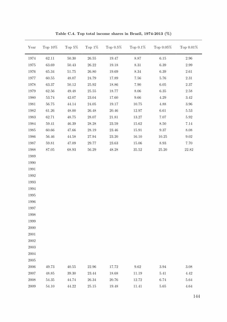
Second, the distribution when measured from taxable income presents a
markedly different picture than the distribution when measured from total income.
Taxable income shares are consistently much lower than the total income shares, for
which we have less data. According to gross taxable income, top income shares have
maintained a constant trend since the late 1980’s, with the top 1 per cent share being
in the order of 11-12 per cent, more than half what shares according to total income
reveal for the recent years. Historically, the gross taxable shares have fluctuated more
considerably than the total income shares, with an evolution comparable to the
shares of total income in a country like Argentina.
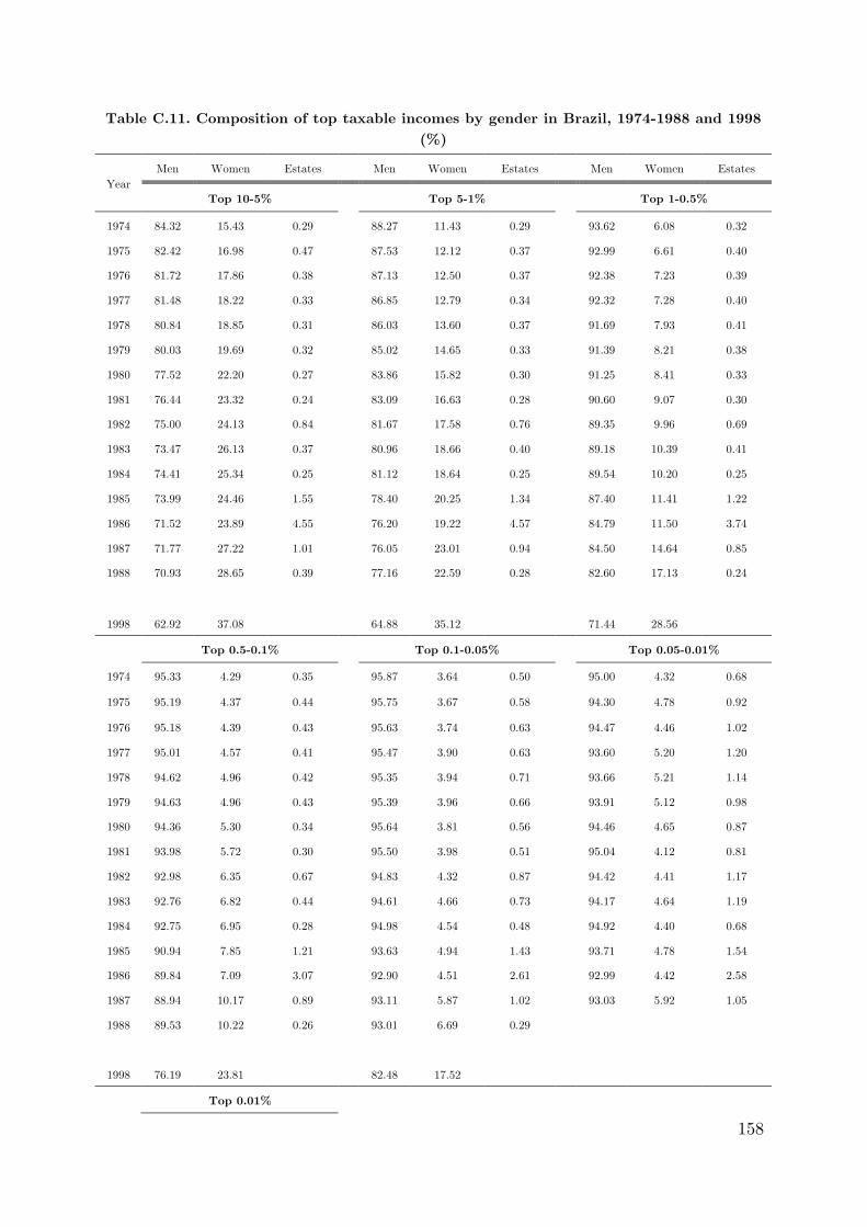
Third, the compositions of taxable incomes during the 1970’s and 1980’s reveal
that top groups in Brazil obtained the bulk of their income from wages. At first
glance this appears at odds with the pattern found in most developing countries,
where it has been found that the rich are primarily capital owners. However, given
the difference in taxable incomes and total incomes at the top, it is likely that the
compositions are highly distorted. This not so much the case for the compositon of
top incomes by gender, where it is more likely that the greater representation of
women reflects real social changes between the late 1970’s and the late 1990’s.
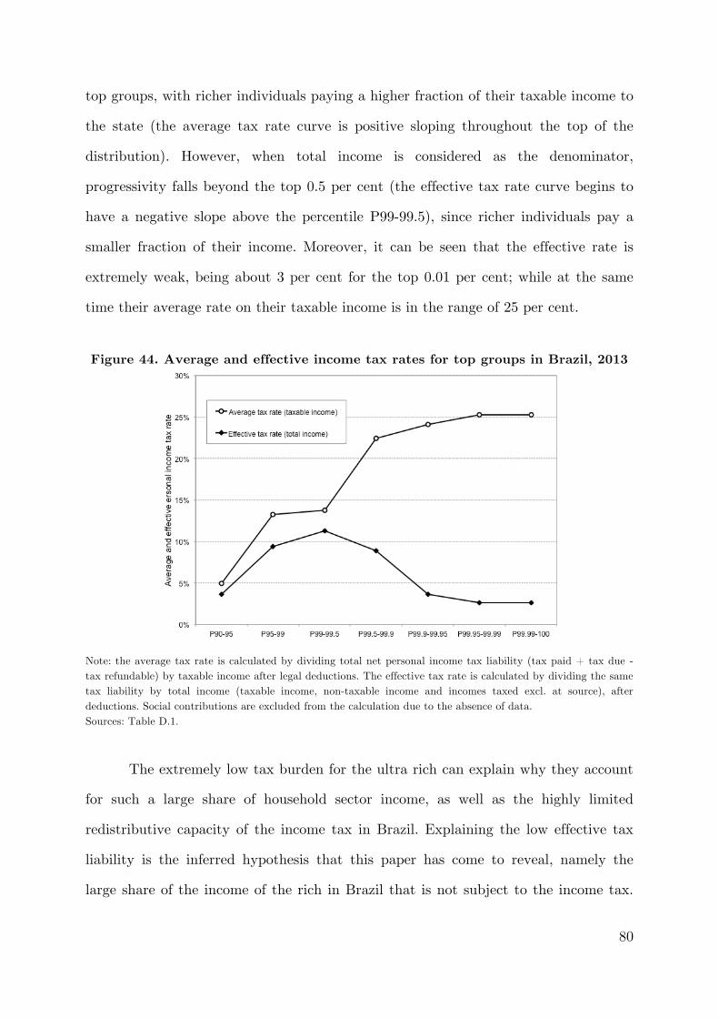
Fourth, the relative tax burden of top income groups reveals the differences
between the taxable income distribution and the total income distribution. The
current effective tax rates paid by the upper part of the distribution are extremely
low (3-4 per cent), and can be explained by the tax reliefs associated the most
important sources of capital incomes – profits and dividends.
Fifth, preliminary comparisons with existing estimates of income concentration
based on household surveys reveal a potential underestimation of inequality on behalf
of survey-based estimates. These estimates, while close in level to the taxable income
shares from tax data, are far from what the shares of total income report.
From a purely qualitative perspective, these results do not say anything new
about about income distribution and tax systems, in a region cited for high inequality
20
and tax evasion. Nevertheless, they provide an additional lense, through which
distributive questions can be examined. And the results reveal the extent to which
concerns over tax evasion may be overstated, given the low incentives to evade
already soft tax systems. Nevertheless, as with any study using tax data, our
estimates should be taken with all the methodological caveats in mind.
The remainder of the paper is structured as follows. Section 2 offers some
background on the fiscal context in Brazil, particularly from a taxation point of view.
Section 3 describes the data and methods used to arrive at the results. Section 4
presents the findings surrounding top income shares over the long run, conveys some
compositions of income, and places the general results in an international perspective.
Section 5 discusses the measurement, interpretation and implications of the findings.
Section 6 concludes with some guidelines for future research.
2. Fiscal context: development and taxation in Brazil
2.1 The rise of the Brazilian fiscal-social state The interwar period in Brazil was marked by growing investment, rapid growth in
industrial production and early attempts at collective planning, especially in the
1930’s. Active industrialization policies did not commence until after 1945 (Baer,
2014). Brazil was in a context of late development. From the mid-1920’s, there was
also a notable shift in the country’s public finances. This was spurred on the one
hand by growing tax revenues from industrial production and by the creation of the
federal income tax in December 1922, despite previous efforts by public officials to
institute it, at the end of the monarchical empire in the late-19th century and at the
beginning of the Republic in the early 20th century (Da Nóbrega, 2014). On the other
hand, there was an expansion of public expenditures, notably the emergence of social
assistance and social security spending at the federal level the same year as the
21
income tax came into effect. This new form of social spending added to that already
undertaken in the domains of education and healthcare by all tiers of government.
Despite Brazil’s chaotic political history, the country was able to develop a
remarkably large fiscal-social state by comparative international standards. Figure 2
testifies this, showing Brazil to have a current level of public social expenditures
comparable to the OECD average, well above its regional neighbours Chile and
Mexico, and greater than that of countries like the U.S.18 A look at some orders of
magnitude surrounding Brazil’s tax revenues reveals an equally impressive evolution,
which have no doubt facilitated the large rise in the country’s social expenditure.
Figure 2. Evolution of public social transfers in Brazil in a comparative
perspective, 1930-2013
Note: public social transfers for the purposes of this comparison excludes spending on housing, as well as education, in order to maintain consistency with the measure for other countries. Sources: Author’s calculation for Brazil using data from IBGE and from the Ministério de Fazenda. Data for other countries is from Lindert (1992 and 1993) for 1930-1981 and from OECD SOCX for 1982-2013.
18 In fact, one could argue that Brazil was always ahead of its time, since it committed a greater share of its economy to public social transfers than what developed countries spent in their earlier histories at similar levels of economic development, for instance, by comparing Brazil around 1975 with both Sweden or France around 1930, or Brazil in 2013 with France around 1960 (taking 1990 US dollars PPP as the reference, see The Maddison-Project at http://www.ggdc.net/maddison/maddison- project/home.htm). Including spending on education, housing and urban services and labour increases the social spending share in GDP by 5-7 percentage points for recent years (see Figure E.1 in Appendix). Brazil’s total primary public spending has increased from an average of about 15 per cent of GDP between 1900 and 1945 to over 45 per cent of GDP today (see Figure E.2 in Appendix).
22
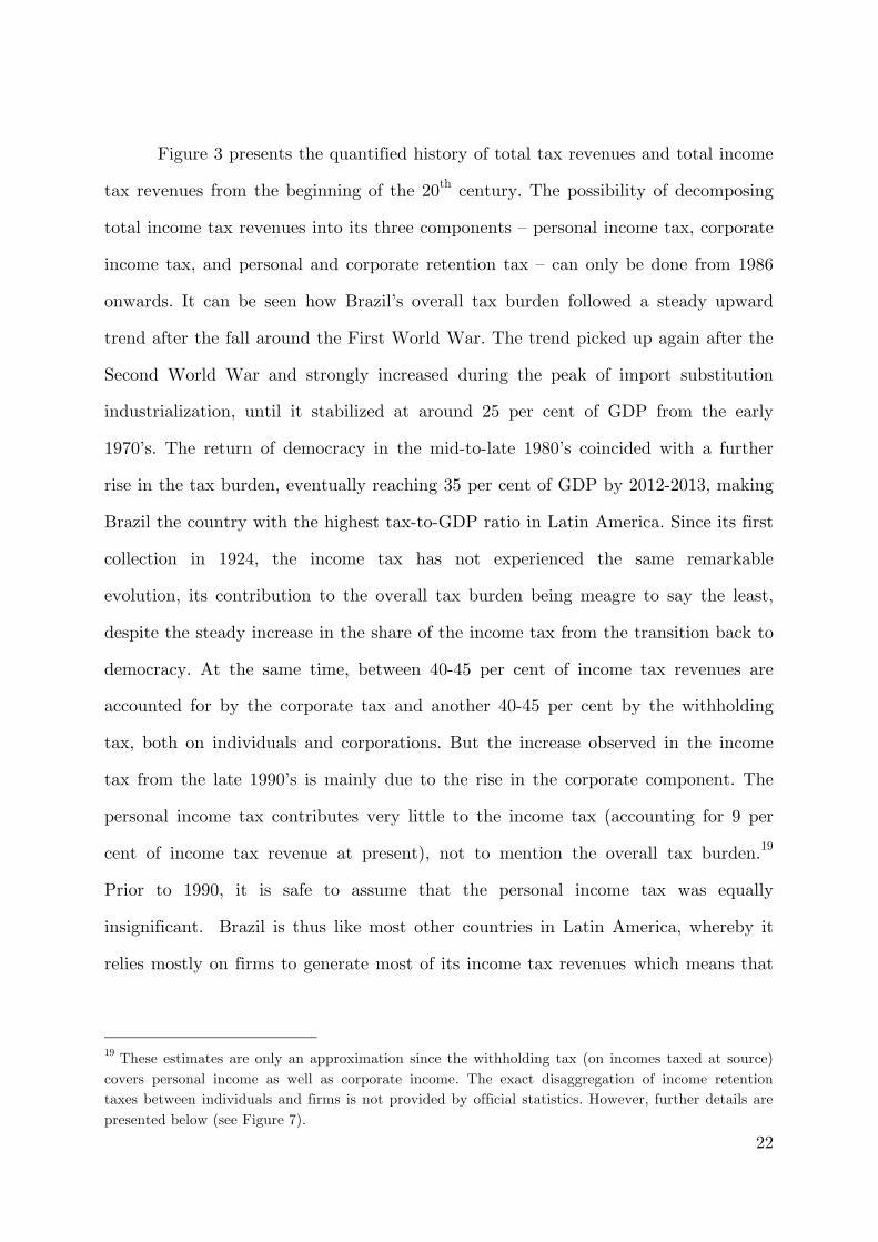
Figure 3 presents the quantified history of total tax revenues and total income
tax revenues from the beginning of the 20th century. The possibility of decomposing
total income tax revenues into its three components – personal income tax, corporate
income tax, and personal and corporate retention tax – can only be done from 1986
onwards. It can be seen how Brazil’s overall tax burden followed a steady upward
trend after the fall around the First World War. The trend picked up again after the
Second World War and strongly increased during the peak of import substitution
industrialization, until it stabilized at around 25 per cent of GDP from the early
1970’s. The return of democracy in the mid-to-late 1980’s coincided with a further
rise in the tax burden, eventually reaching 35 per cent of GDP by 2012-2013, making
Brazil the country with the highest tax-to-GDP ratio in Latin America. Since its first
collection in 1924, the income tax has not experienced the same remarkable
evolution, its contribution to the overall tax burden being meagre to say the least,
despite the steady increase in the share of the income tax from the transition back to
democracy. At the same time, between 40-45 per cent of income tax revenues are
accounted for by the corporate tax and another 40-45 per cent by the withholding
tax, both on individuals and corporations. But the increase observed in the income
tax from the late 1990’s is mainly due to the rise in the corporate component. The
personal income tax contributes very little to the income tax (accounting for 9 per
cent of income tax revenue at present), not to mention the overall tax burden.19
Prior to 1990, it is safe to assume that the personal income tax was equally
insignificant. Brazil is thus like most other countries in Latin America, whereby it
relies mostly on firms to generate most of its income tax revenues which means that
19 These estimates are only an approximation since the withholding tax (on incomes taxed at source) covers personal income as well as corporate income. The exact disaggregation of income retention taxes between individuals and firms is not provided by official statistics. However, further details are presented below (see Figure 7).
23
the progressive objectives of the personal income tax remain to be exploited
(Cetrangolo & Gomez-Sabaini, 2007).
Figure 3. Evolution of total tax revenue and income tax revenue in Brazil, 1900-2013
Sources: Author’s calculation using data from IBGE and from the Ministério de Fazenda.
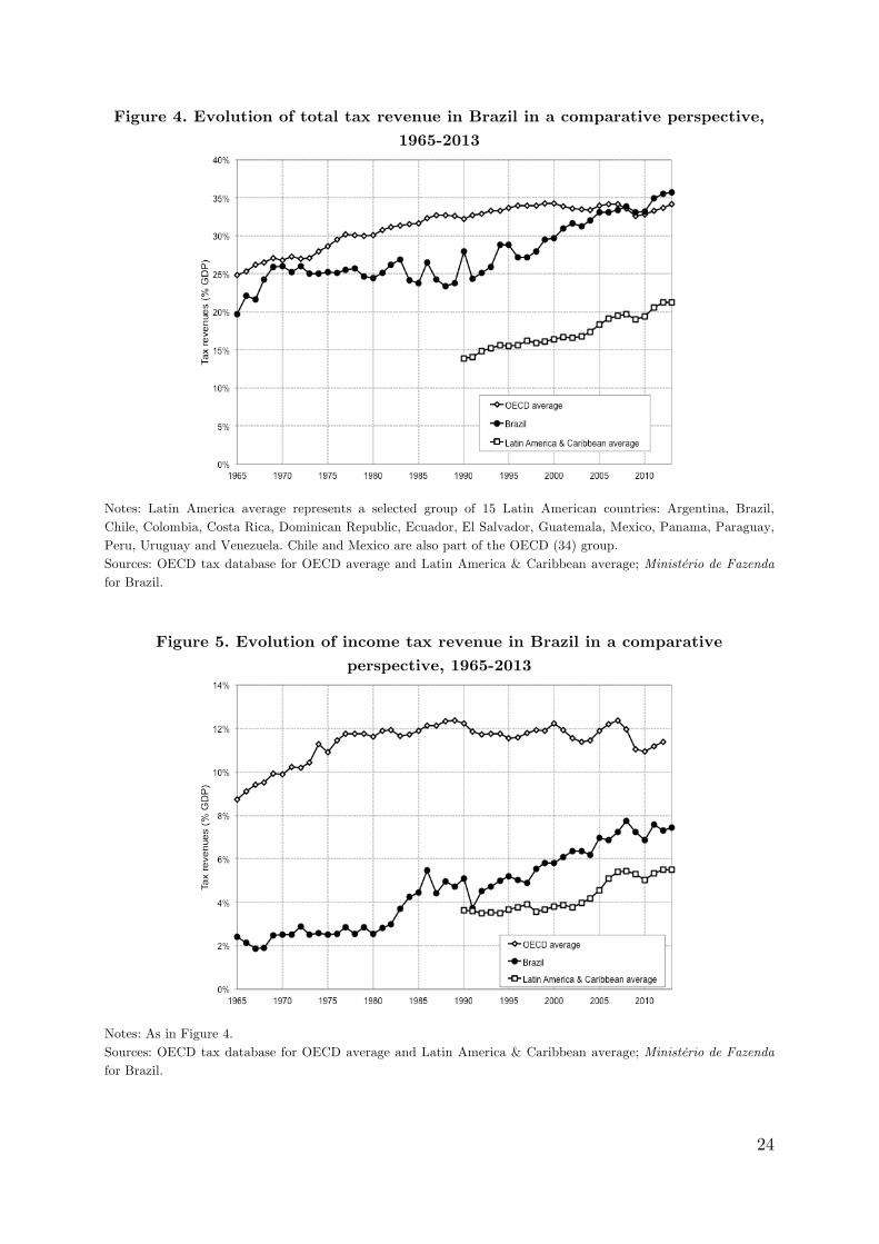
While Brazil appears to be a standout country in Latin America regarding its
overall tax revenues, ranking close to the average OECD country, the opposite is true
concerning its relative income tax burden. Figure 4 and Figure 5 depict these facts
more clearly. The weak contribution of the Brazilian income tax to total tax
revenues, as conveyed in Figure 3, is quite characteristic of Latin American countries
in general, as Figure 5 coveys, despite Brazil having OECD tax-burden-levels in
recent years (see Figure 4). As mentioned, it is likely that the relatively high tax
collection in Brazil has facilitated the redistributive programs on the expenditure side
that have caught the eyes of many observers since the 2000’s.
24
Figure 4. Evolution of total tax revenue in Brazil in a comparative perspective, 1965-2013
Notes: Latin America average represents a selected group of 15 Latin American countries: Argentina, Brazil, Chile, Colombia, Costa Rica, Dominican Republic, Ecuador, El Salvador, Guatemala, Mexico, Panama, Paraguay, Peru, Uruguay and Venezuela. Chile and Mexico are also part of the OECD (34) group. Sources: OECD tax database for OECD average and Latin America & Caribbean average; Ministério de Fazenda for Brazil.
Figure 5. Evolution of income tax revenue in Brazil in a comparative perspective, 1965-2013
Notes: As in Figure 4. Sources: OECD tax database for OECD average and Latin America & Caribbean average; Ministério de Fazenda for Brazil.
25
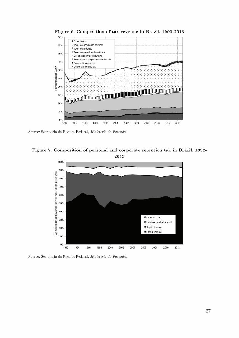
2.2 The composition of tax revenue If the income tax contributes so little to overall tax revenue, from which tax
categories is the large tax burden sourced? Unfortunately, the answer to such a
question can only focus on the years since 1990, due to data availability. However,
this is in an interesting period given that it coincides with a sharp and sustained
increase in the tax burden, as seen from Figure 3. The structure of tax revenue is
presented in Figure 6 for the period 1990-2013. It can be seen that the relative
magnitudes of the different taxes have not changed much over the 23 years.
Social security contributions have increased their share in total tax revenue,
but remain the second largest tax category, in terms of revenue generation
(accounting for just under 10 per cent of GDP in recent years). Representative of
Latin American countries is Brazil’s heavy reliance on indirect taxation, particular
taxes on ordinary goods and services, which on their own have made up between 14
and 15 per cent GDP since the early 2000s. This compares approximately to 12 per
cent of GDP in Argentina in 2004 (Alvaredo, 2010) and to around 9 per cent of
national income in Colombia in 2009 (Londoño Vélez, 2012). Value-added taxes, like
in many other countries in the region, make up the majority of the revenue in this
category (OECD/ECLAC/CIAT/IDB, 2015). A further popular tax in Latin America
is the property tax, although its burden is not very high at around 2 per cent of
GDP, much like in other countries of the region. In Brazil, this tax is made up of
recurrent taxes on immovable property (around 25 per cent of the total), which are
almost entirely from the tax on urban land property; estate and inheritance taxes
(around 5 per cent), taxes on financial and capital transactions (around 40 per cent),
and other recurrent property taxes (around 30 per cent). Although much talked
about, Brazil has never instituted a recurrent tax on net wealth, on either individuals
or corporations.
As was previously discussed, taxes on income and profits seem to be skewed
somewhat towards corporations. However, some qualifications may be needed, given
26
that the withholding tax combines both the individual and corporate spheres. Figure
7 depicts the composition of this tax among identifiable sources. It can be seen that
between 50 and 60 per cent of the tax comprises of labour income, which is
attributable to the personal income tax. The remaining proportions are composed of
income from both individuals and firms, so it is unclear as to the definitive split
between the two in the income tax.
Regarding the composition of tax revenues in earlier parts of the century,
official statistical publications allow us to get some idea of the relative importance of
different taxes, mostly at the federal level, which has historically concentrated around
70 per cent of total tax revenues. Until the First World War, trade taxes were the
principle source of revenue in Brazil, with tariffs accounting for almost 80 per cent of
the federal government’s principle receipts (and almost 8 per cent of GDP). The
reductions in global trade flows brought about by the War lead to a drastic decline in
the importance of tariffs to the Brazilian economy – during the 1920’s and 1930 the
share of tariffs in GDP was more than halved. During the 1940’s, they lost their
primary hold over the economy to consumption taxes, particularly the tax on
industrial products, and to the income tax. During the 1950’s and 1960’s, the tax on
industrial products continued to increase, reflecting Brazil’s growing industrialization
process, until it reached its peak in the early 1970’s (representing nearly 5 per cent of
GDP). From the late 1970’s, it was definitively replaced by the income tax as the
main source of tax revenue for the federal government (IBGE, 2006).
27
Figure 6. Composition of tax revenue in Brazil, 1990-2013
Source: Secretaria da Receita Federal, Ministério da Fazenda.
Figure 7. Composition of personal and corporate retention tax in Brazil, 1992-2013
Source: Secretaria da Receita Federal, Ministério da Fazenda.
28
2.3 The personal income tax The distance travelled by Brazil’s tax revenue over the previous 80 years is
impressive to say the least. Yet it may seem puzzling that the income tax,
particularly the personal income tax, has remained so stable over the period when the
average real income per adult has made remarkable gains, as Figure 1 attests.
However, these twin evolutions can be better understood if we take into account the
tax reliefs and the large initial exempted income bracket that have characterised the
personal income tax since its creation.
As mentioned above, the modern personal income tax in Brazil first came into
effect in 1923, after a number of previously failed attempts dating from the mid-19th
century. Between the mid-1920’s to the mid-1960’s, the tax payable was calculated in
the following manner: gross personal revenue and deductions were divided into
different income schedules, with a proportional tax levied on the gross income (after
deductions) per schedule at different rates.20 A progressive tax was then imposed on
total net income, after allowances (abatimentos) were subtracted. In 1965, the
proportional tax was abandoned by the military regime, while the schedular system
was abolished in 1990, after the country had returned to democracy (Da Nóbrega,
2014).21 Thus, the tax relief applicable during the first period included schedular
deductions, primarily for expenses incurred to generate the income flow in each
schedule, and allowances for social expenditures not related to expenses incurred to
generate the income reported for tax. Over time these allowances have included items
like interest on personal debt, life insurance premiums, personal medical expenses,
educational expenses, contributions to social security funds, rent, alimony, expenses
20 I employ the different terms ‘gross revenue’ and ‘gross income’ to best approximate their respective translated counterparts in the publications, ‘rendimento bruto’ and ‘renda bruta’. The schedules represent different income categories, by which taxpayers could divide the total income they earned into its different sources on the tax form, such as capital income (interests, dividends), property income (rent), salaried work, self employment, agricultural income, etc. See Appendix A for more details. 21 See Appendix A for details on the calculation of the income tax along its evolution.
29
on dependents, among other expenses. Further tax relief was granted to individuals
making stock investments between the late 1960’s and the early 1990’s (ibid). When
the schedular system was abolished in the early 1990’s, the allowances remained the
only deductible items possible on income tax forms. 22 In recent years, these
deductions comprised mainly of expenditure on dependents (spouse, children, parents
etc.), contributions to public and private social security funds, limited educational
expenses for the tax filer and their dependents, medical expenses, alimony (spousal
maintenance expenses), the standard discount (desconto padrão) for salaries and
deductions for intermediate consumption of contributors receiving income from non-
salaried work (Livro Caixa).
Moreover, since its creation, the personal income tax has not had wide
coverage, with certain income sources being either exempt from the tax or taxed
exclusively at source, often at lower rates (ibid). Over the years, the relative scope of
non-taxable incomes increased, especially between the 1970’s and 1980’s. The large
majority of the total income of top income groups, at least since the 1970’s, has
comprised of non-taxable income and incomes taxed exclusively at source, as shall be
revealed below. It is no wonder then that at present, capital gains are taxed
exclusively at source, while dividends and profits are non-taxable sources of income,
fully exempt from the income tax.23
The second feature of the personal income tax partly explaining the low
collected revenues are the relatively high exemption levels on the tax. Figure 8
presents the ratio between the exemption limit and the average income per tax unit.
22 Between 1976 and 1989 a standard deduction (desconto padrão) of about 25 per cent also applied to gross personal revenues from salaried work (up to a pre-defined threshold), which replaced all schedular deductions and allowances for those claiming it, with certain exceptions for allowances (generally costs of rent, family care and medical/hospitalization costs). This measure was intended to promote formal employment. This discount was recovered in the tax year 1996 (after it had been repealed during the tax reforms of the early 1990’s) at a rate of around 20 per cent, again up to a pre-determined threshold (Da Nóbrega, 2014). 23 See Tables A.1 and A.2 in the Appendix for a list of the income categories taxed exclusively/definitively and those considered exempt/nontaxable in 2013.
30
It can be seen that despite the clear downward trend, the exemption limit remains
close to average incomes. Hence, the low personal income tax revenues for the early
part of the century can be understood to be mainly the result of extortionately high
exemption levels, where only a tiny minority paid the tax. Indeed, Figure 9 depicts
that, for the first 45 years of the tax, no more than 1 per cent of the total number of
potential taxpayers were a contributor. However as the exemption limit grew
relatively less than average incomes, especially from the 1970’s, it is likely that the
tax reliefs played a more important role in determining the low collection rates since.
Figure 9 also displays that the total number of tax returns as a percentage of the
potential taxpaying population increased markedly since the founding of the Federal
Tax Office (Receita Federal do Brasil) in 1968. After an initial sharp rise in the early
1970’s the proportion of taxable tax units hovered around 13 per cent since the mid
1970’s to the late 1990’s, after which it rose to reach over 20 per cent by 2007 – a
threshold it has since maintained.24
The marginal tax rates and associated brackets have also experienced dramatic
evolutions throughout lifespan of the personal income tax. Figure 10 summarizes the
quantified history of the top marginal tax rate and the basic rate after the exemption
threshold. The top marginal rate rose sharply after the Second World War, reaching
its peak of 65 per cent during the short term of João Goulart’s left-wing government.
It remained at or above 50 per cent through the twenty-year dictatorship until the
late 1980’s transition back to democracy, when the rate was practically halved. The
current rate of 27.5 per cent has been untouched since 1997, despite the Workers
24 The sharp spike observed over the late 1960’s/early 1970’s is explained by the large increase in the number of tax returns. The number increased tenfold from 1967 to 1968, and then doubled from 1968 to 1970. This can be attributed to the decline in the exempted tax threshold for salaried income, which declined by a factor of around ten between 1967 and 1968, and continued to decline for the following few years. The marked decline in the proportion of taxable tax units between income year 1974 and income year 1975 again relates to the decline in the number of tax returns. This corresponded to a modification in the tax law, whereby the exemption threshold increased between 1974 and 1975, applying to total income 1974, while applying for taxable income only from 1975 (Da Nóbrega, 2014).
31
Party being in power since 2003. This development almost mirrors that in the
developed countries, leading to the hypothesis that Brazil’s taxation was responding
to international trends rather than changes in the domestic political arena. On the
other hand, the lowest marginal tax rate has experienced a continuous upward trend
roughly until the recent global financial crisis of 2008-2009.
Figure 8. Exempted income tax threshold as a fraction of average income per tax unit in Brazil, 1930-2013
Source: Table B.3. Coloumn [8].
Figure 9. Proportion of taxable income tax units in Brazil, 1933-2013
Source: Table B.2. Coloumn [8].
32
A similar narrative applies to the evolution of the number of tax brackets
(Figure 11). Since the early 1990’s the number of tax brackets has fluctuated between
two and four ranges, compared to an average of about twelve for the previous 70
years. For much of this period there were only 10 percentage points separating the
top marginal rate from the lowest rate, when only the two rates existed. The
implications for the progressiveness of the personal income tax and for the pure
redistributive objectives of the tax were thus extremely bleak. Since the crisis there
has been a slight improvement, as two more tax brackets have been introduced, and
the lowest rate has been decreased.
Figure 10. Top and basic marginal tax rates in Brazil, 1923-2013
Source: Memória Receita Federal.
33
Figure 11. Number of personal income tax brackets in Brazil,1923-2013
Source: Memória Receita Federal.
3. Data and methodology
3.1 Data sources, data coverage and income concepts The complete series for the shares of income appropriated by top income groups
stretches between 1933 and 2013 intermittently due to missing data for some years
and to the separate series produced for shares calculated on the basis of taxable
income and for shares calculated on the basis total income (taxable income, non-
taxable/exempt income and incomes tax exclusively at source), the latter only
available for a limited number of years. The basic data sources used in this paper to
estimate top shares comprise exclusively of income tax tabulations based on the
universe of tax filers, reporting by ranges of pre-tax income, the total number of tax
filers and total income in each bracket over the entire period 1933-2013. Other
variables in the tax returns, such as income source, gender, and the decade of birth of
tax filers are available between the years 1969 and 1988, but concern taxable incomes
only.
34
The data between 1933 and 1960 come from historical publications of Brazil’s
national statistics institute, the Instituto Brasileiro de Geografía e Estatística
(IBGE). Between 1965 and 2013 the tabulations are sourced from fiscal publications
of the Receita Federal do Brasil and its predecessors (for the years before 1968), all
part the Ministério de Fazenda, the Brazilian Ministry of Finance. Although the
personal income tax was instituted in 1922 for the income year 1923 and for the tax
collection year 1924, we can only avail of data from the income year 1933 onwards.
The comparability of the publications across time is generally consistent. However, a
major issue is that the nature of the income bracket variable, the reported income
concept and the geographical unit of analysis vary over the period of analysis.
Between 1933 and 1944, the income tabulations are not nationally
representative, only covering the Federal District (the city of Rio de Janeiro) and a
small number of the largest and richest states. Nationally representative data is only
available from 1945 onwards (except for the year 1966 when tabulations for only two
states is available). For the period prior to 1969, incomes reported are net taxable
incomes, ranked by ranges of net taxable income. As mentioned in Section 2 above,
this concept of income subtracts from gross taxable revenue, scheduler deductions for
expenses incurred by the income earner to produce that income flow (i.e.
intermediate consumption) and allowances for expenses that do not help to produce
the income reported. Between 1968 and 1988 the published statistics are of greater
detail, providing tabulations of different income brackets and income components
(net taxable, gross taxable, non-taxable and taxed exclusively at source). The
statistics also allow for a composition of income by schedular source, by gender, by
nature of occupation and by decade of birth of the taxpayer. Between 1988 and 2006
there are only two available years, 1998 and 2002. Unfortunately, the tabulations for
these years are not as detailed, primarily because they are used for expository
purposes in analytical studies of official fiscal data produced by the Federal Tax
Office, the Receita Federal do Brasil. The tabulations report gross taxable revenue
35
(prior to any deductions or allowances) ranked by gross taxable revenue. The recent
2006-2013 period is the only period where the income brackets are ranked by gross
total revenue, as well as gross taxable revenue.
We proceed to harmonize the data as follows: for the years prior to 1969 we
estimate shares of gross taxable income (both before and after scheduler deductions)
by adding the average difference between net taxable income shares and shares of
these two gross taxable income concepts for the years 1969-1972 (when top share
series can be computed for the three income concepts) to the estimates of net taxable
income shares prior to 1969. Similarly, results based on regional data (prior to 1945)
were increased by the additive difference between national shares and regional shares
for the years 1945-1950. The regional data used for this extrapolation is for the
Federal District, given that its data goes back the furthest into the past and that for
the overlapping years with national data, it maintained its structural parameters (the
same proportion of population and net income) with respect to the country as a
whole.25 A further justification for the choice is that inequality in the Federal District
(city of Rio de Janeiro) during these years appears to be the lower bound in Brazil
(see Appendix Figures C.2 and C.3).
From 1974 to 1988, income tax forms asked taxpayers to provide information
on their non-taxable income and any income taxed exclusively at source. Thus, for
this period series based on gross total revenue (before scheduler deductions) ranked
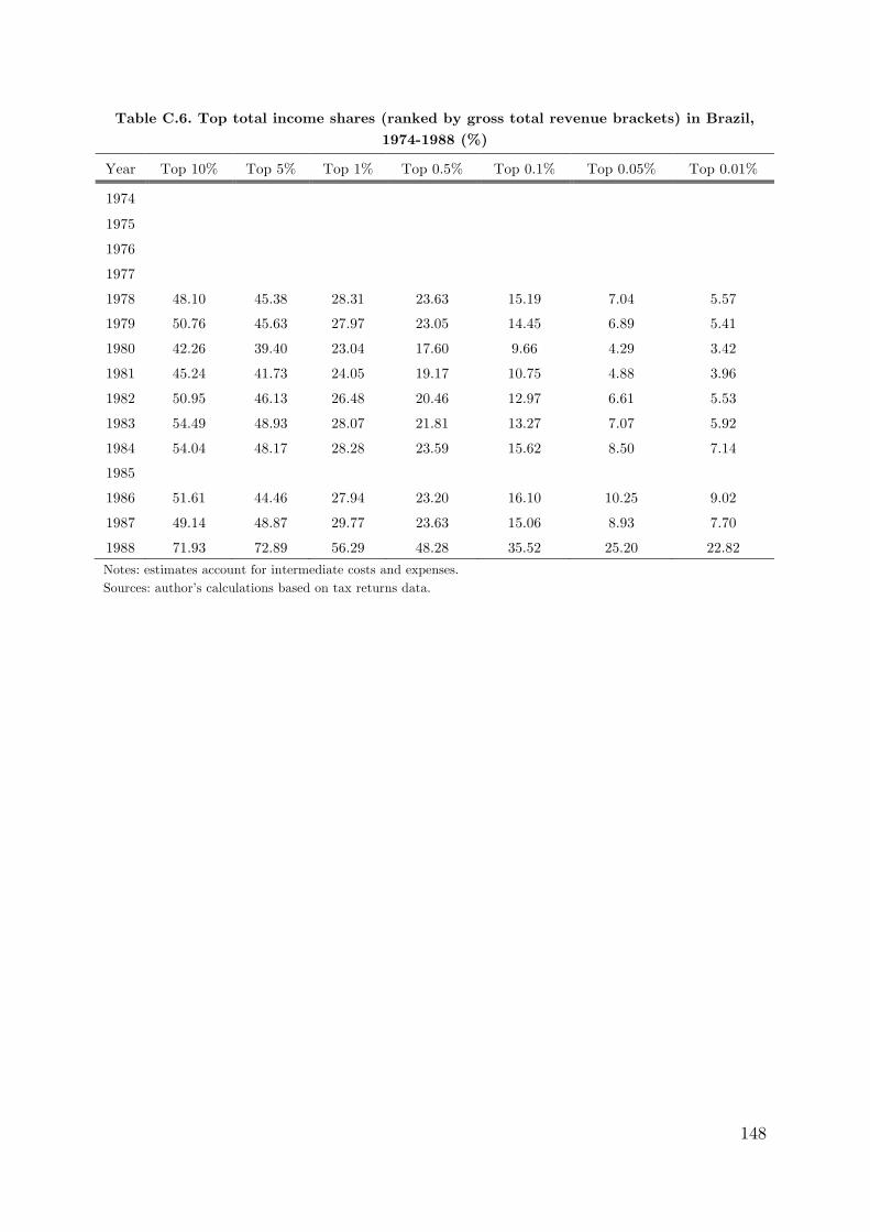
by brackets of gross taxable revenue could be calculated. Moreover, from 1978 to
1988 the publications contain tabulations that rank gross total revenue by brackets of
non-taxable revenue. This is useful information as the ranking variable of non-taxable
revenue turns out to more accurately capture the total income of individuals at the
very top of the distribution, given that non-taxable revenues appear to be
disproportionally concentrated among top groups, as compared to the total income
25 It is thus assumed that these proportions were maintained for the years before 1945. See Appendix C.2.2.
36
reported by brackets of gross taxable revenue. This is the effect of the growing scope
of non-taxable revenue from capital sources over time. As a result of this discrepancy
in the tax laws and statistics, I proceeded to use the non-taxable-bracketed
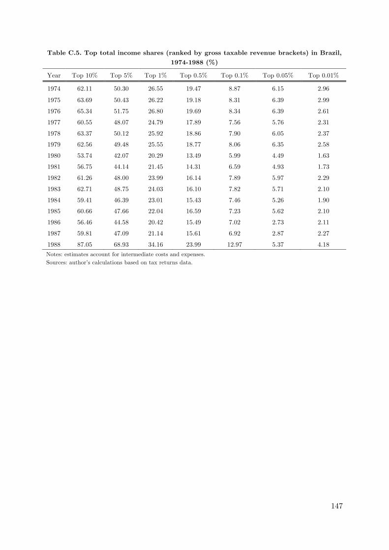
tabulations to estimate the shares of the top 1 per cent and above for the years 1978
to 1988, while resorting to the taxable-bracketed tabulations to estimate the shares of
the top 10 per cent and top 5 per cent of income earners between 1974 and 1988.26
The latter tabulations were used to approximate the shares of the top 1 per cent and
above for the years before there is data available on total incomes ranked by non-
taxable revenue brackets (i.e. before 1978). This is justified by the proximity between
the top 1 per cent total income series, ranked by gross taxable revenue and by non-
taxable revenue for the closest overlapping years until the early 1980’s, when both
series diverge.27 Given that most of the revenue of the top groups is non-taxable (as
evidenced by the tabulations) and in order to preserve continuity in the estimates,
the final series uses the tabulations ranked by non-taxable revenue to estimate the
shares of the top 1% and above from 1980 to 1987, while the ones ranked by gross
taxable revenue are used to estimate these shares from 1974 to 1979.
3.2 The definition of income used The income tax statistics for Brazil present a further challenge in appropriately
defining the pre-tax incomes of individuals from information reported to tax
authorities. As documented above, there are differences in the time series regarding
the reported income concept that can be observed. At this stage it is necessary to
emphasize that the ‘ideal’ definition of ‘gross income’ should deduct costs incurred to
26 In the final series, estimates for 1988 were left out due to them being notable outliers, as top shares increase by over 20 percentage points. This could be due to the hyperinflation that was taking hold of the period greatly benefiting top groups in relative terms or to typographical errors made by tax filers in their returns. For instance, there are only 31 taxpayers in the highest non-taxable income bracket in 1988, compared to almost 80,000 in 1987, yet their total non-taxable income amounts to 4 per cent of GDP. 27 See Figure in Appendix C.2.3.
37
obtain it. Unfortunately, the statistics only report this concept (after scheduler
deductions for expenses incurred) from 1969 to 1988. Moreover, the publications
provide little information about such expenses, simply noting the total value of
scheduler deductions that each income source has deducted per bracket. It is likely
that many costs and expenses are exaggerated by tax filers in order to reduce their
tax liability more than what a true calculation of real costs would allow, as in other
countries in the region (see Londoño Vélez, 2012, for the Colombia case).
Consequently, the estimates based on this gross taxable income (renda bruta)
are judged to underestimate top income shares. Conversely, estimates calculated on
the basis of the gross taxable revenue concept, before subtracting any costs incurred
to generate it (rendimento bruto), is deemed to overestimate top shares. Therefore,
the preferred series would lie somewhere in between.28 Without access to further
information, an average of the two series produced from the two gross taxable
concepts between 1969 and 1988 was calculated to approximate this preferred series.
In any case, taking gross taxable revenue without consideration of any deductions for
expenses would increase our estimates of the top 10 per cent income share by about 3
percentage points and the top 1 per cent by about 1 percentage point, on average.29
The difference between the gross taxable revenue series before deductions and this
preferred average series is assumed to also hold for years when there is only data for
gross taxable revenue (1998, 2002 and 2006-2013), and for gross total revenue for the
years 1974-1987 and 2006-2013, such that a preferred average series could also be
estimated for these series. The same procedure was followed in estimating the pre-
1969 period, after the extrapolation from net taxable income concept to the two gross
taxable income concepts was made.
28 This is assuming that there is no tax evasion, which is in practice untenable. To account for tax evasion, it might make more sense to use the series of gross revenue. See Appendix C.2.2 for results based all the series calculated from different income concepts. 29 See Figure C.5 in Appendix C.
38
To clarify, this preferred definition of income includes all income categories
reported in the personal tax returns (wages and salaries, self-employment, interests,
rents, business profits and dividends, agricultural income and other income), in
addition to non-taxable incomes, and it is before personal income taxes and employee
payroll taxes but after employers’ payroll taxes and corporate income taxes.
Unfortunately, the compositions of income made by income source, occupation gender
and decade of birth could only be made on the basis of gross taxable revenue, before
deductions for expenses, given that the definition of income after deductions was
unavailable for the relevant years in the publications. The reader assessing these
results must bear this in mind, although the overall compositions are unlikely to be
affected to a great extent.30
In summary, the main empirical contribution of this paper is to have
assembled a novel historical dataset on the distribution of income in Brazil,
characterized by its long time horizon and its scope in accounting for taxable incomes
as well as non-taxable incomes. Table 1 summarizes the main features of this
database, following the concepts and the extrapolation techniques mentioned above.
It can be noted that the top 5 per cent and 10 per cent are not estimated for the
years 1933 to 1967. This is due to the limited coverage of the income tax, which
collected returns for less than 2 per cent of the taxable tax units (see Figure 9 above)
– a direct result of having an exempted income tax threshold higher than the average
income per worker for the entire period (see Figure 8 above).
30 The relative shares would probably more affected for the income categories and nature of occupation than for the genders or decades of birth, given that some categories of workers may have more important deductible expenses than others. However, a more serious concern is the absence of non-taxable income from the compositions, which would affect the relative weight of the income categories and nature of occupation to a greater extent.
39
Table 1. Database on income distribution at the top in Brazil, 1933-2013
Panel A: observed series
Geographical level
Income years Income brackets Income reported Income groups covered
Federal District 1933 - 1950 Net taxable income Net taxable income Top 1 - 0.01% States 1943, 1945 - 1950, 1966 Net taxable income Net taxable income Top 1 - 0.01% Brazil 1945 - 1960, 1965, 1967 Net taxable income Net taxable income Top 1 - 0.01%
1968 Net taxable income Net taxable income Top 10 - 0.01%
Gross taxable revenue Gross taxable revenue Top 10 - 0.01%
1974 - 1987 Gross taxable revenue Gross total revenue Top 10 - 5%
1974 - 1979 Gross taxable revenue Gross total revenue Top 1 - 0.01%
1980 - 1987 Nontaxable revenue Gross total revenue Top 1 - 0.01%
2006 - 2013 Gross total revenue Gross total revenue Top 10 - 0.01% Panel B: extrapolated series
Geographical level
Income years Income shares Income groups
Brazil 1933 - 1960, 1965 - 1967 Gross taxable income Top 1 - 0.01%
1968 Gross taxable income Top 10 - 0.01%
Notes: Federal District is the city of Rio de Janeiro; state level data is for São Paulo, Minas Gerais, Rio Grande do Sul for 1943; Rio de Janeiro, São Paulo, Minas Gerais, Rio Grande do Sul, Goiás, Pará and Maranhão for 1946-1951 and Guanbara and São Paulo for 1966. The series for 1937, 1939-1941 go as far as the top 0.05%; 1942-1944 go as far as the top 0.1%; 1954 covers the top 0.5%-0.01%; 1985-1987 go as far as the top 0.1%, while 1988 only goes as far as the top 0.5%. The extrapolated series (Panel B) are adjusted for deductions towards expenses incurred to generate the income. Sources: database constructed by the author using tax returns.
3.3 Estimation method Since the income tax data are in the form of grouped tabulations, and since the
income intervals do not generally coincide with the percentiles of the population with
which we are concerned (such as the top 1 per cent, the top 0.1 per cent, etc.), we
resort to using Pareto interpolation techniques to calculate the desired shares of total
income, as well as estimating the threshold and average income levels for each fractile
we are interested in, as is usual in the top income literature since Kuznets (1953).31
31 This assumes that the top tail of the income distribution is well fitted by a Pareto distribution. In a Pareto distribution, the probability that income x is greater than threshold y is Pr(x > y) = 1 – F(y)
40
This paper also analyses the shape of the distribution among the tax paying elite, by
calculating the inverse Pareto-Lorenz coefficient β by income range, following the
approach presented in Atkinson & Piketty (2007, 2010).
This estimation method relies on the underlying data, described above, which
tabulates income taxpayers by ranges of income, but also on two further ingredients:
the construction of an external control for the potential number of total taxpayers
(i.e. tax units) based on demographic data; and the construction of an external
control for total income derived from National accounts data. The purpose of the
first control total is to be able to express the taxpayers in the tabulations as a
proportion of the total, so that the top 1 per cent refer to the top 1 per cent of
potential taxpayers, rather than the top 1 per cent of actual taxpayers. This
derivation is described in Section 3.4. The purpose of the second control total,
described in detail in Section 3.5, is to express the reported income of taxpayers as a
proportion of total household sector income. Therefore, this paper follows the
standard methodology used in the top incomes literature, which combines tax data
with external sources for the reference population and total income (see Atkinson &
Piketty, 2007, 2010).
3.4 Control total for population In order to relate the number of taxpayers to an external control total, there is a
need to know who is required by law to file a tax return. Unfortunately, the Brazilian
legislation is unclear as to the precise nature of the income tax unit. For example,
legislation was passed in 1943 that required the joint declaration of income by
= (c/y)α, where 1 – F(y) is the proportion of the population whose income is greater than y, c is a constant and α is the Pareto-Lorenz coefficient. The Pareto-Lorenz coefficient α can be calculated by regressing the logarithm of the reverse cumulative distribution, 1 – F(y), on the logarithm of the income level y. The parameters of interest are estimated using a characteristic property of power laws, which is that the ratio of average incomes above y to y is constant and independent of y (see Piketty, 2001).
41
married couples (Decree 5.844 of 23/9/1943, Article 67). However, evidence from the
tabulations between 1968 and 1988 suggest that married women could file a separate
tax return, the proportions varying from 3% of total taxpayers in 1968 to 12% in the
late 1980’s. So it remains unclear as to when the obliged joint declaration was
withdrawn.
I thus approximate the number of tax units (i.e. the number of individuals had
everyone been required to file for tax) by the working population, defined as all
residents aged 15 years and above, minus the number of married women aged 15
years and above for the period 1933-1967.32 From 1968 to 1988 the number of
married women filing a separate tax return is added to number of tax units. The
1998 tabulation decomposes the tax returns by sex, rather than by civil status, so
only the proportion of total tax returns filed by women is presented (the figure being
37 per cent). To arrive at the population denominator for the more recent years, it
assumed that the 1988 ratio between married women filing a separate tax return and
total women filing a separate tax return (around 67 per cent) is preserved for the
years 1998 and 2002 and for the period 2006-2013, such that the proportion of total
tax returns filed by married women is approximated to be 25 per cent for these years.
Thus, a quarter of the tax returns are added to the number of tax units over these
years.
All the population estimates are sourced from tabulations of population count
by age group for all decennial censuses since 1920 made by the IBGE. The annual
long run series for the population was estimated on the basis of interpolating the
observed growth rate between decades for each of the population units of interest.
32 The age cut-off in the international literature on top incomes generally varies between 15 and 20 years. In a developing country like Brazil there is room to believe that a non-negligible proportion of the population have historically entered in the labour market before 20 years of age. It is also reassuring that the population aged 15 and above is commonly used by the IBGE in its official household survey (the PNAD), while an age cut-off of 10 is usually used in the decennial Census, to estimate average incomes and other various labour market characteristics of the working population.
42
3.5 Control total for income The second step in the methodology is to define the income denominator. So as to be
able to calculate income shares for top groups and study income concentration, we
must relate the income amounts recorded in the tax statistics (i.e. the numerator of
the top share) to a comparable control total for the income earning population (i.e.
the denominator of the top share). This control total is essentially an estimate of
total personal income (or total income of the household sector as defined in National
accounts). And it would be the total personal income reported on tax returns if all
tax units had been required to file a tax return.
Since only a fraction of individuals filed a tax return in Brazil, the income
denominator cannot be estimated using the income tax data, but rather needs to be
estimated from National accounts. Following a similar procedure to the estimates
made for Colombia (Londoño Vélez, 2012), I approximate the income denominator as
the sum of households’ primary incomes and social benefits other than in-kind social
transfers, minus: (1) employers’ actual social contributions, (2) employees’ and self-
employed actual social contributions, (3) imputed social contributions, (4) attributed
property income of insurance policyholders, (5) imputed rents for owner occupied
housing, and (6) fixed capital consumption of households (assumed to be 5% of gross
fixed capital formation, as in Colombia). The only years for which detailed enough
data exists for this estimation are 2000 to 2011.
This procedure yields an average reference gross income of 60 per cent of GDP
at current prices between 2000 and 2011, which is broadly comparable to the average
reference figure for Colombia between 1993 and 2010 of 65 per cent of GDP, and
similar to the control totals for income used in the case of Argentina (Alvaredo,
2010) and Spain (Alvaredo and Saez, 2009). Due to the unavailability of detailed
National accounts data for the period prior to the 2000’s, the control total for income
was set at 60 per cent of GDP for the entire period of study. Caution here is needed
since, as Atkinson (2007) points out, applying a constant fraction for the control
43
total, computed on recent data, may not be an appropriate approximation of the
income denominator in earlier years, given the increasing importance of items such as
social contributions, pension funds and public transfers.33
4. Top income shares in Brazil, 1933-2013
Based on the methodology outlined above, the shares of personal income accruing to
top income groups are presented in the following section. Before documenting the
long-run dynamics of these shares, a preview of the orders of magnitudes will be
offered to place the findings into perspective. The section will also investigate the
composition of taxable incomes (into the categories mentioned previously), uncover
the extent to which top incomes are actually taxed, and finally, present Brazil’s
income concentration in an international comparative outlook.
4.1 Preview of magnitudes To give a sense of the orders of magnitudes of top incomes in Brazil, Table 2 presents
the thresholds and the average taxable incomes of different percentiles within the top
10 per cent of income recipients in 2013, while Table 3 presents the same information
for total incomes (combining statistics on taxable incomes, non-taxable incomes and
incomes taxed exclusively at source).34 In 2013, there were around 125 million tax
units in Brazil, with an average income of around R$ 24,500 (around US$ 14,500 in
PPP terms). From Table 2 it can be seen that in order to belong to the top 10 per
cent (P90) of taxable income recipients in 2013, a resident in Brazil needs to have a
yearly income of at least R$ 34,902 (around US$ 20,600 PPP). To belong to the top
33 The computation and sources regarding the control totals is explained in more detail in the Appendix B.1 and B.2. 34 Readers should note that the income reported is gross revenue, given that there is no information in the statistics regarding intermediate costs in order to calculate average income levels and thresholds of fractiles after deducting these expenses.
44
1 per cent (P99), one needs to make at least R$ 157,127 (around US$ 92,300 PPP)
per year. It can also be seen that the average yearly income of the top 0.01 per cent
(P99.99) was around R$ 3.7 million (about US$ 2.2 million).
Table 2. Thresholds and average taxable incomes in top groups within the top decile, Brazil 2013
Thresholds
Income level
(2014 R$)
Income level (US$, 2014
market exchange
rate)
Income level
(US$, 2014 PPP
conversion factor)
Income groups
Number of tax units
Average income
(2014 R$)
Average income (US$, 2014
market exchange
rate)
Average income
(US$, 2014 PPP
conversion factor)
(1) (2) (3) (4) (5) (6) (7) (8) (9)
Full Population 125,057,072 24,569 10,434 14,538
P90 34,902 14,822 20,652 Top 10-5% 6,252,854 45,942 19,511 27,185
P95 57,909 24,593 34,265 Top 5-1% 5,002,283 90,179 38,298 53,361
P99 156,127 66,304 92,383 Top 1-0.5% 625,285 197,903 84,046 117,102
P99.5 213,224 90,552 126,168 Top 0.5-0.1% 500,228 274,435 116,548 162,388
P99.9 402,287 170,844 238,040 Top 0.1-0.05% 62,529 544,446 231,217 322,157
P.99.95 1,041,113 442,143 616,043 Top 0.05-0.01% 50,023 1,224,034 519,826 724,280
P99.99 1,498,783 636,507 886,854 Top 0.01-100% 12,506 3,774,335 1,602,894 2,233,334 Note: Income assessed is gross taxable income, ranked by brackets of gross taxable income. Intermediate costs and expenses are not factored in due to a lack of information, thus the incomes reported equate to gross revenues. Amounts in US$ are computed using the average 2014 market exchange rate (US$ 1 = 2.35 R$) from the Banco Central do Brasil and the average 2014 PPP conversion factor (US$ 1 = 1.69 R$) from the World Bank.
If we account for total income (Table 3) we can observe that in order to
belong to the top 10 per cent, one now needs to make a little bit more – around R$
44,800 (around US$ 26,500 PPP). A larger threshold is observed if one wants to
belong to the top 1 per cent – one now needs a yearly income of at R$ 247,653 (US$
146,540 PPP). However, a notably larger change occurs at the very top, where, for
example, the average income of the top 0.01 per cent increases about seven-fold (to
around R$ 23.7 million, or approximately US$ 14 million PPP) if we account for
total income, rather than just taxable income. To get a better picture of the
difference each income concept makes to the thresholds, Figure 12 presents the
difference for each of the percentiles at the top. A clear trend emerges whereby the
higher up the distribution we go, the greater is the difference between the amounts of
45
total income, and those that are just taxable. This is evidence that non-taxable
income and incomes taxed exclusively at source are highly concentrated among the
very rich in Brazil.
Table 3. Thresholds and average total incomes in top groups within the top decile, Brazil 2013
Thresholds
Income level (2014 R$)
Income level (US$, 2014
market exchange
rate)
Income level
(US$, 2014 PPP
conversion factor)
Income groups
Number of tax units
Average income
(2014 R$)
Average income
(US$, 2014 market
exchange rate)
Average income
(US$, 2014 PPP
conversion factor)
(1) (2) (3) (4) (5) (6) (7) (8) (9)
Full Population 125,057,072 24,569 10,434 14,538
P90 44,885 19,062 26,559 Top 10-5% 6,252,854 59,024 25,066 34,925
P95 80,699 34,271 47,751 Top 5-1% 5,002,283 135,465 57,529 80,157
P99 247,653 105,174 146,540 Top 1-0.5% 625,285 304,466 129,302 180,158
P99.5 376,306 159,811 222,666 Top 0.5-0.1% 500,228 544,291 231,151 322,066
P99.9 963,378 409,130 570,046 Top 0.1-0.05% 62,529 1,725,490 732,785 1,021,000
P.99.95 4,591,946 1,950,119 2,717,128 Top 0.05-0.01% 50,023 5,724,228 2,430,980 3,387,117
P99.99 7,397,119 3,141,427 4,376,993 Top 0.01-100% 12,506 23,697,908 10,064,088 14,022,431 Note: Income assessed is gross total (taxable, non-taxable and taxed exclusively at source) income, ranked by brackets of gross total income. Intermediate costs and expenses are not factored in due to a lack of information, thus the incomes reported equate to gross revenues. Amounts in US$ are computed using the average 2014 market exchange rate (US$ 1 = 2.35 R$) from the Banco Central do Brasil and the average 2014 PPP conversion factor (US$ 1 = 1.69 R$) from the World Bank.
Figure 13 places Brazil’s top total incomes in a comparative perspective with
those of the U.S. A similar trend again emerges, whereby the difference between the
income levels in the two countries is generally lower the higher up in the distribution
we make the comparison. This illustrates that the elites in Brazil are pretty much as
rich as the elites in the U.S. A further point that can be noticed is that there appears
to be greater polarisation of incomes within the top 10 per cent in Brazil than in the
U.S. (comparing P90 and P99.99 in each country). This suggests that market income
in Brazil is more unequally distributed at the top than in the U.S.
46
Figure 12. Incomes at different percentiles in Brazil in 2013 (2014 Reais)
Notes: intermediate costs and expenses are not factored in due to a lack of information, thus the incomes reported equate to gross revenues. Sources: Author’s calculation for Brazil based on tax returns data.
Figure 13. Incomes at different percentiles in Brazil and US in 2013 (2014 PPP US$)
Notes: intermediate costs and expenses are not factored in due to a lack of information, thus the incomes reported equate to gross revenues. Estimates for Brazil include capital gains. Sources: Author’s calculation for Brazil based on tax returns data. WTID for U.S.
47
4.2 Long run dynamics of top income shares Section 4.1 revealed notable differences between top taxable income and top total
income, to a point where taxable income appear to be a severely underestimated
representation of the true income of the very rich, at least for 2013. The following
section shall present the shares of household gross income accruing to top groups over
the long run in Brazil, depicting the different dynamics characterising the shares
based only on the gross taxable portion of income and those based on gross total
income over the period.
Figure 14 displays the income share of the top 1 per cent in Brazil from 1933
to 2013 in two series, one for gross taxable income and one for gross total income.
The first point that can be noticed is the considerable difference between the levels of
the two series for the period after 1974, when data for the gross total income series is
available. Income inequality based on gross total income appears much larger than
what estimates based on gross taxable income would suggest. Between 1974 and 1980
the share of total income accruing to the top percentile was about 12 percentage
points higher, on average, than that of taxable income – in 1974 the top 1 per cent
total income share was 27 per cent (27 times the average income of the population),
while the taxable income share was around 14 per cent. Over the 1980’s this
difference increased to around 18 percentage points, with the total income share
reaching 30 per cent, while the taxable income share was of about 11-12 per cent. In
2013, the top percentile total income share registered a level of 27 per cent, while
accounting for only taxable income reduces this share to 11 per cent. The magnitude
in this difference alone is enough to suggest that a large chunk of the income of the
rich in Brazil is either taxed exclusively at source (at more favourable rates) or
exempt completely from the personal income tax.
In terms of trends, the top 1 per cent taxable income share followed a U-
shaped pattern between 1933 and 1972. The top 1 per cent share was halved from
around 20 per cent in 1942 to 10 per cent in 1959. This was at the same time that
48
the top marginal tax rate more than doubled, from 20 per cent in 1946 to 50 per cent
in 1947 (see Figure 10 above). Income concentration then increased as the political
crisis of the early 1960’s gave way to the military dictatorship of 1964, with the
taxable income of the top 1 per cent growing faster than that of the rest of the
population. It plateaued during the early 1970’s at a level of around 17 per cent.
Since then, the taxable income share of the top percentile has followed an L-shaped
pattern: experiencing a notable decline during the heyday of import-substitution
industrialization and rapid growth, and a quasi-stable evolution since the mid
1980’s.35 The 1970’s decline in inequality can also be observed from the total income
share of the top 1 per cent. However, from the 1980’s both series diverge, due
exclusively to the rise in inequality reported by the total income share. The widening
gap could be partly explained by the fiscal incentives granted to capital incomes
(which could benefit from lower rates if taxed exclusively at source) on the on hand,
and the relatively high and increasing fiscal pressure on top taxable incomes on the
on the other (see Figure 10 above). Since the late 1980’s, there appears to have been
no major alterations to the income share of the top percentile in general, despite the
gaps in the series.36 What can be clearly observed is that from at least 2006, income
concentration as measured by total income has been increasing, giving the Brazilian
‘success story’ something of a reality check. Even if measured by taxable income,
inequality experiences no significant decline, but rather a constant evolution.
A similar picture can be observed for higher points in the distribution. Figure
15 presents the evolution of the top 0.1 per cent share, while Figure 16 depicts the
dynamics for the top 0.01 per cent share, according to taxable income and total
income. It can be seen that the higher up in the distribution one examines, the lower
the volatility in the taxable income shares (the U-shaped pattern turns more into an
35 Readers should note that between the late 1980’s and 2006, there are too few data points to be able to properly judge the dynamics of top shares. 36 It looks to be the case that the total income share of the top percentile experienced a U-shaped pattern during this period.
49
L-shaped pattern for the entire period, especially for the top 0.01 per cent), and the
greater the volatility in the total income shares. This possibly reflects the fact that a
great proportion of the income of the top 0.1 and 0.01 per cent is made up of highly
cyclical capital incomes, especially capital gains, which are more accurately captured
in the total income series. As mentioned before, at present capital gains are taxed
exclusively at source while dividends and profits (reflecting ownership rights over the
means of production in society) are exempt from the income tax. At the same time,
the total income share of the top 0.01 per cent has been around 5 per cent (Figure
16). This means that the average income of this group (around 12,500 individuals) is
approximately 500 times large than the average income of the entire population.
Since 2006, this group has continued to strengthen its position, while its taxable
income share has remained quite stable. As was the case with the total income share
of the top 1 per cent, the same shares of the top 0.1 and 0.01 per cent experienced
strong gains during the chaotic years of stagnating average growth and hyperinflation
over the 1980’s. Thus, the rising shares over these years could simply reflect the
weakened relative position of lower income groups (those within the bottom 99 per
cent) with respect to higher income groups, due to the latter being able to better
protect themselves against inflation.
Figure 17 presents the estimates for the top 10 per cent, being concerned with
a shorter overall time-period for gross taxable income. The taxable income pattern is
the same L-shaped pattern as for higher income groups, with a decline from a level of
around 50 per cent in 1970 to a level of around 35 per cent the late 1980’s, and
relative stability over recent years. As expected, from what was mentioned above, the
evolution of the total income share of the top 10 per cent appears less volatile than
its counterparts higher up the distribution, and less distinct from the taxable income
share. This latter observation is the result of the top 10 per cent total income share
concentrating less of the capital incomes exempt from the income tax or taxed
exclusively at source. Again, it seems likely that a U-shaped pattern was followed,
50
with current shares of almost 60 per cent being close to late-1970 levels after steadily
rising over the seven-year period between 2006 and 2013.
Figure 14. Top 1% income share in Brazil, 1933-2013
Sources: Table C.3 and C.4.
Figure 15. Top 0.1% income share in Brazil, 1933-2013
Sources: Table C.3 and C.4.
51
Figure 16. Top 0.01% income share in Brazil, 1933-2013
Sources: Table C.3 and C.4.
Figure 17. Top 10% income share in Brazil, 1968-2013
Sources: Table C.3 and C.4.
Given that the inequality based in gross total income presents a more
complete and accurate picture of what is happening at the top of the distribution in
Brazil, the following analysis of the between and within share dynamics will primarily
focus on the estimates accounting for total income. Figure 18 begins by decomposing
52
the total income share of the top decile into three separate groups: the top 10-5 per
cent, the top 5-1 per cent and the top 1 per cent. It can be seen that the top 1 per
cent captured the majority of the gains over the 1980’s, with its share by over 5
percentage points, at the same time as the share of the top 5-1 per cent falls and the
share of the top 10-5 per cent remains roughly constant. Since 2006, all groups
experience gains, which are nevertheless greatest for the top 1 per cent group.
Figures 19 and 20 decompose the top 1 per cent and top 0.1 per cent into
similar groups. The polarised dynamics observed from the decomposition of the top
decile are brought out even more drastically for the higher groups. During the 1980’s
and 2000’s it was the income share of the top 0.1 per cent that experienced the
largest growth out of the three groups within the top 1 per cent (Figure 19). Looking
within the top 0.1 per cent, it is again the ultra-rich, the top 0.01 per cent, that make
disproportionate gains over similar periods. However, as with the top 0.1 per cent,
they are accompanied by the greatest volatility.37
The estimates revealed above provide evidence of inequality within the top of
the distribution in Brazil. In order to investigate this within-inequality more directly,
we can examine the level and trend of the inverse Pareto-Lorenz coefficient β = α/(α-
1), where α is the standard Pareto coefficient. The inverse Pareto-Lorenz coefficient
depicts the mean income above y as a multiple of y. If the income distribution at the
top were precisely of Pareto form, this ratio would be independent of y. In practice
the values of β are not constant, but usually lie within a fairly narrow range (Cowell,
2009). A higher value of β for any given year equates to a fatter upper tail in the
distribution and thus a higher degree of income concentration.
37 The relatively lower share of the top 0.05 per cent explains why the share of the top 0.1-0.05 is higher and the share of the top 0.05-0.01 lower than the equivalent shares decomposing the top 0.1 per cent in Figure 19.
53
Figure 18. Top income shares between the top 10% and top 1% by gross total income in Brazil, 1974-2013
Sources: Table C.3 and C.4.
Figure 19. Top income shares between the top 1% and top 0.1% by gross total income in Brazil, 1974-2013, top 1-0.1%
Sources: Table C.3 and C.4.
54
Figure 20. Top income shares between the top 0.1% and top 0.01% by gross total income in Brazil, 1974-2013
Sources: Table C.3 and C.4.
Figures 21 and 22 portray the inverted Pareto-Lorenz coefficients for the
taxable and total income series, respectively. The following findings present
themselves. Firstly, β coefficients for taxable income have fallen from levels above 2
at the beginning of the period to roughly 1.75 today. This is consistent with the fall
in income concentration reported by taxable income shares over the long run.38
Second, the β coefficients for gross total income depict greater concentration than
those for gross taxable income (as could be deduced from Figure 12 above), and a
higher degree of concentration over time with higher levels registered today than in
the mid 1970’s. It can be seen that today the coefficients vary between a value of 2.5
and 3, (in the late 1980’s they fluctuated between a value of 3 and 4), which equates
to extreme levels of concentration, consistent with the picture given by the top
38 For example a β of 2 means that the average income above the threshold needed to belong to the top 1 per cent is twice as large as this threshold. A value of 1.75 means that the average income above the 1 per cent threshold is 1.75 times the threshold value, which equates to a fall in top income concentration.
55
income shares. Moreover, income seems to be more concentrated greatest in the top 1
per cent within the top 10 per cent and the top 0.1 per cent within the top 1 per
cent, rather than within the top 0.1 per cent, as could be concluded from Figures 18-
20. Third, in using β as a summary measure of the shape of the upper part of the
distribution, we must bear in mind that its value depend on the points chosen in the
distribution, as Figures 21 and 22 help to convey. Nevertheless the close proximity of
each of the coefficient types is reassuring that the top of the distribution in Brazil is
quite well approximated by the Pareto structural form.
Figure 21. Inverted Pareto-Lorenz β coefficients for gross taxable income in Brazil, 1933-2013
Sources: Table C.7.
56
Figure 22. Inverted Pareto-Lorenz β coefficients for gross total income in Brazil, 1974-2013
Sources: Table C.7.
4.3 The composition of top taxable revenues As mentioned in Section 3, the tabulated data between 1969 and 1988 could be
decomposed into different components, relating to the source of revenue, the nature
of the occupation, the gender and age profile of top taxable revenue individuals. An
important qualification is that the data concern taxable revenues only, thus excluding
incomes taxed exclusively at source and non-taxable incomes, as well as scheduler
deductions for expenses incurred to obtain the income.
4.3.1 Revenue source
Figure 23 decomposes the taxable revenue share of the top decile into its various
sources and presents their evolution from 1969 to 1988. It can be seen that the large
majority of the taxable revenue of this groups comprises of employee remuneration,
basically wages. Over the course of twenty years between 1969 and 1988 the
importance of wages in the taxable revenue of the top 10 per cent increased – from a
proportion of 66 per cent in to 88 per cent by 1988. The counterpart of this increase
57
was largely the fall in the importance of self-employment revenue (from 16 per cent
in 1969 to 5 per cent in 1988).
The taxable revenue of the top 1 per cent offers a very similar picture (Figure
24), with slightly low shares of taxable revenue coming from employee remuneration
and self-employment, and a slightly higher share coming from rents, profits and
dividends. The dynamics are again very similar with the share of employee
remuneration increasing at the expense of self-employment revenue over the twenty
years. In order to notice considerable differences in the composition of taxable
revenue one must go to the summit of the distribution and assess the revenues of the
top 0.01 per cent (Figure 25). In the late 1960’s there was a more divided
composition of taxable revenues, with interests, rents and profits/dividends combined
making up a greater share of the taxable revenue of the ultra rich than employee
remuneration. However, by the mid 1980’s employee remuneration came to to
dominate these latter categories, with the self-employment contribution of self-
employment changing little.
Figure 23. Composition of top 10% taxable revenue by source in Brazil, 1969-1988
Sources: Table C.8.
58
Figure 24. Composition of top 1% taxable revenue by source in Brazil, 1969-1988
Sources: Table C.8.
Figure 25. Composition of top 0.01% taxable revenue by source in Brazil, 1969-1984
Notes: Estimates go up to 1984 only, since the tax statistics are not detailed enough to calculate the income share of the top 0.01% for the years 1985-1988. Sources: Table C.8.
A clearer way to see the radical changes in the composition of top taxable
revenues is if we aggregate the components into the broader categories of labour and
59
capital revenue. Figure 26 presents this type of decomposition for different fractiles
within the top percentile in 1969. It can be seen that as one moves further up within
the top 1 per cent, the share of labour revenue in gross taxable revenue falls. As one
enters into the top 0.05 per cent, capital revenue becomes dominant in the
composition of taxable revenue, while in the taxable revenue of top 0.01 per cent
mixed revenue becomes as important as labour revenue. 1984 displays quite adifferent
scenario for the summit of the distribution (Figure 27). We no longer see alterations
in the ranking of broad revenue categories as we move up the distribution, as labour
revenue maintains its overwhelming dominance over the other categories. This radical
change could be due to progressive erosion of the tax base over the years, whereby an
increasing portion of capital revenues could be taxed exclusively at source or be
exempt from the revenue tax altogether. This would confirm that much of revenues
of the very rich in Brazil are not accurately captured by the above Figures, as is
becoming increasingly evident in this paper. The fact that top shares according to
total revenue increased after 1980, while those according to taxable revenue
continued their downward trend, lends weight to this explanation.
Figures 28 and 29 decompose top taxable revenues into broad categories of
occupation from the earliest available data year, 1979, to the last available year,
1988. The notable lesson we can extract from Figure 28 is that in 1979 the large
changes across the distribution come from business owners replacing private sector
employees as the most representative of the very rich and the large loss in
representation of public sector workers as one moves higher up in the distribution.
The share of rentiers also experiences a notable rise across higher revenue thresholds,
trebling between P99 and P99.99. Within 10 years, the picture is stantially distinct.
Private sector employees experience no loss in representation across top groups; in
fact, their relative weight in the upper thresholds is increasing in the thresholds,
while the shares of business owners and rentiers is now significantly lower, even as
one moves into the top 0.1 per cent. Public sector workers now dominate both of
60
these latter occupation types. These compositions may appear to justify the
explanation that it is the erosion of capital revenues from the tax base that explains
the radical change in revenues of top groups during the 1980’s. In any event, judging
from the experience of other countries, the compositions presented here for Brazil do
not seem to be accurately representative of the real sources of revenue of elite groups.
Figure 26. Composition of top taxable revenues by source in Brazil in 1969
Sources: Table C.9.
Figure 27. Composition of top taxable revenues by source in Brazil in 1984
Sources: Table C.9.
61
Figure 28. Composition of top taxable revenues by nature of occupation in Brazil in 1979
Sources: Table C.10.
Figure 29. Composition of top taxable revenues by nature of occupation in Brazil in 1988
Notes: The tax statistics do not allow us to go above the top 0.1 percent in 1988. Sources: Table C.10.
62
4.3.2 Gender
Figure 30 decomposes top taxable revenue groups by gender in 1978, while Figure 31
presents the same decomposition twenty years later, for the last data point available.
In 1978 almost 20 per cent of the top 10-5 per cent taxable revenue group comprised
of women, while around 80 per cent were men (Figure 30). The higher up in the
distribution the smaller the representative of women, as one might expect, with the
female share falling to single digits among the ultra rich. From the 0.1 per cent
taxable revenue threshold, the share of women falls to about 4 per cent. Fast-forward
to 1998 and we are presented with a similar trend across top taxable revenue groups
(Figure 31). But while the share of men in top taxable revenue groups rises in similar
fashion to twenty years back, the levels from which it does so are much lower.
Among the top 10-5 per cent, the share of women has rise to 37 per cent from its 19
per cent level in 1978. This share falls steadily until it reaches a level of 18 per cent
for the uppermost taxable revenue groups (top 0.1 per cent and beyond). Thus, on
the basis of taxable revenue alone, one can conclude that women made notable
revenue gains over the twenty-year period.
Figure 30. Composition of top taxable revenue groups by gender in Brazil in
1978
Sources: Table C.11.
63
Figure 31. Composition of top taxable revenue groups by gender in Brazil in 1998
Notes: The highest population group we can estimate with the 1998 tabulations is the top 0.1 percent. Sources: Table C.11.
4.3.3 Generation
The final decomposition presented, concerns the relative age of top taxable revenue
groups. Figures 32 and 33 present the composition of taxable revenue by year of birth
of top earners for 1970 and 1988, the earliest year and last year for which data can be
extracted. In 1970 (Figure 32), the top 10-1 per cent of the taxable revenue
distribution were dominated individuals born between 1931 and 1940 (meaning they
were between 30 and 39 years of age in 1970). As one moves into the top 1 per cent,
and especially into the top 0.1 per cent, it is the older generations that dominate the
representation, i.e. those born no later than 1930 (persons aged over 40). In
particular, 55 per cent of the top 0.01 per cent is comprised of persons aged over 50
(or born on up to 1920), which is somewhat expected given that Brazil may not have
yet had the sufficient time to develop the productive capacities of its younger
generations by late 1960’s.
64
By 1988 (Figure 33), the age profile of top taxable groups had changed quite
notably. Among the top 10-0.5 per cent in the taxable revenue distribution, it was
the younger generations that were most represented, those born from 1941-1950
(aged between 38 and 47), and especially those born since 1951 (aged under 38). This
latter age category accounted for 52 per cent and 45 per cent of the individuals in the
top 10-5 per cent and 5-1 per cent respectfully, while in 1970 (aged under 20) they
made up hardly 1 per cent of the individuals, as one would expect. However their
share falls dramatically to 15 per cent among individuals within the top 0.1 per cent
in 1988. Yet over the course of 18 years it can be said that there was inter-
generational mobility in Brazil, at least for the portion of revenue that was taxable.
This can be again observed if we move higher up in the distribution. In 1970, the top
0.1 per cent and beyond was largely composed of individuals born no later than 1930
(aged 40 and above at the time). By 1988, these generations (born up to 1920 and
between 1921 and 1930) provided the lowest amount of individuals to the top 0.1 and
above (see Figure 33). At the very top of the distribution in 1988, we observe that
the greatest representation comes from individuals born between 1941 and 1950 (aged
between 38 and 47). Moreover, between 60 and 65 per cent of the ultra rich in this
distribution comprise of individuals aged between 38 and 57, which coincides with an
image of working professionals. This image seems consistent with earlier
decompositions, which presented salaried workers in the private and public sectors as
being the ‘typical’ rich individuals in the taxable revenue distribution.39 This profile
also seems to be consistent with those of the richest individuals usually captured in
household surveys.
39 It should be emphasized again, that the data do not allow us to evaluate the inter-generational mobility in the total income distribution, which may well present a different scenario.
65
Figure 32. Composition of top taxable income groups by year of birth in Brazil in 1970
Notes: being born up to 1920 corresponds to an age of 50+ in 1970; 1921-30 corresponds to being 40-49; 1931-1940 to 30-39; 1941-1950 to 20-29; and being born from 1951 corresponds to being under 20 years of age. Sources: Table C.12.
Figure 33. Composition of top taxable income groups by year of birth in Brazil in 1988
Note: being born up to 1920 corresponds to an age of 68+ in 1988; 1921-30 corresponds to being 58-67; 1931-1940 to 48-57; 1941-1950 to 38-47; and being born from 1951 corresponds to being under 38 years of age. Sources: Table C.12.
66
4.4 International comparisons The income disparities in Brazil revealed in the previous section can be emphasized
further if they are placed in an international comparative perspective. Figure 34
begins the cross-country comparison with a look at income concentration in the
region of Latin America. At the time of writing, Brazil is the fourth country in this
region where top income shares have been estimated using tax data, after Argentina,
Colombia and Uruguay. In a region known for top ranking inequality indices, Brazil
stands out for its degree of income concentration as can be observed from the relative
shares of the top percentiles in Figure 34. The top percentile share of total income
has been higher in Brazil than in any over its neighbours over the 2000’s, the years
for which we can make valid comparisons. It can be seen that the top 1 per cent in
Argentina and Uruguay rank closer to the top 1 per cent taxable income series in
Brazil. Colombia is closer to the overall income concentration registered in Brazil,
since 2006, but while the share in Colombia appears to stay roughly constant (also
the case in Uruguay between 2009 and 2012), in Brazil, the share undertakes a sharp
upward trend. Brazil’s current inequality appears to be even higher than that
observed in Argentina during its peak in the 1940’s. Although, comparative data is
more scarce for the years prior to the 2000’s, it is likely that Brazil’s historical levels
of total income concentration rank among the highest ever observed in the region,
especially if the historical trend in the gross taxable series and its difference with the
gross total income series are anything to go by.40
Figure 35 compares inequality in Brazil with that in developing countries
outside of Latin America (Asian countries and South Africa). The picture confirms
40 It can be noted that between the early 1930’s and the late 1950’s, the dynamics of the top percentile share in Argentina mirrored and the top percentile taxable income share in Brazil were hugely similar, with the shares in Argentina slightly higher. It should be bore in mind that the estimates for Latin American countries other than Brazil may be underestimated given that they don’t account for capital gains or some parts of capital income that is not taxed. In general, comparatbility with most countries must be taken with a pinch of salt given the large absence of capital gains from the estimates. Estimates including capital gains are stated wherever possible in the comparison graphs below.
67
Brazil as being an extremely unequal country even among underdeveloped countries.
South Africa has often been compared to Brazil for have similar levels of inequality,
but tax data suggest that there is quite a margin between the two, while comparison
with Asian countries confirms the inherited belief that Latin American inequality, is
on another level, particularly in Brazil. The U-shaped evolution depicted in South
African and Indian inequality does not appear to be followed in Brazil, even for
inequality based on gross taxable income, which depicts an inverted-U-shaped
pattern over the twenty or so years of the military dictatorship (1964-1985) when
inequality in all the developing countries was either stable or falling.
Figure 34. Top 1% income share in Brazil and Latin American countries, 1932-
2013
Sources: Table C.4 for Brazil and WTID for other countries
68
Figure 35. Top 1% income share in Brazil and developing countries outside Latin America, 1913-2013
Sources: Table C.4 for Brazil and WTID for other countries.
A similar picture presents itself for the top 0.01 per cent (Figure 39). The
principle difference is that over the recent few years, the share of the top 0.01 per
cent in the U.S. (accounting for capital gains) matched, if not slightly surpassed, that
in Brazil. But again if historical standards are to be set, the 1980’s in Brazil remain
an unprecedented period for the concentration of income at the very summit of the
distribution. The real extent of inequality in Brazil can also be seen from the
similarity between taxable income top shares in Brazil and total income shares in
other countries, such as Japan or Spain (outside of finance-induced boom phases) and
the U.S. prior to the 1980’s, given the significant portion of top incomes excluded for
the income tax in Brazil. This comparison can be made at all the fractiles in the
distribution, and the same conclusion is reached: Brazil is a highly unequal country
even when we mainly focus on labour income.
69
Figure 36. Top 1% income share in Brazil and selected developed countries, 1913-2014
Note: Other than Brazil’s total income series, capital gains are included in estimates for Canada (from 1972), Japan (from 1947), the US, Spain and Sweden. The UK and France are included for comparative purposes with Brazil’s gross taxable income series. Sources: Table C.4 and WTID.
Figure 37. Top 1% income share in Brazil and US, 1913-2014
Sources: Table C.4 and WTID.
70
Figure 38. Top 0.1% income share in Brazil and selected countries, 1913-2014
Note: Estimates for Japan and Spain include capital gains. Sources: Table C.4 and WTID.
Figure 39. Top 0.01% income share in Brazil and selected countries, 1913-2014
Note: Estimates for Japan and Spain include capital gains. Sources: Table C.4 and WTID.
Finally, we can compare the fatness of the upper tail of the distributions
across different countries, which describe how relatively unequal the top of the
71
distribution is. Figure 40 does this by placing the inverted Pareto-Lorenz coefficient
in Brazil in an international comparative perspective. The inequality at the top
revealed from Brazil’s gross taxable distribution was comparable to that in most
depicted countries for most of the last century. However, based on gross total income,
Brazil is near the top of the rank. During the 1980’s the upper tail in Brazil was
fatter than in any other distribution in the world. Inequality within top remains
highest in recent years, slightly above levels observed in the U.S. (as Figure 13
already hinted). Inequality within top groups is also of similar magnitude in
Argentina (although 2004 is the latest point available at the time of writing) and to a
lesser extent Colombia. Brazil is thus a world leader in income inequality, both in
terms of absolute differences between top groups and the rest, and relative differences
among individuals at the top.
Figure 40. Inverse Pareto-Lorenz β coefficients in Brazil and selected countries, 1913-2014
Sources: Table C.7 and WTID.
72
5. Discussion
5.1 Measurement issues When estimating top income shares, the presumption is often made that the share of
the rich has been accurately measured, more so than estimates from other data
sources. In the results presented above, I assumed (for comparative purposes) that
what was being measured was the true income share of the rich in Brazil. But there
are numerous reasons why the Brazilian estimates may not precisely reflect the
picture at the top. First, as was mentioned in Section 3, the estimates for Brazil are
constructed on the back of various assumptions regarding the external control for the
population (the appropriate age-cut off and the legal definition of the tax unit), the
external control for income (the constant proportion of GDP) and the income
concept captured by the estimates (the average between gross revenue before
deductions and gross income after deductions). These various methodological choices
were justified to the best possible extent, given the data available at the time of
writing. In any case, tweaking the assumptions leads to a change in top share levels
rather than underlying trends.41
A more prevalent concern is the degree of tax evasion, which in a developing
country like Brazil would seem justified. Changes in the amount of income
purposefully evading taxes can cloud the analysis of the dynamics of income
concentration. These changes can be triggered by changes in tax rates or legal
changes in the definition of deductions and allowances. For instance a rise in top
incomes may simply reflect reduced incentives for evading taxes when tax rates are
cut. This has been postulated about countries like the U.K. and the U.S., who both 41 For example, Medeiros et al. (2015), using the same underlying tax data, take the definition of the tax unit to be individuals aged 18 and over, and a definition of income to be prior to deductions for intermediate costs. In our judgment these are less preferable choices. The former choice corrects our results downwards, while the latter choice corrects them upwards. The net result is an almost indistinguishable series from the one calculated in this paper for the period 2006-2012, with differences below 1 percentage point (see Figure 48). However, we deem our estimates to be preferable given that our income concept is more accurate.
73
experienced sharp reductions in their top marginal tax rates since the 1980’s and a
strong rise in top income shares (see Figures 36 and 43). However, in Brazil the
relationship is not clear cut and sometimes contrary to expectations. Top shares of
gross total income doubled from 1980 to 1983, at a time when the top tax rate rose
by 5 percentage points from 55 per cent to 60 per cent, while they changed little
when the top tax rate fell from 60 per cent in 1985 to 45 per cent in 1988. Also
important legal changes to deductions and allowances took place during the tax
reforms of the early 1990’s, which abolished the scheduler system of taxation, along
with all its deductions. Since 1997 the top rate has remained unchanged at 27.5 per
cent and there has been no notable changes to the definition of deductions or
allowances, yet top shares have been on a strong upward trend since at least 2006.
There is thus very little evidence to suggest that the changes in the distribution of
income in Brazil were significantly affected by shifts in tax rates or legal changes to
deductions and allowances. Rather, they are more likely to reflect real economic
changes.
The dynamics of top shares can also be affected by improvements in tax
collection, in that such improvements may equate to stricter enforcement criteria and
technology allowing the tax office to better measure (and hence tax) the incomes of
the wealthy. In Brazil, there have been various stages of modernisation of the tax
collection agency since the introduction of the income tax, particularly during the
early 1940’s and in the late 1960’s. So for instance, the peak in taxable income
concentration observed in the early 1940’s in Brazil could have more to do with these
types of improvements than with real distributional changes in income. A similar
story could hold for the rise in inequality over the late 1960’s, upon the initiation of
the Federal Tax Office and the creation of a national identification system of taxable
74
persons.42 Unfortunately, we do not dispose of the necessary data to investigate the
likelihood of the inequality dynamics being due to better tax collection, such as
adequate data on the wage distribution.43 Therefore, the capacity to distinguish
between statistical mirages caused by improvements in tax collection and
enforcement from real distribution changes is a major limit of this study. In spite of
this limitation to interpret the trends, the main qualitative finding remains valid:
Brazil’s levels of income concentration are among the highest ever recorded.
A further issue to consider is the impact of Brazil’s shadow economy on
estimates of top shares derived from tax data, which largely miss income from
informal and underground activities. Accurate measures of the shadow economy are
difficult to come by, but the estimates on the relative size of this sector in Brazil
range from about 20 per cent of GDP to nearly 40 per cent of GDP for recent years
(Filho, 2012; Schneider et al, 2010). While the tax statistics capture much self-
employment income, it is likely that some portion of informal self-employment eludes
taxation. However, this is unlikely to be an important source of income for the rich in
Brazil, given the country’s large landed wealth and the important industrial and
corporate sectors. For the same reasons, wealth from illegal goods trade is not likely
to pervade the Brazilian economic elite, compared to other countries in the region
like Colombia. In any case, the national accounts-based estimate of the income
42 At the same time, a new income schedule was introduced for all incomes not attributable to the other existing schedules (Da Nóbrega, 2014) This may have uncovered income previously undeclared due to the fact that it did not fit any of the existing income categories. 43 Since wages are less subject to tax evasion than other sources of income (given the existence of certain wage related deductions, like the desconto padrão in Brazil) the dynamics of top wage shares can be compared to those of top income shares to uncover whether there is evidence of better tax collection. In such a scenario, one would expect wage incomes to have slower growth than other incomes (see Banerjee and Piketty, 2010 for an example of how this procedure was used in the case of India). As is evident from Section 4.3, the wage composition of income in Brazil can be uncovered for the taxable portion of income between 1969 and 1988. However, individuals are ranked by gross taxable income rather than by gross wages, which does not give a precise picture of the actual wage distribution.
75
control used in this paper takes into account flows of income sourced from the
shadow economy.
Perhaps the most important measurement issue concerns the relation of
inflation to the estimated top shares. High inflationary pressures plague Brazil’s
history, most notably the hyperinflation that took hold of the country from the
1980’s to the mid 1990’s. In fact prior to this, annual inflation rates consistently over
15 per cent were not uncommon. Figure 41 shows the evolution inflation (measured
indirectly using the GDP deflator) alongside the dynamics of the top percentile over
the long run in Brazil. Before the Second World War relatively high inequality in
Brazil seemed to coexist with low inflation. Yet from 1945 to the military coup of
1964 the decrease in reported inequality (of taxable income) was correlated with a
strong and persistent increase in inflation (the average annual rate over the period
was 24 per cent, with inflation peaking at 90 per cent by 1964). Given that the
majority of top taxable incomes are in the form of wages and self-employment income
(see Figures 23-25), it is likely that rising inflation had a lot to do with the falling
taxable income concentration.44 Overall, the inflation rate and the taxable income
share of the top 1 per cent appear to have a relatively strong inverse relationship.
Examining the gross total income series, its relation with inflation is less clear-
cut. On the one hand, the decline in total income concentration from 1974 to 1980
coexisted with high and rising prices (inflation more than doubles over the period
from about 35 per cent to 90 per cent). On the other hand, the dramatic rise in total
income inequality over the 1980’s came when inflation was progressing at its fastest
ever rate (the annual average was over 200 per cent). Although data is not available
44 The increase observed from the mid 1980’s could have been due to a growingly unequal indexation of prices and incomes to the rapidly rising inflation, which was institutionalized in Brazil from the late 1960’s until the mid 1990’s. Until 1979, nominal wages increased once every year, after which they increased twice a year until 1985. From 1985 to 1987 they were subject to revisions roughly every 3 months, and then every month until the mid 1990’s (Saad-Filho & Mollo, 2002) It is likely that the more frequent revisions were to the benefit of higher earning individuals, who as top executives and business owners have more control over their compensation packages.
76
to make the evaluation, it is likely that total income concentration remained
approximately at its late 1980’s level until the Plano Real in 1994. Moreover, since
2006 inflation has remained quite stable at a relatively low average of approximately
6 per cent per year, while total income inequality has risen by 16 per cent, close to
levels observed in the late 1980’s.
Figure 41. Top 1% income share and inflation in Brazil, 1933-2013
Sources: Table C.4 and Table B.3.
Thus, the role of inflation in explaining the dynamics of top shares (as
measured by gross total income) seems to be strongest during the 1980’s. A wide
literature has tried to evaluate the distributional consequences of inflation, commonly
known to be a regressive tax, as the capacity to protect the value of one’s portfolio is
generally increasing in income and wealth (Ferreira et al. 2007).45 In a survey of poor
households in 38 countries between 1970 and 2000, Easterley & Fischer (2001) show
45 Rich individuals have larger and more diversified portfolios than the average individual, and thus can more easily transfer their wealth into assets whose real income stream are more robust to inflation. Also wage indexation is usually to be more ‘perfect’ for richer individuals who control their own remuneration, such as top executives and business owners.
77
robust evidence that the share of bottom quintile of the distribution in national
income is lower and the real minimum wage also lower during periods of high
inflation. In the case of Brazil, Ferreira & Litchfield (2001) find that between 1981
and 1995 higher inflation was associated to a lower income share for the poor.
Coupled with the fact that between 1980 and 1990 the minimum wage lost 43 per
cent of its real value, the rising top total income shares during the 1980’s seem to be
a product of the worsening relative position of lower groups in the distribution, as
well as absolute gains in real income of top groups. Figure 42 illustrates this,
comparing the average income of the top 1 per cent with the average income per tax
unit and the average yearly minimum salary (average monthly minimum wage
multiplied by 12). Between 1980 and 1987, while the real minimum wage fell and the
average real income per tax unit stagnated, the top 1 per cent made real gains of 32
per cent. On the contrary, the 1970’s decline and the recent rise are more likely
explained by real economic and distributional changes, than by changes in inflation.
It is also interesting to note the magnitude difference between the average income of
the top 1 per cent and those of other population groups. In 2013, the average real
income of the top percentile was about 27 times the average real income per tax unit,
while about 77 times the average real yearly minimum salary.46 Such magnitudes
underline to a further extent the actual polarisation of income in Brazilian society.
46 According to the 2010 Census there were approximately 44.5 million individuals aged 10 and above earning the monthly minimum wage or less, which counts for about 27 per cent of the respective population (IBGE, 2010). In the same year, the top 1 per cent comprised of roughly 1.6 million of the same population.
78
Figure 42. Average real income of top 1%, average real income, and real minimum wage in Brazil, 1933-2013
Note: The average income per adult is the average income of all persons aged 15 and above minus the number of married women aged 15+ not filing a separate tax return. The first legislated minimum wage was introduced at the urban state-level in 1940. It was extended to rural workers in 1963, and a nationally unified minimum wage at the federal level was introduced in 1984. Since 2000, supplementary rates could be introduced by states on top of the national rate. 1 Brazilian Real ≈ 0.59 US Dollars PPP (2014 prices). Sources: Table B.3. and Table C.2.
5.2 Taxation of top incomes The large difference between top taxable income shares and top total income shares
uncovered in Section 4.2, especially for recent years, implies that a large part of the
incomes of the rich have been, and continue to be, untaxed. Our knowledge of the
profile of the rich in other similar countries also cast doubt over the
representativeness of the compositions of top taxable incomes shown in Section 4.3.47
Coupled with the extortionately high levels of pre-tax inequality for total income
revealed in Section 4.2, these findings put into question the role of taxation
concerning top incomes. Income taxes can have a pure redistributive effect by
discouraging the disbursement of very high gross incomes to individuals. But this
47 In countries like Argentina and Colombia, individuals primarily living off capital income typically characterize very top income groups. See Alvaredo (2010) and Londoño Veléz (2012).
79
depends on the legal definition of the tax base as well as the progressivity of the tax
rates, which is itself dependent on discretionary legislation on tax schedules and the
tax base. The current progressivity of top marginal income tax rates was questioned
in Section 2.3 due to the relatively few income tax brackets and a relatively low top
rate (see Figure 10). Despite Brazil having a top marginal tax rate comparable to
rich countries in the 1980’s, it currently lags behind OECD countries, including two
of its regional peers, Chile and Mexico (see Figure 43).
Figure 43. Top marginal income tax rates in Brazil in a comparative perspective, 1900-2013
Sources: Memória Receita Federal for Brazil, Piketty (2014) for U.S., U.K. and France and OECD for Chile and Mexico.
As emphasized, the findings conveyed thus far, point towards a very limited
definition of the tax base in Brazil, which can feed back into the effective
progressiveness of the overall tax system. Figure 44 illustrates this by plotting the
average income tax rate, on the portion of legally taxable income, and the effective
income tax rate, on total income, for top income groups in Brazil in 2013. A very
clear result emerges: the income tax schedule is regressive when the total income of
top groups is considered. It can be seen that the average tax rate is progressive across
80
top groups, with richer individuals paying a higher fraction of their taxable income to
the state (the average tax rate curve is positive sloping throughout the top of the
distribution). However, when total income is considered as the denominator,
progressivity falls beyond the top 0.5 per cent (the effective tax rate curve begins to
have a negative slope above the percentile P99-99.5), since richer individuals pay a
smaller fraction of their income. Moreover, it can be seen that the effective rate is
extremely weak, being about 3 per cent for the top 0.01 per cent; while at the same
time their average rate on their taxable income is in the range of 25 per cent.
Figure 44. Average and effective income tax rates for top groups in Brazil, 2013
Note: the average tax rate is calculated by dividing total net personal income tax liability (tax paid + tax due - tax refundable) by taxable income after legal deductions. The effective tax rate is calculated by dividing the same tax liability by total income (taxable income, non-taxable income and incomes taxed excl. at source), after deductions. Social contributions are excluded from the calculation due to the absence of data. Sources: Table D.1.
The extremely low tax burden for the ultra rich can explain why they account
for such a large share of household sector income, as well as the highly limited
redistributive capacity of the income tax in Brazil. Explaining the low effective tax
liability is the inferred hypothesis that this paper has come to reveal, namely the
large share of the income of the rich in Brazil that is not subject to the income tax.
81
Figure 45 helps to validate this hypothesis by depicting the extent of income subject
to the income tax in Brazil in 2013. The pattern is consistent with what has been
previously exposed – the taxable portion of income of individuals declines as one
moves up the distribution. It can be seen that this decline is quite drastic. 80 per
cent of the total income of the top 10-5 per cent of income recipients (P90-95)
comprises of taxable income, that is income subject to the income tax. This
proportion drops to 43 per cent for the top 0.5-0.01 per cent, before falling further to
reach an extremely low level of 13 per cent for the top 0.01 per cent in the
distribution. The counterpart to this decline is evidently the rise of income not
subject to the income tax across the distribution, namely non-taxable or exempt
income and income taxed exclusively at source. For the ultra rich, it can be observed
that the majority of their income is not subject to the tax (above 60 per cent for
individuals above the top 0.1 per cent in the distribution). This can be largely
explained by the fact that profits and dividends are exempt from the income tax. The
share of income taxed exclusively at source also rises with income, with the income of
the top 0.01 per cent concentrating three times more incomes taxed at source than
approximately the top 10-1 per cent. This can be explained by the fact that currently
in Brazil capital gains are taxed exclusively at source.
One may think these tax trends to be a recent phenomenon in Brazil,
especially since the tax reforms of the market liberalization period of the 1990’s.
However, on the basis of historical data available, this seems to be an erroneous
conclusion. In fact, well before the Washington Consensus, Brazil had an extremely
similar pattern of top incomes being subject the income tax as the one it has today.
Figure 46 presents the case for 1983, when Brazil was still under military
dictatorship. It be clearly seen that the share of taxable income in the total income of
individuals across top groups in 1983 was almost identical to what it is 30 years later.
Around 70 per cent of the income of the top 10-5 per cent was subject to the income
tax. This share falls sharply over the upper parts of the distribution, accounting for
82
roughly one-tenth of the income of individuals within the top 0.1 per cent.
Unfortunately, the data does not allow for a separation of non-taxable income from
income taxed exclusively at source, whose combined share of total income reaches 90
per cent for those within the top 0.1 per cent of the distribution.
Figure 45. Taxable income across top groups in Brazil, 2013
Sources: Table D.2.
Figure 46. Taxable income across top groups in Brazil, 1983
Sources: Table D.2.
83
5.3 Comparing tax data and household surveys All previous studies on the extent of income inequality and its relation to economic
growth in Brazil (with the exception of this paper and Medeiros et al. 2015) have
relied exclusively on household survey data, either to approximate the income share
of different fractiles (deciles, quintiles, etc.) or the level of overall inequality captured
in indices (Gini, Theil, etc.). Recent pursuits in the top incomes literature have
ventured into the comparison between tax data and household survey data, in order
to address the differences in their respective capacities to accurately approximate the
distribution of income. This development has become an upmost priority in many
regions, but none more so than in Latin America, where the use of surveys is
probably most widespread (see Alvaredo, 2011; Londoño Vélez, 2012 and Burdín et
al. 2014, for comparisons made in Argentina, Colombia and Uruguay respectively).
Alongside comparisons made in developed regions (Burkhauser et al., 2012 for the
U.S. for instance) the general consensus is that household surveys either completely
miss information on the top of the distribution or severely under-report it when
captured. The former may arise for a number of reasons, the most common being:
random exclusion due to random sampling, deliberate exclusion (ex-post) due to
minimize the bias in the estimates caused by extreme observations, and un-response
by the rich (given that there is nothing at risk by refusing to cooperate). Under
reporting even when the rich are captured in the surveys arise mainly because they
may feel more uncomfortable with disclosing their income and wealth on a
questionnaire (than on a tax form) or, even when they are willing to accurately
disclose their income streams, the nature of their portfolios may be such that the
total extent of their income is difficult to measure. Additional differences between
household surveys and tax data may arise in their units of observation (households or
individuals), in their definition of income (market income, gross income, net-after-tax
income, etc.) and their population and income coverage.
84
These differences make it crucial to understand the degree to which tax data
can say something about an aspect of income inequality that is not generally well
captured in surveys, namely the summit of the distribution. This is even more
important when changes in the inequality measured by surveys can be impacted by
changes in top income shares as measured by tax data (Atkinson, 2007). Therefore,
to fully evaluate income concentration in Brazil, the usefulness of survey data to
study top income shares and the degree to which tax data can complement household
surveys in approximating the overall distribution of income should be assessed. This
requires us to avail of survey micro-data so as to be able to extract an equivalent
distribution for the comparison with tax data.48 Unfortunately, the necessary survey
statistics to make such an assessment were not readily accessible to us at the time of
writing.49 Thus, the comparisons made in this Section are preliminary, and concern
time series comparisons between our estimates using tax data and existing series
using survey-related data.
Figure 47 presents different estimates for the income share of the top 10 per
cent, including our estimates based on tax returns for gross total income and gross
taxable income. It is apparent that the distribution of income and its dynamics in
Brazil varies considerably according to the nature of the data used for the
estimations, even for the top decile, whose income characteristics should be better
represented in surveys than higher income groups. 50 For recent years, income
concentration seemed to be declining since the early 2000’s according to the widely
cited household per capita income measure derived from Brazil’s principle household
survey, the Pesquisa Nacional por Amostra de Domicílios (PNAD), by the IBGE. On
the contrary, tax data show a mildly increasing trend for taxable income and a
48 Specifically, this means taking gross individual income from all sources, of all persons aged 15 and above. 49 This will be a pursuit of future research. 50 It should be borne in mind that the comparisons presented in Figures 47 and 48 do not relate to the same income concepts or population. See the notes to the two Figures.
85
strongly increasing trend for total income. The difference in magnitudes between
survey data estimates and tax data estimates (based on total income) is also stark
and increasing due to the diverging trends, implying that using household surveys
presents a highly distorted picture of the distribution.51 Estimates made by Medeiros
et al. (2015) from tax data on total income concentration begin at the top 5 per cent
(due to their tabulations being less detailed), but they can be combined with survey
data to approximate the an income share for the top 10 per cent. It can be seen that
the resulting series is very similar to our estimates, with the exception of the last few
years, where our series depicts a greater rise in inequality.
During the 1970’s and 1980’s, estimates from survey data continued to lie
between the two tax-based estimates, although survey-based estimates on gross
individual income appear to better approximate the short-run trends followed by tax-
based estimates. Figure 47, also presents the most well known estimates made from
Demographic Censuses 1960 and 1970, by independent researchers, as yearly
household surveys were only carried out from 1976. These estimates, based on
different populations, all show levels of concentration roughly similar to our taxed-
based estimates for taxable income. The estimates by Langoni (1973) have received
the most serious attention, since he had access to more detailed income tabulations in
both censuses, as opposed to the other researchers who could only rely on summary
tabulations based on smaller samples (Bacha & Taylor 1980).52
51 The fact that tax data estimates based on taxable income are lower than the survey based estimate should not come as surprise, given that the latter includes capital income (although to a somewhat limited extent), remuneration in-kind, and transfer income, which are absent from the former. 52 The 1960 sample used by Langoni comprised of almost 300,000 individuals, which equates to approximately 1.3 per cent of the active national population. This is roughly comparable to the number of taxpayers we have for adjacent years. However, his estimates generally suffer from a major source of underestimation, since he does not make any extrapolation into the open income bracket, basing his choice on the fact that he was working with individual census data. However, for these years the IBGE assumed that all individuals with incomes above the open-ended bracket were earned exactly Cr$ 1 above this threshold. Therefore, Langoni implicitly treats the open income bracket as if it were closed, leading to an underestimation of the shares (Bacha & Taylor, 1980). The other authors, meanwhile, used the Pareto function to extrapolate income into the open bracket.
86
Figure 47. Comparison of top 10% income share in Brazil by data source, 1960-2013
Notes: survey data income includes remuneration in-kind and transfer income, and excludes imputed rents and production for own-consumption. The individual income series estimates concern individuals aged 10 years and above. Census data income is total gross monetary income including transfers, and excluding in-kind remuneration, production for own consumption and imputed rent. The ‘income earning population’ is the ‘economically active population’ excluding individuals receiving zero income. The age cut-off in Census data is 10 years of age. Fishlow’s 1970 estimates are based on preliminary results of the Demographic Census 1970. The tax and survey data combination, takes the top 5 per cent shares estimated by Medeiros et al. (2015) from tax data, and the top 10-5 per cent from household survey data, using total income of individuals aged 18 and over for the former and household per capita income for the latter. The tax-based estimates are based on the methodology described in Section 3. Sources: author’s calculation for tax data estimates; survey-based estimates from IPEA (http://www.ipeadata.gov.br/) and CEPAL (1986) for the individual income series; census-based estimates from Fishlow (1972), Langoni (1973), Duarte (1971) and Hoffman (1971).
Figure 48 displays similar comparisons but for the top percentile. The first
difference that can be noticed with respect to Figure 47 is that survey-based
estimates are much more prone to underestimate the actual share of the rich. This
can be observed from the proximity between the shares derived from survey data and
those derived from tax data on gross taxable income (as opposed to the larger
difference between them depicted in Figure 47). Overall, it seems that surveys
(whether yearly household surveys or decennial censuses) strongly underestimate the
87
true magnitude of top income shares, as well as misrepresenting their long-run
dynamics. At least this is the picture from this preliminary comparison.
Figure 48. Comparison of top 1% income share in Brazil by data source, 1933-2013
Notes: survey data income includes remuneration in-kind and transfer income, and excludes imputed rents and production for own-consumption. Census data income is total gross monetary income including transfers, and excluding in-kind remuneration, production for own consumption and imputed rent. The ‘income earning population’ is the ‘economically active population’ excluding individuals receiving zero income. The age cut-off in Census data is 10 years of age. Estimates by Medeiros et al. (2015) are based on gross total income of individuals aged 18 and over without correction for deductions for expenses incurred to obtain the income. The tax data estimates are based on the methodology described in Section 3. Sources: author’s calculation for tax data estimates; survey-based estimates from IPEA (http://www.ipeadata.gov.br/); census-based estimates from Langoni (1973), Duarte (1971) and Hoffman (1971).
A more thorough comparison is made by Medeiros et al. (2015), who had
access to survey micro-data to be able to construct equivalent distributions to those
from their tax data. Specifically, the authors construct survey distributions based on
individual income from all sources of persons aged 18 years and above, following the
choices they made to build their tax-based estimates. They consistently find that
between 2008 and 2012, survey-based estimates considerably underestimate the
average income and the concentration at the top of the distribution. Interestingly,
they also find that surveys consistently give lower values for the average income of
88
the complete distribution (not just that of top groups).53 Table D.3 in the Appendix
illustrates this, presenting their estimates for the thresholds and average income of
different top groups, according to different data sources. In all cases, the survey-
based values for the top 5 per cent are closer to those from tax data than the
corresponding values for the top 1 per cent and top 0.1 per cent. This is consistent
with the pictures obtained from Figures 47 and 48. Moreover, since our methods and
estimates are similar to those by Medeiros et al. (2015) for recent years (see Figure
48), it is likely that a more meticulous comparison with survey micro-data would
yield similar conclusions than those reached by the authors.54
5.4 Distribution and development: some implications of income concentration in Brazil
There is a danger in simple analogies; in arguing that because an unequal income
distribution in Western Europe in the past led to accumulation of savings and financing
of basic capital formation, the preservation or accentuation of present income
inequalities in the underdeveloped countries is necessary to secure the same result –
Simon Kuznets (1955, p. 26).
In light of the magnitude and dynamics of Brazil’s top income shares portrayed in
the previous sections, an interesting next step is to examine their utility to the
economy as a whole. In this section, we describe some broad implications that
Brazil’s income concentration has for its development policy. In the spirit of Kuznets
53 Further research needs to be done on the relation between surveys, tax data and national accounts, in order to judge whether this discrepancy is a result of an underestimation by surveys, or an overestimation by tax data. 54 In our case, survey based estimates would need to reflect our choice of tax units (persons aged 15 years and above minus the number of married women aged 15 and above not filing a tax form separating) and individual income from all sources (adjusted to account for expenses incurred to obtain the income).
89
(1955), and in the context of Brazil, we can ask whether a high concentration of
income necessarily favours investment in productive capacities. The resulting picture
is that income concentration is at the root of a paradox of investment in Brazil.
Figure 49 presents the ratio between total investment and the income share of
the top 10 per cent in Brazil compared to the same ratio in other emerging and
developing countries countries. 55 It can be seen that the rich in Brazil invest
relatively little of their income share (either directly through private investment of
indirectly through providing tax revenues for public investment) compared to their
Asian counterparts. Despite South Korea and Brazil sharing similar levels of GDP
per capita in 1980, the rich in South Korea invested three times more of their income
than the rich in Brazil. Over the course of 30 years, the ratio in both countries
decreased, as the income share of the rich rose, in the case of South Korea, or was
maintained, as in the case of Brazil. The difference is that by 2010, South Korea
progressed to become a high-income OECD country, while Brazil stagnated around
middle-income levels, still burdened by high poverty levels. The Figure also presents
ratios for China and India, both of whom had similar growth rates in the early 2000’s
to those of Brazil and South Korea during the 1970’s. However, it appears that elites
in both countries prefer to forgoe a higher share of income for greater economy-wide
investment, which hints at the different way in which economic and political
institutions are organised in these countries. It is no wonder then that Brazil has
been far more reliant on Foreign Direct Investment (FDI) since 1990 than China,
India or Korea (Palma, 2012).56 Thus, the paradox of total investment in Brazil can
be explained by the severe concentration of income, given that top income groups in 55 This ratio is useful since it is reasonable to assume, without concrete evidence on the distribution of savings and investment, that the large majority of investment (particularly private investment) in underdeveloped countries is sourced from within the top 10 per cent of the income distribution. Readers should bear in mind that this is an approximation. 56 Palma (2012) notes that these developments in Brazil seem to contradict one of the few historical legitimacies of capitalism, which is that ‘the legitimacy of a small elite to appropriate such a large proportion of the social product rests on the capacity of this elite to develop society’s productive forces’ (p. 30).
90
Brazil obtain twice as much of the income share than their relative Asian
counterparts with half the investment.
From the paradox of total investment, we move to the paradox of public
investment. The paradox is depicted in Figure 50. While Brazil has come to have
developed-country levels of tax revenue, its levels of public investment have remained
modest in comparison, especially since the 1980’s. Part of the squeeze on investment
comes from the country’s debt service, whose interest payments make up over a fifth
of the central governments yearly expenses (WDI, 2015). But a large share can be
explained by the country’s huge public expenditures, as conveyed in Figure 51. These
expenditures, similar to OECD levels, are in principle intended for redistributive
purposes as well as to support aggregate demand in the economy. It is interesting to
observe that the majority of the expenditure, and its marked increase over time, is
due to the large share of social assistance and social security transfers. Thus, one
could interpret these dynamics as having their origin in the nature of Brazil’s income
distribution: high levels of income concentration have the result of implicitly ‘ear-
marking’ a large share of public revenues into social spending, instead of into fixed
capital formation, to which private wealthy individuals contribute relatively little
despite them concentrating a relatively high share of household income. This can
have the impact of accentuating concentration levels even further, if what is
redistributed is merely cash rather than productive opportunities in the form of
capital formation in public infrastructure, education and innovation.
While the rich in Brazil may not be investing directly in the economy as much
as their shares of household income would indicate, the results revealed in Section 5.2
imply that, by having an extremely low effective tax burden, elites also escape
investing indirectly in the economy via direct taxation. The implication is that if top
income groups are not willingly investing enough in the domestic economy, either
directly or indirectly, then the government should take on more responsibility by
91
increasing the tax liability of the rich. 57 This could have the effect of either
generating more public revenues for investment purposes, or easing a concentration of
income by incentivizing elites to invest in the economy.
Figure 49. Total investment as a propotion of the income share of the top 10% in Brazil and selected countries, 1980 and 2010
Notes: Top decile share estimates for Brazil and Korea are based on tax data, while estimates for India and China are based on household surveys. Investment is measured by the total value of the gross fixed capital formation and changes in inventories and acquisitions less disposals of valuables for a unit or sector. Sources: Top income shares: author’s calculations for Brazil based on tax returns data; the WTID for Korea, WDI (World Bank) for China and India. Investment: IBGE for Brazil, IMF World Economic Outlook Database for Korea, China and India.
57 In the case of Brazil this could either be done by increasing top tax rates on the rich or by eliminating many of the tax reliefs which are to their benefit, such as profits and dividends.
92
Figure 50. Total tax revenue and public investment in Brazil, 1900-2013
Sources: IBGE.
Figure 51. Evolution of public social spending components in Brazil, 1932-2013
Source: author’s calculations using public expenditure data from the IBGE’s Anuário Estatístico do Brasil, various years.
93
6. Concluding remarks
This study has shed light on the state of income distribution in Brazil by focusing on
concentration at the top. It is the first to use tax data to analyse distributional
matters in the country over the long-run. The results of the investigation confirm
that Brazil remains one of the world’s most unequal societies, with levels of
concentration, based on tax records, unseen anywhere else, and top income recipients
possessing average income levels comparable to those in the richest societies. Thus,
while the consenses was set over Brazil’s recent inequality decline, a key compenent
of its ‘success story’, estimates based tax statistics reveal a more ominous horizon.
Since at least 2006 income concentration has been increasing, almost reaching the
peak of the late 1980’s, when focusing the analysis on total income, rather than solely
taxable income, which reveals a more stable evolution of inequality.
The discrepancy between taxable income shares and total income shares is a
major finding of this study. The substantial difference between the two is evident
from comparing their historical levels, but it is also revealed from the composition of
top taxable incomes into its various sources. While the the study is limited in what it
contributes towards interpretations of the long run dynamics of income shares, it
does present the taxation of top incomes as a crucial step in understanding both the
differences between the taxable and total income shares and the levels reached by the
latter in Brazil. Moreover, the study uncovered some potential implications that top
income shares have for the type of development a country follows. The interactions
between top incomes, their relative tax burden and the investment dynamics of a
country is worthy of future consideration.
Above, all this paper seeks to open the black box of Brazilian income
distribution, in order to get a sense of some orders of magnitude and early economic
implications, as well as encouraging future research avenues. Improvements could
begin by revising our own methodological choices, so that they are based on the
94
firmest justifications, wherever possible. We also identify four further areas of
research, channelled directly through this study, that could be pursued. First, a more
detailed comparison between the estimates of tax data and the estimates of
equivalent distributions in household surveys since the late 1970’s is due, in order to
thoroughly assess the relative capacities of each data source in capturing the ‘true’
distribution of income. The preliminary comparison made in this paper, certainly
hints that surveys are prone to underestimate inequality in Brazil. Linked to this, is
the necessity to carry out a cross-examination between the incomes in surveys, those
in tax data and the income flows registered in national accounts.
Second, this study focused exclusively on the pre-tax distribution of income,
citing explanations in taxation policy for the difference between taxable income
shares and total income shares. Further work could look to estimate the after-tax
distribution of income. This would allow for greater evaluation of the effectiveness of
the Brazilian tax system.
Third, regional inequality in Brazil could be assessed using the statistics in tax
records. This study availed of data for numerous Brazilian states, as well as the first
Federal District (the city of Rio de Janeiro). How inequality developed across states
as the country undertook rapid development from the 1930’s could give more insights
into interpretating the national trends.
Finally, future work could examine in greater detail the role of inflation in the
determination of top income shares, as well as other social, political or economic
deteminants. This study briefly dwelled upon Brazil’s inflationary past, attaching
importance to its effects for the distribution of income. But we know relatively little
about the ways in which distributive conflicts can channel into being the source
and/or the consequence of rising inflation and hyperinflation in particular scenarios.
What we are coming to know with greater certainty is that Brazil’s late-development
has not freed itself from the shackles of a highly distorted distribution of income.
95
References
Alvaredo, F. (2010) ‘The Rich in Argentina over the Twentieth Century, 1932-2004’
in Atkinson, A.B. & T. Piketty (eds.) Top incomes over the Twentieth century: A
contrast between European and English speaking countries. Oxford University
Press; 253–298.
Alvaredo, F. (2011). ‘A note on the relationship between top income shares and the
Piketty, T., & N. Qian, (2009). ‘Income inequality and progressive income taxation in
China and India: 1986-2015.’ American economic journal: Applied Economics,
1(2), 53–63.
Piketty, T (2014). Capital in the 21st century, Harvard University Press, 2014, 698p.
Saad-Hilho, A. & M.L.R Mollo (2002). ‘Inflation and stabilization in Brazil: a
political economy analysis’. Review of Radical Political Economics, 34 (2002):
109-135.
100
Schneider, F., A. Buehn & C. E. Montenegro (2010). ‘Shadow Economies All over the
World: New Estimates for 162 Countries from 1999 to 2007.’ The World Bank
Policy Research Working Paper 5356.
Székely, M. & M. Hilgert (1999). ‘What’s Behind the Inequality we Measure: An
Investigation Using Latin American Data’, Working Paper, Inter-American
Development Bank, Research Department, No. 409.
Bacha, E.L & L. Taylor (1980) ‘Brazilian Income Distribution in the 1960’s: “Facts”,
Model Results and the Controversy’, in Bacha E.A., L. Taylor, Cardoso & F.J.
Lysy (eds.) Models of Growth and Distribution For Brazil. A World Bank
Research Publication. Oxford University Press (1980).
Williamson, J.G. (2015). ‘Latin American Inequality: Colonial Origins, Commodity
Booms, or a Missed 20th Century Leveling?’ NBER Working Paper No. 20915,
January 2015.
WDI (2015). World Development Indicators: Central government expenditure. The
World Bank.
101
Appendices
A. Calculation of the income tax in Brazil, 1924-2013
This section draws extensively from Da Nóbrega (2014).
The Federal Income Tax was created in Brazil in December 1922, for its first
collection on incomes earned in 1923. This came after numerous previous efforts by
public officials to institute the tax at the end of the monarchical empire in the late-
19th century and at the beginning of the Republic in the early 20th century. The
following section describes how the tax applied to incomes from 1924 to the present.58
1924-1925
Tax = progressive schedule over the net taxable income (‘rendimento líquido’) from
each income category.
Net taxable income (‘rendimento liquido’) = taxable/gross income
(‘rendimento tributável’/ ‘rendimento bruto’) – deductions of each category of
income.
Categories of income:
Category 1 – Income from business or any other industrial venture, excluding
agriculture;
Category 2 – Income from capital and securities;
Category 3 – Public and private wages, financial aid, fees, bonuses, subsidies,
pensions and any form of contractual remuneration;
58 All specific dates mentioned below relate to tax years, that is to say, the year in which the tax revenue was collected, and not the year in which the income was earned.
102
Category 4 – Income from non-commercial sources and any income not sourced
from the above categories.
1926-1960
The main feature if this period was that the income tax was made up of a schedular
tax and a complementary tax.
Schedular tax = a percentage applied to the net taxable income of each income
schedule (‘cédula’), higher for capital income than labour income. Income is net of
the deductions applicable to each schedule, e.g. commissions paid for brokerage in the
case of receiving remuneration from financial investments or part of salaried
remuneration given to a charitable fund.
Taxable income was classified in schedules (cédulas):
Cédula A: Business and industry;
Cédula B: Movable capital;
Cédula C: Salaries, dole money, fees, bonuses and pensions;
Cédula D: Non-commercial activity
Cédula E: Immovable capital;
Cédula F: Capital in the form of public debt/shares;
Cédula G: Agriculture and other extractive industries related to livestock and crops.
103
Example where the schedular tax is 900$:
Schedule Gross revenue (rendimento
bruto)
Deduction Net taxable income
(rendimento liquido)
% Schedular tax
B 11,000 (interest)
1,000 (commission)
10,000 5 500
C 44,000 (salary) 4,000 (charitable donation)
40,000 1 400
Total 55,000 5,000 50,000 - 900
Complementary tax = a progressive tax schedule applied over net taxable income
Progressive income tax (complementary) = progressive schedule applied over
renda líquida.
Payable income tax = progressive income tax – tax paid or deducted at source.
1968-1975
In 1972, a law was passed that granted fiscal incentives to persons making stock
investments.
Tax payable/refundable = progressive income tax – tax paid/deducted at source
– reduction for stock investments.
1976-1977
In 1976 the simplified tax return (‘Modelo Simplificado Opcional’) was introduced.
The simplified return allowed for a standard discount (‘desconto padrao’) of 25%
applying to incomes from cédula C, which substituted all deductions, including those
previously applied to other cédulas. This measure was intended to promote
employment. The final tax, net of tax paid/deduced at source, was corrected to
compensate for inflation. It was also possible to reduce net tax payable at source, as
a fiscal incentive, for contributors who received dividends and other bonuses in the
base year from a publically traded corporation and which are included in cédula F.
The incentive was optional.
Summary of taxable income:
105
Renda bruta = Rendimento bruto cedular – dedução cedular if the declaration is
complete or Renda bruta = (declared income from cédula C – desconto padrão) +
income from the other cédulas if the declaration is simplified.
Renda líquida = Renda bruta – abatimentos.
Tax due = Progressive schedule applied over renda líquida.
Net tax due (‘Imposto líquido devido’) = Imposto devido – reduçao/investimento.
Total payable/refundable tax = Imposto líquido devido – tax deducted at source
– correction for inflation – dividends/bonus reduction.
1978-1980
From 1978 contributors could opt to have 25% of the profit from the sale of their
shares added to their net tax payable (‘impost líquido devido’). From 1980, 25% of
the profit from the sale of a house could also be added as the net tax payable of a
contributor.
Total payable income tax = Imposto líquido devido + tax on the profit from the
sale of shares + tax on the profit from the sale of property (from 1980) – tax
deducted at source – correction for inflation – dividends/bonus reduction.
1981-1986
Anticipated obligatory tax collection was introduced in this period, commonly know
as ‘carnê-leão’. From 1981, the standard discount (‘desconto padrão’), which was
exclusively a feature of the simplified model, was included in the complete
declaration.
Summary of taxable income in the complete declaration:
106
Renda bruta = Total rendimento bruto cedular – total dedução cedular or desconto
padrão.
Renda líquida = Renda bruta – abatimentos or renda bruta – abatimentos
permitted in the desconto padrão.
Tax = Progressive schedule applied over renda líquida.
Net tax due (‘Imposto líquido devido’) = Imposto devido – reduçao/investimento.
Total tax = Net tax + tax on the profit from the sale of shares + tax on the profit
from the sale of property (from 1980)
Tax payable/refundable = Total tax – tax deducted at source corrected for
inflation – ‘carnê-leão’ corrected for inflation.
Summary of taxable income in the simplified declaration:
Renda bruta = Income from cédula C – desconto padrão + income from other
cédulas.
Renda líquida = Renda bruta – abatimentos permitted in the desconto padrão.
Tax = Progressive schedule applied over renda líquida.
Net tax due (‘Imposto líquido devido’) = Tax due – reduçao/investimento.
Tax payable/refundable = Net tax – tax deducted at source, corrected for
inflation.
1987-1989
Due to the slowdown in inflation, the corrections applied to the tax deduction at
source and the ‘carnê-leão’ were removed. On the tax file of 1987 any increase in
exposed (risky) assets was subject to a rate of 3% added, in the filling of the
complete declaration, to the net tax. On the tax file of 1989, a value of 15% of the
net gain made in forward markets was include in the total tax take in the complete
declaration.
107
Summary of taxable income in the complete declaration:
Renda bruta = Total rendimento bruto cedular – total dedução cedular desconto
padrão.
Renda líquida = Renda bruta – abatimentos or renda bruta – abatimentos
permitted in the desconto padrão.
Tax = Progressive schedule applied over renda líquida.
Net tax due (‘Imposto líquido devido’) = Imposto devido – reduçao/investimento.
Total tax = Net tax + tax on the profit from the sale of shares + tax on the profit
from the sale of property + exposed assets (from 1987) + tax on operations in
forward markets (from 1989).
Tax payable/refundable = Total tax – tax deducted at source – ‘carnê-leão’.
Summary of taxable income in the simplified declaration:
Renda bruta = Income from cédula C – desconto padrão + income from other
cédulas.
Renda líquida = Renda bruta – abatimentos permitted in the desconto padrão.
Tax = Progressive schedule applied over renda líquida.
Net tax due (‘Imposto líquido devido’) = Tax due – reduçao/investimento.
Tax payable/refundable = Net tax – tax deducted at source.
1990
The declaration statement for the year 1989, corresponding to the base year of 1988,
was the last with taxable income and deductions ranked in cédulas, from A to H, a
108
division present since 1926. All legal provisions that authorize schedular deductions
or rebates from gross income of the taxpayer for purposes of this tax were repealed.59
From January 1 1989, the income tax changed from being due annually to being due
monthly. It was based on gross income, without any deductions. The progressive tax
schedule, passed from nine classes of gross income with rates from 10% to 45% in
1989 to three classes of gross income with rates from 10% to 25% in 1990. The
declaration was made in two models: ‘Declaração de Informações’, where there was
no calculation of the tax payable and the ‘Declaração de Ajuste’, which was more
complex, and which required each contributor to fill twelve monthly assessments of
income (‘Roteiros de Apuração Mensal’) each year.
Summary of taxable income in the Declaração de Ajuste:
Monthly tax balance in NCz$ = Tax payable in NCz$ according to the monthly
assessments – payment made in NCz$.
Balance of each month in BTN = Tax balance of each month in NCz$ /
monthly conversion rate (NCz$).
Adjustment result = Sum of monthly balances in BTN.
Tax payable = Adjustment result + tax calculated from rural activity – annual tax
paid abroad.
Balance payable/refundable = Tax payable – reduction for encouraging culture
(in the form of contributions or donations).
This complex tax reform did not give the expected results, so the exercise only lasted
one tax year.
59 ‘1982 a 1992 - O lançamento por homologação e o sistema de bases correntes’, in 80 Anos De Imposto De Renda No Brasil 1922-2002, Um Enfoque Da Pessoa Física, Pesquisa e texto do Auditor Fiscal da Receita Federal Cristóvão Barcelos da Nóbrega e propriedade da Secretaria da Receita Federal do Brasil.
109
1991-1992
In 1991, a law was passed returning the income tax calculation to an annual
declaration system. Deductions from taxable income were allowed again in this new
setup, which included expenditures not linked to the perception of income, previously
called ‘abatimentos’.
Summary of tax payable:
Tax base = Taxable income – deductions.
Tax due = applied schedule over the tax base + tax on rural activity (exclusively
for the tax year 1992).
Tax balance payable = Tax due – tax deducted at source - carnê-leão and
monthly allowance – tax paid abroad – TRD payment (exclusively for the tax year
1992).
Final balance payable/refundable (exclusively for the tax year 1991) = Tax
balance payable + tax on rural activity + tax on capital gains + tax on equities.
1993
In 1993 two models were used: the complete model and the optional model.
Summary of the tax paid in the complete declaration:
Tax base = Taxable income – deductions.
Tax = Applied schedule over the tax base.
Tax due = Tax – incentives for promoting culture.
Tax payable/refundable = Tax due – tax deducted at source - carnê-leão -
monthly allowance – tax paid abroad.
110
Summary of the tax paid in the optional declaration:
The calculation was the same as in the complete declaration, but the tax was not
assessed in the declaration. If the taxpayer did not calculate the part independently,
the tax payable or refundable could only be known after the electronic processing.
1994-2002
The main objective of the legislation surrounding personal income tax during these
years was to ensure stability. The little legislation that was passed entailed minimal
changes to the tax calculation. The simplified declaration, which was available until
1989, was re-introduced under different conditions in 1996.
Summary of the tax paid in the complete declaration:
Tax base = Taxable income – deductions.
Tax = Applied schedule over the tax base.
Tax due = Tax – incentive deduction (promoting culture, audio-visual activity and
the statute of children and adolescence).
Tax payable/refundable = Tax due – tax deducted at source - carnê-leão -
monthly allowance – tax paid abroad.
Summary of the tax paid in the simplified declaration (from 1996):
Progressive schedule applied over the tax base = Tax due.
From 2007 : Tax due + tax due from revenues received in an accumulated fashion =
Total tax due.
Total tax due – tax deducted at source – carnê-leão – complementary tax – tax paid
abroad – tax withheld from revenues received cumutatively = Tax
payable/refundable.
112
Table A.1. Incomes subject to exclusive/definitive taxation, 2013
R$ billion
13th salary 67.15
Income from financial Applications 45.14
Capital gains on assets or royalties 38.05
Other income received by the Holder 0.00
Incomes received cumulatively 10.92
Net gains on equities 4.14
Other income received by dependents 0.00
Capital gains on assets bought in a foreign currency 0.58
13th salary received by dependents 0.16
Participation in profits or results 19.39
Others 13.23
Interest on own capital 8.55
Total value of excl. taxed income 207.36
Notes : These categories of income have been more or less the same since the late 1990’s. In the years for which we have data prior to 1998, there is little or no available information to date on the nature of incomes taxed exclusively/definitevly. Source : Table 19, Grandes Números IRPF 2014, Receita Federal
Table A.2. Exempted income and nontaxable incomes, 2013
R$
billion Study and research grant 2.26 Capital insurance policies or annuity paid for death ... 3.75 Other exempt and non-taxable of dependents 0.00 Indemnities for employment contract termination and FGTS 23.21 Gain on sale of assets and rights of small value ... 44.13 Profits and dividends received by the holder and by dependents 231.30 Exempted part of income corresponding to rural activities 33.05 Exempted part of retirement income of those 65 years / more 42.93
113
Pension, retirement / retirement for serious illness ... 33.55 Income from savings accounts and mortgage notes 20.69 Income of partners from a micro enterprise or small-scalled business 55.99 Property transfers - gift and inheritance 51.41 Other 58.12 Income tax previous calendar years compensated in current calendar year 0.06 75% of income from salaried work 0.60 Incorporation of reserves into the Capital / Bonuses in the form of shares 15.94 Benefits ind. and exp refund. Recv. Volunteer Fifa Subsidiary Fifa Brazil or Brazilian Organized Committee (LOC)
0.00
Scholarships and research characterized as donation received by medical residents 0.74 Liquid gains oper. c / gold, financial asset, the disposals carried out by the vlr. stipulated w / AC in each month
0.05
Liquid gains oper. merc. the sight of shares traded on the stock exchanges alien. made up vlr. stipulated w / AC 0.33
Recovery of losses in equity 0.29 Gross income, up to the max. 40%, the provision of serv. due to the transp. passengers 0.72 Gross income, up to the max. 60%, the provision serv. due to the transp. charge 0.00 Refund of Income tax from previous calendar years 1.61 Property transfer - sharecropping and dissolution of the conjugal society and pcs. home 8.03 Gross income, up to the max. 90%, the provision serv. due to the transp. charge 3.40 Total examepted income and nontaxable income: 632.17
Notes : These categories of income have been more or less the same since the late 1990’s. In the years for which we have data prior to 1998, there is little or no available information to date on the nature of incomes conisdered exempt or non-taxable. Source : Table 20, Grandes Números IRPF 2014, Receita Federal
B. Data sources
B.1. Tax statistics Between 1933 and 1960, the sources of the tabulated income data for Brazil are taken
from published tabulations from the Anuário Estatístico do Brasil (henceforth AEB)
of the Instituto Brasileiro de Geografía e Estatística (IBGE). Since 1965 the data is
sourced mostly from the Anuário Econômico Fiscal (AEF) and the Imposto de
Renda Pessoa Física (IRPF), two publications of the Receita Federal do Brasil and
its predecessors, all of which form part of the Ministério de Fazenda, the Brazilian
Ministry of Finance. The data for 1998 and 2002 comes from economic studies of the
income tax by the Receita Federal. Data for 2006 is taken from the study by
Medeiros et al. (2015), while from 2007 the data comes from Grandes Números IRPF
114
Ano Calendário 2007-2013, a series of yearly tax reports from the Receita Federal.
These sources, as well as the regions they correspond to in each year, are presented in
Table 1. Although the income tax was first levied in Brazil on incomes of 1923, we
can only avail of data from 1933.
Table B.1. Sources of the income tax data in Brazil, 1933-2013
Income year
Region Source
1933 Federal District AEB 1941/1945, p. 496-497, Table I.B.2.d.β 1934 Federal District AEB 1946, p. 488-489, Table I.B.2.d.β 1935 Federal District AEB 1946, p. 488-489, Table I.B.2.d.β 1936 Federal District AEB 1946, p. 488-489, Table I.B.2.d.β 1937 Federal District AEB 1946, p. 488-489, Table I.B.2.d.β 1938 Federal District AEB 1946, p. 488-489, Table I.B.2.d.β 1939 Federal District AEB 1946, p. 488-489, Table I.B.2.d.β 1940 Federal District AEB 1946, p. 488-489, Table I.B.2.d.β 1941 Federal District AEB 1946, p. 488-489, Table I.B.2.d.β 1942 Federal District AEB 1946, p. 488-489, Table I.B.2.d.β 1943 Federal District AEB 1946, p. 488-489, Table I.B.2.d.β 1944 Federal District AEB 1946, p. 488-489, Table I.B.2.d.β
1945 Brazil, Federal District
AEB 1948, p. 489-490, Tables II.10.b & c
1946 Brazil, Federal
District AEB 1949, p. 570-571, 573, Tables II.10.b, c & e
1947 Brazil,Federal
District AEB 1949, p. 570-571, 573, Tables II.10.b, c & e
1948 Brazil, Federal
District AEB 1950, p. 496-498, Tables II.8.b & c
1949 Brazil, Federal
District AEB 1951, p. 506-508, Tables II.8.b & c
1950 Brazil, Federal District
AEB 1952, p. 514, 516-517, Tables II.8.b & c
1951 Brazil AEB 1953, p. 444, Table II. 6 c 1952 Brazil AEB 1954, p. 482, Table II.6.c 1953 Brazil AEB 1955, p. 531, Table II.5.e 1954 Brazil AEB 1956, p. 405, Table II.F.2.b 1955 Brazil AEB 1957, p. 453, Table II.C.3.e.βγ 1956 Brazil AEB 1958, p. 451, Table II.C.3.e.βγ 1957 Brazil AEB 1959, p. 437, Table II.B.3.e.βγ 1958 Brazil AEB 1960, p. 378, Table II.G.2.c
115
1959 Brazil AEB 1961, p. 424, Table II.G.2.c 1960 Brazil AEB 1962, p. 341, Table II.G.2.a 1961 N.a N.a 1962 N.a N.a 1963 N.a N.a 1964 N.a N.a
1965 Brazil Boletin Estadistico N 28, Abril 1968. Departamento do IR. Divisao do IR. Servicio de Controle e Estatistica,. Tabla 33
1966 States of Guanbara
& São Paulo Boletin Estadistico do Departamento do IR - MF - numeros 31 (julho/68) e 32 9agosto/68), Tabela 24
1967 Brazil Imposto sobre a Renda e Proventos de qualquer natureza 1968. Centro de Informacoes Economico-Fiscais, Tabla 35
1968 Brazil AEF 1970, p. 110-116, 6.3.45 - 6.3.50
1969 Brazil AEF 1971, p. 162-166, 167, 178, 179, 8.2.2.6-13, 8.2.2.14,
8.2.2.36 1970 Brazil AEF 1972, p. 99, 122, 142-145, 8.2.1.2, 8.2.1.55-62 1971 Brazil AEF 1973, p. 153-158, 201-204, 8.2.1.2, 8.2.1.55-62 1972 Brazil AEF 1974, p. 138-148, 220-226, 8.2.1.2, 8.2.1.55-62 1973 Brazil AEF 1975, p. 141-146, 196-203, 8.2.1.2, 8.2.1.52-59 1974 Brazil AEF 1976, p. 132, 220-227, 8.2.1.2, 8.2.1.70-77 1975 Brazil AEF 1977, p. 170, 185, 301-308, 8.2.1.2, 8.2.1.14, 8.2.128-134 1976 Brazil AEF 1978, p. 192, 206, 321-328, 8.2.2, 8.2.1.14, 8.2.128-134 1977 Brazil AEF 1979, p. 472, 485, 615-618 1978 Brazil IRPF 1979, p. 23, 205 1979 Brazil IRPF 1980, p. 23, 179 1980 Brazil IRPF 1981, p. 21, 209 1981 Brazil IRPF 1982, p. 21, 217, 226, 235 1982 Brazil IRPF 1983, p. 21, 217, 226, 235 1983 Brazil IRPF 1984, p. 21, 217, 226, 235 1984 Brazil IRPF 1985, p. 23, 251, 260, 269 1985 Brazil IRPF 1986, p. 165, 393, 402, 411 1986 Brazil IRPF 1987, p. 161, 391, 400, 409 1987 Brazil IRPF 1988, p. 157, 385, 394, 403 1988 Brazil IRPF 1989, p. 158, 338, 344, 350 1989 N.a N.a 1990 N.a N.a 1991 N.a N.a 1992 N.a N.a 1993 N.a N.a 1994 N.a N.a 1995 N.a N.a 1996 N.a N.a 1997 N.a N.a
116
1998 Brazil Análise Econômica da DIRPF 1999. Secretaria da Receita
Federal, Ministério de Fazenda, Brasilía - Agosto 2000, p. 11, Quadro 05
1999 N.a N.a 2000 N.a N.a 2001 N.a N.a
2002 Brazil O Imposto de Renda das Pessoas Físicas no Brasil, Estudios
Notes: The Federal District is the city of Rio de Janeiro. Sources: population estimates for Brazil for census years are taken from AEB 2013, Table 2.1.1.1. Married women aged 15+ are taken from footnote 10 to Table 2.1.1.1, except for the 1950 estimates, which is taken from AEB 1955, p. 29. The number of tax returns for Brazil prior to 1945 is estimated from the average ratio observed between the number of Federal District tax returns and the number of tax returns in Brazil between 1945 and 1950. Population estimates for the Federal District for census years are taken AEB 1941/45, p. 24 and AEB 1951, p. 24.
B.3. Control total for income The control total for income can be arrived at using one of two different procedures.
One can begin from the income reported in tax statistics and add the incomes of tax
units not covered in the statistics, or one can obtain an estimate of total personal
income directly from national accounts (Atkinson, 2007). Given the limited coverage
of the personal income tax in Brazil, this study follows the first approach. A benefit
of using the national accounts procedure is that the resulting estimates are likely to
be more comparable with those of other countries.
Using the System of National accounts of the IBGE, we estimated total
personal income for the years 2000-2011 as follows:
Control total for income =
[1] Balance of households’ primary incomes
+ [2] Social benefits other than in-kind social transfers
– [3] Employers’ actual social contributions
120
– [4] Employees’ and self-employed actual social contributions
– [5] Imputed social contributions
– [6] Attributed property income of insurance policyholders
– [7] Imputed rents for owner occupied housing
– [8] Fixed capital consumption of households.60
Brazilian national accounts do not present information for fixed capital consumption
of households. As a result, we have taken 5 per cent of gross values, as in Colombia
(Londoño Vélez, 2012). This procedure yields an average reference income for the
years 2000-2011 of 60 per cent of GDP. Due to the unavailability of detailed National
accounts data for the period prior to the 2000’s and given the long timespan of our
data, we decided to set the control total for income at 60 per cent of GDP for the
entire period 1933-2013. Table B.3 presents the income control estimates used for
Brazil.
For the years in we only have income tax data for the Federal District the
income control total was calculated using the share of total net taxable income after
allowances and deductions (renda liquida) of the Federal District in total net taxable
income of Brazil for the years 1945-1950, and share of total income tax revenue of the
Federal District in total income tax revenue of Brazil for the years 1933-1944. The
total household income for the Federal District was then calculated by multiplying
these shares by the total hosuehold income of Brazil. We thus assume that the
relationship between the total household income of the Federal District and that of
Brazil is apporximately proportional to the relationship between the total net taxable
incomes of the two regions, or where this is not available to the relationship between
60 Variables [1]-[6] are sourced from the Contas Econômicas Integradas (CEI), while variable [7] is taken from Tabelas de Recursos e Usos (TRU), from the IBGE’s System of National accounts (reference 2000 and 2010).
121
total income tax revenue of the regions, which seems to be a close proxy for net
taxable income. Table B.4 displays the income control estimates for the Federal
District.
Table B.3. Reference totals for income and inflation in Brazil, 1930-2014 Income Inflation (GDP deflator)
2014 3,164 3,164 5,273 60.0 25,001 21,147 8,796 100.0 5.8 Notes: The Federal District is the city of Rio de Janeiro. Income per adult is the average income of all individuals aged 15 and over. Sources: GDP: 1907-1946 from IBGE National accounts (SCN51), 1947-2012 from IBGE National accounts (SCN52); 2013 from AEB 2013, Tabela 7.5.1.2; 2014 is estimated from growth rate observed between 2012 and 2013. GDP deflator 1947-2012: IBGE. Prior to 1947 and post-2012 the deflator was estimated from the percentage change in the inflation rate from Global Financial Data. Exempted income tax thresholds: Memória Receita Federal. Real minimum wage: the Instituto de Pesquisa Econômica Aplicada (IPEA).
Table B.4. Reference totals for income in the Federal District of Brazil, 1933-1950
[1] [2] [3] [4] [5] [6]
Year
Income tax revenue Federal District/income
tax revenue Brazil (%)
Source
Total net income of Federal
District/total net income of
Brazil (%)
Source
Total income (million current Reais)
Total income (million
2014 Reais)
1933 41 AEB 1938, p. 358 2.28E-12 8,948
1934 40 AEB 1938, p. 358 2.55E-12 9,845 1935 39 AEB 1938, p. 358 2.67E-12 10,183 1936 38 Average of 1936 and 1938 2.97E-12 11,126
1937 39 AEB 1939-40, p. 521 3.50E-12 12,888 1938 40 AEB 1941-45, p. 485 3.90E-12 14,055 1939 41 AEB 1946, p. 475 4.19E-12 14,841
1940 40 AEB 1946, p. 475 4.25E-12 14,752 1941 42 AEB 1946, p. 475 5.25E-12 17,799 1942 38 AEB 1946, p. 475 5.33E-12 17,600
1943 36 AEB 1946, p. 475 6.32E-12 20,314 1944 34 AEB 1948, p. 478 7.85E-12 24,460 1945 36 AEB 1948, p. 478 35 AEB 1948, p.489-490 9.78E-12 29,409
1946 32 AEB 1949, p. 560, II. 7 b) 34 AEB 1949, p.570, 573 1.12E-11 32,440 1947 33 AEB 1950, p. 490-91, II. 5 b) 33 AEB 1949, p.570, 573 1.27E-11 34,760 1948 34 AEB 1951, p. 500-1, II. 5. b) 33 AEB 1950, p.496, 498 1.52E-11 39,220
1949 34 AEB 1952, p. 508-9, II. 5 b) 36 AEB 1951, p.506, 508 1.82E-11 43,384 1950 33 AEB 1953, p. 437, II. 3. b) 32 AEB 1952, p. 514, 517 2.03E-11 44,299
Notes: The Federal District is the city of Rio de Janeiro. Total income in the Federal District is arrived at by multiplying total income in Brazil (column [1] in Table B.3) by column [3] between 1945 and 1950, and by column [1] between 1933 and 1944.
124
C. Estimating top income shares
C.1. Pareto interpolation Given that the income ranges in the tabulated income tax statistics do not generally
coincide with the population groups with which we are concerned (such as the top 1
per cent, top 0.1 per cent, etc.), we follow the Pareto interpolation technique, as is
common in the top incomes literature, to approximate top shares. This technique
relies on the well known empirical regularity that the top tail of the income
distribution is very closely approximated by a Pareto distribution. A Pareto
distribution has a cumulative distribution function of the form 1 – F(y) = (c/y)α, c >
0, α > 1, where c and α are given parameters, α being the Pareto parameter of the
distribution. The corresponding density function is given by f(y) = (αc)α/y1+α. The
parameters of interest are estimated using a characteristic property of power laws,
which is that the ratio of average income y*(y) of individuals with income above a
given threshold y to y is exactly proportional to y:
From this it can be deduced that y*(y)/y = α/(α – 1), which means that the ratio
y*(y)/y does not depend on the income threshold y. The inverted Pareto-Lorenz
coefficient, β, is given by β = α/(α – 1). Therefore, y*(y)/y = β. The inverted Pareto-
Lorenz coefficient is thus related to the shape of the distribution, such that a higher β
equates to a fatter upper tail of the distribution, implying higher top income shares
and consequently higher income inequality. All average incomes, income thresholds
and income shares are calculated via this Pareto interpolation. Income shares for
intermediate fractiles (top 10-5 per cent, top 5-1 per cent, etc.) are obtained by
subtracting the different shares from each other.
125
C.2. Estimation procedure Given the variation in income concepts and the geographical unit of analysis
presented in Panel A of Table 1, a process of data harmonization was followed in
order to arrive at estimates for the country as a whole and for desired income
definition. This section describes how the taxable income share series for Brazil,
detailed in Panel B of Table 1, as well as the total income share series, were
constructed.
C.1.1. The definitions of income
For the years 1933 to 1988 in the tax statistics, the different income concepts are
related as follows:
Gross taxable revenue
– Schedular deductions (mostly for costs incurred to obtain the revenue)61
= Gross taxable income
– Allowances (for certain social expenditures)
= Net taxable income
For the years 1998, 2002, and 2006-2013 in the tax statistics, the income concepts are
related as follows:
Gross taxable revenue
– Regular deductions62
61 Each schedule of income could avail of legal deductions. But not all are related to costs incurred to generate the income reported for tax. For example, a deduction was offered during the schedular system for a any portion of revenue made from salaried employment donated to a registered charity (Da Nóbrega, 2014). 62 These deductions comprise of expenditures on dependents (spouse, children, parents etc.), contributions to public and private social security funds, limited education expenses for the tax filer and their dependents, medical expenses, alimony (spousal maintenance expenses, the standard
126
= Net taxable income
For the years 1974-1988 and 2006-2013, the tax statistics include information on total
revenues. They are related to the previous taxable revenues as follows:
Gross total revenue
– non-taxable revenue
– revenue taxed exclusively/definitively at source
= Gross taxable revenue
The preferred definition used in this paper approximates the ‘true’ gross income
made by individuals by taking the average of the income shares of gross taxable
revenue and of gross taxable income. The latter, in principle, is the desired definition
of income for the purpose of out calculation. However, due to the likelihood of
individuals overestimating their intermediate costs in order to minimize their tax
liability, and to the fact that not all scheduler deductions applied to such costs.
C.1.2. Gross taxable income series
Figure C.1 illustrates the observed data points for the taxable income shares, taking
the top 1 per cent as an example.63 The top income share series for each of the three
income concepts for Brazil over the entire period of study are estimated in the
following manner: for the years prior to 1969, we estimate shares of gross taxable
revenue and income by adding the average difference between shares of net taxable
income and shares of gross taxable revenue and gross taxable income, respectively,
discount (desconto padrão) for salaries and deductions for intermediate consumption of contributors receiving income from non-salaried work (Livro Caixa). 63 The same procedure was used for all the other population groups.
127
for the years 1969-1972 (when top share series can be computed for the three income
concepts) to the estimates of net taxable income shares prior to 1969.
Similarly, results based on regional data (prior to 1945) were increased by the
additive difference between national shares and regional shares for the years 1945-
1950. The regional data used for this extrapolation is for the Federal District, given
that its data goes back the furthest into the past and that, for the overlapping years
with national data, it maintained its structural parameters (the same proportion of
population and net income) with respect to the country as a whole (see Tables B.2
and B.4). It is thus assumed that these proportions were maintained for the years
before 1945. Moreover, it is reassuring that inequality in the Federal District (city of
Rio de Janeiro) during these years appears to be a lower bound in Brazil, as Figures
C.2 and C.3 show. Figure C.4 depicts the results of the extrapolation procedure. In
order to arrive at our preferred series (accounting for ‘true’ costs incurred) we take
the average of the two gross series. The results of this manipulation are revealed in
Figure C.5. For the years after 1988, when there is only data on gross taxable
revenue, we take the difference between the share of gross taxable revenue and the
our preferred series share for 1988 and apply it to the later years.
Figure C.1. Top 1% shares of different income concepts in Brazil and the Federal
District (observed data), 1933-2013
Sources: author’s calculations from tax returns data.
128
Figure C.2. Top 1% net taxable income share in Brazil and selected states, 1933-
1969
Note: The states displayed are those for which the income tax coverage allowed the estimation of the top 1 per cent share. Sources: author’s calculations from tax returns data in AEB, various years.
Figure C.3. Top 0.1% net taxable income share in Brazil and selected states, 1933-1969
Note: The seven states displayed and the Federal District cover all five regions of Brazil (North, Northeast, Central-West, Souteast and South) such there is at least one state per region. Sources: author’s calculations from tax returns data in AEB, various years.
129
Figure C.4. Top 1% shares of different income concepts in Brazil and the Federal
District (observed and extrapolated data), 1933-2013
Note: the dotted lines represent the extrapolated estimates. Solid lines represent the estimates based on observed data. Sources: author’s calculations from tax returns data.
Figure C.5. Top 1% shares of different gross income concepts in Brazil, 1933-2013
Note: the preferred series for gross taxable income is the final series presented throughout the paper. Sources: author’s calculations from tax returns data.
130
C.1.3. Gross total income series
From 1974 to 1988, income tax forms asked taxpayers to provide information on
their non-taxable income and any income taxed exclusively at source. Thus, for this
period, series based on gross total revenue ranked by brackets of gross taxable
revenue could be calculated. Moreover, from 1978 to 1988 the publications contain
tabulations that rank gross total revenue by brackets of non-taxable revenue, as
displayed in Table 1. This is useful information as the ranking variable of non-
taxable income turns out to more accurately capture the total income of individuals
at the very top of the distribution, given that non-taxable incomes appear to be
disproportionally concentrated among top groups, as compared to the total income
reported by brackets of gross taxable revenue. This is the effect of the growing scope
of non-taxable income from capital sources over time. As a result of this discrepancy
in the tax laws and statistics, we proceed to use the non-taxable-bracketed
tabulations to estimate the shares of the top 1 per cent and above for the years 1978
to 1988, while resorting to the taxable-bracketed tabulations to estimate the shares of
the top 10 per cent and top 5 per cent of income earners between 1974 and 1988.
Figures C.4 and C.5 justify these choices, presenting the top 10, 5 and 1 per
cent total income shares according to different ranking variables.64 For the top 10 per
cent, it can be seen that the shares ranked by gross taxable revenue brackets are
higher than those ranked by non-taxable revenue, as a lower fraction of the incomes
of the top 10 per cent are non-taxable, as is hinted by Figure 37. This difference falls
for the top 5 per cent share, again consistent with the rising share of non-taxable
incomes for this group (see Figure C.6) For the top 1 per cent the tabulations with
gross taxable revenue brackets are used to approximate the shares of the top 1 per
cent and above for the years before there is data available on total incomes ranked
64 The series presented account for intermediate costs incurred by individuals. They are arrived at by applying the same difference between the gross taxable revenue series and the preferred average series (see Figure C.3) to the gross total revenue series computed.
131
by non-taxable revenue brackets (i.e. before 1978). This is justified by the proximity
between the top 1 per cent total income series, ranked by gross taxable revenue and
by non-taxable revenue for the closest overlapping years until the early 1980’s, when
both series diverge (see Figure C.7). Given that most of the income of the top groups
is non-taxable (as evidenced by the tabulations) and in order to preserve continuity
in the estimates, the final series uses the tabulations ranked by non-taxable revenue
to estimate the shares of the top 1% and above from 1980 to 1987, while the ones
ranked by gross taxable revenue are used to estimate these shares from 1974 to 1979.
In the final series, estimates for 1988 were left out due to them being notable
outliers, as seen from Figures C.6 and C.7. This could be due to the hyperinflation
that was taking hold of the period greatly benefiting top groups in relative terms or
to typographical errors made by tax filers in their returns. For instance, there are
only 31 taxpayers in the highest non-taxable income bracket in 1988, compared to
almost 80,000 in 1987, yet their total non-taxable income amounts to 4 per cent of
GDP. We make no extrapolation of the total income series over the years before 1974
due to the fact that we know very little about the dynamics of nontaxble incomes
and incomes taxed exclusively/definitively at source for earlier years.
Figure C.6. Top 10% and 5% gross total income share in Brazil, 1974-2013
Note: the series are of gross total income, ranked by different bracket variables. They thus account for intermediate costs incurred by individuals and deductible from gross total revenue. See text for an explanation of the calculation. Sources: authors’ calculations based on tax returns data.
132
Figure C.7. Top 1% gross total income share in Brazil, 1974-2013
Note: the series are of gross total income, ranked by different bracket variables. They thus account for intermediate costs incurred by individuals and deductible from gross total revenue. See text for an explanation of the calculation. Sources: authors’ calculations based on tax returns data.
133
Table C.1. Income thresholds of top groups in Brazil, 1969-2013
Notes: Intermediate costs and expenses are not factored in due to a lack of information, thus the incomes reported equate to gross revenues. 1 US Dollar ≈ 2.35 Brazilian Reais in 2014. Source: Author’s calculation using tax returns data.
136
Table C.2. Average total income of top groups in Brazil, 1969-2013
Year Top 10% Top 5% Top 1% Top 0.5% Top 0.1% Top 0.05% Top 0.01%
Notes: Intermediate costs and expenses are not factored in due to a lack of information, thus the incomes reported equate to gross revenues. 1 US Dollar ≈ 2.35 Brazilian Reais in 2014. Source: Author’s calculation using tax returns data.
Table C.2.1. Average total income between top groups in Brazil, 1969-2013
Notes: Intermediate costs and expenses are not factored in due to a lack of information, thus the incomes reported equate to gross revenues. 1 US Dollar ≈ 2.35 Brazilian Reais in 2014. Source: Author’s calculation using tax returns data.
141
Table C.3. Top taxable income shares in Brazil, 1933-2013 (%)
Year Top 10% Top 5% Top 1% Top 0.5% Top 0.1% Top 0.05% Top 0.01%
2013 1.89 1.72 1.69 2.97 2.92 2.47 Notes: the coefficeints of β were computed using the formula β = α/(α-1), where α = 1/(1+log(share0.1%/share1%)) for the top 0.1% in the top 1%, etc. Estimates account for intermediate costs and expenses. Sources: author’s calculations based on tax returns data.
152
Table C.8. Composition of top taxable incomes by income source in Brazil, 1969-1988 (%) Y
Notes: The table reads as follows. In 1969, the taxable income of the top 10% group (100%) can be decomposed into interests (0.9%), employee remuneration (66.1%), self-employment (16.2%), etc. Sources: author’s calculations using tax returns data.
155
Table C.9. Composition of top taxable incomes by income source in Brazil, 1969-1988 (%)
Notes: The table reads as follows. In 1979, the taxable income of the first half of the top percentile (P99-99.5) can be decomposed into private sector employees (30.9%), self-employees (13.8%), etc. Sources: author’s calculations using tax returns data.
158
Table C.11. Composition of top taxable incomes by gender in Brazil, 1974-1988 and 1998 (%)
Year Men Women Estates Men Women Estates Men Women Estates
1998 Notes: The table reads as follows. In 1998, 82.48% of the the taxable income of the top 0.01% was sourced from
men, while 17.52% came from women, etc. Estates are individuals deceased over the year. In order to calculate Figure 30, the estates were distributed among men and women according to their shares in the income. Sources: author’s calculations using tax returns data.
160
Table C.12. Composition of top taxable incomes by decade of birth in Brazil, 1970-1988 (%)
Notes: The table reads as follows. In 1970, 22.9% of the the taxable income of the top 10-5% was sourced from individuals born up to 1920 (aged 50+), 22.6% came from individuals born between 1921 and 1930 (aged 40-49), etc. Sources: author’s calculations using tax returns data.
D. Discussion
D.1.1. Taxation of top incomes
Table D.1. Average and effective income tax rates for top groups in Brazil, 2013 (%)
Notes: The tax rates are for the personal income tax, excluding social seciruty contributions. The table reads as follows. In 2013, the top 0.01% (P99.99-100) were subject to an average tax rate (on the taxable protion of their income) of 20.38 % before deductions (25.29% after deductions), while they faced an effective tax rate (on their total income) of 2.56% before deductions (2.62% after deductions), etc. Sources: author’s calculations using tax returns data.
163
Table D.2. Taxable and nontaxble income across top income groups in Brazil, 1983 and 2013 (%)
Fractiles Taxable income Non-taxable income/taxed excl. at source
Notes: The table reads as follows. In 2013, the 12.55% of income of the top 0.01% (P99.99-100) was subject to the income tax, 65.80% was exempt from the income tax, and 21.65% was taxed exclusively at source, etc. Sources: author’s calculations using tax returns data.
164
D.1.2. Comparing tax data and household surveys
Table D.3. Comparison of incomes in tax data and surveys in Brazil, 2008-2012
Source
Brazil Top 5% Top 1% Top 0.1%
Average income
(current R$)
Thresholds (current R$)
Average income
(current R$)
Thresholds (current R$)
Average income (current
R$)
Thresholds (current R$)
Average income
(current R$)
Tax data 2008 15,100 38,600 140,300 141,200 403,600 630,900 1,804,100
Notes: the Pesquisa de Orçamentos Familiares (POF) is a houshold survey by the IBGE, like its counterpart the PNAD. However the POF collects information on more income concepts over a longer reference period. Thus, it is deemed a better source to capture capital income, social assistance transfers and other 'unearned income'. Source: Medeiros et al. (2015), Table 3.
165
E. Fiscal context
Figure E.1. Evolution of public social spending and transfers in Brazil 1932-2013
Sources: Author’s calculation for Brazil using data from IBGE and from the Ministério de Fazenda.
Figure E.2. Evolution of public primary spending in Brazil, 1900-2012
Sources: Author’s calculation for Brazil using data from IBGE and from the Ministério de Fazenda.