Income per capita inequality in China: The Role of Economic Geography and Spatial Interactions Laura Hering and Sandra Poncet *† Abstract This paper contributes to the analysis of growing income inequality in China. We apply a structural model of economic geography to data on per capita income over 190 Chi- nese cities between 1995 and 2002, and evaluate the extent to which market proximity and spatial dependence can explain the growing income inequality between Chinese cities. The econometric specification explicitly incorporates spatial dependence in the form of spatially-lagged per capita income. We show that the geography of market access and spatial dependence are significantly correlated with per capita income in China. Market access is particularly important in cities with smaller migration inflows, which is consistent with NEG theory, whereas spatially-lagged per capita income mat- ters more in cities with greater immigration. We conclude that the positive impact of spatially-lagged income partly results from labor mobility between neighbors, so that spatial dependence reflects the influence of migration, knowledge transfers and increasing competition between cities. JEL classification: E1, O1, O5, R1. Keywords: Income inequality, Economic geography, Spatial dependence, China. * Corresponding author: Centre d’Economie de la Sorbonne (CES), Universit´ e Paris 1 and CEPII. Address: Maison des Sciences Economiques, Bureau 405, 106 Boulevard de l’Hˆ opital 75013 PARIS. Email: [email protected]† We would like to thank Miren Lafourcarde, Pierre-Philippe Combes, Mathieu Crozet, Agn` es B´ enassy-Qu´ er´ e and two anonymous referees for their helpful comments and suggestions.
Transcript
Income per capita inequality in China: The Role of
Economic Geography and Spatial Interactions
Laura Hering and Sandra Poncet∗†
Abstract
This paper contributes to the analysis of growing income inequality in China. We applya structural model of economic geography to data on per capita income over 190 Chi-nese cities between 1995 and 2002, and evaluate the extent to which market proximityand spatial dependence can explain the growing income inequality between Chinesecities. The econometric specification explicitly incorporates spatial dependence in theform of spatially-lagged per capita income. We show that the geography of marketaccess and spatial dependence are significantly correlated with per capita income inChina. Market access is particularly important in cities with smaller migration inflows,which is consistent with NEG theory, whereas spatially-lagged per capita income mat-ters more in cities with greater immigration. We conclude that the positive impactof spatially-lagged income partly results from labor mobility between neighbors, sothat spatial dependence reflects the influence of migration, knowledge transfers andincreasing competition between cities.
JEL classification: E1, O1, O5, R1.
Keywords: Income inequality, Economic geography, Spatial dependence, China.
∗Corresponding author: Centre d’Economie de la Sorbonne (CES), Universite Paris 1 and CEPII.Address: Maison des Sciences Economiques, Bureau 405, 106 Boulevard de l’Hopital 75013 PARIS.Email: [email protected]†We would like to thank Miren Lafourcarde, Pierre-Philippe Combes, Mathieu Crozet, Agnes
Benassy-Quere and two anonymous referees for their helpful comments and suggestions.
1 Introduction
Over the last two decades, China has benefited from unprecedented income growth,
but at the price of large and increasing spatial income disparities (Meng et al., 2005).
We see that regions with low per-capita income are predominantly found at the geo-
graphical periphery, while richer regions are located at the center. This core-periphery
structure is consistent with the New Economic Geography (NEG) theory. This theory
appeals to increasing returns to scale and transport costs to explain the agglomeration
of economic activity (Krugman, 1991 and Krugman and Venables, 1995). One key
determinant of the regional income level in NEG models is the spatial distribution
of demand. Locations closer to consumer markets (i.e. with better “market access”)
enjoy lower transport costs and have therefore a higher income (Fujita et al., 1999).
This positive relationship between income and market access is modeled in the NEG
“wage equation” and has first been confirmed empirically in a cross-country study by
Redding and Venables (2003).
Recent empirical work on Chinese data highlights the role of economic geography
in the explanation of domestic inequality and includes Lin (2005), Ma (2006), De
Sousa and Poncet (2007) and Hering and Poncet (2009).
Most of this work on China relies on province-level data on market access and
income to show that greater market proximity is associated with higher wages, but
these findings have also been confirmed at the micro level (Hering and Poncet, 2009).
NEG theory further predicts that the correlation between wages and the demand
for local production will be stronger in regions with less immigration. If demand for
2
products coming from a given region increases, new workers are needed to ensure a
higher production. In case of low immigration, the region experiences a relative lack
of workers and cannot satisfy the additional demand. Consequently, goods prices and
in turn wages rise more in these regions.1 This may produce spatial heterogeneity in
the effect of market access on wages due to migration. This issue has only been tested
indirectly in Hering and Poncet (2009) by allowing the impact of market access to
vary between qualified and unqualified workers, with the latter being more likely to
migrate.
A number of other criticisms can be addressed to the work discussed above. First,
differences in endowments, policies and institutions across locations are not properly
controlled since location fixed effects are not included.2
A second possible shortcoming is that each location is assumed to be an iso-
lated entity. But individual geographical units are relatively well-integrated due to
migration, inter-regional trade, and technology and knowledge spillovers, as well as
institutions (Buettner, 1999), which produce spatial dependence between locations.
This means that economic characteristics, such as income, may be correlated across
localities.3
Spatial dependence is considered to be a powerful force in the convergence process
1 The model considers labor as the only input and sets long-run profits equal to zero, so thatany rise in prices translates into higher wages. However, similar results will pertain with differentinputs or positive profits.
2 Hering and Poncet (2009), who look at the impact of market access at the city level, accountfor fixed effects only at the more aggregated provincial level.
3 Spatial dependence refers to the absence of independence between geographic observations, andis defined as the correlation of a variable across geographic units. Spatial dependence should not beconfused with spatial heterogeneity, which occurs when parameters vary across countries or regionsdepending on their location.
3
(Rey and Montouri, 1999), so that its omission in estimations could result in serious
misspecification (Abreu et al., 2005). This problem has been highlighted in the Chi-
nese context by Ying (2003), who estimates output growth using provincial data over
the 1978-1998 period. A number of analyses of foreign direct investment in China
have revealed the importance of spatial dependence at the provincial (Cheung and
Lin, 2004; Coughlin and Segev, 2000) and city levels (Madariaga and Poncet, 2007).
Even though spatial econometrics has received increasing attention over recent
years, past research on the impact of market access on income (whether in China
or elsewhere4) has mainly ignored these potential problems and consequently the
resulting parameter estimates and statistical inference are open to criticism. Hanson
(2005) and Mion (2004) were the first to address the issue of spatial dependence in a
NEG framework, based on the Krugman-Helpman model. Fingleton (2006) uses the
same theoretical model to test NEG theory against urban economics theory, showing
that taking spatial dependence into account can render market potential insignificant
when using data at a very fine geographical level.
The current paper contributes to the better understanding of the relationship
between market access and spatial inequality in China, mitigating the shortcomings
of the previous literature by relying on a panel data set covering 194 Chinese cities
between 1995 and 2002. With data on a number of years for a considerable number
of locations at a fine geographical level, we can introduce fixed effects by city into
our regressions to control for scale economies and factor endowments.
4Estimations of the impact of market access on cross-country per capita income include Reddingand Venables (2004), Head and Mayer (2006) and Breinlich (2006), amongst others.
4
One important contribution of this paper consists in asking whether the impact
of market access depends on the intensity of immigration or other city-level charac-
teristics.
By explicitly incorporating spatial dependence in the form of spatially-lagged per
capita income, we ensure that the effect of market access is purged of any agglomer-
ation effects, which allows us to draw a more precise picture of the spatial interac-
tion between locations. Whereas in the spatial econometrics literature authors rarely
search for the sources of spatial dependence, we here investigate the channels through
which income per capita is affected by the income in neighboring cities, notably via
migration.
Our results confirm that access to sources of demand is indeed important in shap-
ing income dynamics in China. While spatial dependence between Chinese cities also
significantly matters for the spatial distribution of income, including spatially-lagged
income does not affect significantly our estimates of the effect of market access. We
estimate the elasticity of city-level per capita income to market access to be 0.07.
This figure is slightly lower than that of market access on wages from province-level
data in De Sousa and Poncet (2007), and from individual data by Hering and Poncet
(2009). Growing differences in trade costs and market size between Chinese cities will
therefore lead to increasing income inequality.
To see whether labor supply in the form of internal immigration influences the
impact of market access on wages we ask whether the relationship between market
access and income holds across all cities equally, or whether it holds only for locations
with low or high levels of immigration. Our results are very consistent with the NEG
5
model, which predicts that the relationship between market access and income will
be weaker as migration rises. We find that doubling market access leads to a 11 per
cent rise in income in locations with low immigration, but only a 3 per cent rise in
locations with high immigration. Our results confirm those in De Sousa and Poncet
(2007) and Hering and Poncet (2009): the further liberalization of internal migration
may help to mitigate widening spatial income inequality fueled by the further opening
of the country.
In order to explain the economic mechanisms behind the spatial dependence, we
test whether spatially-lagged income has a greater impact when the city has higher
intra-provincial immigration or is surrounded by well-developed infrastructure. If this
is the case, then the mobility of individuals and the knowledge transfers associated
with these two features may well be important channels through which proximity
affects economic development.
This paper proceeds as follows. Section 2 outlines the theoretical framework from
which the econometric specification is derived. Section 3 briefly discusses the role of
spatial dependence and how it is taken into account in our estimations, and Section 4
presents the data and develops the empirical strategy. Section 5 discusses the results
and Section 6 concludes.
6
2 Theoretical framework: geography and income
level
The theoretical framework underlying our empirical analysis is that of a standard New
Economic Geography model (Fujita et al., 1999) to which worker skill heterogeneity
across regions is added (Head and Mayer, 2006).
The economy is composed of i = 1, . . . , R regions and two sectors: an agricultural
sector (A) and a manufacturing sector (M), which is interpreted as a composite of
manufacturing and service activities. The agricultural sector produces a homogeneous
agricultural good, under constant returns and perfect competition. The manufactur-
ing sector produces a large variety of differentiated goods, under increasing returns
and imperfect competition.
2.1 Demand side
All consumers in region j share the same Cobb-Douglas preferences for the consump-
tion of both types of goods (A and M):
Uj = Mµj A
1−µj , 0 < µ < 1, (1)
where µ denotes the expenditure share of manufactured goods. Mj is defined by a
constant-elasticity-of-substitution (CES) sub-utility function of ni varieties:
Mj =R∑i=1
(niq
(σ−1)/σij
)σ/(σ−1)
, σ > 1, (2)
7
where qij represents the demand by consumers in region j for a variety produced in
region i, and σ is the elasticity of substitution. Given the expenditure of region j
(Ej) and the c.i.f. price of a variety produced in i and sold in j (pij), the standard
two-stage budgeting procedure yields the following CES demand qij:
qij = µ p−σij Gσ−1j Ej, (3)
where Gj is the CES price index for manufactured goods, defined over the c.i.f. prices:
Gj =
[R∑i=1
nip1−σij
]1/1−σ
. (4)
2.2 Supply side
Transporting manufactured products from one region to another is costly. The iceberg
transport technology assumes that pij is proportional to the mill price pi and shipping
costs Tij, so that for every unit of good shipped abroad, only a fraction ( 1Tij
) arrives.
Thus, the demand for a variety produced in i and sold in j shown in eq. (3) can be
written as:
qij = µ (piTij)−σ Gσ−1
j Ej. (5)
To determine the total sales, qi, of a representative firm in region i we sum sales across
regions, given that total shipments to one region are Tij times quantities consumed:
qi = µ
R∑j=1
(piTij)−σGσ−1
j EjTij = µp−σi MAi, (6)
8
where
MAi =R∑j=1
T 1−σij Gσ−1
j Ej, (7)
represents the market access of each exporting region i (Fujita et al., 1999). Each
firm i earns profits πi, assuming that the only input is labor:
πi = piqi − wi`i, (8)
where wi and `i are the wage rate and labor demand for manufacturing workers
respectively.5 We follow Head and Mayer (2006) in taking worker skill heterogeneity
into account.6 We assume that labor demand, `, depends on both output, q, and
workers’ education, h, as follows:
`i = (F + cqi) exp(−ρhi), (9)
where F and c represent the fixed and marginal requirements in “effective” (education-
adjusted) labor units. The parameter ρ measures the return to education and shows
the percentage increase in productivity due to an increase in the average enrollment
rate in higher education. Replacing (9) in (8) and maximizing profits yields the
5Perfect competition in the agricultural sector implies marginal-cost pricing, so that the price ofthe agricultural good pA equals the wages of agricultural laborers wA. We choose good A to be thenumeraire, so that pA = wA = 1.
6The role of spatial differences in the skill composition of the work force as an explanation of thespatial wage distribution is analyzed in detail in Combes et al. (2008).
9
familiar mark-up pricing rule:
pi =σ
σ − 1wi c exp(−ρhi), (10)
for the varieties produced in region i. Given this pricing rule, profits are:
πi = wi
[cqi
(exp(−ρhi)σ − 1
)− F exp(−ρhi)
]. (11)
We assume that free entry and exit drive profits to zero. This implies that the
equilibrium output of any firm is:
q∗ =F (σ − 1)
c. (12)
Using the demand function (6), the pricing rule (10) and equilibrium output (12),
we can calculate the manufacturing wage when firms break even:
wi =σ − 1
σc exp(−ρhi)
[µMAi
c
F (σ − 1)
]1/σ
= α [µMAi]1/σ exp (ρhi) . (13)
Equation (13) relates location i’s income level to market access and education.
This equation illustrates the two different ways in which a location can adjust to
a shock, for example an increase in local demand, E: the quantity and the price
adjustment (Head and Mayer, 2006). First, in the case of perfect factor mobility, the
number of firms and workers may increase, which affects the price index G. In this
case, the adjustment takes place insideMA =∑R
j=1 T1−σij Gσ−1
j Ej sinceG compensates
10
for the change in E and total market access is unaffected (quantity adjustment). Thus
in a context of full mobility of workers, wages should not depend on MA. Income
inequality between cities does not derive from differences in their relative position
to demand. Alternatively, in the case of no factor mobility, the number of firms and
workers remains unchanged and the change in E induces MA =∑R
j=1 T1−σij Gσ−1
j Ej to
rise which in turn translates into a wage increase (price adjustment). Thus in the case
of factor mobility restrictions, higher demand drives up prices, which is compensated
by an increase in wages to ensure that the zero-profit condition holds.
In China, migration has long been severely restricted by a specific Chinese insti-
tution: the hukou system. The hukou is a system of household registration, forcing
people to live and work in the place where they have an official registration. This
system controls population and renders migration costly since local authorities can
impose various hurdles to obtaining the necessary registration (Au and Henderson,
2006). We thus expect prices and wages to adjust following a change in demand so
that city level income per capita is correlated to access to markets. Section 5.1 will
confirm this prediction. In Section 5.2 we extend the empirical assessment and investi-
gate the role of immigration on the impact of MA. As explained above, we anticipate
that cities characterized by large migration inflows display a lower wage elasticity to
market access. By contrast the price adjustment is expected to be stronger in cities
with low immigration.
11
3 The role of spatial dependence
A considerable literature is devoted to the importance of spatial patterns at the sub-
national level (see for example Abreu et al. (2005) for a survey of the literature on
spatial factors in growth). Consequently, Chinese cities in our analysis are not treated
as isolated geographical areas (Fingleton, 1999; Rey and Montouri, 1999), but it is
rather assumed that the income of a Chinese city may be linked to its neighbors’
incomes. The degree of these spatial interactions is assumed to follow Tobler’s (1970)
first law of geography: “everything is related to everything else, but near things are
more related than distant things”.
Spatial dependence can come from different sources. It can result from the omis-
sion of variables with a spatial dimension, such as climate, latitude or topology. Spa-
tial dependence is also often generated by spillovers (such as technology externalities)
due to the mobility of goods, workers or capital.
Econometrically, spatial dependence can take two forms.7 The first is spatial
autocorrelation. This describes how regional income per capita can be affected by
a shock to income per capita in surrounding locations. That is to say, a shock in
surrounding localities spills over through the error term. If spatial autocorrelation
is erroneously ignored, standard statistical inferences will be invalid; however, the
parameter estimates are unbiased.
In this paper, we adopt (following the diagnostic tests discussed in Section 4.3 and
shown in Table A.1 of Appendix A) the spatial lag model. This is of particular interest
7See Anselin and Bera (1998) for an excellent introduction to spatial econometrics.
12
in testing theories of economic growth (Blonigen et al., 2007). In the spatial lag form,
spatial dependence is captured by a term similar to a lagged dependent variable and is
thus often referred to as spatial autoregression. Using standard notation, this type of
regression model can be written as: y = ρWy+βX+ ε, where y is a n-element vector
of observations on the dependent variable, W is a n by n spatial-weighting matrix, X
is a n by k matrix of k exogenous variables, β is a k element vector of coefficients, ρ
is the spatial autoregressive coefficient that is assumed to lie between -l and +1, and
ε is a n-element vector of error terms. The coefficient ρ measures how neighboring
observations affect the dependent variable. Ignoring the spatial autoregressive term
means leaving out a significant explanatory variable, so that the estimates of β are
biased and all statistical inference is invalid.
4 Data and construction of variables
We here wish to evaluate the extent to which proximity to markets can explain grow-
ing income inequality within China. Section 4.1 describes the data set. Section 4.2
spells out how our main variable of interest, market access, is constructed, and Section
4.3 explains how spatial dependence is accounted for to ensure unbiased estimates.
4.1 Data
The data set comes mainly from two city-level sources: (1) the Urban Statistical
Yearbook, various issues, published by China’s State Statistical Bureau; and (2) Fifty
Years of the Cities in New China: 1949-1998, also published by the State Statistical
13
Bureau.
To calculate the spatial lag variable and the city’s market access for the eight
years of our sample period (1995-2002), data on 199 cities is available. In the final
regressions, five cities are dropped due to missing human capital data for all of the
eight relevant years.8 Our final data set covers 194 prefecture-level cities spread over
the entire territory (except for the provinces of Qinghai, Xinjiang and Tibet) and
consists of information on the urban part of these cities. Table A-3 in Appendix A
lists the 199 cities by province.
Although the model provides predictions on nominal wages, data limitations forced
us to rely on GDP per capita. The same proxy for wages has been used also by
Redding and Venables (2004). The problem with the wage data is two-fold. First,
wage data is measured based on a survey of staff and workers instead of the total
employed population and is thus clearly over-estimated. Second, there are a lot of
missing values in the series. GDP per capita, although imperfect, does not suffer
from those problems. The natural logarithm of this variable is then used to calculate
the spatial lag variable, as described in Section 4.3.
Our baseline specification contains a human capital variable, which we obtain by
dividing the city’s student enrollment in institutions of higher education by the city’s
total population.9
Our regressions further introduce three indicators to account for city-specific in-
8 These cities are Hegang, Tongchuan, Guigang, Beihai and Yunfu.9 Institutions of higher education refer to establishments which have been set up according
to government evaluation and approval procedures, enrolling high-school graduates and providinghigher-education courses and training for senior professionals. These include full-time universities,colleges, and higher/further education institutes.
14
come determinants: the capital stock, the stock of foreign direct investments (FDI
stock) and employment.
The city’s capital stock is calculated following the standard approach using yearly
investment flows I and a depreciation rate, δ, of 5%. The formula is given by
Kt = Kt−1(1− δ) + It
where Kt = It for 1990.10 The FDI stock is calculated in the same way. Both
variables are expected to be positively correlated with income, since, for a given
number of workers, greater capital stock implies higher productivity and therefore
higher wages and income.
Employment data will be used to reflect the urban employment level, as this latter
is known to be negatively correlated with regional wages and therefore incomes.
In order to investigate how the intensity of incoming migration affects the sen-
sitiveness of income to market access, we will differentiate between high and low
migration cities based on city-level migration data, which comes from the 2000 Pop-
ulation Census.
Table A-2 in Appendix A provides summary statistics for our main variables of
interest for the two extreme years of our sample 1995 and 2002, to demonstrate
economic developments in Chinese cities.
Appendix B provides two figures that emphasize the large heterogeneity of in-
come per capita, market access and spatial lag between Chinese cities as well as the
10 The differences in capital endowment before 1990 are captured by the city fixed effects.
15
positive relationship between them. The third figure does not indicate a significant
convergence of city level income per capita between 1995 and 2002.
4.2 Construction of market access
We compute the city-level market access as in Hering and Poncet (2009). This method
follows the strategy pioneered by Redding and Venables (2004) that exploits the
information from the estimation of bilateral trade via a gravity equation. The bilateral
trade data used in our gravity equation consists of the intra-provincial, inter-provincial
and international flows of Chinese provinces, as well as intranational and international
flows of partners (see Appendix C for details of the data sources).
The estimated specification is derived as follows. Summing Equation (5) over all
of the goods produced in location i, we obtain the total value of exports from i to j:
Xij = µni(piTij)1−σ Gσ−1
j Ej = si φij mj, (14)
where ni is the set of varieties produced in country i, si measures the “supply
capacity” of the exporting region, mj = Gσ−1j Ej the “market capacity” of region j,
and φij = T 1−σij the “freeness” of trade (Baldwin et al., 2003).11
Freeness of trade is assumed to depend on bilateral distances (distij)12 and a series
of dummy variables which indicate whether provincial or foreign borders are crossed.
11 The variable φij ∈ [0, 1] equals 1 when trade is free and 0 when trade is entirely eliminated dueto high shipping costs.
12 The internal distance of a Chinese province or a foreign country i is modeled as 23
√areaii/π.
16
φij = dist−δij exp[−ϕBf
ij − ϕ∗ Bf∗ij + ψContigij − ϑ Bc
ij + ξ Biij + ζij
], (15)
where Bfij = 1 if i and j are in two different countries with either i or j being
China and 0 otherwise, Bf∗ij = 1 if i and j are in two different countries with neither
i nor j being China and 0 otherwise, Contigij = 1 if the two different countries i
and j are contiguous and 0 otherwise, Bcij = 1 if i and j are two different Chinese
provinces and 0 otherwise, and Biij = 1 if i = j denotes the same foreign country
and 0 otherwise. The error term ζij captures the unmeasured determinants of trade
freeness.
Substituting Equation (15) into (14), capturing unobserved exporter (ln si) and
importer (lnmj) country characteristics a la Redding and Venables (2004) with ex-
porting and importing fixed effects (ctyi and ptnj), adding a time dimension and
taking logs yields the following trade regression:
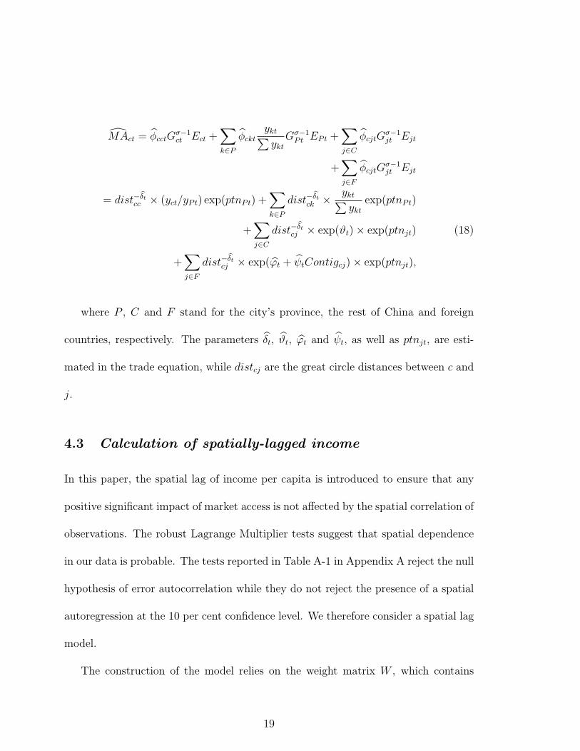
The market access of city c in province P then consists of four parts: local market
access (intra-city demand); provincial market access (rest of the province); national
market access (demand from other Chinese provinces); and world market access.
13 For conciseness, estimates of this trade equation are not shown but are available on request.Our results are in line with those of De Sousa and Poncet (2007) and interested readers are referredto this paper for more details.
18
MAct = φcctGσ−1ct Ect +
∑k∈P
φcktykt∑yktGσ−1Pt EPt +
∑j∈C
φcjtGσ−1jt Ejt
+∑j∈F
φcjtGσ−1jt Ejt
= dist−δtcc × (yct/yPt) exp(ptnPt) +∑k∈P
dist−δtck ×ykt∑ykt
exp(ptnPt)
+∑j∈C
dist−δtcj × exp(ϑt)× exp(ptnjt) (18)
+∑j∈F
dist−δtcj × exp(ϕt + ψtContigcj)× exp(ptnjt),
where P , C and F stand for the city’s province, the rest of China and foreign
countries, respectively. The parameters δt, ϑt, ϕt and ψt, as well as ptnjt, are esti-
mated in the trade equation, while distcj are the great circle distances between c and
j.
4.3 Calculation of spatially-lagged income
In this paper, the spatial lag of income per capita is introduced to ensure that any
positive significant impact of market access is not affected by the spatial correlation of
observations. The robust Lagrange Multiplier tests suggest that spatial dependence
in our data is probable. The tests reported in Table A-1 in Appendix A reject the null
hypothesis of error autocorrelation while they do not reject the presence of a spatial
autoregression at the 10 per cent confidence level. We therefore consider a spatial lag
model.
The construction of the model relies on the weight matrix W , which contains
19
information about the relative dependence between the cities in our sample. The
literature suggests a number of alternative weighting methods. The most widely-used
are based on contiguity and distance between localities, but differ in the particular
functional form retained. As recommended by Anselin and Bera (1998) and Keller
(2002), the elements of the matrix have to be exogenous14, otherwise the empirical
model becomes highly non-linear. We choose a spatial weighting matrix W that
depends exclusively on the geographical distance dcj between cities c and j, since
the exogeneity of distance is absolutely unambiguous. We use the inverse squared
distance in order to reflect a gravity relation. The distance-based weights, wcj, are
thus defined as
wcj = 0, if i = j
wcj = 1/d2cj, if dcj ≤ 800
wcj = 0, if dcj > 800
The distance of 800 km is the cut-off level above which interactions are assumed
to be negligible. This is important since there must be a limit to the range of spatial
dependence allowed by the spatial weights matrix (Abreu et al., 2005).15 We will
check that our results are robust to changes in the cut-off level.
The matrix W is then row-standardized (with w∗cj being an element of the stan-
dardized weight matrix) as w∗cj = wcj/∑
j wcj, so that each row sums to one and each
weight may be interpreted as the city’s share in the total spatial effect.
Using the standardized weight matrix W , our spatially-lagged income variable,
14 This condition is a prerequisite for the introduction of spatial econometrics.15 This is due to the asymptotic property required to obtain consistent estimates of the model
parameters.
20
spatial lag, is then given by Wyct =∑
j 6=c(yjtw∗cj).
16
5 Empirical estimation results
5.1 Benchmark estimates
Having calculated market access at the city level, MAc, and the spatial lag of our
dependent variable, we can now estimate our human-capital augmented version of
the wage equation. Taking the natural logarithms of Equation (13), introducing a
time dimension and controlling for time-invariant city effects, ηc, and common time
effects, λt, yields the following estimation equation:
Our benchmark estimates are obtained using panel regression techniques (city-
level and year fixed effects). We report bootstrap standard errors to control for the
potential econometric problem that arises from the two-step calculation of our market
access variable. This variable is calculated from parameters that are themselves
estimated with standard errors in an initial regression. As a consequence we verified
that our results were robust to the correction of the biased standard errors by applying
the “bootstrap” procedure to each of our regressions.17
Column 1 of Table 1 shows the estimates of Equation (19), which reveal a positive
and significant impact of market access and human capital on per capita income. As
16 While income per capita varies over time, the spatial weight matrix remains unchanged.17 Only Column 8 of of Table 1 does not display bootstrap standard errors.
21
discussed by Head and Mayer (2006), the intercept a depends on the input require-
ment coefficients F and c. These are likely to vary across cities and time due to
differences in capital intensity. As such, from Column 2 onwards, we control for city-
level capital stock and employment, whose estimated parameters are of the expected
sign.
In Column 3, we introduce the spatially-lagged dependent variable, to account
for any spatial dependence in China. As explained above, the spatial lag of income
per capita y in city c corresponds to the sum of spatially-weighted values of y for the
surrounding locations.
The results suggest that spatial dependence between Chinese cities is important
but that it does not alter our estimates of the determinants of city income. The
estimated coefficients on the other explanatory variables are little changed from those
in column 1. Accounting for spatial dependence leads to an increase of one percentage
point in the R2 statistic.
Before looking in detail at the impact of market access, we consider two robustness
checks for our spatial lag variable. As described in Section 3, the variable in Column
3 relies on a cut-off of 800 km. The results with other cut-offs for the spatial lag are
very similar to those in Column 3, as shown in Columns 4 and 5 which are based on
cut-offs of 600 km and 1,200 km, respectively.
Our estimates of the elasticity of city-level per capita income to market access are
robust to the control for spatial dependence in per capita income. This coefficient
of 0.07 is slightly lower than those obtained in province-level data by De Sousa and
22
Poncet (2007), and in individual data by Hering and Poncet (2009).18
Growing differences in trade costs or market size between Chinese cities can there-
fore produce rising income inequality. Our benchmark estimates (Column 3) imply
that the doubling of market access that occurred between 1995 and 2002 would be
associated with a 7 per cent rise in per capita income. The coefficient of 0.2 on
the spatial lag further suggests that changes in this variable between 1995 and 2002
correspond to a rise of 20 per cent in per capita income.
To ensure that our results are reliable, Column 6 introduces population density,
as larger and/or denser cities should benefit more from knowledge spillovers between
firms and workers, leading to greater worker productivity and incomes. The first five
columns did not sufficiently control for this aspect, so significant market access could
reflect a size effect caused by spillovers between firms. The results show that the
impact of MA is slightly reduced when population density is controlled for; this does
not however change the flavor of our results.
We have not as yet addressed the potential simultaneity problem. City fixed
effects control for time-invariant omitted variables, but reverse causality remains an
issue. Market access, as an explanatory variable, is a weighted sum of all potential
expenditures, including local expenditures. These expenditures depend on income,
raising the concern of reverse causality. Since a positive income shock will raise E and
thus MA, we use a two-fold approach to test the robustness of our estimates: we first
estimate our equation in first differences (Column 7); second, we instrument market
access (Column 8). In Hering and Poncet (2009) market access is instrumented by a
18Head and Mayer (2006) find a similar value (0.1) on European data.
23
variable called centrality, which measures the distance of each city in the sample to
the center of every inhabited 1 ◦ by 1 ◦ cell in the world population grid. Here, we
appeal to panel data, so centrality is not a valid instrument for market access, as it
does not vary over time. In Column 8, we thus resort to two instruments which are
inspired by the GMM strategy, even though they significantly reduce our sample size:
the first and second differences in market access. Hansen’s J-test of overidentifying
restrictions does not significantly reject the validity of our instruments. We also report
the Cragg-Donald F-statistic, suggested by Stock and Yogo (2002) as a global test for
weak instruments (i.e. it tests the null hypothesis that a given group of instruments
is weak against the alternative that they are strong). Our instrument set is accepted
as strong, since the Cragg-Donald F-statistic exceeds the critical value of 10 per cent
maximum bias of the IV estimator relative to OLS at the 5 per cent confidence level.
The next step is to carry out the Durbin-Wu-Hausman test, which tests for the
endogeneity of market access in an IV regression. Since this test does not reject the
null hypothesis of exogeneity of market access (at the 10 per cent confidence level),
we report the OLS estimates since they are more efficient than IV estimates (Pagan,
1984). All of the test statistics are displayed at the bottom of Table 1.
5.2
The heterogeneous influence of market access
One novel contribution of this paper is to test whether the relationship between
market access and income depends on city characteristics. It is likely that the con-
tribution of market access to income inequality in China is rooted in not only the
24
heterogeneity of market access across cities but also the heterogenous impact of mar-
ket access on income, depending on city characteristics, and notably immigration
intensity.
According to our theoretical model, in the case of quasi-infinite labor supply for
the manufacturing sector, wages will respond only little to changes in demand from
international and local markets. This relates to the two different mechanisms by
which the local economy can adjust to a change in the demand for its goods: either
quantitative adjustment with new workers filling positions to answer the additional
demand, or, in the case of insufficient labor mobility, adjustment takes the form of a
change in prices, so that income rises with market access.
To see whether the impact of market access depends on immigration intensity, we
consider two sub-samples: high- and low-immigration cities. The immigration rate
used to make this distinction is taken from the 2000 population census, and is calcu-
lated as the ratio of incoming population with household registration in another city
or county of the same province or another province over the city’s total population.
For cities with above-median immigration the “High immigration” dummy equals 1;
those below the median are classified as low immigration.
Column 1 interacts market access with this “High immigration” dummy, while
columns 2 and 3 run separate regressions for high- and low-immigration cities. Our
results are consistent with the predictions: the market-access coefficient is large and
significant at the 1 per cent level in cities with low immigration; in high-immigration
cities, market access has a much smaller effect, as shown by the negative and signif-
icant coefficient on the interaction term in Column 1 and the coefficients on market
25
access in Column 2 and 3. According to these estimates, a doubling of market access
is associated with a 11 per cent rise in income in low-immigration locations, compared
to a 3 per cent rise in high-immigration locations. Our results are in line with those in
Hering and Poncet (2009), who noted, using individual wage data, a greater effect of
market access on the wages of skilled workers. They argue that high-skilled workers
are likely to benefit more from market access as they are less at risk from migrants,
who are in the majority low skilled.
No such heterogeneity results when economic development (instead of migration)
is used to differentiate cities.19 Given the insignificant interaction term of market
access and the level of income per capita in Column 4, the impact of market access
does not seem to be significantly different between these two groups.
5.3 What lies behind spatial dependence?
So far, we have only established that spatial dependence plays a role in determining
the spatial distribution of income within China. The next step is to understand what
lies behind this effect.
We have already taken the demand side into account via market access, so the
significant spatial lag effect must reflect something other than pure demand. Two
potential candidates are technology and knowledge spillovers. To check this hypoth-
esis, we see whether the impact of spatial lags is stronger in environments which are
more favorable to the exchange of ideas and factors.
We use two proxies for the ease of communication between neighboring cities: the
19 We choose income per capita in 1990 as the criterion to split the sample.
26
rate of intra-provincial migration and the quality of the surrounding infrastructure.
As in the previous section, we create two dummy variables, “High internal migration”
and “Good surrounding infrastructure”, that we interact with the spatial lag.
As before, we use migration data from the 2000 population census, which dis-
tinguishes between migrants coming from the same province and those coming from
other provinces. High internal immigration cities are those where the percentage of
population coming from a different location within the same province is above the
median.
To see whether a city is surrounded by good infrastructure we calculate the spatial
lag of the variable “density of streets”.20 “Good surrounding infrastructure” cities
have values of this spatial lag of infrastructure above the median.
Both variables, intra-provincial migration and the spatial lag of infrastructure,
reflect the mobility of factors and goods between closely located cities. We imagine
that spatial dependence may have a stronger impact in regions with greater labor
mobility. First, with greater mobility, wages in one location will move in line with
wages in surrounding cities, to avoid losing workers to neighbors. Second, migration
creates spillovers. Migrants from more productive cities bring knowledge with them
which may well improve productivity in the immigration location. Last, a city that is
known to accept migrants and offer job opportunities might attract qualified migrants
and consequently increase productivity and income.
A well-developed infrastructure facilitates communication and commuting be-
20 As for the spatially-lagged income variable, we weigh the density of streets (with respect topopulation) of each neighboring city by the bilateral distance.
27
tween cities and therefore knowledge transfers and spillovers. Fewer impediments
to the exchange of factors and goods will intensify the competition between cities and
may bid up the price of labor in order to attract the required work force.
We thus expect the interaction terms, introduced in Columns 5 and 6, to be
positive, reinforcing the spatial lag variable. This is indeed the case. The interac-
tions of the spatial lag with both “High internal migration” and “Good surrounding
infrastructure” are positive and significant.
The last column includes both interactions of the spatial lag as well as the in-
teraction of market access with “High Immigration”. All three of the interactions
are significant. The coefficient of the original spatially-lagged income is now much
reduced. The impact of neighboring cities is therefore at least partly due to migration
and its associated spillovers.
6 Conclusion
This paper has examined the role of economic geography and spatial dependence
in explaining the spatial structure of per capita income in China. Our econometric
specification relates city-level per capita income to a transport-cost weighted sum of
demand in surrounding locations after controlling for spatial dependence and endow-
ments. The data come from a sample of 194 Chinese cities between 1995 and 2002.
We find that per capita income has increased due to both better market access and
the reinforcement of spatial interdependence between Chinese cities.
This effect of market access on income inequality depends on local immigration
28
intensity. The elasticity of income to market access is much higher in cities located in
provinces which are characterized by lower immigration. While further international
trade integration of China is expected to fuel an upward pressure on wages, this can be
mitigated by lower barriers to internal migration. In the light of this complementarity,
further liberalization of internal migration may help to maintain the Chinese price
competitiveness. These results confirm those in previous work (De Sousa and Poncet,
2007; Hering and Poncet, 2009).
We also find heterogeneity in the impact of spatially-lagged income, which has a
stronger influence in cities with a higher percentage of intra-provincial migrants or
which are surrounded by good infrastructure. This suggests that neighboring cities
have a greater impact when the mobility of factors and goods is facilitated. In this
case, knowledge spreads more easily and competition for workers is fiercer, increasing
the city’s income.
29
Table 1: Benchmark estimations. Dependent variable: per capita income
(1) (2) (3) (4) (5) (6) (7) (8)All All All 600 km 1200 km All 1st Diff IV
Spatial lag 0.21∗∗ 0.21∗∗∗ 0.23∗∗ 0.24∗∗ 0.15∗∗ 0.28∗∗∗
(0.10) (0.09) (0.10) (0.10) (0.07) (0.08)
Density 0.14∗∗∗
(0.02)
Year fixed effects Yes Yes Yes Yes Yes Yes Yes YesCity fixed effects Yes Yes Yes Yes Yes Yes no YesObservations 1437 1437 1437 1437 1437 1437 1241 1081R2 0.75 0.76 0.76 0.76 0.76 0.78 0.16 0.68Number of cities 194 194 194 194 194 194 188Hansen J statistic (Prob>F) 1.07 (0.3)Durbin-Wu-Hausman stat (Prob>F) 2.2 (0.14)Cragg-Donald F stat 529.94Critical value (10%) 19.93Bootstrap heteroskedastic-consistent standard errors in parentheses, with ∗∗∗,∗∗ and ∗ denoting significance at the 1,5 and 10 per cent levels respectively. Standard errors are corrected for clustering at the province level. The reportedR-squared is the Within R-squared, which indicates how much of the variation of wages within the group of sectorsis explained by our regressors. The critical value for the Cragg-Donald test is based on a 10 per cent 2SLS bias atthe 5 per cent significance level (see Stock and Yogo, 2002).
30
Table 2: Heterogeneity depending on city characteristics
(1) (2) (3) (4) (5) (6) (7)All High Low All All All All
Year fixed effects Yes Yes Yes Yes Yes Yes YesCity fixed effects Yes Yes Yes Yes Yes Yes YesObservations 1437 716 721 1437 1437 1437 1437R2 0.76 0.82 0.72 0.76 0.76 0.76 0.77Number of cities 194 96 98 194 194 194 194Bootstrap heteroskedastic-consistent standard errors in parentheses, with ∗∗∗,∗∗ and ∗ denoting significance at the 1,5 and 10 per cent levels respectively. Standard errors are corrected for clustering at the province level. The reportedR-squared is the Within R-squared, which indicates how much of the variation of wages within the group of sectorsis explained by our regressors.
Correlation between income p.c. and market access (1995)
Correlation between income p.c. and the spatial lag (1995)
Correlation between income p.c. in 1995 and
its growth rate between 1995 and 2002
89
1011
12ln
(inco
me
p.c.
)
12 13 14 15 16 17ln(market access)
89
1011
12ln
(inco
me
p.c.
)
8 10spatial lag of income p.c.
-3-2
-10
1ln
(gro
wth
rate
of i
ncom
e p.
c. b
etw
een
1995
and
200
2)
8 9 10 11 12ln(income p.c. in 1995)
34
APPENDIX C: Trade data
Trade equation estimations are carried out using trade flows from different sources to cover (i)
intra-provincial (or intra-national), (ii) inter-provincial and (iii) international flows. Chinese and
international trade flows are all merged into one single data set which allows us to calculate the
market capacities of provinces and foreign countries based on their exports to all destinations (both
domestic and international).
C.1. International Data
International trade flows are expressed in current USD and come from IMF Direction of Trade
Statistics (DOTS).
Intra-national trade flows are expressed in current USD and are calculated as the difference
between domestic primary- and secondary-sector production minus exports. Production data for
OECD countries come from the OECD STAN database. For other countries, the ratios of industrial
and agricultural output as a percentage of GDP are extracted from Datastream. These are then
multiplied by country GDP (in current USD) from World Development Indicators 2005.
C.2 Chinese Data
Provincial foreign trade data are obtained from the Customs General Administration database,
which records the value of all import and export transactions which pass via Customs. Provincial
imports and exports are decomposed into those concerning up to 230 international partners. This
database has previously been discussed by Lin (2005) and Feenstra, Hai, Woo and Yao (1998).
The exchange rate is the average exchange rate of the Yuan against the US dollar in the China
Exchange Market. This comes from the China Statistical Yearbook.
Intra-provincial flows or foreign intra-national flows, i.e. exports to itself, are computed fol-
lowing Wei (1996) as domestic production minus exports. Production data for Chinese provinces
are calculated as the sum of industrial and agricultural output. Output in yuan are converted into
current USD using the annual exchange rate. All statistics come from China Statistical Yearbooks.
35
Inter-provincial trade is computed as trade flows with the rest of China. Provincial input-output
tables21 provide the decomposition of provincial output, and the international and domestic trade
of tradable goods. These are available for 28 provinces, with data missing for Tibet, Hainan and
Chongqing.
7 References
Abreu M., H. De Groot, and R. Florax, (2005), ‘Space and Growth: A Survey ofEmpirical Evidence and Methods’, Region et Developpement 21, 13-44.
Anselin L., and A. Bera, (1998), ‘Spatial Dependence in Linear Regression Modelswith an Introduction to Spatial Econometrics’, in Handbook of Applied Eco-nomic Statistics, Ullah A, Giles DEA (eds). (Berlin: Springer-Verlag).
Au C.-C., and V. Henderson, (2006), ‘How Migration Restrictions Limit Agglom-eration and Productivity in China,’ Journal of Development Economics, 80:2,350-388.
Baldwin R., R. Forslid, P. Martin, G. Ottaviano, and F. Robert-Nicoud, (2003), Eco-nomic Geography and Public Policy, (Princeton: Princeton University Press).
Blonigen B. A., R. B. Davies, G. R. Waddell, and H. Naughton, (2007), ‘FDI inSpace: Spatial Autoregressive Relationships in Foreign Direct Investment’, Eu-ropean Economic Review 51:5, 1303-1325.
Breinlich H., (2006), ‘The Spatial Income Structure in the European Union - WhatRole for Economic Geography?’, Journal of Economic Geography 6:5, 593-617.
Buettner T., (1999), ‘The effects of unemployment, aggregate wages, and spatialcontiguity on local wages: An investigation with German district level data’,Papers in Regional Science 78, 47-67.
Cheung K. and P. Lin, (2004), ‘Spillover Effects of FDI on Innovation in China:Evidence from the Provincial Data’, China Economic Review 15:1, 25-44.
21Most Chinese provinces produced square input-output tables for 1997. A few of these arepublished in provincial statistical yearbooks. We obtained access to the final-demand columnsof these matrices from the input-output division of China’s National Bureau of Statistics. Ourestimations assume that the share of domestic trade flows (that is between each province and therest of China) in total provincial trade is constant over time.
36
Combes P.-P., G. Duranton and L. Gobillon, (2008), ‘Spatial Wage Disparities:Sorting Matters!,’ Journal of Urban Economics, 63:2, 723-742.
Coughlin C. C., and E. Segev, (2000), ‘Foreign Direct Investment in China: A SpatialEconometric Study’, The World Economy 23:1, 1-23.
De Sousa J., and S. Poncet, (2007), ‘How are wages set in Beijing?’, CEPII, workingpaper, 2007-13.
Hanson G. H., (2005), ‘Market Potential, Increasing Returns, and Geographic Con-centration’, Journal of International Economics 67:1, 1-24.
Head K., and T. Mayer, (2006), ‘Regional Wage and Employment Responses toMarket Potential in the EU,’ Regional Science and Urban Economics, 36(5),573-594.
Hering L. and S. Poncet, (2009), ‘Market access and individual wages: evidence fromChina’, Review of Economics and Statistics, forthcoming.
Fingleton B., (1999), ‘Estimates of Time to Economic Convergence: An Analysis ofRegions of the European Union’, International Regional Science Review 22(1):5-34.
Fingleton B., (2006), ‘The new economic geography versus urban economics: anevaluation using local wage rates in Great Britain’, Oxford Economic Papers56(3): 501-530.
Fujita M., P. Krugman, and A. J. Venables, (1999), The Spatial Economy: Cities,Regions and International Trade, (MIT Press, Cambridge MA).
Keller W., (2002), ‘Geographic Localization of International Technology Diffusion’,American Economic Review 92: 120-142.
Krugman P. and A. J. Venables, (1995), ‘Globalization and the Inequality of Na-tions’, Quarterly Journal of Economics, 110(4), 857-880.
Lin S., (2005), ‘Geographic Location, Trade and Income Inequality in China’, in R.Kabur and A. J. Venables Spatial (eds.) Inequality and Development, (OxfordUniversity Press, London).
Madariaga, N. and S. Poncet, (2007), ‘FDI in China: spillovers and impact ongrowth’, The World Economy 30, 837-862.
Ma A. C., (2006), ‘Geographical Location of Foreign Direct Investment and WageInequality in China’, The World Economy 29:8, 1031-1055.
37
Meng X., R. Gregory, and Y. Wang, (2005), ‘Poverty, Inequality and Growth inUrban China, 1986-2000’, Journal of Comparative Economics 33:4, 710-729.
Mion G., (2004), ‘Spatial externalities and empirical analysis: the case of Italy’,Journal of Urban Economics 56, 97-118.
Pagan A., (1984), ‘Model Evaluation by Variable Addition’, in D.F. Hendry andK.F. Wallis (eds) Econometrics and Quantitative Economics, Blackwell: Ox-ford, chapter 5, 103-134.
Redding S. J., and A. J. Venables, (2004), ‘Economic Geography and InternationalInequality’, Journal of International Economics 62:1, 53-82.
Rey S., and B. Montouri, (1999), ‘U.S. Regional Income Convergence: A SpatialEconometric Perspective’, Regional Studies 33, 145-156.
Stock J. H. and M. Yogo, (2002), ‘Testing for weak instruments in linear IV regres-sion’, NBER technical working paper 284.
Tobler W. R., (1970), ‘A Computer movie simulating urban growth in the DetroitRegion’, Economic Geography 46, 234-240.
Wei S.-J., (1996), ‘Intra-National Versus International Trade: How Stubborn AreNations in Global Integration’, NBER Working Paper 5531.
Ying L. G., (2003), ‘Understanding China’s recent growth experience: A spatialeconometric perspective’, The Annals of Regional Science, 37:4, 613-628.