See discussions, stats, and author profiles for this publication at: https://www.researchgate.net/publication/227354394 Income, Relational Goods and Happiness Article in Applied Economics · February 2011 DOI: 10.1080/00036840802570439 · Source: RePEc CITATIONS 69 READS 894 3 authors: Some of the authors of this publication are also working on these related projects: Economic Growth, Population Dynamics, and Sustainability View project Monetary Analysis and Macroeconomic Modelling, New insights for the understanding of finance Etapa I View project Giovanni Trovato University of Rome Tor Vergata 51 PUBLICATIONS 1,049 CITATIONS SEE PROFILE Leonardo Becchetti University of Rome Tor Vergata 356 PUBLICATIONS 5,527 CITATIONS SEE PROFILE David Andres Londono-Bedoya Pontificia Universidad Javeriana 19 PUBLICATIONS 304 CITATIONS SEE PROFILE All content following this page was uploaded by David Andres Londono-Bedoya on 15 May 2014. The user has requested enhancement of the downloaded file.
Transcript
See discussions, stats, and author profiles for this publication at: https://www.researchgate.net/publication/227354394
Income, Relational Goods and Happiness
Article in Applied Economics · February 2011
DOI: 10.1080/00036840802570439 · Source: RePEc
CITATIONS
69READS
894
3 authors:
Some of the authors of this publication are also working on these related projects:
Economic Growth, Population Dynamics, and Sustainability View project
Monetary Analysis and Macroeconomic Modelling, New insights for the understanding of finance Etapa I View project
Giovanni Trovato
University of Rome Tor Vergata
51 PUBLICATIONS 1,049 CITATIONS
SEE PROFILE
Leonardo Becchetti
University of Rome Tor Vergata
356 PUBLICATIONS 5,527 CITATIONS
SEE PROFILE
David Andres Londono-Bedoya
Pontificia Universidad Javeriana
19 PUBLICATIONS 304 CITATIONS
SEE PROFILE
All content following this page was uploaded by David Andres Londono-Bedoya on 15 May 2014.
The user has requested enhancement of the downloaded file.
Complete List of Authors: Becchetti, Leonardo; University of Rome Tor Vergata, Economia e Istituzioni<br>Trovato, Giovanni; University of Rome Tor Vergata, Economia e Istituzioni<br>Londono Bedoya, David Andres; University of Rome Tor Vergata, Economia e Istituzioni; University of Rome Tor Vergata, Faculty of Economics
JEL Code:
D60 - General < D6 - Welfare Economics < D - Microeconomics, I31 - General Welfare|Basic Needs|Living Standards|Quality of Life < I3 - Welfare and Poverty < I - Health, Education, and Welfare
Editorial Office, Dept of Economics, Warwick University, Coventry CV4 7AL, UK
Submitted Manuscript
For Peer ReviewIncome, Relational Goods and Happiness
Abstract
Our empirical analysis on the determinants of self declared happiness on more than100,000 individuals from representative samples in 82 world countries does not reject thehypothesis that the time spent for relationships has a significant and positive impact onhappiness. This basic nexus helps to understand new unexplored paths in the so called“happiness-income paradox”. To illustrate them we show that personal income has twomain effects on happiness. The first is a positive effect which depends on individual’sranking within domestic income quintiles. The second is determined by the relationshipbetween income and relational goods. In principle, more productive individuals may sub-stitute (if the income effect prevails over the substitution effect) worked hours with thenonworking time made free for enjoying relationships, when they have strong preferencesfor them. The problem is that these individuals tend to have ties with their income classpeers who share with them a high opportunity cost for the time spent for relationships.Hence, a coordination failure may reduce the joint investment in relational goods (localpublic goods which need to be co-produced in order to be enjoyed together) and, throughthis effect, individuals in the highest income quintiles may end up with poorer relationalgoods. The indirect impact of personal income on happiness through this channel is there-fore expected to be negative.Keywords: happiness, relative income, relational goods.JEL:D60,I31, 030
1 Introduction
Economic policy prescriptions always imply an explicit or implicit ranking of priorities in-corporated into a specific welfare function, which has to be maximised under given resourceconstraints.
The ultimate criteria to define such priorities should be based on the knowledge of factorsdetermining human happiness (or life satisfaction), since the latter ought to be the ultimategoal of national and international policymakers’ action.
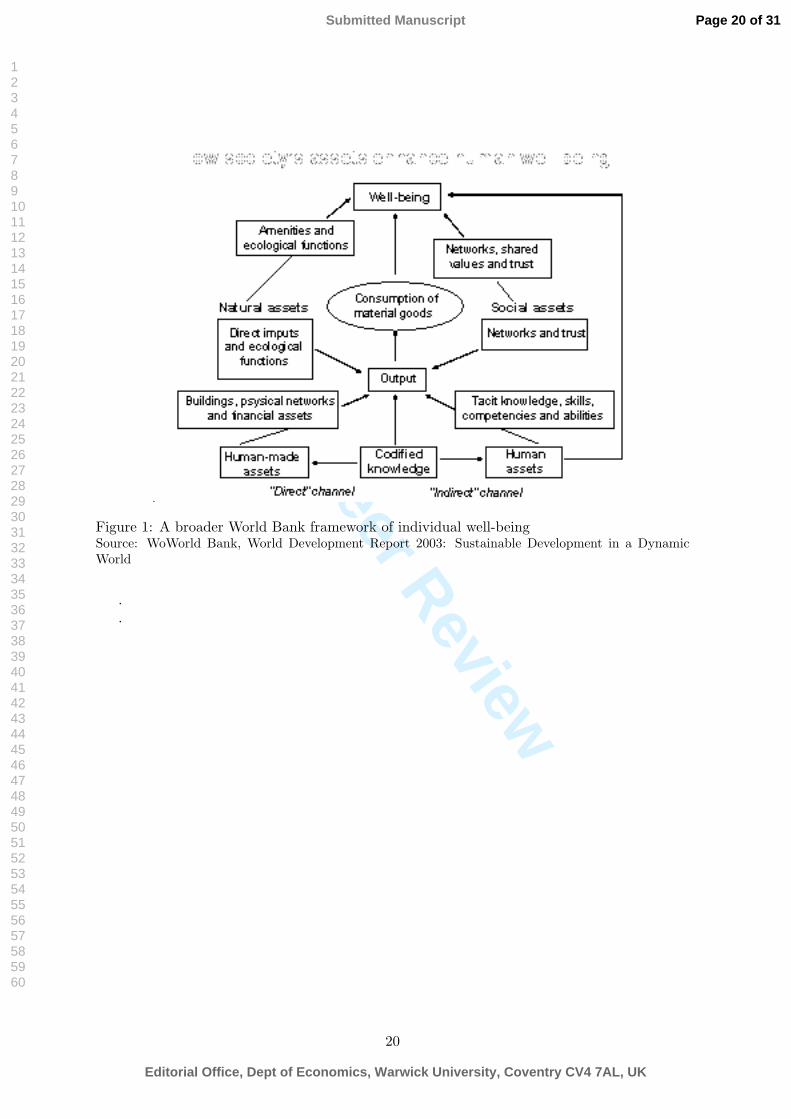
The 2003 World Bank development report clearly outlines a broad framework for humanwellbeing which could inspire policymakers prescriptions along this line (see Figure 1). Insuch framework it is acknowledged that (in addition to income enabled consumption) human,environmental and social resources are factors which, beyond their role as production inputs,have in themselves, through their direct fruition, a positive impact on individual happiness.
If the World Bank welfare conception is a good description of the reality of the humanwellbeing, we expect education and quality of social ties to have significant and positive effectson happiness, independently from their expected contribution to individual productivity andincome. While the impact of education on individual wellbeing has been thoroughly explored
1
Page 1 of 31
Editorial Office, Dept of Economics, Warwick University, Coventry CV4 7AL, UK
in the empirical literature (Becker et al., 1997), evidence on the impact of relational goods1 is,to our knowledge, very scarce.
Several other reasons of interest exist, beyond the lack of empirical work, to focus ourresearch effort on the nexus between relational goods and happiness.
First, the exploration of non monetary causes of happiness is not to be considered out-side the realm of economic analysis, as it may be of great importance in understanding thedeeper motivation of human economic behaviour including consumption, productivity and en-trepreneurship.
The acknowledgement of the importance of the investigation on the wealth-happiness nexusgoes back to Malthus (1798), 2Marshall (1890), Veblen (1899), Dusenberry (1949) and Hirsch(1976). In extreme synthesis, these authors remember that the nexus between the mean(wealth) and the end of any human existence (happiness) is the most important field of inves-tigation for a social scientist.
Second, growth oriented policy measures, which do not take into account their eventualunintended consequences on non monetary factors affecting individual happiness, may achievetheir primary goal (economic growth), but may miss the target of consolidating political con-sensus if they generate undesirable negative effects on happiness.3
The recognition of the relevance for economic policies of the research on the determinantsof happiness does not imply a positive judgement on its feasibility.
One of the leading criticisms on this point is set forth by the approach which argues thatempirical analyses should be carried out only on revealed preferences. This approach regardssubjective utility as non scientific since it is not objectively measurable (Frey and Stutzer,2002a).
On this point Frey and Stuzter (2002a) nicely reports Sen’s (1986) sentence on the factthat “the popularity of the positivistic view is due to a mixture of an obsessive concern withobservability and a peculiar belief that choice...is the only human aspect that can be observed”and provide several examples of nonobjectivist analyses such as theoretical studies on emotions(Elster, 1998), self signalling, goal completion mastery and meaning (Lowenstein, 1999) andstatus (Frank, 1985).
Another advantage of happiness studies with respect to analyses based on revealed prefer-ences is that the same consumption bundle may lead to completely different levels of satisfactionaccording to the complex pattern of intrinsic and extrinsic motivations and to the course ofaction which led to obtain such material outcome. This argument may be resumed by arguingthat ”experience utility” is at least as relevant as ”choice utility”. In this sense the empir-ical research on the determinants of happiness overcomes the ”consequentialist” assumptionthat selected strategies and experience lived during the course of actions have no effects onindividual happiness beyond the realized outcome.
The main arguments in defence of the reliability of data on self declared happiness are:1Beyond the detailed evidence on the effects on happiness of marital status (Argyle, 1999; Blanchflower-
Oswald, 2004; Frey-Stutzer, 2006, 2002a, 2002b; Johnson-Wu, 2002), which has obviously to do with relationalgoods, there is no investigation, to our knowledge, on the impact of the time spent with different types of friends(working colleagues, co-members of sport and religious associations, etc.).
2An example of it is this nice quote from Malthus (1798) on Adam Smith work: The professed object of Dr.Adam Smiths inquiry is the nature and the causes of the wealth of nations. There is another inquiry, however,perhaps still more interesting, which he occasionally mixes with it, I mean an inquiry into the causes whichaffect the happiness of nations .
3An interesting example of the potential paradoxical adverse effects on happiness of growth oriented policiesis provided by the identification of ”frustrated achievers” (individuals registering positive changes in income andnegative changes in happiness) (see, among others, Graham 2003 and Graham and Pettinato 2005).
2
Page 2 of 31
Editorial Office, Dept of Economics, Warwick University, Coventry CV4 7AL, UK
i) their capacity of passing cultural Darwinian selection in psychology and sociology (Alesina,Di Tella and MacCulloch, 2004); ii) the positive link between self declared happiness andhealthy physical reactions such as smiling attitudes (Pavot 1991, Eckman et al., 1990), heartrate and blood pressure responses to stress (Mayman and Manis, 1993); iii) the link betweenpositive feelings and physical measures of brain activity (higher alfa power in the left parefrontalcortex), with measures of hedonic well being such as life satisfaction being also related withthe same activity (Sutton and Davidson, 1997); iv)the prediction capacity of self declaredhappiness with individuals choosing to discontinue activities associated with low levels of well-being (Kahneman et al., 1993; Frijters, 2000; and Shiv and Huber, 2000); v) the correspondencebetween happiness scores provided by family and friends on the respondent and the respondentown report (see Sandvik et al., 1993; Diener and Lucas, 1999)
Our belief on the validity of the above mentioned arguments, and the importance of ex-tending our knowledge into these new areas, motivates our paper.
The paper is divided into seven sections (including introduction and conclusions). In thesecond section we present a short survey on the nexus among income, relational goods andhappiness in two steps. First, we explore the direct link between each of the first two variablesand happiness. Second, we investigate the complex nexus among the three, which includesan indirect effect of income on happiness, through the impact that the first variable has onrelational goods. In this part of the second section we formulate our hypothesis on direct andindirect effects of income on happiness, and on the direct effect of the intensity and time spentin relational goods on happiness itself. The hypothesis will be tested in the empirical analysis.In the third section we present descriptive evidence on the positive link between income andhappiness, time spent for relational goods and happiness, and on the nonpositive relationshipbetween income and time spent for relational goods.
In the fourth section we test our hypotheses on the above mentioned links and test the ro-bustness of our findings to different (gender, geographical area, religious affiliation) subsamplesplits.
2 Income, relational goods and happiness: the theoretical lit-erature
2.1 Income and happiness
The empirical literature on the determinants of happiness, even though at its infant stage,includes many relevant contributions.
A dominant field of inquiry studies the impact of levels and changes in income on perceivedhappiness. Aspects such as those of the impact of marital relationship, education, healthstatus, and dynamic effects of changes of these variables on self declared happiness, have alsobeen extensively investigated. 4Finally, the effects of country specific economic variables, suchas employment and inflation, have also been explored (Clark and Oswald, 1994; Gallie andRussel, 1998; Di Tella, MacCulloch and Oswald, 2001 and 2003).
4A general problem in this literature is the scarcity of panel data in which self declared happiness in differentyears is reported for the same individuals. The most relevant exceptions are the German socioeconomic panel(GSOEP)and the British Household Panel Survey (BHPS). Empirical research on panel data generally evidencesthe presence of biunivocal causality relationships where changes in a given factor (income, health, family oremployment status) affects happiness but inherited traits captured by fixed effect are related to individualhappiness and in turn may significantly affect changes in the above mentioned variables. For a detailed surveyon these issues see Clark et al., 2006)
3
Page 3 of 31
Editorial Office, Dept of Economics, Warwick University, Coventry CV4 7AL, UK
Some of these empirical studies have clearly evidenced the existence of what is sometimescalled the happiness-income puzzle. The puzzle originates from the famous Easterlin (1974 and2001) contributions in which the dramatic growth in per capita GDP in post war US is com-pared with a stagnating or slightly declining self declared happiness. It seems confirmed whenwe compare happiness across countries and observe that the income per capita divide betweendeveloped and developing countries is not reflected into equivalent differences in self reportedhappiness. On this point, it is well known that the comparison of levels of happiness acrosscountries is subject to severe methodological problems, such as cultural differences in the wayhappiness is self reported and problems arising from cardinal comparisons of happiness levels.It is also valid the remark of Sen (2005) arguing that happiness studies should not fall intothe trap of considering subjective happiness as the only value, thereby implicitly legitimatingexploitation and poor living conditions in those cases in which they lead to adaptation of thehuman being to misery. Nonetheless, it is evident that the observation of average happinesslevels in less developed countries, which are almost equal to those of rich countries, must leadus to explore more in depth the puzzle of the relationship between income and happiness.
A first tentative partial explanation of this puzzle is based on the conception of income asa positional good (Hirsch, 1976). Under this perspective, the relative income effect dominatesthe absolute one and the positive impact of income on happiness may be partially offset bythe negative externalities arising from an unfavourable position in terms of relative incomein one’s own reference group.5 A second rationale hinges on the so called adaptation theory.According to it, the achievement of a target (a certain level of income) raises new expectations,thereby creating a gap between increased individual income targets and the achieved level ofincome, which also reduces the perceived happiness arising from past endeavours (Easterlin,2001). A more extreme perspective, represented by the so called set point theory (Costa etal., 1987; Cummins et al., 2004),6 establishes that any positive change in income (as of anyother event in life) has no permanent effects on happiness, the latter being uniquely determinedby individual temperament. A fourth argument, provided by Scitowsky (1996), is based onthe conflict between comfort and stimulation. Under certain conditions higher income maygenerate more comfort and dampen stimulation for new endeavours. This may seriously reducethe expected positive effect of income on happiness.
In spite of all these dampening effects which may help to illustrate the puzzle of the de-creasing marginal effect of income on happiness and of the reduced happiness gap betweenhigh income and non high income countries, we must not neglect that the positive relationshipbetween income and happiness seems to be robust and supported in different countries andsample periods (see, among others, Easterlin, 1995 and 2000; Frey and Stutzer, 2000; Di Tella,Mc Culloch and Oswald, 2000).
2.2 Relational goods and happiness: the fellow feelings hypothesis
Our argument is that the overall pattern of the effects of income on happiness may be under-stood and explored only if we bring into the field the complex link among income, relationalgoods and happiness. To investigate the nexus among these three variables we first need to
5Support for the relative income hypothesis may be found in several papers starting from the seminal con-tribution of Dusenberry (1949), up to the more recent contributions of Frank (2005) and Layard (2005).
6Easterlin (2004) correctly arguments that, if public policies have the goal of improving individual well being,the set point theory leads to a nichilist or laissez faire view since any change in happiness determinants has nopermanent effects on individual happiness, the latter being solely determined by individual temperament andgenetic endowments.
4
Page 4 of 31
Editorial Office, Dept of Economics, Warwick University, Coventry CV4 7AL, UK
analyse the direct relationship between relational goods and happiness.Standard microeconomic foundations of individual’s utility usually neglect the fact that
the latter does not depend only on the amount of consumed goods, but also on the relationalcontext in which material goods are consumed (eating a pizza alone is not the same as eating apizza with friends). Most of the times the effect of the relational context on utility dominatesby far that of the consumed material goods. With a nice example, Gui (2000) arguments thatthe enjoyment arising from a hairdresser’s cut largely depends on the friendly environment ofthe shop and would be greatly reduced if the cut were to be done by an automatic machineon customers sitting in isolated boots. According to Gui (2002) and Uhlaner (1989), rela-tional goods are local public goods which are co-produced and co-consumed by agents duringtheir economic transactions. Bruni and Stanca (2005) argue that personality and absence ofinstrumental motivations are key elements affecting the quality of relational goods and thatthe economic literature on the role of sociality on happiness is paralleled by several contri-butions from psychologists on the crucial importance of “relatedness” as a basic human need(Baumeister and Leary, 1995, Deci and Ryan, 2001)
Going back to the history of economic thought, one of the nicest and insightful interpre-tations of the link between social ties and happiness is provided by Adam Smith (1759) withhis well known theory of fellow feelings. In the “Theory of moral sentiments” Smith arguesthat the effect of relational goods on happiness is increasing in i) the amount of time andexperiences that two individuals have lived together and have shared in the past and ii) theircommon consent, with the former significantly affecting the latter.7 The related hypothesisstemming from Adam Smith’s theory is that there are warmer (family, close friends, membersof religious associations for believers) and, presumably, colder (working colleagues, sport com-panions) relationships, with the former having a higher impact on happiness. This hypothesiswill be tested in our empirical analysis.
2.3 Relational goods and happiness: the income crowding out hypothesis
An additional important argument on the relational goods-income-happiness nexus - set forthby several authors but not empirically tested - is that relatively higher income may crowd outthe time spent for relationship, thereby generating an indirect negative effect of income onhappiness.
The nexus among the three variables is explained in different ways. According to Easterlin(1974), individuals invest too much in the pursuit of higher income underestimating the nega-tive effects on happiness of factors associated to material goods, such as negative externalitiesdepending on relative income and hedonic adaptation. Similar explanations are proposed byPugno (2004) and Bartolini et al. (2002), respectively focusing on the effects of the rise ofmaterialistic culture, and of an aggregate rise of income, on the gap between desired and re-alised levels of income which induces individuals to increase working hours, thereby crowdingout relational time.
The unpleasant assumption implicit in these rationales is that individuals are not rationaland affected by a misperception. An alternative hypothesis which does not abstract from in-dividual rationality is provided by Becchetti and Santoro (2004). The two authors considerthat relational goods need to be jointly produced. As far as individuals become more produc-
7An acute observation of Smith is that fellow feelings may be equally fuelled by pleasant and unpleasantjoint experiences and that non physically painful, but emotionally unpleasant, joint experiences have a strongimpact on the formation of a common consent among people. A typical example may be the attendance of afuneral which strengthens solidarity and friendship ties among participants.
5
Page 5 of 31
Editorial Office, Dept of Economics, Warwick University, Coventry CV4 7AL, UK
tive, the opportunity cost of their time spent investing in relational goods becomes higher. Ifthey had simply to decide between working time and leisure, substitution and income effectsshould act in such a way that, if individuals have strong preferences for relational leisure, thelatter may actually turn out to be higher and not lower, after an increase in productivity. Theproblem with relational goods, though, is that they require a joint coordinated investment. Toprovide two simple examples, a marriage is not successful without the coordinated effort of thetwo partners, or, a non professional football match cannot be played if 22 individuals do notdecide jointly to invest some of their time in playing the game, since the absence of only one(or a few) of them may prevent the “production” of this relational good.
Hence, even though one of the individuals investing into the relational good may regard it asa non inferior good (or, even though, for him, the income effect may more than compensate thesubstitution effect), the same individual ends up being less happy, and without relational good,if some of his partners, who must cooperate with him in producing the good, decide differently.The model therefore predicts that coordination failures in the investment on relational goodsmay lead to the paradox that, as far as productivity grows, fully rational individuals maybecome richer in income, but poorer in relational goods, with the latter effect having a negativeimpact on their happiness.
To sketch the theoretical framework behind our reasoning consider the i-th individual withthe following “happiness” function
Hi = f(αi ◦ (Ci − C), βi ◦ lri ,m∑
j=1
γij ◦Xij) (1)
whose separable arguments are the deviation of individual consumption from the medianconsumption of his reference group (Ci − C), relational leisure (lri ) and a series of additional(Xj) factors affecting individual happiness (αi, βi and γi being the weights of such argumentsin individual preferences). The individual faces the following standard time/budget constraintpCi = w[T − tlri ] where w is hourly wage and the opportunity cost of time spent in relationalleisure, T is the total endowment of hours in a given time interval and tlr is the time spent forrelational leisure (i.e. “producing” relational goods)8. Following the literature on relationalgoods we assume that such goods need to be co-produced according to a production functionlr = g(tlri , tlr−i) in which the time spent on relational good by the i-th individual and by hisgroupmate 9are the two inputs which we assume to be linked by some form of complementarity.By replacing the constraint into the happiness function we get
Hi = f
αi ◦
[(T − tlri )wi
P− C
], βi ◦ lri ,
m∑
j=1
γij ◦Xij
(2)
¿From (2) it becomes obvious that the optimal choice of time spent in relational leisure isdriven by the trade off between working less, and investing non working time in the creationof the relational good, and working more to increase individual consumption. Even withoutexplicitly assuming a specific functional form we understand that, in correspondence of theoptimal time spent for relational leisure, the marginal cost of diverting resources from con-sumption via reduced working time must be equal to the marginal benefit generated by theenjoyment of an additional unit of relational good. More formally, if we assume that the
8Non relational leisure is set equal to zero for simplicity.9We assume for simplicity that only two people are needed to produce the relational good.
6
Page 6 of 31
Editorial Office, Dept of Economics, Warwick University, Coventry CV4 7AL, UK
weights of the two arguments are multiplicative and the arguments are separable, we get fromfirst order condition (when maximising with respect to the time invested in relational goods)
∂H
∂tlr= 0 ⇒ α
w
P= β
∂lr
∂tlr(3)
The indirect happiness function must therefore be of the form
V = y
αi
[(T − (tlri )∗)wi
P− C
], βil
ri
[(tlri
)∗,(tlr−i
)∗],
m∑
j=1
γijXij
(4)
where starred variables indicate individually optimal choices of the time spent for relation-ships.
By assuming that richer individuals are also those with higher skills, higher hourly wagesand opportunity cost of leisure, we easily find that they choose in equilibrium a lower amountof time spent for relational leisure. More formally, an increase in the hourly wage (and inthe opportunity cost of time spent for relational leisure) for both individuals has the followingeffects on the indirect happiness function
∂Vi
∂w= y′
{αi
P
[T − tlri − w
∂tlri∂w
]+ βi
∂lri∂tlri
∂tlri∂wi
+ βi∂lri∂tlr−i
∂tlr−i
∂w−i
}(5)
with w = wi = w−i.By assuming that the relational good is co-produced with individuals of the same income
category, we clearly have the case that an increase in productivity (which should correspond toan increase in income under the hypothesis that productivity, wages and income move together)should affect happiness positively (via higher consumption) and negatively (via reduction of theenjoyed relational goods) if one of them or both decide to reduce the investment in relationalgoods.10
3 Empirical findings: descriptive evidence
Our data source is the World Value Survey database, which includes representative samplesfrom 82 countries in the world,11 The World Value Survey presents two questions which aredirectly related to happiness. In the first respondents are asked
“All considered you would say that you are: i) very happy; ii) pretty happy; iii) not toohappy; iv) not at all happy?”.
In the second they are asked “all considered are you satisfied or unsatisfied with your currentlife ?”. The answer to this second question can be given on a scale from 1 (unsatisfied) to 10(fully satisfied).
10Consider that, under the extreme assumption of perfect complements, and when ex ante investment levelsare equal, the decision to reduce investment of just one of the two players automatically reduces the total amountof relational goods to his chosen level of investment.
11The World Values Survey is a worldwide investigation of sociocultural and political change. It has carriedout representative national surveys of the basic values and beliefs of publics in more than 80 countries on allsix inhabited continents, containing almost 80 percent of the world’s population. It builds on the EuropeanValues Surveys, first carried out in 1981. A second wave of surveys, designed for global use, was completed in1990-1991, a third wave was carried out in 1995-1996 and a fourth wave took place in 1999-2001. The surveysare based on stratified, multistage random samples of adult citizens aged 18 and older. Each study containsinformation from interviews conducted with 300 to 4,000 respondents per country.
7
Page 7 of 31
Editorial Office, Dept of Economics, Warwick University, Coventry CV4 7AL, UK
The first question has 112,832 non missing observations, with a tiny share of 3.2 percentof not at all happy people, around 16 percent who declare to be somewhat happy against 53percent quite happy and 27 percent very happy (Table 1). The second question has 117,264non missing observations with 14 percent (5 percent) of respondents indicating the maximumvalue (minimum value) of life satisfaction (Table 2).
If we split the sample into high income OECD countries and the complementary group wefind that happiness is slightly higher in the first group. Very happy people are in fact around33 percent against 25 percent, quite happy 58 percent against 52 percent, somewhat happy 8percent against 20 percent and not at all happy 1 percent against 4 percent.
In the same way the share of respondents to the life satisfaction question indicating themaximum value of 10 in OECD high income countries is around 16 percent against 13 percentin the complementary sample and the share of those placed at the lowest value of this scale is1 percent against 7 percent.
Always on a descriptive point of view, we observe that the relationship between happinessand individual position in domestic income deciles is positive as expected. If we move from thelowest to the highest income quintile the share of not at all happy individuals falls from around18 percent to 11 percent and that of very happy ones grows from 3 to 45 percent (Table 3). Ifwe do the same for the life satisfaction question we find that, when moving from the lowest tothe highest income quintile, the number of those indicating the minimum (maximum) level oflife satisfaction falls from 11 to 2 percent (grows from 14 to 17 percent) (Table 4).
Finally, we investigate the direction of the link between happiness and “relational time” ona descriptive point of view. In the survey we find a series of questions about the time spent:i) with friends; ii) with working colleagues outside the workplace; iii) with relatives; iv) in theworship place (parish, mosque, synagogue) with friends sharing the same religious confession;v) in clubs or volunteering (sport, culture, etc.) association. For each of these questions theanswers can be: i) every week; ii) once or twice a month; iii) a few times per year; iv) never.
The synthesis of this information in a single indicator is problematic. The difference amongintensity modes is not continuous and we decide to aggregate the different ways of spendingtime in relationships.
Our choice is to rank each of the answers on a scale with values which are increasing inthe time spent for relationship (i.e., 3 if the answer is every week and 0 if it is never).12 Wethen average these answers across all the different types of relational time. As a consequence,we obtain a relational indicator with a maximum value of 3, if the respondent spends timeevery week in all the possible modalities and, a minimum value of 0, if he never invest time inrelational goods.
By using this variable we find that the share of very happy (not at all happy) people movesfrom 19 percent (8 percent) when the relational time indicator is lower than 1, to 29 percent(3 percent) when it is higher than 2 (Table 5).
Descriptive evidence therefore outlines a positive relationship between happiness, on theone side, and both progression across income deciles and intensity of relational life, on theother side. But what is the effect of progression across income deciles on relational life ?
Our descriptive findings show that it tends to be inverse U-shaped (Table 6). The share12By looking at the relationship between our indicator and the likely number of times per month spent in
relationship which can be inferred from sample answers we figure out that our scale flattens the presumedfrequency. A robustness check in which we attribute an approximate per month frequency and use the value of4, 1.5 and .3 for the “every week”, “once or twice in a month” and “a few times per year” answers respectively,shows that our findings are substantially unaltered. Results are omitted for reasons of space and available uponrequest.
8
Page 8 of 31
Editorial Office, Dept of Economics, Warwick University, Coventry CV4 7AL, UK
of individuals in the highest income quintiles with a relational time indicator between 2 and 3(dedicating on average more than ”few times in a month” to the different relational activitiesinvestigated in the survey) is around 34.8 percent against that of 37.5 percent for individualsin the third income quintile .13 These descriptive findings provide evidence of a U-shapedrelationship between income and time spent in social ties whose robustness to compositioneffects needs to be verified in the econometric analysis which follows.
4 Empirical findings: econometric evidence
4.1 The single equation estimate
Before describing our specification and commenting our results we share the caveats of Guisoet al. (2003) on the interpretation of findings from this cross-sectional dataset. We agreewith them that what we measure are correlations across variables, without the possibilityof establishing the size and the direction (probably biunivocal) of the causal effects.14 Wetherefore start from the following single equation specification (which is standard in similarstudies) where the direct effects of income and time spent for relational goods on happinessare separately considered.
.The dependent variable (Happyi) takes discrete values from three (very happy) to zero
(not at all happy), Age is the respondent age, introduced in levels and in squares to takeinto account nonlinearities in its relationship with happiness (see, among others, Alesina, 2000and Frey, 2000), Male is a dummy which takes the value of one for men and zero other-wise. To measure the impact of education we include dummies for high school (Mideduc)and (Upeduc) university educational attainment. The job status is measured by two differentvariables (Unempl and Selfempl) recording unemployed and selfemployed individuals respec-tively. We further introduce five family status variables: Numsons (the number of familychildren), Single, Married, Divorced and Separed which are all dummies taking the value ofone if the individual has the given status and zero otherwise.15
We introduce income in two ways. First, we consider a relative income measure by intro-ducing four dummies measuring individual position in the relevant income quintile (DIncome).
13More in detail,if we restrict the indicator to the sum of the time spent in family, with “worship friends” andwith working colleagues, we find that the average value of our relational indicator is 1.47 for the lowest, 1.76for the middle and 1.58 for the highest income quintile. Results are omitted for reasons of space and availableupon request.
14As a partial solution to the problem we propose an estimate with instrumental variables in Table 9 (seesection 4.3) .
15Note that these variables do not sum up to one since the survey reports two additional alternative modalities(unmarried cohabiting partners and widowed).
9
Page 9 of 31
Editorial Office, Dept of Economics, Warwick University, Coventry CV4 7AL, UK
Second, we bring in a continuous measure of (income class median) equivalent income expressedin year 2000 US dollar purchasing power parities in levels and in squares (Eqincome). 16
Finally we introduce our measure of time spent in relationship (Timerel). The constructionof this variable (for which we provided descriptive evidence in Tables 5 and 6) is discussed insection 3.
Among additional controls, we introduce a measure of individual health status.17 Thisvariable is seldom used in the empirical literature, even though it is highly likely to be one ofthe main determinants of people well being.
Our final control is a country measure of economic freedom. To this purpose we use thesynthetic Economic Freedom indicator (for its detailed description see Appendix). Countrydummies are finally added to the covariates set.
Results from this base standard equation are consistent with what found in previous em-pirical research (Tables 7-8, column 1). The male coefficient is negative and significant as inalmost all empirical studies, such as those of Alesina et al. (2000) for US and Europe and Freyet al. (2000) for Switzerland, but differently from what found by Clark and Oswald (1994) inthe UK. Age is inverse U-shaped as in Alesina et al.(2000) and Frey et al. (2000). 18
Both educational variables are positive and significant, consistently with what found inmost of the empirical literature. The significance of education when controlling for measuresof income supports the hypothesis that the benefit of education is not just in the contributionof human capital accumulation to income (returns to schooling). Education is also a goodwhich is enjoyed per se as it enhances human capabilities and functionalities (Sen, 1993). Thisfinding is therefore consistent with the wellbeing scheme of the 2003 WB poverty report (Figure1), in which happiness is related not only to consumption, but also to the direct enjoyment ofeducation.
Results on the marital status are also in line with many literature findings (Argyle 1999,Blanchflower and Oswald, 2003, Frey and Stutzer, 2006, 2002a and b) which evidence a posi-tive impact of marriage and a negative impact of divorce or separation. The relatively highermagnitude of the separation with respect to the divorce coefficient is consistent with the hy-pothesis that negative shocks are partially, but not entirely, reabsorbed. Unfortunately, thequality of our data does not allow us to explore more in depth the difference between divorcedwith and without new relationship and the dynamic of happiness around the marriage event.19
16The World Value Survey database contains two variables which respectively provide the income class andthe median household income value (in local currency) for that class for the majority of countries. For a secondgroup of countries - Azerbaijan, Australia, Belarus, Israel, Armenia, Bangladesh, Belgium, Brazil, Colom-bia, Dominican Republic, Finland, Georgia, Hungary, Indonesia, Iran, Korea, Luxembourg, Nigeria, Pakistan,Philippines, Poland, Puerto Rico, Romania, Tanzania, United Kingdom and Northern Ireland, Viet Nam -the missing median income value has been calculated from World Bank Development Indicators or DomesticAccount data .
17The related question is : “All in all how would you describe your state of health these days ? You wouldsay it is: a) very good; b) good; c) fair; d) poor. We create a categorical variable which takes the value of 3for answer a, 2 for answer b, 1 for answer c and zero for answer d. Robustness checks with slightly differentindicators (i.e. dichotomous with value of one for answers a) and b) and zero otherwise) do not change our mainfindings.
18Unfortunately, we do not dispose of panel data and therefore we cannot say whether our result is due to acohort or a life cycle effect. To this point, a recent work of Easterlin (2005) on individual life cycles shows thatageing is associated to rising income (but to decreasing health) satisfaction.
19Blanchflower and Oswald (2003) find that those remarried are significantly less happy than those in theirfirst marriage. Evidence from Waite et al. (2002) seems to suggest that adaptation to marriage is partial butnot complete so that the latter generates permanent effects on welfare. By commenting these and many otherresults in the literature Frey and Stutzer (2006) find evidence of a biunivocal nexus between happiness andmarriage where education and division of labour within the couple play an important role.
10
Page 10 of 31
Editorial Office, Dept of Economics, Warwick University, Coventry CV4 7AL, UK
Findings on the impact of marital status on happiness are not at odd with the hypothesis thatquality of relationships has a strong and significant impact on it.
Another standard control introduced in the equation is the working status. With thisrespect we find confirm of the negative and significant impact of the unemployment conditionon the dependent variable (Clark et al., 2006, Clark-Oswald, 1994; Gallie-Russel, 1998 Di Tellaet al., 2001 and 2003).
The equivalent income calculated in PPP is significant and with the expected sign, bothin levels and in squares, only when we add the health variable. A likely interpretation of thisfinding is that (given the inevitable limits in accuracy when calculating income in PPP atconstant dollar prices across different countries, and the approximation of assigning medianincome decile values to each individual) relative income and country dummies capture all theimpact of relative and absolute income on observed individuals.
The impact of the income quintile dummies strongly supports the significance of the relativeincome hypothesis since being below (above) the median quintile generates a negative (positive)and significant effect on happiness where the benchmark is represented by the omitted medianquintile dummy.
Results on country dummies (omitted for reasons of space and available upon request) areconsistent with established empirical findings indicating that transition countries experiencedsubstantial losses in happiness after the end of communism. The three countries having thestrongest negative dummy coefficients are Romania, Bulgaria, Russia and Albania. A plausibleinterpretation of these findings is that the relatively lower level of happiness in these countriesis mainly due to the fall in job security and to the rise of income expectations caused by themost frequent and direct comparison with living standards in Western countries. 20 On theother side, countries with the highest positive dummy coefficient are Puerto Rico, Venezuela,Australia, Tanzania and Mexico.21
When we introduce health in our specification (Tables 7-8, column 3) we find that thevariable is strongly significant. This finding is consistent with what found in many papersin the literature (Argyle, 1999; Blanchflower and Oswald, 2004; Frey and Stutzer, 2002a andb; Michalos, Zumbo and Hubley, 2000). An important consequence of the introduction ofthe health variable is that the number of observations drops from around 74,000 to around53,000 (some countries not including the health question in their surveys are no more inthe sample) and, among previous regressors, the significance of the higher education variablealmost disappears. We therefore re-estimate the specification of the first column of Tables7-8 only for countries with non missing observations for the health variable and find thatthe previously commented results still hold for this subsample.22 Hence, the reduction ofsignificance of the education variable seems to be due to the inclusion of health and not tothe concurring sample selection bias. The introduction of the average measure of the timespent for relationships is strongly positive and significant in the estimate (Tables 7-8, column2). The significance persists when we introduce self declared individual health and quality ofinstitutions at country level as additional controls (Tables 7-8, columns 3 to 6). A furtherexperiment is done by introducing each of the relational variables, separately taken, to testwhich of them has stronger impact on self declared happiness (Tables 7-8, column 7). Our
20A similar interpretation is provided by Stutzer (2005) when he documents the fall in happiness of EasternGermans after the fall of the Berlin wall.
21We are inclined to interpret these country dummy results as a combination of better climatic and environ-mental conditions and country cultural factors. A closer investigation of the rationales of these country dummyeffects is beyond the scope of this paper.
22Results from this estimate are omitted for reasons of space and are available from the authors upon request.
11
Page 11 of 31
Editorial Office, Dept of Economics, Warwick University, Coventry CV4 7AL, UK
findings show that the time spent with close friends and members of religious associations hasstronger impact than (non working) time spent with working colleagues and with members ofsport associations. Confidence intervals shows that the impact of the second variable (timespent with friend members of religious associations) is significantly higher than all the otherrelational regressors.23 This last finding seems consistent with the “fellow feeling” hypothesisof Smith who argues that the intensity of the relational ties, or of the experience lived withfriends, enhances the value of relational goods.
4.2 The two equation system
The single equation estimate does not take into account the complex nexus between income,relational goods and happiness. We have shown in the previous sections that some authors(Bruni et al., 2004, Pugno, 2004, Bartolini et al., 2002) argue that higher income may crowdout relational goods. Our descriptive empirical findings confirm that individuals in the topincome deciles spend less time for relationships. In this section we propose a two equationmodel which may help to estimate the more complex pattern of relationships among happiness,income and relational goods. More specifically, we consider a bivariate setting in which selfdeclared happiness depends from a series of factors which include time spent for relationshipwhich is, in turn, endogenous and affected by several individual and country characteristics.To this purpose we perform a mixed response random effect model (Cameron-Trivedi, 2005 andTrovato-Alfo’, 2004) in which the happy response (in the first equation) follows a ordered logitspecification, while relational time (in the second equation) a gaussian distribution. This kindof model allows to correctly solve the simultaneity effect between measured happy conditionand relational time spent. The estimated specification is
The first equation has the same regressors as the single equation model estimated in Tables7 and 8. The difference here is that one of the regressors (Timerel) is the dependent variableof the second equation.
Results from the two equation system show that sign and significance of regressors in thehappiness equation of the system do not change with respect to the single equation estimate.This is an important finding because it shows that the problem of the endogeneity of the re-lational time variables does not affect the substance of the single equation estimate results.The added value of the two equation estimate is the possibility of identifying indirect effects ofall these variables on self declared happiness through their impact on time spent for relation-ships. In the second equation of the system we now find that the time spent for relationshipsis relatively higher for males, negatively related to age, positively related to education andhealth (Tables 9 and 10). Furthermore, we observe that, in the second equation, under all theconsidered specifications, the impact of the last income quintile on relational time is negativeand significant, while the mentioned effect fades when we look at lower quintiles.24
We interpret these findings consistently with the hypothesis set forth in section 2.2. Higherincome may increase, via income effect, free time which can be dedicated to social ties. Rela-tional goods are however local public goods which need to be co-produced and co-consumed. Ifsubstitution effect is higher than income effect for just one of the co-producers of the relationalgood, the production of the latter falls with negative effects on happiness of his partners.
4.3 Robustness check and subsample split findings
We perform several subsample splits (OECD high income, non OECD high income and EUcountries, male and females, religious/non religious active believers, intrinsically or extrinsicallymotivated individuals25) in order to check what drives our results and whether they are robustin subsample splits (Table 11). Finally, we repeat all our estimates using life satisfactioninstead of happiness as dependent variable.
The most important differences in findings observed through our robustness checks are thefollowing. In the single equation model the relational time variable remains significant in allsubsample splits and in all different selected specifications (Table 11). We observe thoughthat the magnitude of the coefficient is significantly larger for religious than for non religiousindividuals and much larger in the high income OECD and EU subsamples (Table 11). Wealso find that, in the high income OECD and EU subsamples, the coefficient of the relationaltime spent with religious members is not larger than all other relational time coefficients.This finding does not depend on a drop of the coefficient of this variable, but on the rise ofcoefficients of some of the other relational variables as well as on the reduced degrees of freedomwhich affect confidence intervals. In Table 12 we perform a robustness check by evaluatingthe significance of the individual relational time items in different subsample splits (based ongender, OECD/non OECD affiliation and religious practice). The most relevant results arethat, as expected, time spent with religion friends is not relevant for those who are not activebelievers, while time spent with working colleagues has no significant impact on happiness forwomen and active believers.
To conclude our robustness check consider that with these cross-sectional data we are24Robustness check on subsample splits is omitted for reasons of space and available upon request.25We define as intrinsically motivated individuals those indicating an average value above 3 when asked about
the relative importance of religion, family and friends on a 1-4 scale. We define as extrinsically motivatedindividuals those with an average value above 5 when asked on the relative importance of consumed goods andwealth on a 1-10 scale.
13
Page 13 of 31
Editorial Office, Dept of Economics, Warwick University, Coventry CV4 7AL, UK
unable to identify clear cut causal relationships in one direction or in another. It is nonethelessreasonable to assume that causation goes in both directions, with happier people being moresociable and with the time spent for relationships fostering human happiness.26
The risk of reverse causality when we regress self declared happiness on the time spentfor relationships becomes less severe if we consider the nexus between the former variable andthe value that individuals declare to attach to leisure or relationships. To make an example,if an individual is forced to work too many hours, due to his professional duties, he maybe unhappy and his unhappiness may also cause additional reduction of the time spent withfriends if it turns into a depressive mood (the reverse causality problem here applies). Thestressing working conditions though should not change and affect the individual’s opinion onthe value of leisure, or on the importance of relationships, which should remain for him astrong unfulfilled personal desire (the reverse causality problem does not – or it is less likelyto – apply here).
We therefore perform a robustness check on our findings by instrumenting the relationaltime variable with individuals declaration on the value of the time spent for relationships. InTable 13 we report magnitude and standard errors of the relational variable and documentthat its significance remains substantially unaltered in the instrumented regressions.27
5 Conclusions
Our empirical investigation on the determinants of happiness, in spite of the many caveatscommon to these empirical analyses, shows that the main links between happiness and itsmain drivers should be argument of reflection in the formulation of economic policies andshould help to understand some apparent paradoxes of individual economic behaviour.
In spite of the inevitable methodological problems, our results clearly highlight that thequality of relational life is a crucial determinant of individual’s happiness. The significance ofthis regressor is robust to different specifications and subsample splits.
By further exploring the nexus among quality of relational life, income and happiness weoutline the existence of a paradox. While higher income is associated per se with higher selfdeclared happiness, its indirect effect is that of reducing the time dedicated to relational lifewhich is, in turn, a significant happiness driver.
We believe that our findings provide interesting insights for policymakers suggesting thatdevelopment policies, to be politically successful, need complementary measures to avoid ad-verse side effects on individual relational life.
26The recent evidence on moment based studies in happiness seems to show that the second direction ofcausality is strong (Kanheman, 2000). In these studies individuals tend to record on their agenda their highestpeaks of happiness in correspondence of the time spent for relationships.
27Full details of these estimates are omitted for reasons of space and available upon request.
14
Page 14 of 31
Editorial Office, Dept of Economics, Warwick University, Coventry CV4 7AL, UK
[1] Alesina, Alberto, Rafael Di Tella and Robert MacCulloch (2001). Inequality and Happi-ness: Are Europeans and Americans Different? NBER Working Paper No. 8198. Cam-bridge, MA: National Bureau of Economic Research.
[2] Alfo, M., Trovato G. (2004) Semiparametric mixture models for multivariate count data,with application, Econometrics Journal, 7, 1–29.
[3] Argyle, M., (1999), Causes and correlates of happiness, in D. Kahneman, E. Diener, N.Schwartz (eds.), Well being: the hedonic psychology, Russel Sage Foundation, New York,pp. 353-373.
[4] Bartolini, S., Bonatti L. 2002, Environmental and social degradation as the engine ofeconomic growth, Ecological Economics, 41, pp. 1-16.
[5] Becker, G., & Becker, G. (1997). The economics of life. NY: McGraw-Hill.
[6] Blanchflower, D.G. and A.J. Oswald (2004), ‘Well-being over time in Britain and the US’,Journal of Public Economics, 88(7-8), 1359-86.
[7] Bruni L. Porta P.L., 2004, Felicita ed Economia, Guerini associati, Milano.
[8] Bruni L., Stanca L., 2005, ”Watching alone. Happiness, Relational goods and television”,Journal of Economic Behaviour and Organisation, forth.
[9] Cameron A.C. and Trivedi, P.K. (2005), Microeconometrics. Methods and Applications.Cambridge University.
[10] Clark, A., Frijters P. and Shields M., (2006), Income and Happiness:. Evidence, Explana-tions and Economic Implications, WP n. 24, Paris Jourdan Science Economiques
[11] Clark, Andrew E & Oswald, Andrew J, 1994. ”Unhappiness and Unemployment,” Eco-nomic Journal, Royal Economic Society, vol. 104(424), pages 648-59.
[12] Diener, E. and Lucas, R.E. (1999). Personality and subjective well-being. In Kahneman,D., Diener, E. and Schwarz, N. (Eds), Foundations of Hedonic Psychology: Scientific Per-spectives on Enjoyment and Suffering, Chapter 11. New York: Russell Sage Foundation.
[13] Di Tella, R., MacCulloch, R., Oswald, A. (2001), Preferences over Inflation and Unem-ployment: Evidence from Surveys of Happiness, American Economic Review 91, 335-341.
[14] Di Tella, R., MacCulloch, R. J. and Oswald, A. J. (2003), ”The Macroeconomics ofHappiness”, Review of Economics and Statistics, Vol. 85.
[15] Duesemberry J., 1949, Income, saving and the theory of consumer behaviour, HarwardUniversity Press, Cambridge Mass.
[16] Ekman, P. Davidson, R. and Friesen W., 1990, The Duchenne smile:emotional expressionand brain physiology II, Journal of Personality and Social Psycology, 58, 342-353.
[17] Easterlin, R.A.: 1974, ‘Does empirical growth improve the human lot? Some empiricalevidence’, in P.A. David and M.W. Reder (eds.), Nations and Households in EconomicGrowth (Academic Press, New York), pp. 89-125.
15
Page 15 of 31
Editorial Office, Dept of Economics, Warwick University, Coventry CV4 7AL, UK
[18] Easterlin, R.A.: 2001, ‘Income and happiness: Towards a unified theory’, The EconomicJournal 111, pp. 465–484.
[19] Easterlin, R.A.,2004, Per una migliore teoria del benessere, Bruni L. Porta P.L., (eds.),Guerini associati, Milano.
[20] Elster J (1998) Emotions and economic theory, Journal of Economic Literature, 26, 47-74.
[21] Frank, R. (1985), ‘The demand for unobservable and other nonpositional goods’, AmericanEconomic Journal, 75, 101-116.
[22] Frank, R., 2005, Does absolute income matter? in Bruni Porta.
[23] Frey, BS, Stutzer, A., 2006, Does Marriage Make People Happy, Or Do Happy People GetMarried? Journal of Socio-Economics 35(2), 326-347.
[24] Frey, BS, Stutzer, A. (2000). ”Happiness, Economy and Institutions”. Economic Journal,110, 918-938.
[25] Frey, Bruno S. and Alois Stutzer (2002a), Happiness and Economics. How the economyand institutions affect well-being, Princeton University Press, Princeton, New Jersey.
[26] Frey, Bruno S. and Alois Stutzer (2002b). What Can Economists Learn from HappinessResearch? Journal of Economic Literature 40(2): 402-435.
[27] Frijters, Paul, 2000. ”Do individuals try to maximize general satisfaction?,” Journal ofEconomic Psychology, Elsevier, vol. 21(3), pages 281-304.
[28] Gallie, D. and H. Russell, 1998. “Unemployment and Life Satisfaction: A Cross-CulturalComparison,” Archives Europeennes de Sociologie, XXXIX:2, 248-280.
[29] Graham C.L. ”Frustrated Achievers in Peru, Again?”, Lecture, World Bank Project onMoving out of Poverty, December 9, 2003.
[30] Graham C. Pettinato S., 2005, Frustrated achievers: winners, loosers, and subjectivewellbeing in new market economies, Center on Social and Economic Dynamics WorkingPaper Series No. 21 The Brookings Institution January 2001.
[31] Gui, B., (2000) Beyond transaction: on the interpersonal dimension of economic reality,Annals of Public and Cooperative Economics, 71, 2, pp. 139-169.
[32] Gui, B., 2002, Piu che scambi incontri. La teoria economica alle prese con i fenomenirelazionali in Sacco P.L. and Zamagni S. pp. 15-66.
[33] Guiso, L., Sapienza, P. & Zingales, L. (2003), ’People’s opium ? Religion and economicattitudes’, Journal of Monetary Economics 50, 225 282.
[34] Helliwell, John F. (2002). How’s Life? Combining Individual and National Variables toExplain Subjective Well-Being. NBER Working Paper No. 9065. Cambridge, MA: NationalBureau of Economic Research.
[35] Hirsch, F., 1976, Social limits of growth, Univresity Press, Cambridge Mass.
16
Page 16 of 31
Editorial Office, Dept of Economics, Warwick University, Coventry CV4 7AL, UK
[36] Johnson D.R., Wu J., 2002, An empirical test of crisis, social selection and role explana-tions of the relationship between marital disruption and psychological distress, Journal ofMarriage and the Family, 64, pp. 211-224.
[37] Knack, S. and Kiefer, P. (1997), “Does social capital have a pay-off”, Quarterly Journalof Economics, pp. 1251-1288.
[38] Kahneman D., 2000, Experienced Utility and Objective Happiness: A Moment-BasedApproach in D. Kahneman and A. Tversky (Eds.) Choices, Values and Frames New York:Cambridge University Press and the Russell Sage Foundation, Princeton University.
[39] Lowenstein, George, “Because It Is There: The Challenge of Mountaineering. . . for UtilityTheory,” Kyklos 52(3) (1999), pp. 315-44.
[40] Malthus T.R., 1966, An essay on the principle of population, Macmillian London (ed. or.1798).
[41] Marshall. A, 1945, Principles of Economics,Macmillian London (ed. or. 1890).
[42] Pavot, W., 1991, Furthre validation of the satisfaction with life scale: evidence for theconvergence of well-being measures, Journal of Personality assessment, 57, 149-161.
[43] Pugno, M., 2004, Piu ricchi di beni piu poveri di rapporti interpersonali, in Felicita edEconomia, Bruni L. Porta P.L., (eds.), Guerini associati, Milano.
[44] Sandvik, E., Diener, E., and Seidlitz, L. (1993). Subjective well-being: the convergenceand stability of self and non self report measures. Journal of Personality, vol. 61, pp.317-342.
[45] Sen, A. K, 1993, Capability and Well-being, in The Quality of Life (edited by Nussbaum,M. and Sen, A. K.), pp. 31-53. Oxford: Clarendon Press.
[46] Sen (2005), Happiness and capabilities, keynote speech, Milano Bicocca, mimeo
[47] Shedler, J., Mayman, M., & Manis, M. (1993). The illusion of mental health.American Psychologist, 48, 1117-1131.
[48] Shiv, B. and Huber, J. (2000). The impact of anticipating satisfaction on consumer choice.Journal of Consumer Research, vol. 27, pp. 202-216.
[49] Smith, A., 1984, The theory of moral sentiments, London (ed. Or. 1759).
[50] Sutton, S. K., & Davidson, R. J. (1997). Prefrontal brain asymmetry: A biological sub-strate of the behavioral approach and inhibition systems. Psychological Science, 8, 204-210.
[51] Stutzer, Alois (2005). Income Aspirations, Subjective Well-Being and Labor Supply. Paperpresented at the 2nd Workshop on Capabilities and Happiness, Universita di Milano-Bicocca, 16 - 18 June 2005.
[52] Uhlaner C. J. (1989), Relational goods and participation: Incorporating sociability into atheory of rational action, Public Choice, Vol. 62, pp.253-285.
[53] Veblen, T., 1934, The theory of leisure class, , Modern Library, New York (ed. Or. 1899).
17
Page 17 of 31
Editorial Office, Dept of Economics, Warwick University, Coventry CV4 7AL, UK
[54] Waite, Linda J., Don Browning, William J. Doherty, Maggie Gallagher, Ye Luo, and ScottM. Stanley, 2002. Does Divorce Make People Happy? Findings from a Study of UnhappyMarriages. New York: Institute for American Values.
[55] World Bank, World Development Report 2003: Sustainable Development in a DynamicWorld.
18
Page 18 of 31
Editorial Office, Dept of Economics, Warwick University, Coventry CV4 7AL, UK
The index of economic freedom published in the Economic Freedom of the World: 2000 AnnualReport is a weighted average of the seven following composed indicators designed to identify theconsistency of institutional arrangements and policies with economic freedom in seven majorareas: I) Legal Structure and Security of Property Rights A Judicial independence.The judiciary is independent and not subject to interference by the government or partiesin disputes; B Impartial court. A trusted legal framework exists for private businesses tochallenge the legality of government actions or regulation; C Protection of intellectual property;D Military interference in rule of law and the political process; E Integrity of the legal systemii) Access to Sound Money A Average annual growth of the money supply in the last fiveyears minus average annual growth of real GDP in the last ten years; B Standard inflationvariability in the last five years; C Recent inflation rate; D Freedom to own foreign currencybank accounts domestically and abroad iii) Freedom to Exchange with Foreigners ATaxes on international trade I Revenue from taxes on international trade as a percentage ofexports plus imports ii Mean tariff rate iii Standard deviation of tariff rates; B Regulatorytrade barriers I Hidden import barriers. No barriers other than published tariffs and quotasii Costs of importing. The combined effect of import tariffs, licence fees, bank fees, and thetime required for administrative red-tape raises the costs of importing equipment; C Actualsize of trade sector compared to expected size; D Difference between official exchange rate andblack market rate E International capital market controls I Access of citizens to foreign capitalmarkets and foreign access to domestic capital markets ii Restrictions on the freedom of citizensto engage in capital market exchange with foreigners index of capital controls among 13 IMFcategories iv) Regulation of Credit, Labor, and Business A Credit Market RegulationsI Ownership of banks. Percentage of deposits held in privately owned banks ii Competition.Domestic banks face competition from foreign banks iii Extension of credit. Percentage of creditextended to private sector iv Avoidance of interest rate controls and regulations that lead tonegative real interest rates v Interest rate controls .interest rate controls on bank depositsand/or loans are freely determined by the market; B Labor Market Regulations I Impact ofminimum wage. The minimum wage, set by law, has little impact on wages because it istoo low or not obeyed ii Hiring and firing practices. Hiring and firing practices of companiesare determined by private contract iii Share of labor force whose wages are set by centralizedcollective bargaining iv Unemployment Benefits. The unemployment benefits system preservesthe incentive to work; v Use of conscripts to obtain military personnel; C Business RegulationsI Price controls. Extent to which businesses are free to set their own prices ii Administrativeconditions and new businesses. Administrative procedures are an important obstacle to startinga new business iii Time with government bureaucracy. Senior management spends a substantialamount of time dealing with government bureaucracy iv Starting a new business. Starting anew business is generally easy v Irregular payments. Irregular, additional payments connectedwith import and export permits, business licenses, exchange controls, tax assessments, policeprotection, or loan applications are very rare. Economic Freedom of the World: 2000 AnnualReport.
19
Page 19 of 31
Editorial Office, Dept of Economics, Warwick University, Coventry CV4 7AL, UK
Figure 1: A broader World Bank framework of individual well-beingSource: WoWorld Bank, World Development Report 2003: Sustainable Development in a DynamicWorld
.
.
20
Page 20 of 31
Editorial Office, Dept of Economics, Warwick University, Coventry CV4 7AL, UK
For Peer ReviewTable 1: Happiness in high income OECD countries and in the complementary sample
World HighincomeOECD NonhighincomeOECD
Very happy 27.05 32.88 24.87Quite happy 53.29 57.66 51.66
Not very happy 16.45 8.18 19.54Not at all happy 3.21 1.28 3.93
Observations 112,832 30,691 82,141
• High income OECD countries: Australia, Austria, Belgium, Canada,Denmark, Finland, France, Germany, Greece, Iceland, Ireland, Italy,Japan, Luxembourg, Netherlands, New Zealand, Norway, Portugal,Spain, Sweden, Switzerland, United Kingdom, United States of Amer-ica.
• Non high income OECD countries: Albania, Algeria, Azerbaijan, Ar-gentina, Armenia, Bangladesh, Bosnia Herzegovina, Brazil, Bulgaria,Belarus, Chile, China, Taiwan, Colombia, Croatia, Czech Republic,Dominican Republic, Egypt, El Salvador, Estonia, Georgia, Hungary,India, Indonesia, Iran, Israel, Jordan, Korea, Latvia, Lithuania, Mace-donia, Malta, Mexico, Moldova, Montenegro, Morocco, Nigeria, NorthIreland, Pakistan, Peru, Philippines, Poland, Puerto Rico, Romania,Russian Federation, Serbia, Singapore, Slovakia, Slovenia, South Africa,Tanzania, Turkey, Zimbabwe, Uganda, Ukraine, Uruguay, Venezuela,Viet Nam, Zimbabwe.
21
Page 21 of 31
Editorial Office, Dept of Economics, Warwick University, Coventry CV4 7AL, UK
For Peer ReviewTable 7: Robustness check on the relational time effect on happiness in the single equationestimate (aggregate relational time indicator)
Subsamplesplits B D E F
Male 0.276** 0.286** 0.309** 0.309**(0.016) (0.026) (0.028) (0.027)
For Peer ReviewTable 11: The relational time effect on happiness in the single equation estimate (aggregaterelational time indicator) (IV probit estimate)
Subsample splits B D E F
Male 1.184** 1.132** 1.142** 1.183**(0.052) (0.136) (0.151) (0.052)