Incomplete Contracts and the Product Cycle

Pol Antràs∗

Harvard University, NBER and CEPR

This Draft: June 2004

Abstract

The incomplete nature of contracts governing international transactions limits theextent to which the production process can be fragmented across borders. In a dynamic,general-equilibrium Ricardian model of North-South trade, the incompleteness of interna-tional contracts is shown to lead to the emergence of product cycles. Because of contrac-tual frictions, goods are initially manufactured in the North, where product developmenttakes place. As the good matures and becomes more standardized, the manufacturingstage of production is shifted to the South to benefit from lower wages. Following theproperty-rights approach to the theory of the firm, the same force that creates productcycles, i.e., incomplete contracts, opens the door to a parallel analysis of the determinantsof the mode of organization. The model gives rise to a new version of the product cyclein which manufacturing is shifted to the South first within firm boundaries, and only at alater stage to independent firms in the South. Relative to a world with only arm’s lengthtransacting, allowing for intrafirm production transfer by multinational firms is shownto accelerate the shift of production towards the South, while having an ambiguous ef-fect on relative wages. The model delivers macroeconomic implications that complementthe work of Krugman (1979), as well as microeconomic implications consistent with thefindings of the empirical literature on the product cycle.

Keywords Product Cycle, Property-rights Theory, Multinational Firms.

JEL Classification Numbers D23, F12, F14, F21, F23, L22, L33

∗I am grateful to Daron Acemoglu, Marios Angeletos, Gene Grossman, and Jaume Ventura for invaluableguidance, and to Richard Baldwin, Lucia Breierova, Francesco Franco, Gordon Hanson, Elhanan Helpman,Simon Johnson, Giovanni Maggi, Marc Melitz, and Roberto Rigobon for their helpful comments and sugges-tions. The paper was substantially improved by the thoughful comments of the Editor and two anonymousreferees. I have also benefited from suggestions by seminar participants at various institutions. The first draftof this paper was written while visiting the International Economics Section at Princeton University, whosehospitality is gratefully aknowledged. I have also benefited from financial support from the Bank of Spain.All remaining errors are my own. Correspondence: Department of Economics, Harvard University, Littauer230, Cambridge, MA 02138. Email: pantras@fas.harvard.edu.

1 Introduction

In an enormously influential article, Vernon (1966) described a natural life cycle for the typical

commodity. Most new goods, he argued, are initially manufactured in the country where they

are first developed, with the bulk of innovations occurring in the industrialized North. Only

when the appropriate designs have been worked out and the production techniques have been

standardized is the locus of production shifted to the less developed South, where wages are

lower. Vernon emphasized the role of multinational firms in the international transfer of

technology. In his formulation of a product’s life cycle, the shift of production to the South

is a profit-maximizing decision from the point of view of the innovating firm.

The “product cycle hypothesis” soon gave rise to an extensive empirical literature that

searched for evidence of the patterns suggested by Vernon.1 The picture emerging from

this literature turned out to be much richer than Vernon originally envisioned. The evi-

dence indeed supports the existence of product cycles, but it has become clear that foreign

direct investment by multinational firms is not the only vehicle of production transfer to

the South. The literature has identified several instances in which technologies have been

transferred to the South through licensing, subcontracting, and other similar arm’s length

arrangements. More interestingly, several studies have pointed out that the choice between

intrafirm and market transactions is significantly affected by both the degree of standardiza-

tion of the technology and by the transferor’s resources devoted to product development.2

In particular, overseas assembly of relatively new and unstandardized products tends to be

undertaken within firm boundaries, while innovators seem more willing to resort to licensing

and subcontracting in standardized goods with little product development requirements.

The product cycle hypothesis has also attracted considerable attention among interna-

tional trade theorists eager to explore the macroeconomic and trade implications of Vernon’s

insights. Krugman (1979) developed a simple model of trade in which new goods are pro-

duced in the industrialized North and exchanged for old goods produced in the South. In

order to concentrate on the effects of product cycles on trade flows and relative wages, Krug-

man (1979) specified a very simple form of technological transfer, with new goods becoming

old goods at an exogenous rate. This “imitation lag,” as he called it, was later endogenized by

Grossman and Helpman (1991a,b) using the machinery developed by the endogenous growth

1See Gruber et al. (1967), Hirsch (1967), Wells (1969), and Parry (1975) for early tests of the theory.2See, for instance, Davidson and McFetridge (1984, 1985), Mansfield et al. (1979), Mansfield and Romeo

(1980), and Wilson (1977). These studies will be discussed in more detail in section 4 below.

1

literature. In particular, Grossman and Helpman (1991a,b) developed a model in which pur-

poseful innovation and imitation gave rise to endogenous product cycles, with the timing of

production transfer being a function of the imitation effort exerted by firms in the South.3

As the empirical literature on the product cycle suggests, however, the bulk of technology

transfer is driven by voluntary decisions of Northern firms, which choose to undertake offshore

production within firm boundaries or transact with independent subcontractors or licensees.4

In this paper, I provide a theory of the product cycle that is much more akin to Vernon’s

(1966) original formulation and that delivers implications that are very much in line with

the findings of the empirical literature discussed above. In the model, goods are produced

combining a hi-tech input, which I associate with product development, and a low-tech input,

which is meant to capture the simple assembly or manufacturing of the good. As in Grossman

and Helpman (1991a,b), the North is assumed to have a high enough comparative advantage

in product development so as to ensure that this activity is always undertaken there. My

specification of technology differs, however, from that in Grossman and Helpman (1991a,b)

in that I treat product development as a continuously active sector along the life cycle of a

good. The concept of product development used here is therefore quite broad and is meant

to include, among others, the development of ideas for improving existing products, as well

as their marketing and advertising. Following Vernon (1966), this specification of technology

enables me to capture the standardization process of a good along its life cycle. More specif-

ically, I assume that the contribution of product development to output (as measured by the

output elasticity of the hi-tech input) is inversely related to the age or maturity of the good.

Intuitively, the initial phases of a product’s life cycle entail substantial testing and re-testing

of prototypes as well as considerable marketing efforts to make consumers aware of the ex-

istence of the good. As the good matures and production techniques become standardized,

the mere assembly of the product becomes a much more significant input in production.

Following Vernon (1966) and contrary to Grossman and Helpman (1991a,b), I allow North-

ern firms to split the production process internationally and transact with manufacturing

3See Jensen and Thursby (1987), and Segerstrom et al. (1990) for related theories of endogenous productcycles.

4Grossman and Helpman (1991b) claimed that purposeful imitation has been an important driving force inthe transfer of production of microprocessors from the United States and Japan to Taiwan and Korea. Basedon recent studies, I will argue below that even in the case of the electronics industry, the spectacular increasein the market share of Korean producers might be better explained by technology transfer from foreign-basedfirms than by simple imitation by domestic firms in Korea.

2

plants in the South.5 With no frictions to the international fragmentation of the production

process, I show that the model fails to deliver a product cycle. Intuitively, provided that

labor is paid a lower wage in the South than in the North, manufacturing will be shifted to

the South even for the most unstandardized, product-development intensive goods. Vernon

(1966) was well aware that his theory required some type of friction that delayed offshore

assembly. In fact, he argued that in the initial phase of a product’s life cycle, overseas produc-

tion would be discouraged by a low price elasticity of demand, the need for a thick market for

inputs, and the need for swift and effective communication between producers and suppliers.

This paper will instead push the view that what limits the international fragmentation of

the production process is the incomplete nature of contracts governing international trans-

actions. Building on the seminal work of Williamson (1985) and Grossman and Hart (1986),

I show that the presence of incomplete contracts creates hold-up problems, which in turn

give rise to suboptimal relationship-specific investments by the parties involved in an inter-

national transaction. The product development manager of a Northern firm can alleviate this

type of distortions by keeping the manufacturing process in the North, where contracts can

be better enforced. In choosing between domestic and overseas manufacturing, the product

development manager therefore faces a trade-off between the lower costs of Southern manu-

facturing and the higher incomplete-contracting distortions associated with it. This trade-off

is shown to lead naturally to the emergence of product cycles: when the good is new and

unstandardized, Southern production is very unattractive because it bears the full cost of

incomplete contracting (which affects both the manufacturing and the product development

stages of production) with little benefit from the lower wage in the South. Conversely, when

the good is mature and requires very little product development, the benefits from lower

wages in the South fare much better against the distortions from incomplete contracting, and

if the Southern wage is low enough, the good is manufactured in the South.

Following the property-rights approach to the theory of the firm (Grossman and Hart,

1986, Hart and Moore, 1990), the same force that creates product cycles in the model, i.e.,

incomplete contracts, opens the door to a parallel analysis of the determinants of ownership

structure, which I carry out in section 3. As in Grossman and Hart (1986), I associate

5There is a recent literature in international trade documenting an increasing international disintegrationof the production process (cf, Feenstra, 1998, Yi, 2003). A variety of terms have been used to refer tothis phenomenon: “international outsourcing”, “slicing of the value chain”, “vertical specialization”, “globalproduction sharing”, and many others. Feenstra (1998) discusses the widely cited example of Nike, whichsubcontracts most parts of its production process to independent manufacturing plants in Asia.

3

ownership with the entitlement of some residual rights of control. When parties undertake

noncontractible, relationship-specific investments, the allocation of these residual rights has

a critical effect on each party’s ex-post outside option, which in turn determines each party’s

ex-ante incentives to invest. Ex-ante efficiency (i.e., transaction-cost minimization) is shown

to dictate that residual rights be controlled by the party whose investment contributes most

to the value of the relationship. In terms of the model, the attractiveness for a Northern

product-development manager of integrating the transfer of production to the South is shown

to be increasing in the output elasticity of product development, and thus decreasing in the

maturity of the good at the time of the transfer.

As a result, a new version of the product cycle emerges. If the maturity at which manu-

facturing is shifted to the South is low enough, production will be transferred internally to

a wholly-owned foreign affiliate in the South, and the Northern firm will become a multina-

tional firm. In such case, only at a later stage in the product’s life cycle will the product

development manager find it optimal to give away the residual rights of control, and assign

assembly to an independent subcontractor in the South, an arrangement which is analogous

to the Northern firm licensing its technology (hi-tech input). For a higher maturity of the

good at the time of the transfer, the model predicts that the transfer to the South will occur

directly at arm’s length, and multinationals will not arise. In section 4, I discuss several

cross-sectional and time-series implications of the model and relate them to the empirical lit-

erature on the product cycle. For instance, the model is shown to be useful for understanding

the evolution of the Korean electronics industry after the Korean War.

The model developed in sections 2 and 3 focuses first on the profit-maximizing choice

of location by a single Northern product development manager. In section 5, I embed this

choice in a general-equilibrium, dynamic Ricardian model of North-South trade with a con-

tinuum of industries that standardize at different rates. The model solves for the timing of

production transfer for any given industry, as well as for the time path of the relative wage

in the two countries. I show that as long as contracts governing international transactions

are incomplete, the equilibrium wage in the North necessarily exceeds that in the South,

hence justifying the trade-off analyzed in sections 2 and 3. Furthermore, in spite of the

heterogeneity in industry product-cycle dynamics, the cross-sectional picture that emerges

from the model is very similar to that in the Ricardian model with a continuum of goods

of Dornbusch, Fischer and Samuelson (1977). In contrast to the exogenous cross-industry

4

and cross-country productivity differences in their model, comparative advantage arises here

from a combination of the Northern productivity advantage in product development, the

continuous standardization of goods, and the incompleteness of contracts. In Section 5, I

also discuss some macroeconomic implications of the model that complement the work of

Krugman (1979).

The rest of the paper is structured as follows. Section 2 develops a simple dynamic model

that shows how the presence of incomplete contracts gives rise to product cycles. In section

3, I allow for intrafirm production transfers and describe the richer product life-cycle that

emerges from it. Section 4 reviews the findings of the empirical literature on the product

cycle and relates them to the predictions of the model. In section 5, I embed the framework

of sections 2 and 3 in a general-equilibrium model of North-South trade and study the effects

of incomplete contracting on relative wages and the speed of production transfer. Section 6

offers some concluding comments.

2 Incomplete Contracts and the Life Cycle of a Product

This section develops a simple model in which a product development manager decides how

to organize production of a particular good, taking the behavior of other producers as well

as wages as given. I will first analyze the static problem, and then show how a product cycle

emerges in a simple dynamic extension in which the good gets standardized over time.

2.1 Set-up

Consider a world with two countries, the North and the South, and a single good y produced

only with labor. I denote the wage rate in the North by wN and that in the South by

wS . Consumer preferences are such that the unique producer of good y faces the following

iso-elastic demand function:

y = λp−1/(1−α), 0 < α < 1 (1)

where p is the price of the good and λ is a parameter that the producer takes as given.6

Production of good y requires the development of a special and distinct hi-tech input

xh, as well as the production of a special and distinct low-tech input xl. As discussed in

the introduction, the hi-tech input is meant to comprise research and product development,

marketing, and other similar skill-demanding tasks. The low-tech input is instead meant to6This demand function will be derived from preferences in the general-equilibrium model.

5

capture the mere manufacturing or assembly of the good. Specialized inputs can be of good

or bad quality. If any of the two inputs is of bad quality, the output of the final good is zero.

If both inputs are of good quality, production of the final good requires no additional inputs

and output is given by:

y = ζzx1−zh xzl , 0 ≤ z ≤ 1, (2)

where ζz = z−z (1− z)−(1−z).

The unit cost function for producing the hi-tech input varies by country. In the North,

production of one unit of a good-quality, hi-tech input requires the employment of one unit

of Northern labor. The South is much less efficient at producing the hi-tech input. For

simplicity, the productivity advantage of the North is assumed large enough to ensure that

xh is only produced in the North. Meanwhile, production of one unit of good-quality, low-

tech input also requires labor, but the unit input requirement is assumed to be equal to 1 in

both countries. Production of any type of bad-quality input can be undertaken at a positive

but negligible cost. All types of inputs are assumed to be freely tradable.

There are two types of producers: a research center and a manufacturing plant. A

research center is defined as the producer of the hi-tech input and will thus always locate

in the North. The research center needs to contract with an independent manufacturing

plant for the provision of the low-tech input.7 As discussed in the introduction, I allow for

an international fragmentation of the production process. Before any investment is made, a

research center decides whether to produce a hi-tech input, and if so, whether to obtain the

low-tech input from an independent manufacturing plant in the North or from one in the

South. Upon entry, the manufacturer makes a lump-sum transfer T to the research center.

Because, ex-ante, there is a large number of identical, potential manufacturers of the good,

competition among them will make T adjust so as to make the chosen manufacturer break

even.8 The research center chooses the location of manufacturing to maximize its ex-ante

profits, which include the transfer.

Investments are assumed to be relationship-specific. The research center tailors the hi-

tech input specifically to the manufacturing plant, while the low-tech input is customized

according to the specific needs of the research center. In sum, the investments in labor

7 In section 3.1, I allow the research center to obtain the low-tech input from an integrated plant.8When y is produced by the manufacturing plant, the transfer T can be interpreted as a lump-sum licensing

fee for the use of the hi-tech input. The presence of this transfer simplifies the description of the industryequilibrium in section 5. For the results in the present section, it would suffice to assume that no firm is cash-constrained, so that the equilibrium location of manufacturing maximizes the joint value of the relationship.

6

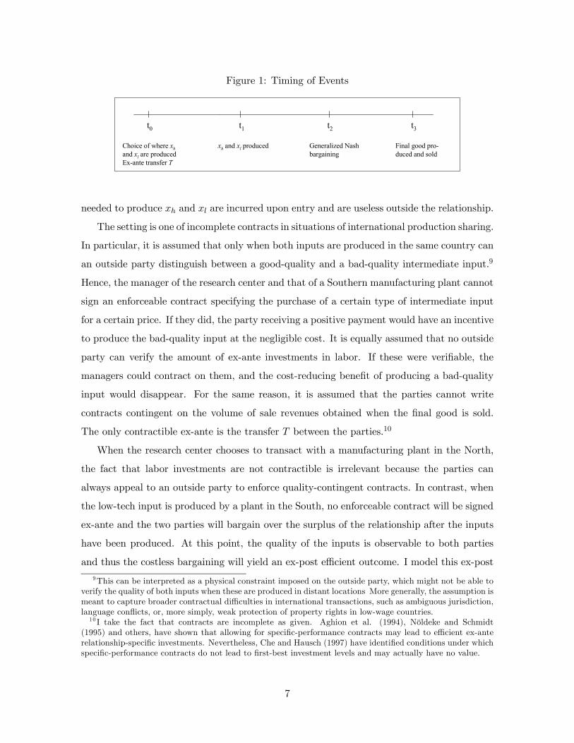
Figure 1: Timing of Events

t0

Choice of where xhand xl are producedEx-ante transfer T

t2

Generalized Nash bargaining

t3

Final good pro-duced and sold

t1

xh and xl produced

needed to produce xh and xl are incurred upon entry and are useless outside the relationship.

The setting is one of incomplete contracts in situations of international production sharing.

In particular, it is assumed that only when both inputs are produced in the same country can

an outside party distinguish between a good-quality and a bad-quality intermediate input.9

Hence, the manager of the research center and that of a Southern manufacturing plant cannot

sign an enforceable contract specifying the purchase of a certain type of intermediate input

for a certain price. If they did, the party receiving a positive payment would have an incentive

to produce the bad-quality input at the negligible cost. It is equally assumed that no outside

party can verify the amount of ex-ante investments in labor. If these were verifiable, the

managers could contract on them, and the cost-reducing benefit of producing a bad-quality

input would disappear. For the same reason, it is assumed that the parties cannot write

contracts contingent on the volume of sale revenues obtained when the final good is sold.

The only contractible ex-ante is the transfer T between the parties.10

When the research center chooses to transact with a manufacturing plant in the North,

the fact that labor investments are not contractible is irrelevant because the parties can

always appeal to an outside party to enforce quality-contingent contracts. In contrast, when

the low-tech input is produced by a plant in the South, no enforceable contract will be signed

ex-ante and the two parties will bargain over the surplus of the relationship after the inputs

have been produced. At this point, the quality of the inputs is observable to both parties

and thus the costless bargaining will yield an ex-post efficient outcome. I model this ex-post

9This can be interpreted as a physical constraint imposed on the outside party, which might not be able toverify the quality of both inputs when these are produced in distant locations More generally, the assumption ismeant to capture broader contractual difficulties in international transactions, such as ambiguous jurisdiction,language conflicts, or, more simply, weak protection of property rights in low-wage countries.10 I take the fact that contracts are incomplete as given. Aghion et al. (1994), Nöldeke and Schmidt

(1995) and others, have shown that allowing for specific-performance contracts may lead to efficient ex-anterelationship-specific investments. Nevertheless, Che and Hausch (1997) have identified conditions under whichspecific-performance contracts do not lead to first-best investment levels and may actually have no value.

7

bargaining as a Symmetric Nash Bargaining game in which the parties share equally the

ex-post gains from trade.11 Because the inputs are tailored specifically to the other party in

the transaction, if the two parties fail to agree on a division of the surplus, both are left with

nothing.

This completes the description of the model. The timing of events is summarized in

Figure 1.

2.2 Firm Behavior

As discussed above, the North has a sufficiently high productivity advantage in producing

the hi-tech input to ensure that xh is produced there. The decision of where to produce

the low-tech input is instead nontrivial. In his choice, the manager of the research center

compares the ex-ante profits associated with two options, which I analyze in turn.

A. Manufacturing by an Independent Plant in the North

Consider first the case of a research center that decides to deal with an independent man-

ufacturing plant in the North. In that case, the two parties can write an ex-ante quality-

contingent contract that will not be renegotiated ex-post. The initial contract stipulates

production of good-quality inputs in an amount that maximizes the research center’s ex-ante

profits, which from equations (1) and (2), and taking account of the transfer T , are given by

πN = λ1−αζαz xα(1−z)h xαzl − wNxh − wNxl. It is straightforward to check that this program

yields the following optimal price for the final good:

pN (z) =wN

α.

Because the research center faces a constant elasticity of demand, the optimal price is equal

to a constant mark-up over marginal cost. Ex-ante profits for the research center are in turn

equal to

πN (z) = (1− α)λ

µwN

α

¶−α/(1−α). (3)

B. Manufacturing by an Independent Plant in the South

Consider next the problem faced by a research center that decides to transact with a plant

in the South. As discussed above, in this case the initial contract only stipulates the transfer

T . The game played by the manager of the research center and that of the manufacturing

11 In Antràs (2003b), I extend the analysis to the case of Generalized Nash Bargaining.

8

plant is solved by backwards induction. If both producers make good-quality intermediate

inputs and the firms agree in the bargaining, the potential revenues from the sale of the final

good are R = λ1−αζαz xα(1−z)h xαzl . In contrast, if the parties fail to agree in the bargaining,

both are left with nothing. The quasi-rents of the relationship are therefore equal to sale

revenues, i.e., R. The Nash bargaining leaves each manager with one-half of these quasi-rents.

Rolling back in time, the research center manager sets xh to maximize 12R−wNxh, while the

manufacturing plant simultaneously chooses xl to maximize 12R − wSxl.12 Combining the

first-order conditions of these two programs yields the following optimal price for the final

good:

pS (z) =2¡wN¢1−z ¡

wS¢z

α.

If parties could write complete contracts in international transactions, the research center

would instead set a price equal to¡wN¢1−z ¡

wS¢z/α. The overinflated price reflects the

distortions arising from incomplete contracting. Intuitively, because in the ex-post bargaining

the parties fail to capture the full marginal return to their investments, they will tend to

underinvest in xh and xl. As a result, output will tend to be suboptimal and the move along

the demand function will also be reflected in an inefficiently high price.

Setting T so as to make the manufacturing plant break even leads to the following ex-

pression for the research center’s ex-ante profits:

πS (z) =

µ1− 1

2α

¶λ

Ã2¡wN¢1−z ¡

wS¢z

α

!−α/(1−α). (4)

2.3 The Equilibrium Choice

From comparison of equations (3) and (4), it follows that the low-tech input will be produced

in the South only if A (z) ≤ ω ≡ wN/wS , where

A(z) ≡Ã

1− α¡1− 1

2α¢ ¡

12

¢α/(1−α)!(1−α)/αz

. (5)

It is straightforward to show that A(z) is non-increasing in z for z ∈ [0, 1], with limz→0A(z) =

+∞ and A (1) > 1.13 This implies that (i) for high enough product-development intensities of

the final good, manufacturing is necessarily assigned to a manufacturing plant in the North;

and (ii) unless the wage in the North is higher than that in the South, manufacturing by an

12 It is easily checked that in equilibrium both parties receive a strictly positive ex-post payoff from producinga good-quality input. It follows that bad-quality inputs are never produced.13This follows from the fact that (1− αx)xα/(1−α) is increasing in x for α ∈ (0, 1) and x ∈ (0, 1).

9

Figure 2: The Choice of Location

z10 z

A(z)

ω

xl produced in the North xl produced in the South

independent plant in the South will never be chosen. Intuitively, the benefits of Southern

assembly are able to offset the distortions created by incomplete contracting only when the

manufacturing stage is sufficiently important in production or when the wage in the South is

sufficiently lower than that in the North. To make matters interesting, I assume that:

Condition 1: There exists a zc ∈ (0, 1) such that A (zc) < ω.14

This ensures that πN (zc) < πS (zc) for some zc ∈ (0, 1). Figure 2 depicts the profit-

maximizing choice of location as a function of z. It is apparent that:

Lemma 1 Under Condition 1, there exists a unique threshold z ∈ (0, 1) such that the low-

tech input is produced in the North if z < z ≡ A−1(ω), while it is produced in the South if

z > z ≡ A−1(ω), where A(z) is given by equation (5) and ω is the relative wage in the North.

From direct inspection of Figure 2, it is clear that an increase in the relative wage in the

North reduces the threshold z. Intuitively, an increase in ω makes Southern manufacturing

relatively more profitable and leads to a reduction in the measure of product-development

intensities for which the whole production process stays in the North.

14This condition will in fact be shown to necessarily hold in the general-equilibrium model (which is whyI avoid labelling it as an assumption), where the relative wage in the North will necessarily adjust to ensurepositive labor demand in the South.

10

2.4 Dynamics: The Product Cycle

As discussed in the introduction, one of the premises of Vernon’s (1966) original product-cycle

hypothesis is that as a good matures throughout its life cycle, it becomes more and more

standardized.15 Vernon believed that the unstandardized nature of new goods was crucial

for understanding that they would be first produced in a high-wage country.

To capture this standardization process in a simple way, consider the following simple

dynamic extension of the static model developed above. Time is continuous, indexed by t,

with t ∈ [0,∞). Consumers are infinitely lived and, at any t ∈ [0,∞), their preferences for

good y are captured by the demand function (1). The relative wage ω is assumed to be

time-invariant.16 The output elasticity of the low-tech input is instead assumed to increase

through time. In particular, this elasticity is given by

z(t) = h (t) , with h0(t) > 0, h (0) = 0, and limt→∞

h(t) = 1.

I therefore assume that the product-development intensity of the good is inversely related to

its maturity. Following the discussion in the introduction, this is meant to capture the idea

that most goods require a lot of R&D and product development in the early stages of their

life cycle, while the mere assembling or manufacturing becomes a much more significant input

in production as the good matures. I will take these dynamics as given, but it can be shown

that, under Condition 1, profits for the Northern research center are weakly increasing in z.

It follows that the smooth process of standardization specified here could, in principle, be

derived endogenously in a richer framework that incorporated some costs of standardization.17

Finally, I assume that the structure of firms is such that when Southern assembly is chosen,

the game played by the two managers can be treated as a static one and we can abstract from

an analysis of reputational equilibria. This is a warranted assumption when the separation

rate for managers is high enough or when future profit streams are sufficiently discounted.

With this simplified, dynamic set-up, the cut-off level z ≡ A−1(ω) is time-invariant, and

the following result is a straightforward implication of Lemma 1:

15 In discussing previous empirical studies on the location of industry, Vernon wrote: “in the early stagesof introduction of a new good, producers were usually confronted with a number of critical, albeit transitory,conditions. For one thing, the product itself may be quite unstandardized for a time; its inputs, its processing,and its final specifications may cover a wide range. Contrast the great variety of automobiles produced andmarketed before 1910 with the thoroughly standardized product of the 1930s, or the variegated radio designsof the 1920s with the uniform models of the 1930s.” (Vernon, 1966, p.197).16The latter assumption will be relaxed in the section 5, where ω will be endogenized.17For instance, if such costs were increasing in dz/dt, then a discrete increase in z would be infinitely costly.

A full fledged modeling of the standardization decision is left for future research.

11

Proposition 1 The model displays a product cycle. When the good is relatively new or

unstandardized, i.e., t ≤ h−1 (z), the manufacturing stage of production takes place in the

North. When the good is relatively mature or standardized, i.e., t > h−1 (z), manufacturing

is undertaken in the South.

Consider, for instance, the following specification of the standardization process:

z(t) = h (t) = 1− e−t/θ,

where 1/θ measures the rate at which 1− z falls towards zero, i.e., the rate of standardiza-

tion. With this functional form, the whole production process remains in the North until

the product reaches an age equal to θ ln³

11−z

´, at which point manufacturing is shifted to

the South. Naturally, production of the low-tech input is transferred to the South earlier,

the higher is the speed of standardization, 1/θ, and the lower is the threshold intensity z.

Furthermore, because the cut-off z is itself a decreasing function of ω, it follows that the

higher is the relative wage in the North, the earlier will production transfer occur.18

As argued in the introduction, the fact that international contracts are not perfectly en-

forceable is important for product cycles to emerge. To illustrate this, consider the case in

which the quality of intermediate inputs were verifiable by an outside court even in interna-

tional transactions, so that the manager of the research center and that of the Southern man-

ufacturing plant could also write enforceable contracts. It is straightforward to check that, in

such case, profits for the research center would be πS(z) = (1− α)λ³¡wN¢1−z ¡

wS¢z/α´−α/(1−α)

.

Comparing this expression with equation (3), it follows that labor demand in the South would

be positive if and only if ω ≥ 1 (this is the analog of Condition 1 above). If ω > 1, prof-

its would satisfy πN (z) ≤ πS(z) for all z ∈ [0, 1], with strict inequality for z > 0. The

production process would therefore be broken up from time 0 and no product cycles would

arise. If instead ω = 1, πN(z) and πS(z) would be identical for all z ∈ [0, 1] and the location

of manufacturing would be indeterminate, in which case product cycles would emerge with

probability zero.

Arguably, incomplete contracting is just one of several potential frictions that would make

manufacturing stay in the North for a period of time. It is important to emphasize, however,18Vernon (1966) hypothesized instead that before being transferred to low-wage countries, production would

first be located in middle-income countries for a period of time. An important point to notice is that in doingthe comparative statics with respect to ω, I have held the contracting environment constant. Recent empiricalstudies suggest that countries with better legal systems tend to have higher levels of per-capita income (Halland Jones, 1999, Acemoglu et al., 2001). If I allowed for this type of correlation in the model, productionmight not be transferred earlier, the higher ω.

12

that not any type of friction would give rise to product cycles in the model. The fact that

incomplete contracts distort both the manufacturing stage and the product development

stage in production is of crucial importance. For instance, introducing a transport cost or

a communication cost that created inefficiencies only in the provision of the low-tech input

would not suffice to give rise to product cycles in the model. In this paper, I choose to

emphasize the role of incomplete contracts because they are an important source of frictions

in the real world and, also, because they are a very useful theoretical tool for understanding

firm boundaries, which are the focus of the next section. The type of organizational cycles

unveiled by the empirical literature on the product cycle could not easily be rationalized

in theoretical frameworks in which production transfer to low-wage countries was delayed

merely by transport costs or communication costs.19 Instead, they will emerge naturally in

the extension below.

3 Firm Boundaries and the Product Cycle

Consider next the same set-up as in the previous section with the following new feature. The

research center is now given the option of vertically integrating the manufacturing plant and,

in the case of Southern assembly, becoming a multinational firm. Following the property-

rights approach of the theory of firm, vertical integration has the benefit of strengthening

the ex-post bargaining power of the integrating party (the research center), but the cost of

reducing the ex-post bargaining power of the integrated party (the manufacturing plant). In

particular, by integrating the production of the low-tech input, the manager of the manufac-

turing plant becomes an employee of the research center manager. This implies that if the

manufacturing plant manager refuses to trade after the sunk costs have been incurred, the

research center manager now has the option of firing the overseas manager and seizing the

amount of xl produced. As in Grossman and Hart (1986), ownership is identified with the

residual rights of control over certain assets. In this case, the low-tech input plays the role

of this asset.20

If there were no costs associated with firing the manufacturing plant manager, there

19To illustrate this point, consider the case in which the Northern productivity advantage in product develop-ment is bounded and the production process cannot be fragmented across borders (e.g., because of prohibitivetransport costs or communication costs). Under these circumstances, the whole production process wouldshift from the North to the South at some point along the life-cycle of the good, but the model would deliverno predictions for the dynamic organizational structure of firms.20See Antràs (2003a) and Antràs and Helpman (2004) for related set-ups.

13

would be no surplus to bargain over after production, and the manufacturing plant manager

would ex-ante optimally set xl = 0 (which of course would imply y = 0). In that case,

integration would never be chosen. To make things more interesting, I assume that firing

the manufacturing plant manager results in a negative productivity shock that leads to a

loss of a fraction 1 − δ of final-good production. Under this assumption, the surplus of the

relationship remains positive even under integration.21 I take the fact that δ is strictly less

than one as given, but this assumption could be rationalized in a richer framework.

The rest of this section is structured as follows. I will first revisit the static, partial-

equilibrium model developed in section 2. Next, I will analyze the dynamics of the model

and discuss the implications of vertical integration for this new view of the product cycle.

3.1 Firm Behavior

In section 2.2, I computed ex-ante profits for the research center under two possible modes of

organization: (A) manufacturing by an independent plant in the North; and (B) manufactur-

ing by an independent plant in the South. The possibility of vertical integration introduces

two additional options: manufacturing by a vertically integrated plant in the North and man-

ufacturing by a vertically integrated plant in the South. Because contracts are assumed to

be perfectly enforceable in transactions involving two firms located in the same country, it is

straightforward to show that the first of these new options yields ex-ante profits identical to

those in case (A). As is well known from the property-rights literature, in a world of com-

plete contracts, ownership structure is both indeterminate and irrelevant. In contrast, when

Southern assembly is chosen, the assignment of residual rights is much more interesting.

C. Manufacturing by a Vertically-Integrated Plant in the South

Consider then the problem faced by a research center and its integrated manufacturing

plant in the South. If both managers decide to make good-quality intermediate inputs and

they agree in the bargaining, the potential revenues from the sale of the final good are

again R = λ1−αζαz xα(1−z)h xαzl . In contrast, if the parties fail to agree in the bargaining, the

product-development manager will fire the manufacturing plant manager, who will be left

with nothing. The research center will instead be able to sell an amount δy(i) of output,

which using equation (1) will translate into sale revenues of δαR. The quasi-rents of the

21The fact that the fraction of final-good production lost is independent of z simplifies the analysis but isnot necesary for the qualitative results discussed below.

14

relationship are therefore given by (1− δα)R. Symmetric Nash bargaining leaves each party

with its default option plus one-half of the quasi-rents. The research center therefore sets xh

to maximize 12 (1 + δα)R − wNxh, while the Southern manufacturing plant simultaneously

chooses xl to maximize 12 (1− δα)R − wSxl. Relative to case (B) in section 2, integration

enhances the research center’s incentives to invest (12 (1 + δα) > 12) but, at the same time, it

reduces the manufacturing plant’s incentives to invest. Combining the first-order conditions

of these two programs yields the following optimal price for the final good:

pSM (z) =2¡wN¢1−z ¡

wS¢z

α (1 + δα)1−z (1− δα)z.

Incomplete contracting again distorts the optimal price charged for the final good. Notice,

however, that in this case the distortions are higher, the higher is z. Setting T so as to

make the integrated manufacturing plant break even leads to the following expression for the

research center’s ex-ante profits:

πSM (z) =

µ1− 1

2α (1 + δα (1− 2z))

¶λ

Ã2¡wN¢1−z ¡

wS¢z

α (1 + δα)1−z (1− δα)z

!−α/(1−α), (6)

where the subscriptM reflects the fact that the research center becomes a multinational firm

under this arrangement.

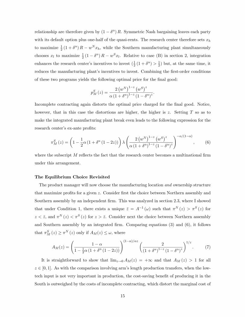
The Equilibrium Choice Revisited

The product manager will now choose the manufacturing location and ownership structure

that maximize profits for a given z. Consider first the choice between Northern assembly and

Southern assembly by an independent firm. This was analyzed in section 2.3, where I showed

that under Condition 1, there exists a unique z = A−1 (ω) such that πN (z) > πS (z) for

z < z, and πN (z) < πS (z) for z > z. Consider next the choice between Northern assembly

and Southern assembly by an integrated firm. Comparing equations (3) and (6), it follows

that πSM (z) ≥ πN (z) only if AM(z) ≤ ω, where

AM(z) =

Ã1− α

1− 12α (1 + δα (1− 2z))

!(1−α)/αz µ2

(1 + δα)1−z (1− δα)z

¶1/z. (7)

It is straightforward to show that limz→0AM(z) = +∞ and that AM (z) > 1 for all

z ∈ [0, 1]. As with the comparison involving arm’s length production transfers, when the low-

tech input is not very important in production, the cost-saving benefit of producing it in the

South is outweighed by the costs of incomplete contracting, which distort the marginal cost of

15

production of both the hi-tech and the low-tech inputs.22 It thus follows from this discussion

that, as in section 2, the low-tech input will again be produced in the North whenever z is

sufficiently low, that is, whenever the good is sufficiently unstandardized.

Consider next the choice between Southern assembly by an independent firm (or out-

sourcing) and Southern assembly by an integrated firm (or insourcing). It is straightforward

to check that insourcing will dominate outsourcing whenever AM(z) < A (z), while outsourc-

ing will dominate insourcing whenever AM(z) > A (z).23 Furthermore, the following result —

analogous to Proposition 1 in Antràs (2003a) — is proved in Appendix A.1.

Lemma 2 There exists a unique cutoff zMS ∈ (0, 1) such that AM(zMS) = A (zMS). Fur-

thermore, AM(z) < A (z) for 0 < z < zMS, and AM(z) > A (z) for zMS < z ≤ 1.

Proof. See Appendix A.1.

This implies that there exists a unique cutoff zMS such that insourcing dominates out-

sourcing for all z < zMS , with the converse being true for z > zMS . The logic of this result

lies at the heart of Grossman and Hart’s (1986) seminal contribution. When contracts gov-

erning transactions are incomplete, ex-ante efficiency dictates that residual rights should be

controlled by the party undertaking a relatively more important investment in a relation-

ship. If production of the final good requires mostly product development (i.e., z is low),

the investment made by the manufacturing plant manager will be relatively small, and thus

it will be optimal to assign the residual rights of control to the research center. Conversely,

when the low-tech input is important in production, the research center will optimally choose

to tilt the bargaining power in favor of the manufacturing plant by giving away these same

residual rights.

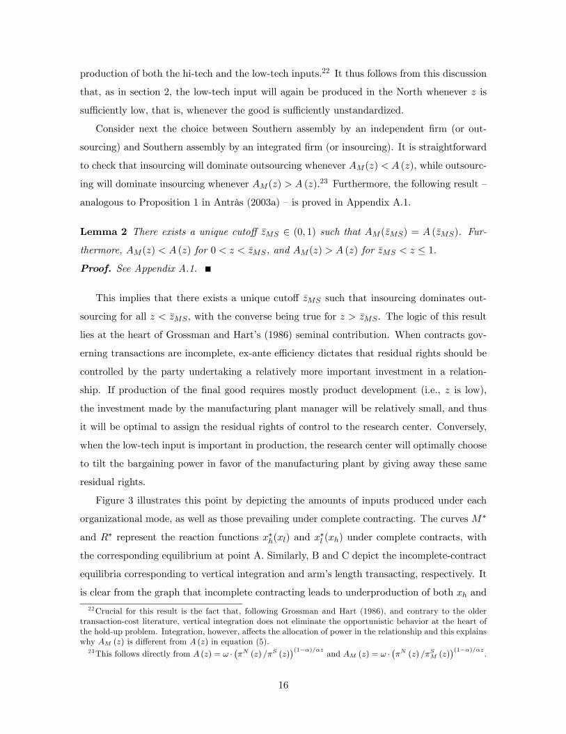
Figure 3 illustrates this point by depicting the amounts of inputs produced under each

organizational mode, as well as those prevailing under complete contracting. The curves M∗

and R∗ represent the reaction functions x∗h(xl) and x∗l (xh) under complete contracts, with

the corresponding equilibrium at point A. Similarly, B and C depict the incomplete-contract

equilibria corresponding to vertical integration and arm’s length transacting, respectively. It

is clear from the graph that incomplete contracting leads to underproduction of both xh and

22Crucial for this result is the fact that, following Grossman and Hart (1986), and contrary to the oldertransaction-cost literature, vertical integration does not eliminate the opportunistic behavior at the heart ofthe hold-up problem. Integration, however, affects the allocation of power in the relationship and this explainswhy AM (z) is different from A (z) in equation (5).23This follows directly from A (z) = ω · πN (z) /πS (z)

(1−α)/αzand AM (z) = ω · πN (z) /πSM (z)

(1−α)/αz.

16

Figure 3: Underproduction and Ownership Structure

xl

xh

RV

M *

xh*

xhV

xl*

R *

MV MO

RO

xlV xl

O

xhO

A

B

C

xl. The crucial point to notice from Figure 3, however, is that because the manufacturing

plant has relatively less bargaining power under integration, the underproduction in xl is

relatively higher under integration than under outsourcing. Furthermore, the more important

is the low-tech input in production, the more value-reducing will the underinvestment in xl

be. It thus follows that profits under integration relative to those under outsourcing will tend

to be lower, the more important is the low-tech input in production (i.e., the higher z).

A corollary of Lemmas 1 and 2 is that, as in section 2, when z is sufficiently high (i.e., when

z > max {z, zMS}), the low-tech input will again be produced in the South by a nonintegrated

manufacturing plant. Remember also that we have established that for sufficiently low z, the

low-tech input is necessarily produced in the North. It remains to analyze what happens for

intermediate values of z, where multinational firms may potentially arise.

Notice first that if AM (z) > ω for all z ∈ [0, 1], Northern assembly strictly dominates

Southern insourcing for all z ∈ [0, 1] and multinational firms do not emerge. Furthermore, in

such case, the choice between Northern assembly and foreign outsourcing is identical to that

in section 2.24 Let us therefore focus on the case in which AM (z) < ω for some z ∈ [0, 1].

This analysis is simplified by assuming that δ is not too high, which ensures that the function

AM(z) is a decreasing function of z for all z ∈ [0, 1].25 As shown in Appendix A.2, a sufficient24 In particular, because A (zMS) = AM (zMS) > ω and given that A0 (z) < 0, it must be the case that

z > zMS , and thus the equilibrium is as described in Lemma 1.25The AM (z) curve is decreasing in z for low values of z even when δ approaches one. Assumption 1 rules

out cases in which AM(z) might tilt up for high values of z. Such cases are discussed in Appendix A.2. The

17

Figure 4: Firm Boundaries and the Product Cycle

z10

ω

xl produced in North

xl produced in Southby unaffiliated plant

xl produced in Southby subsidiary

MSMN z z z

A(z)(z)AM

z10

ω

xl produced in the North xl produced in the South by unaffiliated plant

(z)AM

A(z)

z z z MNMS

(a) An equilibrium without multinationals (b) An equilibrium with multinationals

condition for this to be the case is:

Assumption 1: δα ≤ 1/2.

Under Assumption 1, there exists a unique cutoff zMN = A−1M (ω) ∈ (0, 1) such that

πN (z) > πSM (z) for z < zMN , and πN (z) < πSM (z) for z > zMN . This in turn implies that

the low-tech input will be produced in the North only if z < min {z, zMN}. Furthermore, it

is easily verified that the three thresholds z, zMN , and zMS must satisfy one of the following:

(i) zMS = z = zMN , (ii) zMS < z < zMN , or (iii) zMN < z < zMS .26

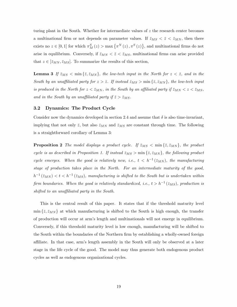
Figure 4 is instructive in understanding this result. The figure depicts the curves A(z)

and AM(z), which under Assumption 1, are both decreasing in z. Lemma 2 ensure that these

curves intersect just once and that A(z) > AM(z) if and only if z < zMS . For any relative

wage ω, it is clear that either zMS < z < zMN (left panel) or zMN < z < zMS (right panel).

The case zMS = z = zMN occurs with probability zero and will be ignored hereafter.

As indicated in both panels in Figure 4, for a low enough value for z, the benefits from

Southern assembly are too low relative to the distortions from incomplete contracting, and xl

is produced in the North. Furthermore, for a sufficiently high value of z, a profit-maximizing

research center will decide to outsource the manufacturing input to an independent manufac-

results are very similar with the exception that under certain parameter values, the model may feature morecomplex product-cycle dynamics.26To see this, notice for instance that zMS < z if and only if both A (zMS) > ω and Θ(z) < 1. But the

latter can only be true if A(z)/A(z) = ω/A(z) < 1, which implies z < zMN .

18

turing plant in the South. Whether for intermediate values of z the research center becomes

a multinational firm or not depends on parameter values. If zMS < z < zMN , then there

exists no z ∈ [0, 1] for which πSM (z) > max©πN (z) , πS (z)

ª, and multinational firms do not

arise in equilibrium. Conversely, if zMN < z < zMS , multinational firms can arise provided

that z ∈ [zMN , zMS]. To summarize the results of this section,

Lemma 3 If zMS < min {z, zMN}, the low-tech input in the North for z < z, and in the

South by an unaffiliated party for z > z. If instead zMS > min {z, zMN}, the low-tech input

is produced in the North for z < zMN , in the South by an affiliated party if zMN < z < zMS,

and in the South by an unaffiliated party if z > zMS.

3.2 Dynamics: The Product Cycle

Consider now the dynamics developed in section 2.4 and assume that δ is also time-invariant,

implying that not only z, but also zMN and zMS are constant through time. The following

is a straightforward corollary of Lemma 3:

Proposition 2 The model displays a product cycle. If zMS < min {z, zMN}, the product

cycle is as described in Proposition 1. If instead zMS > min {z, zMN}, the following product

cycle emerges. When the good is relatively new, i.e., t < h−1 (zMN ), the manufacturing

stage of production takes place in the North. For an intermediate maturity of the good,

h−1 (zMN) < t < h−1 (zMS), manufacturing is shifted to the South but is undertaken within

firm boundaries. When the good is relatively standardized, i.e., t > h−1 (zMS), production is

shifted to an unaffiliated party in the South.

This is the central result of this paper. It states that if the threshold maturity level

min {z, zMN} at which manufacturing is shifted to the South is high enough, the transfer

of production will occur at arm’s length and multinationals will not emerge in equilibrium.

Conversely, if this threshold maturity level is low enough, manufacturing will be shifted to

the South within the boundaries of the Northern firm by establishing a wholly-owned foreign

affiliate. In that case, arm’s length assembly in the South will only be observed at a later

stage in the life cycle of the good. The model may thus generate both endogenous product

cycles as well as endogenous organizational cycles.

19

4 Empirical Evidence

This section reviews some implications of this extended version of the model and contrasts

them with the findings of the empirical literature on the product cycle. For simplicity, I will

mostly focus on the case in which zMS > min {z, zMN}, so that the model features both

intrafirm as well as arm’s-length production transfers.

Consider first the time-series implications of the model. These are well summarized by

Proposition 2. The model predicts that industries will emerge in low-wage countries only

with some lag. Furthermore, the model predicts that in the initial phases of the presence of

the industry in the South, foreign direct investment from rich countries should constitute an

important part of the industry. Eventually, unaffiliated domestic producers should gain the

bulk of the Southern market share, but importantly the model predicts that foreign licensing

should still play an important role in those later phases.

The model is consistent with the evolution of the Korean electronics industry from the

early 1960s to the late 1980s.27 In the early 1960s, Korean electronic firms were producing

mostly low-quality consumer electronics for their domestic market. The industry took off in

the late 1960s with the establishment of a few large U.S. assembly plants, almost all wholly

owned, followed in the early 1970s by substantial Japanese investments.28 These foreign

subsidiaries tended to assemble components exclusively for export using imported parts. In

this initial phase, foreign affiliates were responsible for 71% of exports in electronics, with the

percentage reaching 97% for the case of exports of integrated circuits and transistors, and

100% for memory planes and magnetic heads. In the 1970s and 1980s domestic Korean firms

progressively gained a much larger market share, but the strengthening of domestic electronic

companies was accompanied by a considerable expansion of technology licensing from foreign

firms. Indeed, as late as 1988, 60% of Korean electronic exports were recorded as part of an

Original Equipment Manufacturing (OEM) transaction.29 The percentage approached 100%

in the case of exports of computer terminals and telecommunications equipment. Korean

giants such as Samsung or Goldstar were heavily dependent on foreign licenses and OEM

agreements even up to the late 1980s.30

27The following discussion is based on Bloom (1992), UNCTAD (1995, pp. 251-253), and Cyhn (2002).28Motorola established a production plant in Korea in 1968. Other U.S. based multinationals establishing

subsidiaries in Korea during this period include Signetics, Fairchild and Control Data.29OEM is a form of subcontracting which as Cyhn’s (2002) writes “occurs when a company arranges for an

item to be produced with its logo or brand name on it, even though that company is not the producer”.30As pointed out by a referee, a caveat in mapping Proposition 2 with the evolution of the Korean electronics

industry is that, during this period, Korean wages were growing faster than U.S. wages (i.e., ω was steadily

20

At a more micro level, several cross-sectional implications of the model are consistent with

the findings of the empirical literature on the product cycle. To see this, imagine attempting

to test the model with data on a cross-section of production transfers. The model would then

predict that the probability of a particular transfer occurring within firm boundaries should

be decreasing in the maturity of the product at the time of the transfer. This maturity should

in turn be negatively correlated with the age of the product and positively correlated with

both its R&D intensity as well as with its speed of standardization.

Mansfield and Romeo (1980) analyzed 65 technology transfers by 31 U.S.-based firms in

a variety of industries. They found that, on average, U.S.-based firms tended to transfer

technologies internally to their subsidiaries within 6 years of their introduction in the United

States. The average lag for technologies that were transferred through licensing or through

a joint venture was instead 13 years. Similarly, after surveying R&D executives of 30 U.S.

based multinational firms, Mansfield, Romeo, and Wagner (1979) concluded that for young

technologies (less than 5 years old), internal technology transfer tended to be preferred to

licensing, whereas for more mature technologies (between 5 and 10 years), licensing became

a much more attractive choice.31

In more detailed studies, Davidson and McFetridge (1984, 1985) looked at 1,376 internal

and arm’s-length transactions involving high-technology products carried out by 32 US.-based

multinational enterprises between 1945 and 1975. Their logit estimates indicated that the

probability of internalization was indeed higher the newer and more radical was a technology

and the larger was the fraction of the transferor’s resources devoted to scientific R&D.

There is also some evidence that the probability of internalization might be decreasing

in the speed of standardization. Using a sample of 350 US firms, Wilson (1977) indeed

concluded that licensing was more attractive the less complex was the good involved, with

his measure of complexity being positively correlated with the amount of R&D undertaken

for its production. In their study of the transfer of 35 Swedish innovations, Kogut and Zander

(1993) similarly found that the probability of internalization was lower the more codifiable

fall). Notice, however, that because zMS is independent of ω, the model would still predict the simple three-stage product cycle provided that ω does not fall at a rate faster than A (z) and AM (z), as would be the caseif the good standardizes at a sufficiently fast rate.31 In the previous case of the Korean electronics industry, there is also some evidence that “Northern” firms

did not license their leading edge technologies to their Korean licensees. For instance, in 1986, Hitachi licensedto Goldstar the technology to produce the 1-megabyte Dynamic Random Access Memory (DRAM) chip, whenat the same time it was shifting to the 4-megabyte DRAM chip. Similarly, Phillips licensed the productionof CD players to ten Korean producers, while keeping within firm boundaries the assembly of their deckmechanisms.

21

and teachable and the less complex was the technology.

The dataset used by Davidson and McFetridge (1985) also includes information on the

characteristics of the country receiving the transfer. The model predicts that an equilibrium

with multinational firms is more likely the higher is zMS relative to the other two thresholds

z and zMN . In section 2.3, I showed that z is a decreasing function of the relative wage ω. By

way of implicit differentiation, and making use of Assumption 1, one can show that zMN is

also decreasing in ω. The choice between an independent and an integrated Southern supplier,

as captured by the threshold zMS is instead unaffected by the relative wage in the North.32 It

thus follows that in a cross-section of production transfers, the probability of internalization

should be decreasing in the labor costs of the recipient country. This prediction is consistent

with the findings of Davidson and McFetridge (1985). In their sample of 1,376 transfers,

they found that a higher GNP per capita of the recipient country (arguably, a proxy for

ω in the model) was associated with a lower probability of internalization. Importantly,

their results are robust to controlling for several institutional characteristics of the recipient

country (remember the discussion in footnote 18).33

One further implication of the model is that relative to the case in which only arm’s length

transactions are permitted, the emergence of intrafirm production transfer by multinational

firms accelerates the shift of production towards the South (remember that zMN < z when-

ever multinational firms are active in the model). This result fits well Moran’s (2001) recent

study of the effects of domestic-content, joint-venture, and technology-sharing mandates on

production transfer to developing countries. Plants in host countries that impose such re-

strictions, he writes, “utilize older technology, and suffer lags in the introduction of newer

processes and products in comparison to wholly owned subsidiaries without such require-

ments” (p. 32). He also describes an interesting case study. In 1998, Eastman Kodak agreed

to set up joint ventures with three designated Chinese partners. These joint ventures special-

ized in producing conventional films under the Kodak name. When the Chinese government

allowed Kodak to establish a parallel wholly owned plant, Kodak shifted to this affiliate the

manufacturing of the latest digitalized film and camera products (p. 36).

32This follows directly from the assumption of Cobb-Douglas technology and isolates the partial-equilibriumdecision to integrate or outsource from any potential general-equilibrium feedbacks. This implied block-recursiveness is a useful property for solving the model sequentially, but the main results should be robust tomore general specifications of technology.33 In parallel work using aggregate industry data from the U.S. Department of Commerce, Contractor (1984)

found similar results.

22

5 Incomplete Contracts and the Product Cycle in GeneralEquilibrium

In this section, the partial-equilibrium model developed above is embedded in a general-

equilibrium framework with varieties in different sectors standardizing at different rates. I

will first solve for the time-path of the relative wage in the two countries and show that the

equilibrium wage in the North is necessarily higher than that in the South. Next, I will study

some macroeconomic and welfare implications of this new view of the product cycle.

5.1 Set-up

Consider again a world with two countries, the North and the South. The North is endowed

with LN units of labor at any time t ∈ (0,∞), while the Southern endowment is also constant

and equal to LS. At each period t, there is a measure N(t) of industries indexed by j, each

producing an endogenously determined measure nj(t) of differentiated goods. I consider an

economy in which exogenous inventions continuously increase the stock of existing industries.

In particular, I let N(t) = gN(t) and N (0) = N0 > 0. Hence, in any period t there are

N(t) = N0egt industries producing varieties of final goods. Preferences of the infinitely-lived

representative consumer in each country are given by:

U =

Z ∞

0e−ρt

Z N(t)

0log

ÃZ nj(t)

0yj (i, t)

α di

!1/αdjdt, (8)

where ρ is the rate at which the consumer discounts future utility streams. Notice that all

industries are viewed as symmetric with a unitary elasticity of substitution between them.

The varieties of differentiated goods also enter symmetrically into (8), but with an elasticity

of substitution equal to 1/(1 − α) > 1. Because the economy has no means of saving and

preferences are time-separable, the consumer maximizes utility period by period and the

discount rate plays no role in the model (other than to make the problem bounded).34 As is

well known, the instantaneous utility function in (8) gives rise to a constant price-elasticity

of demand for any variety i in any industry j:

yj (i, t) = λj(t)pj (i, t)−1/(1−α) , (9)

34For simplicity, equation (8) assumes an infinite intertemporal elasticity of substitution in aggregate con-sumption. Because of the static nature of the consumer’s problem, this is an immaterial assumption and thesame results would apply for any well-behaved instantaneous utility function.

23

where

λj(t) =1

N(t)

E (t)R nj(t)0 pj(i0, t)−α/(1−α)di0

, (10)

and E (t) is total world spending in period t. Because firms take λj(t) as given, each producer

of a final-good variety faces a demand function analogous to that in equation (1) in the

partial-equilibrium model above.

Production of each final-good variety is also as described in sections 2 and 3, with the

additional assumption that, at every period t, production of each variety also requires a

fixed cost of f units of labor in the country where the hi-tech input is produced (i.e., the

North). It is assumed that all producers in a given industry share the same technology as

specified in (2), with a common time-varying elasticity z(t− t0j , θj), where t0j is the date at

which industry j is born and θj is an industry-specific parameter that captures differences

in the speed of standardization across industries in the same cohort. As before, I assume

that ∂z(·)/∂ (t− t0j) > 0, z(0, θj) = 0, and limt−t0j→∞ z(t − t0j , θj) = 1. That is, varieties

in a given industry j are produced for the first time at t0j using only the hi-tech input, and

then all standardize at a common rate. The industry-specific parameter θj is assumed to be

drawn at period t0j from a time-invariant distribution G (θ). To isolate the effect of cross-

industry differences in maturity and in standardization rates, I assume that the technology

for producing intermediate inputs, as well as fixed costs, are identical across industries and

varieties.

Firm structure is as described above, with the additional assumption that there is free

entry at every period t, so that the measure nj (t) of varieties in each industry always adjusts

so as to make all research centers break even. The lack of profits in equilibrium is implied by

the fact that technology is a function of the industry’s age and not of the age of the producer

of a particular variety. Furthermore, as in section 2.4, I assume that firm structure is such

that when Southern procurement is chosen, the game played by the two managers can be

treated as a static one and we can abstract from an analysis of reputational equilibria. The

contracting environment is also analogous to that of the partial-equilibrium model and, in

particular, the parameter δ is time-invariant and common for all varieties and industries.

These assumptions, coupled with the absence of means of saving in the model, permit a

period-by-period analysis of the dynamic, general-equilibrium model.

24

5.2 General Equilibrium without Multinational Firms

To better illustrate the workings of the general equilibrium, it is useful to first study the

case in which intrafirm production transfers are ruled out. Consider then the equilibrium

in any industry j at any period t ∈ [0,∞).35 Facing the same technology and contracting

environment, all producers in the same industry will necessarily set the same price and

therefore will earn the same profits. It follows that letting again z (t) ≡ A−1(ω (t)), the

low-tech input will be produced in the North if z(t − t0j , θj) < z (t), and in the South if

z(t − t0j , θj) > z (t), with the choice remaining indeterminate for z(t − t0j , θj) = z (t). The

equilibrium number of varieties produced in industry j at time t can be solved for by using

prices to compute λj(t), and then setting operating profits in (3) and (4) equal to fixed costs,

as dictated by free entry. This yields

nj(t) =

⎧⎨⎩ (1− α)E(t)/£N(t)wN(t)f

¤if z(t− t0j , θj) < z (t)¡

1− 12α¢E(t)/

£N(t)wN (t)f

¤if z(t− t0j , θj) > z (t)

. (11)

Naturally, the equilibrium number of varieties in industry j depends positively on total spend-

ing in the industry and negatively on fixed costs.

Free entry ensures that profits are zero and thus all income accrues to labor. In the

general equilibrium, world income equals world spending on all goods:

wN(t)LN + wS(t)LS = E(t), (12)

and the labor market clears in each country. By Walras’ law, we can focus on the equi-

librium in the labor market in the South. Southern labor will only be demanded by those

manufacturing plants belonging to an industry with z(t − t0j , θj) > z (t). It is straightfor-

ward to show that labor demand by each manufacturing plant in the South can be expressed

as LSl =

12αz (·)E(t)/

¡wS (t)N(t)nj (t)

¢. Denoting by Ft(z) the fraction of industries with

z(t− t0j , θj) < z (t) at time t and letting ft(z) be the associated probability density function,

the Southern labor-market clearing condition can be expressed as:Z 1

z(t)

1

2αzE(t)ft(z)dz = wS(t)LS . (13)

Defining ξt (a, b) ≡R ba zft(z)dz and using (12), equation (13) can be rewritten as follows:

ω (t) = Bt(z (t)) ≡2− αξt (z (t) , 1)

αξt (z (t) , 1)

LS

LN. (14)

35The unit elasticity of substitution between varieties in different industries implies that we can analyzefirm behavior in each industry independently. This assumption, which is made for tractability, comes at thecost of obscuring potentially interesting cross-industry interactions in the production transfer decision.

25

Figure 5: General Equilibrium

z10

ω

ω

A(z)B(z)

z

Bt(z (t)) is an increasing function of z (t) satisfying Bt(0) > 0 and limz(t)→1Bt(z (t)) = +∞.

Intuitively, the higher is z (t), the lower is labor demand in the South for a given ω (t), so an

increase in ω (t) is necessary to bring the Southern labor market back to equilibrium. When

z (t) goes to 1, labor demand in the South goes to 0, and the required relative wage goes to

+∞.36 Figure 5 depicts the curve Bt(·) in the (z, ω) space.

The other equilibrium condition that pins down z (t) and ω (t) comes from the partial

equilibrium in section 2. In particular, since α is common across industries, z (t) is also

common across industries and is implicitly defined by the equal profitability condition ω (t) =

A(z (t)), where A(·) is defined in equation (5). Remember that A(z (t)) is a decreasing

function of z satisfying limz(t)→0A(z (t)) = +∞ and A(1) > 1. The function A(·) is depicted

in Figure 5 together with the function Bt(·). It is apparent from Figure 5 that there exists

a unique equilibrium pair (z (t) , ω (t)) at each period t ∈ [0,∞). Furthermore, the fact that

A(1) is greater than 1 ensures that the equilibrium wage in the North is higher than that in

the South, i.e., ω (t) > A (1) > 1. This implies that Condition 1 in section 2 necessarily holds

in the general equilibrium, thus granting validity to the analysis in sections 2 and 3.

It is interesting to notice that in spite of the heterogeneity in industry product-cycle

dynamics, the cross-sectional picture that emerges from the model is very similar to that in

the classical Ricardian model with a continuum of goods of Dornbusch et al. (1977). Notice,

36Since the North always produces the hi-tech input, labor demand in the North is positive even when z (t)goes to 0, and consequently Bt(0) is greater than zero.

26

however, that comparative advantage as represented by the curve A (·) is here endogenous and

arises from a combination of the Northern productivity advantage in product development,

the continuous standardization of goods, and the fact that contracts are incomplete.

The general equilibrium of the dynamic model is simply the sequence of period-by-period

general equilibria. Moreover, as shown on Appendix A.3, the economy will converge to a

stationary equilibrium in which the distribution function Ft(z) is time-invariant distribution,

and therefore z (t) and ω (t) are also time-invariant. In the equilibrium, all industries will

necessarily follow product cycles, with varieties being manufactured first in the North and

later in the South. In sum,

Proposition 3 The economy converges to a stationary equilibrium in which the relative wage

in the North is higher than one (ω > 1).

Proof. See Appendix A.3.

To illustrate the properties of the general equilibrium, consider again the particular func-

tional form:

z(t− t0j , θj) = 1− e−(t−t0j)/θj , (15)

so that the elasticity of output with respect to xh falls at a constant rate 1/θj . As before,

I will refer to 1/θj as industry j’s specific rate of standardization. From the discussion in

section 2.4, and given that the threshold z (t) is common across all industries, the model

predicts that industries with higher rates of standardization will transfer manufacturing to

the South earlier. Furthermore, in the general equilibrium, the cross-industry distribution

of standardization rates will have an additional effect on the timing of production transfer,

through its impact on the world distribution of product-development intensities, as given by

Ft(z). To see this, assume that θj is drawn at t0j from an exponential distribution with

mean θµ, i.e., G (θj) = 1−e−θj/θµ . Under these assumptions, Appendix A.3 shows that Ft(z)

converges to a time-invariant distribution function characterized by:

F (z) =gθµ ln

³11−z

´1 + gθµ ln

³11−z

´ . (16)

Furthermore, it is easily verified that the steady-state relative wage in the North is increasing

in the relative population size of the South LS/LN (as in Dornbusch et al., 1977) and in the

rate of exogenous invention g, while it is decreasing in the average rate of standardization

27

1/θµ (see Appendix A.3 for details). These comparative statics on the relative wage are

similar to those obtained by Krugman (1979) in the first paper to explore the macroeconomic

implications of the product cycle hypothesis.37 By endogenizing the timing of production

transfer, the present model delivers additional implications of a shift in the parameters g, θµ,

and LS/LN . For instance, an increase in the rate of invention g also leads to a reduction in

the time it takes for manufacturing of a particular good to be shifted to the South, which in

Krugman’s (1979) model depends only on the exogenous rate of imitation.38

In the working paper version of this paper (Antràs, 2003b), I also analyze the implica-

tions of a shift from the stationary equilibrium with incomplete contracts described above

to a stationary equilibrium with complete contracts. This improvement in the contracting

environment in international transactions is shown to unambiguously decrease the relative

wage in the North. Intuitively, Northern wages include a premium or rent that partly stems

from the incompleteness of international contracts. In a world of complete contracts, this

rent disappears and the relative wage in the North is reduced. In Antràs (2003b), I also show

that this shift towards complete contracts unambiguously increases the steady-state welfare

in the South, while having an ambiguous effect on steady-state Northern welfare.

5.3 General Equilibrium with Multinationals

Consider now the general equilibrium with multinational firms. In order to solve for the

equilibrium relative wage, it is useful to define ez(t) = min {zMN(t), z(t)} which, according to

Lemma 3 constitutes the threshold z above which production is shifted to the South. This is

the only variable apart from ω (t) that we need to pin down in the general equilibrium, given

that zMS does not depend on ω (t).

Computing labor demand by Southern manufacturing plants and imposing labor market

clearing in the South yields the following equilibrium condition relating ω and ez, which isanalogous to equation (14) (see Antràs, 2003b, for details):

ω = BMNE(ez) ≡⎧⎪⎨⎪⎩

2−α(1−δα)ξ(z,zMS)−αξ(zMS ,1)α(1−δα)ξ(z,zMS)+αξ(zMS ,1)

LS

LNif ez < zMS

2−αξ(z,1)αξ(z,1)

LS

LNif ez > zMS

. (17)

To save on notation, equation (17) already imposes that the distribution function Ft(z) will

converge to a time-invariant distribution, so that we can focus on the stationary general37Krugman (1979) concluded from his comparative static results that increased technological change in the

North redistributes income from the South to the North. My analysis suggests that this is not necessarily thecase when increased technological change takes the form of an increase in the rate at which goods standardize.38 Increases in θµ and LS/LN have an analogous effect on the timing of production transfer.

28

equilibrium and safely drop time subscripts. It is apparent from equation (17) that if ez >

zMS , the equilibrium is one without multinationals and the equilibrium condition naturally

collapses back to the one in the previous section, i.e., BMNE(ez) = B(ez). If instead ez <

zMS , multinationals indeed arise in equilibrium. Furthermore, from the standard logic in

Grossman and Hart (1986), an integrated manufacturing plant manager will underinvest

relatively more than a non-integrated one. Hence, for a given z, Southern labor demand

is relatively lower for vertically-integrated manufacturing plants, implying that BMNE(ez) >B(ez) for ez < zMS. Finally, notice that BMNE(ez) is a continuous and increasing function ofez, satisfying BMNE(0) > B(0) > 0 and limz→1BMNE(ez) = +∞.

As in section 5, the other equilibrium condition that pins down ez and ω comes from firm

behavior. In particular, because z is implicitly defined by ω = A(z), and zMN is implicitly

defined by ω = AM(zMN), it follows that ez = min {zMN , z} is implicitly defined by:

ω = AMNE(ez) ≡⎧⎨⎩ AM(ez) if ez < zMS

A(ez) if ez > zMS

. (18)

Again, if ez > zMS , multinationals are not active in equilibrium and AMNE(ez) = A(ez).On the other hand, as discussed in section 3, if ez < zMS, then it must be the case that

AMNE(ez) = AM(ez) < A(ez). Overall, AMNE(ez) is a continuous and (under Assumption 1)decreasing function of ez in [0, 1], satisfying limz→0AMNE(ez) = +∞ and AMNE(1) > 1.

It thus follows that there again exists a unique general-equilibrium (ez, ω) pair. Dependingon parameter values, the equilibrium is one without multinational firms (if the equilibriumez is lower than zMS) or one with multinational firms. In either case, industries necessarily

follow product cycles, with varieties in those industries first being manufactured in the North

and later in the South. In addition to these endogenous product cycles, an equilibrium with

multinational firms also features endogenous organizational cycles, with production being

shifted to the South first within firm boundaries and only later to independent Southern

firms.

Furthermore, given that AMNE(ez) ≤ A(ez) and BMNE(ez) ≥ A(ez) for all ez, it followsthat relative to a world with only arm’s length transacting, allowing for intrafirm production

transfer by multinational firms weakly accelerates the transfer of production to the South

(lowers ez), while having an ambiguous effect on the relative wage ω. This result complementsthe previous discussion on the effects of more liberal FDI policies on firm behavior, but it

29

illustrates how these policies may also produce significant general equilibrium effects.39

Finally, let us briefly return to the particular example analyzed above in which Ft (z)

converges to equation (16). As in the equilibrium with only arm’s length transacting, an

increase in g, θµ or LS/LN can be shown to increase the relative wage in the North and

to reduce the timing of production transfer ez. Furthermore, these parameter changes canbe shown to (weakly) increase the measure of product-development intensities for which

multinational firms exist. Intuitively, by creating an excess supply of Northern labor, an

increase in g, θµ, and LS/LN , raise both the relative wage as well as the threshold product-

development intensity (1− ez) below which manufacturing is transferred to the South. Fromthe result in Lemma 2, it then becomes more likely that the Northern research center will

decide to keep this transfer within firm boundaries.

6 Conclusions

This paper has presented a dynamic, general-equilibrium model featuring both endogenous

product cycles and endogenous organizational cycles. It has been argued that the same forces

that make firms choose to manufacture their new goods in high-wage countries can explain

why, when they decide to transfer production to low-wage countries, they might choose to do

so inside their firm boundaries. The model also delivers a few macroeconomic implications

that complement the work of Dornbusch et al. (1977) and Krugman (1979).

In contrast to previous general-equilibrium theories of the multinational firm, firm bound-

aries were not drawn appealing to technological considerations, such as economies of scale or

transport costs.40 As in Antràs (2003a), I instead set forth a purely organizational, property-

rights model of the multinational firm.41 Multinational firms emerged in equilibrium when-

ever transaction-cost minimization dictated that certain goods would be transacted more

39 In Antràs (2003b), I also analyze the welfare implications of a shift from a stationary equilibrium withonly arm’s-length transacting to a stationary equilibrium with multinational firms. It is shown that, providedthat its effect on relative wages is small enough, the steady-state welfare of both countries is higher in a worldwith intrafirm production transfers by multinational firms.40This previous literature builds on the seminal work of Helpman (1984) and Markusen (1984), and is

extensively reviewed in Caves (1996) and Markusen (1995). Ethier (1986), Ethier and Markusen (1996), andGlass and Saggi (2002) study the choice between foreign direct investment and licensing, but in frameworksin which the internalization decision is unrelated to the allocation of some residual rights of control.41This paper is related to an emerging literature on general-equilibrium models of ownership structure

(c.f., McLaren, 2000, Grossman and Helpman, 2002, Antràs, 2003a, Antràs and Helpman, 2004). In Antràs(2003a), I unveiled two systematic patterns in the volume of intrafirm trade, which I then rationalized in atheoretical framework that combined a Grossman-Hart-Moore view of the firm with a Helpman-Krugman viewof international trade. The model was extended in Antràs and Helpman (2004) to account for intraindustryheterogeneity in organizational choices.

30

efficiently within firm boundaries than at arm’s length. Relative to a world with only arm’s

length transacting, I showed that foreign direct investment might help alleviate contractual

frictions in global production sharing, thereby anticipating the transfer of certain stages of

the production to low-wage countries.

The simple model developed here has proven to be a useful lens through which to inter-

pret several findings in the international business literature. Nevertheless, much remains to

be done. For instance, the present framework has abstracted from at least one important

channel of production transfer, namely, imitation. Future efforts should also be directed

at incorporating elements of alternative theories of the firm to the study of international

patterns of specialization.

31

A Appendix

A.1 Proof of Lemma 2

Let Θ (z) = (AM (z)/A (z))z, which using equations (5) and (7) simplifies to

Θ (z) =

µ1− 1

2α

1− 12α (1 + δ (1− 2z))

¶(1−α)/αÃ1

(1 + δ)1−z

(1− δ)z

!.

Straightforward algebra delivers that Θ0 (z) > 0 if and only if

ln

µ1 + δα

1− δα

¶>

(1− α) δα

1− 12α (1 + δα (1− 2z))

.

The right hand side is decreasing in z and is therefore no larger than (1− α) δα/¡1− 1

2α (1 + δα)¢,

which in turn can be shown to be no larger than ln [(1 + δα) / (1− δα)]. To see this last statement,simply define the function ϑ (δ) = ln [(1 + δα) / (1− δα)]− (1− α) δα/

¡1− 1

2α (1 + δα)¢and notice it

is increasing in δ and satisfies ϑ (0) = 0.Next, the fact that (1− αx)xα/(1−α) is increasing in x for α ∈ (0, 1) and x ∈ (0, 1) implies that

Θ (0) < 1 and Θ (1) > 1. Hence, there exists a unique zMS such that Θ (z) < 1 for 0 < z < zMS ,Θ (z) > 1 for zMS < z < 1, and Θ (z) = 1 for z = zMS . Notice that Assumption 1 is not necessary forthis result. To complete the proof, note that for z ∈ (0, 1), AM (z) < A (z) if and only if Θ (z) < 1;AM (z) > A (z) if and only if Θ (z) > 1; and AM (z) = A (z) if and only if Θ (z) = 1. Finally, for z = 1,straightforward manipulation yields AM (1) > A (1).

A.2 Discussion of Assumption 1

As argued in the main text, the proof of Lemma 3 is straightforward when AM (z) is non-increasingin z for all z ∈ [0, 1]. Simple differentiation of equation (7) shows that this is the case whenever

r(z, δ, α) = ln

Ã1− 1

2α (1 + δα (1− 2z))1− α

µ1

2(1 + δα)

¶α/(1−α)!− δααz

1− 12α (1 + δα (1− 2z))

< 0.

It is easy to show that ∂r(·)/∂z ≥ 0 for all z ∈ [0, 1] (with strict inequality for z > 0), which impliesthat AM (z) will be decreasing for all z if the slope at z = 1 is negative. Differentiating r(1, δ, α) withrespect to δ, one can show that the slope at 1 is increasing in δ and is negative when evaluated atδ = (1/2)

1/α. It follows that if δα < 1/2, AM (z) is non-increasing in z for all z ∈ [0, 1].When δα > 1/2, the AM (z) curve will still be decreasing in z for sufficiently low z, but it may tilt

up when z is sufficiently close to one. In those cases, firm behavior will still be exactly as describedin Lemma 3 of section 4 provided that AM (z) equals ω for only one z ≤ z ≡ A−1 (ω). In other words,the AM (z) curve may intersect ω for high values of z, but this is immaterial because arm’s lengthtransacting dominates insourcing at those values of z.

Conversely, when δα > 1/2 and AM (z) equals ω for two values of z less than z, firm behavior is abit more complex than as described in Lemma 3.42 Denote these two thresholds by zMN and z0MN . Asin Lemma 3, firms will produce the low-tech input in the North for z < zMN , and they will contractwith an arm’s-length Southern producer when z > zMS . The only difference is that multinationalfirms will emerge only in the interval (zMN , z

0MN ) ⊂ (zMN , zMS), while Northern assembly will be

the preferred option not only for z < zMN but also for z ∈ (z0MN , zMS). In the dynamic extensionof the model, this implies that the model may predict that assembly returns to the North for someintermediate levels of standardization.

The economics behind these results are as follows. Incomplete contracting has two effects onprofits — compare equation (3) with equations (4) or (6). On the one hand, contractual frictions lead

42The convexity of AM (z) in [0, 1] ensures that AM (z) = ω for at most two values of z.

32

to underproduction of both xh and xl, which translates into lower sale revenues and profits. On theother hand, these frictions create rents, thereby increasing the fraction of revenues that producers areable to capture as operating profits. This second effect is second order in the sense that, holding relativewages constant, operating profits are always higher under complete contracts than under incompletecontracts. This is a desirable property of the model, because the existence of the second effect seemsmuch less robust to alternative modelling strategies.43 What matters for Lemma 3, however, is howthe overall distortions vary with z. This derivative tends to be dominated by the underproductioneffect which dictates that AM (z) be a non-increasing function of z for all z ∈ [0, 1]. For sufficientlyhigh δ, however, the second effect may actually dominate thus complicating the analysis.

A.3 Proof of Proposition 3

The fact that ω > 1 follows immediately from A (z) > 1 for all z ∈ [0, 1]. Furthermore, becauseAM (z) > 1 for all z ∈ [0, 1], this also holds in the general equilibrium with multinationals.

Let us now concentrate on the stationary properties of the model. Remember that it is sufficientto show that Ft (z) converges to a time invariant distribution. Assuming that the function z (·) isinvertible, the fraction of industries with z(t−t0j , θj) < z can be expressed as the following probability:

Ft (z) = Pr (z(t− t0j , θj) < z) = Pr (t− t0j < ψ (θj , z)) .

Using the fact that the number of industries grows at constant rate g, the distribution of t − t0jconditional on a particular realization of θj is simply

Ft (z|θj) = Pr (t− t0j < ψ (θj , z) |θj) =½1− e−g·ψ(θj ,z) if ψ (θj , z) ≤ tϕ0 (θj , z, t) if ψ (θj , z) > t

,

where ϕ0 (θj , z, t) depends on the characteristics of the initial N0 industries. As t → ∞, however,Ft (z|θj) converges to F (z|θj) = 1− e−g·ψ(θj ,z).

Next notice, that by the Glivenko-Cantelli theorem, the distribution of θj within each cohortconverges uniformly to G (θ). Because this distribution is time invariant, it follows that the overalldistribution for ψ (θj , z) ≤ t will also be characterized by G (θ). This in turn implies that as t→∞,the fraction of industries with z(t− t0j, θj) < z will converge to the time-invariant distribution:

F (z) =

Z ∞−∞

F (z|θj) dG (θj) .

Consider now the example in section 5 in which z(t − t0j , θj) = 1 − e−(t−t0j)/θj and G (θj) =1− e−θj/θµ . In this case, ψ (θj , z) = θj ln (1− z) and

F (z) =

Z ∞0

³1− (1− z)

gθj´· e−θj/θµ

θµ· dθj =

gθµ

³ln³

11−z

´´1 + gθµ

³ln³

11−z

´´as claimed in equation (16) above.

Letting f (z) be the corresponding probability density function and integrating by parts yields:

ξ (a, b) ≡Z b

a

zf(z)dz =a

1 + gθµ ln³

11−a

´ − b

1 + gθµ ln³

11−b

´ + Z b

a

1

1 + gθµ ln³

11−z

´dz (A.1)

To proof the claims in section 5.2 regarding the effects of g and θµ, we need only show that ∂ξ (z, 1) /∂g <0 and ∂ξ (z, 1) /∂θµ < 0. But this is follows from straightforward differentiation of ξ (z, 1) in (A.1).Similarly, to proof the claims in section 5.3, notice that ξ (ez, zMS)+ξ (zMS , 1) = ξ (ez, 1), and thereforeα (1− δα) ξ (ez, zMS) +αξ (zMS , 1) = α (1− δα) ξ (ez, 1) +αδαξ (zMS , 1). The results then follow againfrom ∂ξ (z, 1) /∂θµ < 0 and ∂ξ (z, 1) /∂g < 0.

43 In particular, by introducing a rent-absorbing fixed factor in production, this effect would disappear. Thisextension would, however, complicate the general equilibrium.

33

ReferencesAcemoglu, Daron, Simon Johnson, and James A. Robinson (2001), “The Colonial Origins of Com-

parative Development: An Empirical Investigation,” American Economic Review, 91, pp. 1369-1401.

Aghion, Philippe, Mathias Dewatripont and Patrick Rey (1994), “Renegotiation Design with Unver-ifiable Information,” Econometrica, 62:2, pp. 257-282.

Antràs, Pol (2003a), “Firms, Contracts, and Trade Structure,” Quarterly Journal of Economics,118:4, pp. 1375-1418.

Antràs, Pol (2003b), “Incomplete Contracts and the Product Cycle,” Working Paper no. 9945.Cambridge: Mass,: NBER.

Antràs, Pol and Elhanan Helpman (2004), “Global Sourcing,” Journal of Political Economy, 112:3,pp. 552-580.

Bloom, Martin (1992), Technological Change in the Korean Electronics Industry, Development CenterStudies, OECD, Paris.

Caves, Richard E. (1996), Multinational Enterprise and Economic Analysis, Second Edition, Cam-bridge University Press.

Che, Yeon-Koo and Donald B. Hausch (1999), “Cooperative Investments and the Value of Contract-ing,” American Economic Review, 89:1, pp. 125-147.

Contractor, Farok J. (1984), “Choosing between Direct Investment and Licensing: Theoretical Con-siderations and Empirical Tests,” Journal of International Business Studies, 15:3, pp. 167-188.

Cyhn, J. W. (2002), Technology Transfer and International Production: the Development of theElectronics Industry in Korea, Edward Elgar, Cheltenham.

Davidson, W. H. and Donald G. McFetridge (1984), “International Technology Transactions and theTheory of the Firm,” Journal of Industrial Economics, 32:3, pp. 253-264.

Davidson, W. H. and Donald G. McFetridge (1985), “Key Characteristics in the Choice of Interna-tional Technology Transfer Mode,” Journal of International Business Studies, 16:2, pp. 5-21.

Dornbusch, Rudiger, Stanley Fischer, and Paul A. Samuelson (1977), “Comparative Advantage,Trade and Payments in a Ricardian Model with a Continuum of Goods,” American EconomicReview, 67:5, pp. 823-839.

Ethier, Wilfred J. (1986), “The Multinational Firm,” Quarterly Journal of Economics, 101:4, pp.805-833.

Ethier, Wilfred J. and James R. Markusen (1996), “Multinational Firms, Technology Diffusion andTrade,” Journal of International Economics, 41:1, pp. 1-28.

Feenstra, Robert C. (1998), “Integration of Trade and Disintegration of Production in the GlobalEconomy,” Journal of Economic Perspectives, 12:4, 31-50.

Glass, Amy J., and Kamal Saggi (2002), “Licensing versus Direct Investment: Implications forEconomic Growth”, Journal of International Economics, 56:1, pp. 131-153.

Grossman, Sanford J., and Oliver D. Hart (1986), “The Costs and Benefits of Ownership: A Theoryof Vertical and Lateral Integration,” Journal of Political Economy, 94:4, pp. 691-719.

Grossman Gene M., and Elhanan Helpman (1991a), “Endogenous Product Cycles,” Economic Jour-nal, 101:4, pp. 1214-1229.

Grossman, Gene M., and Elhanan Helpman (1991b), “Quality Ladders and Product Cycles,” Quar-terly Journal of Economics, 106:2, pp. 557-586.

Grossman, Gene M., and Elhanan Helpman (2002), “Integration vs. Outsourcing in Industry Equi-librium,” Quarterly Journal of Economics, 117:1, pp. 85-120.

34

Gruber William, Dileep Mehta, and Raymond Vernon (1967), “The R & D Factor in InternationalTrade and International Investment of United States Industries,” Journal of Political Economy,75:1, pp. 20-37.

Hall, Robert E. and Charles I. Jones (1999), “Why Do Some Countries Produce So Much MoreOutput per Worker than Others?” Quarterly Journal of Economics, 114:1, pp. 83-116.

Hart, Oliver and John Moore (1990), “Property Rights and the Nature of the Firm,” Journal ofPolitical Economy, 98:6, pp. 1119-1158.

Helpman, Elhanan (1984), “A Simple Theory of International Trade with Multinational Corpora-tions”, Journal of Political Economy, 92:3, pp. 451-471.

Hirsch, Seev (1967), Location of Industry and International Competitiveness, Oxford: ClarendonPress.

Jensen, Richard and Marie Thursby (1987), “A Decision Theoretic Model of Innovation, TechnologyTransfer, and Trade,” Review of Economic Studies, 54:4, pp. 631-647.

Kogut, Bruce and Udo Zander (1993), “Knowledge of the Firm and the Evolutionary Theory of theMultinational Corporation,” Journal of International Business Studies, 24:4, pp. 625-645.

Krugman, Paul (1979), “A Model of Innovation, Technology Transfer, and the World Distributionof Income,” Journal of Political Economy, 87:2, pp. 253-266.

McLaren, John (2000), “Globalization and Vertical Structure,” American Economic Review, 90:5,pp. 1239-1254.

Mansfield, Edwin, and Anthony Romeo (1980), “Technology Transfer to Overseas Subsidiaries byU.S.-Based Firms,” Quarterly Journal of Economics, 95:4, pp. 737-750.

Mansfield, Edwin, Anthony Romeo, and Samuel Wagner (1979), “Foreign Trade and U. S. Researchand Development,” Review of Economics and Statistics, 61:1, pp. 49-57.

Markusen, James R. (1984), “Multinationals, Multi-Plant Economies, and the Gains from Trade”Journal of International Economics, 16, pp. 205-226.

Markusen, James R. (1995), “The Boundaries of Multinational Enterprises and the Theory of Inter-national Trade,” Journal of Economic Perspectives, 9:2, pp. 169-189.

Moran, Theodore H. (2001), Parental Supervision: The New Paradigm for Foreign Direct Investmentand Development, Washington DC: Institute for International Economics.

Nöldeke, Georg and Klaus M. Schmidt (1995), “Option Contracts and Renegotiation: A Solution tothe Hold-up Problem,” RAND Journal of Economics, 26:2, pp. 163-179.

Parry, Thomas G. (1975), “The Product Cycle and International Production: U.K. Pharmaceuti-cals,” Journal of Industrial Economics, 24:1, pp. 21-28.

Segerstrom, Paul S., T. C. A. Anant, and Elias Dinopoulos (1990), “A Schumpeterian Model of theProduct Life Cycle,” American Economic Review, 80:5, pp. 1077-1091.

UNCTAD (1995), World Investment Report: Transnational Corporations and Competitiveness, NewYork: United Nations.

Vernon, Raymond (1966), “International Investment and International Trade in the Product Cycle,”Quarterly Journal of Economics, 80:2, pp. 190-207.

Wells, Louis T. Jr. (1969), “Test of a Product Cycle Model of International Trade: U.S. Exports ofConsumer Durables,” Quarterly Journal of Economics, 83:1, pp. 152-162.

Williamson, Oliver E. (1985), The Economic Institutions of Capitalism, Free Press.

Wilson, Robert W. (1977), “The Effect of Technological Environment and Product Rivalry on R&DEffort and Licensing of Inventions,” Review of Economics and Statistics, 59:2, pp. 171-178.

Yi (2003), “Can Vertical Specialization Explain the Growth of World Trade?” Journal of PoliticalEconomy, 111:1, pp. 52-102.

35