Incorporating Exiting Vehicles in Capacity Estimation at Single-Lane U.S. Roundabouts Yuri Mereszczak Tel: (208) 885-9188, Fax: (208) 885-2877, [email protected]University of Idaho, National Institute for Advanced Transportation Technology 115 Engineering Physics Building, Moscow, ID 83844-0901, U.S.A. Michael Dixon, Ph.D. Tel: (208) 885-4338, Fax: (208) 885-2877 [email protected]University of Idaho, National Institute for Advanced Transportation Technology 115 Engineering Physics Building, Moscow, ID 83844-0901, U.S.A. Michael Kyte, Ph.D. Tel: (208) 885-6002, Fax: (208) 885-2877 [email protected]University of Idaho, National Institute for Advanced Transportation Technology 115 Engineering Physics Building, Moscow, ID 83844-0901, U.S.A. Lee Rodegerdts, P.E. Tel: (503) 535-7416, Fax: (503) 273-8169 [email protected]Kittelson and Associates, Inc. 610 SW Alder, Suite 700, Portland, OR 97205, U.S.A. Miranda Blogg, Ph.D., P.E. Tel: (954) 735-1245, Fax: (954) 735-9025 [email protected]Kittelson and Associates, Inc. 110 E. Broward Blvd., Suite 2410, Ft. Lauderdale, FL 33301, U.S.A. Submission Date: May 11, 2005 Word Count: 8597 Submitted for presentation at the Transportation Research Board National Roundabout Conference May 2005, Vail, Colorado
Transcript
Incorporating Exiting Vehicles in Capacity Estimation at Single-Lane U.S. Roundabouts
110 E. Broward Blvd., Suite 2410, Ft. Lauderdale, FL 33301, U.S.A.
Submission Date: May 11, 2005 Word Count: 8597
Submitted for presentation at the Transportation Research Board National Roundabout Conference May 2005, Vail, Colorado
Y. Mereszczak, M. Dixon, M. Kyte, L. Rodegerdts, M. Blogg 2
ABSTRACT
The current model used in the U.S. to predict approach capacity at a single-lane roundabout utilizes information about entry driver behavior in relation to the circulating stream of traffic only. No procedure is currently in place for incorporating exiting vehicles in capacity estimation. Exiting vehicles have been shown to have an effect on capacity at roundabout approaches in other countries, but it is not known what effect, if any, exiting vehicles have at roundabout approaches in the U.S. The purpose of this research effort is to determine if the incorporation of exiting vehicles improves capacity estimation at a roundabout approach, and to explain capacity prediction errors through the examination of particular geometric and flow parameters that govern entry and exiting vehicle interactions. Approach capacities were estimated using HCM Equation 17-70, with and without the incorporation of exiting vehicles, and compared to measured field capacities. The findings presented in this report demonstrate that capacity estimates with exiting vehicles result in improved prediction of the actual capacity of a roundabout approach over estimates without exiting vehicles. It was determined that the parameters proportion of exiting vehicles in the major stream and the width of the splitter island provide some explanation of capacity prediction errors, but exactly how the parameters should be incorporated into the capacity prediction process needs to be further explored.
Y. Mereszczak, M. Dixon, M. Kyte, L.Rodegerdts, M. Blogg 3
INTRODUCTION
Describing gap acceptance behavior at a roundabout approach requires accurate estimation of the parameters critical gap and follow-up time. The ability to describe gap acceptance behavior is useful for predicting the capacity of an approach. The current model used in the U.S. to predict approach capacity at a single-lane roundabout requires the following inputs (1):
• volume of conflicting circulating traffic, • critical gap determined from entry driver response to headways in the circulating stream of traffic, and • follow-up time
Studies (2), (3) conducted in the past indicated there are effects due to traffic interactions, and more specifically, due to exiting vehicles at a roundabout approach. It is not known what effect, if any, exiting vehicles have on the capacity of roundabout approaches in the U.S. The Highway Capacity Manual (HCM) provides an adjustment to the conflicting volume used in the estimation of capacity for minor street through movements at two-way stop-controlled (TWSC) intersections (1). The exiting vehicles at a roundabout approach typically behave in a manner similar to right-turning vehicles in the major stream at TWSC intersections, and therefore may have similar effects on capacity.
Paper Objectives
The purpose of this study is two-fold. The first objective is to determine if the incorporation of exiting vehicles provides improved prediction of entry capacity at a roundabout approach. Capacity is first estimated with the incorporation of only major stream vehicles that are in the circulating flow of traffic. The headways between these vehicles define the gaps that the entering drivers either accept or reject. The number of vehicles in the circulating stream defines the conflicting flow. Capacity is then estimated with incorporation of major stream vehicles that are in both the circulating and exiting flows of traffic. The perceived headways between all vehicles in the major stream define the gaps entering drivers either accept or reject. The number of vehicles in the circulating and exiting streams defines the conflicting flow. The second objective is to explain capacity prediction errors through the examination of particular geometric and flow parameters that govern entry and exit vehicle interaction. Specifically, this paper looks at the parameters proportion of exiting vehicles and the width of the splitter island.
Significance of Research
The significance of this research effort is the need to determine if the incorporation of exiting vehicles provides improved prediction of entry capacity at a roundabout approach. Hagring (2) demonstrated that the proportion of exiting vehicles could have a large effect on the entry capacity depending on drivers’ abilities to detect exiting vehicles. Specifically, Hagring (2) showed through simulation that capacity increases when the proportion of exiting vehicles increases and the major stream flow is held constant. Hagring was limited to simulation modeling in exploring the effects of exiting vehicles. This report will expand on Hagring’s work by analyzing field data to identify if accounting for exiting vehicles improves capacity prediction at roundabout approaches.
Paper Layout
This paper begins by describing the different events of interest occurring at a typical roundabout approach. These events define the gaps and lags in the conflicting flow of traffic, as well as entering drivers’ responses to those gaps and lags. Definitions of gaps and lags are provided to explain how exiting vehicles are incorporated into the critical gap estimation process. This involves the introduction of a term called the “equivalent travel time”. At each approach, values for critical gap were estimated without incorporating exiting vehicles (4), and compared to values for critical gap estimated with the incorporation of exiting vehicles.
Capacity is then predicted for different 15-minute periods, with and without exiting vehicles. This is done using the critical gaps estimated from the data, follow-up times extracted from the data, and conflicting flow counts. These capacity estimates were compared to entry flows measured during one-minute periods of continuous queuing at an approach. Several comparison charts are provided to support conclusions made about the accuracy of capacities estimated with and without exiting vehicles.
Y. Mereszczak, M. Dixon, M. Kyte, L.Rodegerdts, M. Blogg 4
In the final section, a regression analysis identifies whether the parameters proportion of exiting vehicles or the width of the splitter island aid in describing the difference between the capacity estimates and the field capacities. The report closes with a summary of the findings and conclusions from the analysis.
RESEARCH APPROACH
Data Reduction
As part of the NCHRP 3-65 project, Applying Roundabouts in the United States, field data were collected at fifteen unique single-lane roundabout approaches. For the purposes of this study, data from eight of the approaches containing a considerable number of exiting vehicles were analyzed. These approaches are described in Table 1. Time stamps were recorded at each approach for vehicles in the entering, circulating, and exiting traffic streams. The precise location where each of these time stamps were collected is illustrated in Figure 1, and described as follows:
A - Arrival of a minor stream vehicle at the service position (waiting at the yield line) D - Entry of a minor stream vehicle into the major stream C - Conflict point of major stream vehicles with minor stream vehicles E - Exit point of vehicles leaving the major stream
All of the above time stamps were arranged chronologically, allowing for identification of when minor
stream drivers chose to enter the roundabout relative to vehicles in the major stream. Knowing the time stamps of vehicles in the major stream allowed for quantification of the time headways between vehicles. These time headways are the gaps in the major stream.
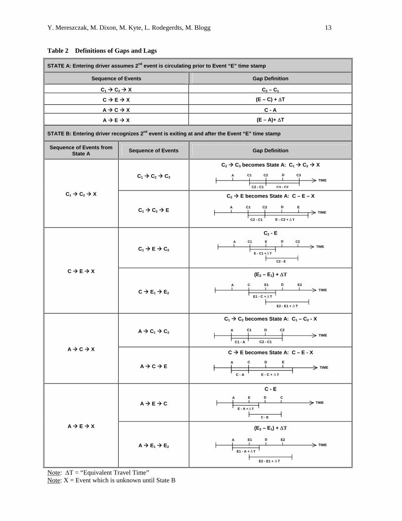
Definitions of Gaps and Lags
Tian (5) defines a gap event as a time stamp used to denote the beginning and/or end of each major stream gap. The size of the gap is the difference between the begin gap event and the end gap event. The priority stream, or major stream, is the stream of vehicles that can pass the approach without delay. This is usually assumed to be the circulating stream of vehicles for roundabouts. The minor stream is the stream of vehicles that can only enter the conflict area if the next major stream vehicle is far enough away to allow safe passage.
Tian (5) explains if a minor stream vehicle arrives subsequent to the passage of the begin gap event, the minor stream driver is encountering a lag rather than a gap. The size of the lag is measured from the time the minor stream driver arrives at the yield line until the passage of the end gap event or the next major stream vehicle. The begin gap event for a lag is the time at which the subject vehicle arrives at the yield line.
A general assumption in gap acceptance theory is that the gaps in the major stream, as perceived by the entering driver, remain unchanged. However, as shown by Hagring (2) in Figure 2, if Vehicle B exits then a new gap consisting of x1 + x2 arises. The major stream driver begins evaluating this new gap at the moment Vehicle B can be distinguished as exiting. This moment is often difficult to define, and that is why the exiting point is more like an exiting area (2). However, in most cases, this area is treated as if it were a single point (2). A similar methodology was used in this study for incorporating exiting vehicles in critical gap estimation.
Since the maximum likelihood technique was used as the method for estimating critical gaps, the exiting vehicles must be incorporated in a way that allows for the identification of a driver’s accepted and largest rejected gap. The logic for incorporating the exiting vehicles is outlined in Figure 3 and explained as follows.
Three vehicles traveling within the circulatory roadway at a single-lane roundabout are designated Vehicles A, B, and C. A minor stream vehicle (Vehicle D) has entered the service position, and is evaluating traffic in the major stream to determine whether it is safe to enter the roundabout (Stage 1 in Figure 3). If the entering driver perceives the first vehicle (Vehicle A) as circulating, and does not find adequate time to enter the roundabout ahead of this circulating vehicle, then the entering driver will begin to analyze the time to the next vehicle (Vehicle B). However, it may not be immediately apparent whether Vehicle B is circulating or exiting. The driver may or may not enter during the period when they are unsure of the future path of Vehicle B. This is shown in Stage 2 of Figure 3.
If Vehicle B exits, the entering driver will end evaluation of the time to this vehicle at the moment the driver recognizes Vehicle B is exiting. This moment is assumed to be when Vehicle B crosses a line extending out from the splitter island perpendicular to the flow of exiting traffic. This assumption is conservative, as exiting
Y. Mereszczak, M. Dixon, M. Kyte, L.Rodegerdts, M. Blogg 5
vehicles sometimes shy to the outside part of the circulatory roadway, and thus can be distinguished from circulating vehicles prior to exiting. In addition, some exiting vehicles use turn indications.
Stage 3 in Figure 3 shows that once Vehicle B crosses the exit point, the entering driver is no longer evaluating the gap between Vehicle A and Vehicle B. If the entering driver chose not to accept this gap, then the driver is now evaluating a new gap between the time that Vehicle B was recognized as exiting and the last vehicle (Vehicle C). The entering driver must now evaluate the future path of Vehicle C and whether or not there is sufficient time to enter before Vehicle C reaches the conflict point.
Equivalent Travel Time
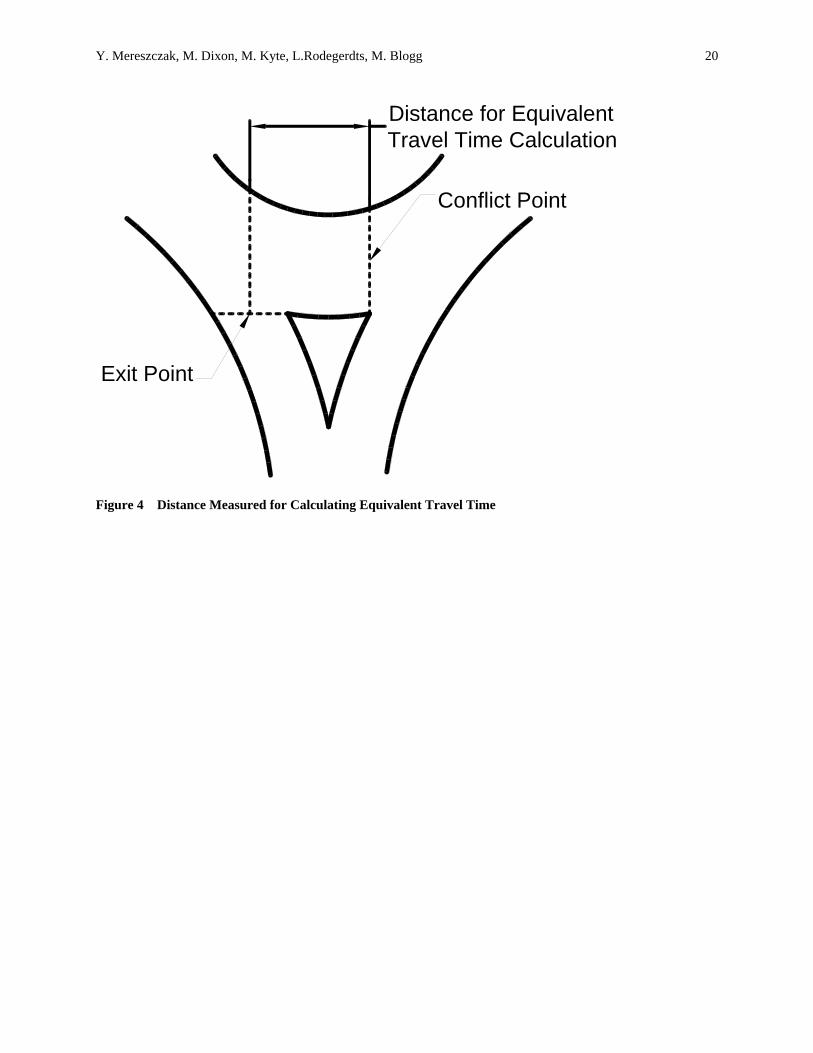
In order to compare gaps either partially or wholly comprised of exiting vehicles to gaps between two circulating vehicles, some amount of time must be added to particular gaps defined by exiting vehicles to accurately quantify the perceived headways. This added time will account for the travel time that would have occurred between the exit point and conflict point had the vehicle remained in the circulating flow. The amount of the added time is termed the “equivalent travel time”, and is calculated using a radar sample of average circulating speeds at each approach, along with measured distances from the exit point to the conflict point. Figure 4 is provided to illustrate the distance measured between the exit point and the conflict point.
Table 1 shows the equivalent travel times calculated for each approach. The equivalent travel time for an approach is added to gaps defined by a particular sequence of events as outlined in Table 2. It is worth mentioning that the equivalent travel time is not added to the time stamp of the exit event, as this would shift the occurrence of the event in time.
Assumptions
The process described above for defining gaps and lags with the incorporation of exiting vehicles implies three major assumptions:
• Each exiting vehicle would have traveled the distance between the exit point and the conflict point in exactly the equivalent travel time calculated for an approach.
• Each entering driver cannot distinguish the future path of a major stream vehicle prior to the exit point. • Each entering driver recognizes a major stream vehicle has exited at and after the major stream vehicle
crosses the exit point. Many drivers will not behave in exactly the manner described by these assumptions; however, these assumptions were observed to be reasonable, and are necessary in order to provide a consistent procedure for extracting gaps and lags from the data.
ANALYSIS
Critical Gap Estimation
Tian (5) explains that the maximum likelihood technique for estimating critical gap is based on the idea that a driver’s critical gap lies between his or her largest rejected gap and accepted gap. A lognormal distribution is most commonly assumed to represent the critical gaps. This distribution contains only non-negative values, since critical gap cannot be negative, and is skewed to the right because more drivers are likely to accept larger gaps.
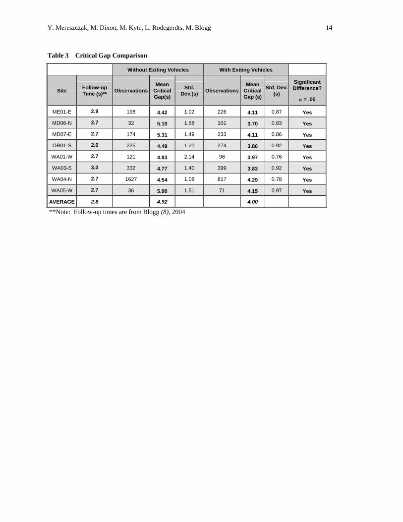
Table 3 presents the critical gap values estimated for each approach through the use of critical gap estimation software that applies the maximum likelihood technique (6). Only entering vehicles accepting a gap, also defined as those vehicles first rejecting a gap or a lag, were included in the critical gap estimation dataset. A rejected lag was treated the same as a rejected gap.
Comparison of the critical gap values shows a decrease at all approaches when exiting vehicles are incorporated. This observation is similar to the findings of Kyte et al., where the critical gaps estimated at TWSC intersections became smaller with increasing proportions of right-turn vehicles in the conflicting flow (7). The smaller critical gap estimates for TWSC intersections were attributed to the fact that the right-turn vehicles caused less conflict than the through vehicles (7). The smaller critical gaps for these study approaches may be attributable to a reduction in the size of many accepted and rejected gaps. Gaps between circulating vehicles, once containing one or more exiting vehicles, now are disaggregated into multiple gaps. Also, many lags are now defined by the presence of an exiting vehicle. This leads to an increase in the number of observed rejected lags, which are typically smaller than rejected gaps.
Y. Mereszczak, M. Dixon, M. Kyte, L.Rodegerdts, M. Blogg 6
A statistical analysis completed for each approach evaluated the significance of the difference between critical gaps determined both with and without the incorporation of exiting vehicles. The results are shown in Table 3. The difference is significant at the 95% confidence level for all eight approaches. This suggests that incorporating exiting vehicles significantly changes the perceived gaps that minor stream drivers choose to accept or reject.
Capacity Estimation and Comparison to Measured Field Capacities
As mentioned above, the critical gaps shown in Table 3 were determined for each approach both with and without the incorporation of exiting vehicles. Follow-up times at each approach were also extracted from the data and are displayed in Table 3. At each approach, the counts of circulating and exiting vehicles were collected over various lengths of time. The entire time period during which data were collected at each approach was divided into 15-minute sub-sections in order to achieve a larger sample size for capacity estimation.
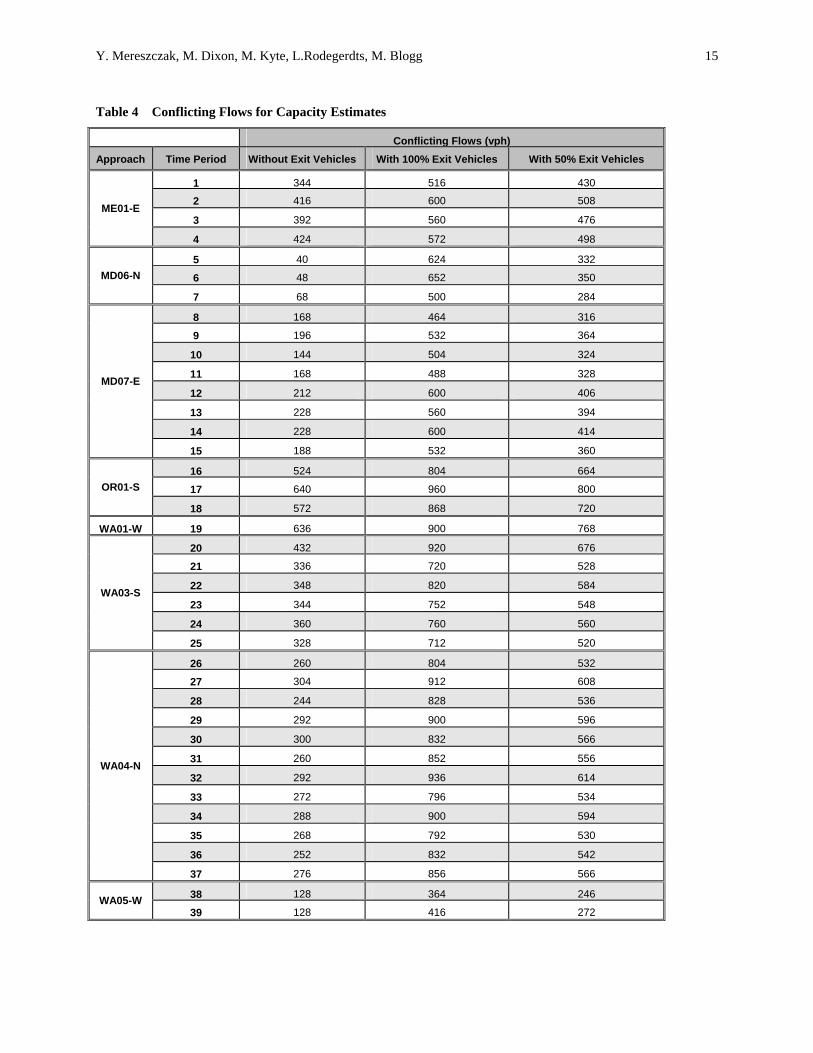
The hourly conflicting flow rate was estimated according to three different methods. The first method determined conflicting flow rate using the 15-minute circulating flow rate. These conflicting flow rates were used in the estimation of capacities without the incorporation of exiting vehicles. The second method determined conflicting flow rate using the 15-minute circulating flow rate plus 100% of the exiting flow rate. These conflicting flow rates were used in the estimation of capacities with the incorporation of 100% of the exiting vehicles. The third method determined conflicting flow rate using the 15-minute circulating flow rate plus 50% of the exiting flow rate. These conflicting flows were used in the estimation of capacities with the incorporation of 50% of the exiting vehicles.
Table 4 displays the estimated conflicting flow rates determined according to the three methods described above. For each 15-minute sub-section, the table displays the conflicting flow rates determined without exiting vehicles, with 100% of exiting vehicles, and with 50% of exiting vehicles. Equation 1 (HCM Equation 17-70) was used to predict capacity both with and without the incorporation of the exiting flow. The critical gaps estimated without exiting vehicles were used, along with the conflicting flow rates determined according to the first method, for predicting capacities without exiting vehicles. The critical gaps estimated with exiting vehicles were used, along with conflicting flow rates determined according to the second and third methods, for predicting capacities with 100% and 50% of exiting vehicles, respectively. The estimated follow-up times given by Blogg (8) were used in all instances of capacity estimation. Table 5 displays the capacities estimated without exiting vehicles, with 100% of exiting vehicles, and with 50% of exiting vehicles.
3600/
3600/
1 fc
cc
tv
tv
ca eevC −
−
−= 1
Ca = approach capacity (veh/hr) vc = conflicting flow rate (veh/hr) tc = critical gap (sec) tf = follow-up time (sec)
For every one-minute interval during each 15-minute sub-section the visually observed minutes of continuous queuing were identified. For each one-minute interval with a continuous queue, the entry flow rate was measured. All measured entry flow rates during a particular 15-minute period were averaged to provide a field capacity value, and a one-hour capacity was calculated assuming four equal 15-minute flows. These field capacity values were then compared to the capacity estimates with and without exiting vehicles.
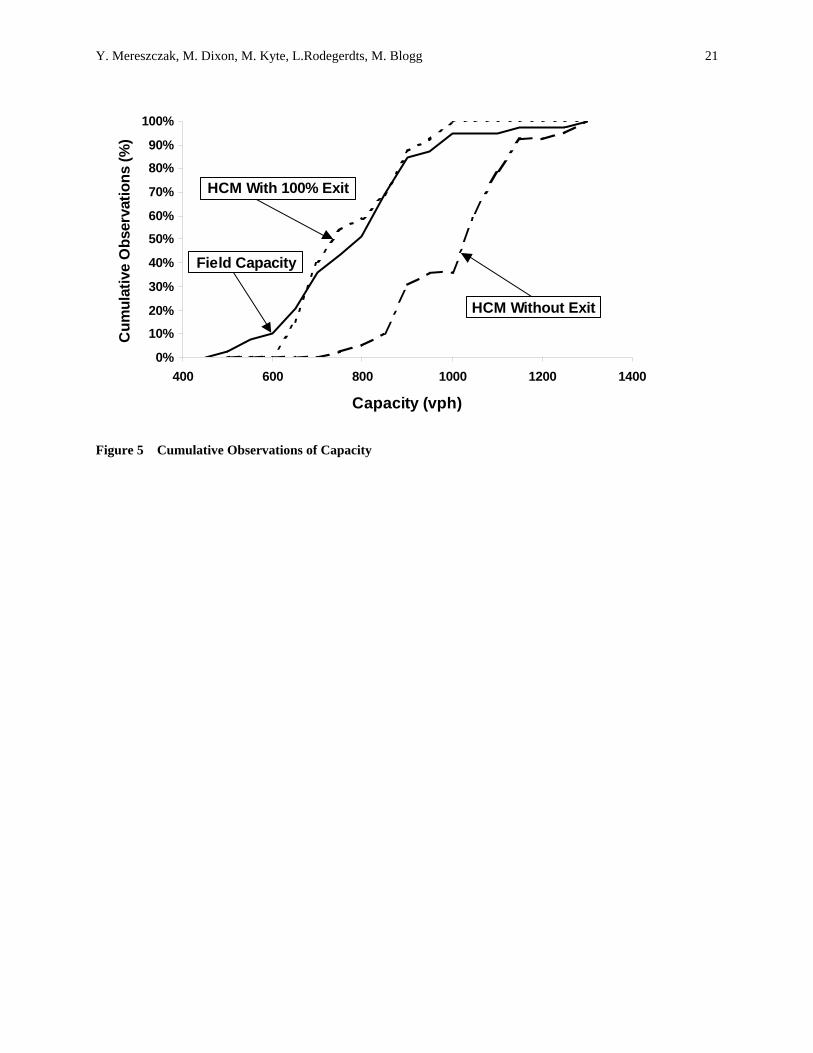
Figure 5 plots the cumulative distributions of the measured field capacities, the HCM capacity estimates without exiting vehicles, and the HCM capacity estimates with exiting vehicles. The curve representing estimates without exiting vehicles provides a distribution of estimates lying far to the right of the distribution of measured field capacities. The curve representing estimates with exiting vehicles provides a distribution that follows the measured field capacity distribution closely. The Kolmogorov-Smirnov test (K-S test) was performed to test whether the cumulative distribution of field capacities matches either of the estimated distributions. The null hypothesis was that the distribution of estimates matches the field distribution. For the distribution of HCM estimates without the incorporation of exiting vehicles, the null hypothesis was rejected at the α = .05 level (D = 0.59 > D.05 = 0.22). The conclusion is that the distribution of HCM estimates without the incorporation of exiting vehicles does not match the field distribution. For the
Y. Mereszczak, M. Dixon, M. Kyte, L.Rodegerdts, M. Blogg 7
distribution of HCM estimates with the incorporation of exiting vehicles, the null hypothesis was accepted at the α = .05 level (D = 0.10 < D.05 = 0.22). The conclusion is that the distribution of HCM estimates with the incorporation of exiting vehicles does match the field distribution. Based on visual inspection of Figure 5 and the results of the K-S test, HCM estimates with the incorporation of exiting vehicles result in improved estimates of the actual capacities of roundabout approaches.
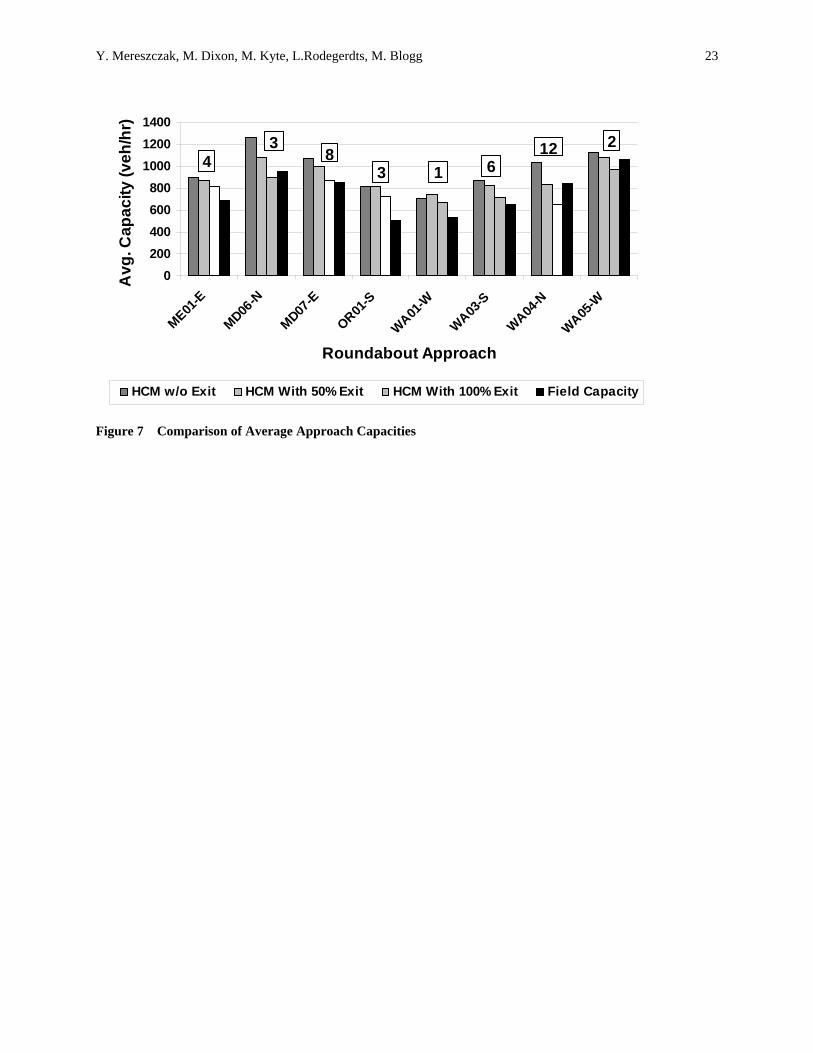
Figure 6 is provided to further support this conclusion, displaying the different capacity estimates versus the measured field capacities. The line represents estimates exactly predicting the measured field capacity. Nearly all capacity estimates without exiting vehicles lie above this line, indicating an overestimation of field capacity. Notice there are approximately an equal number of capacity estimates with exiting vehicles both above and below the line. An examination of the correlation of the capacity estimates without exiting vehicles to the exact prediction line yields an R2 value equal to 0.29. An examination of the correlation of the capacity estimates with exiting vehicles to the exact prediction line yields an R2 value equal to 0.57. This demonstrates that estimates with exiting vehicles have more explained variation relative to the exact prediction line than estimates without exiting vehicles. Therefore, the conclusion is that the field capacities are better explained by capacity estimates that incorporate exiting vehicles than by capacity estimates that do not incorporate exiting vehicles. Finally, Figure 7 provides a comparison of the average capacities from all time periods for each approach. The values listed above the columns represent the number of 15-minute sub-sections comprising the average capacity estimates and average field capacities for each approach. This figure reiterates the fact that HCM estimates without exiting vehicles overpredict the field capacities at all approaches. HCM estimates with 50% of exiting vehicles overpredict the field capacities at 7 out of 8 approaches. HCM estimates with 100% exiting vehicles overpredict the field capacities at 5 out of 8 approaches, but on average, fall much closer to the field capacities than either of the previous two estimates.
Explaining Capacity Prediction Errors
Troutbeck (9) found limited evidence of exiting vehicle effects at roundabout approaches in Australia, and stated that exiting vehicles should only be accounted for if circulating speeds are expected to be high, or if entering drivers fail to recognize differences in travel paths between circulating and exiting vehicles. From the previous section, it was determined that incorporating exiting vehicles improves capacity estimation at roundabout approaches; however, there remain some significant errors in capacity prediction. The second objective of this report is to explain these capacity prediction errors through the examination of particular geometric and flow parameters that govern entry and exiting vehicle interactions. Specifically examined in this report were the parameters proportion of exiting vehicles in the major stream and the width of the splitter island.
Proportion of Exiting Vehicles in the Major Stream
Figure 8 plots the mean percent error (MPE) between the capacity estimates and the measured field capacities against the associated proportion of exiting vehicles contained within the major stream of traffic. The mean percent error is defined as:
( )%100×
−=
field
fieldest
CCC
MPE
2
For the first comparison, 100% of the exiting vehicles were incorporated into the conflicting flow. Capacity was estimated according to Equation 1, and the MPE was calculated according to Equation 2. The indistinct linear trend of the MPE with exiting vehicles indicates that at lower proportions capacity is overestimated, while at higher proportions capacity is underestimated. There is no evident trend of the MPE without exiting vehicles; however, it is observed that nearly all MPE values are positive, indicating an overestimation of capacity at any proportion of exiting vehicles. Also, observe that as the proportion of exiting vehicles becomes larger, the MPE values between the two methods of estimation diverge. This suggests that as the proportion of exiting vehicles increases, the capacity predictions with and without exiting vehicles are deviating from each other.
In a study conducted at two-way stop-controlled intersections in the U.S. by Kyte et al. (7), minor street capacity prediction was improved by including 50% of right-turn vehicles from the major street in the conflicting flow. Further exploration of the MPE versus proportion of exiting vehicles was conducted to analyze the effects of only incorporating 50% of the exiting vehicles into the conflicting flow. Figure 8 plots the MPE for 50% and 100% incorporation of exiting flow against the associated proportion of exiting vehicles. The trend of the MPE with 50%
Y. Mereszczak, M. Dixon, M. Kyte, L.Rodegerdts, M. Blogg 8
of the exiting vehicles indicates that capacity is overestimated at any proportion of exiting vehicles. Note that at higher proportions, the MPE with 50% of the exiting vehicles is closer to zero percent than with 100% of the exiting vehicles. This leads to the conclusion that 100% of exiting vehicles should be incorporated into the conflicting flow unless an approach has a high proportion of exiting vehicles, in which case a lower percentage of exiting vehicles should be incorporated into the conflicting flow.
The idea that a lower percentage of exiting vehicles should be included at higher proportions may be an indication of driver expectancy. With fewer exiting vehicles in the major stream, drivers may be more hesitant to enter the roundabout prior to any vehicle in the major stream. With a high proportion of exiting vehicles, entering drivers may be less hesitant about entering the roundabout because they expect most vehicles in the major stream to exit. Further research should be conducted to support the above stated conclusion, and explore this relationship in more depth.
Width of the Splitter Island
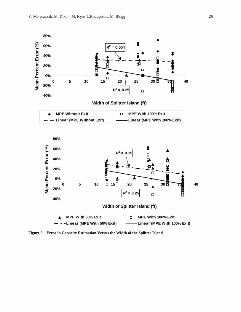
Figure 9 plots the mean percent error (MPE) between the capacity estimates and the measured field capacities against the associated width of the splitter island. For the first comparison, 100% of the exiting vehicles were incorporated into the conflicting flow. Capacity was estimated according to Equation 1, and the MPE was calculated according to Equation 2. The indistinct linear trend of the MPE with exiting vehicles indicates that at smaller splitter island widths capacity is overestimated, while at larger widths capacity is slightly underestimated. Also, observe that as the splitter island becomes wider, the MPE values between the two methods of estimation show a slight divergence. This suggests that as one moves from narrow to wide splitter islands, the capacity predictions with and without exiting vehicles are deviating from each other.
Further exploration of the MPE versus the width of the splitter island was conducted to analyze the effects of only incorporating only 50% of the exiting vehicles into the conflicting flow. Figure 9 plots the MPE for 50% and 100% incorporation of exiting flow against the associated width of the splitter island. The trend of the MPE with 50% of the exiting vehicles indicates that capacity is overestimated at any splitter island width. Visual inspection also suggests that capacity estimates with 100% of exiting vehicles more accurately predict the actual capacity than estimates with 50% of exiting vehicles. This suggests that for narrow splitter islands, 100% of exiting vehicles should be included in capacity estimation. For wider splitter islands, between 50% and 100% of exiting vehicles should be included in capacity estimation. Once again, further research should be conducted to support this conclusion and explore this relationship in more depth.
SUMMARY OF FINDINGS AND CONCLUSIONS
The current model used in the U.S. to predict approach capacity at single-lane roundabouts utilizes information about entering driver behavior in relation to the circulating stream of traffic only. No procedure is currently in place for incorporating exiting vehicles in capacity estimation. The primary purpose of this report was to determine if the incorporation of exiting vehicles results in improved prediction of entry capacity at a roundabout approach over capacity prediction with consideration for circulating vehicles only. This report also attempted to explain capacity prediction errors through the examination of particular geometric and flow parameters that govern entry and exiting vehicle interaction. Through the use of simulation, Hagring explained how accounting for exiting vehicles and their effects impacts approach capacity. He determined that capacity increases when the proportion of exiting vehicles is increased and the major stream flow is constant (2). This study expanded on the work of Hagring by providing an in-depth comparison of the capacity estimates, with and without exiting vehicles, to field measured capacities at approaches in the U.S. The conclusion was that the incorporation of exiting vehicles results in improved capacity prediction. It is of practical interest to note that an overall reduction in capacity prediction error of almost 20% is observed when exiting vehicles are included in the estimation process. It is recommended that exiting vehicles be accounted for in capacity estimation at U.S. roundabout approaches. Further research should be completed to identify the exact manner in which exiting vehicles should be incorporated.
Recall, both Troutbeck and Hagring found that exiting vehicles do have an effect on entry capacity, and they stated that this effect was most likely dependent on the geometry of the approach, major stream vehicle speeds, and the proportion of exiting vehicles in the major stream (2), (9). This study expanded on Troutbeck and Hagring’s observations by investigating errors in capacity prediction through the examination of the parameters proportion of exiting vehicles and the width of the splitter island. It was determined that these parameters provide some explanation of the prediction errors, but exactly how the parameters should be incorporated into the capacity prediction process needs to be further explored.
Y. Mereszczak, M. Dixon, M. Kyte, L.Rodegerdts, M. Blogg 9
ACKNOWLEDGEMENTS
The authors would like to thank the National Cooperative Highway Research Program (NCHRP) for sponsoring the research conducted in conjunction with this study. The authors would especially like to thank the Co-Principal Investigator Bruce Robinson for his leadership in the initial stages of the NCHRP 3-65 project, and data collection co-leaders George List, and Aimee Flannery for their contributions to organizing and managing the data collection process. The authors would also like to thank Ning Wu, Marais Lombard, and Lane Roberts for their data analysis contributions to this study, and Rod Troutbeck and Werner Brilon for their senior guidance. The authors would also like to thank Philip Rust, Hyunwoo Cho, Rebecca Brown, Stacy Eisenman, Alixandra Demers, William Johnson, and Angela Martin who, in addition to the authors, participated in the data collection efforts. Finally, the authors would like to thank Audra Sherman, Julia Busby, Brent Orton, Gary Haderlie, JoAnn Brazil, Chittemma Potlapati, and Christina Hemberry for their data extraction efforts.
Y. Mereszczak, M. Dixon, M. Kyte, L.Rodegerdts, M. Blogg 10
REFERENCES
1. Transportation Research Board, Highway Capacity Manual, Chapter 17 – Unsignalized Intersections, Committee on Highway Capacity and Quality of Service, Subcommittee on Unsignalized Intersections, Washington, D.C., 2000
2. Hagring, O., “Derivation of Capacity Equation for Roundabout Entry with Mixed and Circulating and Exiting Flows”, Transportation Research Record 1776, Transportation Research Board, Washington, D.C., 2001, pp. 91-99.
3. Troutbeck, R.J., “Does Gap Acceptance Theory Adequately Predict the Capacity of a Roundabout”, Proceedings 12th ARRB Conference, Vol. 12, Part 4, 1985, pp. 62-75.
4. Rodegerdts, L., Blogg, M., Kyte, M., Brilon, W., Wu, N., Troutbeck, R., Dixon, M., Draft: Operations Analysis Working Paper, Draft Report: Applying Roundabouts in the United States, National Cooperative Highway Research Program 3-65, Transportation Research Board, Washington, D.C., 2005
5. Tian, Z., Vandehey, M., Robinson, B., Kittelson, W., Kyte, M., Troutbeck, R., Brilon, W., “Implementing the Maximum Likelihood Methodology to Measure Driver’s Critical Gap”, Proceedings of the Third International Symposium on Intersections Without Traffic Signals, Portland, Oregon, 1997, pp. 268-73.
6. Troutbeck, R.J., Critical Gap Estimation Software, Queensland University of Technology, 2001. 7. Kyte, M., Tian, Z., Mir, Z., Hameedmansoor, Z., Kittelson, W., Vandehey, M., Robinson, B., Brilon, W.,
Bondzio, L., Wu, N., Troutbeck, R., Capacity and Level of Service at Unsignalized Intersections, Final Report: Volume 1 – Two-Way Stop-Controlled Intersections, National Cooperative Highway Research Program 3-46, Transportation Research Board, Washington, D.C., 1996
8. Blogg, M. , Estimation of Critical Gap and Follow-up Time, Draft Report: Applying Roundabouts in the United States, National Cooperative Highway Research Program 3-65, Transportation Research Board, Washington, D.C., 2004
9. Troutbeck, R.J., “Traffic Interactions at Roundabouts”, Proceedings 15th ARRB Conference, Vol. 15, Part 5., 1990
Y. Mereszczak, M. Dixon, M. Kyte, L.Rodegerdts, M. Blogg 11
LIST OF TABLES AND FIGURES
Table 1 Roundabout Approaches .............................................................................................................................12 Table 2 Definitions of Gaps and Lags ......................................................................................................................13 Table 3 Critical Gap Comparison .............................................................................................................................14 Table 4 Conflicting Flows for Capacity Estimates...................................................................................................15 Table 5 Capacities ....................................................................................................................................................16 Figure 1 Location of Collected Time Stamps...........................................................................................................17 Figure 2 Process of Exiting Vehicles – From Hagring (2), 2001 ............................................................................18 Figure 3 Methodology for Incorporating Exiting Vehicles in Gap Definitions .......................................................19 Figure 4 Distance Measured for Calculating Equivalent Travel Time .....................................................................20 Figure 5 Cumulative Observations of Capacity........................................................................................................21 Figure 6 Capacity Estimates Compared to Measured Capacities .............................................................................22 Figure 7 Comparison of Average Approach Capacities ...........................................................................................23 Figure 8 Error in Capacity Estimation Versus the Proportion of Exiting Vehicles..................................................24 Figure 9 Error in Capacity Estimation Versus the Width of the Splitter Island .......................................................25
Y. Mereszczak, M. Dixon, M. Kyte, L.Rodegerdts, M. Blogg 12
Table 1 Roundabout Approaches
Approach Label Intersection City State Equivalent
Travel Times (s)
WA05-W NE Inglewood Hill / 216th Ave NE Sammamish WA 1.3
WA01-W SR 16 SB Ramp / Burnham Dr Gig Harbor WA 1.7