1

Increasing the Capability of Neural Networks forSurface Reconstruction from

Noisy Point CloudsAdam R White, Li Bai

School of Computer ScienceUniversity of Nottingham

Jubilee Campus, Nottingham NG8 1BB, UK

Abstract—3D modeling from point cloud data is not exclusivelyin the vein of aesthetics but industrial products and medicalscanners. With the emergence of technologies like VR, and thereducing cost of personal laser scanners, the need for algorithmsthat give realistic representation of scanned data is ubiquitous.This paper builds upon the current methods to increase theircapability and automation for 3D surface construction fromnoisy and potentially sparse point clouds. It presents an analysisof an artificial neural network surface regression and mappingmethod, describing caveats, improvements and justification forthe different approach.

I. INTRODUCTION

Accurate surface reconstruction from noisy point clouddata is still an unsolved challenge. Raw point cloud data isunstructured and may be noisy or sparse. The challenge canbe tackled with a neural network (NN) approach [2], to learna mapping from a 2D parameterisation of 3D point clouddata, resulting in a surface that is less sensitive to noise.This approach differs to standard NN applications as boththe hyperparameters and intrinsic parameters change duringtraining in order to find the optimum model [2].

This paper considers the 2D parameterisation method, di-rectly comparing the current dimension reduction used andother familiar methods. A least squares Spline fitting is appliedto define and interpolate the boundaries of the surface mesh.The interpolants are carefully chosen by a method presentedto enable a fit that is more faithful to the boundary of objects.A working implementation is demonstrated, producing goodquantitative and qualitative results on a range of noisy datasets.

II. RELATED WORK

An approach was suggested by Peng et al [12] using animage processing inspiration for surface de-noising. It removesnoise by applying a Weiner filter which approximates thecomponents of the surface as a statistical distribution. Thereare two problems with this algorithm in our context. First, itneeds to be decided when this algorithm should be applied,unnecessary smoothing might remove features that describethe underlying geometry, although there is some attempt toapply a surface based anisotropic diffusion to preserve edges.In addition, the formula used requires the user to both knowand supply the noise denoted by the variance σ2 [12]. It may

not be possible to determine the noise of the data as it is anunstructured point cloud.

Mederos et al attempts to find local approximations ofimplicit surfaces on an object which is then combined into aglobal description [3]. This algorithm uses an octree to recur-sively divide the input space according to an error measuredat a node. With Machine Learning in context an interestingmethod was proposed where the knot vectors and controlpoints of B-spline curves and surfaces are learned [7].

Yumer and Kara suggest a NN regression method of sur-face fitting and hole stitching. The flexibility achieved byan adaptive neural network topology differs from previousattempts as the ideal topology of the network obtained (thehyperaparmeters) are not fixed [2], meaning the network canbe tailored to each point cloud automatically. This method isgood for removing noise as the underlying geometry of thepoint data and not random noise is represented in the finalsurface.

In a slightly different problem, where a NN is used toreconstruct the shape of a 3D object from its shading in a2D [6]. Khan et al show from experiment that quantitativeimprovement does not necessarily lead to quantitative im-provement. This is something to consider when using a ’blackbox’ function like a neural network, especially where therecould be some information loss. In this regard we must ensurethat the final model is representative of the ground truth andnot only rely on an error measure. It is suggested that moreresearch must be done for 3D surface quality metrics [6].Visual quality will be assessed in the method presented herealongside quantitative results in the absence of quality metrics.

Many papers in the field use a least squares based optimi-sation to curve or basis fitting [27] [13], [23] to cite a few.Wang et al (2006) admits that this automated fitting is still aproblem in graphics [27]. They introduce a direct SD squareddistance error function which is iteratively updated by usingquasi-Netwon gradient descent. The spline in this case has aninitial shape which is fit to the point cloud by taking the 1storder derivative of the objective function. The method usedin their paper assumes the knots are fixed in place [27]. Themethod chosen for our research allows variable knots as thisallows for a better fit and flexibility of model [23]. Despitethis constraint the paper shows excellent empirical results andwould have been tested had an implementation been readily

arX

iv:1

811.

1246

4v2

[cs

.GR

] 3

Dec

201

8

2

available for the programming language used for this paper.A recent development is the use of Spherical Harmonics for

Modeling where a surface can be described by three sphericalfunctions based on a bijective between the Cartesian (x,y,z)and (θ, γ) the spherical domain [16]. The method by Caitlinet al [13] transform mesh vertices into spherical coordinatesand use a form of Tikhonov regularisation to create a smoothmesh of the surface. While our solution does not take the sameform, we consider a smoothing criteria similar to Caitlin et al(2015).

III. MATERIALS AND METHODS

We aim to create an accurate surface from noisy point clouddata by analysing and improving a NN approach by [2]. Thesteps required to achieve goal of this paper are:

1) Use the Isomap algorithm to reduce the dimensions ofthe point cloud R3 → R2

2) Train NN to map R2 → R3. This mapping learned bysampling the initial point cloud and using the points astraining and test data.

3) Use a multi-depth path method to choose the outer-mostpoints of the 2D manifold to be interpolated

4) Least Squares fit a cubic B-spline to the interpolantschosen with a justifiable choice of regularisation

5) Re-sample points inside of the boundary dictated by B-spline

6) Find the triangular tessellation of the point cloud byDelaunay triangulation

7) Feed NN the points in R2 to produce the target verticesin R3

8) Mesh output according to triangular topology producedin R2

A. Feature Selection and Dimensional Reduction

The purpose of dimension reduction in this case is to allowa NN to learn a mapping between the 2D coordinates and the3D coordinates [2]. Also, it simplifies the problem of surfacegeneration: The boundary of the point set can be easily definedin 2D and the topology of the mesh established. Later thevertices of the mesh are fed to a trained NN.

The first step of the proposed algorithm is to embed thepoints in R3 to R2. Our feature space will only ever beR3, as is intrinsic to generating 3D surfaces in Euclideanspace. To facilitate the 2D embedding the use of Isomapalgorithm is suggested, originally proposed by Tenenbaum etal in 2000 [19]. The holistic reason for using Isomap over otherdimension reduction algorithms is because Isomap intends topreserve global geometry [19]. Given the goal is to extractthe underlying geometry and not the noise of the point cloudto produce a smooth surface, the 2D embedding must berepresentative.

The hallmark of Isomap is that points are reconstructedaccording to their pairwise geodesic distance. A graph foreach neighborhood is used to represent the distance pathwhere each edge is weighted, usually by euclidean distance.A neighborhood is defined by either by K points or a radiusdenoted by σ.

1) Determination of neighborhood for each pair of pointsj,i is given by dx(i, j) and store relations as a weightedgraph G.

2) Compute the shortest path distance dG(i, j) using analgorithm such as Floyd-Warshall.Once the graph distances are obtained as matrix DG =dG(i, i) the Multi-dimensional Scaling algorithm is ap-plied.

3) Finally the coordinate vectors in the resulting space Yare reconstructed to reduce the cost function:

E = ||τ(DG)− τ(DY )||L2 (1)

from [19] DY represents the matrix of Euclidean distances.τ converts the distances to inner products

B. Comparison

1) Qualitative Comparison: To make our investigationmore critical we compare Isomap and Locally Linear Embed-ding (LLE) [2]. Silvia and Tenenbaum, the original authorsbehind Isomap, published a comparison between Isomap andLLE two years earlier. In the defence of LLE it was suggestedthat it would be useful on a broader range of data when thelocal topology is close to Euclidean [10]. LLE is attractivein this regard as many surfaces to be produced will havelocal geometry that is close to Euclidean. We also desire arepresentative 2D embedding that is conducive to an accurateoutput once input to the learned NN. When noise is present itis more important that the general structure of the point cloudis learned and not the noise. Global methods, like Isomap,tend to give a more ’faithful’ representation with respect to itsglobal geometry [10]. With two algorithms, and two desiredproperties, we attempt to evaluate (and decide on the best)applicability to the niche problem in this section.

Fig. 1. Isomap with 12 nearest neighbors

3

Fig. 2. LLE modified weight method [22] 12 nearest neighbors

Before a surface was constructed we compared the outputof the trained NN against the original data (the StandfordBunny point cloud with 1600 points) to ascertain which twodimensional input gives us results closest to the original. Allmethods gave expected results on a more complex and densepoint cloud. The Hessian eigenmap method by Donoho andGrime [21] performs poorly on capturing the relative scale ofthe ears. The modified weight [22] LLE method seems to givethe most intuitive results.

2) Quantitative Comparison: We conducted further sys-tematic tests to distinguish the proper use of either a globalgeodesic method like Isomap or the Modified LLE. In orderto ensure results weren’t reflective of a particular datasetor neural network topology, all combinations of activationfunctions from a pool of well known functions were chosenand tested.

The size constraints of the network were kept relativelysmall to account for a lengthy training+test run time.

Both methods are dependent on the activation functions andboth methods give similar qualitative results as error. However,it became apparent that a second unintended independentvariable, being the cardinality of the points in the data set,affects the final NN output error for different methods of 2Dembedding. The results show that the Modified LLE methodhas the edge for very sparse data whereas Isomap gave betterresults on denser (relatively speaking) datasets. Modified LLEoften failed to run at all on dense datasets and we havediscounted the traditional method of LLE especially givenits non deterministic output. Therefore, from the experiments

IO layers Method K MSE rSigmoid Isomap 12 0.001503Sigmoid Mod LLE 12 0.001483Linear Isomap 12 0.0003200Linear Mod LLE 12 0.0004637

Fig. 3. All other constraints on the neural network: epochs, max layers, maxneurons were fixed.

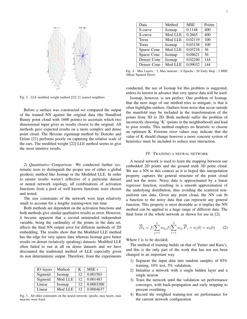
Data Method MSE PointsS-curve Isomap 0.1148 400S-curve Mod LLE 0.2665 400Torus Mod LLE 0.02119 100Torus Isomap 0.03138 100Sparse Cone Mod LLE 0.03218 36Sparse Cone Isomap 0.04621 36Denser Cone Isomap 0.02240 144Denser Cone Mod LLE 0.09032 144

Fig. 4. Max Layers : 3, Max neurons : 6 Epochs : 20 Early Stop : 3 MSE(Mean Squared Error)

conducted, the use of Isomap for this problem is suggested,unless its known in advance that very sparse data will be used.

Isomap, however, is not perfect. One problem of Isomap,that the next stage of our method tries to mitigate, is that itoften highlights outliers. Outliers from noise that occur outsidethe manifold may be included in the transformation of thepoints from 3D to 2D. Both methods suffer the problem ofincorrectly choosing ’K’ (points in the neighborhood) and leadto poor results. This method employs no heuristic to choosean optimum K. Extreme error values may indicate that thevalue of K should change however a more concrete system ofheuristics must be included to reduce user interaction.

IV. TRAINING A NEURAL NETWORK

A neural network is used to learn the mapping between ourembedded 2D points and the ground truth 3D point cloud.We use a NN in this context as it is hoped this interpolationproperty captures the general structure of the point cloudand not the noise. Noisy data is approximated by a linearregressor function, resulting in a smooth approximation ofthe underlying distribution, thus avoiding the scattered non-uniform raw data. Given any point cloud, the NN can fita function to the noisy data that can represent any generalfunction. This property is most desirable as it implies the NNmethod can be applied to a huge range of different data. Thefinal form of the whole network as shown for use in [2].

−→Dk = f(

n∑j=1

wkjf(

2∑i=1

wji−→P i + wj0) + wk0) (2)

Where f is to be decided.The method of training builds on that of Yumer and Kara’s,

and this is the only part of the work that has not not beenchanged in an important way.

1) Segment the input data into random samples of 85%training, 10% test, 5% validation,

2) Initialize a network with a single hidden layer and asingle neuron

3) Train the network until the validation set performanceconverges, with back-propagation and early stopping toprevent overfitting

4) Record the weighted training-test set performance forthe current network configuration

4

5) Increase the number of hidden neurons by 1. Iteratesteps 3-5 until the weighted performance converges orthe number of neurons reaches a maximum

6) Record the number of neurons and the test performancefor the current layer

7) Iterate steps 3-7 until the number of layers reaches amaximum

8) Return the network configuration with the best weightedperformance

[2]

V. SURFACE GENERATION

A. Defining the manifold

Once the point set is embedded in two dimensions thenext task is to sample the edge points of the now 2D pointcloud and fit an curve to define the manifold. Once the 2Dvertices generated by the procedure are fed to the trained NNthe resulting points in 3D represent less noisy version of theintended surface. The output points of the NN become verticesof a triangular mesh.

Prior research makes the assumption that the boundary pointset of the 2D embedding is a reasonable outline of the expectedshape, but with very noisy data outliners outside the expectedboundary would still be considered as valid points, causing themanifold to appear perturbed. We use the idea of re-samplingthe inner points with a regular grid, based on Yumer and Kara’swork [2]. The method chosen here is outlined below. It makesno assumptions about the quality of the boundary points andcan handle outlier points not representative of the manifold.

1) Sample a proportion of the outer most points in thecloud using the multi-line sampling method describedin ’Choosing the Interpolants’

2) Use sampled points to fit a cubic B-spline curve usingLeast Squares fit with regularisation [23]

3) Superimpose regular grid on point set and uniformly re-sample points inside of B-spline loop

In order to represent the outline of the 2D point cloud weuse a cubic B-spline curve to better fit the local boundary ofthe dataset [15]. The B-spline is defined as follows:

Si(t) =

3∑r=0

Pi+rBkr (t) for 0 ≤ t ≤ 1 (3)

where r denotes blending ratio and k the degree of theBernstein basis

B1i =

(t− ti

ti+1 − ti

)+

(ti+2 − t

ti+2 − ti+1

)(4)

when ti ≤ t ≤ ti+1 the Berstein basis and associated controlpoint blend in.when ti ≤ t ≤ ti+2 the control point and Bernstein basisblend out.

The task of deciding which pi control points, the sequenceof values for ti (knot vector) and additional weights thatinterpolate the points best will be discussed in surface fitting.

B. Choosing the interpolants

For the purposes of fitting the B-spline we are reducing theproblem to a Least Squares interpolation, and the interpolationis only as good as the interpolants are representative. In similarwork it was suggested that the outermost path connected by4 corners by polyline [2]. This works just fine for relativelynoise free data but it became apparent that the method can beimproved for noisy data sets and made more precise for non-noisy data. We can not use a 1-point deep outer loop as theprobability of this being true to the noise free representationof the surface outline is very low. With the addition of thenoise, the outer-loop will very likely be perturbed. However,unless the points do not even remotely resemble the expectedgeometry, we do know that somewhere between the outer mostpoints and a few points in the centroid direction lies the outlineof the ’perfect’ noise free shape.

• For each depth• Pick 8 (or more if desired) corners according the furthest

distance in circular sector from the centroid• For each corner

– Segment point space into rectangles containing allpoints between one corner and its adjacent corner

– Consider points between as weighted graph (usingKDTree in this case)

– Set weights to be w = c1.ds + c2.dc where ds, dcare the straight line distance to adjacent point andcentroid, respectively. c defining the ’importance’

– Find the shortest path to adjacent point using w ascriteria for next point selection

• Strip path containing selected points away from cloud soas not to be calculated for next depth

• Combine path returned for all corners

This method differs from previous attempts as more ’anchor’points are selected according to the spoke sampling criteriamentioned earlier. The incorporation of more anchor pointsgave better local precision for finding a path as the distance,and thus points considered between each anchor, ensures thealgorithm has less room for error: by a short circuiting path,for example. Further, our method allows adjustable depth ofpoints to be sampled so more interpolants can be consideredwhen fitting a boundary.

Fig. 5. Our Multi-depth bath-based sampling with noise (left). Polylinesamples with PCA corners similar to [2] (right) You can see how easily thesecond method is susceptible to noise. Even if re-sampled.

5

C. Surface fitting

In order to fit the spline to the selected interpolants we useDierckx’s algorithm for least squares fitting a B-spline withvariable knot vectors. Where the knot vector is a vector ofinitial values for the ’blending ratio’ and define the amountof ’blending’ for each control point on the curve (equation 8).The general form of the least squares for the fitting a B-splineis arranged by Dierckx as:

δ =

m∑r=1

(wryr −

g∑i=−k

piwrBk+1i (xr)

)2

(5)

from [23]• data points: (xr, yr)• set of weights wr

• the control points pi• the number an position of the knots t• substitute the blending ratio and Bernstein basis ’Bk

i ’from (4).

We have only shown a system where the knot vectors arefixed. Here, we will keep the description for picking theappropriate knots brief and suggest readers seek [23] for amore vigorous explanation. Dierckx avoids the problem ofcoinciding knots, and the existence of knots very near to thebasis boundary [a,b], by separating (3) the least squares splineobjective function and penalising the overall error using thefollowing heuristic.

ε(t) = σ(t) + pP (t) (6)

from [23] where p is not to be confused with a control pointand is set according to some heuristic

P (t) =g∑

i=0

(ti+1 − ti)−1 (7)

from [23] It’s plain to see that the penalty is inverselyproportional to the ’closeness’ of two adjacent knots. Due tolocal stopping points on the boundary [23] these constraintshelp avoid poor gradient based minimisation.

With the residual error σ from equation 5. Dierckx suggeststhe objective function can be subject to the constraint thatσ ≤ s where s is a user selected constant [23]. This allows theerror function some flexibility so that the spline is not forcedto traverse every point exactly. For the agenda of this paper asmooth fit is highly desirable. To this end, we attempt to buildupon the smoothing property introduced by Dierckx. Pickingthe value of ’s’ is the most challenging task. While there existssome heuristics to setting ’s’ before fitting the spline, therewas improvement on setting an arbitrary regularisation termby using the variance of y values in the target point set.

δ ≤ λ∑n

i (yi − y)2

|y|(8)

Given that we want a curve that smoothly traverses theinterpolants, the rationale behind using the variance is thatthe larger the discontinuity of values the greater allowance forfitting error thus the smoother the fit for jagged interpolants.

λ is set at a default value but can be tweaked should the userdesire. The pit fall with this method is that different values oflambda can still be tailored to each dataset thus the selection ofthe regularisation is not a fully automated process for findingthe optimum qualitative results.

One problem with triangulation algorithms is that they arenot well suited to concave point clouds and cause edgesoutside the outer loop of the points to be created. Currentlythe working implementation for surface generation uses a basicmethod for removing triangles outside of the boundary definedby the fitted B-spline. The algorithm simply:

• Compute the centroid of each triangle in the triangulation• Consider spline as polygon loop which encompasses all

correct triangulations by centroid• Triangles with centroids that exist outside of B-spline

polygon are removedNote that this method assumes that an optimal regularisationterm has been picked otherwise jagged and overfit boundarieslead to the removal of triangles that would contribute to gooddefinition of the surface.

VI. RESULTS AND OBSERVATIONS

The implementation is written in python and has 3 maindependencies: Pybrain, Sklearn [29] and Matplotlib.

We show the effect of using a retrained network verses acopy of the best network found in training. If ’Retrained’ is’Yes’, this indicates that a new NN was trained on all thedata available after the best topology was discovered duringtraining. If ’Retained’ was ’No’ then an exact copy of thetrained network with the best topology during training wasused on the whole data set. ’Final Error’ reflects the meansquared error of the network output given the whole data setas an input and not just random samples. Its worth noting thatthe error in this case is compared against the noisy data so avery low error can mean that the points have overfit to thenoise. It should also be noted that this wasn’t the case for theearlier results in the ’dimensionality reduction comparison’section, where the error was defined against the ’perfect’error free parametric representation of the intended object.

Overfitting on the test data needs to be avoided as it is theoverall structure of the geometry that must be captured, andthe test set, while sampled randomly, will skew the Final Errorif we allow the NN to overfit. The initial preconception thata retrained network, with optimum hyperparameters, wouldperform better. Having been trained on the whole data setan expected a closer representation of the ground truth, butexperimentation shows that a larger number of epochs causesthe error of the retrained NN to diverge from the improvementshown by the other non-retrained NNs.

6

Fig. 6. 1) PCA polyline sampling, 2) Spoke-like sampling, 3) Sampling method used in this paper

Fig. 7. Deep Learning potential attempted with 20 neurons max per layer. λ = 2.4

The quality of the boundary of the point cloud directlyaffects how perturbed the resulting tessellation will appear onthe final output. We will compare other methods of choosinginterpolants and show the importance of having more pointsafforded to interpolation by allowing a variable depth of sam-ples that form the outer loop. In order to keep the independentvariables limited to 1, and to show the problem in a simplemanner, the following images show the least squares fit of aBezier curve for simple points sets. This is the same processas [2] - what changes is the sampling method:

VII. CONCLUSION

Discussed in this paper is the methods for surface generationfrom noisy point cloud data. Through experimentation wehave been able to expose the internals of the algorithmssuggested, and give a closer comparative review of this highlyspecific application of neural networks. The presented methodgives good quantitative and qualitative results for a variety ofdifferent data sets. With a little more refinement, particularlyin the training of the NN, it is hoped that this method can beextended for more complex 3D point clouds.

A software improvement which will speed up the trainingtime of the neural network is the use of a more modernlibrary than Pybrain. On top of this, a better training method

7

Dim Reduction NN layers NN neurons Epochs Train Error mse Final Error mseIsomap 1 6 100 0.006328 0.000798LLE (original) 1 10 100 1.429 0.296

Fig. 8. for θ = [0..π2], γ = [0..π

2] on Torus

Dim Reduction NN layers NN neurons Epochs Test Error mse Final Error mse RetrainedLLE 1 10 10 0.9102 1.071 YesLLE 2 (10, 6) 100 0.5376 1.212 YesLLE 3 (10,10,1) 10 0.7643 1.130 NoLLE 2 (10,2) 100 0.3519 0.7654 NoLLE 2 (10, 4) 100 0.7191 0.6382 No

Fig. 9. for θ = [0..π], γ = [0..π] on Torus

should be used to reduce training time. Currently, the trainingmethod is simply a gradient descent backpropgation. Not muchattention has been payed to parameters like the momentumupdate, learning rate and other hyperparameters. It would beprudent to refine the method of training as this will be theslowest part of the algorithm. While most of the datasets andneural networks in this, and other papers [2], are constrained tosmall manageable sizes. The potential for larger, that is deep,with many layers defined in [28], should not be overlookedfor complex mappings. However, this is only feasible in areasonable time frame if the selection of the hyperparamtersis more efficient than an exhaustive grid search, otherwisesegmentation of the problem will need to be employed.

Finding the best regularisation value should be also be onthe agenda for improvement. The regularisation parameter,while manifold specific, is fixed throughout the fitting ofthe B-spline. Ideally there need to some variability in theamount of regularisation at the moment of update of leastsquares. It would be good to the follow a ridge regressiontrend in further implementations of this algorithm where theregularisation can be more closely dependent on the splinebeing fit in a similar way as Caitlin et al use the sphericalharmonic order to construct the Tikhonov matrix [13]. Asmentioned, regularisation strongly affect the qualitative resultsand currently a free parameter lambda exists that is notautomatically decided.

There needs to be some decision towards when hole fittingis appropriate. This method will blindly re-sample the insideof the point cloud whether or not holes where intended. To beable to realise more complex surfaces with intentional holessegmentation could be used but this immediately increase thecomplexity of the algorithm. To find a global method whichfills in only unintended holes is a very challenging task butwould improve this algorithm.

REFERENCES

[1] FABIO.R (2004) From Point Cloud To Surface: The Modelingand Visualization) Problem[Online]. International Archives of Pho-togrammetry, Remote Sensing and Spatial Information Sciences. Vol34. ppg1,4. Available at http://www.isprs.org/proceedings/XXXIV/5-W10/papers/remondin.pdf [Accessed 21/10/2017]

[2] YUMER.M and KARA.L (2011) Surface Creation onUnstructured Point Sets Using Neural Networks[Online],Pittsburg, Carnegie Mellon University, Available at:vdel.me.cmu.edu/publications/2012cadp1/paper.pdf [Accessed23/10/2017]

[3] MEDEROS.B, LAGE.M, AROUCA.S, PATRONETTO.F, VELHO.L,LEWINER.T and LOPES.H. (2007) Regularized implicit surface recon-struction from points and normals J.Braz.Comp.Soc. [Online], vol.13,n.4, pp.7-16. Available at: http://www.scielo.br/pdf/jbcos/v13n4/02.pdfppg 1, 10 [Accessed 23/10/2017]

[4] BERNARDINI.F and RUSHMEIER.H (2002) The 3D model AcquistionPipeline, New York, IBM Thomas J. Watson Research Centre, [Online],vol 21, n.2, pp.149-172 Available at : www1.cs.columbia.edu/ allen/PHOTOPAPERS/pipeline.fausto.pdf [Accessed 25/10/2017]

[5] ISSELHARD.F, BRUNNETT.G, SCHREIBER.T (1998) Polyhedralapproximation and first order segmentation of unstructured pointsets[Online] IEEE 433 - 441. 10.1109/CGI.1998.694297. ppg 1,9 Avail-able at http://ieeexplore.ieee.org/document/694297/ [Access 26/10/2017]

[6] KHAN. N, TRAN. L, TRAPPEN. M (2009). Training many-parametershape-from-shading models using a surface database. 2009 IEEE12th International Conference on Computer Vision Workshops, ICCVWorkshops 2009. 1433 - 1440. 10.1109/ICCVW.2009.5457444. ppg 7[Accessed 21/09/2017]

[7] VAN TO.T and KOSITVIWAT.T (2005) Using Rational B-SplineNeuralNetworks for Curve Approximation[Online] MATHEMATICALMETHODS and COMPUTATIONAL TECHNIQUES INELECTRICAL ENGINEERING, Sofia, 27-29/10/05 (pp42-50)Available at https://www.researchgate.net/publication/255599876 Using Rational B-Spline Neural Networks for Curve Approximation [Accessed27/11/2017]

[8] SHALIZI. C (2009) Nonlinear Dimensionality Reduc-tion I: Local Linear Embedding[Online] Available at:http://www.stat.cmu.edu/ cshalizi/350/lectures/14/lecture-14.pdf ppg1-3[Accessed 03/12/2017]

[9] ROWEIS. S.T, SAUL. L.K, (2000) Nonlinear dimensionalityreduction by locally linear embedding. [Online], Science(New York, N.Y.) 290 (5500) 23236. Available at:https://www.cise.ufl.edu/class/cap6617fa15/Readings/Science-2000-Roweis-2323-6.pdf [Accessed 28/11/2017]

[10] SILVIA. V.D and TENENBAUM. B. J (2002) Global versus local meth-ods in nonlinear dimensionality reduction[Online]Advances in NeuralInformation Processing Systems. 705-712Available at: http://web.mit.edu/cocosci/Papers/nips02-localglobal-in-press.pdf ppg1-2[Accessed 04/12/2017]

[11] BISHOP. C.M (2006) Pattern Recognition and Machine LearningSpringer Science+Business Media New York ppg 227

[12] PENG. J, STRELA. V. ZORIN.D (2001) A Simple Algorithmfor Surface Denoising[Online]Proceedings of the IEEE Visual-ization Conference. . 10.1109/VISUAL.2001.964500. Available athttp://www.mrl.nyu.edu/ dzorin/papers/peng2001sea.pdf ppg [Accessed06/12/2017]

[13] CAITLIN R. N, WIL 0.C. W, BARTOSZ P.N, LI. B Spherical Harmon-ics for Surface Parameterisation and Remeshing [Online] MathematicalProblems in Engineering Volume 2015, Article ID 582870 Available at:http://dx.doi.org/10.1155/2015/582870A [Accessed 07/12/2017]

[14] METZGER. M. EISMANN. S. (1995)Freeform Surface Modeling[Online] Available athttp://www.hpl.hp.com/hpjournal/95oct/oct95a6.htm ppg:2,8 [Accessed05/12/2017]

8

[15] VINCE.J Mathematics for Computer Graphics 4th Edition London:Springer-Verlag London.ppg 136-148

[16] SHEN. L. FARID. H. MCPEEK. M. A (2008) Modeling Three-Dimensional Morphological Structures [Online] Evolution; interna-tional journal of organic evolution. 63. 1003-16. 10.1111/j.1558-5646.2008.00557.x. [Accessed 05/12/2017]

[17] STOPPER. R, BAR. H, SCHNABEL. O Cartography for Swiss HigherEducation- De Casteljau Algorith [Online] Available at:http://www.e-cartouche.ch/content reg/cartouche/graphics/en/html/Curves learningObject3.html [Accessed 06/12/2017]

[18] HORNIK. K, SINCHCOMBE M, WHITE. H Multilayer feedfor-ward networks are universal approximators [Online], Neural Net-works, Volume 2, Issue 5, 1989, Pages 359-366, ISSN 0893-6080,https://doi.org/10.1016/0893-6080(89)90020-8. Available at:http://www.sciencedirect.com/science/article/pii/0893608089900208 [Accessed 23/01/2018]

[19] TENENBAUM J.B, SILVA d. V, LANGFORD J.C (2000) A Global Geo-metric Framework for Nonlinear Dimensionality Reduction Science Vol.290, Issue 5500, pp. 2319-2323 DOI: 10.1126/science.290.5500.2319[Online] Available at:web.mit.edu/cocosci/Papers/sci reprint.pdf [Ac-cessed 05/02/2018]

[20] SILVA d. V and TENENBAUM J.B (2003) Global Versus LocalMethods in Nonlinear Dimensionality Reduction[Online]Advancesin neural information processing systems 15 Availableat:http://web.mit.edu/cocosci/Papers/nips02-localglobal-in-press.pdf[Accessed 05/02/2018]

[21] DONOHO. D and GRIMES. C (2003) Hessian eigenmaps: Locally lin-ear embedding techniques for high-dimensional data.[Online] Availableat : http://europepmc.org/articles/PMC156245 Proc Natl Acad Sci U SA. 100:5591 [Accessed 01/03/2018]

[22] ZHANG. Z and WANG. J (2006) MLLE: Modified LocallyLinear Embedding Using Multiple Weights[Online] Advances inneural information processing systems 19:1593-1600 Availableat: https://papers.nips.cc/paper/3132-mlle-modified-locally-linear-embedding-using-multiple-weights.pdf[Accessed 01/03/2018]

[23] DIERCKX. P (1993) Curve and surface fitting with splines, Monographson Numerical Analysis, Oxford University Press ppg 3,11, 53, 58

[24] BARBER. C.B, DOBKIN. D.P,HUHDANPAA. H.T. (1996) The Quick-hull algorithm for convex hulls ACM Trans. on Mathematical Software,22(4):469-483, Dec 1996, Available at: http://www.qhull.org [Accessed21/03/2018]

[25] ALEXA. M, BEHR. J, COHEN-OR. D, FLEISHMAN. S,LEVIN. D, SILVA. T. CA (2003) Computing and RenderingPoint Set Surfaces[Online] IEEE TVCG 9(1) Available at:http://www.sci.utah.edu/ shachar/Publications/crpss.pdf [Accessed17/03/2018]

[26] DIERCKX. P (1975) An algorithm for smoothing, differentiation andintegration of experimental data using spline functions [Online]Journalof Computational and Applied Mathematics, volume I, no 3, 1975.Availble at: https://core.ac.uk/download/pdf/82722520.pdf [Accessed11/03/2018]

[27] WANG,W. POTTMANN.H, LIU.YANG (2006) Fitting B-SplineCurves to Point Clouds by Curvature-Based Squared DistanceMinimization[Online] ACM Transactions on Graphics, Vol. 25, No. 2,April 2006, Pages 214238. Available at: https://www.microsoft.com/en-us/research/wp-content/uploads/2016/12/Fitting-B-spline-Curves-to-Point-Clouds-by-Curvature-Based-Squared-Distance-Minimization.pdf[Accessed 10/04/2018]

[28] GOODFELLOW. I, BENGIO. Y, COURVILLE. A (2016) Deep Learn-ing[Online] MIT Press Available at: http://www.deeplearningbook.org[Acessed 18/04/2018]

[29] PEDREGOSA, F. VAROQUAUX, G. GRAMFORT, A. MICHEL, V.THIRION, B. GRISEL, O. BLONDEL, M. PRETTENHOFER, P.WEISS, R. DUBOURG, V. VANDERPLAS, J. PASSOS, A. COUR-NAPEAU, D. BRUCHER, M. PERROT, M. DUCHESNAY, E., (2011)Scikit-learn: Machine Learning in Python Journal of Machine LearningResearch [Online], volume 12, pages 2825–2830, 2011 Available at:https://www.researchgate.net/profile/Vincent Dubourg/publication/51969319 Scikit-learn Machine Learning in Python/links/0fcfd5087eb7bb8f93000000/Scikit-learn-Machine-Learning-in-Python.pdf [Accessed 29/11/2018]