Independence Fault Collapsing and Concurrent Test Generationagrawvd/THESIS/DOSHI/Thesis_… · ·...

Independence Fault Collapsing and Concurrent Test Generation

Except where reference is made to the work of others, the work described in thisthesis is my own or was done in collaboration with my advisory committee. This

thesis does not include proprietary or classified information.

Alok Shreekant Doshi

Certificate of Approval:

Victor P. NelsonProfessorElectrical and Computer Engineering

Vishwani D. Agrawal, ChairJames J. Danaher ProfessorElectrical and Computer Engineering

Charles E. StroudProfessorElectrical and Computer Engineering

Stephen L. McFarlandActing DeanGraduate School



A Thesis

Submitted to

the Graduate Faculty of

Auburn University

in Partial Fulfillment of the

Requirements for the

Degree of

Master of Science

Auburn, AlabamaMay 11, 2006



Permission is granted to Auburn University to make copies of this thesis at itsdiscretion, upon the request of individuals or institutions and at their expense.

The author reserves all publication rights.

Signature of Author

Date of Graduation

iii

Vita

Alok S. Doshi, son of Mrs. Rohini Doshi and Mr. Shreekant M. Doshi, was born

in Pune, Maharashtra, India. He graduated from Fergusson College, Pune in 1999.

He earned the degree Bachelor of Engineering in Electronics and Telecommunication

from Maharashtra Institute of Technology affiliated to Pune University, Pune, India

in 2003.

iv

Thesis Abstract



Master of Science, May 11, 2006(B.E., Pune University, 2003)

99 Typed Pages

Directed by Vishwani D. Agrawal

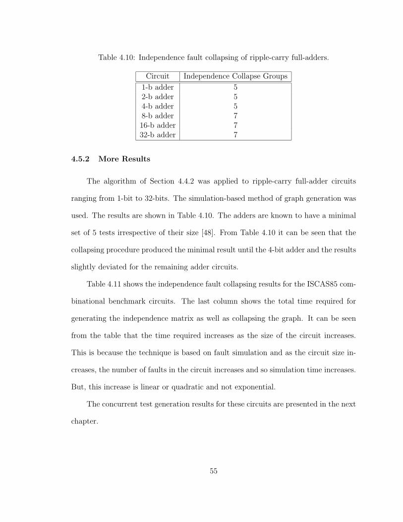
The objective of this work is to find suitable targets for Automatic Test Pattern

Generation (ATPG) such that a minimal test set is obtained for a combinational

circuit. Original concepts of independence fault collapsing and concurrent test gen-

eration are developed and a novel test generation strategy based on these is devised.

Independence fault collapsing groups faults into independent fault subsets such

that each subset includes some faults that cannot be covered by the tests derived for

any other subset. Using these fault subsets, optimally compact tests can be found.

For an equivalence or dominance collapsed fault set an independence graph is gen-

erated using structural and functional independences. Each fault is represented as a

node and an undirected edge between two nodes indicates independence of the corre-

sponding faults; two independent faults cannot be detected by the same test vector. A

“similarity-based” collapsing procedure reduces the graph to a fully-connected graph,

whose nodes specify concurrently-testable fault targets for the ATPG.

v

Given a set of target faults, a concurrent test is an input vector that detects

all (or most) faults in the set. These sets are obtained from the independence fault

collapsing procedure. A new algorithm called the concurrent D algebra is presented

for concurrent test generation.

The independence fault collapsing algorithm and the concurrent D algebra to-

gether produced the minimal set of 12 tests for the 4-bit ALU (74181) circuit. But

due to the complexity involved in generating the independence graph, this technique

was not applied to the ISCAS85 benchmark circuits. A simulation based method was

devised for generating the independence graph and for deriving concurrent tests using

single-fault ATPG.

The simulation based method was applied to the ISCAS85 combinational bench-

mark circuits. The results show that minimal test sets were generated for some

benchmark circuits in CPU times that were almost half of what were required for an

alternative dynamic compaction technique presented in the literature.

vi

Acknowledgments

I would like to gratefully acknowledge the assistance, encouragement, support,

patience and direction provided to me by my advisor, Dr. Vishwani D. Agrawal,

during my stay at Auburn University. It was a great pleasure for me to undergo this

learning experience. I would like to thank Dr. Victor P. Nelson and Dr. Charles E.

Stroud for being on my committee and providing me valuable inputs. I would like to

express my deepest gratitude to my parents and sister whose love and encouragement

is inspiring me to achieve my goals. Finally I would like to thank all my friends here

at Auburn University and also those back in India.

vii

Style manual or journal used LATEX: A Document Preparation System by Leslie

Lamport (together with the style known as “aums”).

Computer software used The document preparation package TEX (specifically

LATEX) together with the departmental style-file aums.sty. The images and plots

were generated using SmartDraw 6 and Microsoft Office Excel 2003.

viii

Table of Contents

List of Tables xi

List of Figures xiii

1 Introduction 11.1 Problem Statement . . . . . . . . . . . . . . . . . . . . . . . . . . . . 11.2 Contribution of Thesis . . . . . . . . . . . . . . . . . . . . . . . . . . 21.3 Organization of Thesis . . . . . . . . . . . . . . . . . . . . . . . . . . 2

2 Background 42.1 Fault Modeling . . . . . . . . . . . . . . . . . . . . . . . . . . . . . . 5

2.1.1 Stuck-at Faults . . . . . . . . . . . . . . . . . . . . . . . . . . 62.2 Fault Collapsing . . . . . . . . . . . . . . . . . . . . . . . . . . . . . . 72.3 Fault Simulation and Test Generation . . . . . . . . . . . . . . . . . . 10

2.3.1 Fault Simulation . . . . . . . . . . . . . . . . . . . . . . . . . 102.3.2 Test Generation . . . . . . . . . . . . . . . . . . . . . . . . . . 11

3 Previous Work on Test Set Minimization 133.1 Static Compaction . . . . . . . . . . . . . . . . . . . . . . . . . . . . 143.2 Dynamic Compaction . . . . . . . . . . . . . . . . . . . . . . . . . . . 163.3 Compaction Based on Independent Faults . . . . . . . . . . . . . . . 183.4 The Berger and Kohavi Method . . . . . . . . . . . . . . . . . . . . . 203.5 Summary . . . . . . . . . . . . . . . . . . . . . . . . . . . . . . . . . 24

4 Independence Fault Collapsing 264.1 Fault Reclassification . . . . . . . . . . . . . . . . . . . . . . . . . . . 264.2 Methods of Finding Independence Relations . . . . . . . . . . . . . . 28

4.2.1 Structural Independence . . . . . . . . . . . . . . . . . . . . . 294.2.2 Implied Independence . . . . . . . . . . . . . . . . . . . . . . 294.2.3 Functional Independence . . . . . . . . . . . . . . . . . . . . . 32

4.3 Independence Graph and Independence Matrix . . . . . . . . . . . . . 334.3.1 Independence Graph . . . . . . . . . . . . . . . . . . . . . . . 334.3.2 Independence Matrix . . . . . . . . . . . . . . . . . . . . . . . 36

4.4 Algorithm for Independence Fault Collapsing . . . . . . . . . . . . . . 364.4.1 Definitions . . . . . . . . . . . . . . . . . . . . . . . . . . . . . 41

ix

4.4.2 Independence Fault Collapsing Algorithm . . . . . . . . . . . 434.4.3 ALU Example . . . . . . . . . . . . . . . . . . . . . . . . . . . 49

4.5 Simulation-Based Independence Fault Collapsing . . . . . . . . . . . . 514.5.1 Algorithm . . . . . . . . . . . . . . . . . . . . . . . . . . . . . 524.5.2 More Results . . . . . . . . . . . . . . . . . . . . . . . . . . . 55

4.6 An Alternative Method for Independence Fault Collapsing . . . . . . 56

5 Concurrent Test Generation 595.1 The Concurrent-D Algebra . . . . . . . . . . . . . . . . . . . . . . . . 61

5.1.1 Four-Bit ALU (74181) . . . . . . . . . . . . . . . . . . . . . . 635.2 Simulation Based Concurrent Test Generation . . . . . . . . . . . . . 64

5.2.1 Algorithm . . . . . . . . . . . . . . . . . . . . . . . . . . . . . 655.2.2 Results . . . . . . . . . . . . . . . . . . . . . . . . . . . . . . . 65

6 Conclusion 716.1 Future Work . . . . . . . . . . . . . . . . . . . . . . . . . . . . . . . . 72

Bibliography 74

Appendices 79

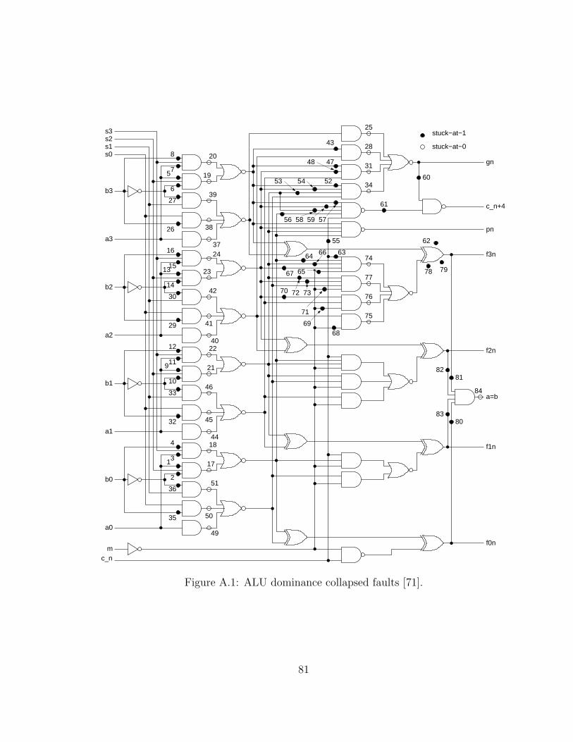
A On the Effectiveness of the Independence Fault Collapsing Al-

gorithm of Subsection 4.4.2 80

B DIMACS Format 84

x

List of Tables

4.1 Independence matrix for c17 benchmark circuit in Figure 4.5. . . . . 37

4.2 Degree of Independence for c17 benchmark circuit of Figure 4.5. . . . 42

4.3 Similarity Metrics for c17 benchmark circuit of Figure 4.5. . . . . . . 43

4.4 Step 1: Computation of degree of independence (DI) for each fault. . 45

4.5 Step 2: Faults ordered according to decreasing degree of independence. 46

4.6 Step 3: Computation of similarity metric for each pair of faults. . . . 47

4.7 Independence fault collapsing of c17 faults. . . . . . . . . . . . . . . . 47

4.8 Independence collapsed fault sets for 4-bit ALU. . . . . . . . . . . . . 51

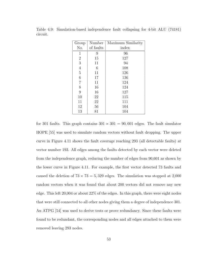
4.9 Simulation-based independence fault collapsing for 4-bit ALU (74181)circuit. . . . . . . . . . . . . . . . . . . . . . . . . . . . . . . . . . . . 53

4.10 Independence fault collapsing of ripple-carry full-adders. . . . . . . . 55

4.11 Independence fault collapsing on ISCAS85 benchmark circuits. . . . . 56

4.12 Results for the c17 circuit. . . . . . . . . . . . . . . . . . . . . . . . . 58

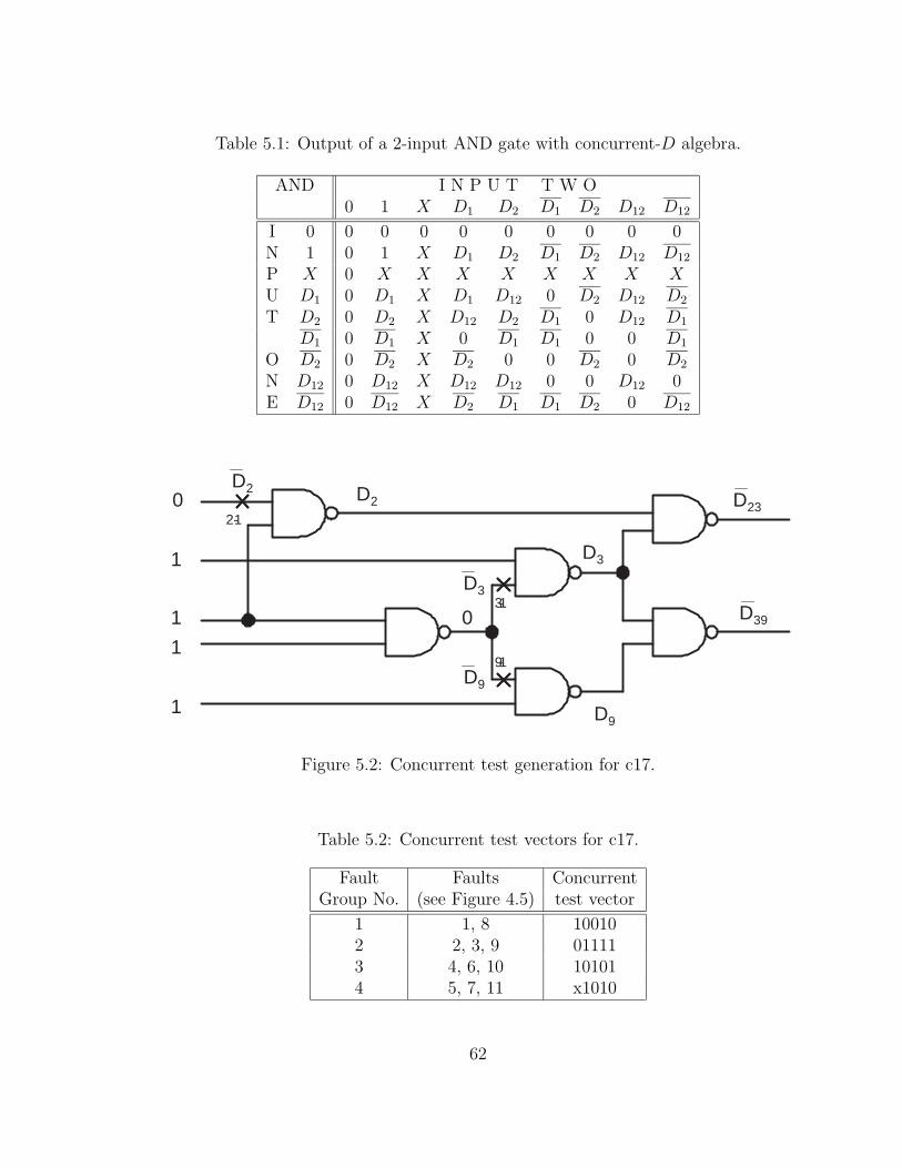
5.1 Output of a 2-input AND gate with concurrent-D algebra. . . . . . . 62

5.2 Concurrent test vectors for c17. . . . . . . . . . . . . . . . . . . . . . 62

5.3 Concurrent test generation for the 4-bit ALU (74181) circuit. . . . . . 63

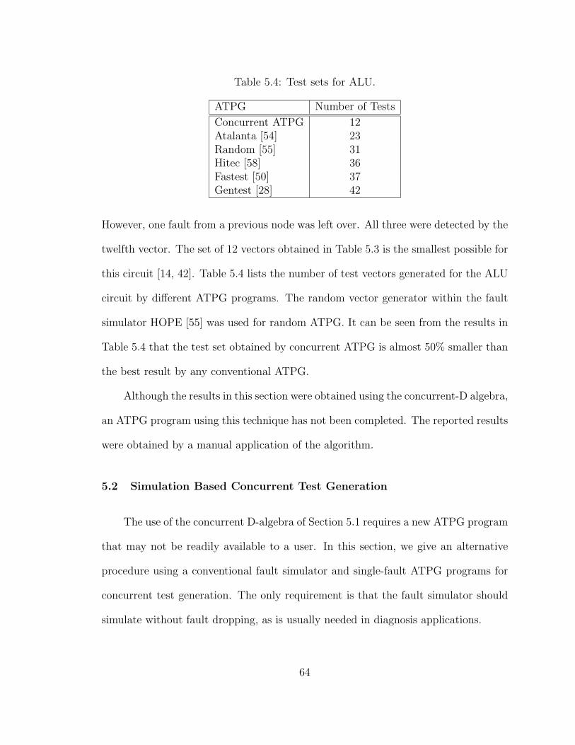
5.4 Test sets for ALU. . . . . . . . . . . . . . . . . . . . . . . . . . . . . 64

5.5 Simulation-based concurrent test generation for the 4-bit ALU (74181)circuit. . . . . . . . . . . . . . . . . . . . . . . . . . . . . . . . . . . . 66

xi

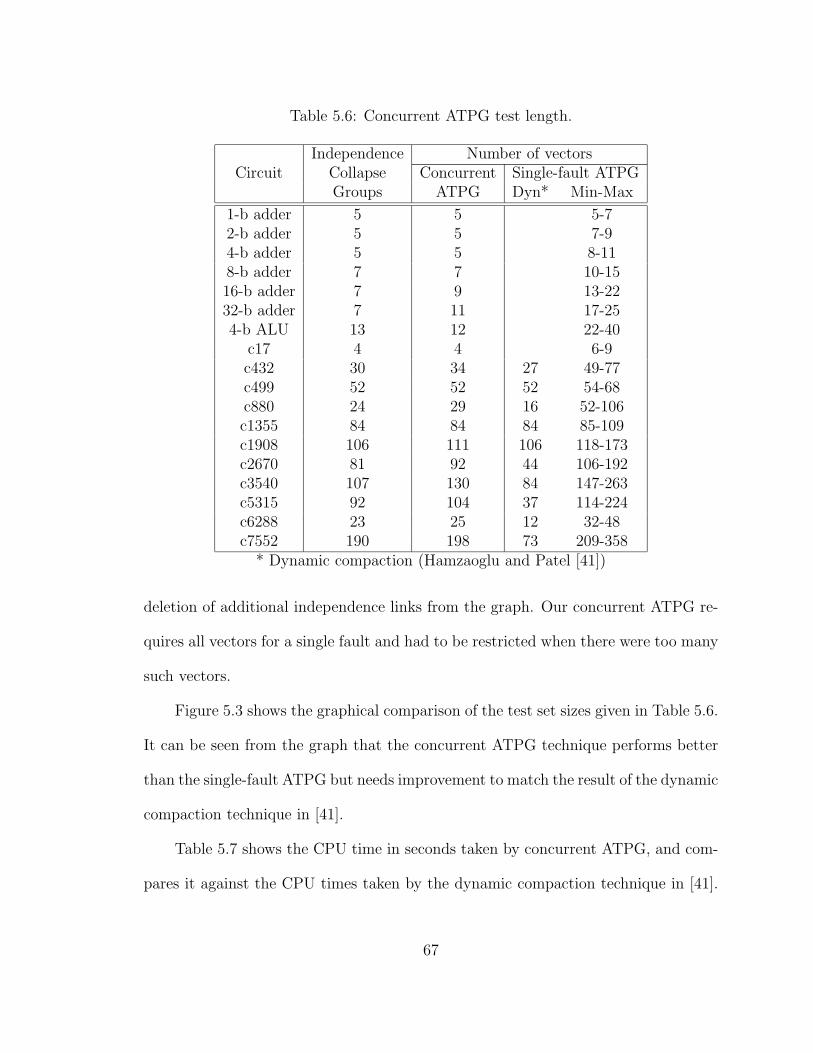
5.6 Concurrent ATPG test length. . . . . . . . . . . . . . . . . . . . . . . 67

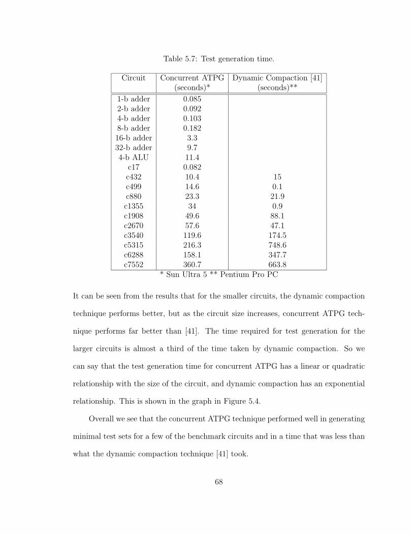
5.7 Test generation time. . . . . . . . . . . . . . . . . . . . . . . . . . . . 68

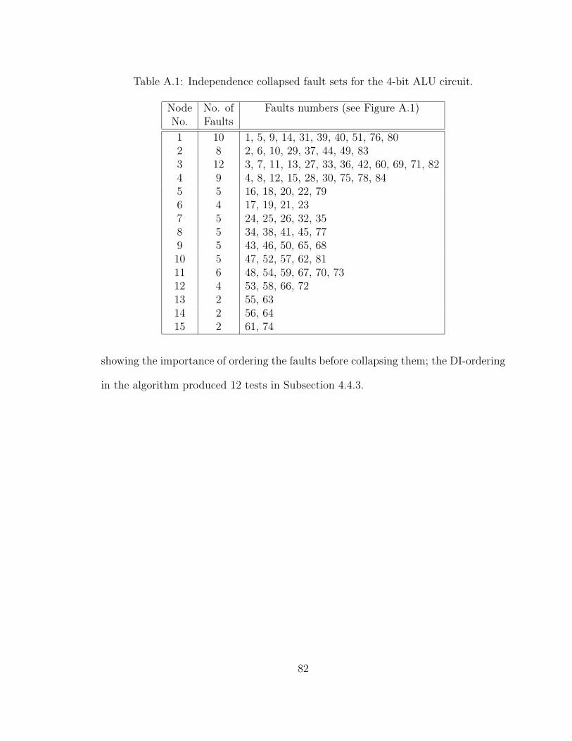
A.1 Independence collapsed fault sets for the 4-bit ALU circuit. . . . . . . 82

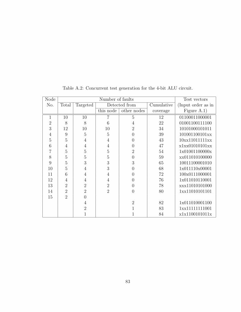
A.2 Concurrent test generation for the 4-bit ALU circuit. . . . . . . . . . 83

xii

List of Figures

2.1 Testing Process. . . . . . . . . . . . . . . . . . . . . . . . . . . . . . . 4

2.2 Fault Collapsing. . . . . . . . . . . . . . . . . . . . . . . . . . . . . . 8

3.1 An example fanout-free circuit. . . . . . . . . . . . . . . . . . . . . . 21

3.2 Characteristic graphs for circuit of Figure 3.1. . . . . . . . . . . . . . 22

3.3 Test generation for circuit of Figure 3.1. . . . . . . . . . . . . . . . . 23

3.4 Problem of finding a minimal test. . . . . . . . . . . . . . . . . . . . . 24

4.1 Test relations of faults F1 and F2 with tests T (F1) and T (F2). . . . 27

4.2 Structural independences of faults of Boolean gates and fanout. . . . 29

4.3 Implied independence between faults of two subnetworks. . . . . . . . 31

4.4 An ATPG-based method for finding all faults that are independent offault Fi. . . . . . . . . . . . . . . . . . . . . . . . . . . . . . . . . . . 34

4.5 Functional dominance collapsed faults [71] of c17 circuit. . . . . . . . 34

4.6 Independence graph for c17 benchmark circuit in Figure 4.5. . . . . . 36

4.7 Largest clique in the independence graph of Figure 4.6. . . . . . . . . 38

4.8 Examples of independence graphs, cliques and collapsed graphs. . . . 40

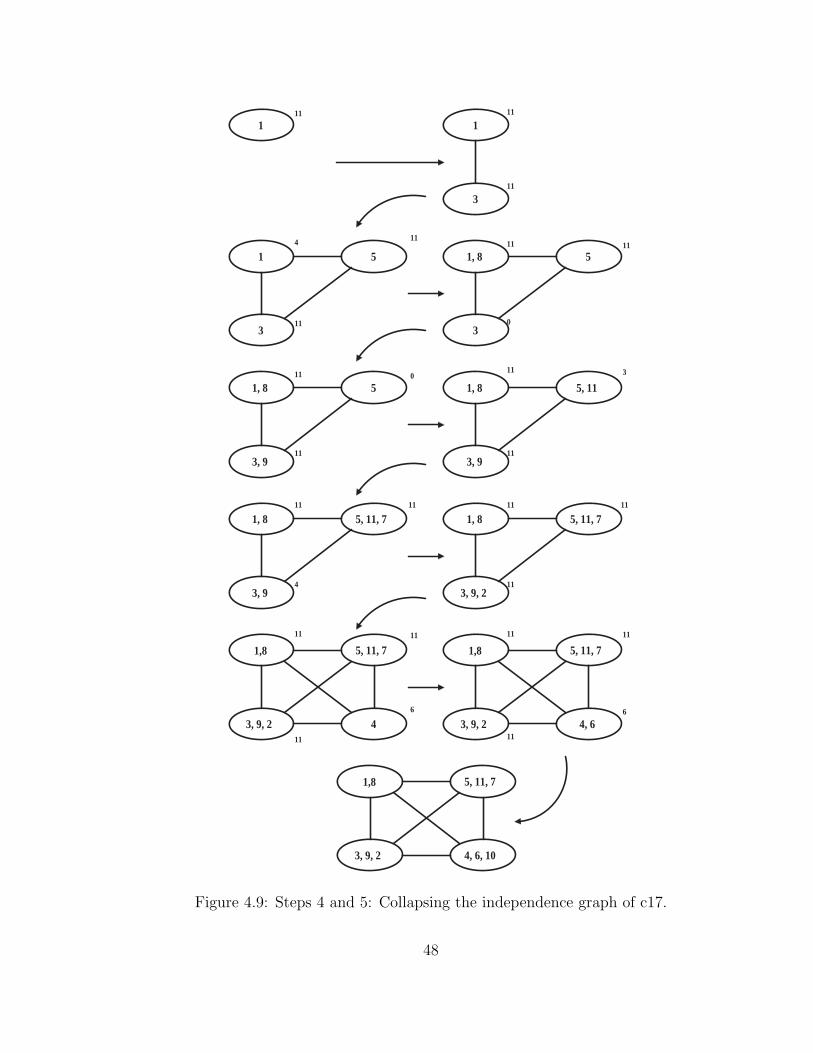
4.9 Steps 4 and 5: Collapsing the independence graph of c17. . . . . . . . 48

4.10 ALU dominance collapsed faults [71]. . . . . . . . . . . . . . . . . . . 50

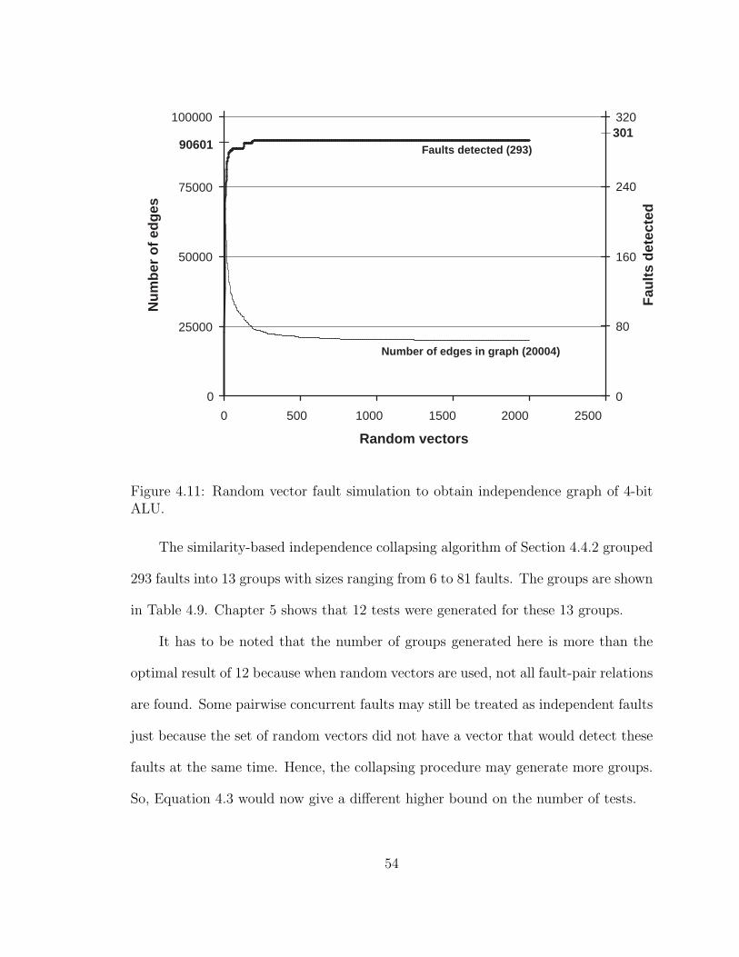
4.11 Random vector fault simulation to obtain independence graph of 4-bitALU. . . . . . . . . . . . . . . . . . . . . . . . . . . . . . . . . . . . . 54

xiii

4.12 Independence collapsing of c17 faults starting from a known clique. . 57

5.1 Generation of concurrent test. . . . . . . . . . . . . . . . . . . . . . . 60

5.2 Concurrent test generation for c17. . . . . . . . . . . . . . . . . . . . 62

5.3 Test set size comparison. . . . . . . . . . . . . . . . . . . . . . . . . . 69

5.4 Test generation time comparison. . . . . . . . . . . . . . . . . . . . . 70

A.1 ALU dominance collapsed faults [71]. . . . . . . . . . . . . . . . . . . 81

xiv

Chapter 1

Introduction

Time is money! This is a phrase that is being put to use by almost everyone

today. Lesser the time spent in doing something, more is the money saved. That

thought is at the back of every test engineer’s mind.

With the advances in science and technology, modern devices are becoming more

complex every day. As the device complexity increases, testing becomes even more

complex. This results in increased test time and higher test cost. At the same

time, the manufacturing cost of a device is going down due to the higher levels of

integration. All this has contributed to a test cost that is an increasing fraction of

the total manufacturing cost. Hence the necessity of reducing the test cost.

To decrease the test cost, the time required to test a device needs to be decreased.

This time can be decreased if the number of tests required to test the device is reduced.

So, we simply need to devise a test set that is small in size. It would be better to

generate a small test set rather than to compact a large test set. This is because the

result of compaction depends on the quality of the original test set. This idea has

motivated the work presented in this thesis.

1.1 Problem Statement

The problem solved in this thesis is: Find a minimal test vector set to detect all

single stuck-at faults in a combinational circuit.

1

1.2 Contribution of Thesis

We have developed a new test generation technique based on independence fault

collapsing and concurrent test generation to produce minimal or near-minimal test

sets for combinational circuits. A novel fault collapsing technique based on indepen-

dent faults groups faults into nodes of a fully-connected graph. The nodes specify

fault targets that are possibly concurrently-testable by an Automatic Test Pattern

Generator (ATPG). The term “concurrently-testable faults,” as defined in this the-

sis, refers to faults that can be tested by a common test. We present new algorithms

for generating concurrent tests. A simulation based approach for complete test gen-

eration, including the independence fault collapsing and concurrent ATPG, is then

presented. Results for benchmark circuits show that the method in fact does generate

minimal test sets for some of the benchmark circuits, but may require improvements

in algorithms and the program implementation for others.

Two papers describing this work have been presented at the Ninth VLSI Design

and Test Symposium (VDAT-2005) and the Fourteenth IEEE Asian Test Symposium

(ATS-2005) and have appeared in the respective proceedings [8, 32].

1.3 Organization of Thesis

The thesis is organized as follows. In Chapter 2, we discuss the basics of testing

and the relevant background on faults and test generation. In Chapter 3, the previ-

ous work on test set compaction is discussed. In Chapter 4, the new independence

fault collapsing algorithm is introduced and results for some benchmark circuits are

presented. Chapter 5 discusses the new concurrent test generation technique with

2

results on benchmark circuits. Conclusions and ideas about future work directions

are discussed in Chapter 6.

3

Chapter 2

Background

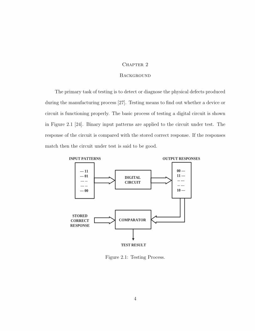
The primary task of testing is to detect or diagnose the physical defects produced

during the manufacturing process [27]. Testing means to find out whether a device or

circuit is functioning properly. The basic process of testing a digital circuit is shown

in Figure 2.1 [24]. Binary input patterns are applied to the circuit under test. The

response of the circuit is compared with the stored correct response. If the responses

match then the circuit under test is said to be good.

DIGITAL CIRCUIT

COMPARATOR

--- 11 --- 01 --- -- --- -- --- 00

00 --- 11 --- -- --- -- --- 10 ---

INPUT PATTERNS OUTPUT RESPONSES

STORED CORRECT RESPONSE

TEST RESULT

Figure 2.1: Testing Process.

4

2.1 Fault Modeling

Physical defects are those that can really occur in a circuit. During chip fabrica-

tion many types of defects can occur, for example, breaks in signal lines, lines shorted

to ground, excessive delays, etc. It might seem that if one wishes to ensure that a

circuit is free from all defects, this could be done by checking that all the functions

of the system are being performed correctly. The problem with this approach is the

complexity of the test needed to completely check out even simple functions. A com-

plete functional test of a simple module with just 65 inputs may take over 1000 years

to complete. On the other hand, if we use information about the structure of the

circuit, we could apply a relatively small number of tests to ensure that a given set

of faults in the circuit did not exist. A representation of a defect at the abstracted

function level is called a modeled fault or simply a fault [24].

In engineering, models bridge the gap between physical reality and mathematical

abstraction [24]. The most important models in testing are those of faults. Fault

modeling is the translation of physical defects to a mathematical construct that can

be operated upon algorithmically and understood by a software simulator for the

purposes of providing a metric for quality measurement [30]. A good fault model

is one that is simple to analyze and yet closely represents the behavior of physical

faults in the circuit. Logical faults represent effects of faults on the behavior of

modeled systems. Physical defects are modeled as logical faults because the analysis

of logical faults is much simpler than the mathematical analysis of physical defects.

Logical fault models can represent many, though not all, physical failures. It is

5

technology-independent and, therefore, technology changes do not affect the methods

for detection of such faults.

2.1.1 Stuck-at Faults

One of the earliest and still widely used fault models is the stuck-at fault. It

is believed that Eldred’s 1959 paper [33] laid the foundation for the stuck-at fault

model, though the paper did not explicitly mention the stuck-at fault. The term

“stuck-at fault” first appeared in the 1961 paper by Galey, Norby and Roth [37]. In

1963, Poage presented a theoretical analysis of stuck-at faults [61].

Stuck-at faults are not only the simplest faults to analyze, but they also have

proved to be very effective in representing the faulty behavior of actual devices. The

simplicity of stuck-at faults is derived from their logical behavior; these faults are

often referred to as logical faults [27].

The stuck-at fault is defined as a fault that forces a fixed value (either 0 or 1)

on a signal line in the circuit, where the signal line can be an input or an output

of a logic gate or flip-flop [24]. So, a stuck-at fault is assumed to affect only the

interconnections between gates. The stuck-at faults are of two types, the stuck-at-1

(s-a-1 or sa1) and stuck-at-0 (s-a-0 or sa0). In general, many stuck-at faults can

be present in a circuit. A circuit with n lines can have 3n − 1 possible stuck line

combinations [24, 27] as each line can be s-a-1 or s-a-0 or fault-free. All combinations

except the one having all lines as fault-free are treated as faults. It is easy to recognize

that even with moderately large values of n, the number of multiple stuck-at faults

will be very large. Therefore, in practice, we only analyze single stuck-at faults. A

circuit with n lines will then have at most 2n single stuck-at faults [24]. The number

6

of faults considered for testing is further reduced by fault collapsing as discussed in

the next section.

2.2 Fault Collapsing

Fault collapsing can be classified into two types; equivalence collapsing and dom-

inance collapsing. Two faults are called equivalent if and only if they transform the

circuit such that the two faulty circuits have identical output functions [24]. Equiv-

alent faults are also called indistinguishable and have exactly the same set of tests.

The set of all faults in a circuit can be partitioned into equivalence sets, such that

all faults in a set are equivalent to each other. The process of selecting one fault

from each equivalence set is called fault collapsing [24]. The fault set thus obtained

is called an equivalence collapsed set.

The relative size of the equivalence collapsed set with respect to the set of all

faults is called the collapse ratio [24]:

Collapse ratio =|Set of collapsed faults|

|Set of all faults|(2.1)

Consider an n-input AND gate. It has a total of 2n + 2 faults. Each of the n + 1

s-a-0 faults on its input and output lines transforms the AND gate to a constant

0 output function. Thus all s-a-0 faults are equivalent. So, equivalence collapsing

reduces the total faults to just n + 2. Similar results are derived for other Boolean

gates as well. It must be noted that faults on a fanout stem and those on the branches

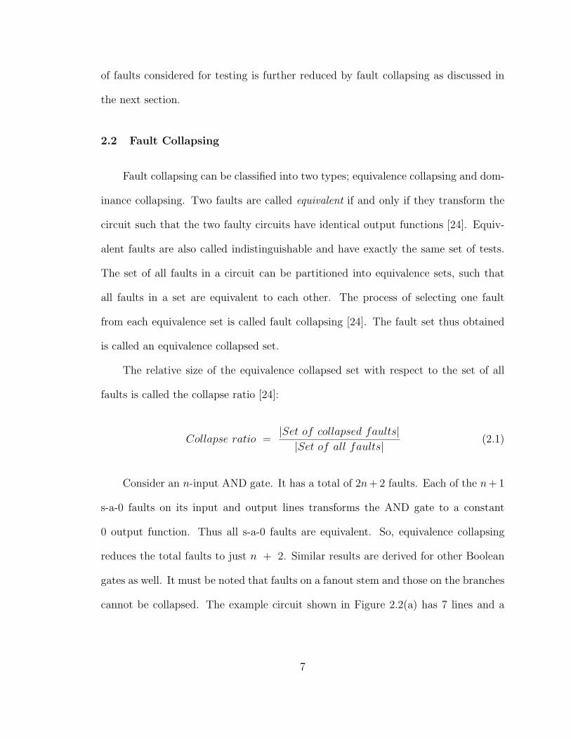
cannot be collapsed. The example circuit shown in Figure 2.2(a) has 7 lines and a

7

(a) Example circuit with all faults.

(b) Equivalence Collapsing.

( c ) Dominance Collapsing.

sa0 sa1

sa0 sa1

sa0 sa1

sa0 sa1

sa0 sa1

sa0 sa1

sa0 sa1

sa0 sa1

sa1

sa0 sa1

sa1 sa1

sa0

sa0 sa1

sa1

sa0 sa1

sa1

Figure 2.2: Fault Collapsing.

8

total of 14 faults. Figure 2.2(b) shows the faults after equivalence collapsing. The

number of faults is reduced to just 8. So the collapse ratio is 8/14 = 0.57.

In equivalence fault collapsing we only collapse the faults that are indistinguish-

able. If we are prepared to give up on the diagnostic resolution, i.e., the ability to

distinguish between faults, more collapsing is possible. This is accomplished by using

the concept of fault dominance. In large circuits, where coverage (detection) of faults

rather than their exact location (diagnosis) is a more important, dominance fault

collapsing may be desirable.

Consider two faults F1 and F2. If all tests of fault F1 detect another fault

F2, then F2 is said to dominate F1. The two faults are also called “conditionally

equivalent” with respect to the test set of F1 [24]. When two faults F1 and F2

dominate each other, they are then equivalent. So, dominance is a more basic relation

than equivalence.

Consider the n-input AND gate again. For the AND gate, the output stuck-at 1

fault dominates all the input s-a-1 faults. So, after dominance collapsing, the fault set

reduces to n+1. For the example circuit of Figure 2.2, dominance collapsing reduces

the number of faults to just 6 as shown in Figure 2.2(c). So, the collapse ratio now

becomes 6/14 = 0.43. Dominance collapsing always results in a smaller test set than

the equivalence collapsed set.

A “dominated” fault can become redundant due to the circuit structure. A fault

that does not modify the input-output function of the circuit and cannot be detected

by any test is called a redundant fault. If a dominated fault is redundant, no test would

be obtained for the dominating fault even though that may be detectable. Though

dominance collapsing produces a smaller collapsed fault set, the tests for the collapsed

9

faults may not guarantee a 100% fault coverage. Hence equivalence collapsing is more

popular. The size of the fault set can be further reduced by performing functional

collapsing. The faults in a hierarchical circuit can be collapsed using hierarchical fault

collapsing [9, 10, 66, 70, 72].

Most definitions for fault equivalence and dominance, appearing in the literature,

correspond to single output circuits. For such circuits, fault equivalence defined on

the basis of indistinguishability (identical faulty functions) implies that the equivalent

faults have identical tests. However, for multiple output circuits, two faults that

have identical tests can be distinguishable. This leads to expanded definitions for

equivalence and dominance [70, 72].

2.3 Fault Simulation and Test Generation

2.3.1 Fault Simulation

A logic simulator or true-value simulator computes the response of a given fault-

free circuit for given input stimuli. A fault simulator determines the coverage of a

given set of faults by a given set of input vectors through simulation of the circuit.

The fault simulator indicates which faults are detected by each input vector.

There are several methods of fault simulation, the simplest being the serial fault

simulation. In this method, a single fault is introduced into the circuit model and

simulation is run like true-value simulation. The circuit response is compared with

the stored response of the fault-free circuit. As soon as the fault is detected, the

simulation is stopped and a new simulation is started for another fault. This fault

simulation method, though simple, is very time consuming.

10

Another technique of fault simulation, which simulates more than one fault in

one pass is called parallel fault simulation. The idea of parallel fault simulation is to

use the bit-parallelism of logical operations in a digital computer [24]. The parallel

fault simulator can simulate a maximum of w − 1 faults in one pass, where w is the

machine word size. So, a parallel fault simulator may run w − 1 times faster than a

serial fault simulator. If fault dropping is used, the fault simulator will gain speed.

The act of dropping a fault from the fault list as soon as it is detected is called fault

dropping.

Other fault simulation algorithms include deductive [15], concurrent [75, 76],

TEST-DETECT [69], differential [29], etc.

2.3.2 Test Generation

Test generation approaches can be classified into three categories: exhaustive,

random and deterministic. If the number of inputs for a combinational circuit is

small, exhaustive tests consisting of all possible input vectors to ensure 100% fault

coverage can be used. Random test generation is a simple and low-cost method in

which input vectors are generated randomly. A vector is retained only if new faults

are detected by that vector. But, the number of random vectors needed for high

fault coverages can be extremely large. So, random vectors are used in conjunction

with deterministic vectors [5]. Random vectors are used for achieving an initial 60-

80% fault coverage. Then, tests are generated for the remaining faults by using

deterministic methods.

We restrict our discussion to combinational circuits. In order for a fault to be

detected, the fault must be first activated by a test vector, and then its result must

11

be propagated to a primary output by the same vector. A test vector t activates a

fault, when it generates an error by creating different values for faulty and fault free

circuits at the site of the fault. The vector t propagates the error to a primary output

w, when at least one path between the fault site and the output w has different value

for faulty and fault free circuits. A line in the faulty circuit, whose value differs from

that in the fault free circuit when subjected to the vector t is said to be sensitized for

the fault f . The path composed of sensitized lines is called a sensitized path.

Deterministic test pattern generation produces tests by processing a model of the

circuit. It uses the notion of activation of the fault, and then the propagation of the

faulty result through a sensitized path to a primary output. This is more expensive

in terms of computational effort than the random method, but the resulting tests

are often shorter and have higher coverage. Therefore, the cost of test application

is much reduced relative to that of random testing. In deterministic test generation,

the search for a solution involves a decision process for selecting an input vector from

the set of partial solutions using an algorithmic procedure known as backtracking.

In backtracking, all previously assigned signal values are recorded, so that the search

process is able to avoid those signal assignment that are inconsistent with the test

requirement. The exhaustive nature of the search causes the worst-case complexity

to be exponential in the number of signals in the circuit [36, 44]. To minimize the

total time, a typical test generation program is allowed to do only a limited search in

the number of trials or backtracks, or the CPU time.

The most widely used automatic deterministic test pattern generation algo-

rithms are: D-algorithm [68], PODEM (Path-Oriented Decision Making) [38] and

FAN (Fanout-Oriented Test Generator) [35].

12

Chapter 3

Previous Work on Test Set Minimization

Early research on test generation was directed toward efficiently generating a

complete test set for a given circuit [35, 38, 68]. Once that objective was met, the

next target was to generate smaller test sets. In the past two decades a lot of work

has been done in the area of test set minimization. This work continues since the

problem of generating a minimum size test set for a combinational circuit is NP-

Hard [52]. Every new technique developed performs a little better than the previous

one and hence motivates one to go even further as there is still hope of reaching the

lower bound or just to close the gap further.

By reducing the test sequence length, the memory requirements during test ap-

plication and the test application time are reduced. The extent of test compaction

possible for deterministic test sequences indicates that test pattern generators spend

a significant amount of time generating test vectors that are not necessary. So, al-

gorithms for finding compact test sequences remains an open problem in the area of

efficient deterministic Automatic Test Pattern Generation (ATPG).

Various techniques have been proposed for test set compaction, some of which

are discussed in the following sections. These techniques have been grouped into

categories depending on the type of compaction used.

13

3.1 Static Compaction

Static compaction [1] is performed after the test set has been generated and

is independent of the test generation process, so it has been referred to as post-

generation compaction [26]. Several static compaction algorithms based on different

heuristics exist in the literature and are discussed next.

One technique of static compaction eliminates the redundant test vectors from

the test set. A redundant test vector is a vector such that each fault detected by

that vector is also detectable by some other vector in the test set. Most combina-

tional ATPG methods use Random Pattern Generators (RPG) [3, 4] to obtain about

60% fault coverage [24], and then use an ATPG algorithm to generate tests for the

remaining faults. This process can be one of the main sources of redundant test vec-

tors. Redundant test vectors can be identified using set covering [21] or test vector

reordering with fault simulation [64]. Another technique for removing the redendant

vectors is reverse order fault simulation [73]. This technique is used in many test

generation procedures to drop tests that detect faults that are also detected by tests

generated later in the test generation procedure.

A more sophisticated static compaction method is described by Goel and Ros-

ales [39], where pairs of compatible test vectors, that do not conflict in their specified

(0, 1) values, are repeatedly merged into single vectors. This method is suitable only

for patterns generated by an ATPG program, where the unassigned inputs are left as

don’t care (X). An example of this technique is given below [24]:

Consider the following test set:

t1 = 01X t2 = 0X1 t3 = 0X0 t4 = X01

14

By first combining t1 and t3, and then t2 and t4, we obtain the compacted test set:

t13 = 010 t24 = 001

When two compatible tests ta and tb are combined into one test tab, the detected

faults will be the union of faults detected by ta and tb. Also, the compacted test set

will vary depending on the order in which vectors are compacted.

The influence of the order in which vectors are merged can be eliminated by using

the integer linear programming (ILP) method [34, 43, 56]. ILP guarantees to find the

minimal test set contained in the given vector set. Thus, the absolute minimality can

be only expected if one starts with an exhaustive vector set. The ILP method has

also been used to minimize the N -detection test sets [49], where each fault is detected

by at least N different vectors in the set. The derivation of such tests is motivated

by the observation that vector sets with N ≈ 5 have a higher coverage of real defects

than the conventional single-detection test sets. One should, however, remember that

the complexity of the ILP solution is exponential.

Static compaction can be helpful in some situations because it does not require

any modifications to the test generation procedure. Though static compaction adds

to the test generation time, this time is usually small compared to the total test gen-

eration time. But optimal static compaction algorithms are impractical, so heuristic

algorithms are used. During static compaction, since the patterns in the given set

are not modified or are only passively modified, i.e., only unspecified bits in patterns

are modified, it achieves little reduction for a highly incompatible test set. Static

compaction could still be useful after dynamic compaction is used, to further reduce

15

the length of the test sequence. The dynamic compaction techniques are discussed in

the next section.

3.2 Dynamic Compaction

Dynamic compaction [39] is a process that is integrated into the test generation

process, generally attempting to generate vectors such that each detects a large num-

ber of faults. So the fault coverage of each vector is maximized during test generation

to reduce the total number of test vectors. In dynamic compaction, a currently gen-

erated vector is used as constraints at primary inputs, and the next target fault is

carefully selected such that a test pattern can be generated under the constraints [26].

One of the very first dynamic compaction techniques was presented by Goel

and Rosales [39]. Here, every partially-complete vector from ATPG is processed

immediately after it is generated, by assigning 0 or 1 to primary inputs with don’t

care (X) values to enhance the vector to detect additional faults. Another dynamic

compaction method [40] analyzes the internal circuit values produced by a partially-

specified vector and selects a secondary target fault for which ATPG is more likely

to succeed.

An alternative approach to test compaction reduces the test set size by pruning

the essential faults of some test vectors to make them redundant. A test vector

becomes redundant if it detects no essential faults. A fault is essential if it is detected

only by a single test vector [26, 45]. Compaction methods based on essential fault

pruning have been classified in the literature as static techniques as they are applied

after the test generation process. But, we will consider them as dynamic techniques

as the test vectors are modified during the process. Algorithms based on essential

16

fault pruning fall into two categories. In the first category, the essential faults of the

test vector to be eliminated are pruned by modifying other test vectors in the test

set in such a way that they detect their already detected faults in addition to the

pruned essential faults. Several algorithms presented in the literature [26, 67] belong

to this category. On the other hand, in the second category, a set of N test vectors

is replaced by a set of M < N new test vectors. The basic idea is to determine the

faults that are detected only by one or more test vectors among the N test vectors to

be replaced, and find M < N test vectors that detect all those faults. The algorithms

presented by Kajihara et al. [46] belong to the second category.

Another dynamic compaction technique is called double detection [45, 47]. This

technique maximizes the number of faults that a new test vector detects out of the

yet-undetected faults as well as out of the already-detected ones. Thus, it reduces

the number of tests and allow tests generated earlier in the test generation process

to be dropped. This technique also incorporates a static compaction technique called

two by one which simply selects two vectors and replaces them by a single one, without

loss of fault coverage.

Dynamic compaction has also been done using fault simulation by the criti-

cal path tracing algorithm to select a secondary target fault already activated by a

partially-specified test vector [2]. A test generation technique, known as the sub-

scripted D-algorithm [19], uses multiple path sensitization to derive a test for a given

fault target such that a large number of other faults is also detected.

A recent dynamic compaction technique [41] makes use of two algorithms called

redundant vector elimination and essential fault reduction for generating compact test

sets for combinational circuits. These algorithms along with dynamic compaction [39]

17

and a heuristic for estimating the lower bound are incorporated into an advanced

ATPG system for combinational circuits called MinTest. The results [41] are better

than any others published for the ISCAS85 [23] and ISCAS89 [22] benchmark circuits.

But, this technique is computationally expensive.

Though dynamic compaction produces smaller test sets (It has been experimen-

tally shown that for large combinational circuits, dynamic compaction can reduce

the test set by 50% [16]), most dynamic compaction techniques are computationally

expensive. Dynamic compaction techniques based on indpendent faults are discussed

in the next section.

3.3 Compaction Based on Independent Faults

Compaction techniques based on independent faults fall under the dynamic com-

paction category. But since our focus is on independent faults, we will discuss these

techniques in a separate section. Two faults are said to be independent faults if and

only if they cannot be detected by the same test vector [13, 14].

Akers and Krishnamurthy were the first to present test generation and com-

paction techniques based on independent faults [13]. They define an independent

fault set as one in which no two faults can be detected by the same test. The inde-

pendent faults are good target faults for test generation, as the minimum test set size

cannot be smaller than the size of the largest set of independent faults. Thus, the

tests for independent faults can be considered necessary. Since finding a maximum

independent fault set is a difficult problem, heuristics have to be used.

Once a maximal set of independent faults is computed, tests are generated for

that fault set. This process is repeated for a different maximal set of independent

18

faults. An attempt is then made to merge the two vector sets into a single set, smaller

than the union of the two sets. Unspecified values are used for this purpose. This

procedure is repeated for other maximal sets of independent faults, until all faults

are detected [13]. Results for benchmark circuits are not given. Also a fault matching

procedure was used to find sets of compatible faults, i.e., faults that can be detected

by a single test vector, from the independent fault sets. However, these fault sets

were not used to generate minimal test sets. It has been proved [74] that many of

the compatible fault sets published earlier [13] could not be covered by a single test

vector. Though this technique did not provide the best results, it became the basis

for later work on independent faults.

A compaction technique based on independent faults is COMPACTEST [63].

Here, maximal compaction, which is an enhancement to dynamic compaction, is pro-

posed to assign as many don’t care bits as possible in a test vector before aiming at

the next target fault. To further increase the fault coverage of a generated pattern, a

backtrace procedure called rotating backtrace is developed to activate as many sensi-

tized paths as possible during test generation for detection of additional undetected

faults. In addition to the above considerations, the compaction results are also af-

fected by the order of target faults. The concept of compatible fault set [13] is applied

to determine the order of target faults. COMPACTEST achieved improvements of

up to 10 times over previously known test set sizes using simple and fast heuristics.

Another technique based on independent faults, as presented by Tromp [74], is a

modification of the original technique [13]. In this, the independent fault set procedure

is improved to derive larger independent fault sets and to get a better estimate of

the lower bound on the minimum test set size. The implication procedure was also

19

improved. The results presented for the ISCAS85 benchmark circuits showed that

the technique was able to generate tests only for the smaller benchmark circuits and

those results too were far from being optimal.

An algorithm referred to as independent fault clustering is based on the concept

of test vector decomposition [59]. Also, one of the compaction techniques discussed in

the previous section also makes use of independent fault sets [41].

3.4 The Berger and Kohavi Method

In 1973, Berger and Kohavi presented a method for generating the minimum size

test set for a fanout-free combinational circuit [20]. This method is discussed here

because in the initial stages of the research presented in this thesis, we attempted to

extend this method for any combinational circuit. But, despite our efforts, we were

not able to do so. The method is discussed briefly with an example in the following

paragraphs.

We partition the test set T into two disjoint subsets T1 and T0 where T1 consists

of all tests for which the circuit response is 1 and T0 consists of all tests for which

the circuit response is 0. Also, R1 consists of all faults covered by T1 and R0 consists

of all faults covered by T0. These two subsets are disjoint for a circuit that is free

from fanouts. Besides, this circuit has only a single primary output. The union of

any minimal subset of T0 covering R0 and any minimal subset of T1 covering R1

constitutes a minimal test set for the given circuit.

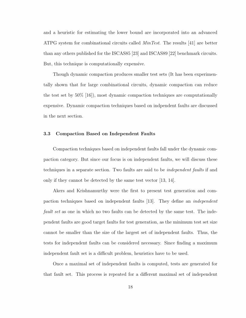
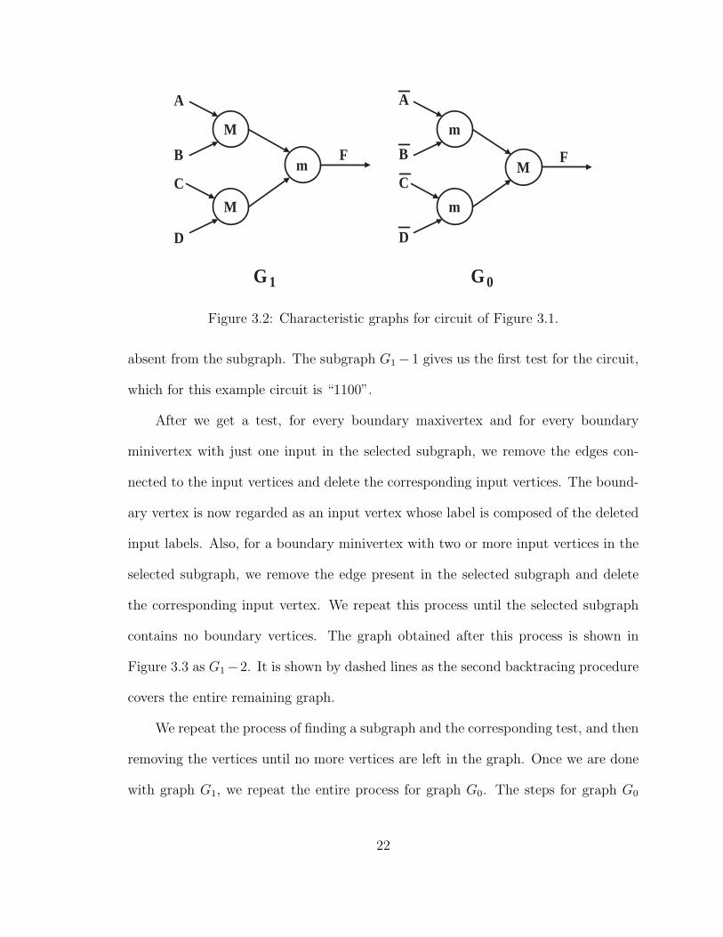
The network structure is represented by two characteristic graphs denoted by G1

and G0 where G1 represents the network when its output is 1 and G0 represents the

network when its output is 0. The gates in the network are represented in the graphs

20

A

B

C

D

F

Figure 3.1: An example fanout-free circuit.

as maxivertices and minivertices. A gate is represented by a maxivertex (M) when

for its output to be sensitized all its inputs must be sensitized. A gate is represented

by a minivertex (m) when for its output to be sensitized only one of its inputs needs

to be sensitized. For example, the AND-gate will be a maxivertex in G1 while it will

be a minivertex in G0. A simple fanout-free circuit is shown in Figure 3.1. Figure 3.2

shows the characteristic graphs for the circuit of Figure 3.1.

The test generation procedure for the circuit in Figure 3.1 is shown in Figure 3.3.

First consider the characteristic graph G1. In this graph, we start tracing back from

the output and choose a subgraph such that during the backtracing when we reach

a minivertex, we continue through exactly one of its inputs, and when we reach a

maxivertex, we continue through all its inputs. We follow this backtracing until we

reach primary inputs. Thus, backtracing traverses a subgraph. One such subgraph

is shown by dashed lines in Figure 3.3 as G1 − 1. For the subgraph, we assign a 1 to

the primary inputs present in the subgraph and a 0 to the remaining inputs that are

21

M

M

m

m

m

M

A

B

C

D

A

B

C

D

F F

G 1 G 0

Figure 3.2: Characteristic graphs for circuit of Figure 3.1.

absent from the subgraph. The subgraph G1 − 1 gives us the first test for the circuit,

which for this example circuit is “1100”.

After we get a test, for every boundary maxivertex and for every boundary

minivertex with just one input in the selected subgraph, we remove the edges con-

nected to the input vertices and delete the corresponding input vertices. The bound-

ary vertex is now regarded as an input vertex whose label is composed of the deleted

input labels. Also, for a boundary minivertex with two or more input vertices in the

selected subgraph, we remove the edge present in the selected subgraph and delete

the corresponding input vertex. We repeat this process until the selected subgraph

contains no boundary vertices. The graph obtained after this process is shown in

Figure 3.3 as G1−2. It is shown by dashed lines as the second backtracing procedure

covers the entire remaining graph.

We repeat the process of finding a subgraph and the corresponding test, and then

removing the vertices until no more vertices are left in the graph. Once we are done

with graph G1, we repeat the entire process for graph G0. The steps for graph G0

22

G 1 -1

G 0 -1

G 1 -2

G 0 -2

M

M

m

A

B

C

D

F

M

m C

D

F

m

m

M

A

C

F

m

m

M

A

B

C

D

F

1100 0011

1010 0101

Figure 3.3: Test generation for circuit of Figure 3.1.

are shown in Figure 3.3 as G0 − 1 and G0 − 2. The tests obtained during this entire

process on graphs G1 and G0 give us a minimal test set. For the example circuit of

Figure 3.1, the minimal test set consists of 4 test vectors, 1100, 0011, 1010 and 0101.

This work was later extended [62] for a small class of combinational circuits

with nonreconvergent fanouts, but the work could not be extended for all classes of

combinational circuits. Considering the complexity of such procedures, we note that

the minimum test set problem for a very small class of combinational circuits may

23

T ( F1 ) T ( F2 )

v 1 v 2 v 3

Test set for fault F1

Test set for fault F2

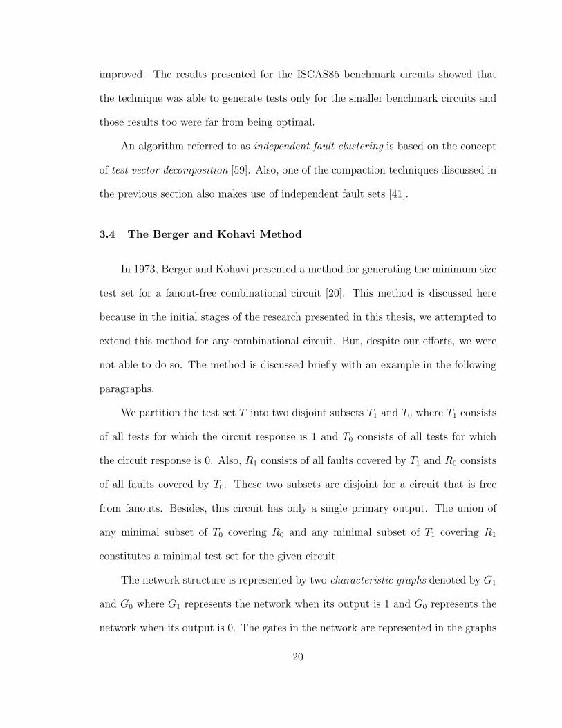
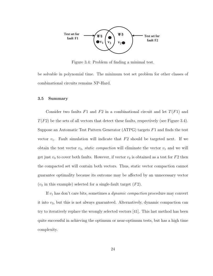
Figure 3.4: Problem of finding a minimal test.

be solvable in polynomial time. The minimum test set problem for other classes of

combinational circuits remains NP-Hard.

3.5 Summary

Consider two faults F1 and F2 in a combinational circuit and let T (F1) and

T (F2) be the sets of all vectors that detect these faults, respectively (see Figure 3.4).

Suppose an Automatic Test Pattern Generator (ATPG) targets F1 and finds the test

vector v1. Fault simulation will indicate that F2 should be targeted next. If we

obtain the test vector v3, static compaction will eliminate the vector v1 and we will

get just v3 to cover both faults. However, if vector v2 is obtained as a test for F2 then

the compacted set will contain both vectors. Thus, static vector compaction cannot

guarantee optimality because its outcome may be affected by an unnecessary vector

(v2 in this example) selected for a single-fault target (F2).

If v1 has don’t care bits, sometimes a dynamic compaction procedure may convert

it into v3, but this is not always guaranteed. Alternatively, dynamic compaction can

try to iteratively replace the wrongly selected vectors [41]. This last method has been

quite successful in achieving the optimum or near-optimum tests, but has a high time

complexity.

24

Figure 3.4 shows a shortcoming of the single-fault ATPG algorithm, which must

be overcome by compaction. The required test, v3, would have been found if we

targeted both faults F1 and F2 together and sought a common test. These problems

of (1) identifying suitable target fault sets and (2) concurrent test vector generation

are discussed in the following chapters. Although, test generation for multiple target

faults has been addressed in the literature [26, 27, 47], the algorithms and applications

presented next are novel.

25

Chapter 4

Independence Fault Collapsing

In this chapter, we will present a new algorithm for collapsing (grouping) faults

into fault subsets such that all or most faults in each subset will have a single test.

Steps required prior to applying the collapsing algorithm are also discussed here. The

ideas and analyses given in this chapter have appeared in recent papers [8, 32].

4.1 Fault Reclassification

Consider two faults F1 and F2 with test sets T (F1) and T (F2), respectively.

Four possible test relations can exist between the two faults. These are shown in

Figure 4.1. The first two relations of equivalence and dominance [24] are commonly

used for fault collapsing to reduce the number of faults to be targeted during ATPG.

When two faults have the exact same test set, they are said to be equivalent

faults. In such a situation, only one fault is targeted, as its detection guarantees the

detection of the other fault. So, the size of the target fault list is reduced. Dominance

collapsing further reduces the size of the target fault list. In an equivalence collapsed

fault list when two faults F1 and F2 satisfy the relation T (F1) ⊃ T (F2), meaning

F1 dominates F2, fault F1 is dropped from the target fault set.

An equivalence collapsed fault set always, and a dominance collapsed set mostly,

generates tests covering all faults. But, the number of test vectors generated is

often significantly larger than the minimum number required. The reason for this

26

T(F2)

(a) F1 and F2 are equivalent. (b) F1 dominates F2.

T(F1) T(F1) T(F2)

(c) F1 and F2 are independent.

T(F2)

(d) F1 and F2 are concurrently testable.

T(F1)=T(F2)

T(F1)

Figure 4.1: Test relations of faults F1 and F2 with tests T (F1) and T (F2).

is explained by Figures 4.1 (c) and (d). Two faults, F1 and F2, in the collapsed set

can be either independent [13, 14], i.e., they have no common test, or concurrently-

testable, i.e., they have common tests. In the absence of any knowledge of these

behaviors, we target both faults. If they are independent then we get two tests,

which are essential. If they are concurrently testable then we may get one vector (if

we were lucky) or two vectors, although only one would have been sufficient. Thus,

independence and concurrently-testable properties of faults may be used to improve

the efficiency of tests. We make the following observations:

• If two faults are independent, then no concurrent test is possible for them. A

trivial case consists of two faults (with opposite polarity) of the same line.

• If two faults are equivalent, then any test for either fault is a concurrent test

for both.

27

• If one fault dominates the other fault, then any test for the dominated fault is

a concurrent test for both faults.

• Two faults having neither a concurrent test nor an exclusive test [6], are both

redundant.

From the above observations we have the definitions for independent faults and

concurrently-testable faults:

Definition 1: Two faults are independent if and only if they cannot be detected

by the same test vector [13, 14].

Definition 2: Two faults that neither have a dominance relationship nor are

independent are defined as concurrently-testable faults.

A pair of concurrently-testable faults has two types of tests:

1. Each fault has an exclusive test that does not detect the other fault [6].

2. A common test that detects both faults. We define this as a concurrent test.

Concurrently-testable faults have also been referred to as compatible faults in the

literature [13].

4.2 Methods of Finding Independence Relations

Independent faults and concurrently-testable faults were defined in Section 4.1.

Now, given a pair of faults, we need to find the relation that exists between them,

i.e., whether they are independent of each other or they are concurrently-testable.

(A dominance collapsed fault list is assumed.) We provide three methods for finding

these relations as discussed in the following subsections.

28

sa0 sa1sa0

sa1

sa1 sa0

sa0

sa1

sa1sa1

sa1

sa0

sa0

sa0 sa0

sa1

sa0 sa1

sa0 sa1

Figure 4.2: Structural independences of faults of Boolean gates and fanout.

4.2.1 Structural Independence

Structural independences of faults of Boolean gates can be easily found and are

shown in Figure 4.2. Here the faults shown are after equivalence and dominance fault

collapsing. This is because the faults with equivalence or dominance relations cannot

be independent. As an example, consider a 2-input AND gate. After dominance

collapsing, the three faults in the target fault list are stuck-at-1 faults on each of

the two inputs and a stuck-at-0 fault on the output. No pair of these faults has a

common test and hence all three faults are independent of each other. The mutual

independence of a pair of faults is shown by a two-sided arrow in Figure 4.2, which

also shows the independence relations for other Boolean gates and a fanout.

4.2.2 Implied Independence

Using the results of Section 4.2.1, many other independences can be determined:

29

1. Implication of equivalence: If two faults are equivalent then all faults that are

independent of one fault are also independent of the other fault.

2. Implication of dominance: If one fault dominates a second fault then all faults

that are independent of the first fault are also independent of the second fault.

The proofs for the above statements can be easily given and so are eliminated here.

The implied fault independences can be determined in a hierarchically described

circuit. This technique would be based on hierarchical fault collapsing [9, 10, 66,

70, 72]. In hierarchical fault collapsing, faults are collapsed within small subcircuits

and the collapsed fault sets are saved in libraries. The collapse data is stored in the

form of a dominance graph, which contains pair-wise dominance relations among the

collapsed fault set and the input and output faults of the subcircuit. The latter are

included to determine equivalences between faults of two or more subnetworks when

they are connected together. Similar to dominances and equivalences, independence

relations remain valid through hierarchy.

Theorem 1: If two faults inside a subnetwork are independent then they remain

independent when the subnetwork is embedded in a larger combinational circuit.

Proof: Consider two faults F1 and F2 of a combinational subnetwork, such that

they are independent. First, consider the detection of these faults in the stand alone

subnetwork. We apply vectors directly to the inputs of the subnetwork and observe

its outputs for fault detection. Let v1 be the test set for fault F1 and v2 be the test

set for fault F2 in the stand alone subnetwork. When this subnetwork is embedded

in a larger combinational circuit, the inputs of the subnetwork will become internal

lines in the larger circuit. A valid test for fault F1 is then a primary input vector that

30

ind.

F4F1 F2 F3

F7 F8

ind. equ.

implied independence

implied independence

F6F5

subnetwork Bsubnetwork A

dom.

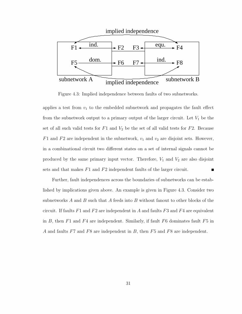
Figure 4.3: Implied independence between faults of two subnetworks.

applies a test from v1 to the embedded subnetwork and propagates the fault effect

from the subnetwork output to a primary output of the larger circuit. Let V1 be the

set of all such valid tests for F1 and V2 be the set of all valid tests for F2. Because

F1 and F2 are independent in the subnetwork, v1 and v2 are disjoint sets. However,

in a combinational circuit two different states on a set of internal signals cannot be

produced by the same primary input vector. Therefore, V1 and V2 are also disjoint

sets and that makes F1 and F2 independent faults of the larger circuit.

Further, fault independences across the boundaries of subnetworks can be estab-

lished by implications given above. An example is given in Figure 4.3. Consider two

subnetworks A and B such that A feeds into B without fanout to other blocks of the

circuit. If faults F1 and F2 are independent in A and faults F3 and F4 are equivalent

in B, then F1 and F4 are independent. Similarly, if fault F6 dominates fault F5 in

A and faults F7 and F8 are independent in B, then F5 and F8 are independent.

31

4.2.3 Functional Independence

In a large circuit, not all independences can be derived by structural analysis.

The most general independence relations are functional and we give a procedure to

find them. Consider a single-output combinational circuit with output function C0

and two single stuck-at faults, Fi and Fj. We denote the faulty functions as Ci and

Cj, respectively. For Fi and Fj to be independent, the following equation must be

satisfied for all inputs:

(C0 ⊕ Ci).(C0 ⊕ Cj) = 0 (4.1)

Each clause in this equation is the test condition for a fault. Only for a test input

the clause becomes true. The equation means that no input vector can make both

clauses true, simultaneously. Equation 4.1 can be written as,

(C0 ⊕ Ci)C0 ⊕ (C0 ⊕ Ci)Cj = 0 (4.2)

Equation 4.2 shows that if we construct a circuit (C0⊕Ci)C0, then a faulty circuit

(C0 ⊕ Ci)Cj will be indistinguishable when Fi and Fj are independent, i.e., they

satisfy Equation 4.1. Figure 4.4 (a) shows an independence identification procedure

using an ATPG that checks for redundant faults. Here, three copies of the circuit

under test (CUT) are made. In the third copy a fault Fi is permanently inserted. All

three copies have the same primary inputs and their outputs are connected as shown

in Figure 4.4 (a) to derive a primary output for the composite circuit. An ATPG is

used to detect faults in the top CUT. All faults that are found to be redundant are

32

independent of Fi. If a fault Fj is found to be testable, i.e., a test is generated, then

that test is a concurrent test for faults Fi and Fj and can be saved for later use. It

is assumed that both faults Fi and Fj are testable in the CUT.

By successively inserting each fault in the lower copy of CUT in Figure 4.4

(a) all pair-wise fault independences can be determined. We might point out that

this procedure can be expensive and may be useful for small circuits only, which

can be handled by an ATPG. For larger circuits one has to rely on the structural

independences.

Figure 4.4 (b) shows how the procedure of we just described for a single-output

circuit can be applied to a multiple-output circuit. Other procedures for independence

identification use Boolean satisfiability or binary decision diagram analyses [77].

4.3 Independence Graph and Independence Matrix

The independence and concurrency relations between faults of a circuit are rep-

resented using an independence graph and an independence matrix. We define inde-

pendence graph and independence matrix in the next two subsections with the help of

an example. The c17 ISCAS85 benchmark circuit shown in Figure 4.5 is used as the

example circuit. The eleven stuck-at-1 faults marked as 1 through 11 in Figure 4.5

form a functional dominance collapsed fault set [71].

4.3.1 Independence Graph

An independence graph shows the independence relations between the faults of

a circuit. Independence graph is also known as fault graph [77] or incompatibility

graph [41] in the literature. Each fault is represented by a node and the independence

33

(a) Single output circuit.

(b) Multiple output circuit.

CUT C 0

CUT C 0

CUT(Fi) C i

Primary Inputs

Primary Outputs

Redundant faults Fj are independent of Fi

CUT C 0

CUT C 0

CUT(Fi) C i

Primary Inputs

Primary Output

Redundant faults Fj are independent of Fi

Figure 4.4: An ATPG-based method for finding all faults that are independent offault Fi.

Faults 1 through 11 are all s−a−1 type.24

1

6

8

73

910

11

5

Figure 4.5: Functional dominance collapsed faults [71] of c17 circuit.

34

of two faults is represented by an undirected edge between the corresponding nodes.

This edge is undirected as independence is a bidirectional property, i.e., if fault 1

is independent of fault 2 then fault 2 is also independent of fault 1. If all pairwise

independences are known, then the absence of an edge between two nodes means that

the two faults are testable by a common test; they can be equivalent, dominant or

concurrently-testable. If the graph contains a dominance collapsed fault set, then the

absence of an edge between two nodes means that the two faults are concurrently-

testable.

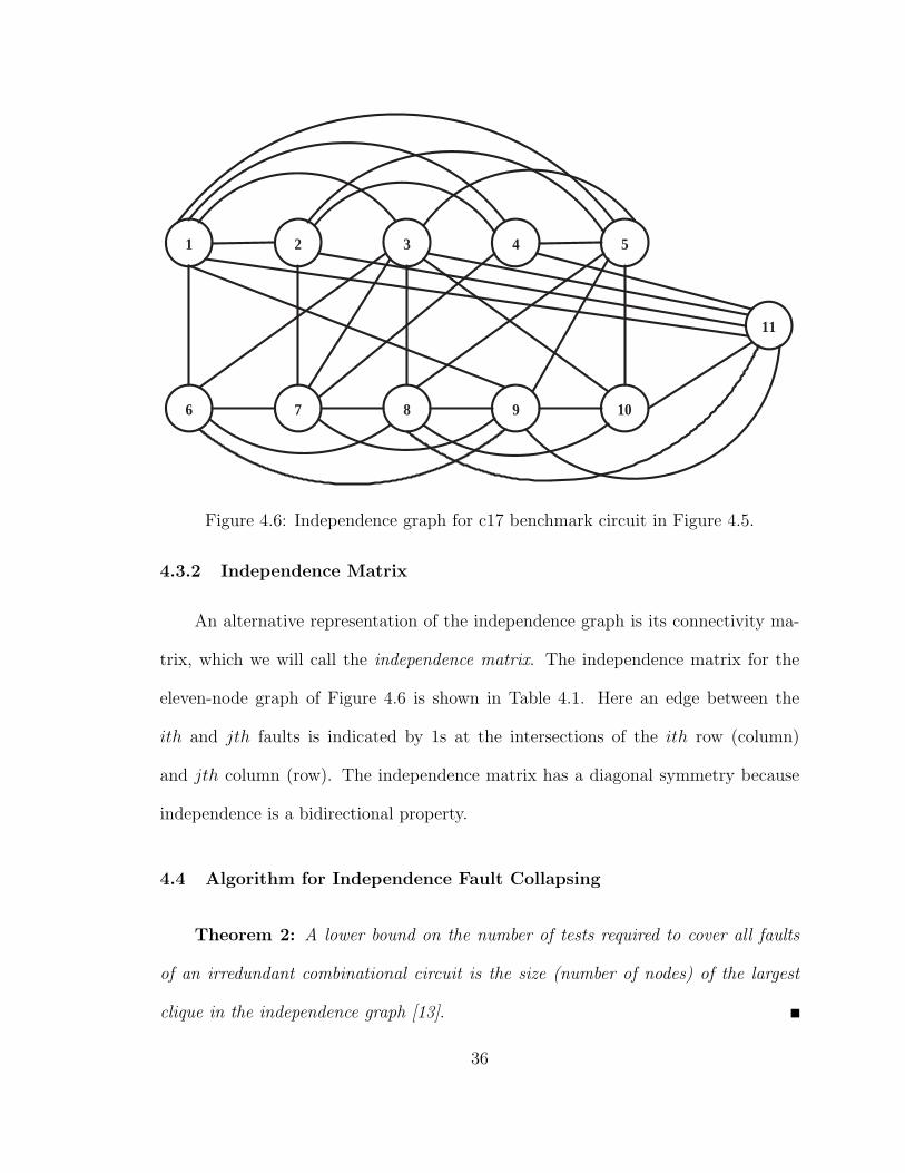
For the c17 benchmark circuit of Figure 4.5 we have a set of eleven faults, num-

bered 1 through 11 in the figure, obtained after functional dominance collapsing. We

construct the independence graph of Figure 4.6 where each fault is represented as a

node and an undirected edge between two nodes indicates the independence of the

corresponding faults. The edges in the independence graph represent functional in-

dependences and were found using the ATPG-based procedure of Figure 4.4(b). The

ATPG used was HITEC [58]. Since this graph is small, we can easily identify several

largest cliques of size four. Such identification will be impossible for large circuits

due to the high complexity of the maximum clique identification problem [12]. The

heuristic algorithm of Subsection 4.4 is found to work well in such cases.

In general, for large circuits one must rely only on structural independences and,

therefore, the independence graph will be only partially complete. This will affect

the minimality of the tests. In the following discussion, however, we will assume that

all edges of the independence graph are known.

35

1 2 3 4 5

6 7 8 9 10

11

Figure 4.6: Independence graph for c17 benchmark circuit in Figure 4.5.

4.3.2 Independence Matrix

An alternative representation of the independence graph is its connectivity ma-

trix, which we will call the independence matrix. The independence matrix for the

eleven-node graph of Figure 4.6 is shown in Table 4.1. Here an edge between the

ith and jth faults is indicated by 1s at the intersections of the ith row (column)

and jth column (row). The independence matrix has a diagonal symmetry because

independence is a bidirectional property.

4.4 Algorithm for Independence Fault Collapsing

Theorem 2: A lower bound on the number of tests required to cover all faults

of an irredundant combinational circuit is the size (number of nodes) of the largest

clique in the independence graph [13].

36

Table 4.1: Independence matrix for c17 benchmark circuit in Figure 4.5.

Fault 1 2 3 4 5 6 7 8 9 10 111 0 1 1 1 1 1 0 0 1 0 12 1 0 0 1 1 0 1 0 0 0 13 1 0 0 0 1 1 1 1 0 1 14 1 1 0 0 1 0 1 0 0 0 15 1 1 1 1 0 0 0 1 1 1 06 1 0 1 0 0 0 1 1 1 0 07 0 1 1 1 0 1 0 1 1 0 08 0 0 1 0 1 1 1 0 1 1 19 1 0 0 0 1 1 1 1 0 1 110 0 0 1 0 1 0 0 1 1 0 111 1 1 1 1 0 0 0 1 1 1 0

A clique is defined as a fully-connected subgraph, i.e., a subgraph in which every

node is connected to every other node. Thus, the largest clique in the independence

graph of Figure 4.6 has a size 4. This is shown in Figure 4.7 by a dashed line enclosure.

The above theorem follows from the fact that a test for a fault in the clique will not

detect any other fault in that clique.

Notice that Theorem 2 is valid even for an independence graph where the in-

dependence edges are only partially known. However, the size of the clique will be

largest when all independences are known. In that case the lower bound on the

number of tests will be smallest.

Finding the largest clique in a graph (or even the chromatic number, i.e., the size

of the largest clique) is an NP-complete problem [11, 12]. Therefore, we will not try

to determine it directly. Besides, our aim is to find the targets for test generation that

will lead to the minimal test set. Heuristically, two nodes that are not connected by

an independence edge can form a single node whose label combines the fault labels

of both nodes. Then, all nodes that have edges connecting to the two nodes will have

37

1 2 3 4 5

6 7 8 9 10

11

Figure 4.7: Largest clique in the independence graph of Figure 4.6.

edges to the combined node. This collapsing procedure ends when the graph becomes

fully-connected. However, depending on the order in which the nodes are collapsed

the size of the collapsed graph can vary. We have found that for larger circuits it

produces non-optimum results. For improved collapsing, we propose a new heuristic

method in the next subsection.

Once the independence graph is collapsed into a fully-connected graph (a single

clique), the faults in each node label may require one or more tests. However, the

concurrent tests generated for one node cannot completely detect all faults in any

other node. Suppose the ith node contains ki faults, then any pair of those faults can

be detected by a concurrent test. Therefore, we have

38

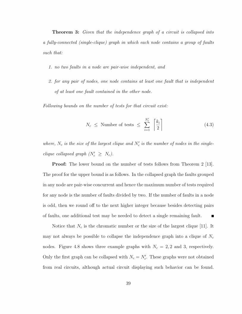
Theorem 3: Given that the independence graph of a circuit is collapsed into

a fully-connected (single-clique) graph in which each node contains a group of faults

such that:

1. no two faults in a node are pair-wise independent, and

2. for any pair of nodes, one node contains at least one fault that is independent

of at least one fault contained in the other node.

Following bounds on the number of tests for that circuit exist:

Nc ≤ Number of tests ≤N ′

c∑

i=1

⌈

ki

2

⌉

(4.3)

where, Nc is the size of the largest clique and N ′

c is the number of nodes in the single-

clique collapsed graph (N ′

c ≥ Nc).

Proof: The lower bound on the number of tests follows from Theorem 2 [13].

The proof for the upper bound is as follows. In the collapsed graph the faults grouped

in any node are pair-wise concurrent and hence the maximum number of tests required

for any node is the number of faults divided by two. If the number of faults in a node

is odd, then we round off to the next higher integer because besides detecting pairs

of faults, one additional test may be needed to detect a single remaining fault.

Notice that Nc is the chromatic number or the size of the largest clique [11]. It

may not always be possible to collapse the independence graph into a clique of Nc

nodes. Figure 4.8 shows three example graphs with Nc = 2, 2 and 3, respectively.

Only the first graph can be collapsed with Nc = N ′

c. These graphs were not obtained

from real circuits, although actual circuit displaying such behavior can be found.

39

3

1 2

342, 41, 3

1

6

2 1, 3

6

1 2

3

1, 3

graphIndependence Maximal clique

cNsize, graphCollapsed

2

2

3

Collapsed graphcN’size,

2

3

4

45

2, 5

4

4

5

2, 5

4

Figure 4.8: Examples of independence graphs, cliques and collapsed graphs.

When N ′

c > Nc, the circuit will essentially require more than Nc tests and the lower

bound of Theorem 2 will be exceeded. An example is the four-bit ALU circuit for

which an independent fault set size (Nc) of 11 has been identified [14] but the circuit

needs at least 12 tests for detecting all faults.

When the independence graph is collapsed into N ′

c nodes, Theorem 3 shows that

the number of tests a node contributes has an upper bound. A good collapsing

algorithm will attempt to group faults such that the number of tests contributed by

40

each node is minimized. In the following we use similarity heuristics to find “good”

groupings.

4.4.1 Definitions

Before we discuss the independence fault collapsing algorithm, we will define two

metrics that can be directly computed from the independence matrix:

Definition 3: Degree of independence (DI): The degree of independence of a

fault i is the number of edges attached to its fault node and is computed by adding

all the elements of either the ith row or the ith column of the independence matrix:

DI(fault − i) =N

∑

j=1

xij =N

∑

j=1

xji (4.4)

where xij is the element belonging to the ith row and jth column of the N × N

independence matrix (N is the number of faults). Thus, for the fourth fault, the

matrix of Table 4.1 gives:

DI(4) =11∑

i=1

x4i = 5 (4.5)

The DI for each fault of circuit in Figure 4.5 is shown in Table 4.2.

Definition 4: Similarity metric (SIM): This is a measure defined for a pair of

faults that determines how similar they are in their independence and concurrent-

testability with respect to the entire fault set of the circuit:

SIM(fault − i, fault − j) = Nxij + (1 − xij)N

∑

k=1

|xik − xjk| (4.6)

41

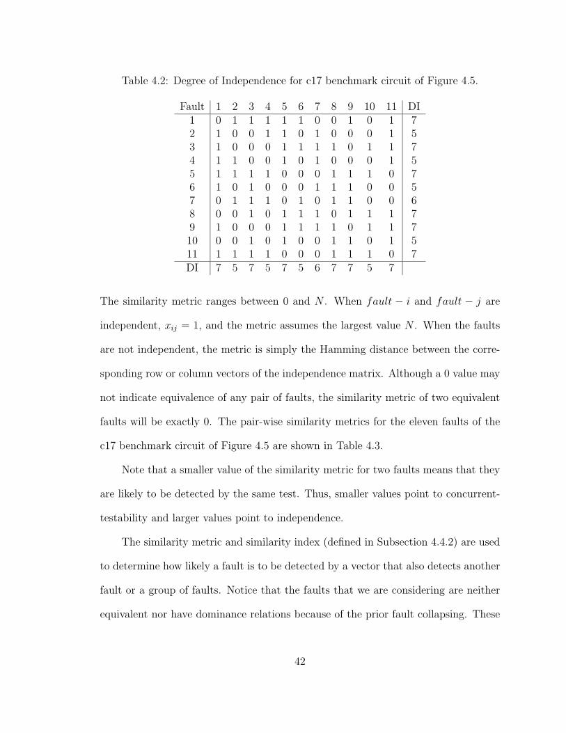
Table 4.2: Degree of Independence for c17 benchmark circuit of Figure 4.5.

Fault 1 2 3 4 5 6 7 8 9 10 11 DI1 0 1 1 1 1 1 0 0 1 0 1 72 1 0 0 1 1 0 1 0 0 0 1 53 1 0 0 0 1 1 1 1 0 1 1 74 1 1 0 0 1 0 1 0 0 0 1 55 1 1 1 1 0 0 0 1 1 1 0 76 1 0 1 0 0 0 1 1 1 0 0 57 0 1 1 1 0 1 0 1 1 0 0 68 0 0 1 0 1 1 1 0 1 1 1 79 1 0 0 0 1 1 1 1 0 1 1 710 0 0 1 0 1 0 0 1 1 0 1 511 1 1 1 1 0 0 0 1 1 1 0 7DI 7 5 7 5 7 5 6 7 7 5 7

The similarity metric ranges between 0 and N . When fault − i and fault − j are

independent, xij = 1, and the metric assumes the largest value N . When the faults

are not independent, the metric is simply the Hamming distance between the corre-

sponding row or column vectors of the independence matrix. Although a 0 value may

not indicate equivalence of any pair of faults, the similarity metric of two equivalent

faults will be exactly 0. The pair-wise similarity metrics for the eleven faults of the

c17 benchmark circuit of Figure 4.5 are shown in Table 4.3.

Note that a smaller value of the similarity metric for two faults means that they

are likely to be detected by the same test. Thus, smaller values point to concurrent-

testability and larger values point to independence.

The similarity metric and similarity index (defined in Subsection 4.4.2) are used

to determine how likely a fault is to be detected by a vector that also detects another

fault or a group of faults. Notice that the faults that we are considering are neither

equivalent nor have dominance relations because of the prior fault collapsing. These

42

Table 4.3: Similarity Metrics for c17 benchmark circuit of Figure 4.5.

Fault 1 2 3 4 5 6 7 8 9 10 111 0 11 11 11 11 11 3 4 11 4 112 11 0 4 11 11 6 11 6 4 6 113 11 4 0 4 11 11 11 11 0 11 114 11 11 4 0 11 6 11 6 4 6 115 11 11 11 11 0 4 3 11 11 11 06 11 6 11 6 4 0 11 11 11 4 47 3 11 11 11 3 11 0 11 11 5 38 4 6 11 6 11 11 11 0 11 11 119 11 4 0 4 11 11 11 11 0 11 1110 4 6 11 6 11 4 5 11 11 0 1111 11 11 11 11 0 4 3 11 11 11 0

measures differ from the “level of similarity” defined in the literature [65], which

determines how close a fault is to being equivalent or dominant with respect to another

fault.

4.4.2 Independence Fault Collapsing Algorithm

Now that we have defined the metrics that we will use for collapsing, let us discuss

the independence fault collapsing algorithm in detail. This algorithm collapses the

graph or groups the faults into sets of concurrently-testable faults. At this point

we already have the independence matrix generated. We will use this matrix for

collapsing the faults.

Algorithm: Similarity-Based Independence Fault Collapsing

1. Compute the degree of independence for each fault.

2. Arrange the faults in order of decreasing degree of independence.

3. Compute the similarity metric for each pair of faults.

43

4. Starting with an empty graph, place faults in the new order of decreasing degree

of independence. Create the first node consisting of the fault with the highest

degree of independence.

5. Until all faults have been placed, place a fault F with the same or the next

highest degree of independence:

• Compute a similarity index for F for each existing node i as:

MaxKk=1

SIM(F, kth fault of node i)

where K is the number of faults in node i.

• If the similarity index for all nodes is N (maximum value), i.e., all nodes

contain at least one fault that is independent of F , then create a new

node for F . Otherwise, place F in the node for which it has the smallest

similarity index.

This algorithm, based on a “similarity heuristic”, tries to group those faults to-

gether that are likely to have a single concurrent test. The algorithm groups faults

into nodes such that the similarity metrics among faults within each group are mini-

mized. Recall that the similarity metric is a pair-wise measure. Its minimum value,

0, signifies that the two faults, although not equivalent, are close to being equivalent.

Larger values of the similarity metric point to the reducing size of the common tests

for the two faults. The maximum possible value, which equals the total number of

faults (N), indicates a null set for the common tests, i.e., the faults are independent.

Thus, by grouping the faults together that are “nearly” equivalent we increase the

44

Table 4.4: Step 1: Computation of degree of independence (DI) for each fault.

Fault 1 2 3 4 5 6 7 8 9 10 11 DI1 0 1 1 1 1 1 0 0 1 0 1 72 1 0 0 1 1 0 1 0 0 0 1 53 1 0 0 0 1 1 1 1 0 1 1 74 1 1 0 0 1 0 1 0 0 0 1 55 1 1 1 1 0 0 0 1 1 1 0 76 1 0 1 0 0 0 1 1 1 0 0 57 0 1 1 1 0 1 0 1 1 0 0 68 0 0 1 0 1 1 1 0 1 1 1 79 1 0 0 0 1 1 1 1 0 1 1 710 0 0 1 0 1 0 0 1 1 0 1 511 1 1 1 1 0 0 0 1 1 1 0 7DI 7 5 7 5 7 5 6 7 7 5 7

possibility of finding a single concurrent test for the group. Let us see the example

of the c17 benchmark circuit of Figure 4.5.

The degree of independence is first calculated for each fault as shown in Table 4.4.

The faults are then arranged in order of decreasing degree of independence (Table 4.5).

The order of the faults is as follows (value shown in parenthesis is the degree of

independence): 1(7), 3(7), 5(7), 8(7), 9(7), 11(7), 7(6), 2(5), 4(5), 6(5), 10(5). Then,

the similarity metric is calculated for each pair of faults (Table 4.6).

The step by step details of the collapsing procedure are shown in Figure 4.9. The

number shown inside the node is the fault number while the number shown outside

the node is the similarity index for the next fault with that node. We start with fault

1 and create the first node for it. Since SIM(3, 1) = 11 (indicating independence),

we create a new node for fault 3. Similarly, a new node is created for fault 5 because

it is independent of both faults 1 and 3. Next, fault 8 is placed in the node with

fault 1 because it has the lowest similarity index for that node. Proceeding in similar

45

Table 4.5: Step 2: Faults ordered according to decreasing degree of independence.

Fault 1 3 5 8 9 11 7 2 4 6 10 DI1 0 1 1 0 1 1 0 1 1 1 0 73 1 0 1 1 0 1 1 0 0 1 1 75 1 1 0 1 1 0 0 1 1 0 1 78 0 1 1 0 1 1 1 0 0 1 1 79 1 0 1 1 0 1 1 0 0 1 1 711 1 1 0 1 1 0 0 1 1 0 1 77 0 1 0 1 1 0 0 1 1 1 0 62 1 0 1 0 0 1 1 0 1 0 0 54 1 0 1 0 0 1 1 1 0 0 0 56 1 1 0 1 1 0 1 0 0 0 0 510 0 1 1 1 1 1 0 0 0 0 0 5DI 7 7 7 7 7 7 6 5 5 5 5

ways, all other faults are placed as shown in Figure 4.9. The last graph in Figure 4.9

is the final collapsed graph, which contains just four nodes. The groups are also

shown in Table 4.7. The edges in the collapsed graph indicate that a minimal set

of tests for faults in any node cannot completely cover the faults in any other node.

Formula 4.3 gives the lower and upper bounds on the number of test vectors as 4 and

7, respectively. In Chapter 5, we will see that concurrent test generation provides

four vectors for this circuit.

We make several observations about the independence collapsing algorithm of

this section:

1. The algorithm will always terminate with a collapsed graph because the faults

are sequentially placed on the collapsed graph and the placement procedure

results in a definite placement of a fault before next fault is placed.

46

Table 4.6: Step 3: Computation of similarity metric for each pair of faults.

Fault 1 3 5 8 9 11 7 2 4 6 101 0 11 11 4 11 11 3 11 11 11 43 11 0 11 11 0 11 11 4 4 11 115 11 11 0 11 11 0 3 11 11 4 118 4 11 11 0 11 11 11 6 6 11 119 11 0 11 11 0 11 11 4 4 11 1111 11 11 0 11 11 0 3 11 11 4 117 3 11 3 11 11 3 0 11 11 11 52 11 4 11 6 4 11 11 0 11 6 64 11 4 11 6 4 11 11 11 0 6 66 11 11 4 11 11 4 11 6 6 0 410 4 11 11 11 11 11 5 6 6 4 0

Table 4.7: Independence fault collapsing of c17 faults.

Fault FaultsGroup No. (see Figure 4.5)

1 1, 82 2, 3, 93 4, 6, 104 5, 7, 11

47

1,8

3, 9, 2

5, 11, 7

4, 6, 10

1

3

5 1, 8

3

5

1 1

3

1, 8

3, 9

5 1, 8

3, 9

5, 11

1, 8

3, 9

5, 11, 7 1, 8

3, 9, 2

5, 11, 7

1,8

3, 9, 2

5, 11, 7

4

1,8

3, 9, 2

5, 11, 7

4, 6

11 11

11

4

11

11 11 11

0

11 0

11

11 3

11

11 11

4

11 11

11

11 11

11

6

11

11

11

6

Figure 4.9: Steps 4 and 5: Collapsing the independence graph of c17.

48

2. The size of the collapsed graph cannot be smaller than the maximal clique size

Nc (chromatic number) of the independence graph. This is because no two

faults that are independent can be placed in the same node.

3. Whenever a circuit requires more tests than the lower bound of Theorem 2 or

3, the collapsed graph will definitely have more than Nc nodes, i.e,. N ′

c > Nc.

This happens when the independence graph has more than one maximal clique

and those cliques are connected in certain ways. While a complete analysis of

such graphs may be complex, the phenomenon is illustrated by the examples of

Figure 4.8.

4.4.3 ALU Example

The algorithm of Section 4.4.2 was applied to the 74181 4-bit ALU circuit of

Figure 4.10. The Exclusive-OR gates in the circuit were expanded as four NAND

gates each as the ATPG program [58] and fault simulator [57] used for generating the

matrix did not recognize XOR gates. The independence matrix was generated for the

84 dominance collapsed faults shown in Figure 4.10 (92 faults are obtained through

functional dominance collapsing [71] of which 8 redundant faults are removed). The

independence fault collapsing procedure collapsed the 84 faults into 12 nodes. These

groups are shown in Table 4.8. Chapter 5 shows that 12 tests are obtained for the

ALU circuit.

The principal idea of the collapsing algorithm is to group those faults together

that are likely to have a concurrent test. The similarity index and degree of inde-

pendence play important roles in this algorithm. Otherwise, the grouping of faults

49

c_n

27

6

26

75

8 20

30

16

1513

14

22

33

4 18

31

2

36

s3s2s1s0

b3

a3

b2

a2

a0

b0

a1

b1

38

23

12

119

10

21

29

46

45

44

42

41

40

2437

17

51

50

49

35

32

39

19

43

4748

525453

m

f3n

pn

gn

f2n

a=b

f1n

f0n

56 58 59 57

25

28

31

34

61

60

55

64

67 65

62

78 79

68

70

69

71

7372

74

77

76

75

8182

8380

84

stuck−at−1

stuck−at−0

c_n+4

6366

Figure 4.10: ALU dominance collapsed faults [71].

50

Table 4.8: Independence collapsed fault sets for 4-bit ALU.

Node Maximum No. ofNo. similarity Faults Fault numbers (see Figure 4.10)

index

1 21 5 53, 58, 72, 66, 212 29 3 56, 64, 173 41 8 54, 48, 59, 73, 70, 67, 23, 64 37 3 55, 63, 515 43 5 34, 77, 10, 14, 366 49 6 61, 74, 42, 46, 50, 387 49 7 31, 76, 78, 16, 80, 39, 608 38 14 52, 47, 43, 57, 30, 71, 69, 68, 33, 65, 19, 79, 84, 39 47 8 28, 75, 29, 22, 18, 83, 8, 4410 41 8 24, 25, 27, 4, 12, 81, 7, 4011 43 8 62, 26, 32, 2, 13, 5, 9, 4912 36 9 20, 82, 35, 41, 45, 15, 11, 1, 37

could have been done almost arbitrarily after we found the largest clique in the in-

dependence graph using any available maximum clique program. To illustrate the

effectiveness of our independence collapsing algorithm, we reworked the ALU exam-

ple. Appendix A shows the collapsed faults sets for the ALU circuit of Figure 4.10

without ordering the faults according to decreasing degree of independence. We were

able to collapse the graph to a low of 15 nodes, and we obtained a test set of 17 vectors

for those 15 groups of faults. This shows the importance of ordering the faults before

we start the collapsing procedure.

4.5 Simulation-Based Independence Fault Collapsing

There are practical difficulties in implementing the procedures explained in Sec-

tion 4.4 for large circuits. First, functional dominance fault collapsing [71], used prior

to independence collapsing, is based on ATPG and is complex (the time taken for

51

functional dominance collapsing for the ALU circuit was approximately 45 minutes).

Second, the independence graph generation procedure of Section 4.2.3 is also based

on ATPG (the time taken to generate the independence matrix was approximately

50 minutes). In this section, we give an alternative procedure using a conventional

fault simulator for generating the independence matrix. The only requirement is that

the fault simulator should simulate without fault dropping, as is usually needed in

diagnosis applications. The technique has been described in a recent paper [8].

4.5.1 Algorithm

1. Start with a fully-connected independence graph for an equivalence collapsed

fault set (structural collapsing only), i.e., assume initially all faults are indepen-

dent of each other.

2. Simulate random vectors without fault dropping to remove edges between faults

detected by the same vector. Stop the random vector simulation when a large

number of vectors do not remove any new edges.

3. Apply the independence fault collapsing algorithm of Section 4.4.2 to the gen-

erated independence matrix.

The procedure is illustrated for the 4-bit ALU (74181) circuit. We begin with the

structural equivalence collapsed fault set as obtained from any ATPG or fault simula-

tion program. For the 4-bit ALU circuit this set contains 301 stuck-at faults including

8 redundant faults. Exclusive-OR gates in the circuit were expanded as four NAND

gates each. Assuming no prior information about the concurrent detectability (com-

patibility) of faults, initially a fully connected independence graph was constructed

52

Table 4.9: Simulation-based independence fault collapsing for 4-bit ALU (74181)circuit.

Group Number Maximum SimilarityNo. of faults index

1 9 962 15 1273 11 944 6 1085 11 1266 17 1367 11 1248 16 1249 16 12710 22 11511 22 11112 56 10413 81 104

for 301 faults. This graph contains 301 × 301 = 90, 601 edges. The fault simulator

HOPE [55] was used to simulate random vectors without fault dropping. The upper

curve in Figure 4.11 shows the fault coverage reaching 293 (all detectable faults) at

vector number 193. All edges among the faults detected by each vector were deleted

from the independence graph, reducing the number of edges from 90,601 as shown by

the lower curve in Figure 4.11. For example, the first vector detected 73 faults and

caused the deletion of 73 × 73 = 5, 329 edges. The simulation was stopped at 2,000

random vectors when it was found that about 200 vectors did not remove any new

edge. This left 20,004 or about 22% of the edges. In this graph, there were eight nodes

that were still connected to all other nodes giving them a degree of independence 301.

An ATPG [54] was used to derive tests or prove redundancy. Since these faults were

found to be redundant, the corresponding nodes and all edges attached to them were

removed leaving 293 nodes.

53

0

25000

50000

75000

100000

0 500 1000 1500 2000 2500

Random vectors

Nu

mb

er o

f ed

ges

0

80

160

240

320

Fau

lts

det

ecte

d

90601 Faults detected (293)

Number of edges in graph (20004)

301

Figure 4.11: Random vector fault simulation to obtain independence graph of 4-bitALU.

The similarity-based independence collapsing algorithm of Section 4.4.2 grouped

293 faults into 13 groups with sizes ranging from 6 to 81 faults. The groups are shown

in Table 4.9. Chapter 5 shows that 12 tests were generated for these 13 groups.

It has to be noted that the number of groups generated here is more than the

optimal result of 12 because when random vectors are used, not all fault-pair relations

are found. Some pairwise concurrent faults may still be treated as independent faults

just because the set of random vectors did not have a vector that would detect these

faults at the same time. Hence, the collapsing procedure may generate more groups.

So, Equation 4.3 would now give a different higher bound on the number of tests.

54

Table 4.10: Independence fault collapsing of ripple-carry full-adders.

Circuit Independence Collapse Groups

1-b adder 52-b adder 54-b adder 58-b adder 716-b adder 732-b adder 7

4.5.2 More Results

The algorithm of Section 4.4.2 was applied to ripple-carry full-adder circuits

ranging from 1-bit to 32-bits. The simulation-based method of graph generation was

used. The results are shown in Table 4.10. The adders are known to have a minimal

set of 5 tests irrespective of their size [48]. From Table 4.10 it can be seen that the

collapsing procedure produced the minimal result until the 4-bit adder and the results

slightly deviated for the remaining adder circuits.

Table 4.11 shows the independence fault collapsing results for the ISCAS85 com-

binational benchmark circuits. The last column shows the total time required for

generating the independence matrix as well as collapsing the graph. It can be seen

from the table that the time required increases as the size of the circuit increases.

This is because the technique is based on fault simulation and as the circuit size in-

creases, the number of faults in the circuit increases and so simulation time increases.

But, this increase is linear or quadratic and not exponential.

The concurrent test generation results for these circuits are presented in the next

chapter.

55

Table 4.11: Independence fault collapsing on ISCAS85 benchmark circuits.

Circuit Independence Collapse Groups CPU Time (s)*

c17 4 0.04c432 30 2.0c499 52 3.4c880 24 4.3c1355 84 6.9c1908 106 10.9c2670 81 16.3c3540 107 24.7c5315 92 41.8c6288 23 64.9c7552 190 62.9

* Sun Ultra 5

4.6 An Alternative Method for Independence Fault Collapsing

In this section we propose another method for independence fault collapsing

which is based on cliques. This method uses the same algorithm proposed in Sec-

tion 4.4.2, but instead of starting with an empty graph in step 4, we start with a

maximum clique. This maximum clique is determined prior to applying the collaps-

ing algorithm. There are several algorithms proposed in literature for finding the

maximum clique [25, 60, 53]. We use a tool called Reactive Local Search solver [17]

which is based on the algorithm of Battiti and Protasi [18] for finding a maximal

clique of a graph. The input file for this tool is in the DIMACS (Center for Dis-

crete Mathematics and Theoretical Computer Science) [31] format. The details of

the DIMACS format are given in Appendix B.

This method was applied to the c17 benchmark circuit of Figure 4.5. A maximum

clique was found by using the Reactive Local Search solver [17]. One run of the tool

gave the maximum clique formed by faults 6, 7, 8 and 9. Then steps 1, 2 and 3 from

56

11 3

4

11

11

11

11

0

6

8

7

9

6

8

7, 1

9

4 11

11

11

4

11

11

11

6

8

7, 1

9, 3

6, 5

8

7, 1

9, 3

11 11

6

4

11

6

11

11

6, 5 ,11

8

7, 1

9, 3

6, 5, 11

8

7, 1

9, 3 2

11 5

11

11

6, 5, 11

8, 4

7, 1, 10

9, 3, 2

6, 5, 11

8, 4

7, 1

9, 3, 2

Figure 4.12: Independence collapsing of c17 faults starting from a known clique.

57

Table 4.12: Results for the c17 circuit.

Fault Faults ConcurrentGroup No. (see Figure 4.5) test vector

1 6, 5, 11 011002 7, 1, 10 100113 8, 4 101004 9, 3, 2 01111

the algorithm in section 4.4.2 were performed. For steps 4 and 5, this clique was used

as the starting graph. While performing steps 4 and 5, the faults in the starting clique

were omitted as they were already grouped. This collapsing procedure is shown in

Figure 4.12. Notice that this collapsing method produced different groups than the

previously obtained groups. Also the concurrent test generation for these new groups

came up with a different set of four (minimal) tests, which are shown in Table 4.12.

For the 74181 circuit, we used the 301-node independence graph obtained by the

simulation-based technique in Section 4.5. Reactive Local Search solver [17] found a

clique of size 11 which agrees with the lower bound (number of independent faults)

for this circuit as given in [14]. But, the minimum number of tests required for this

circuit is 12 which is greater than the lower bound [14].

The advantage of this method is that we already have the nodes, and we just

have to place the remaining faults into these nodes without forming new nodes unless

necessary. So we would always have a chance to come up with the minimum number

of nodes. But, the problem of finding the maximal clique is NP-hard and so the tool

cannot find the maximal clique in a given small time (the tool was run on the server

provided by the website, which allowed a maximum run time of only 600 seconds for

a given problem). So, we did not apply this method to the other benchmark circuits.

58

Chapter 5

Concurrent Test Generation

Independence fault collapsing discussed in Chapter 4 helped group the faults

that are likely to be detected by the same test vector into a single group. Now that

the faults are grouped together, we need a technique to find a single test that would

detect all or most of the faults in a group. In this chapter we define a new type

of test, called “concurrent test,” for a combinational circuit. Also, we present new

techniques to generate these concurrent tests. Some techniques and examples of this

chapter have appeared in recent papers [8, 32].

Definition 5: Given a set of target faults, a concurrent test is an input vector

that detects all (or most) faults in the set.

When concurrent tests are generated for fault sets obtained from independence

fault collapsing, minimal or near-minimal tests can be expected. Although the general

problem of concurrent test generation relates to a set of faults, for simplicity, we will

consider two faults, F1 and F2. Figure 5.1 shows the Boolean satisfiability and

multi-valued ATPG formulations of the concurrent test problem. C0 is the fault-free

function and Ci is the function with fault Fi permanently injected. Any vector that

satisfies the following equation is a concurrent test for F1 and F2. This is the Boolean

satisfiability solution shown in Figure 5.1(a).

(C0 ⊕ C1).(C0 ⊕ C2) = 1 (5.1)

59

0

1

C

C

C

C2

0

test vector

(a) Boolean satisfiability.

1

0

1

Concurrenttest vector

Concurrent

0/1

0/1

0/1

(b) Five or nine valued ATPG.

1

fault F1

fault F2

CUT C0

CUT C

CUT C

0

Figure 5.1: Generation of concurrent test.

60

Figure 5.1(b) shows a multi-valued ATPG solution. Notice that the ATPG re-

quires three copies of the circuit (CUT) and the detection of a multiple fault whose

components, F1 and F2, are in two separate copies. There are two ways of generating

a concurrent test. One way is to use a known method of modeling a multiple fault [51]

as a single fault for any available ATPG program. The disadvantage of this method

is that the circuit the ATPG program has to deal with is now n+1 times larger when

the concurrent fault set has n faults. The second method, which does not duplicate

the circuit, is given in the next section.

5.1 The Concurrent-D Algebra

Consider two faults, F1 and F2. The state of any line in the circuit is either

(1) unaffected by both faults, (2) affected by F1, (3) affected by F2, or (4) affected

by both F1 and F2. In the first case the line assumes a value from the set 0, 1, X.

In the second case we denote it by D1 or D1, where D1 has the same meaning as in

the D-algorithm [69]. Similarly, for the third case the line value is denoted as D2 or

D2. In the fourth case, where both faults affect the line, its state is denoted by D12

or D12. Thus, there are nine values that a line can have. For a two-input AND gate,

the function is shown in Table 5.1.

Figure 5.2 shows the concurrent test generation for the c17 benchmark circuit of

Figure 4.5. Faults 2, 3 and 9 shown in Figure 5.2 are all of stuck-at-1 type and were

grouped together using the independence fault collapsing algorithm of Section 4.4.2

and are shown in Table 4.7. The concurrent test vector generated for faults 2, 3 and

9 is “01111”. Table 5.2 shows the concurrent test vectors for all the groups of the c17

circuit.

61

Table 5.1: Output of a 2-input AND gate with concurrent-D algebra.

AND I N P U T T W O0 1 X D1 D2 D1 D2 D12 D12

I 0 0 0 0 0 0 0 0 0 0N 1 0 1 X D1 D2 D1 D2 D12 D12

P X 0 X X X X X X X XU D1 0 D1 X D1 D12 0 D2 D12 D2

T D2 0 D2 X D12 D2 D1 0 D12 D1

D1 0 D1 X 0 D1 D1 0 0 D1

O D2 0 D2 X D2 0 0 D2 0 D2

N D12 0 D12 X D12 D12 0 0 D12 0E D12 0 D12 X D2 D1 D1 D2 0 D12

2 - 1

3 - 1

9 - 1

0

1

1

1

1

D 2 D 2

D 3

D 9

D 3

D 9

D 23

D 39 0

Figure 5.2: Concurrent test generation for c17.

Table 5.2: Concurrent test vectors for c17.

Fault Faults ConcurrentGroup No. (see Figure 4.5) test vector

1 1, 8 100102 2, 3, 9 011113 4, 6, 10 101014 5, 7, 11 x1010

62

Table 5.3: Concurrent test generation for the 4-bit ALU (74181) circuit.

Node Number of faults Test vectorsNo. Total Targeted Detected from Cumulative (Input order as in

this node other nodes coverage Figure 4.10)

1 5 5 5 6 11 010011110100012 3 3 3 2 16 010011111101013 8 7 7 3 26 010111010000014 3 3 3 3 32 101x01010100005 5 3 3 4 39 101001010110006 6 6 6 2 47 111110000010017 7 4 4 3 54 111000001000008 14 11 11 1 66 111001101010119 8 6 5 1 72 1001010011010110 8 4 3 2 77 1x10101110110011 8 3 3 1 81 0101000010110012 9 2 2 1 84 1x011110001100

5.1.1 Four-Bit ALU (74181)

The circuit diagram of the four-bit ALU (74181) used in this work is shown in

Figure 4.10. For concurrent test generation, nodes were targeted in the order they are

listed in Table 4.8. The result is shown in Table 5.3. For example, the node processed

first has 5 faults, all of which are targeted simultaneously. We got a test vector, shown

in the last column, that detected all 5 of the targeted faults. Fault simulation of that

vector showed that it detected 6 faults from other nodes as well, giving a cumulative

coverage of 11. Although there were very few don’t care bits in these vectors they

were enumeratively filled during fault simulation and the combination of values that

covered most extra faults was retained. The don’t care bits shown in Table 5.3 are

those that did not affect the fault coverage. For subsequent nodes, already detected

faults were not targeted. Thus, node 3, which has 8 faults, only provided 7 target

faults. By the time we reached the twelfth node, 7 of its faults had been detected.

63

Table 5.4: Test sets for ALU.

ATPG Number of Tests

Concurrent ATPG 12Atalanta [54] 23Random [55] 31Hitec [58] 36Fastest [50] 37Gentest [28] 42

However, one fault from a previous node was left over. All three were detected by the

twelfth vector. The set of 12 vectors obtained in Table 5.3 is the smallest possible for

this circuit [14, 42]. Table 5.4 lists the number of test vectors generated for the ALU

circuit by different ATPG programs. The random vector generator within the fault

simulator HOPE [55] was used for random ATPG. It can be seen from the results in

Table 5.4 that the test set obtained by concurrent ATPG is almost 50% smaller than

the best result by any conventional ATPG.

Although the results in this section were obtained using the concurrent-D algebra,

an ATPG program using this technique has not been completed. The reported results

were obtained by a manual application of the algorithm.

5.2 Simulation Based Concurrent Test Generation

The use of the concurrent D-algebra of Section 5.1 requires a new ATPG program

that may not be readily available to a user. In this section, we give an alternative

procedure using a conventional fault simulator and single-fault ATPG programs for

concurrent test generation. The only requirement is that the fault simulator should

simulate without fault dropping, as is usually needed in diagnosis applications.

64

5.2.1 Algorithm

Our objective is to generate a single test vector to cover all or most faults in each

group. The independence collapsing algorithm of Section 4.4.2 orders the faults within

each group in the order of their degree of independence (DI) given in Equation 4.4.

DI is simply the number of edges attached to a fault node in the independence graph.

A fault with higher DI is likely to be detectable by a smaller set of vectors. For

each group, we select the fault with highest DI, i.e., the first fault in the group, and

derive all test vectors for it. We then use a fault simulator to select a vector that

detects most faults in the group. If more vectors than one detect the same number

of faults within the group, then we select the one that detects most faults outside

the group as well. The multiple test vector generation capability of Atalanta [54] and

fault simulation without fault dropping in HOPE [55] were used. Since the number

of test vectors for a fault can be very large and the vectors may contain don’t care

bits, we limited the number of vectors for a target fault to 250 and expanded each

vector with don’t cares into no more than 10 vectors.

We applied the above procedure to the 4-bit ALU circuit. The simulation based

independence fault collapsing had already grouped the faults into 13 sets. The above

heuristic produced one vector for each of the first 11 groups as shown in Table 5.5.

All 56 faults in group 12 were detected by these 11 vectors and the vector selected

for group 13 detected all faults that were not detected by the previous vectors.

5.2.2 Results

Table 5.6 shows the results of independence fault collapsing (number of fault

groups) and concurrent ATPG (number of vectors) for ripple-carry adders up to 32

65

Table 5.5: Simulation-based concurrent test generation for the 4-bit ALU (74181)circuit.

Group Number Test vectorNo. of faults (for bit order see Figure 4.10)

1 9 011000111111002 15 011011000001103 11 101001011110104 6 110110101000005 11 101101010110106 17 101001111010107 11 100101010011108 16 010001111010119 16 1110001001001110 22 1101110011010011 22 0101000110000112 56 No test needed.13 81 10101001110110

bits, the 4-bit ALU and the combinational benchmark circuits. For comparison,

single-fault ATPG results are given. The column “Dyn*” gives one of the best re-

ported results obtained by dynamic vector compaction [41]. “Min-Max” are the num-

bers of statically compacted and uncompacted vectors generated by Atalanta [54]. For

ripple-carry adders, the minimum number of vectors is 5, irrespective of the adder

size [48]. The number of concurrent ATPG vectors grows, though at a slower rate

than the compacted Atalanta vectors. The four-bit ALU result is optimum. For

several benchmarks, concurrent ATPG produced a minimal vector set. For others it

produced more vectors than the best reported [41]. The numbers of collapsed groups

indicate approximately how many vectors will be generated. For many circuits, the

number of groups would be reduced if we simulated more random vectors causing

66

Table 5.6: Concurrent ATPG test length.

Independence Number of vectorsCircuit Collapse Concurrent Single-fault ATPG

Groups ATPG Dyn* Min-Max

1-b adder 5 5 5-72-b adder 5 5 7-94-b adder 5 5 8-118-b adder 7 7 10-1516-b adder 7 9 13-2232-b adder 7 11 17-254-b ALU 13 12 22-40

c17 4 4 6-9c432 30 34 27 49-77c499 52 52 52 54-68c880 24 29 16 52-106c1355 84 84 84 85-109c1908 106 111 106 118-173c2670 81 92 44 106-192c3540 107 130 84 147-263c5315 92 104 37 114-224c6288 23 25 12 32-48c7552 190 198 73 209-358

* Dynamic compaction (Hamzaoglu and Patel [41])

deletion of additional independence links from the graph. Our concurrent ATPG re-

quires all vectors for a single fault and had to be restricted when there were too many

such vectors.

Figure 5.3 shows the graphical comparison of the test set sizes given in Table 5.6.

It can be seen from the graph that the concurrent ATPG technique performs better

than the single-fault ATPG but needs improvement to match the result of the dynamic

compaction technique in [41].

Table 5.7 shows the CPU time in seconds taken by concurrent ATPG, and com-

pares it against the CPU times taken by the dynamic compaction technique in [41].

67

Table 5.7: Test generation time.

Circuit Concurrent ATPG Dynamic Compaction [41](seconds)* (seconds)**

1-b adder 0.0852-b adder 0.0924-b adder 0.1038-b adder 0.18216-b adder 3.332-b adder 9.74-b ALU 11.4

c17 0.082c432 10.4 15c499 14.6 0.1c880 23.3 21.9c1355 34 0.9c1908 49.6 88.1c2670 57.6 47.1c3540 119.6 174.5c5315 216.3 748.6c6288 158.1 347.7c7552 360.7 663.8

* Sun Ultra 5 ** Pentium Pro PC

It can be seen from the results that for the smaller circuits, the dynamic compaction

technique performs better, but as the circuit size increases, concurrent ATPG tech-

nique performs far better than [41]. The time required for test generation for the

larger circuits is almost a third of the time taken by dynamic compaction. So we

can say that the test generation time for concurrent ATPG has a linear or quadratic

relationship with the size of the circuit, and dynamic compaction has an exponential

relationship. This is shown in the graph in Figure 5.4.

Overall we see that the concurrent ATPG technique performed well in generating

minimal test sets for a few of the benchmark circuits and in a time that was less than

what the dynamic compaction technique [41] took.

68

0

50

100

150

200

250

300

350

400

Circuits in the order of Table 5.6

Num

ber

of t

est

vect

ors

Minimum Concurrent ATPG Single-fault ATPG

Single-fault ATPG (no compaction)

Concurrent ATPG

Minimum Achieved (dynamic compaction)

Figure 5.3: Test set size comparison.

69

0

100

200

300

400

500

600

700

800

Circuits in the order of Table 5.7

CP

U s

econ

ds

Minimum Concurrent ATPG

Concurrent ATPG

Minimum Achieved (dynamic compaction)

Figure 5.4: Test generation time comparison.

70

Chapter 6

Conclusion

We have developed a new test generation methodology for combinational circuits

based on independence fault collapsing and concurrent test generation. The indepen-

dence fault collapsing algorithm grouped all the faults in the circuit into a minimum

set of independent fault subsets such that each fault subset mostly ended up having

just one test. The concurrent test generation algorithm actually generated a single

test for each group of faults.

The independence fault collapsing procedure collapsed the graph into a minimal

clique. But the process of finding the independence matrix was computationally

expensive. So, we presented another approach based on fault simulation for finding

the independence matrix. This technique was not computationally expensive but,

we had to deal with an incompletely specified matrix. This resulted in a larger set

of collapsed nodes, thus increasing the lower bound on the number of tests to be

generated.

The concurrent ATPG using the concurrent D-algebra produced a single test for

each subset of faults, thus generating a test set equal to the lower bound. But, this

procedure required the implementation of a new ATPG tool. Therefore, we presented

another approach to concurrent test generation based on fault simulation and single-

fault ATPG. This technique often produced satisfactory results.

71

The simulation based techniques were applied to the ISCAS85 combinational

benchmark circuits as well as to several ripple-carry adder circuits and a 4-bit ALU.

We saw that for smaller circuits, including the ALU, the techniques produced the

optimal result. Also, for some benchmark circuits, the optimal result was achieved.

The computational time was found to be far less compared to a dynamic compaction

techniques, which have also produced optimal results.

We can conclude that concurrent test generation produced compact tests when

combined with independence fault collapsing. Also, ATPG and set covering problems

have exponential time complexities and so, we cannot expect absolute optimality for

large circuits.

6.1 Future Work

The simulation-based algorithms for independence fault collapsing and concur-

rent test generation can be improved. The fault collapsing algorithm can be made

more dynamic in the sense that after collapsing, if a minimal clique is not formed,

flexibility needs to be given to go back and remove a fault from a group and place it

in some other group. The same flexibility can be provided during the concurrent test

generation process. The algorithms need to be made more efficient. A tool that would

implement the collapsing and test generation algorithms needs to be developed.

One other concern is about the memory required to store the independence ma-

trix. As the number of faults in the circuit increases, this requirement also increases.

Some alternative method of storing the matrix needs to be devised.

It is recommended that an ATPG program be implemented using the concurrent-

D algebra. Since the independence fault collapsing does not guarantee that a fault

72

group can be covered by exactly one test vector, the ATPG will need to make a

heuristic decision to drop some faults.

Another possibility that should be explored is to use the concurrent ATPG phase

of a simulation-based directed-search ATPG algorithm [7, 27].

Since the problem of finding the minimal test set is NP-hard, there will always

be that extra bit of work that one can do to keep on improving the results.

73

Bibliography

[1] M. Abramovici, M. A. Breuer, and A. D. Friedman, Digital Systems Testing andTestable Design. Piscataway, New Jersey: IEEE Press, 1994.

[2] M. Abramovici, J. J. Kulikowski, P. R. Menon, and D. T. Miller, “SMART and FAST:Test Generation for VLSI Scan-Design Circuits,” IEEE Design and Test of Computers,vol. 3, no. 4, pp. 43–54, Aug. 1986.

[3] P. Agrawal and V. D. Agrawal, “Probabilistic Analysis of Random Test GenerationMethod for Irredundant Combinational Logic Networks,” IEEE Trans. on Computers,vol. C-24, no. 7, pp. 691–695, July 1975.

[4] V. D. Agrawal, “When to use Random Testing,” IEEE Trans. on Computers, vol. C-27,no. 11, pp. 1054–1055, Nov. 1978.

[5] V. D. Agrawal and P. Agrawal, “An Automatic Test Generation System for Illiac IVLogic Boards,” IEEE Trans. Comput., vol. C-21, pp. 1015–1017, Sept. 1972.

[6] V. D. Agrawal, D. H. Baik, Y. C. Kim, and K. K. Saluja, “Exclusive Test and ItsApplications in Fault Diagnosis,” in Proc. 16th International Conf. VLSI Design, Jan.2003, pp. 143–148.

[7] V. D. Agrawal, K. T. Cheng, and P. Agrawal, “A Directed Search Method for TestGeneration Using a Concurrent Simulator,” IEEE Trans. on Computer-Aided Design,vol. 8, pp. 131–138, Feb. 1989.

[8] V. D. Agrawal and A. S. Doshi, “Concurrent Test Generation,” in Proc. 14th AsianTest Symp., Dec. 2005.

[9] V. D. Agrawal, A. V. S. S. Prasad, and M. V. Atre, “Fault Collapsing via FunctionalDominance,” in Proc. International Test Conf., 2003, pp. 274–280.

[10] V. D. Agrawal, A. V. S. S. Prasad, and M. V. Atre, “It is Sufficient to Test 25-Percentof Faults,” in Proc. Seventh IEEE VLSI Design & Test Workshop, Aug. 2003, pp.368–374.

[11] A. V. Aho, J. E. Hopcroft, and J. D. Ullman, Design and Analysis of ComputerAlgorithms. Reading, Massachusetts: Addison-Wesley, 1974.

[12] A. V. Aho, J. E. Hopcroft, and J. D. Ullman, Data Structures and Algorithms. Reading,Massachusetts: Addison-Wesley, 1987.

[13] S. B. Akers, C. Joseph, and B. Krishnamurthy, “On the Role of Independent FaultSets in the Generation of Minimal Test Sets,” in Proc. International Test Conf., 1987,pp. 1100–1107.

74

[14] S. B. Akers and B. Krishnamurthy, “Test Counting: A Tool for VLSI Testing,” IEEEDesign & Test of Computers, vol. 6, no. 5, pp. 58–77, Oct. 1989.

[15] D. B. Armstrong, “A Deductive Method for Simulating Faults in Logic Circuits,” IEEETrans. on Computers, vol. C-21, no. 5, pp. 464–471, May 1972.

[16] B. Ayari and B. Kaminska, “A new Dynamic Test Vector Compaction for AutomaticTest Pattern Generation,” IEEE Trans. on CAD, vol. 13, no. 3, pp. 353–358, Mar.1994.

[17] R. Battiti. Reactive Local Search Solver. Available from - University of Trento:http://rtm.science.unitn.it/intertools/.

[18] R. Battiti and M. Protasi, “Reactive Local Search for the Maximum Clique Problem,”Algorithmica, vol. 29, no. 4, pp. 610–637, Apr. 2001.

[19] C. Benmehrez and J. F. McDonald, “Measured Performance of a Programmed Imple-mentation of the Subscripted D-Algorithm,” in Proc. of the Design Automation Conf.,June 1983, pp. 308–315.

[20] I. Berger and Z. Kohavi, “Fault Detection in Fanout-Free Combinational Networks,”IEEE Trans. on Computers, vol. C-22, no. 10, pp. 908–914, Oct. 1973.

[21] K. O. Boateng, H. Konishi, and T. Nakata, “A Method of Static Compaction of TestStimuli,” in Proc. Asian Test Symp., Nov. 2001, pp. 137–142.

[22] F. Brglez, D. Bryan, and K. Kozminski, “Combinational Profiles of Sequential Bench-mark Circuits,” in Proc. of Int. Symp. on Circuits and Systems, May 1989, pp. 1929–1934.

[23] F. Brglez and H. Fujiwara, “A Neutral Netlist of 10 Combinational Benchmark Designsand a Special Translator in Fortran,” in Proc. of Int. Symp. on Circuits and Systems,June 1985.

[24] M. L. Bushnell and V. D. Agrawal, Essentials of Electronic Testing for Digital, Memoryand Mixed-Signal VLSI Circuits. Boston: Springer, 2005.

[25] R. Carraghan and P. M. Pardalos, “An Exact Algorithm for the Maximum CliqueProblem,” Op. Research Letters, vol. 9, pp. 375–382, 1990.

[26] J.-S. Chang and C.-S. Lin, “Test Set Compaction for Combinational Circuits,” IEEETrans. on CAD, vol. 14, no. 11, pp. 1370–1378, Nov. 1995.

[27] K. T. Cheng and V. D. Agrawal, Unified Methods for VLSI Simulation and Test Gen-eration. Boston: Kluwer Academic Publishers, 1989.

[28] W.-T. Cheng and T. J. Chakraborty, “Gentest: An Automatic Test Generation Systemfor Sequential Circuits,” Computer, vol. 22, no. 4, pp. 43–49, Apr. 1989.

[29] W.-T. Cheng and M.-L. Yu, “Differential Fault Simulation for Sequential Circuits,”Journal of Electronic Testing: Theory and Applications, vol. 1, no. 1, pp. 7–13, Feb.1990.

[30] A. L. Crouch, Design for Test for Digital IC’s and Embedded Core Systems. NewJersey: Prentice Hall, 1999.

75

[31] DIMACS. Information about DIMACS available from - Rutgers University,http://dimacs.rutgers.edu/.

[32] A. S. Doshi and V. D. Agrawal, “Independence Fault Collapsing,” in Proc. 9th VLSIDesign and Test Symp., Aug. 2005, pp. 357–364.

[33] R. D. Eldred, “Test Routines Based on Symbolic Logical Statements,” Journal of theACM, vol. 6, no. 1, pp. 33–36, Jan. 1959.

[34] P. F. Flores, H. C. Neto, and J. P. Marques-Silva, “An Exact Solution to the MinimumSize Test Pattern Problem,” ACM Trans. Design Automation of Electronic Systems,vol. 6, no. 4, pp. 629–644, oct 2001.

[35] H. Fujiwara and T. Shimono, “On the Acceleration of Test Generation Algotithms,”IEEE Trans. on Computers, vol. C-32, no. 12, pp. 1137–1144, Dec. 1983.

[36] H. Fujiwara and S. Toida, “The Complexity of Fault Detection Problems for Combi-national Logic Circuits,” IEEE Trans. Comput., vol. C-31, no. 6, pp. 555–560, June1982.

[37] J. M. Galey, R. E. Norby, and J. P. Roth, “Techniques for the Diagnosis of SwitchingCircuit Failures,” in Proc. of the Second Annual Symp. on Switching Circuit Theoryand Logical Design, Oct. 1961, pp. 152–160.

[38] P. Goel, “An Implicit Enumeration Algorithm to Generate Tests for CombinationalLogic Circuits,” IEEE Trans. on Computers, vol. C-30, no. 3, pp. 215–222, Mar. 1981.

[39] P. Goel and B. C. Rosales, “Test Generation and Dynamic Compaction of Tests,” inProc. International Test Conf., Oct. 1979, pp. 189–192.

[40] P. Goel and B. C. Rosales, “Dynamic Test Compaction with Fault Selection UsingSensitizable Path Tracing,” IBM Technical Disclosure Bulletin, vol. 23, no. 5, pp.1954–1957, Oct. 1980.

[41] I. Hamzaoglu and J. H. Patel, “Test Set Compaction Algorithms for CombinationalCircuits,” IEEE Trans. on CAD, vol. 19, no. 8, pp. 957–963, Aug. 2000.

[42] J. P. Hayes. 74181 4-bit ALU and Function Generator and Complete Gate-level Tests.Available from: www.eecs.umich.edu/∼jhayes/iscas/74181.html.

[43] D. S. Hochbaum, “An Optimal Test Compression Procedure for Combinational Cir-cuits,” IEEE Trans. Computer-Aided Design, vol. 15, no. 10, pp. 1294–1299, oct 1996.

[44] O. H. Ibarra and S. K. Sahni, “Polynomially Complete Fault Detection Problems,”IEEE Trans. on Computers, vol. C-24, no. 3, pp. 242–249, Mar. 1975.

[45] S. Kajihara, I. Pomeranz, K. Kinoshita, and S. M. Reddy, “Cost Effective Generationof Minimal Test Sets for Stuck at Faults in Combinational Logic Circuits,” in Proc. ofthe Design Automation Conf., June 1993, pp. 102–106.

[46] S. Kajihara, I. Pomeranz, K. Kinoshita, and S. M. Reddy, “On Compacting Test Setsby Addition and Removal of Test Vectors,” in Proc. VLSI Test Symp., Apr. 1994, pp.25–28.

76

[47] S. Kajihara, I. Pomeranz, K. Kinoshita, and S. M. Reddy, “Cost Effective Generationof Minimal Test Sets for Stuck at Faults in Combinational Logic Circuits,” IEEETrans. on CAD, vol. 14, no. 12, pp. 1496–1504, Dec. 1995.

[48] S. Kajihara and T. Sasao, “On the Adders with Minimum Tests,” in Proc. of the AsianTest Symp., Nov. 1997, pp. 10–15.

[49] K. R. Kantipudi and V. D. Agrawal, “On the Size and Generation of Minimal N-Detection Tests,” in Proc. 19th International Conf. VLSI Design, Jan. 2006, pp. 425–430.

[50] T. P. Kelsey, K. K. Saluja, and S. Y. Lee, “An Efficient Algorithm for SequentialCircuit Test Generation,” IEEE Trans. on Computers, vol. 42, no. 11, pp. 1361–1371,Nov. 1993.

[51] Y. C. Kim, V. D. Agrawal, and K. K. Saluja, “Multiple Faults: Modeling, Simulationand Test,” in Proc. 15th International Conf. VLSI Design, Jan. 2002, pp. 592–597.

[52] B. Krishnamurthy and S. B. Akers, “On the Complexity of Estimating the Size of aTest Set,” IEEE Trans. on Computers, vol. C-33, no. 8, pp. 750–753, Aug. 1984.

[53] D. Kumlander, Some Practical Algorithms to Solve the Maximum Clique Problem. PhDthesis, Tallinn University of Technology, Estonia, Dec 2005.

[54] H. K. Lee and D. S. Ha, “Atalanta: An Efficient ATPG for Combinational Circuits,”Tech. Report 93-12, Dept. of Electrical Eng., Virginia Polytechnic Inst. and StateUniv., Blacksburg, Virginia, 1993.

[55] H. K. Lee and D. S. Ha, “HOPE: An Efficient Parallel Fault Simulator for SynchronousSequential Circuits,” IEEE Trans. on CAD, vol. 15, no. 9, pp. 1048–1058, Sept. 1996.

[56] J. P. Marques-Silva, “Integer Programming Models for Optimization Problems in TestGeneration,” in Proc. IEEE Asia-South Pacific Design Automation Conf., 1998, pp.481–487.

[57] T. M. Niermann, W.-T. Cheng, and J. H. Patel, “PROOFS: A Fast, Memory-EfficientSequential Circuit Fault Simulator,” IEEE Trans. on CAD, vol. 11, no. 2, pp. 198–207,Feb. 1992.

[58] T. M. Niermann and J. H. Patel, “HITEC: A Test Generation Package for SequentialCircuits,” in Proc. European Design Automation Conf., Feb. 1991, pp. 214–218.

[59] Y. E. Osais and A. H. El-Maleh, “A Static Test Compaction Technique for Combina-tional Circuits based on Independent Fault Clustering,” in Proc. of the InternationalConf. on Electronics, Circuits and Systems, Dec. 2003, pp. 1316–1319.

[60] P. R. J. Ostergard, “A New Algorithm for the Maximum Clique Problem,” AppliedMathematics, vol. 120, pp. 197–207, 2002.

[61] J. F. Poage, “Derivation of Optimum Tests to Detect Faults in Combinational Cir-cuits,” in Proc. of the Mathematical Theory of Automata Symp., Apr. 1963, pp. 483–528.

77

[62] I. Pomeranz and Z. Kohavi, “The Minimum Test Set Problem for Circuits with Non-reconvergent Fanout,” Journal of Electronic Testing: Theory and Application, pp.339–349, Nov. 1991.

[63] I. Pomeranz, L. N. Reddy, and S. M. Reddy, “COMPACTEST: A Method to GenerateCompact Test Sets for Combinational Circuits,” IEEE Trans. on CAD, vol. 12, no. 7,pp. 1040–1049, July 1993.

[64] I. Pomeranz and S. M. Reddy, “Forward-Looking Fault Simulation for Improved StaticCompaction,” IEEE Trans. on CAD, vol. 20, no. 10, pp. 1262–1265, Oct. 2001.

[65] I. Pomeranz and S. M. Reddy, “Level of Similarity: A Metric for Fault Collapsing,” inProc. Design, Automation and Test in Europe (DATE) Conf., volume 1, Mar. 2004,pp. 56–61.

[66] A. V. S. S. Prasad, V. D. Agrawal, and M. V. Atre, “A New Algorithm for GlobalFault Collapsing into Equivalence and Dominance Sets,” in Proc. International TestConf., Oct. 2002, pp. 391–397.

[67] L. N. Reddy, I. Pomeranz, and S. M. Reddy, “ROTCO: A Reverse Order Test Com-paction Technique,” in Proc. of the EURO-ASIC Conf., June 1992, pp. 189–194.

[68] J. P. Roth, “Diagnosis of Automata Failures: A Calculus and a Method,” IBM Journalof Research and Development, vol. 10, no. 4, pp. 278–291, July 1966.

[69] J. P. Roth, W. G. Bouricius, and P. R. Schneider, “Programmed Algorithms to Com-pute Tests to Detect and Distinguish Between Failures in Logic Circuits,” IEEE Trans.on Electronic Computers, vol. EC-16, no. 5, pp. 567–580, Oct. 1967.

[70] R. K. K. R. Sandireddy, “Hierarchical Fault Collapsing for Logic Circuits,” Master’sthesis, Auburn University, Auburn, AL, May 2005.

[71] R. K. K. R. Sandireddy and V. D. Agrawal, “Diagnostic and Detection Fault Collaps-ing for Multiple Output Circuits,” in Proc. Design, Automation and Test in Europe(DATE) Conf., Mar. 2005, pp. 1014–1019.

[72] R. K. K. R. Sandireddy and V. D. Agrawal, “Use of Hierarchy in Fault Collapsing,”in Proc. 14th IEEE North Atlantic Test Workshop, May 2005.

[73] M. H. Schulz, E. Trischler, and T. M. Sarfert, “SOCRATES: A Highly Efficient Au-tomatic Test Pattern Generation System,” IEEE Trans. on CAD, vol. 7, no. 1, pp.126–137, Jan. 1988.

[74] G. Tromp, “Minimal Test Sets for Combinational Circuits,” in Proc. International TestConf., Oct. 1991, pp. 204–209.

[75] E. G. Ulrich, V. D. Agrawal, and J. H. Arabian, Concurrent and Comparative DiscreteEvent Simulation. Boston: Kluwer Academic Publishers, 1994.

[76] E. G. Ulrich and T. Baker, “Concurrent Simulation of Nearly Identical Digital Net-works,” Computers, vol. 7, pp. 39–44, Apr. 1974.

[77] J. C. Wang and E. P. Stabler, “Collective Test Generation and Test Set Compaction,”in Proc. IEEE International Symp. Circ. and Syst. (ISCAS’95), volume 3, Apr.-May1995, pp. 2008–2011.

78

Appendices

79

Appendix A

On the Effectiveness of the Independence Fault Collapsing

Algorithm of Subsection 4.4.2

This appendix gives the Independence Fault Collapsing and Concurrent Test

Generation results for the 4-bit ALU (74181) circuit of Figure A.1. The fault col-

lapsing algorithm of Subsection 4.4.2 first computes the degree of independence (DI)

for each fault and then processes faults in the decreasing order of DI. Because the

collapsing procedure is sequential, this ordering is an important step. To demonstrate

the significance of DI-ordering, here we use algorithm of Subsection 4.4.2 with an ar-

bitrary ordering of faults. In the ALU circuit in Figure A.1, the faults are identified

by arbitrarily chosen numbers 1 through 84. The independence matrix for this circuit

was generated using the procedure given in Figure 4.4, independence collapsing was

done by the algorithm of Subsection 4.4.2 using the increasing order of fault numbers

shown in Figure A.1, and concurrent tests were obtained using the Concurrent D

Algebra of Section 5.1.

The independence collapsed fault sets are shown in Table A.1 and the concurrent

test generation results are shown in Table A.2. The total faults were collapsed into 15

nodes. It is seen from Table A.2 that by the time we reached the fifteenth node during

the concurrent test generation process, both of its faults were detected. However, four

faults from other nodes were left out. Those were concurrently targeted and required

three vectors. Hence, a total of 17 tests were generated for 15 fault groups, thus

80

c_n

27

6

26

75

8 20

30

16

1513

14

22

33

4 18

31

2

36

s3s2s1s0

b3

a3

b2

a2

a0

b0

a1

b1

38

23

12

119

10

21

29

46

45

44

42

41

40

2437

17

51

50

49

35

32

39

19

43

4748

525453

m

f3n

pn

gn

f2n

a=b

f1n

f0n

56 58 59 57

25

28

31

34

61

60

55

64

67 65

62

78 79

68

70

69

71

7372

74

77

76

75

8182

8380

84

stuck−at−1

stuck−at−0

c_n+4

6366

Figure A.1: ALU dominance collapsed faults [71].

81

Table A.1: Independence collapsed fault sets for the 4-bit ALU circuit.

Node No. of Faults numbers (see Figure A.1)No. Faults

1 10 1, 5, 9, 14, 31, 39, 40, 51, 76, 802 8 2, 6, 10, 29, 37, 44, 49, 833 12 3, 7, 11, 13, 27, 33, 36, 42, 60, 69, 71, 824 9 4, 8, 12, 15, 28, 30, 75, 78, 845 5 16, 18, 20, 22, 796 4 17, 19, 21, 237 5 24, 25, 26, 32, 358 5 34, 38, 41, 45, 779 5 43, 46, 50, 65, 6810 5 47, 52, 57, 62, 8111 6 48, 54, 59, 67, 70, 7312 4 53, 58, 66, 7213 2 55, 6314 2 56, 6415 2 61, 74

showing the importance of ordering the faults before collapsing them; the DI-ordering

in the algorithm produced 12 tests in Subsection 4.4.3.

82

Table A.2: Concurrent test generation for the 4-bit ALU circuit.

Node Number of faults Test vectorsNo. Total Targeted Detected from Cumulative (Input order as in

this node other nodes coverage Figure A.1)

1 10 10 7 5 12 011000110000012 8 8 6 4 22 010011001111003 12 10 10 2 34 101010001010114 9 5 5 0 39 101001100101xx5 5 4 4 0 43 10xx11011111xx6 4 4 4 0 47 x1xx01010101xx7 5 5 5 2 54 1x01001100000x8 5 5 5 0 59 xx0110101000009 5 3 3 3 65 1001110000101010 5 4 3 0 68 1x011110x0000111 6 4 4 0 72 100x011100000112 4 4 4 0 76 1x01101011000113 2 2 2 0 78 xxx1101010100014 2 2 2 0 80 1xx1101010110115 2 0

4 2 82 1x0110100011002 1 83 1xx111111110011 1 84 x1x1100101011x

83

Appendix B

DIMACS Format

This appendix explains the DIMACS [31] format for representing a graph. The

first character of each line describes the information:

• ‘p’ starts the problem line (the two numbers are the number of nodes and

number of edges in the graph).

• ‘e’ describes a single edge (first node is 1).

• ‘c’ is a comment.

• ‘clq’ in the problem line states that this is a Max Clique problem.

The DIMACS format for the graph in Figure 4.6 is given below:

c The following lines are all commentsc number of vertices : 11c nonisolated vertices : 11c number of edges : 34c This is the last comment linep clq 11 34e 1 2e 1 3e 1 4e 1 5e 1 6e 1 9e 1 11e 2 4e 2 5

84

e 2 7e 2 11e 3 5e 3 6e 3 7e 3 8e 3 10e 3 11e 4 5e 4 7e 4 11e 5 8e 5 9e 5 10e 6 7e 6 8e 6 9e 7 8e 7 9e 8 9e 8 10e 8 11e 9 10e 9 11e 10 11

The program [17] identified a maximal clique consisting of nodes 6, 7, 8 and 9.This clique was then used as the initial graph in the alternative collapsing procedureillustrated in Figure 4.12.

85

Date post:	18-May-2018
Category:	Documents
Upload:	vucong
View:	218 times
Download:	1 times

Independence Fault Collapsing and Concurrent Test Generationagrawvd/THESIS/DOSHI/Thesis_… · ·...

Documents