Page 1
A FUZZY SOFTWARE PROTOTYPE FOR SPATIAL PHENOMENA:CASE STUDY PRECIPITATION DISTRIBUTION
A THESIS SUBMITTED TOTHE GRADUATE SCHOOL OF NATURAL AND APPLIED SCIENCES
OFMIDDLE EAST TECHNICAL UNIVERSITY
BY
TAHSİN ALP YANAR
IN PARTIAL FULFILLMENT OF THE REQUIREMENTSFOR
THE DEGREE OF DOCTOR OF PHILOSOPHYIN
GEODETIC AND GEOGRAPHIC INFORMATION TECHNOLOGIES
SEPTEMBER 2010
Page 2
Approval of the thesis:
A FUZZY SOFTWARE PROTOTYPE FOR SPATIALPHENOMENA: CASE STUDY PRECIPITATION
DISTRIBUTION
submitted by TAHSİN ALP YANAR in partial fullfillment of the re-quirements for the degree of Doctor of Philosophy in The Departmentof Geodetic and Geographic Information Technologies, Middle EastTechnical University by,
Prof. Dr. Canan ÖzgenDean, Graduate School of Natural And Applied Sciences
Assoc. Prof. Dr. Mahmut Onur KarslıoğluHead of Department, Geodetic and Geographic Inf. Tech.
Assoc. Prof. Dr. Zuhal AkyürekSupervisor, Civil Engineering Department, METU
Examining Committee Members:
Prof. Dr. Adnan YazıcıComputer Engineering Department, METU
Assoc. Prof. Dr. Zuhal AkyürekCivil Engineering Department, METU
Assoc. Prof. Dr. Şebnem DüzgünMining Engineering Department, METU
Assist. Prof. Dr. Elçin KentelCivil Engineering Department, METU
Assist. Prof. Dr. Murat ÖzbayoğluComputer Engineering Department, TOBB
Date:
Page 3
I hereby declare that all information in this document has been ob-tained and presented in accordance with academic rules and ethicalconduct. I also declare that, as required by these rules and conduct,I have fully cited and referenced all material and results that are notoriginal to this work.
Name, Last name : Tahsin Alp Yanar
Signature :
iii
Page 4
ABSTRACT
A FUZZY SOFTWARE PROTOTYPE FOR SPATIAL PHENOMENA: CASESTUDY PRECIPITATION DISTRIBUTION
Yanar, Tahsin Alp
Ph.D., Department of Geodetic and Geographic Information Technologies
Supervisor: Assoc. Prof. Dr. Zuhal Akyürek
September 2010, 197 pages
As the complexity of a spatial phenomenon increases, traditional modeling becomes
impractical. Alternatively, data-driven modeling, which is based on the analysis of data
characterizing the phenomena, can be used. In this thesis, the generation of under-
standable and reliable spatial models using observational data is addressed. An inter-
pretability oriented data-driven fuzzy modeling approach is proposed. The method-
ology is based on construction of fuzzy models from data, tuning and fuzzy model
simplification. Mamdani type fuzzy models with triangular membership functions are
considered. Fuzzy models are constructed using fuzzy clustering algorithms and simu-
lated annealing metaheuristic is adapted for the tuning step. To obtain compact and
interpretable fuzzy models a simplification methodology is proposed. The simplifica-
tion methodology reduced the number of fuzzy sets for each variable and simplified
the rule base. Prototype software is developed and mean annual precipitation data of
Turkey is examined as case study to assess the results of the approach in terms of both
precision and interpretability. In the first step of the approach, in which fuzzy models
are constructed from data, “Fuzzy Clustering and Data Analysis Toolbox”, which is
developed for use with MATLAB R©, is used. For the other steps, the optimization of
obtained fuzzy models from data using adapted simulated annealing algorithm step
and the generation of compact and interpretable fuzzy models by simplification algo-
rithm step, developed prototype software is used. If accuracy is the primary objective
then the proposed approach can produce more accurate solutions for training data
than the geographically weighted regression method. The minimum training error
iv
Page 5
value produced by the proposed approach is 74.82 mm while the error obtained by
geographically weighted regression method is 106.78 mm. The minimum error value
on test data is 202.93 mm. An understandable fuzzy model for annual precipitation
is generated with only 12 membership functions and 8 fuzzy rules. Furthermore, more
interpretable fuzzy models are obtained when Gath-Geva fuzzy clustering algorithms
are used during fuzzy model construction.
Keywords: Spatial modeling, Data-driven fuzzy modeling, Fuzzy clustering algorithms,
Simulated annealing, Fuzzy model tuning, Interpretability, Precipitation
v
Page 6
ÖZ
MEKÂNSAL FENOMENLER İÇİN BULANIK YAZILIM PROTOTİPİ: YAĞIŞDAĞILIMI ÖRNEK OLAYI İNCELEMESİ
Yanar, Tahsin Alp
Doktora, Jeodezi ve Coğrafi Bilgi Teknolojileri Bölümü
Tez Yöneticisi: Doç. Dr. Zuhal Akyürek
Eylül 2010, 197 sayfa
Mekânsal fenomenlerin karmaşıklığı arttıkça geleneksel yöntemler ile modellenmesi
pratikliğini yitirmektedir. Bu durumlarda, fenomeni niteleyen verilerin analiz edilme-
sine dayanan veri güdümlü modelleme yaklaşımı kullanılabilir. Bu tezde, anlaşılabilir
ve güvenilir mekânsal modellerin gözlemsel veriler kullanılarak oluşturulması ele alın-
mıştır. Tezde, anlaşılabilir bulanık modellerin veriler kullanılarak oluşturulması (veri
güdümlü) yöntemi sunulmuştur. Yöntem, bulanık modellerin verilerden oluşturulması,
optimize edilmesi ve sadeleştirilmesi adımlarından oluşmaktadır ve Mamdani tipinde
bulanık modeller ile üçgensel aitlik fonksiyonları için oluşturulmuştur. Bulanık mo-
deller, bulanık kümeleme algoritmaları kullanılarak oluşturulmuştur ve optimizasyon
adımı için benzetimli tavlama yöntemi uyarlanmıştır. Küçük ve anlaşılabilir bulanık
modelleri elde edebilmek için bir sadeleştirme yöntemi önerilmiştir. Sadeleştirme yön-
teminde her bir dilsel değişkenin kullandığı bulanık küme sayısı azaltılmış ve kural ta-
banı basitleştirilmiştir. Yöntemin ürettiği sonuçların doğruluk ve anlaşılabilirlik açısın-
dan değerlendirilebilmesi için bir prototip yazılım geliştirilmiştir ve Türkiye’nin orta-
lama yıllık yağış verisi örnek olay olarak incelenmiştir. Yöntemin ilk adımı olan bulanık
modellerin verilerden üretilmesi adımında MATLAB R© için geliştirilmiş olan “Fuzzy
Clustering and Data Analysis Toolbox” aracı kullanılmıştır. Elde edilen bulanık mod-
ellerin benzetimli tavlama yöntemi ile optimize edilmesi, sadeleştirilerek küçük ve an-
laşılabilir bulanık modellerin oluşturulması adımları için ise geliştirilmiş olan prototip
vi
Page 7
yazılım kullanılmıştır. Birinci öncelikli amaç doğruluk olduğunda sunulan yaklaşım ile
coğrafi ağırlıklandırılmış regresyon yöntemine göre daha iyi sonuçlar elde edilmiştir.
Sunulan yaklaşım ile eğitim verisi için bulunan minimum hata 74.82 milimetreyken
coğrafi ağırlıklandırılmış regresyon yönteminde eğitim verisi hatası 106.78 milimetre
olmuştur. Sunulan yaklaşım ile test verisi için bulunan minimum hata ise 202.93
milimetredir. Yıllık yağış için sadece 12 aitlik fonksiyonu ve 8 kural içeren anlaşılır bir
bulanık model oluşturulmuştur. Buna ilâveten, Gath-Geva bulanık kümeleme yöntemi
ile oluşturulan bulanık modeller kullanılarak daha anlaşılabilir bulanık modeller elde
edilmiştir.
Anahtar Kelimeler: Mekânsal modelleme, Veri güdümlü bulanık modelleme, Bulanık
kümeleme algoritmaları, Benzetimli tavlama, Bulanık model en iyileme, Anlaşılabilir-
lik, Yağış
vii
Page 8
ACKNOWLEDGMENTS
I have to mention a couple of key people who had great influences during the prepa-
ration of this thesis directly or indirectly, and I would like to express my sincere
gratefulness for their contributions and support.
First of all, the greatest part of my gratitude goes to Assoc. Prof. Dr. Zuhal
AKYÜREK for her valuable supervision and support throughout the development
and improvement of this thesis. In addition to her excellent guidance, I would like
to thank her for providing me such a great multidisciplinary point of view. She has
been an idol to me with her excellent teaching abilities, personality, attitude towards
the students, coolness and multidisciplinary point of view. Throughout my nearly ten
years of graduate studies, I am very proud of being her student. I hope that we will
have some other opportunities of working together after the completion of this thesis.
I owe much gratitude to Prof. Dr. Adnan YAZICI and Assoc. Prof. Dr. Şebnem
DÜZGÜN for their participation to my examining committee. I am grateful for their
support and helpful comments.
During my graduate studies, I worked as a full time computer engineer in Savunma
Teknolojileri ve Mühendislik A.Ş. and I would like to thank my company and my
colleagues for their support.
Finally, I have to express my gratefulness to my parents, my sister and brother for
always supporting me and for their endless patience. I would like to thank my wife,
Ayşem, for her support, tolerance to my never-ending working hours in front of the
computer and sacrifices she made during the development of this thesis. Furthermore,
my special thanks go to my little son, Tuna Alp, who had been waiting for me to finish
my studies in front of the study room.
viii
Page 10
TABLE OF CONTENTS
ABSTRACT . . . . . . . . . . . . . . . . . . . . . . . . . . . . . . . . . . . . . iv
ÖZ . . . . . . . . . . . . . . . . . . . . . . . . . . . . . . . . . . . . . . . . . . . vi
ACKNOWLEDGMENTS . . . . . . . . . . . . . . . . . . . . . . . . . . . . . . viii
TABLE OF CONTENTS . . . . . . . . . . . . . . . . . . . . . . . . . . . . . . x
LIST OF FIGURES . . . . . . . . . . . . . . . . . . . . . . . . . . . . . . . . . xiii
LIST OF TABLES . . . . . . . . . . . . . . . . . . . . . . . . . . . . . . . . . . xvii
CHAPTER
1 INTRODUCTION 1
1.1 Contributions . . . . . . . . . . . . . . . . . . . . . . . . . . . . . . 2
1.2 Organization . . . . . . . . . . . . . . . . . . . . . . . . . . . . . . 4
2 IDENTIFICATION OF ILL-DEFINED SPATIAL PHENOMENA 5
2.1 Modeling Annual Precipitation of Turkey . . . . . . . . . . . . . . . 6
2.2 Mean Annual Precipitation Data . . . . . . . . . . . . . . . . . . . 7
2.3 Some Methods Used in Data-Driven Modeling . . . . . . . . . . . . 14
2.3.1 Linear Regression . . . . . . . . . . . . . . . . . . . . . . . . . 14
2.3.2 Artificial neural networks . . . . . . . . . . . . . . . . . . . . 16
2.3.3 Fuzzy Systems . . . . . . . . . . . . . . . . . . . . . . . . . . 18
2.3.4 Neuro-Fuzzy Systems . . . . . . . . . . . . . . . . . . . . . . . 19
2.4 Model Comparisons . . . . . . . . . . . . . . . . . . . . . . . . . . . 21
3 BUILDING FUZZY MODELS 23
3.1 Related Work . . . . . . . . . . . . . . . . . . . . . . . . . . . . . . 24
3.2 Clustering Analysis of the Mean Annual Precipitation Data . . . . 28
3.3 Clustering Analysis Results and Discussion . . . . . . . . . . . . . . 30
3.4 Construction of Fuzzy Models . . . . . . . . . . . . . . . . . . . . . 32
3.5 Fuzzy Models . . . . . . . . . . . . . . . . . . . . . . . . . . . . . . 33
3.6 Discussion . . . . . . . . . . . . . . . . . . . . . . . . . . . . . . . . 39
x
Page 11
4 FUZZY MODEL TUNING 41
4.1 Related Work . . . . . . . . . . . . . . . . . . . . . . . . . . . . . . 42
4.2 Fuzzy Software Prototype . . . . . . . . . . . . . . . . . . . . . . . 45
4.3 Parameter Tuning Using Simulated Annealing . . . . . . . . . . . . 47
4.4 Results . . . . . . . . . . . . . . . . . . . . . . . . . . . . . . . . . . 52
4.5 Discussion . . . . . . . . . . . . . . . . . . . . . . . . . . . . . . . . 64
5 INTERPRETABILITY ENHANCEMENT 67
5.1 Related Work . . . . . . . . . . . . . . . . . . . . . . . . . . . . . . 68
5.2 Simplification of Fuzzy Models . . . . . . . . . . . . . . . . . . . . 71
5.2.1 Reducing the Number of Fuzzy Sets for Each Variable . . . . 72
5.2.2 Rule Base Simplification . . . . . . . . . . . . . . . . . . . . . 74
5.3 Results . . . . . . . . . . . . . . . . . . . . . . . . . . . . . . . . . . 78
5.4 Discussion . . . . . . . . . . . . . . . . . . . . . . . . . . . . . . . . 84
6 CONCLUSION 88
REFERENCES . . . . . . . . . . . . . . . . . . . . . . . . . . . . . . . . . . . . 92
APPENDICES
A MEAN ANNUAL PRECIPITATION DATA 105
B COMPARING MODEL ESTIMATION ACCURACIES OF LINEAR TIME
INVARIANT MODELS AND ARTIFICIAL NEURAL NETWORKS FOR SPA-
TIAL DECISION-MAKING 115
B.1 Abstract . . . . . . . . . . . . . . . . . . . . . . . . . . . . . . . . . 115
B.2 Introduction . . . . . . . . . . . . . . . . . . . . . . . . . . . . . . . 116
B.3 System Identification from GIS Perspective . . . . . . . . . . . . . 117
B.4 Methods and Tools . . . . . . . . . . . . . . . . . . . . . . . . . . . 118
B.4.1 Models of Linear Time-Invariant Systems . . . . . . . . . . . 119
B.4.2 Artificial Neural Networks . . . . . . . . . . . . . . . . . . . . 120
B.5 Application . . . . . . . . . . . . . . . . . . . . . . . . . . . . . . . 120
B.5.1 Data . . . . . . . . . . . . . . . . . . . . . . . . . . . . . . . . 121
B.5.2 Performance Metrics . . . . . . . . . . . . . . . . . . . . . . . 124
B.5.3 Site Selection Example . . . . . . . . . . . . . . . . . . . . . . 125
B.5.4 Testing Models with Different Geographical Region . . . . . . 132
xi
Page 12
B.6 Discussion . . . . . . . . . . . . . . . . . . . . . . . . . . . . . . . . 135
B.7 Conclusion . . . . . . . . . . . . . . . . . . . . . . . . . . . . . . . . 135
C THE USE OF NEURO-FUZZY SYSTEMS IN ILL-DEFINED DECISION
MAKING PROBLEMS WITHIN GIS 143
C.1 Abstract . . . . . . . . . . . . . . . . . . . . . . . . . . . . . . . . . 143
C.2 Introduction . . . . . . . . . . . . . . . . . . . . . . . . . . . . . . . 144
C.3 Methods and Tools . . . . . . . . . . . . . . . . . . . . . . . . . . . 145
C.3.1 Fuzzy Set Theory . . . . . . . . . . . . . . . . . . . . . . . . . 145
C.3.2 Neuro-Fuzzy Systems . . . . . . . . . . . . . . . . . . . . . . . 146
C.4 Application . . . . . . . . . . . . . . . . . . . . . . . . . . . . . . . 148
C.4.1 Data . . . . . . . . . . . . . . . . . . . . . . . . . . . . . . . . 148
C.4.2 Comparison Methods and Tests . . . . . . . . . . . . . . . . . 149
C.4.3 Structure and Parameter Identification . . . . . . . . . . . . . 151
C.4.4 Testing Models with Different Geographical Region . . . . . . 154
C.5 Discussion . . . . . . . . . . . . . . . . . . . . . . . . . . . . . . . . 157
C.6 Conclusion . . . . . . . . . . . . . . . . . . . . . . . . . . . . . . . . 159
D FUZZY MODEL TUNING USING SIMULATED ANNEALING 164
D.1 Abstract . . . . . . . . . . . . . . . . . . . . . . . . . . . . . . . . . 164
D.2 Introduction . . . . . . . . . . . . . . . . . . . . . . . . . . . . . . . 164
D.3 Structure Learning . . . . . . . . . . . . . . . . . . . . . . . . . . . 166
D.4 Parameter Tuning Using SA . . . . . . . . . . . . . . . . . . . . . . 167
D.5 Experiments and Results . . . . . . . . . . . . . . . . . . . . . . . . 171
D.5.1 Test Data and Simulated Annealing Model Parameters . . . . 171
D.5.2 Experiment-1 . . . . . . . . . . . . . . . . . . . . . . . . . . . 171
D.5.3 Experiment-2 . . . . . . . . . . . . . . . . . . . . . . . . . . . 174
D.5.4 Experiment-3 . . . . . . . . . . . . . . . . . . . . . . . . . . . 176
D.5.5 Experiment-4 . . . . . . . . . . . . . . . . . . . . . . . . . . . 177
D.5.6 Experiment-5 . . . . . . . . . . . . . . . . . . . . . . . . . . . 179
D.6 Conclusion . . . . . . . . . . . . . . . . . . . . . . . . . . . . . . . . 181
E SIMPLIFIED FUZZY MODELS 186
VITA . . . . . . . . . . . . . . . . . . . . . . . . . . . . . . . . . . . . . . . . . 197
xii
Page 13
LIST OF FIGURES
FIGURES
Figure 2.1 Meteorological stations used in the analyses. . . . . . . . . . . . 7
Figure 2.2 Histograms of the input variables. . . . . . . . . . . . . . . . . . 8
Figure 2.3 Q-Q plots for the input variables. . . . . . . . . . . . . . . . . . 9
Figure 2.4 Standard deviation of elevation in local 5 km × 5 km grid. . . . 10
Figure 2.5 Mean annual precipitation values for meteorological stations over
Turkey. . . . . . . . . . . . . . . . . . . . . . . . . . . . . . . . . 11
Figure 2.6 Histogram of the output variables. . . . . . . . . . . . . . . . . . 12
Figure 2.7 Q-Q plot for the output variable. . . . . . . . . . . . . . . . . . 12
Figure 2.8 Bivariate scatter plots between precipitation and the input vari-
ables. . . . . . . . . . . . . . . . . . . . . . . . . . . . . . . . . . 13
Figure 2.9 Residuals versus predicted precipitation. . . . . . . . . . . . . . 15
Figure 3.1 Plots of the minimum, mean and maximum values of the validity
indices for FCM1 clustering. . . . . . . . . . . . . . . . . . . . . 31
Figure 3.2 Plots of the minimum, mean and maximum values of the validity
indices for GK1 clustering. . . . . . . . . . . . . . . . . . . . . . 32
Figure 3.3 Plots of the minimum, mean and maximum values of the validity
indices for GK2 clustering. . . . . . . . . . . . . . . . . . . . . . 33
Figure 3.4 Plots of the minimum, mean and maximum values of the validity
indices for GG3 clustering. . . . . . . . . . . . . . . . . . . . . . 34
Figure 3.5 An example of multidimensional membership functions. . . . . . 35
Figure 3.6 An example of membership functions identified from training
data set. . . . . . . . . . . . . . . . . . . . . . . . . . . . . . . . 35
Figure 3.7 Plots of the minimum, mean and maximum values of the error
measures for fuzzy models constructed using FCM1 (Triangular
version). . . . . . . . . . . . . . . . . . . . . . . . . . . . . . . . 37
xiii
Page 14
Figure 3.8 Plots of the minimum, mean and maximum values of the error
measures for fuzzy models constructed using GK1 (Triangular
version). . . . . . . . . . . . . . . . . . . . . . . . . . . . . . . . 37
Figure 3.9 Plots of the minimum, mean and maximum values of the error
measures for fuzzy models constructed using GK2 (Triangular
version). . . . . . . . . . . . . . . . . . . . . . . . . . . . . . . . 38
Figure 3.10 Plots of the minimum, mean and maximum values of the error
measures for fuzzy models constructed using GG3 (Triangular
version). . . . . . . . . . . . . . . . . . . . . . . . . . . . . . . . 38
Figure 4.1 Workflow of prototype software, SAFGIS. . . . . . . . . . . . . . 45
Figure 4.2 SAFGIS graphical user interface. . . . . . . . . . . . . . . . . . 46
Figure 4.3 Training and testing errors after tuning fuzzy models. . . . . . . 52
Figure 4.4 Residuals versus predicted precipitation for tuned fuzzy models. 54
Figure 4.5 Predictions of the tuned FCM1p fuzzy model. . . . . . . . . . . 57
Figure 4.6 Predictions of the tuned GK1p fuzzy model. . . . . . . . . . . . 58
Figure 4.7 Predictions of the tuned GK2p fuzzy model. . . . . . . . . . . . 59
Figure 4.8 Predictions of the tuned GG3p fuzzy model. . . . . . . . . . . . 60
Figure 4.9 Predicted precipitation map for Turkey generated using FCM1p
model. . . . . . . . . . . . . . . . . . . . . . . . . . . . . . . . . 61
Figure 4.10 Training and testing errors after tuning fuzzy models which are
constructed with five clusters. . . . . . . . . . . . . . . . . . . . 64
Figure 4.11 Membership functions of fuzzy model GG3p before and after tuning. 66
Figure 5.1 Overview of the simplification algorithm. . . . . . . . . . . . . . 72
Figure 5.2 An example of merging fuzzy sets. . . . . . . . . . . . . . . . . . 74
Figure 5.3 Training and testing errors of simplified fuzzy models. . . . . . . 78
Figure 5.4 Membership functions of simplified GG3p fuzzy model. . . . . . 81
Figure 5.5 The centers of the triangular membership functions for linguistic
variables “longitude” and “latitude”. . . . . . . . . . . . . . . . . 82
Figure 5.6 Training and testing errors of simplified fuzzy models. . . . . . . 84
Figure 5.7 Predicted precipitation map for Turkey generated using simplified
FCM1p model. . . . . . . . . . . . . . . . . . . . . . . . . . . . 85
xiv
Page 15
Figure B.1 Membership functions for (a) Slope, (b) Distance to road, (c)
Distance to town, and (d) Suitability. . . . . . . . . . . . . . . . 121
Figure B.2 Histograms of the data layers belonging to (a) DataSet1 and (b)
DataSet2. . . . . . . . . . . . . . . . . . . . . . . . . . . . . . . 123
Figure B.3 Tan-sigmoid transfer function. . . . . . . . . . . . . . . . . . . . 130
Figure B.4 Graphs for (a) Bartın suitability (reference output), (b) Output
data produced by Birecik-LTIM-R1, (c) Output data produced
by Birecik-ANN-3, and (d) Histograms of output suitability values.136
Figure C.1 Membership functions for (a) Slope, (b) Distance to road, (c)
Distance to town, and (d) Suitability. . . . . . . . . . . . . . . . 149
Figure C.2 Histograms of the data layers belonging to (a) Birecik region, (b)
Bartın region. . . . . . . . . . . . . . . . . . . . . . . . . . . . . 150
Figure C.3 Identified membership functions by Model3 (a) Slope, (b) Dis-
tance to road, (c) Distance to town, and (d) Suitability. . . . . . 156
Figure C.4 Identified membership functions by Model11 (a) Slope, (b) Dis-
tance to road, and (c) Distance to town. . . . . . . . . . . . . . 156
Figure C.5 Graphs for (a) Bartın suitability (original output), (b) Suitabil-
ity data produced by NEFPROX type model, Model3, (c) Suit-
ability data produced by ANFIS type model, Model11, and (d)
Histograms of suitability values. . . . . . . . . . . . . . . . . . . 158
Figure D.1 Triangular fuzzy membership functions created by WM-method. 166
Figure D.2 Triangular fuzzy membership functions created by FCM-method. 168
Figure D.3 Simulated annealing algorithm. . . . . . . . . . . . . . . . . . . 168
Figure D.4 Metropolis acceptance rule. . . . . . . . . . . . . . . . . . . . . . 169
Figure D.5 Training and test data errors after optimization. . . . . . . . . . 174
Figure D.6 Training and test data errors after optimization. . . . . . . . . . 175
Figure D.7 Training and test data errors after optimization. . . . . . . . . . 176
Figure D.8 Training and test data errors after optimization. . . . . . . . . . 178
Figure D.9 Training and test data errors after optimization. . . . . . . . . . 180
Figure D.10Training and test data errors after optimization. . . . . . . . . . 180
Figure E.1 Membership function “east” for linguistic variable “longitude”. . 187
xv
Page 16
Figure E.2 Membership function “west” for linguistic variable “longitude”. . 187
Figure E.3 Membership function “near-west” for linguistic variable “longitude”.188
Figure E.4 Membership function “near-north” for linguistic variable “latitude”.188
Figure E.5 Membership function “south” for linguistic variable “latitude”. . 189
Figure E.6 Membership function “north” for linguistic variable “latitude”. . 189
Figure E.7 Membership functions of initial fuzzy model FCM1p before tuning.190
Figure E.8 Membership functions of simplified FCM1p fuzzy model. . . . . 190
Figure E.9 Membership functions of initial fuzzy model GK1p before tuning. 191
Figure E.10Membership functions of simplified GK1p fuzzy model. . . . . . 191
Figure E.11Membership functions of initial fuzzy model GK2p before tuning. 192
Figure E.12Membership functions of simplified GK2p fuzzy model. . . . . . 192
Figure E.13Membership functions of initial fuzzy model FCM1p before tun-
ing. Initial fuzzy model is constructed with five clusters. . . . . 193
Figure E.14Membership functions of simplified FCM1p fuzzy model which
are initially constructed with five clusters. . . . . . . . . . . . . 193
Figure E.15Membership functions of initial fuzzy model GK1p before tuning.
Initial fuzzy model is constructed with five clusters. . . . . . . . 194
Figure E.16Membership functions of simplified GK1p fuzzy model which are
initially constructed with five clusters. . . . . . . . . . . . . . . 194
Figure E.17Membership functions of initial fuzzy model GK2p before tuning.
Initial fuzzy model is constructed with five clusters. . . . . . . . 195
Figure E.18Membership functions of simplified GK2p fuzzy model which are
initially constructed with five clusters. . . . . . . . . . . . . . . 195
Figure E.19Membership functions of initial fuzzy model GG3p before tuning.
Initial fuzzy model is constructed with five clusters. . . . . . . . 196
Figure E.20Membership functions of simplified GG3p fuzzy model which are
initially constructed with five clusters. . . . . . . . . . . . . . . 196
xvi
Page 17
LIST OF TABLES
TABLES
Table 2.1 Input variables. . . . . . . . . . . . . . . . . . . . . . . . . . . . . 6
Table 2.2 Descriptive statistics of input variables. . . . . . . . . . . . . . . 8
Table 2.3 Descriptive statistics of output variable. . . . . . . . . . . . . . . 12
Table 2.4 The correlation coefficients calculated between the variables. . . . 13
Table 2.5 p-values for correlation coefficients. . . . . . . . . . . . . . . . . . 14
Table 2.6 Moran’s I index measuring the spatial autocorrelation in residuals
of linear regression. . . . . . . . . . . . . . . . . . . . . . . . . . . 16
Table 2.7 Moran’s I index measuring the spatial autocorrelation in residuals
of geographically weighted regression. . . . . . . . . . . . . . . . 17
Table 2.8 Major inputs and outputs of ANFIS and NEFPROX systems. . . 21
Table 3.1 Initialization methods applied to clustering algorithms. . . . . . . 29
Table 3.2 Power parameters for training and testing data. . . . . . . . . . . 30
Table 3.3 The difference between upper and lower bounds of the error mea-
sures for original and processed training data sets. . . . . . . . . 36
Table 3.4 Selected cluster counts and their associated indices and error mea-
sures for training data. . . . . . . . . . . . . . . . . . . . . . . . . 36
Table 4.1 Properties of initial solutions. . . . . . . . . . . . . . . . . . . . . 48
Table 4.2 Simulated annealing parameters used in the analysis. . . . . . . . 52
Table 4.3 Properties of training errors obtained after tuning fuzzy models. . 53
Table 4.4 Properties of testing errors obtained after tuning fuzzy models. . 53
Table 4.5 Moran’s I index measuring the spatial autocorrelation in residuals
of tuned fuzzy models. . . . . . . . . . . . . . . . . . . . . . . . . 55
Table 4.6 Properties of training errors obtained after tuning fuzzy models
which are constructed with five clusters. . . . . . . . . . . . . . . 63
xvii
Page 18
Table 4.7 Properties of testing errors obtained after tuning fuzzy models
which are constructed with five clusters. . . . . . . . . . . . . . . 63
Table 5.1 The thresholds and tuning parameters used in the simplification
algorithm. . . . . . . . . . . . . . . . . . . . . . . . . . . . . . . . 79
Table 5.2 Properties of training errors obtained after simplifying fuzzy models. 79
Table 5.3 Properties of testing errors obtained after simplifying fuzzy models. 80
Table 5.4 Properties of training errors obtained after simplifying fuzzy mod-
els which are constructed with five clusters. . . . . . . . . . . . . 83
Table 5.5 Properties of testing errors obtained after simplifying fuzzy models
which are constructed with five clusters. . . . . . . . . . . . . . . 83
Table 5.6 Error values for linear regression, GWR and the proposed approach. 87
Table A.1 Training data. . . . . . . . . . . . . . . . . . . . . . . . . . . . . . 105
Table A.2 Testing data. . . . . . . . . . . . . . . . . . . . . . . . . . . . . . 112
Table B.1 Minimum and maximum values of the DataSet1 and DataSet2 . . 122
Table B.2 Moran’s I measures for DataSet1 and DataSet2 . . . . . . . . . . 127
Table B.3 Constructed models . . . . . . . . . . . . . . . . . . . . . . . . . 128
Table B.4 Model prediction accuracies for DataSet1 (column tracing) . . . . 128
Table B.5 Model prediction accuracies for DataSet1 (row tracing) . . . . . . 128
Table B.6 Model prediction accuracies for DataSet2 (column tracing) . . . . 129
Table B.7 Model prediction accuracies for DataSet2 (row tracing) . . . . . . 129
Table B.8 Trained feed forward neural networks for DataSet1 and DataSet2 131
Table B.9 Network prediction accuracies for DataSet1 . . . . . . . . . . . . 131
Table B.10Network prediction accuracies for DataSet2 . . . . . . . . . . . . 132
Table B.11Performance tests for LTIS constructed from DataSet1 and tested
with DataSet2 (column tracing) . . . . . . . . . . . . . . . . . . . 133
Table B.12Performance tests for LTIS constructed from DataSet1 and tested
with DataSet2 (row tracing) . . . . . . . . . . . . . . . . . . . . . 133
Table B.13Performance tests for LTIS constructed from DataSet2 and tested
with DataSet1 (column tracing) . . . . . . . . . . . . . . . . . . . 133
Table B.14Performance tests for LTIS constructed from DataSet2 and tested
with DataSet1 (row tracing) . . . . . . . . . . . . . . . . . . . . . 133
xviii
Page 19
Table B.15Performance tests for ANNs constructed from DataSet1 and tested
with data from DataSet2 . . . . . . . . . . . . . . . . . . . . . . . 134
Table B.16Performance tests for ANNs constructed from DataSet2 and tested
with data from DataSet1 . . . . . . . . . . . . . . . . . . . . . . . 134
Table B.17Selected output values . . . . . . . . . . . . . . . . . . . . . . . . 137
Table C.1 Major inputs and outputs of ANFIS and NEFPROX systems. . . 147
Table C.2 The initial conditions of neuro-fuzzy models. . . . . . . . . . . . 153
Table C.3 Performance metrics for tested neuro-fuzzy models. . . . . . . . . 153
Table C.4 Performance metrics for neuro-fuzzy systems trained with Birecik
data and tested with data from Bartın region. . . . . . . . . . . . 154
Table C.5 Rules in the rule-bases of FuzzyCell and the best models for NEF-
PROX and ANFIS type neuro-fuzzy system. To shorten the rules
following notation is used: Distance to road = r, Distance to town
= t, Slope = s, Site Suitability = ss. . . . . . . . . . . . . . . . . 155
Table C.6 Possible naming conventions for membership functions. . . . . . . 155
Table C.7 Selected suitability values. . . . . . . . . . . . . . . . . . . . . . . 159
Table D.1 Rules generated by WM-method . . . . . . . . . . . . . . . . . . 167
Table D.2 Rules generated by FCM-method . . . . . . . . . . . . . . . . . . 167
Table D.3 SA model parameters used in the experiments . . . . . . . . . . . 171
Table D.4 Properties of rule bases generated by WM-method . . . . . . . . 172
Table D.5 Properties of rule bases generated by FCM-method . . . . . . . . 172
Table D.6 Training and test data errors after optimization . . . . . . . . . . 173
Table D.7 Membership function update parameter, MFChangeRate, values
used in the SA algorithm and obtained error values after optimization175
Table D.8 Probability parameter values, P0, used for the calculation of the
initial temperature and obtained error values after optimization . 177
Table D.9 Temperature update parameter values, α, and obtained error val-
ues after optimization . . . . . . . . . . . . . . . . . . . . . . . . 178
Table D.10Training and test data errors after optimization . . . . . . . . . . 179
Table D.11Training and test data errors after optimization . . . . . . . . . . 181
xix
Page 20
CHAPTER 1
INTRODUCTION
A spatial model represents an object or behavior of a phenomenon that exist in the
real world (Aronoff, 1989). The development of reliable and understandable spatial
models is very important to comprehend and work on natural phenomena. In tradi-
tional modeling, also known as white-box modeling, the parameters characterizing the
phenomenon have clear and interpretable physical meanings and they are derived using
geological, physical, biological laws. However, as the complexity of spatial phenomenon
increases traditional modeling becomes impractical. Examples of such complex spatial
phenomena are hydrologic systems, mineral prospectivity, seismic activities, ground-
water vulnerability, landslide susceptibility, etc. Due to advances in data acquisition
technology, it has been possible to collect large volumes of data associated with these
spatial phenomena. Thus, spatial phenomenon can be modeled fully based on observa-
tional data without any need to prior knowledge with data-driven modeling techniques.
This strategy is called black-box modeling. Although black-box modeling can gener-
ate a model which represents natural phenomenon reliably and precisely, the model
structure and parameters usually give no explicit explanation about the behaviors of
the phenomenon. Alternatively, the third modeling strategy seeks a balance between
precision and understandability which are two conflicting modeling objectives. In this
approach, models are generated using relationships between inputs and outputs but
the primary objective is not the accuracy itself. Precise and understandable models
give some explanation about the complex phenomena. These models can be a good
starting point for better understanding of the nature and behavior of the phenomena
and for further analysis.
Fuzzy set theory is a generalization to classical set theory to allow objects to take
partial degrees between zero and one. A fuzzy model is a set of fuzzy if-then rules
that maps inputs to outputs where a fuzzy rule establishes logical relation between
1
Page 21
variables, by relating qualitative value of the input variable to qualitative value of
the output variable. Fuzzy models are able to perform non-linear mappings between
inputs and outputs and they are also able to handle linguistic knowledge in addition
to numerical data. Therefore, fuzzy models can formulate the spatial phenomenon in
interpretable fuzzy if-then rules.
FuzzyCell (Yanar, 2003) is a fuzzy processing software for raster data analyses.
It incorporates human knowledge and experience in the form of linguistically defined
variables into raster based GIS through the use of fuzzy set theory. The main purpose
of the FuzzyCell is to assist a GIS user to make decisions using experts’ experiences
in decision-making processes. Experts’ experiences described in natural language are
captured by fuzzy if-then rules. Created fuzzy if-then rules are used to generate so-
lutions to decision-making problems. According to feedbacks from FuzzyCell software
users, they have some difficulties in the conversion of experts’ experiences into fuzzy
if-then rules. In addition to this, experts and users need some guidance while selecting
membership function parameters and deciding on fuzzy rules. Therefore, before con-
structing fuzzy if-then rules, an initially created interpretable fuzzy model can assist
experts and FuzzyCell users and simplify the fuzzy rule creation process.
The basic problem is the generation of understandable and reliable spatial models
using observational data. Specifically, the problem is to construct interpretable and
accurate fuzzy models using relationships between inputs and outputs.
1.1 Contributions
In this thesis, an interpretability oriented data-driven fuzzy modeling methodology is
proposed. A software prototype is implemented for the proposed methodology. Mean
annual precipitation data of Turkey is used as a case study to demonstrate the use of
the proposed approach and to test its accuracy and interpretability.
Due to its rule structure, Mamdani type fuzzy model offers a more understand-
able model than a Takagi-Sugeno type fuzzy model. For data-driven Mamdani type
fuzzy model construction, three fuzzy clustering algorithms namely fuzzy c-means,
Gustafson-Kessel and Gath-Geva clustering algorithms are used. Fuzzy clustering al-
gorithms are applied on both original spatial data and processed data. Processed data
are obtained by applying Box-Cox power transformation to original data and then
2
Page 22
scaling of data into the range [0, 1]. Cluster validity indices with accuracy measures
are used to determine the cluster count and initial fuzzy models are created by using
fuzzy partition matrix for fuzzy c-means algorithm and fuzzy covariance matrix for
Gustafson-Kessel and Gath-Geva clustering algorithms.
• Results have proven the claim that data scale influences the performance of the
clustering algorithms. The use of the processed data in the fuzzy clustering pro-
cess makes fuzzy clustering algorithms more stable and improves their accuracies.
After initial fuzzy model construction, simulated annealing algorithm is adapted
for tuning Mamdani type fuzzy models with triangular membership functions.
• In the disturbance mechanism of the adapted simulated annealing algorithm,
transitions of each parameter of triangular membership function are decreased
as temperature decreases. Therefore, at high temperatures each parameter has
wider allowable change interval.
• A rule based disturbance mechanism is defined. Instead of modifying all or
a number of randomly selected parameters, only parameters associated with a
randomly selected rule are modified.
The computing time is decreased by adding constraints on temperature stage.
• After the tuning process, obtained model error on training data (74.82 mm)
is reduced more than geographically weighted regression method (106.78 mm).
Moreover, obtained model error on test data is 202.93 mm.
Since accuracy is the primary objective while tuning fuzzy models, at the end of
the tuning process obtained membership functions have high degree of overlapping.
Thus, the optimized fuzzy models are not interpretable. An algorithm is proposed to
obtain compact and interpretable fuzzy models. The algorithm has two simplification
phases and tuning phases. In a simplification phase, the number of fuzzy sets for each
linguistic variable is reduced using similarity among fuzzy sets. Moreover, rule base
simplification is performed.
• In the simplification algorithm, the degree of subset measure is defined to measure
the degree of subset a fuzzy set is inside other fuzzy set.
3
Page 23
• In the simplification algorithm, a combination measure is defined to detect cases
where similarity between the fuzzy sets is low but they are indistinguishable
because of the closeness of their centers.
• The results show that, simplified fuzzy models obtained by the simplification
algorithm satisfy most of the interpretability criteria.
• Fuzzy models constructed by Gath-Geva clustering algorithms are simplified
more.
• An interpretable fuzzy model for estimating mean annual precipitation of Turkey
is generated only with 12 membership functions and 8 rules.
• A software prototype is implemented for the proposed methodology. The soft-
ware is able to tune Mamdani type fuzzy models with triangular membership
functions using the adapted simulated annealing algorithm. And it can sim-
plify fuzzy models using the simplification methods to obtain interpretable fuzzy
models.
1.2 Organization
The organization of the thesis is as follows: the next chapter, Chapter 2, describes the
details of the mean annual precipitation data of Turkey. Properties of the precipitation
data are described and information on some methods that can be used for precipitation
modeling problem are given.
Chapter 3 presents detailed information about the clustering analysis of mean
annual precipitation data. The results of the clustering analysis and discussion on
these results are given.
Chapter 4 describes the adapted simulated annealing algorithm which is used to
tune Mamdani type fuzzy models with triangular membership functions. And the
results of the tuning process are given in this chapter.
Chapter 5 begins with the detailed information about the simplification methods
for Mamdani type fuzzy models. After presenting simplification methods, the proposed
simplification algorithm and the results of the application of the presented simplifica-
tion algorithm to mean annual precipitation data are given.
Chapter 6 concludes and gives some future directions on the thesis.
4
Page 24
CHAPTER 2
IDENTIFICATION OF ILL-DEFINED
SPATIAL PHENOMENA
In Geographic Information System (GIS), a spatial model represents an object or be-
havior of a phenomenon that exists in the real world (Aronoff, 1989). Models are
presented as mathematical descriptions. In most cases, however, the derivation of
mathematical descriptions by geological, biological, or physical laws is not easy, time
consuming and involves many unknown parameters (Nayak and Sudheer, 2008). In
traditional approach, modeling spatial phenomena like hydrologic systems, mineral
prospectivity, seismic activities, rainfall, groundwater vulnerability, landslide suscepti-
bility, surface air temperature etc. not only requires deep understanding of the nature
and behavior of the phenomena, but also requires knowledge on mathematical meth-
ods for developing such models (Nayak and Sudheer, 2008). Alternatively, data-driven
modeling which is based on the analysis of data characterizing the phenomena can
be used. Data-driven modeling uses connections in input data (e.g. data generated
by input variables) and output data (e.g. data generated by output variables) to es-
tablish qualitative relationships among the variables of the phenomena. Therefore,
data-driven modeling can be used only when at least some of the variables charac-
terizing the phenomena have been measured and there is enough data to establish
relationships among the variables of the phenomena. Data-driven modeling is an in-
terdisciplinary field. It is related with fields such as data mining, artificial intelligence,
machine learning, soft computing, pattern recognition and statistics.
The remainder of this chapter is organized as follows. In the first section, the
detailed information about modeling annual precipitation of Turkey is given. In the
next section, properties of the precipitation data are described. In the third section,
information on some methods that can be used for precipitation modeling problem
5
Page 25
Table 2.1: Input variables.
Variable Description
Latitude Latitude of the observation station (or point) (◦)
Longitude Longitude of the observation station (or point) (◦)
Altitude Height of the observation station (or point) (m)
SdGrid Standard deviation of elevation in local 5 km × 5 km grid,
local roughness value (m)
is given. In the last section, validation of the derived models are described and brief
information about comparison metrics which are used to compare the models are given.
2.1 Modeling Annual Precipitation of Turkey
In this thesis, a data-driven modeling approach is proposed. Mean annual precipitation
data is used to demonstrate the use of the proposed approach and to test its accuracy.
A model which explains precipitation characteristics of Turkey is generated by using the
data. While generating the precipitation model of Turkey, ancillary variables namely
longitude, latitude, altitude, standard deviation of elevation in local 5 km× 5 km grid
are used. A total of four geographical variables are included in the analyses (Bostan
and Akyürek, 2007). The variable set is given in Table 2.1.
Precipitation is the condensation of atmospheric water vapor into liquid or solid
phase aqueous particles which fall to the surface of the Earth. The main forms of
precipitation include rain, freezing rain, sleet, snow, ice pellets and hail. It is usually
expressed in terms of millimeters of depth of the water substance that has fallen at a
given point (e.g., rain gauge) over a specified period of time. Although there are many
forms of precipitation, only rainfall is considered in this thesis. Throughout the thesis
the term precipitation is used to refer rainfall.
Note that values of the variables can be obtained or calculated for all geographical
locations in Turkey easily without requiring any measurement. In addition to these
variables, all meteorological observations obtained at each station can be used in the
analysis and can increase the accuracy of the model. Precipitations at all locations in
Turkey (1 km resolution) is estimated using the proposed model and an estimation of
6
Page 26
0 100 200 300 400 50050Kilometers
Meteorological stations used for training
Meteorological stations used for testing
Elevation
Height (m)
High : 5620
Low : -83
Figure 2.1: Meteorological stations used in the analyses.
long term mean annual precipitation map for Turkey is prepared (Figure 4.9).
2.2 Mean Annual Precipitation Data
Mean annual precipitation data measured at meteorological stations given in Figure 2.1
are used to model the annual precipitation of Turkey. Precipitation data is taken
from the study of Bostan and Akyürek (2007). Data consist of precipitation observa-
tions measured at 254 meteorological stations over Turkey between the years 1970 and
2008. Mean monthly precipitation data are converted to annual average precipitation.
Spatial distribution of meteorological stations is illustrated in Figure 2.1. Average
precipitation data for meteorological stations over Turkey are given in Appendix A.
Latitude values of meteorological stations, which precipitation measurements are
made, constitutes “latitude” input variable. Histogram of input variable “latitude” for
the 254 stations is given in Figure 2.2a. Mean value of the variable is 38.9773◦ and
the standard deviation is 1.5309◦.
“Latitude” variable has a low degree of skewness 0.0681, the mode is very close,
7
Page 27
Histogram of "latitude" input variable
Degree
Fre
quen
cy
36 37 38 39 40 41 420
5
10
15
20
25
30
35
(a)
Histogram of "longitude" input variable
Degree
Fre
quen
cy
25 30 35 40 450
5
10
15
(b)
Histogram of "altitude" input variable
Meters
Fre
quen
cy
0 500 1000 1500 2000 25000
10
20
30
40
50
60
(c)
Histogram of "sdgrid" input variable
Meters
Fre
quen
cy
100 200 300 400 500 600 700 800 900 10000
5
10
15
20
25
30
35
40
(d)
Figure 2.2: Histograms for each of the four input variables based on all 254 meteoro-
logical stations located over Turkey.
Table 2.2: Descriptive statistics of input variables are calculated using 254 meteoro-
logical stations.
Variable Mean Standard deviation Skewness Kurtosis
Latitude 38.9773 1.5309 0.0681 1.9607
Longitude 34.3572 5.0723 0.1880 1.8857
Altitude 702.6142 585.2418 0.3037 2.0663
SdGrid 463.5106 163.6029 0.7304 4.0975
or even coincides with, the mean. Moreover, “latitude” variable can be considered as
a flat or platykurtic distribution, since it has low kurtosis value, 1.9607. Note that a
normal distribution has a skewness of zero and a kurtosis of 3.0. Low kurtosis is one
sign that “latitude” variable is not normally distributed.
The Q-Q plot is a graphical method for comparing two sample data sets (Aster
et al., 2005). If the two data sets come from the same distribution, the plot will be
linear. The Q-Q plot for the “latitude” variable is given in Figure 2.3a. The Q-Q plot
for “latitude” data shows deviations from normality. Furthermore, Lilliefors test is used
to statistically test for normality. The test is used to evaluate the null hypothesis that
data have a normal distribution with unspecified mean and variance. The alternative
8
Page 28
−3 −2 −1 0 1 2 332
34
36
38
40
42
44
46QQ Plot of "latitude" data versus standard normal
Standard normal quantiles
Qua
ntile
s of
"la
titud
e" in
put s
ampl
e
(a)
−3 −2 −1 0 1 2 315
20
25
30
35
40
45
50
55QQ Plot of "longitude" data versus standard normal
Standard normal quantiles
Qua
ntile
s of
"lo
ngitu
de"
inpu
t sam
ple
(b)
−3 −2 −1 0 1 2 3−2000
−1000
0
1000
2000
3000QQ Plot of "altitude" data versus standard normal
Standard normal quantiles
Qua
ntile
s of
"al
titud
e" in
put s
ampl
e
(c)
−3 −2 −1 0 1 2 30
200
400
600
800
1000
1200QQ Plot of "sdgrid" data versus standard normal
Standard normal quantiles
Qua
ntile
s of
"sd
grid
" in
put s
ampl
e
(d)
Figure 2.3: Q-Q plots for the input variables.
hypothesis states that data do not have a normal distribution (Lilliefors, 1967). Since
Lilliefors test statistic is 0.0617 and the p-value is 0.0234, the hypothesis that “latitude”
variable has a normal distribution can be rejected at the 5% significance level.
“Longitude” input variable is composed of longitude values of meteorological sta-
tions. Histogram of the variable is illustrated in Figure 2.2b. Descriptive statistics
are given in Table 2.2. Mean value of the variable is 34.3572◦ and the standard de-
viation is 5.0723◦. Unlike “latitude” variable “longitude” variable has a high skewness
of 0.1880. “Longitude” variable can also be considered as a flat distribution with low
kurtosis value of 1.8857. The Q-Q plot for “longitude” data in Figure 2.3b shows de-
viations from normality. Indeed, Lilliefors test statistic is calculated as 0.0800 but
since the value of Lilliefors test statistic is outside the range of the Lilliefors table, the
p-value could not be computed. The hypothesis that “longitude” variable has a normal
distribution can be rejected at the 5% significance level.
“Altitude” input variable is composed of height values of meteorological stations.
Histogram of the variable is illustrated in Figure 2.2c and the descriptive statistics of
the variable are given in Table 2.2. “Altitude” variable has a high skewness of 0.3037
and low kurtosis value of 2.0663. The Q-Q plot for “altitude” data in Figure 2.3c
clearly shows deviations from normality. Lilliefors test statistic is 0.1670; therefore the
9
Page 29
0 110 220 330 440 55055Kilometers
Meteorological stations used for testing
Meteorological stations used for training
SDGRID
Value (m)
High : 1031.59
Low : 50.92
Figure 2.4: Standard deviation of elevation in local 5 km× 5 km grid, local roughness
over Turkey.
hypothesis of normality can be rejected at the 5% significance level.
Essentially, violation of the normality for the input variables “latitude”, “longitude”
and “altitude” is not unexpected. Because, these variables are the components of
the locations of meteorological stations, which were located based on some specified
rules and regulations, in order to measure meteorological variables such as rainfall,
temperature, humidity, wind speed and wind direction.
Local roughness (SdGrid) variable is derived by calculating standard deviation of
elevation in local 5 km × 5 km grid. Derived SdGrid map of Turkey is illustrated
in Figure 2.4. Digital elevation data which is provided by the NASA Shuttle Radar
Topographic Mission (SRTM) is used. The spatial resolution of SRTM data is 3 arc
seconds (approximately 90 m resolution) and the vertical error of the SRTM data is
less than 16 m (Jarvis et al., 2008).
Histogram of the “SdGrid” variable is illustrated in Figure 2.2d and the descriptive
statistics are given in Table 2.2. “SdGrid” variable has a high skewness of 0.7304 and
also high kurtosis value of 4.0975. The Q-Q plot for “SdGrid” data in Figure 2.3d shows
10
Page 30
0 100 200 300 400 50050Kilometers
Meteorological stations used for training
Meteorological stations used for testing
Mean annual precipitation
1100
Precipitation(mm)
Figure 2.5: Mean annual precipitation values for meteorological stations over Turkey.
deviations from normality. Lilliefors test statistic is 0.0725; therefore the hypothesis
of normality can be rejected at the 5% significance level.
Output variable contains annual average precipitation values obtained from mete-
orological stations over Turkey. Mean annual precipitation values calculated for 254
meteorological stations are shown in Figure 2.5.
Histogram of the output variable “precipitation” for 254 stations is given in Fig-
ure 2.6. Mean value of the output variable is 611.0961 mm and the standard deviation
is 275.9812 mm.
“Precipitation” variable has a high degree of skewness 2.5942 the mode is very far
from the mean. Since it also has a very high kurtosis value, 13.9359, output variable
can be considered as a very peaky or leptokurtic distribution. “Precipitation” variable
has a highly skewed and very peaky distribution. This indicates that the variable is
not normally distributed. Descriptive statistics for the output variable are given in
Table 2.3.
The Q-Q plot for the “precipitation” variable is illustrated in Figure 2.7. The Q-Q
plot for “precipitation” data shows deviations from normality. Moreover, three values
11
Page 31
Histogram of "precipitation" output variable
Precipitation (mm)
Fre
quen
cy
200 400 600 800 1000 1200 1400 1600 1800 2000 22000
10
20
30
40
50
60
70
Figure 2.6: Histogram of the output variable “precipitation” based on all 254 meteo-
rological stations located over Turkey.
Table 2.3: Descriptive statistics of output variable are calculated using 255 meteoro-
logical stations.
Variable Mean Standard deviation Skewness Kurtosis
Precipitation 611.0961 275.9812 2.5942 13.9359
in the plot are very far from the other values. These stations are located at Rize,
Pazar (Rize) and Hopa. Actually, according to the annual precipitation values, this
region which is at the north-east cost of Turkey, has the most rainfall in Turkey. Since
Lilliefors test statistic is 0.1263, the hypothesis of normality can be rejected at the 5%
significance level.
Bivariate scatter plots are constructed (Figure 2.8) between output variable and
the input variables to examine the nature and the strength or degree of any relation-
ship revealed by the data. Bivariate scatter plots suggested slight linear relationships
between “precipitation” and “altitude” and “precipitation” and “sdgrid”. The strength
of the correlations between the variables are calculated using the Pearson’s correlation
coefficient, Table 2.4.
−3 −2 −1 0 1 2 3−500
0
500
1000
1500
2000
2500QQ Plot of "precipitation" data versus standard normal
Standard normal quantiles
Qua
ntile
s of
"pr
ecip
itatio
n" o
utpu
t sam
ple
Figure 2.7: Q-Q plot for the output variable.
12
Page 32
0 500 1000 1500 2000 250036
37
38
39
40
41
42
43
Precipitation (mm)
Latit
ude
(deg
ree)
Precipitation versus latitude scatterplot
(a)
0 500 1000 1500 2000 250025
30
35
40
45Precipitation versus longitude scatterplot
Precipitation (mm)
Long
itude
(de
gree
)
(b)
0 500 1000 1500 2000 25000
500
1000
1500
2000
2500Precipitation versus altitude scatterplot
Precpitation (mm)
Alti
tude
(m
)
(c)
0 500 1000 1500 2000 25000
200
400
600
800
1000
1200Precipitation versus sdgrid scatterplot
Precipitation (mm)
Sdg
rid (
m)
(d)
Figure 2.8: Bivariate scatter plots between precipitation and the input variables.
Table 2.4: The correlation coefficients calculated between the variables.
Longitude Latitude Altitude SdGrid Precipitation
Longitude 1.0000 -0.0144 0.6005 0.5480 -0.0057
Latitude -0.0144 1.0000 -0.0179 -0.0265 0.1052
Altitude 0.6005 -0.0179 1.0000 0.0883 -0.3856
SdGrid 0.5480 -0.0265 0.0883 1.0000 0.4481
Precipitation -0.0057 0.1052 -0.3856 0.4481 1.0000
Matrix of p-values for testing the hypothesis of no correlation is given in Table 2.5.
Results suggest that there is a negative correlation (−0.3856) between “precipitation”
and “altitude”, and a positive relationship (0.4481) between “precipitation” and “sd-
grid”.
Data are divided into training and test sets. The training data set is used for
learning and test data set is used for measuring the predictive capability of the learned
model. 218 meteorological stations have observations for more than 20 years. From this
set, 180 meteorological stations (e.g. 70% of the total data set) are selected randomly
by using MATLAB R© “randperm” command then training data set is generated by
using precipitation data measured at these stations. Test data set is generated by
13
Page 33
Table 2.5: p-values for correlation coefficients.
Longitude Latitude Altitude SdGrid Precipitation
Longitude 1.0000 0.8199 0.0000 0.0000 0.9275
Latitude 0.8199 1.0000 0.7765 0.6746 0.0944
Altitude 0.0000 0.7765 1.0000 0.1605 0.0000
SdGrid 0.0000 0.6746 0.1605 1.0000 0.0000
Precipitation 0.9275 0.0944 0.0000 0.0000 1.0000
data obtained from the remaining 74 meteorological stations. Therefore, test data set
contains 38 stations which have observations for more than 20 years and 36 stations
which have shorter observations.
2.3 Some Methods Used in Data-Driven Modeling
In this section, information on some methods that can be used for precipitation mod-
eling problem is given. These methods are linear regression, artificial neural networks,
neuro-fuzzy systems and fuzzy systems. Although linear regression method can only
be used for linear problems or problems which can be linearized with some transforma-
tions, artificial neural networks, fuzzy systems and neuro-fuzzy systems can be used
for both linear and non-linear problems. Many other methods exist in addition to
these methods.
2.3.1 Linear Regression
Regression analysis is used for the identification of relationships between variables.
The values of dependent variable are to be predicted or explained using the values of
the independent variables. In our case, dependent variable is precipitation and the
independent variables are longitude, latitude, altitude and sdgrid. Linear regression
is used to explain variation in precipitation with these four variables. It is found that
34.29 percent of the variation in precipitation is explained by the four input variables.
The root mean squared error is calculated as 217.50 mm for the training data and
207.80 mm for the test data. The equation is given in Equation 2.1.
14
Page 34
300 400 500 600 700 800 900 1000 1100 1200 1300−600
−400
−200
0
200
400
600
800
1000
1200
Predicted precipitation
Res
idua
ls
Residuals versus predicted precipitation
(a)
300 400 500 600 700 800 900 1000 1100 1200 1300−600
−400
−200
0
200
400
600
800
1000
1200
Predicted precipitation
Res
idua
ls
Residuals versus predicted precipitation
(b)
Figure 2.9: Residuals versus predicted precipitation (a) linear regression, (b) geograph-
ically weighted regression.
Precipitation = −468.0335 − 5.044 × Longitude + 24.6842 × Latitude
−0.1584 × Altitude + 0.8713 × SdGrid(2.1)
If this regression is to successfully explain the variation in the precipitation then
no systematic variation should exist in the residuals (Ebdon, 1977). In other words,
there should be no serial correlation or autocorrelation. To test whether residuals are
autocorrelated Durbin-Watson test (Draper and Smith, 1981) is used. Durbin-Watson
test tests if the residuals are independent. A Durbin-Watson test statistic lies between
0 and 4.0 with 2.0 indicates no autocorrelation. While values less than 2.0 indicate
positive autocorrelation, values greater than 2.0 indicate negative correlation.
Durbin-Watson test statistic is computed as 1.66 which indicates low positive se-
rial correlation. Residuals versus precipitation plot (Figure 2.9a) supports this result.
Moreover, no spatial autocorrelation should exist in the residuals for a successful re-
gression. Therefore, to see if there is any spatial autocorrelation in the residuals global
Moran’s I index is used. Global Moran’s I index (Moran, 1950) is a measure of spatial
autocorrelation and ranges between −1.0 (negative spatial autocorrelation) and 1.0
(positive spatial autocorrelation). As value of index approaches 1.0 similar values tend
to cluster in geographic space, as the value of index approaches −1.0 dissimilar values
tend to cluster in geographic space, and as the value of index approaches −1/(n − 1),
where n is the number of observations, values are randomly scattered over the space.
For linear regression, global Moran’s I index values are given in Table 2.6.
In linear regression, only a small portion of the variation in precipitation is ex-
plained and also residuals are spatially autocorrelated. Therefore, linear regression
15
Page 35
Table 2.6: Moran’s I index measuring the spatial autocorrelation in residuals of linear
regression.
Data Moran’s I Expected Z-Score In 5%
index value significance level
Training Data 0.035294 -0.005587 4.414005 Clustered
Testing Data -0.055449 -0.013699 -2.067710 Dispersed
did not explain precipitation sufficiently.
A basic assumption in fitting a linear regression is that observations are indepen-
dent, which is very unlikely in geographical data, and the structure of the model, i.e.
regression equation, remains constant over the whole study area, no local variations
are allowed. Geographically weighted regression (Fotheringham et al., 2002) is a tech-
nique which permits the parameter estimates to vary locally. This is accomplished by
a weighting scheme such that observations near the point in space where the parameter
estimates are desired have more influence on the result than the observations further
away. Geographically weighted regression is applied on training data and better re-
sults are obtained than linear regression. The coefficient of determination is calculated
as 0.8416 which means that the model can explain 84.16 percent of the variation in
precipitation. The root mean squared error is calculated as 106.78 mm for the training
data which is half of the error obtained with linear regression and all the parameters
are significant at 5% level.
As in the linear regression case, residuals are tested whether they are autocorrelated
or not by Durbin-Watson test. The Durbin-Watson test statistic is calculated as 2.15
indicating almost no serial correlation. Residuals versus the predicted precipitation
values are plotted on Figure 2.9b. Morans’I index values between the residuals of
geographically weighted regression are given in Table 2.7.
2.3.2 Artificial neural networks
Artificial neural networks (ANNs) are originally motivated by the biological structures
in the brains of human and animals, which are powerful for such tasks as information
processing, learning and adaptation (Nelles, 2000). ANNs are composed of a set of
connected nodes or units where each connection has a weight associated with it. ANNs
16
Page 36
Table 2.7: Moran’s I index measuring the spatial autocorrelation in residuals of geo-
graphically weighted regression.
Data Moran’s I Expected Z-Score In 5%
index value significance level
Training Data -0.023052 -0.005587 -1.873512 Random
Testing Data - -0.013699 - -
can “learn” from prior applications. During the learning phase, the network learns by
adjusting the weights. If a poor solution to the problem is made, the network is
modified to produce a better solution by changing its weights.
ANNs provide a mechanism for learning from data and mapping of data. These
properties make neural networks a powerful tool for modeling nonlinear systems.
Therefore, neural networks can be trained to provide an alternative approach for prob-
lems that are difficult to solve such as decision-making problems in GIS (Yanar and
Akyürek, 2007).
Although, ANNs learn well, they have a long training time (time required for
learning phase). Also, there are no clear rules to build network structure (Han and
Kamber, 2001). Network design is a trial-and-error process which may affect accuracy
of the result and there is no guarantee that the selected network is the best network
structure. Another major drawback in the use of ANNs is their poor interpretability
(Yen and Langari, 1999).
On the other hand, neural network’s tolerance to noisy data is high and they are
robust against the failure of single units. Like all statistical models, ANNs are subject
to overfitting when the neural network is trained to fit one set of data almost exactly
(Russell and Norvig, 2003; Dunham, 2003). When training error associated with the
training data is quite small, but error for new data is very large, generalization set
is used. Also, to avoid overfitting, smaller neural networks are advisable (Dunham,
2003).
An example for the use of ANNs for a decision-making problem in GIS and compari-
son between the accuracies of models obtained by using ANNs and linear time-invariant
systems are given in Appendix B.
17
Page 37
2.3.3 Fuzzy Systems
Fuzzy logic (Zadeh, 1965) generalizes crisp logic to allow truth-values to take par-
tial degrees. Since bivalent membership functions of crisp logic are replaced by fuzzy
membership functions, the degree of truth-values in fuzzy logic becomes a matter of
degree, which is a number between zero and one. Fuzzy logic is unique in that it
provides a formal framework to process linguistic knowledge and its corresponding nu-
merical data through membership functions (Zadeh, 1973). The linguistic knowledge
is used to summarize information about a complex phenomenon and is used to express
concepts and knowledge in human communication, whereas numerical data is used
for processing (Zadeh, 1973; Mendel, 1995). An important advantage of using fuzzy
models is that they are capable of incorporating knowledge from human experts natu-
rally and conveniently, while traditional models fail to do so (Yen and Langari, 1999).
Other important properties of fuzzy models are their ability to handle nonlinearity
and interpretability feature of the models (Yen and Langari, 1999).
Fuzzy logic offers a way to represent and handle uncertainty present in the con-
tinuous real world. Using fuzzy logic continuous nature of landscape can be modeled
appropriately. The use of fuzzy logic in GIS has become an active field in recent years.
Fuzzy set theory has been widely used for many different problems in GIS including
soil classification (Lark and Bolam, 1997; Zhu et al., 1996), crop-land suitability anal-
ysis (Ahamed et al., 2000), identifying and ranking burned forests to evaluate risk of
desertification (Sasikala and Petrou, 2001), estimating forest fire risky areas (Akyürek
and Yanar, 2005), classifying and assessing natural phenomena (Kollias and Kalivas,
1998; Benedikt et al., 2002), and classifying slope and aspect maps into linguistically
defined classes (Yanar, 2003). Moreover, fuzzy logic can be used for decision-making
in GIS. Fuzzy decision-making can be used for different kinds of purposes such as se-
lecting suitable sites for industrial development (Yanar and Akyürek, 2006), seeking
the optimum locations for real estate (Zeng and Zhou, 2001), assessing vulnerability
to natural hazards (Rashed and Weeks, 2003; Martino et al., 2005), or estimating risk
(Sadiq and Husain, 2005; Chen et al., 2001; Iliadis, 2005).
In this thesis, an approach for building optimal and interpretable fuzzy systems
for GIS applications using relationships in spatial data is proposed. In general, the
proposed approach has three stages:
18
Page 38
1. Building fuzzy models from spatial data,
2. Optimizing fuzzy models, and
3. Enhancing interpretability of the driven fuzzy models.
Details of the proposed approach are given in Chapters 3, 4 and 5, respectively.
2.3.4 Neuro-Fuzzy Systems
The underlying rational behind the neuro-fuzzy systems is to generate a fuzzy system
from data or to enhance a fuzzy system by learning from examples (Nauck and Kruse,
1999; Nauck, 2003a; Jang, 1993). Learning methods are obtained from neural net-
works. Since neural network learning algorithms are usually based on gradient descent
methods, the application of neural networks to fuzzy system needs some modifica-
tions on the fuzzy inference procedure such as selecting differentiable functions. For
example in Adaptive-Network-based Fuzzy Inference System (ANFIS) a Sugeno-type
fuzzy system (Takagi and Sugeno, 1985) is implemented in neural network structure
and differentiable t-norm and membership functions are selected. On the other hand,
NEFCON (Nauck, 1994), NEFCLASS and NEFPROX systems can also implement
Mamdani-type fuzzy systems (Mamdani and Assilian, 1975) and do not use a gradient-
based learning algorithm but uses a heuristic learning algorithm in which semantics
and interpretability of the fuzzy system are retained (Nauck and Kruse, 1999).
Dixon (2005) integrated GIS and neuro-fuzzy techniques to predict groundwater
vulnerability and examined sensitivity of neuro-fuzzy models. For hydro geologic appli-
cations, Dixon (2005) shows that neuro-fuzzy models are sensitive to model parameters
which are used during learning and validation steps. Vasilakos and Stathakis (2005)
show that granular neural network (Bortolan, 1998), which is based on the selection
of fuzzy sets that represent data, are suited to model the inherent uncertainty of
geographical phenomena. Both studies use neuro-fuzzy classification software, NEF-
CLASS, with geographic data.
An example for the use of neuro-fuzzy systems for a decision-making problem in
GIS is given in Appendix C.
19
Page 39
Adaptive-Network-Based Fuzzy Inference System
ANFIS (Jang, 1993) is one of the first hybrid neuro-fuzzy systems for function ap-
proximation. ANFIS implements the Sugeno-type (Takagi and Sugeno, 1985) fuzzy
system, which has a functional form (linear combination of input variables) of the
consequent part. This system uses differentiable membership functions and a differen-
tiable t-norm operator. Since ANFIS does not have an algorithm for structure learning
(rule generation), the rule base must be known in advance.
The architecture is five-layer feed-forward network, where the first layer contains
elements which realize the membership functions in the antecedent part of the IF-
THEN rules. The second layer corresponds to calculation of firing strengths of each
rule. Next layers correspond to the consequent part of the rules (Rutkowska, 2002).
The structure of ANFIS is assumed to be fixed and the parameter identification is
solved through the hybrid learning rule. However, since there is no structure identifi-
cation, the number of rules, number of membership functions assigned to each input
and initial step size, which is the length of each gradient transition in the parameter
space (used to change the speed of convergence), have to be given by the user (see
Table 2.8).
Neuro-Fuzzy Function Approximator
NEuro-Fuzzy function apPROXimator (Nauck and Kruse, 1999) (NEFPROX) can be
applied to function approximation. The system is based on a generic fuzzy perceptron.
A generic fuzzy perceptron is designed as a three-layer neural network, it has special
activation and propagation functions and uses fuzzy sets as weights. The fuzzy per-
ceptron provides a framework for learning algorithm to be interpreted as a system of
linguistic rules and enables to use prior knowledge in the form of fuzzy IF-THEN rules
(Rutkowska, 2002). The architecture of fuzzy perceptron is a three-layer feed-forward
network. The units of input layer represent the input variables. The hidden layer is
composed of units representing fuzzy rules. And the units of the output layer represent
output variables which compute crisp output values by defuzzification. The connec-
tions between input units (neurons) and hidden units are labeled with linguistic terms
corresponding to the antecedent fuzzy sets and the connection between hidden neu-
rons and output neurons are labeled with linguistic terms corresponding to consequent
20
Page 40
Table 2.8: Major inputs and outputs of ANFIS and NEFPROX systems.
Neuro-Fuzzy Inputs Outputs
System
number of rules fuzzy if-then rules (rule base)
ANFIS number of membership functions assigned to each input learned membership functions
initial step size a
initial fuzzy partitions for input and output fuzzy if-then rules (rule base)
type of membership functions learned membership functions
t-norm operators a
NEFPROX t-conorm operators
defuzzification procedure
initialization parameters
learning restrictionsa Log files, statistics, membership function plots, etc. are also obtained.
fuzzy sets.
The learning of NEFPROX system consists of two steps: structure learning (learn-
ing of rule base) and parameter learning (learning of fuzzy sets). In this system,
some rules can be given a priori and the remaining rules may be found by learning.
Moreover, NEFPROX can generate the whole rule base by the rule learning algorithm,
which each fuzzy rule is based on a predefined partition of the input space (Rutkowska,
2002; Nauck and Kruse, 1999). Parameter learning procedure (learning of fuzzy sets)
is a simple heuristic. For details, see (Nauck and Kruse, 1999). Initial fuzzy partitions
for input and output variables, type of membership functions, t-norm and t-conorm
operators, defuzzification procedure, initialization parameters and learning restrictions
are given to the system by user.
2.4 Model Comparisons
Comparative statistics and error metrics are used to assess the accuracy of the mod-
els build using relationships in data. These metrics also allow to make comparisons
between the models according to their prediction accuracies. These metrics are as
follows:
1. The product-moment correlation coefficient or Pearson’s correlation coefficient,
2. Root mean squared error (RMSE).
First metric provides statistical measures of the strength of the relationship between
the target output and predicted output. Second metric measures the amount by which
21
Page 41
predicted output differs from the target output.
The product-moment correlation coefficient or Pearson’s correlation coefficient mea-
sures the association or correlation between two variables. To calculate product-
moment correlation coefficient, data must be measured on an interval or ratio scale. It
is also assumed that both variables have come from normally distributed populations
and they have a linear relationship (McGrew and Monroe, 2000). The product-moment
correlation coefficient for two variables x1 and x2 is calculated by following equation:
r =[∑
(x1 − x1)(x2 − x2)] /N
Sx1 ∗ Sx2
(2.2)
where r is the product-moment correlation coefficient or Pearson’s correlation coeffi-
cient, x1, x2 are the mean of variables x1 and x2, N is the number of paired data
values and Sx1 and Sx2 are the standard deviations of x1 and x2. r values can vary be-
tween −1.0 and 1.0 with 0.0 indicating no association, 1.0 and −1.0 indicating perfect
positive and negative relationships, respectively.
RMSE is computed by taking square root of average of the squared differences
between each computed value (xi) and its corresponding correct value (xi). Root
mean squared error formula is given below:
RMSE =
√
√
√
√
1
N
N∑
i=1
(xi − xi)2 (2.3)
22
Page 42
CHAPTER 3
BUILDING FUZZY MODELS
A fuzzy model is a set of fuzzy if-then rules that maps inputs to outputs. A fuzzy
if-then rule describe relationships between variables such as
If the precipitation is high then the landslide risk will be high. (3.1)
This rule establishes logical relation between variables by relating qualitative value of
the input variable (precipitation is high) to qualitative value of the output variable
(landslide risk will be high). The qualitative values, such as in the above example
are called linguistic terms or linguistic values. The symbolic knowledge is used to
summarize information about a phenomenon and to express concepts and knowledge
in a clear linguistic interpretation, whereas numerical data is used for processing.
A fuzzy model integrates numerical data and symbolic knowledge into one common
framework by means of linguistic variables (Babuška, 1998; Mendel, 1995).
Fuzzy models can be created from expert knowledge by translating linguistic in-
formation obtained from human experts into fuzzy rules. Then, parameters of the
fuzzy model (membership functions, weights of rules, etc.) can be fine tuned using
available input-output data (Babuška, 1998). However, no standard method exists for
transforming experts’ knowledge into fuzzy rules (Jang, 1993; Yen and Langari, 1999;
Yanar, 2003). Moreover, expert knowledge is not sufficient to define complex partially
unknown systems satisfactorily (Guillaume and Charnomordic, 2004). In such cases,
fuzzy models can be constructed by using numerical data (Jang, 1993; Guillaume and
Charnomordic, 2004; Yen and Wang, 1998; Emami et al., 1998; Wang and Mendel,
1992; Shi and Mizumoto, 2000; Chen and Linkens, 2004; Jin, 2000; Nauck and Kruse,
1999; Guély et al., 1999).
In this study, clustering is used in learning fuzzy rules from data. In fuzzy clus-
tering, space partitioning is derived from data partitioning and rules are associated
23
Page 43
to each clusters. To completely define rules, clustering is applied in the Cartesian
product-space of inputs and outputs where premise part of a fuzzy if-then rule cor-
responds to the input part and consequent corresponds to the output part (Babuška,
1998; Guillaume, 2001; Sugeno and Yasukawa, 1993). To find the optimum number of
clusters fuzzy cluster validation indices are used.
The remainder of this chapter is organized as follows. In the first section, brief
information about the related work done in this area is given. The detailed information
about the clustering analysis of mean annual precipitation data are given in the second
section. The results of the clustering analysis and discussion on these results are given
in the third section. Information about the fuzzy model construction using results
of the fuzzy clustering algorithms is given in the forth section. In the next section,
performances of the constructed fuzzy models are given. Discussions are provided in
the last section.
3.1 Related Work
The most remarkable step during a fuzzy modeling procedure is to detect the un-
derlying data structure and to transform it into a collection of fuzzy rules (Delgado
et al., 1996; Sugeno and Yasukawa, 1993; Yoshinari et al., 1993; Pedrycz, 2005). For
data-driven fuzzy modeling, there are three kinds of methods:
The first kind partitions each variable domain into a given number of intervals
without considering any physical meaning and distribution in data. In the grid par-
titioning approach all possible combinations of the fuzzy sets are used during rule
generation. For example, a Mamdani type fuzzy model with five variables (four input
variables and an output) and three membership functions on each variable would result
in 35 = 243 fuzzy rules. Ruspini-type partition (Ruspini, 1970) arranges membership
functions such that the sum of the membership degrees equal to one. These techniques
create interpretable fuzzy rules and the rule base generation is easy. However, these
techniques suffer from the curse of dimensionality problem.
The second kind tries to gather data into homogeneous groups to create rules
where a rule is associated to each group. The clustering technique can be hard or
fuzzy. In hard or crisp clustering algorithm each pattern belongs to a single specific
cluster. For example, the Isodata (k-means or c-means) is one of the most famous and
24
Page 44
well-known algorithm of this type (Duda et al., 2001). A fuzzy clustering algorithm
assigns a pattern to a specific cluster up to a certain degree. Different fuzzy clustering
techniques have been used to drive fuzzy models from data (Chiu, 1994; Wong and
Chen, 1999; Yao et al., 2000; Angelov, 2004; Panella and Gallo, 2005). The fuzzy
c-means or fuzzy k-means (Dunn, 1973) is the most widely used clustering approach
in fuzzy modeling. Together with fuzzy c-means, the Gustafson-Kessel (Gustafson
and Kessel, 1978) and Gath-Geva (Gath and Geva, 1989) clustering algorithms are
also used in fuzzy modeling (Ansari et al., 2009; Nayak and Sudheer, 2008; Vernieuwe
et al., 2006, 2007). The fuzzy c-means (FCM), Gustafson-Kessel (GK) and Gath-Geva
(GG) clustering algorithms are based on a cost function optimization technique. All
these clustering algorithms are derived by minimizing a cost function of the form
Jm(Q, U) =N
∑
i=1
c∑
j=1
uj(xi)m ∗ d(xi, qj) (3.2)
with respect to Q and U , subject to the constraintsc
∑
j=1
uj(xi) = 1, i = 1 . . . N (3.3)
where
uj(xi) ∈ [0, 1], i = 1 . . . N, j = 1 . . . c (3.4)
0 <N
∑
i=1
uj(xi) < N, j = 1 . . . c (3.5)
and Q = [q1, q2, . . . , qc], qi ∈ <n is a matrix of cluster prototypes (centers), U is N ∗ c
matrix whose (i, j) element equals uj(xi) the membership degree of data vector x
to cluster Qj and U is called a fuzzy partition matrix, d(xi, Qj) is a dissimilarity
measure between data vector xi and cluster center qj . The exponent m ∈ [1,∞),
called fuzzifier, is a weighting exponent which determines the fuzziness of the resulting
clusters. Commonly, the fuzzifier is chosen as m = 2 (Babuška, 1998; Vernieuwe et al.,
2006) and this value is used in the experiments. To obtain estimates for U and Q,
these clustering algorithms employ an iterative algorithm which its outline is shown in
Algorithm 1.
As the termination criterion, a tolerance value epsilon may be chosen for the max-
imal difference between partition matrices of the previous and the current iteration.
If the difference between the partition matrices∥
∥U (t) − U (t−1)∥
∥ < ε, then the itera-
tion ends. The difference between these clustering techniques is in the use of different
25
Page 45
Algorithm 1 Generalized Fuzzy Clustering Algorithmic Scheme (adapted from (Duda
et al., 2001))Require: The data set X, number of clusters 1 < c < N , fuzziness m > 1 and
termination tolerance ε > 0.
1: Initialize partition matrix, U (0)
2: t = 0
3: repeat
4: Compute cluster prototypes, q(t)i
5: Compute dissimilarity measure between data points xi and cluster centers qj
6: Update partition matrix, U (t)
7: t = t + 1
8: until a termination criterion is met
dissimilarity measures. While the FCM uses Euclidean distance, GK clustering al-
gorithm uses covariance matrices for the calculation of the distance between cluster
centers and data points. Therefore, GK algorithm uses an adaptive distance norm to
detect clusters of different geometrical shapes (Gustafson and Kessel, 1978). Contrary
to the GK algorithm, GG algorithm uses cluster covariance matrix in conjunction with
an “exponential” distance.
The FCM algorithm is suitable for recovering well-separated, compact clusters and
it imposes a circular shape. The FCM depends on the initialization of the iteration
(Tsekouras, 2007; Abonyi and Feil, 2007) and it is sensitive to the scaling (normaliza-
tion) of data. The GK algorithm can detect clusters with different geometrical shapes
in data as it can adapt the distance norm to the underlying distribution of data. It
can recover clusters with ellipsoidal shape, but it cannot reflect the different size of the
clusters (Abonyi and Feil, 2007). As the FCM algorithm, resulting clusters obtained
by the GK algorithm can be significantly changed by different initial states. The GK
algorithm is not so sensitive to the normalization of data as it is based on an adap-
tive distance measure (Babuška, 1998). The GG algorithm is able to detect clusters of
varying shapes and varying volumes as contrary to the GK algorithm (Babuška, 1998).
However, it is very sensitive to the initial conditions due to the exponential distance
measure (Babuška, 1998; Abonyi and Feil, 2007).
The third kind is based on ad hoc data-driven methods (Wang and Mendel, 1992;
26
Page 46
Casillas et al., 2002; Nozaki et al., 1997; Higgins and Goodman, 1994). These are
the efficient and simple methods. They are easily understandable, implementable and
suitable to be used as a first stage of modeling process because they are very fast,
computationally inexpensive algorithms. They can be used if data contains numeric
and non-numeric attributes and if the data contains missing values. One of the most
widely used methods is the Wang and Mendel’s method (Wang and Mendel, 1992).
In this method, all variables are partitioned by equidistant overlapping triangular
or trapezoidal membership functions. Rules are generated by using these partitions
and input-output data pairs. Each rule is assigned a weight to solve conflicts among
the generated rules. This method is designed to create fuzzy systems for function
approximation.
Fuzzy clustering has been used in many different GIS problems. For instance, Tüt-
mez (2009) used FCM algorithm to initially create structure of a neuro-fuzzy system
then after learning of the neuro-fuzzy inference system is done, it is used for estimation
of mineral resource parameters such as grade and thickness. Tütmez et al. (2007) also
employed possibilistic fuzzy clustering algorithm in fuzzy modeling for reserve estima-
tion. Xiong et al. (2001) used a first order Takagi-Sugeno fuzzy model combined with
FCM clustering algorithm for flood forecasting, Chang and Chang (2001) used sub-
tractive clustering while developing reservoir operation model, Hong et al. (2002) used
the GK algorithm in forecasting ground water levels, Ansari et al. (2009) employed
GG algorithm to create a non-subjective seismic catalog of Iran for helping in better
seismological interpretations and seismic zoning. Nayak and Sudheer (2008) analyzed
the relative performance of two clustering techniques, i.e., the GK and subtractive
clustering in reservoir inflow forecasting. Vernieuwe et al. (2006) used different clus-
tering algorithms (FCM, GK, GG, simplified GK, simplified GG, modified GG and
subtractive clustering) to identify Takagi-Sugeno models for unsaturated groundwater
flow. Then, they compared the complexity and accuracy by using this hydrological
case study. Similarly, a comparison of clustering techniques can be found in (Vernieuwe
et al., 2007) and (Agarwal et al., 2005).
27
Page 47
3.2 Clustering Analysis of the Mean Annual Precipitation
Data
FCM, GK and GG clustering algorithms are used to construct fuzzy models from
data. To completely define rules, clustering is applied in the Cartesian product space of
inputs and outputs. Before fuzzy clustering can be applied, the number of clusters must
be specified. Partition coefficient, fuzzy hypervolume and partition density cluster
validity indices are used to determine an appropriate number of clusters in the data set.
The partition coefficient (PC) measures the amount of overlapping between clusters.
The index is defined as (Bezdek, 1981)
VPC =1
N
N∑
i=1
c∑
j=1
(uj(xi))2 (3.6)
where uj(xi) is the membership of data point i in cluster j. The index values range
in [1/c, 1] where c is the number of clusters. The optimal number of clusters is at the
maximum value. Gath and Geva (1989) proposed the fuzzy hypervolume (FHV) and
the partition density (PD) indices. The FHV is defined by
VFHV =
c∑
i=1
[det(Fi)]2 (3.7)
where the matrix Fi denotes the fuzzy covariance matrix of cluster i. A good fuzzy
partition is indicated by small values of VFHV . The PD is defined as
VPD =
∑ci=1 Si
VFHV(3.8)
where Si is the sum of membership degrees of data that are within a pre-specified
region around cluster centroid. Large values of VPD indicate good partitions.
The range of the number of clusters is selected as cmin = 2 and cmax = 16. Then,
cluster validity analysis are performed by running the fuzzy cluster algorithms for
different values of c in the range [cmin, cmax]. Furthermore, clustering is performed
20 times for each c with a different initialization, since these clustering algorithms
are sensitive to the initialization. Clustering is performed with the Fuzzy Clustering
and Data Analysis Toolbox (Balasko et al., 2005) which is a collection of MATLAB R©
functions. For cluster validity indices FHV and PD, MATLAB R© functions are written.
FCM is initialized randomly (Table 3.1). For GK clustering algorithm, two ap-
proaches are applied. First, GK is initialized randomly (this procedure is named as
28
Page 48
Table 3.1: Initialization methods applied to clustering algorithms.
Clustering algorithm Initialization method Abbreviation of
the algorithm
Fuzzy c-means Random FCM1
Gustafson-Kessel Random GK1
Gustafson-Kessel Fuzzy c-means GK2
Gath-Geva Gustafson-Kessel GG3
GK1). Second, the results of the FCM are used to initialize GK (GK2). The ini-
tialization of GG clustering is done with GK, since GG is very sensitive to initial
solution.
The data scale may have an influence on the performance of the clustering algo-
rithms (Babuška, 1998; Vernieuwe et al., 2006). Moreover, according to Sudheer et al.
(2003) the performance of soft computing-based models can be improved by following
the guidelines which are used in traditional statistical modeling. In the previous chap-
ter it is noticed that variables related with the annual precipitation are not normally
distributed. Therefore, Box-Cox power transformations (Box and Cox, 1964) are ap-
plied to the data. Box-Cox power transformation transforms non-normally distributed
data to a set of data that has approximately normal distribution. The transformation
is defined as
x∗ =
xλ−1λ ifλ 6= 0
ln (x) ifλ = 0(3.9)
with x is the data and λ is a scalar called power parameter. Power parameters used
in the transformations are listed in Table 3.2. After Box-Cox transformations the
variables are scaled to fall between 0 and 1. Hence, two training data sets namely
original and processed set are used.
Errors on original data set for linear regression and geographically weighted regres-
sion are given in Section 2.3.1. On processed data set, errors associated with these
methods are as follows: For linear regression, the RMSE is calculated as 208.79 mm
for the training data and 226.53 mm for the test data. For geographically weighted
regression, the RMSE is calculated as 255.77 mm for the training data.
29
Page 49
Table 3.2: Power parameters for training and testing data. λ values that maximize
the logarithm of the likelihood function are calculated for training and testing data
respectively.
Variable λ values for training data λ values for testing data
Longitude 0.07475000 -0.24143750
Latitude -1.25018750 2.80850000
Altitude 0.43081250 0.28187500
SdGrid 0.47031250 0.25187500
Precipitation -0.53293750 -0.68568750
3.3 Clustering Analysis Results and Discussion
The cluster validity indices for the clusters obtained by FCM, GK and GG clustering
algorithms for original and processed data sets are given in Figure 3.1, Figure 3.2,
Figure 3.3 and Figure 3.4. Note that for each cluster c, clustering is performed 20
times with different initial conditions. In these figures in addition to the mean values
minimum and maximum values for each cluster are also provided.
The PC value for FCM clustering in Figure 3.1 is, in this case, monotonic for both
data sets and choosing appropriate cluster count was not possible using only PC value.
Actually, the main drawback of PC is its monotonic decreasing behavior with c and
the lack of direct connection with data (Abonyi and Feil, 2007; Tsekouras, 2007).
The FHV index value decreases suddenly at c = 6. Although it seems the FHV
index has local minima at 6 clusters, as the number of cluster increases FHV values
decreases for both training data sets. The minimum value is at c = 16.
The PD index is also monotonic for this case. While PD index values gradually
increases after c = 11 for original data set, for processed data set this value is c = 5.
The maximum value is at c = 16 for both data sets.
Although PC index monotonically decreases with increasing number of clusters,
PC index values for GK1, GK2 and GG3 initially decreases up to a point (8 clusters
for GK1 and GK2, 4 clusters for GG3) and then increases. PC index value for GG3
reaches to almost its theoretical maximum value at c = 16. Also, note that index value
for GG3 for both data sets, maximum increase in index values is at c = 5.
30
Page 50
0 1 2 3 4 5 6 7 8 9 10 11 12 13 14 15 16 17 180.2
0.3
0.4
0.5
0.6
0.7
0.8
0.9
Number of clusters
Par
titio
n co
effic
ient
Partition coefficient versus cluster count
MinimumMeanMaximum
0 1 2 3 4 5 6 7 8 9 10 11 12 13 14 15 16 17 180.2
0.3
0.4
0.5
0.6
0.7
0.8
0.9
Number of clusters
Par
titio
n co
effic
ient
Partition coefficient versus cluster count
MinimumMeanMaximum
0 1 2 3 4 5 6 7 8 9 10 11 12 13 14 15 16 17 182
3
4
5
6
7x 10
7
Number of clusters
Fuz
zy h
yper
volu
me
Fuzzy hypervolume versus cluster count
MinimumMeanMaximum
0 1 2 3 4 5 6 7 8 9 10 11 12 13 14 15 16 17 180.5
1
1.5
2
2.5
3
3.5x 10
−4
Number of clusters
Fuz
zy h
yper
volu
me
Fuzzy hypervolume versus cluster count
MinimumMeanMaximum
0 1 2 3 4 5 6 7 8 9 10 11 12 13 14 15 16 17 182
3
4
5
6
7
8
9
10x 10
−6
Number of clusters
Par
titio
n de
nsity
Partition density versus cluster count
MinimumMeanMaximum
0 1 2 3 4 5 6 7 8 9 10 11 12 13 14 15 16 17 180.5
1
1.5
2
2.5
3x 10
6
Number of clusters
Par
titio
n de
nsity
Partition density versus cluster count
MinimumMeanMaximum
(a) (b)
Figure 3.1: Plots of the minimum, mean and maximum values of the validity indices
for clusters detected by FCM1 (a) original data, (b) processed data.
The FHV index decreases monotonically for three of the clustering algorithms GK1,
GK2 and GG3. The minimum and maximum values of FHV index for these algorithms
are closer than in the FCM1 case. The minimum values are at c = 16.
The PD increases monotonically for GK1, GK2 and GG3. As in the FHV index,
the differences between minimum and maximum values are lower than the FCM1 case.
The maximum values are at c = 16.
For both training data sets, as cluster count increases validity indices indicate better
clustering. Cluster validity indices measured for processed data behave similar to the
validity indices of original data. Sudden increases or decreases are at the same cluster
counts. On the other hand, the differences between minimum and maximum values
of the validity indices are lower than that of the original data. Clustering algorithms
become more stable when transformed data are used.
31
Page 51
0 1 2 3 4 5 6 7 8 9 10 11 12 13 14 15 16 17 180.4
0.45
0.5
0.55
0.6
0.65
0.7
0.75
Number of clusters
Par
titio
n co
effic
ient
Partition coefficient versus cluster count
MinimumMeanMaximum
0 1 2 3 4 5 6 7 8 9 10 11 12 13 14 15 16 17 180.4
0.45
0.5
0.55
0.6
0.65
0.7
0.75
Number of clusters
Par
titio
n co
effic
ient
Partition coefficient versus cluster count
MinimumMeanMaximum
0 1 2 3 4 5 6 7 8 9 10 11 12 13 14 15 16 17 180
1
2
3
4
5
6
7
8
9x 10
7
Number of clusters
Fuz
zy h
yper
volu
me
Fuzzy hypervolume versus cluster count
MinimumMeanMaximum
0 1 2 3 4 5 6 7 8 9 10 11 12 13 14 15 16 17 180
0.5
1
1.5
2
2.5
3x 10
−4
Number of clusters
Fuz
zy h
yper
volu
me
Fuzzy hypervolume versus cluster count
MinimumMeanMaximum
0 1 2 3 4 5 6 7 8 9 10 11 12 13 14 15 16 17 180
0.2
0.4
0.6
0.8
1
1.2x 10
−4
Number of clusters
Par
titio
n de
nsity
Partition density versus cluster count
MinimumMeanMaximum
0 1 2 3 4 5 6 7 8 9 10 11 12 13 14 15 16 17 180
0.5
1
1.5
2
2.5
3x 10
7
Number of clusters
Par
titio
n de
nsity
Partition density versus cluster count
MinimumMeanMaximum
(a) (b)
Figure 3.2: Plots of the minimum, mean and maximum values of the validity indices
for clusters detected by GK1 (a) original data, (b) processed data.
3.4 Construction of Fuzzy Models
FCM, GK and GG clustering algorithms are applied on the original and processed
training data sets. After obtaining fuzzy partitions from the input-output product
space clustering, fuzzy rule-based models are constructed from these partitions. Each
partition (cluster) obtained by product space clustering of the training data is associ-
ated with a multidimensional membership functions as shown in Figure 3.5.
In order to obtain one-dimensional membership functions, the clusters are projected
onto the variable axes. The center of a membership function is the cluster center and
width of the membership function is computed using fuzzy partition matrix for FCM
algorithm or using fuzzy covariance matrix for GK and GG clustering algorithms. The
resulting fuzzy sets are usually difficult to interpret (Guillaume, 2001; Babuška, 1998;
Abonyi and Feil, 2007; Tsekouras, 2007). Rules of the fuzzy models are associated to
each cluster. Membership functions of variables “altitude” and “precipitation” for a
32
Page 52
0 1 2 3 4 5 6 7 8 9 10 11 12 13 14 15 16 17 180.4
0.45
0.5
0.55
0.6
0.65
0.7
0.75
Number of clusters
Par
titio
n co
effic
ient
Partition coefficient versus cluster count
MinimumMeanMaximum
0 1 2 3 4 5 6 7 8 9 10 11 12 13 14 15 16 17 180.4
0.45
0.5
0.55
0.6
0.65
0.7
0.75
Number of clusters
Par
titio
n co
effic
ient
Partition coefficient versus cluster count
MinimumMeanMaximum
0 1 2 3 4 5 6 7 8 9 10 11 12 13 14 15 16 17 180
1
2
3
4
5
6
7
8
9x 10
7
Number of clusters
Fuz
zy h
yper
volu
me
vers
us c
lust
er c
ount
Fuzzy hypervolume versus cluster count
MinimumMeanMaximum
0 1 2 3 4 5 6 7 8 9 10 11 12 13 14 15 16 17 180
0.5
1
1.5
2
2.5
3x 10
−4
Number of clusters
Fuz
zy h
yper
volu
me
Fuzzy hypervolume versus cluster count
MinimumMeanMaximum
0 1 2 3 4 5 6 7 8 9 10 11 12 13 14 15 16 17 180
0.2
0.4
0.6
0.8
1
1.2
1.4x 10
−4
Number of clusters
Par
titio
n de
nsity
Partition density versus cluster count
MinimumMeanMaximum
0 1 2 3 4 5 6 7 8 9 10 11 12 13 14 15 16 17 180
0.5
1
1.5
2
2.5
3x 10
7
Number of clusters
Par
titio
n de
nsity
Partition density versus cluster count
MinimumMeanMaximum
(a) (b)
Figure 3.3: Plots of the minimum, mean and maximum values of the validity indices
for clusters detected by GK2 (a) original data, (b) processed data.
fuzzy model constructed from data is given in Figure 3.6.
3.5 Fuzzy Models
Fuzzy models are created for all iterations. In order to compare performance of fuzzy
models, RMSE and the product moment correlation coefficient values are calculated.
The results are illustrated in Figure 3.7, Figure 3.8, Figure 3.9 and Figure 3.10.
Although, cluster validity indices indicate better clustering for increasing number
of clusters, the RMSE and the product moment correlation coefficient values for fuzzy
models created using original data set do not support this outcome. Surprisingly,
increase in the cluster count (increase in complexity) also increases error and reduces
correlation between predicted and the original data values. On the other hand, as
cluster validity indices suggested increasing the number of clusters decreases error
obtained from the fuzzy models constructed with the processed data set.
33
Page 53
0 1 2 3 4 5 6 7 8 9 10 11 12 13 14 15 16 17 180.92
0.93
0.94
0.95
0.96
0.97
0.98
0.99
1
Number of clusters
Par
titio
n co
effic
ient
Partition coefficient versus cluster count
MinimumMeanMaximum
0 1 2 3 4 5 6 7 8 9 10 11 12 13 14 15 16 17 180.92
0.93
0.94
0.95
0.96
0.97
0.98
0.99
1
Number of clusters
Par
titio
n co
effic
ient
Partition coefficient versus cluster count
MinimumMeanMaximum
0 1 2 3 4 5 6 7 8 9 10 11 12 13 14 15 16 17 180
1
2
3
4
5
6x 10
7
Number of clusters
Fuz
zy h
yper
volu
me
Fuzzy hypervolume versus cluster count
MinimumMeanMaximum
0 1 2 3 4 5 6 7 8 9 10 11 12 13 14 15 16 17 180
0.5
1
1.5
2x 10
−4
Number of clusters
Fuz
zy h
yper
volu
me
Fuzzy hypervolume versus cluster count
MinimumMeanMaximum
0 1 2 3 4 5 6 7 8 9 10 11 12 13 14 15 16 17 180
0.5
1
1.5
2
2.5
3x 10
−4
Number of clusters
Par
titio
n de
nsity
Partition density versus cluster count
MinimumMeanMaximum
0 1 2 3 4 5 6 7 8 9 10 11 12 13 14 15 16 17 180
1
2
3
4
5
6x 10
7
Number of clusters
Par
titio
n de
nsity
Partition density versus cluster count
MinimumMeanMaximum
(a) (b)
Figure 3.4: Plots of the minimum, mean and maximum values of the validity indices
for clusters detected by GG3 (a) original data, (b) processed data.
The difference between upper and lower bounds of the error measures are listed in
Table 3.3. The subscript p refers to the results obtained with models identified on the
processed data set.
With increasing the number of clusters fuzzy clustering algorithms may provide
different solutions. The deviation between the different solutions is high when original
data set is used to create fuzzy models as oppose to the processed data set. Therefore,
transformations made on the original data set to produce processed data set improved
clustering results in two ways: it improves the performance of the fuzzy models ob-
tained from data and it provides clustering algorithms to be less affected from the
initialization. On the other hand, this conclusion is specific to the precipitation case
study and cannot be generalized to all other data sets.
For these reasons, fuzzy models constructed with processed data are used for further
analysis. In addition, cluster count is selected using, firstly cluster validity indices
34
Page 54
Figure 3.5: An example of multidimensional membership functions (adapted from
(Babuška, 1998)).
200 400 600 800 1000 1200 1400 1600 1800 2000 2200 24000
0.2
0.4
0.6
0.8
1
Altitude
Deg
ree
of m
embe
rshi
p
Membership functions for "Altitude" variable
400 600 800 1000 1200 1400 1600 1800 2000 22000
0.2
0.4
0.6
0.8
1
Precipitation
Deg
ree
of m
embe
rshi
p
Membership functions for "Precipitation" variable
(a) (b)
Figure 3.6: An example of membership functions identified from original training data
set (a) membership functions for “altitude” variable, (b) membership functions for
“precipitation” variable.
and secondly using global error measures (RMSE and product moment correlation
coefficient values). If cluster validity indices impose a cluster count, then it is selected.
But if indices do not clearly specify a cluster count such as if they are monotonically
increasing or decreasing with c, then the global error measures are used to select
the cluster count. The selected cluster counts and their associated indices and error
measures are listed in Table 3.4. In Table 3.4, iteration numbers at which indices and
error measures are calculated are given.
35
Page 55
Table 3.3: The difference between upper and lower bounds of the error measures for
original and processed training data sets. The subscript p refers to the results obtained
with models identified on the processed data set.
RMSE Product moment
correlation coefficient
Algorithms Cluster Number Difference Cluster Number Difference
FCM1 15 76.1600 13 0.2385
FCM1p 16 52.4451 16 0.2879
GK1 16 437.5250 12 0.6222
GK1p 11 44.9843 11 0.2636
GK2 12 492.4061 13 0.6856
GK2p 15 20.0169 15 0.0991
GG3 12 439.6502 6 0.6520
GG3p 16 52.0668 16 0.3094
Table 3.4: Selected cluster counts and their associated indices and error measures for
training data. The subscript p refers to the results obtained with models identified on
the processed data set. PMCC refers to the product moment correlation coefficient.
Measures FCM1p GK1p GK2p GG3p
Cluster Count 16 14 14 14
Iteration 6 18 15 10
PC 0.3057 0.4870 0.4685 0.9876
FHV 0.84 ∗ 10−4 0.20 ∗ 10−4 0.21 ∗ 10−4 0.08 ∗ 10−4
PD 2.14 ∗ 106 0.91 ∗ 107 0.85 ∗ 107 2.33 ∗ 107
RMSE 199.5172 194.2788 194.8994 199.9073
PMCC 0.6914 0.7088 0.7022 0.7002
36
Page 56
0 1 2 3 4 5 6 7 8 9 10 11 12 13 14 15 16 17 18220
240
260
280
300
320
340
360
380
400
420
Number of clusters
RM
SE
RMSE versus cluster count
MinimumMeanMaximum
0 1 2 3 4 5 6 7 8 9 10 11 12 13 14 15 16 17 18190
200
210
220
230
240
250
260
270
Number of clusters
RM
SE
RMSE versus cluster count
MinimumMeanMaximum
0 1 2 3 4 5 6 7 8 9 10 11 12 13 14 15 16 17 18
0.35
0.4
0.45
0.5
0.55
0.6
0.65
Number of clusters
The
pro
duct
−m
omen
t cor
rela
tion
coef
ficie
nt
The product−moment correlation coefficient versus cluster count
MinimumMeanMaximum
0 1 2 3 4 5 6 7 8 9 10 11 12 13 14 15 16 17 180.25
0.3
0.35
0.4
0.45
0.5
0.55
0.6
0.65
0.7
Number of clusters
The
pro
duct
−m
omen
t cor
rela
tion
coef
ficie
nt
The product−moment correlation coefficient versus cluster count
MinimumMeanMaximum
(a) (b)
Figure 3.7: Plots of the minimum, mean and maximum values of the error measures
for fuzzy models constructed using FCM1 (a) original data, (b) processed data. The
constructed fuzzy models use triangular type membership functions.
0 1 2 3 4 5 6 7 8 9 10 11 12 13 14 15 16 17 18200
300
400
500
600
700
Number of clusters
RM
SE
RMSE versus cluster count
MinimumMeanMaximum
0 1 2 3 4 5 6 7 8 9 10 11 12 13 14 15 16 17 18190
200
210
220
230
240
250
260
270
Number of clusters
RM
SE
RMSE versus cluster count
MinimumMeanMaximum
0 1 2 3 4 5 6 7 8 9 10 11 12 13 14 15 16 17 18−0.1
0
0.1
0.2
0.3
0.4
0.5
0.6
0.7
Number of clusters
The
pro
duct
−m
omen
t cor
rela
tion
coef
ficie
nt
The product−moment correlation coefficient versus cluster count
MinimumMeanMaximum
0 1 2 3 4 5 6 7 8 9 10 11 12 13 14 15 16 17 180
0.1
0.2
0.3
0.4
0.5
0.6
0.7
0.8
Number of clusters
The
pro
duct
−m
omen
t cor
rela
tion
coef
ficie
nt
The product−moment correlation coefficient versus cluster count
MinimumMeanMaximum
(a) (b)
Figure 3.8: Plots of the minimum, mean and maximum values of the error measures
for fuzzy models constructed using GK1 (a) original data, (b) processed data. The
constructed fuzzy models use triangular type membership functions.
37
Page 57
0 1 2 3 4 5 6 7 8 9 10 11 12 13 14 15 16 17 18200
300
400
500
600
700
800
Number of clusters
RM
SE
RMSE versus cluster count
MinimumMeanMaximum
0 1 2 3 4 5 6 7 8 9 10 11 12 13 14 15 16 17 18190
200
210
220
230
240
250
260
270
Number of clusters
RM
SE
RMSE versus cluster count
MinimumMeanMaximum
0 1 2 3 4 5 6 7 8 9 10 11 12 13 14 15 16 17 18−0.1
0
0.1
0.2
0.3
0.4
0.5
0.6
0.7
Number of clusters
The
pro
duct
−m
omen
t cor
rela
tion
coef
ficie
nt
The product−moment correlation coefficient versus cluster count
MinimumMeanMaximum
0 1 2 3 4 5 6 7 8 9 10 11 12 13 14 15 16 17 180
0.1
0.2
0.3
0.4
0.5
0.6
0.7
0.8
Number of clusters
The
pro
duct
−m
omen
t cor
rela
tion
coef
ficie
nt
The product−moment correlation coefficient versus cluster count
MinimumMeanMaximum
(a) (b)
Figure 3.9: Plots of the minimum, mean and maximum values of the error measures
for fuzzy models constructed using GK2 (a) original data, (b) processed data. The
constructed fuzzy models use triangular type membership functions.
0 1 2 3 4 5 6 7 8 9 10 11 12 13 14 15 16 17 18200
300
400
500
600
700
Number of clusters
RM
SE
RMSE versus cluster count
MinimumMeanMaximum
0 1 2 3 4 5 6 7 8 9 10 11 12 13 14 15 16 17 18190
200
210
220
230
240
250
260
270
Number of clusters
RM
SE
RMSE versus cluster count
MinimumMeanMaximum
0 1 2 3 4 5 6 7 8 9 10 11 12 13 14 15 16 17 18−0.1
0
0.1
0.2
0.3
0.4
0.5
0.6
0.7
Number of clusters
The
pro
duct
−m
omen
t cor
rela
tion
coef
ficie
nt
The product−moment correlation coefficient versus cluster count
MinimumMeanMaximum
0 1 2 3 4 5 6 7 8 9 10 11 12 13 14 15 16 17 180.1
0.2
0.3
0.4
0.5
0.6
0.7
0.8
Number of clusters
The
pro
duct
−m
omen
t cor
rela
tion
coef
ficie
nt
The product−moment correlation coefficient versus cluster count
MinimumMeanMaximum
(a) (b)
Figure 3.10: Plots of the minimum, mean and maximum values of the error measures
for fuzzy models constructed using GG3 (a) original data, (b) processed data. The
constructed fuzzy models use triangular type membership functions.
38
Page 58
3.6 Discussion
Fuzzy models can be created from expert knowledge. However, when no experts are
available or expert knowledge is not sufficient to define complex partially unknown
systems fuzzy models can be constructed by using available data. For data-driven fuzzy
model construction fuzzy clustering algorithms are most widely used. Three of the
fuzzy clustering algorithms namely fuzzy c-means, Gustafson-Kessel and Gath-Geva
clustering algorithms are used. However, the implementation of all these clustering
algorithms suffers from three major problems:
1. Before fuzzy clustering can be applied, the number of clusters must be known
a priori. To resolve this problem either cluster validity indices or optimal fuzzy
clustering algorithms can be applied. According to the first approach, clustering
is applied in an iterative fashion. In each of the iteration, the complexity of the
model is increased by increasing cluster count (this also increases rule count) and
the goodness of the obtained partitions are measured by validity measures. This
iteration is repeated until a predefined criterion. Three of the cluster validity
indices partition coefficient, fuzzy hypervolume and partition density are used.
Unfortunately, none of the indices specify cluster count clearly. Wang and Zhang
(2007) conducted extensive comparisons on a large number of cluster validity
indices with fuzzy c-means clustering algorithm on a number of widely used
data sets and conclude that none of the tested cluster validity indices correctly
recognized optimal cluster count.
2. The fuzzy clustering algorithms are sensitive to the initialization. The result-
ing clusters obtained by fuzzy clustering algorithms (fuzzy c-means, Gustafson-
Kessel and Gath-Geva) can be significantly changed by different initial states.
For each of these fuzzy clustering algorithms, clustering is performed 20 times
for each cluster count with different initialization. Clustering results support
this statement. Performance of the obtained fuzzy models constructed by us-
ing identified clusters significantly changed by different initial states (Table 3.3).
Fortunately, when the processed data are used, which is produced by Box-Cox
power transformation to normality and then scaling is applied, the effect of ini-
tialization is lowered. Using the processed data in the fuzzy clustering process
39
Page 59
makes fuzzy clustering algorithms more stable and performances of the fuzzy
models are also improved.
3. After obtaining fuzzy partitions from data partitioning, fuzzy rule based mod-
els are constructed from these partitions. However, the obtained fuzzy models
are usually difficult to interpret (Figure E.7, Figure E.9, Figure E.11 and Fig-
ure 4.11a). Obtained fuzzy models need further processing for interpretability.
After obtaining fuzzy models using available data, the accuracies of the fuzzy mod-
els are further increased by tuning membership function parameters using simulated
annealing. The details of the optimization of parameters of fuzzy models are given
in the next chapter. Moreover, while tuning parameters of the membership functions
interpretability is also enhanced by analyzing fuzzy sets and rules in the fuzzy models.
The details of the proposed approach are given in Chapter 5.
40
Page 60
CHAPTER 4
FUZZY MODEL TUNING
Fuzzy systems based on fuzzy if-then rules are being used successfully for modeling
of nonlinear, uncertain and complex systems. Fuzzy rules can be obtained from ex-
perts’ knowledge. However, there is no standard method available for transforming
experts’ knowledge into the database of fuzzy systems (Jang, 1993; Yen and Lan-
gari, 1999; Yanar, 2003). In addition, expert rules are not sufficient to define complex
partially unknown systems satisfactorily (Guillaume and Charnomordic, 2004). There-
fore, various methods have been applied to fuzzy systems for automatically generating
and adjusting if-then rules (Jang, 1993; Guillaume and Charnomordic, 2004; Yen and
Wang, 1998; Emami et al., 1998; Wang and Mendel, 1992; Shi and Mizumoto, 2000;
Chen and Linkens, 2004; Jin, 2000; Nauck and Kruse, 1999; Guély et al., 1999).
Among the data driven, automatic fuzzy rule generation and tuning methods there
are local optimization methods such as gradient descent algorithm and global optimiza-
tion methods such as simulated annealing and genetic algorithms. Simulated annealing
is an iterative search method inspired by the annealing of metals (Kirkpatrick et al.,
1983; Cerny, 1985). It simulates the annealing of metal where annealing is a strategy to
find optimum state by controlling the temperature. The technique starts with heating
a metal to a temperature near its melting point and then the metal is cooled slowly by
keeping at each stage temperature in sufficient duration. The method of controlling
the temperature decrease leads to a stable crystallized solid state which corresponds to
an obsolete minimum of energy. Simulated annealing introduces a control parameter,
temperature, in optimization and searches for global optimum by gradually decreas-
ing the temperature similar to real annealing technique. Simulated annealing has two
advantages over gradient descent algorithms: simulated annealing is able to find the
global minimum of the function under certain conditions (Aarts and Laarhoven, 1985;
Hajek, 1988; Hajek and Sasaki, 1989; Kan and Timmer, 1987a,b) and it can handle
41
Page 61
any cost function. However its convergence speed is low unlike gradient descent. More-
over, since gradient descent based algorithms use derivatives they are mostly applied
to Sugeno (Takagi and Sugeno, 1985) type fuzzy systems. These models are not as
interpretable as Mamdani (Mamdani and Assilian, 1975) type fuzzy models since they
use rules with linear models as consequents. For learning and tuning of fuzzy mod-
els global optimization methods such as simulated annealing (Mohamadi et al., 2008;
Ghazanfari et al., 2007; Cordón et al., 2000; Liu and Yang, 2000; Cheng and Chen,
1997) and genetic algorithms (Antonelli et al., 2009; Marquez et al., 2007; Cordón and
Herrera, 2001; Cordón et al., 2001; Roubos and Setnes, 2001; Setnes and Roubos, 2000)
are also used. On the other hand, simulated annealing convergence has been demon-
strated under more general assumptions than genetic algorithm (Aarts and Laarhoven,
1985) and genetic algorithm convergence depends on the way of coding parameters into
genes.
In this study, simulated annealing algorithm was used to fine-tune Mamdani type
fuzzy models which were constructed by using fuzzy clustering approach presented in
the previous chapter.
The remaining of this chapter is organized as follows. In the first section, brief
information on the related work done in this area is given. The detailed information
about the proposed algorithm for Mamdani type fuzzy model tuning using simulated
annealing is given in the second section. In the third section, the results of the tuning
process are given. Discussions are provided in the last section.
4.1 Related Work
Simulated annealing (SA) is considered as a metaheuristic. It does not guarantee
finding an optimal solution. However, under certain constraints (Aarts and Laarhoven,
1985; Hajek, 1988; Hajek and Sasaki, 1989; Kan and Timmer, 1987a,b) SA probably
converges towards a global optimum (Dreo et al., 2006). The SA algorithm is given in
Algorithm 2.
SA starts with an initial solution at high temperature. Initial solution can be a
randomly selected point within the search space of all the possible solutions. Cur-
rent solution in search space is evaluated by an objective function. Objective function
(evaluation function) measures the energy of the current solution (in the algorithm
42
Page 62
Algorithm 2 Simulated Annealing AlgorithmRequire: The initial temperature T0 and an initial solution X.
1: repeat
2: repeat
3: Generate a new solution Y , near to X
4: if E(Y ) < E(X) then
5: Accept new solution, X = Y
6: else if MetropolisAcceptance(E(Y ), E(X), Tk) == true then {use Metropo-
lis Acceptance Rule (Algorithm 3) for decision}
7: Accept new solution, X = Y
8: end if
9: until temperature stage length is reached
10: Reduce the temperature, Tk+1 = α ∗ Tk
11: until Tk+1 ≥ Tfinal
energy of the solution is indicated by E()). New solution near to the current solution
is selected from the search space using disturbance mechanism. If energy of the newly
selected solution is less than the current solution, then newly selected solution is ac-
cepted as the current solution. On the contrary, if energy of the newly selected solution
is higher than the energy of the current solution, SA does not automatically reject new
candidate solution. Instead, it uses Metropolis Acceptance Criterion (Metropolis et al.,
1953). Metropolis Acceptance Criterion will accept the new solution on a probabilistic
basis. Bad moves in the search space are accepted with probability p(T ).
p(T ) = e−∆E/T (4.1)
∆E is the change in energy and T defines the temperature of the current configuration.
Metropolis acceptance rule is given in Algorithm 3. According to the algorithm, change
in the energy, ∆E, is calculated using the current and new solution. A real number
is randomly selected from the interval [0, 1]. New solution is accepted if the randomly
selected number is lower than p(T ). At high temperature probability of accepting bad
configurations p(T ) is high, close to 1, therefore most of the moves are accepted. At
low temperature, p(T ) is low, close to 0, majority of the bad moves are rejected.
At each temperature SA performs selected number of iterations (i.e., temperature
43
Page 63
Algorithm 3 Metropolis Acceptance RuleRequire: The energy of the new solution Enew, the energy of the current solution
Ecur and the current temperature T .
1: Calculate change in energy, ∆E = Enew − Ecur
2: Calculate acceptance probability, p(T ) = e−∆E/T
3: if Random(0, 1) < p(T ) then
4: return true {accept solution}
5: end if
6: return false {reject solution}
stage length) to allow the algorithm to settle into a balanced state. Then, the tem-
perature is reduced according to the selected cooling schedule. Annealing process is
repeated until the current temperature reaches the final temperature as in the Al-
gorithm 2 or any termination criteria have been met. For example, three successive
temperature stages without any acceptance or a time limit for the execution of the
algorithm may also be stopping criterion.
Guély et al. (1999) use SA to optimize the membership functions of Takagi-Sugeno
rules with constant output functions. The membership functions in this study are sym-
metric triangular membership functions. Therefore, the optimization problem consists
of tuning the parameters of symmetric triangular membership functions (center and
width) and the constant value for output. They compare SA results with gradient
descent optimization results and state that SA enables to obtain better results when
the number of membership functions and rules is as small as possible.
Chen and Linkens (2004) propose a hybrid fuzzy modeling approach using a self
organizing map and SA for self constructing and optimizing Takagi-Sugeno type fuzzy
rule-based models. The fuzzy rule-based model is generated by a self-organizing map
(SOM) and the parameters of the membership functions (parameter learning) are
performed with SA. Similarly, Liu and Yang (2000) use SA for learning parameters of
Takagi-Sugeno fuzzy model. In their work, the structure of the fuzzy model and the
initial membership function parameters are given.
Cheng and Chen (1997) combine fuzzy sets and SA in processing image brightness
values. They represent brightness of gray levels in an image by S-type membership
44
Page 64
Figure 4.1: Workflow of prototype software, SAFGIS.
function and try to find an optimum or near optimum parameters for each gray level
in the image. Mohamadi et al. (2008) use SA for constructing a fuzzy classification
system and compare the approach with several well-known classification algorithms.
Youssef et al. (2001) compare general iterative algorithms namely genetic algorithms,
simulated annealing and tabu search on the same optimization problem and compare
these techniques with respect to 1) quality of the best solution identified, 2) progress
of the search from initial solutions to the end, 3) time (iteration count) needed to find
best solution, and 4) the number solutions found at successive iterations.
4.2 Fuzzy Software Prototype
Prototype software, SAFGIS (Simulated Annealing Fuzzy Geographic Information Sys-
tems), is implemented for the interpretability oriented data-driven fuzzy modeling ap-
proach, which is presented throughout the thesis. SAFGIS can optimize a fuzzy model
using adapted SA algorithm, whose details are given in Section 4.3, and generate com-
pact and interpretable fuzzy model using simplification algorithm presented in Section
5.2. The general workflow of the software is shown in Figure 4.1.
An initial fuzzy model, a parameter file, training and test data files are given as
inputs to the software. Initial fuzzy model generation from data is given in the previous
chapter. SAFGIS is loosely coupled with MATLAB R© and accepts initial fuzzy model in
MATLAB R© FIS file format, which has .fis suffix. Parameter file is an XML (eXtensible
Markup Language) file and defines initial fuzzy model, training and test data file paths,
user preferences and thresholds for adapted SA algorithm and simplification algorithm.
45
Page 65
Figure 4.2: SAFGIS graphical user interface. (a) Files required for execution, initial
fuzzy model file, training and test data files, (b) thresholds used in the adapted SA
algorithm, and (c) thresholds used in the simplification algorithm.
SAFGIS has two operation modes; it can be run from command prompt or can be run
as Windows R© application. In command prompt mode, the usage of SAFGIS software
is defined as follows:
SAFGIS parameter_file_name (4.2)
In this mode, the software takes one parameter. The parameter defines name and
full path of the parameter file. In Windows R© application mode, when the software is
started, graphical user interface (GUI) shown in Figure 4.2 is opened. User can enter
initial fuzzy model, training and test data files and thresholds for adapted SA algorithm
and simplification algorithm. Therefore, in this mode, there is no need to prepare
parameter file manually, parameter file can be prepared using GUI. After specifying
parameters using GUI in Windows R© application mode or by parameter file in command
prompt mode, running the software generates accurate and interpretable fuzzy model
using adapted SA algorithm (given in Section 4.3), simplification algorithm (given in
Section 5.2) and the given thresholds.
46
Page 66
Accuracy and interpretability are two conflicting objectives. User can control the
balance using the parameters. When the software finishes its execution, generated
fuzzy model in FIS file format, final membership functions in GNU file format, outputs
calculated for training and test data files, optionally a log file, which contains informa-
tion about execution, other optional intermediate fuzzy model files and membership
function files are written in a newly generated folder. SAFGIS is also integrated with
GNUPLOT software and generates membership function plots in GNU file format.
SAFGIS software is implemented using Microsoft Visual C# 2005 c© and Microsoft
.NET Framework Version 2.0.50727 SP2 c©. It has three modules; one module is for
making inferences from a fuzzy model, second module is for optimization of fuzzy
model using adapted SA algorithm which is presented in the next section and the
other module is for simplifying fuzzy model using simplification methods described in
Section 5.2.
4.3 Parameter Tuning Using Simulated Annealing
Mamdani type fuzzy models were constructed from input and output data using fuzzy
clustering approach. FCM, GK and GG clustering algorithms were employed on the
training data. After obtaining fuzzy partitions from input-output product space clus-
tering, Mamdani type fuzzy rule-based models were generated from these partitions.
And, a fuzzy model was selected for each fuzzy clustering algorithm (FCM1, GK1,
GK2 and GG3) for further analysis. The details of this approach are given in the
previous chapter. The accuracy of constructed fuzzy models was increased by tuning
parameters using SA. Each rule in Mamdani fuzzy models has the following properties:
Ri :
If VLongitude is mfi1 and VLatitude is mfi2 and
VAltitude is mfi3 and VSdGrid is mfi4
then VRainfall is mfi5
(4.3)
where VLongitude, VLatitude, VAltitude and VSdGrid define values for each variable, mfij
is the membership function of the ith rule associated with jth variable. Triangular
membership functions were used in the fuzzy models and three parameters (a, b, c) were
47
Page 67
Table 4.1: Properties of initial solutions (fuzzy models).
Name Rule Count Parameter Count Training Error Test Error
FCM1p 16 240 199.5172 235.0664
GK1p 14 210 194.2788 232.5839
GK2p 14 210 194.8994 263.5563
GG3p 14 210 199.9073 245.9093
used to define membership functions. Triangular membership functions are defined as
triangle(x : a, b, c) =
0 x < a
(x − a)/(b − a) a ≤ x ≤ b
(c − x)/(c − b) b ≤ x ≤ c
0 x > c
(4.4)
The parameters a and c locate the “feet” of the triangle and the parameter b locates
the “peak”. Therefore, the optimization problem contains tuning of the parameters
aij , bij and cij .
Outline of the proposed approach for parameter tuning using SA is presented as
follows (Algorithm 4):
Initial Solution: SA starts with an initial solution which was obtained from fuzzy
clustering. Initial configuration which contains fuzzy if-then rules and initial member-
ship function parameters for Mamdani fuzzy model was automatically generated from
input-output data using fuzzy clustering approach. This structure learning method
provides a good starting point for SA. Properties of initial fuzzy models are given in
Table 4.1. All fuzzy models have four input variables and an output variable. FCM1p
contains 16 rules and has 240 parameters (i.e., 16× 5× 3), other fuzzy models contain
14 rules and has 210 parameters (i.e., 14 × 5 × 3).
Initial Temperature (Step 3): Initial temperature was calculated using the method
described by Wong and Liu (1986). According to the Metropolis rule of acceptance
SA accepts an energy rise (worse solution), h, with probability p(T ) given in Equation
4.1 where T is the current temperature. The initial temperature, T0, can be calculated
from mean energy rises, hmean, during the initialization. Before the start of the actual
SA algorithm, a number of moves (i.e., temperature stage length) in the neighborhood
of the initial rule base were made and created new solutions were evaluated using
48
Page 68
Algorithm 4 Adapted Simulated Annealing Algorithm for Fuzzy Model TuningRequire: Initial fuzzy model FM0, initial probability of acceptance P0, the percentage
of transition parameter ξ, temperature update parameter α.
1: Set iteration count and iterations without improvement count to zero, k =
0, IWI = 0
2: Set initial solution as current and the best solution, Sbest = FM0, Scur = FM0
3: T0 = InitialTemperature(Scur, P0, ξ)
4: while ((k < 100)&(IWI < N)) do
5: Set accepted good moves count to zero, AGM = 0
6: Set move in temperature stage count to zero, MITS = 0
7: Set best improvement flag to false, BIF = false
8: while ((MITS < 500N)&(AGM < 32N)) do
9: Snew = DisturbanceMechanism(Scur, ξ, To, Tk)
10: if E(Snew) < E(Scur) then {good move}
11: Scur = Snew {Set new solution as current solution}
12: if E(Snew) < E(Sbest) then {best solution}
13: Sbest = Snew {Set new solution as best solution}
14: BIF = true
15: end if
16: AGM = AGM + 1
17: else if MetropolisAcceptance(E(Snew), E(Scur), Tk) == true then
18: Scur = Snew {bad move but accepted}
19: end if
20: MITS = MITS + 1
21: end while
22: Decrease temperature, Tk+1 = αTk {cooling procedure}
23: if BIF == false then
24: IWI = IWI + 1
25: else
26: IWI = 0
27: end if
28: k = k + 1
29: end while
49
Page 69
objective function. During the initialization, mean value of energy rises, hmean, was
calculated using the formula given by Equation 4.5.
hmean =1
Mbad
Mbad∑
i=1
∆Errorbad (4.5)
where ∆Errorbad defines the energy rise of a bad move and Mbad is the number of bad
moves made. Then, initial temperature T0 was calculated using the following formula.
The formula was derived from the Metropolis function.
T0 =−hmean
In(P0)(4.6)
Selecting the initial probability, P0, near to 1 allows SA to start with a high temper-
ature and accepting worse solutions with high probability. If the initial probability,
P0, is adjusted near to 0 then SA starts with a low temperature which accepts worse
solutions with low probability.
The initial solution was obtained from structure learning algorithms described in
the previous chapter and we did not want to alter this initial knowledge too much
therefore we wish to keep the initial probability, P0, of accepting worse solutions low
(Guély et al., 1999). Throughout the tuning process, P0 = 0.25 was used.
Objective Function: Output calculated from the tuned fuzzy model at current
temperature can be evaluated using RMSE. Therefore, the objective function was
minimizing the RMSE. Since, SA can use any cost function, any function measuring
error between calculated output and target values can be used. However, evaluation
function calculation must be direct and rapid to increase SA convergence speed and
to decrease CPU consumption.
Disturbance Mechanism (Step 9): Instead of modifying all the parameters of a fuzzy
model (i.e., 240 parameters for FCM1p and 210 parameters for the other models) for
selecting a new solution near to the current solution in the search space, only param-
eters associated with a randomly selected rule were modified. A rule was randomly
selected from the rule base. Then, parameters of membership functions associated with
this rule were modified. To update a parameter of a triangular membership function, a
change interval was introduced. Change interval defines allowable minimum and max-
imum percentage of transitions that can be made to each parameter (aij , bij , cij). At
each move, each parameter was updated proportional to the change rate randomly cho-
sen in the interval [−maxchangerate,+maxchangerate], where maxchangerate was
50
Page 70
calculated based on the current temperature. An update for a parameter is calculated
using a random value which is drawn between [−0.5, +0.5], percentage of transition
parameter, ξ, which is given by the user as an optimization parameter and the current
temperature as given in Equation 4.7.
τij = Random(−0.5, +0.5) ∗ ξ ∗Tcurrent
Tinitial(4.7)
where τij is the update calculated for jth membership function of ith variable. Then,
new parameter was calculated by adding update to the parameter.
anewij = acur
ij ∗ τij (4.8)
Updates for each parameter of a fuzzy set were calculated separately. Therefore,
transitions made to the parameters of a fuzzy set were not equal. At high temperatures
each parameter has wider allowable change interval. As the temperature decreases,
change in parameters decreases proportional to the temperature decrease.
Decrease of the Temperature (Step 22): The geometrical law of decrease Tk+1 =
αTk, where k defines temperature stage number and α is a constant between 0 and
1, was used to perform temperature decrease. Temperature update parameter was
chosen as α = 0.99.
Temperature Stage Length (Step 8): The number of iterations performed at each
temperature stage is called temperature stage length. Adaptive temperature stage
length was used in the analysis. Temperature stage was changed when one of the two
following conditions was satisfied:
1. 32 × N perturbations accepted
2. 500 × N perturbations attempted
N indicates the number of variables used. In mean annual precipitation problem
N = 5. After performing iterations at each temperature stage, temperature was
decreased according to the cooling strategy.
Termination of SA algorithm (Step 4): SA algorithm was terminated after N suc-
cessive temperature stages without any global improvement or the maximum number
of temperature stages was reached. The maximum number of temperature stages was
chosen as 100.
51
Page 71
Table 4.2: Simulated annealing parameters used in the analysis.
Parameter Value Allowable Range
Initial probability of acceptance, P0 0.25 0 < P0 < 1
The percentage of transition parameter, ξ 0.10 0 < ξ ≤ 1
Temperature update parameter, α 0.99 0 < α < 1
0 1 2 3 4 5 6 7 8 9 10 11 12 13 14 15 16 17 18 19 2050
100
150
200
250
300
350
400
Iteration
RM
SE
Training and testing errors after tuning fuzzy model, FCM1p
Training ErrorTesting Error
(a)
0 1 2 3 4 5 6 7 8 9 10 11 12 13 14 15 16 17 18 19 2050
100
150
200
250
300
350
400
Iteration
RM
SE
Training and testing error after tuning fuzzy model, GK1p
Training ErrorTesting Error
(b)
0 1 2 3 4 5 6 7 8 9 10 11 12 13 14 15 16 17 18 19 2050
100
150
200
250
300
350
400
Iteration
RM
SE
Training and testing error after tuning fuzzy model, GK2p
Training ErrorTesting Error
(c)
0 1 2 3 4 5 6 7 8 9 10 11 12 13 14 15 16 17 18 19 2050
100
150
200
250
300
350
400
Iteration
RM
SE
Training and testing error after tuning fuzzy model, GG3p
Training ErrorTesting Error
(d)
Figure 4.3: Training and testing errors after tuning fuzzy models.
4.4 Results
Fuzzy models learned from data were used as initial solution for SA algorithm to op-
timize. Optimization starts with the calculation of the initial error and the initial
temperature. To calculate initial temperature specified number of moves (i.e., tem-
perature stage length, 500 × N) was made and the mean value of energy rises was
estimated for each fuzzy models. Then, initial temperature T0 was calculated with the
selected initial probability, P0. Initial probability was chosen near to zero not to alter
initial solution too much. The percentage of transition parameter ξ for membership
functions was selected as 10%, temperature update coefficient was chosen as α = 0.99.
SA parameters used in the analysis are summarized in Table 4.2.
In the disturbance mechanism of the adapted SA algorithm, only parameters as-
sociated with a randomly chosen rule are modified. And the modifications on the
52
Page 72
Table 4.3: Properties of training errors obtained after tuning fuzzy models.
Fuzzy Min. Max. Mean Mean Mean (%) Standard
Model Difference Difference Deviation
FCM1p 74.8169 162.0107 114.0498 −85.4671 −42.84 24.9373
GK1p 85.1901 136.8754 109.3118 −84.9670 −43.73 13.5764
GK2p 78.7496 153.5968 118.7519 −76.1475 −39.07 20.4463
GG3p 86.7839 123.7203 107.1306 −92.7767 −46.41 11.4663
Table 4.4: Properties of testing errors obtained after tuning fuzzy models.
Fuzzy Min. Max. Mean Mean Mean (%) Standard
Model Difference Difference Deviation
FCM1p 202.9307 326.6135 254.8912 +19.8248 +8.43 31.3841
GK1p 215.5814 334.7319 281.8435 +49.2603 +21.18 27.6830
GK2p 258.6844 382.1230 297.8304 +34.7241 +13.17 29.0666
GG3p 217.5669 357.1768 285.3823 +39.4730 +16.05 36.0128
membership functions are based on randomly chosen rate in an interval which is cal-
culated using a given parameter and the current temperature. In addition to these
probabilistic behaviors, SA algorithm uses Metropolis Acceptance Criterion which ac-
cepts worse solutions on a probabilistic basis. Therefore, results obtained from the
algorithm may vary when the algorithm is executed several times with different seed
value. Seed values are used in the random number generation process. For this rea-
son, tuning of each initial fuzzy model was repeated 20 times with a different seed
value. Training and test data errors after tuning fuzzy models FCM1p, GK1p, GK2p
and GG3p are shown in Figure 4.3. Properties of training and test data errors are
listed in Table 4.3 and Table 4.4.
Besides the stochastic behavior of the algorithm, the deviations of error on training
data were low especially for GG3p and GK1p fuzzy models. Yet the algorithm must
be run several times before making a decision.
After the tuning process, error on training data reduced approximately 43%. On
the other hand, error on test data increased only about 15%. Even in some iterations
both training and test data errors decreased. For example, at the fourth iteration
53
Page 73
300 400 500 600 700 800 900 1000 1100 1200 1300−600
−400
−200
0
200
400
600
800
1000
1200
Predicted precipitation
Res
idua
ls
Residuals versus predicted precipitation
(a)
300 400 500 600 700 800 900 1000 1100 1200 1300−600
−400
−200
0
200
400
600
800
1000
1200
Predicted precipitation
Res
idua
ls
Residuals versus predicted precipitation
(b)
300 400 500 600 700 800 900 1000 1100 1200 1300−600
−400
−200
0
200
400
600
800
1000
1200
Predicted precipitation
Res
idua
ls
Residuals versus predicted precipitation
(c)
300 400 500 600 700 800 900 1000 1100 1200 1300−600
−400
−200
0
200
400
600
800
1000
1200
Predicted precipitation
Res
idua
ls
Residuals versus predicted precipitation
(d)
Figure 4.4: Residuals versus predicted precipitation for tuned fuzzy models (a) FCM1p,
(b) GK1p, (c) GK2p, (d) GG3p.
(Figure 4.3a) the adapted SA algorithm tuned FCM1p fuzzy model such that error on
training data is 90.9208 mm and error on test data is 214.4794 mm.
A tuned fuzzy model was selected for each tuning session (FCM1p, GK1p, GK2p
and GG3p) to analyze its residuals and visualize errors obtained for each meteorological
station on map. Selected tuned fuzzy models are:
• for FCM1p, fuzzy model obtained at the 4th iteration,
• for GK1p, fuzzy model obtained at the 11th iteration,
• for GK2p, fuzzy model obtained at the 18th iteration,
• for GG3p, fuzzy model obtained at the 10th iteration.
Selection was based on both training and test data errors; fuzzy model which minimized
the sum of training and test data errors most was selected. Residuals versus predicted
precipitation values are plotted on Figure 4.4.
The residuals are tested for autocorrelation using Durbin-Watson test. The Durbin-
Watson test statistics are 2.20 (FCM1p), 2.05 (GK1p), 2.35 (GK2p) and 2.12 (GG3p).
The Durbin-Watson test statistic for GK2p indicates low negative autocorrelation.
54
Page 74
Table 4.5: Moran’s I index measuring the spatial autocorrelation in residuals of tuned
fuzzy models.
Fuzzy Data Moran’s I Expected Z-Score In 5% signif-
model index value icance level
FCM1p Training Data 0.006819 -0.005587 1.318221 Random
FCM1p Testing Data -0.041939 -0.013699 -1.391968 Random
GK1p Training Data 0.015554 -0.005587 2.361172 Clustered
GK1p Testing Data -0.015849 -0.013699 -0.105874 Random
GK2p Training Data -0.015753 -0.005587 -1.084701 Random
GK2p Testing Data -0.024197 -0.013699 -0.536431 Random
GG3p Training Data 0.017959 -0.005587 2.675365 Clustered
GG3p Testing Data -0.034016 -0.013699 -1.002188 Random
For the other fuzzy models, test statistics indicate no autocorrelation. Moreover, the
degree of spatial autocorrelation in the residuals was measured using global Moran’s
I index and the results are listed in Table 4.5. No spatial autocorrelation should exist
in the residuals for a successful model. Only residuals of training data for GK1p and
GG3p show spatial autocorrelation (marked as “Clustered” in Table 4.5). Predictions
made by the selected tuned fuzzy models for meteorological stations are mapped in
Figure 4.5, Figure 4.6, Figure 4.7 and Figure 4.8.
Predictions of FCM1p (Figure 4.5) model for training data are accurate and there
are no remarkable errors. For test data, FCM1p fuzzy model underestimates precip-
itation on the northwestern Anatolia region especially the cities Zonguldak, Bartın
and Kastamonu. On the other hand, model overestimates precipitation remarkably
for the cities Aksaray, Tokat and Erzincan. Predictions of GK1p (Figure 4.6) model
for training data exhibit a considerable error for meteorological station located at Ulu-
dağ (peak). Most of the error on training data is due to the error for this station.
Actually, mean precipitation for this station is considerably higher than the mean pre-
cipitations of surrounding stations. In spite of this, prediction errors of FCM1p and
GK2p models for this station are low, 11.3 mm and 34.0 mm respectively. For the
test data, like FCM1p models GK1p fuzzy model underestimates precipitation on the
northwestern Anatolia region especially the cities Zonguldak, Bartın and Kastamonu
55
Page 75
and overestimates precipitation remarkably for the cities Konya, Aksaray and Erzin-
can. GK2p (Figure 4.7) model seems over fitted on training data, while prediction
error on training data is very low, error on test data is high. GK2p fuzzy model under-
estimates precipitation on the northwestern Anatolia region cities Zonguldak, Bartın,
Kastamonu and northeast Anatolian city Giresun. Moreover, the model considerably
overestimates precipitation for the cities Kütahya, Bilecik, Aksaray, Tokat, Erzincan,
Trabzon and Şanlıurfa. Prediction error for Trabzon Akçaabat meteorological station
is −1300 mm. Like the GK1p model, most of the error on training data for GG3p fuzzy
model (Figure 4.8) is due to error for meteorological station located at Uludağ (peak).
On the test data, GG3p model underestimates precipitation for the cities Zonguldak,
Bartın, Kastamonu and Giresun and overestimates precipitation for the cities Kütahya,
Aksaray and Erzincan.
Although prediction errors associated with the cities Zonguldak, Aksaray and Erz-
incan are high for all the models, these cities have few meteorological stations. For
example, there is only one meteorological station for Zonguldak and Aksaray and this
station is included in the test data set. For Erzincan, there are two meteorological
stations, one station is included in the training data set and the other is included in
the test data set by chance.
56
Page 76
0 100 200 300 400 50050Kilometers
Meteorological stations used for training
1 100
Mean annual precipitation
Predicted precipitation
(a)
Meteorological stations used for testing
1 000
Mean annual precipitation
Predicted precipitation
0 100 200 300 400 50050Kilometers
(b)
Figure 4.5: Predictions of the tuned FCM1p fuzzy model. (a) Predictions of the tuned
FCM1p fuzzy model for training data. Training error is 90.9208 mm. (b) Predictions
of the tuned FCM1p fuzzy model for testing data. Testing error is 214.4794 mm.
57
Page 77
0 100 200 300 400 50050Kilometers
Meteorological stations used for training
1 100
Mean annual precipitation
Predicted precipitation
(a)
Meteorological stations used for testing
1 000
Mean annual precipitation
Predicted precipitation
0 100 200 300 400 50050Kilometers
(b)
Figure 4.6: Predictions of the tuned GK1p fuzzy model. (a) Predictions of the tuned
GK1p fuzzy model for training data. Training error is 109.3242 mm. (b) Predictions
of the tuned GK1p fuzzy model for testing data. Testing error is 215.5814 mm.
58
Page 78
0 100 200 300 400 50050Kilometers
Meteorological stations used for training
1 100
Mean annual precipitation
Predicted precipitation
(a)
Meteorological stations used for testing
1 000
Mean annual precipitation
Predicted precipitation
0 100 200 300 400 50050Kilometers
(b)
Figure 4.7: Predictions of the tuned GK2p fuzzy model. (a) Predictions of the tuned
GK2p fuzzy model for training data. Training error is 78.7496 mm. (b) Predictions of
the tuned GK2p fuzzy model for testing data. Testing error is 268.1016 mm.
59
Page 79
0 100 200 300 400 50050Kilometers
Meteorological stations used for training
1 100
Mean annual precipitation
Predicted precipitation
(a)
Meteorological stations used for testing
1 000
Mean annual precipitation
Predicted precipitation
0 100 200 300 400 50050Kilometers
(b)
Figure 4.8: Predictions of the tuned GG3p fuzzy model. (a) Predictions of the tuned
GG3p fuzzy model for training data. Training error is 109.5233 mm. (b) Predictions
of the tuned GG3p fuzzy model for testing data. Testing error is 217.5669 mm.
60
Page 80
GED0Z
KIZILIRMAK
FIRAT
SAKARYAFIRAT
VANTUZ
ATATÜRK
KEBAN
BEY^EH0R
0ZN0K
E�R0D0R
KU^
0 110 220 330 440 55055Kilometers
Meteorological stations used for testing
Meteorological stations used for training
Predicted Precipitation
Precipitation (mm)
0 - 300
300 - 400
400 - 500
500 - 530
530 - 550
550 - 565
565 - 600
600 - 800
800 - 900
900 - 1100
1100 - 2000
Figure 4.9: Predicted precipitation map for Turkey generated using the model FCM1p. Training error is 90.9208 mm and testing error is
214.4794 mm.
61
Page 81
Fuzzy models created and tuned using data-driven approach can be used not only
for data related with the meteorological stations but also for the whole Turkey. An
example of such precipitation prediction map (Figure 4.9) for Turkey is generated
using the FCM1p fuzzy model which is selected for the above residual analysis. The
precipitation values of all locations of Turkey in 1 km resolution are estimated using
the model. According to the prediction map, northeastern coast of Turkey (especially
the cities Trabzon, Rize and Artvin) has the highest precipitation values. As it is
moved away from the coast, precipitation decreases. Other wet cities and regions
are Giresun, Ordu, Central Black Sea region (Samsun and Sinop), West Black Sea
region (Bartın, Zonguldak and Sakarya), Kocaeli, İstanbul, Balıkesir (especially the
region among the borders of Manisa, Bursa and Kütahya), southwestern cost of Turkey
(Muğla and Antalya), Bingöl and Bitlis. In addition to these Çukurova region has also
high precipitation value and this region gets more rainfall than its surrounding region.
The central Anatolia has the least precipitation. Most or all parts of the cities in
this region (Afyon, Konya, Eskişehir, Ankara, Kırıkkale, Kırşehir, Aksaray, Nevşehir,
Niğde, Kayseri and Çorum) are the driest regions according to the prediction map.
Southeastern Anatolia has relatively higher precipitation than the central Anatolia.
Since the model is generated using data obtained from the meteorological stations
covering Turkey, the model is only valid for Turkey. Although the model is also used
to estimate the surrounding locations of Turkey, they may contain quite large errors.
On the other hand, models for any region of the earth can be generated using data
related with the region.
The average computing time was about 25 minutes (1477.183 seconds) on a note-
book which contains an Intel R© 1.83 GHz CoreTM Duo processor (T2400), 1 GB RAM
and Microsoft R© Windows R© Home Edition Version 2002 with Service Pack 3.
In addition to the fuzzy models tuned above, which are selected among the others
in Section 3.5, fuzzy models constructed with five clusters are also tuned. Same SA
parameters are used as in the previous tuning process. These parameters are given in
Table 4.2. Training and test errors after tuning fuzzy models are shown in Figure 4.10.
Properties of training and test data errors are listed in Table 4.6 and Table 4.7.
According to the results, training errors obtained after tuning fuzzy models which
are constructed with five clusters are approximately 37% worse. On the other hand,
testing errors obtained for the second tuning process (tuning of fuzzy models which
62
Page 82
Table 4.6: Properties of training errors obtained after tuning fuzzy models which are
constructed with five clusters.
Fuzzy Min. Max. Mean Mean Mean (%) Standard
Model Difference Difference Deviation
FCM1p 137.0620 208.9881 187.8785 −72.8498 −27.94 14.6928
GK1p 124.4373 186.8453 162.7168 −88.9155 −35.34 18.5641
GK2p 129.1925 196.1799 160.7316 −90.9372 −36.13 17.2777
GG3p 115.5658 182.9143 162.3836 −92.7979 −36.37 21.1890
Table 4.7: Properties of testing errors obtained after tuning fuzzy models which are
constructed with five clusters.
Fuzzy Min. Max. Mean Mean Mean (%) Standard
Model Difference Difference Deviation
FCM1p 222.9331 319.2139 272.6508 −7.8922 −2.81 20.1023
GK1p 211.6637 316.0900 255.4841 −6.4650 −2.47 28.1635
GK2p 219.8441 309.2197 266.1297 +4.0828 +1.62 24.7084
GG3p 218.7518 378.9263 266.9077 −12.1857 −4.78 37.0660
63
Page 83
0 1 2 3 4 5 6 7 8 9 10 11 12 13 14 15 16 17 18 19 2050
100
150
200
250
300
350
400
iteration
RM
SE
Training and testing errors after tuning fuzzy model, FCM1P
Training ErrorTesting Error
(a)
0 1 2 3 4 5 6 7 8 9 10 11 12 13 14 15 16 17 18 19 2050
100
150
200
250
300
350
400
iteration
RM
SE
Training and testing errors after tuning fuzzy model, GK1P
Training ErrorTesting Error
(b)
0 1 2 3 4 5 6 7 8 9 10 11 12 13 14 15 16 17 18 19 2050
100
150
200
250
300
350
400
iteration
RM
SE
Training and testing errors after tuning fuzzy model, GK2P
Training ErrorTesting Error
(c)
0 1 2 3 4 5 6 7 8 9 10 11 12 13 14 15 16 17 18 19 2050
100
150
200
250
300
350
400
iteration
RM
SE
Training and testing errors after tuning fuzzy model, GG3P
Training ErrorTesting Error
(d)
Figure 4.10: Training and testing errors after tuning fuzzy models which are con-
structed with five clusters.
are constructed with five clusters) are only approximately 6% better. The average
computing time for the second tuning process was about 8 minutes (484.72 seconds)
on the same configuration given above.
4.5 Discussion
The aim of this study was to introduce a simulated annealing algorithm for tuning
Mamdani type fuzzy models with triangular membership functions. The tuning of the
membership functions is a complex problem, because the cost function to be optimized
is not derivable everywhere and when the membership functions do not overlap it
is not continuous everywhere (Guély et al., 1999). Furthermore, the parameters to
optimize are numerous, in the mean annual precipitation case there were more than
200 parameters.
Simulated annealing is a general method, it is easy to understand and implement
and can use any cost function. Unlike gradient descent methods simulated annealing
can use any type of membership functions and it does not depend on fuzzy logic
operators, implication or defuzzification functions, etc.
Simulated annealing can be used to solve many combinatorial optimization prob-
64
Page 84
lems and some continuous variable problems (Bonomi and Lutton, 1984). Optimizing
the parameters of membership functions is a continuous variable problem. Therefore,
a specific method was needed for discretization of each parameter. In the disturbance
mechanism of the adapted simulated annealing algorithm, transitions of each param-
eter of triangular membership functions were calculated based on randomly chosen
rate in an interval which was calculated using a given parameter and the current tem-
perature. Moreover, instead of modifying all the parameters in a fuzzy model only
parameters associated with a randomly selected rule were modified. Therefore, the
tuning process was based on the selection of parameters of the rule that decrease the
overall cost function.
Simulated annealing involves many parameters such as initial temperature, the
rate of decrease of temperature, length of the temperature stages, termination criteria,
etc. Although there are some methods to obtain them, generally they depend on the
problem therefore finding appropriate simulated annealing parameters requires empir-
ical testing. Such an approach was used in Appendix D to find simulated annealing
parameters for fuzzy models which were built using Mackey-Glass time series data.
The second disadvantage of the simulated annealing is the computing time. The com-
puting time was decreased by adding a limit on iterations in a temperature stage. In
the adapted algorithm, the number of accepted perturbations was limited to 32 × N .
Interpretability of a fuzzy model was not considered while tuning a fuzzy model
using simulated annealing. In Figure 4.11a, membership functions of an initial fuzzy
model GG3p is shown and the tuned fuzzy model is given in Figure 4.11b. From both
figures, it is clear that the fuzzy models before and after the tuning process are not
interpretable. In the next chapter, an approach for enhancing interpretability of a
fuzzy model by analyzing fuzzy sets and rules in the fuzzy models while tuning is
introduced.
65
Page 85
0 0.2 0.4 0.6 0.8
1
0 0.2 0.4 0.6 0.8 1
Fuzzy Partition of Input Variable Longitude01 234 56 7 89 1011 1213
0 0.2 0.4 0.6 0.8
1
0 0.2 0.4 0.6 0.8 1
Fuzzy Partition of Input Variable Latitude0 12345 67 891011 12 13
0 0.2 0.4 0.6 0.8
1
0 0.2 0.4 0.6 0.8 1
Fuzzy Partition of Input Variable Altitude01 2 34 5 678 9 1011 1213
0 0.2 0.4 0.6 0.8
1
0 0.2 0.4 0.6 0.8 1
Fuzzy Partition of Input Variable SdGrid01 234 56 7 89 10 111213
0 0.2 0.4 0.6 0.8
1
0 0.2 0.4 0.6 0.8 1
Fuzzy Partition of Output Variable Precipitation0 1 23 456 7 89 10 1112 13
(a)
0 0.2 0.4 0.6 0.8
1
0 0.2 0.4 0.6 0.8 1
Fuzzy Partition of Input Variable Longitude01 234 56 7 89 1011 1213
0 0.2 0.4 0.6 0.8
1
0 0.2 0.4 0.6 0.8 1
Fuzzy Partition of Input Variable Latitude0 123
4
567 89 1011 12 13
0 0.2 0.4 0.6 0.8
1
0 0.2 0.4 0.6 0.8 1
Fuzzy Partition of Input Variable Altitude01 234 5 678 9 1011 1213
0 0.2 0.4 0.6 0.8
1
0 0.2 0.4 0.6 0.8 1
Fuzzy Partition of Input Variable SdGrid01 23 4 56 7
8
91011
12
13
0 0.2 0.4 0.6 0.8
1
0 0.2 0.4 0.6 0.8 1
Fuzzy Partition of Output Variable Precipitation0 123 45 67 89 101112 13
(b)
Figure 4.11: Membership functions of fuzzy model GG3p before and after tuning. (a)
Membership functions of initial fuzzy model GG3p before tuning. (b) Membership
functions of fuzzy model after tuning process.
66
Page 86
CHAPTER 5
INTERPRETABILITY
ENHANCEMENT
Fuzzy models are able to perform nonlinear mappings between inputs and outputs, as
they are universal approximators (Kosko, 1994; Buckley, 1993). On the other hand,
fuzzy models are also able to handle linguistic knowledge. Due to the use of linguistic
knowledge fuzzy models are assumed to be interpretable. However, this assumption
is not true when data-driven fuzzy modeling methods are used to build fuzzy models
or adaptive learning methods are used to tune fuzzy models. One strength of fuzzy
models, interpretability, is lost with the use of automatic fuzzy rule generation and
tuning methods, since the primary objective of these methods is the highest possible
accuracy.
Model interpretability and accuracy are two conflicting modeling objectives, as
improving interpretability of fuzzy models generally degrades accuracy, and vice versa
(Zhou and Gan, 2008; Antonelli et al., 2010; Guillaume and Charnomordic, 2004; Paiva
and Dourado, 2004; Nauck and Kruse, 1999; Bersini and Bontempi, 1997; Mencar and
Fanelli, 2008; Mencar et al., 2007). There is a trade-off between model interpretability
and accuracy. An interpretable and accurate fuzzy model is expected to have high
interpretability and at the same time can provide as much accuracy as possible (Zhou
and Gan, 2008; de Oliveira, 1999; Ishibuchi and Nojima, 2007).
In the previous chapters, fuzzy models are initially created by clustering techniques,
and then constructed fuzzy models are tuned using simulated annealing. Structure
learning by means of clustering techniques and optimization lead to a set of membership
functions with a high degree of overlapping. Thus, the models are not interpretable.
Simplification methods based on similarity among the fuzzy sets are used to reduce the
number of fuzzy sets. In addition to decreasing the number of fuzzy sets, redundant
67
Page 87
and inconsistent rules are detected and eliminated. When the number of fuzzy sets
and the number of rules in a fuzzy model are decreased the interpretability of the
model is improved, since the complexity of a fuzzy model increases with the number of
fuzzy sets per linguistic variable and the number of rules. The aim is to obtain more
compact and interpretable fuzzy models while preserving accuracy of the models.
This chapter is organized as follows. In the first section, brief information on the
related work done in this area is given. The detailed information about the simplifi-
cation methods for Mamdani type fuzzy model is given in the second section. In the
third section, results of the application of the presented simplification method to mean
annual precipitation data are shown. Discussions are provided in the last section.
5.1 Related Work
The interpretability or transparency of fuzzy models excessively depends on human’s
prior knowledge (Furuhashi, 2002; Furuhashi and Suzuki, 2001; Zhou and Gan, 2008).
Although there are some formalized definitions for interpretability of fuzzy models
(Bodenhofer and Bauer, 2000, 2003; Riid, 2002; Riid et al., 2001), it is highly subjective
(Cordón and Herrera, 2003; Mikut et al., 2005). Furuhashi (2002) proposed low-level
and high-level interpretability concepts for fuzzy models. The low-level interpretability
of fuzzy models refers to interpretability achieved on fuzzy set level by optimizing
membership functions in terms of the semantic criteria on membership functions. The
high-level interpretability refers to interpretability of fuzzy models which is obtained
on fuzzy rule level by performing overall complexity reduction considering coverage,
completeness and consistency of the rules.
Some criteria for fuzzy set interpretability are (Mencar and Fanelli, 2008; Fu-
ruhashi, 2002; de Oliveira, 1999):
1. Normality, each membership function of a linguistic variable should be normal
such that there exist one data point in universe of discourse with full member-
ship. A normal membership function can represent a linguistic term with a clear
semantic meaning.
2. Moderate number of membership functions, the number of membership functions
in a linguistic variable should not be too high. Considering Miller (1956)’s work,
68
Page 88
a linguistic variable is suggested to contain 7 ± 2 membership functions for a
human to efficiently handle this linguistic variable.
3. Distinguishability, each membership function of a linguistic variable should be
distinct enough from each other to represent clear semantic meaning to avoid in-
consistencies and to reduce redundancy and complexity. Figure 4.11b shows an
example of indistinguishable membership functions. Disjoint membership func-
tions are maximum distinguishable. On the other hand, other interpretability
criteria for fuzzy sets suggest some degree of overlapping. Therefore, distin-
guishability should be balanced with other constraints.
4. Completeness, every data point in universe of discourse should be covered by a
membership function of the linguistic variable.
Some criteria for fuzzy model interpretability are (Mencar and Fanelli, 2008; Zhou
and Gan, 2008):
1. The number of rules (compactness), the total number of rules in a rule base
should be as small as possible.
2. Rule readability, the antecedent part of the rule should preferably contain 7 ± 2
distinct conditions.
3. Consistency, if antecedents of rules are similar then consequent part of the rules
should be similar. Violating this constraint leads to contradictions in rule base.
4. Completeness, for each input there should be at least one rule with non-zero
activation. However, very low activation strength of a rule may decrease inter-
pretability of the fuzzy model also. Moreover, over fitting on data may lead to
incomplete fuzzy models (Jin et al., 1999).
5. Number of variables, the number of input and output variables should be as
small as possible.
Other than the above constraints there are many other constraints for fuzzy set
and fuzzy model interpretability (Mencar and Fanelli, 2008; Zhou and Gan, 2008).
To develop interpretable and accurate fuzzy models, Xing et al. (2006), Ishibuchi
and Nojima (2007), González et al. (2007), Antonelli et al. (2009) and Gacto et al.
69
Page 89
(2010) used multiobjective optimization techniques. They try to optimize both global
fuzzy model accuracy and interpretability using evolutionary algorithms while gener-
ating fuzzy models.
Paiva and Dourado (2004) defined a set of constraints on parameters of fuzzy
model for interpretability and try to optimize accuracy subject to these constraints.
The locations of membership functions are limited during learning. In addition to
the constraints, they merged similar fuzzy sets by using similarity measure which is
defined by Setnes et al. (1998).
Setnes et al. (1998) proposed a rule base simplification method to reduce the num-
ber of fuzzy sets in a fuzzy model by using similarity measures. The rule base is sim-
plified by merging similar fuzzy sets and redundant rules. Using the proposed method
compact fuzzy models with distinguishable membership functions are obtained. Simi-
larity between two fuzzy sets A and B is measured by
sim(A, B) =|A ∩ B|
|A ∪ B|(5.1)
where |.| denotes the cardinality of a set and ∩ and ∪ operators represent the intersec-
tion and union respectively. In the proposed algorithm if similarity measure between
two fuzzy sets A and B is greater than a given threshold then they are merged. This
merging process is repeated until there are no similar fuzzy sets. Finally fuzzy sets
that are close to universal set are removed.
Since interpretability of a fuzzy model is highly subjective and excessively depends
on human’s prior knowledge, some researches allow users to get involved in the fuzzy
model generation process to use human subjective evaluation. For example, NEF-
CLASS model developed by Nauck (2003a) allows users to supervise the fuzzy model
generation process. Users can interactively delete fuzzy sets and change parameters of
heuristic learning process. However, deleting fuzzy sets can lead to inconsistent rule
base. Moreover, finding a good trade-off between accuracy and interpretability and
selecting the best model requires many trials.
Similar to the NEFCLASS model, Alonso et al. (2008) designed the High Inter-
pretable Linguistic Knowledge (HILK) fuzzy modeling methodology which offers an
integration framework for combining both expert knowledge and knowledge extracted
from data. And they pointed out that the combination of expert and induced knowl-
edge yields compact and robust systems.
70
Page 90
Alonso and Magdalena (2010) upgraded HILK to deal with automatic learning from
data and presented methodology HILK++ for building interpretable fuzzy classifica-
tion systems. HILK++ uses the general framework provided by HILK and enhances it
with new functionalities such as feature selection, interpretability guided simplification,
etc. to get comprehensible fuzzy rule based classifier.
For evaluating the interpretability of fuzzy models interpretability indices are de-
fined. For example, similarity measure defined by Equation 5.1 is an interpretability
index which is mainly used for merging similar fuzzy sets to obtain distinguishable
membership functions. Interpretability indices which evaluate the similarity, distin-
guishability, coverage, overlapping, etc. (Botta et al., 2009; Jin et al., 1999; Mencar,
2007; Setnes et al., 1998) are usually considered to preserve the readability of fuzzy
models automatically generated from data. They are used in tuning algorithms to pre-
serve interpretability while improving accuracy. On the other hand, some indices are
used as a criterion to maximize interpretability while generating fuzzy models by mul-
tiobjective optimization techniques (Antonelli et al., 2009; Gacto et al., 2010; Ishibuchi
and Nojima, 2007). There are some indices which cover several interpretability con-
straints and used globally to assess transparency of the whole fuzzy model (Nauck,
2003b; Alonso et al., 2008). Alonso et al. (2009) compared global interpretability
indices quantitatively and qualitatively.
5.2 Simplification of Fuzzy Models
In the previous chapters, Mamdani type fuzzy models were initially created by fuzzy
clustering techniques, then initial fuzzy models were tuned using simulated annealing
to improve accuracy of the models. Although very high accuracies were obtained,
interpretability of the tuned fuzzy models were poor. Since accuracy was the primary
objective, interpretability was not considered during the tuning process. On the other
hand, one of the important purposes of using fuzzy sets for modeling complex systems
is their transparency. To maintain interpretability of the fuzzy models, an algorithm
is developed which has two major parts. In the first part, interpretability at the fuzzy
set level is achieved by using similarity measures. In the second part, fuzzy model
interpretability is considered by merging similar redundant fuzzy rules, eliminating
inconsistent rules from the rule base and deleting rules which have low influence on
71
Page 91
Figure 5.1: Overview of the simplification algorithm.
the fuzzy model (i.e., rules with low activation strength). Overview of the algorithm
is given in Figure 5.1.
After rule base simplification, fuzzy model is tuned using simulated annealing.
Since primary objective is not the accuracy and to keep changes in parameters of
simplified fuzzy model as small as possible, simulated annealing is initialized with low
temperature and the other parameters are also designed for that purpose. At the
end of the tuning, rules with low activation strengths are removed. Then, tuning is
performed again to allow fuzzy models to adapt the remaining rules for this removal.
In the second tuning process, initial temperature is lower than the first tuning step.
Although tuning algorithms are designed as not to change simplified fuzzy models
much, interpretability of the fuzzy models might decrease. Therefore, interpretability
operations on fuzzy sets and rule base simplification are repeated after tuning process.
The details of the algorithm are given in the next sections.
5.2.1 Reducing the Number of Fuzzy Sets for Each Variable
Initial fuzzy models created by the fuzzy clustering algorithms may contain fuzzy
sets that are close to universal set. A fuzzy set A, is close to universal set U if
µA(x) ≈ 1, ∀x ∈ A. The similarity sim(A, U) is calculated using Equation 5.1. If
sim(A, U) > λr then the fuzzy set A is removed from the rule where λr ∈ (0, 1) is the
threshold for removing fuzzy sets similar to universal set. In the algorithm fuzzy sets
similar to U are removed first, because these fuzzy sets dominate the merging process
and excessively merged with other membership functions which reduce both accuracy
and transparency. The threshold λr = 0.85 is used in the analysis.
Fuzzy sets that are similar to singleton are also removed from the rules. A fuzzy
72
Page 92
set A is close to a singleton function if µA(x) ≈ 0, ∀x ∈ A. If a fuzzy set is similar
to a singleton, then sim(A, U) ≈ 0. Therefore, if sim(A, U) < λs then fuzzy set A is
removed from the rule, where λs ∈ (0, 1) is the threshold for removing singleton fuzzy
sets. Removing singleton fuzzy sets from rules decrease accuracy much, because these
kinds of rules represent exceptions exist in data. On the other hand, removing such
fuzzy sets increases model generalization ability. For the threshold, λs = 0.01 is used.
After removing fuzzy sets, similar fuzzy sets are merged. Similarity of fuzzy sets A
and B is calculated using Equation 5.1. If sim(A, B) > λm then fuzzy sets A and B
are merged into a new fuzzy set C, where λm ∈ (0, 1) is the threshold for similar fuzzy
set merging. The support of the new fuzzy set is taken as the support of the A ∪ B
to preserve the coverage of A and B. The center of the new fuzzy set is calculated by
averaging the centers of the original functions. Fuzzy set merging is repeated until no
more pairs satisfy the merging threshold. The new fuzzy set created after merging is
also used in the following iterations. Fuzzy sets created by merging are given stronger
weight in the merging process. Two similar triangular membership functions A and
B defined by parameters (a1, b1, c1) and (a2, b2, c2) are merged to create a new fuzzy
set C defined with parameters (a3, b3, c3) as follows (Setnes et al., 1998; Paiva and
Dourado, 2004):
a3 = min(a1, a2) (5.2)
b3 =nab1 + nbb2
na + nb(5.3)
c3 = max(c1, c2) (5.4)
The center of the newly created membership function C is calculated by weighted
mean of the centers of the parameters of original membership functions where na and
nb represent the number of pairs of functions merged before A and B were created. The
threshold λm influence model interpretability and also accuracy significantly. Small
values of λm produce few fuzzy sets and simpler fuzzy models with low accuracy. The
threshold λm = 0.75 is used in the analysis.
Fuzzy set merging using Equation 5.1 cannot solve subsets (fuzzy sets inside other
fuzzy sets) or functions passing through other functions (Paiva and Dourado, 2004). To
detect such cases, Equation 5.1 is used as in the following: if A ⊆ B then A∩B = A and
A∪B = B. Let A∩B = D, if support of B includes support of A and sim(A, D) > λi
then fuzzy set A and B are merged where λi ∈ (0, 1) is the threshold for inclusion
73
Page 93
0 1 2 3 4 5 6 7 8 9 100
0.2
0.4
0.6
0.8
1
x
Deg
ree
of b
elie
f, µ(
x)
Fuzzy set, ASupport of A U B, l
s
Fuzzy set, BDistance betwwen centers, l
c
Merged fuzzy set, C
Figure 5.2: Similarity measure between fuzzy sets A and B is low, sim(A, B) = 0.05.
Since their centers are too close, they are not distinguishable. lc/ls measure is an
indication for this case. In the figure, merging fuzzy sets A and B results in fuzzy set
C.
case. The threshold λi = 0.80 is used.
There are rarely some cases where similarity of fuzzy sets is low but their centers
are too close. Figure 5.2 depicts this case. When the centers of the fuzzy sets are
too close then giving names to fuzzy sets A and B are difficult, because the fuzzy
sets A and B are actually not distinguishable enough. These cases are detected by
calculating the proportion of the length between centers to the length of the support of
A∪B. If the proportion |b2 − b1| / |c2 − a1| > λc then fuzzy sets A and B are merged.
λc ∈ (0, 1) is the threshold for detecting such cases. The threshold λc = 0.01 is used.
Outline of the interpretability operations on fuzzy sets is presented in Algorithm 5.
After removing fuzzy sets, merging similar function pairs etc. the rule base is updated.
5.2.2 Rule Base Simplification
The interpretability operations on fuzzy sets may produce similar rules. Redundancy
or inconsistency in a rule base decrease interpretability of the fuzzy model. Similarity
of rules Ri and Rj is calculated using
simP (Ri, Rj) = minnk=1sim(Aik, Ajk) (5.5)
74
Page 94
Algorithm 5 Reducing the Number of Fuzzy Sets for Each VariableRequire: Initial fuzzy model FM0, threshold for removing fuzzy sets similar to uni-
versal set λr, threshold for removing singleton fuzzy sets λs, threshold for similar
fuzzy set merging λm, threshold for function inclusion λi, threshold for combine
λc.
1: for all fuzzy sets, fi ∈ fuzzy model FM0 do
2: if (sim(fi, U) > λr) or (sim(fi, U) < λs) then {fuzzy set fi is similar to U or
a singleton}
3: Delete fuzzy set fi
4: Update rule base
5: end if
6: end for
7: for all fuzzy sets, fi and fj ∈ fuzzy model FM0 do
8: if (sim(fi, fj) > λm) or (sim(fi, fi ∩ fj) > λi) or ((|bj − bi| / |cj − ai|) < λc)
then {fuzzy sets are similar or fi ⊆ fj or their centers are close}
9: Merge fuzzy sets fi and fj
10: Update rule base
11: end if
12: end for
75
Page 95
where Aik are antecedent fuzzy sets of rule Ri and Ajk are antecedent fuzzy sets of
rule Rj . If similarity between premises of the two rules is high, simP (Ri, Rj) > γsp,
where γsp ∈ (0, 1) is a threshold for rule premise similarity, then similarity between the
consequents are computed. For multiple input single output (MISO) systems similarity
of rule consequents is calculated by
simC(Ri, Rj) = sim(Bi, Bj) (5.6)
where Bi and Bj are consequent fuzzy sets of Ri and Rj respectively. The degree of
consistency of fuzzy rules Ri and Rj is calculated using Equation 5.7 (Jin et al., 1999).
Cons(Ri, Rj) = e−
(simP (Ri,Rj)
simC(Ri,Rj)−1)2
( 1simP (Ri,Rj)
)2
(5.7)
This index ranges between 0 and 1.0. High values indicate consistency. If consistency
degree between similar rules Ri and Rj is low such that Cons(Ri, Rj) < γc, where
γc ∈ (0, 1) is a threshold for rule consistency then these rules are inconsistent. To
solve inconsistency in the rule base, the rule with high activation strength is kept
in the rule base and the other rule is deleted. On the other hand, if the rules are
consistent, Cons(Ri, Rj) ≥ γc and the similarity between the consequent fuzzy sets
is high, simC(Ri, Rj) > γsc, where γsc is a threshold for similarity between rule
consequents, then one of these rules is redundant. Ri and Rj are merged to create
a new rule according to the merging process described in the previous section. The
thresholds are selected as γsp = 0.60, γc = 0.50 and γsc = 0.70.
After detecting and solving inconsistencies and redundancies, fuzzy model is tuned
with very low temperature and without changing membership function parameters
much. At the end of this tuning, activation strength of each rule and the total ac-
tivation is computed. If all rules are equally contributed to the outputs of a fuzzy
model then activation strength of each rule would be the average, totalactivationstrengthrulecount .
If activation strength of a rule is less than τa percent of the average then rule is re-
moved. τa ∈ (0, 1) is the threshold for inactive rule removal and represents percentage
of average activation strength a rule must have. τa = 0.1 (i.e., 10% of the average
activation strength) is used.
Outline of the rule base simplification is presented in Algorithm 6.
76
Page 96
Algorithm 6 Rule Base SimplificationRequire: Fuzzy model FM , threshold for rule premise similarity γsp, threshold for
rule consistency γc, threshold for similarity between rule consequents γsc, threshold
for inactive rule removal τa.
1: for all rules Ri and Rj do
2: if (simP (Ri, Rj) > γsp) then {premises of the rules are similar}
3: if (Cons(Ri, Rj) > γc) then {rules are consistent}
4: if (simC(Ri, Rj) > γsc) then {consequents of the rules are similar}
5: Merge rules Ri and Rj
6: end if
7: else
8: Remove inconsistent rule Ri or Rj
9: end if
10: end if
11: end for
12: Tune fuzzy model
13: Calculate activation strengths of the rules and total activation strength
14: Set rule deletion flag to false, isRuleRemoved = false
15: for all rules Ri ∈ fuzzy model FM do
16: if (activation strength of rule Ri < τa) then {activation strength of Ri is low}
17: Remove rule Ri from rule base
18: isRuleRemoved = true
19: end if
20: end for
21: if isRuleRemoved == true then
22: Tune fuzzy model with very low temperature
23: end if
77
Page 97
0 1 2 3 4 5 6 7 8 9 10 11 12 13 14 15 16 17 18 19 20
180
200
220
240
260
280
Iteration
RM
SE
Training and testing error after simplifying fuzzy model, FCM1p
Training ErrorTesting Error
(a)
0 1 2 3 4 5 6 7 8 9 10 11 12 13 14 15 16 17 18 19 20
180
200
220
240
260
280
Iteration
RM
SE
Training and testing error after simplifying fuzzy model, GK1p
Training ErrorTesting Error
(b)
0 1 2 3 4 5 6 7 8 9 10 11 12 13 14 15 16 17 18 19 20
180
200
220
240
260
280
Iteration
RM
SE
Training and testing error after simplifying fuzzy model, GK2p
Training ErrorTesting Error
(c)
0 1 2 3 4 5 6 7 8 9 10 11 12 13 14 15 16 17 18 19 20
180
200
220
240
260
280
Iteration
RM
SE
Training and testing error after simplifying fuzzy model, GG3p
Training ErrorTesting Error
(d)
Figure 5.3: Training and testing errors of simplified fuzzy models.
5.3 Results
Fuzzy models learned from data were used as initial solution for simplification algo-
rithm. The algorithm starts with reducing the number of fuzzy sets for each variable
then rule base simplification is performed. After rule base simplification, simplified
model is tuned without changing fuzzy model much. Next, rules with low activation
strength are removed from the rule base. Since tuning mechanism is based on a prob-
abilistic function, results obtained from the simplification algorithm may vary, when
the algorithm is executed several times with different seed value. Therefore, simpli-
fication algorithm was repeated 20 times with different seed values. The thresholds
and simulated annealing parameters used in the simplification algorithm are given in
Table 5.1.
Training and test data errors of simplified fuzzy models FCM1p, GK1p, GK2p and
GG3p are shown in Figure 5.3. Properties of training and test data errors are listed in
Table 5.2 and Table 5.3.
Simplification algorithm reduced the number of fuzzy sets used for linguistic vari-
ables using similarity measures and simplified the rule base of fuzzy models either by
removing inconsistent rules or by merging redundant ones. GG3p fuzzy models were
simplified more than the other fuzzy models. Figure 5.4 depicts a simplified GG3p
78
Page 98
Table 5.1: The thresholds and tuning parameters used in the simplification algorithm.
Parameter Value Allowable Range
Fuzzy Set Simplification
Similarity with U, αr 0.85 0 < αr < 1
Similarity to a singleton, αs 0.01 0 < αs < 1
Merging similar functions, αm 0.75 0 < αm < 1
Inclusion, αi 0.80 0 < αi < 1
Consistency, αc 0.01 0 < αc < 1
Rule Base Simplification
Similarity of rule premise, γsp 0.60 0 < γsp < 1
Similarity of rule consequent, γsc 0.70 0 < γsc < 1
Consistency, γc 0.50 0 < γc < 1
Tuning Parameters - 1
Initial probability of acceptance, P0 0.10 0 < P0 < 1
The percentage of transition parameter, ξ 0.005 0 < ξ ≤ 1
Temperature update parameter, α 0.95 0 < α < 1
Tuning Parameters - 2
Initial probability of acceptance, P0 0.01 0 < P0 < 1
The percentage of transition parameter, ξ 0.005 0 < ξ ≤ 1
Temperature update parameter, α 0.95 0 < α < 1
Table 5.2: Properties of training errors obtained after simplifying fuzzy models.
Fuzzy Min. Max. Mean Mean Mean (%) Standard
Model Difference Difference Deviation
FCM1p 179.1740 188.1766 182.9947 −16.5247 −8.28 2.1094
GK1p 224.0958 228.4579 226.3449 +32.0661 +16.51 1.5456
GK2p 208.1055 217.2496 212.0530 +17.1536 +8.80 2.1736
GG3p 187.4285 209.1155 201.2518 +1.3445 +0.67 6.7542
79
Page 99
Table 5.3: Properties of testing errors obtained after simplifying fuzzy models.
Fuzzy Min. Max. Mean Mean Mean (%) Standard
Model Difference Difference Deviation
FCM1p 214.6314 226.9859 223.2313 −11.8351 −5.03 2.5799
GK1p 245.3889 251.8004 248.0863 +15.5024 +6.67 1.4954
GK2p 210.3524 236.3316 224.8523 −38.7040 −14.69 7.1921
GG3p 226.2879 275.1404 247.9185 +2.0092 +0.82 12.5833
fuzzy model where associated initial fuzzy model is shown in Figure 4.11a and the
tuned one is shown in Figure 4.11b. Both the initial and tuned fuzzy models are
not interpretable, since membership functions are indistinguishable and the number of
membership functions is more than the number generally suggested in the literature
(ie., 7±2 membership functions). For both the initial and tuned fuzzy model, it is not
easy to name fuzzy sets and to obtain understandable rule base. On the other hand,
simplified fuzzy model given in Figure 5.4 is interpretable.
It has three membership functions for linguistic variables “longitude” and “latitude”
and two membership functions for linguistic variables “altitude”, “sdgrid” and “precip-
itation”. All membership functions are distinguishable. All linguistic variables are
complete i.e., every data point in universe of discourse is covered by a membership
function. Each fuzzy set was given a name based on its position. The rules in the rule
base are given as follows:
R1 : If longitude is near-west and latitude is near-north and altitude is low
and sdgrid is medium then precipitation is medium.
R2 : If longitude is east and latitude is near-north and altitude is high
and sdgrid is medium then precipitation is medium.
R3 : If longitude is west and latitude is near-north and altitude is low
and sdgrid is medium then precipitation is medium.
R4 : If longitude is near-west and latitude is near-north and altitude is high
and sdgrid is medium then precipitation is medium.
R5 : If longitude is near-west and latitude is south and altitude is low
80
Page 100
0 0.2 0.4 0.6 0.8
1
0 0.2 0.4 0.6 0.8 1
Fuzzy Partition of Input Variable Longitudeeastwest near-west
0 0.2 0.4 0.6 0.8
1
0 0.2 0.4 0.6 0.8 1
Fuzzy Partition of Input Variable Latitudenear-northsouth north
0 0.2 0.4 0.6 0.8
1
0 0.2 0.4 0.6 0.8 1
Fuzzy Partition of Input Variable Altitudehighlow
0 0.2 0.4 0.6 0.8
1
0 0.2 0.4 0.6 0.8 1
Fuzzy Partition of Input Variable SdGridmedium high
0 0.2 0.4 0.6 0.8
1
0 0.2 0.4 0.6 0.8 1
Fuzzy Partition of Output Variable Precipitationmedium high
Figure 5.4: Membership functions of simplified GG3p fuzzy model.
and sdgrid is medium then precipitation is high.
R6 : If longitude is east and latitude is north and altitude is low
and sdgrid is high then precipitation is high.
R7 : If longitude is east and latitude is south and altitude is low
and sdgrid is medium then precipitation is medium.
R8 : If longitude is near-west and latitude is north and altitude is low
and sdgrid is medium then precipitation is high.
The rule base is compact and every rule is readable and consistent with the other
rules. In order to increase comprehensibility of each rule, centers of the triangular
membership functions for linguistic variables “longitude” and “latitude” are drawn on
map of Turkey (Figure 5.5) and effectiveness of these triangular membership functions
are also given in Figure E.1, Figure E.2, Figure E.3, Figure E.4, Figure E.5 and
Figure E.6.
The average computing time was about 3 minutes (177.094 seconds) on a notebook
which contains an Intel R© 1.83 GHz CoreTM Duo processor (T2400), 1 GB RAM and
81
Page 101
0 110 220 330 440 55055Kilometers
Centers of the membership functions Longitude and Latitude
Meteorological stations used for testing
Meteorological stations used for training
Figure 5.5: The centers of the triangular membership functions for linguistic variables
“longitude” and “latitude”.
Microsoft R© Windows R© Home Edition Version 2002 with Service Pack 3.
As in the previous chapter, in addition to the fuzzy models simplified above, fuzzy
models constructed with five clusters are also simplified. Same thresholds and SA
parameters are used in the simplification process. These thresholds and parameters
are given in Table 5.1. Training and test data errors of simplified fuzzy models are
depicted in Figure 5.6. Properties of training and test data errors are listed in Table 5.4
and Table 5.5.
According to the results, training errors obtained after simplifying fuzzy models
which are constructed with five clusters are approximately 13% worse. Testing errors
obtained for the second tuning process (tuning of fuzzy models which are constructed
with five clusters) are also approximately 10% worse. Initial and simplified fuzzy
models are given in Figure E.13, Figure E.14, Figure E.15, Figure E.16, Figure E.17,
Figure E.18, Figure E.19 and Figure E.20. The average computing time for the second
simplification process was about 1.5 minutes (95.25 seconds) on the same configuration
given above.
82
Page 102
Table 5.4: Properties of training errors obtained after simplifying fuzzy models which
are constructed with five clusters.
Fuzzy Min. Max. Mean Mean Mean (%) Standard
Model Difference Difference Deviation
FCM1p 252.1641 262.2974 255.1242 −5.6041 −2.15 2.5640
GK1p 228.5758 233.1885 231.2684 −20.3640 −8.09 0.9933
GK2p 228.1740 233.1526 231.1777 −20.4911 −8.14 1.3257
GG3p 224.5395 254.0930 232.6494 −22.5322 −8.83 12.4164
Table 5.5: Properties of testing errors obtained after simplifying fuzzy models which
are constructed with five clusters.
Fuzzy Min. Max. Mean Mean Mean (%) Standard
Model Difference Difference Deviation
FCM1p 273.8001 288.4236 279.4921 −1.0510 −0.37 3.4087
GK1p 258.8537 261.6111 259.7090 −2.2400 −0.86 0.7874
GK2p 255.9232 270.5631 260.6076 −1.4393 −0.55 3.6975
GG3p 248.0283 276.1197 255.4549 −23.6385 −8.47 11.5646
83
Page 103
0 1 2 3 4 5 6 7 8 9 10 11 12 13 14 15 16 17 18 19 20180
200
220
240
260
280
300
iteration
RM
SE
Training and testing errors after simplifying fuzzy model, FCM1P
Training ErrorTesting Error
(a)
0 1 2 3 4 5 6 7 8 9 10 11 12 13 14 15 16 17 18 19 20180
200
220
240
260
280
300
iteration
RM
SE
Training and testing errors after simplifying fuzzy model, GK1P
Testing ErrorTraining Error
(b)
0 1 2 3 4 5 6 7 8 9 10 11 12 13 14 15 16 17 18 19 20180
200
220
240
260
280
300
iteration
RM
SE
Training and testing errors after simplifying fuzzy model, GK2P
Training ErrorTesting Error
(c)
0 1 2 3 4 5 6 7 8 9 10 11 12 13 14 15 16 17 18 19 20180
200
220
240
260
280
300
iteration
RM
SE
Training and testing errors after simplifying fuzzy model, GG3P
Training ErrorTesting Error
(d)
Figure 5.6: Training and testing errors of simplified fuzzy models. Initial fuzzy models
are constructed with five clusters.
5.4 Discussion
Fuzzy models can be constructed by expert knowledge. When expert knowledge is
not available then data-driven modeling techniques can be used to automatically con-
struct fuzzy models. However, interpretability of fuzzy models is lost with the use of
automatic data-driven techniques, since the primary objective of these methods is the
highest possible accuracy. Interpretability of fuzzy models can be maintained while
generating fuzzy models from data or by applying simplification techniques. In this
study, a simplification algorithm is proposed to obtain more compact and interpretable
fuzzy models.
84
Page 104
GED0Z
KIZILIRMAK
FIRAT
SAKARYAFIRAT
VANTUZ
ATATÜRK
KEBAN
BEY^EH0R
0ZN0K
E�R0D0R
KU^
0 110 220 330 440 55055Kilometers
Meteorological stations used for testing
Meteorological stations used for training
Predicted Precipitation
Precipitation (mm)
0 - 300
300 - 400
400 - 500
500 - 530
530 - 550
550 - 565
565 - 600
600 - 800
800 - 900
900 - 1100
1100 - 2000
Figure 5.7: Predicted precipitation map for Turkey generated using simplified FCM1p model. Training error is 188.1766 mm and testing
error is 214.6314 mm.
85
Page 105
Examples of the simplified fuzzy models obtained from the algorithm are given in
Figure 5.4, Figure E.8, Figure E.10 and Figure E.12. Although interpretability of fuzzy
models is a subjective concept, obtained simplified fuzzy models satisfy most of the
interpretability criteria given in the previous sections. A precipitation prediction map
for the whole Turkey is generated using simplified FCM1p fuzzy model (Figure 5.7).
The precipitation values of all locations of Turkey in 1 km resolution are estimated
using the simplified model.
Simplification algorithm simplified GG3p fuzzy models more than the others. On
the other hand, FCM1p fuzzy models are simplified less. Additionally interpretability
of simplified FCM1p fuzzy models are not good enough. However, it is possible to
obtain more interpretable results for FCM1p models by changing the thresholds. In
Table 5.6, error values obtained by different methods are listed. As discussed in Chap-
ter 2, linear regression technique assumes that observations are independent which is
very unlikely in geographical data. The regression equation fitted on data remains con-
stant over the whole study area and no local variations are allowed. Linear regression
was used to model mean annual precipitation. Residuals obtained from linear regres-
sion model were spatially autocorrelated and interpretability of the regression equation
was low. Better result was obtained using geographically weighted regression (GWR).
Error on training data was reduced and the residuals of GWR were not spatially au-
tocorrelated. To model variation in data GWR estimates parameters associated with
the (training) data. However, interpretability of these parameters and the model are
very low and application of the obtained model to data, other than the training data,
for testing and prediction is difficult. The proposed approach can produce accurate
and interpretable solutions. If the accuracy is the primary objective then the proposed
approach can produce more accurate solutions for training data. The minimum train-
ing error value obtained is 30 percent less than the error obtained by GWR method
(tuned fuzzy model in Table 5.6). However, interpretability of the accurate solutions
was low. Furthermore, the proposed approach can generate interpretable solutions by
decreasing the complexity of the fuzzy models (and also the accuracy). Interpretabil-
ity and accuracy are conflicting modeling objectives. Although the simplified fuzzy
modes are more interpretable than the tuned fuzzy models, their accuracies are lower.
For the simplified fuzzy models, average error on training data is increased (Table 4.3
and Table 5.2), but average error on test data is decreased (Table 4.4 and Table 5.3).
86
Page 106
Table 5.6: Error values for linear regression, GWR and the proposed approach.
Method Training Error (mm) Testing Error (mm)
Linear Regression 217.50 207.80
Linear Regressiona 208.79 226.53
GWR 106.78 -
GWRa 255.77 -
Tuned Fuzzy Modelb 74.82 326.61
Simplified Fuzzy Modelb 179.17 223.81
Tuned Fuzzy Modelc 122.70 202.93
Simplified Fuzzy Modelc 209.85 210.35
a Error values on processed data set.
b Error values are associated with the fuzzy model which has minimum error
value on training data.
c Error values are associated with the fuzzy model which has minimum error
value on testing data.
Thus, simplification algorithm produced not only interpretable but also more gener-
alized fuzzy models. In addition to these, after the model is built, it can be easily
applied to test data set and it can be used for prediction purposes.
Moreover, simplification algorithm produced simplified fuzzy models for more than
eight times faster than the tuning algorithm whose primary objective is the accuracy.
Simplification algorithm involves many thresholds. Interpretability and accuracy
of the final fuzzy model can be adjusted by changing the values of these thresholds.
87
Page 107
CHAPTER 6
CONCLUSION
In traditional modeling, the development of spatial models not only requires deep un-
derstanding of the nature and behavior of the phenomena but also requires knowledge
on mathematical methods. Therefore, as the complexity of the spatial phenomenon
increases traditional modeling becomes impractical. Alternatively, data-driven model-
ing which is based on the analysis of data characterizing the phenomena can be used.
Since the development of reliable and understandable spatial models is crucial to com-
prehend and work on natural phenomena, both precision and understandability have
to be considered in the data-driven modeling techniques. In this thesis, the primary
motivation is the generation of understandable and reliable spatial models using ob-
servational data. In the scope of this thesis, an interpretability oriented data-driven
fuzzy modeling approach is proposed, a prototype software is developed for the pro-
posed approach and mean annual precipitation data of Turkey is used as case study
to assess obtained fuzzy models in terms of both accuracy and transparency.
Results show that data scale influences the performance of the methods. Therefore,
before using the proposed approach, it is important to apply proper transformations
and scaling to original data. Mamdani type fuzzy models with triangular member-
ship functions are generated using fuzzy clustering techniques. Simulated annealing
algorithm is adapted to tune Mamdani type fuzzy models with triangular membership
functions. After the initial fuzzy model construction, fuzzy models are tuned using
the adapted simulated annealing algorithm by considering only the accuracy to show
its optimization capability. According to the results adapted simulated annealing al-
gorithm is able to optimize fuzzy models such that error on training data is 30 percent
less than the error obtained by geographically weighed regression model (Table 5.6).
However, tuned fuzzy models are not interpretable, because accuracy is the primary
objective and interpretability is not considered while tuning.
88
Page 108
To obtain compact and interpretable fuzzy models, a simplification methodology
is proposed. Together with the tuning process, simplification methodology produced
simplified fuzzy models which satisfy most of the interpretability criteria. Further-
more, more interpretable fuzzy models are obtained when Gath-Geva fuzzy clustering
algorithms are used during fuzzy model construction.
An interpretable fuzzy model for estimating mean annual precipitation of Turkey
is generated only with 12 membership functions and 8 rules.
GIS is an interdisciplinary field. It is related with fields such as geodesy, geog-
raphy, surveying, cartography, remote sensing, computer science, statistics and etc.
Recently, the use of soft computing approaches especially fuzzy logic in GIS has be-
come an active field. Since the underlying logic in conventional GIS software systems is
crisp logic, continuous nature of landscape cannot be modeled appropriately. Because
the real physical world is gray but crisp logic is black and white. Therefore, fuzzy
logic offers a way to represent and handle uncertainty present in the continuous real
world. Most of the researches primarily focus on the use of fuzzy logic in classifying
the continuum of the landscape. In addition to the classification, fuzzy logic is also
used for decision-making and modeling purposes. The development of reliable and
understandable spatial models, classification and decision rules requires knowledge on
the phenomena which is working on. Fuzzy rules and models can be created from
expert knowledge by translating linguistic information obtained from human experts.
However, there is no standard method exist for transforming experts’ knowledge into
fuzzy rules. Moreover, expert knowledge is not sufficient to define complex partially
unknown systems satisfactorily. In such cases, fuzzy models can be constructed by
using numerical data. Using the proposed methodology in this thesis, interpretable
and accurate fuzzy models can be constructed using relationships between inputs and
outputs. Fuzzy models constructed using the proposed methodology can be used in
three different ways:
1. As a starting point for the further analysis,
2. If interpretability is the primary objective while fuzzy model generation then
constructed models present valuable information about the phenomenon being
modeled and may help in understanding the phenomenon,
3. To generate prediction maps where the phenomenon is not measured before.
89
Page 109
With the increase in the use fuzzy logic in GIS, automatic generation of reliable and
interpretable fuzzy models (fuzzy rules, membership functions) from input and output
data becomes a valuable tool for GIS users. Input and output data are prepared in
GIS software and used in the fuzzy model creation process. After constructing a fuzzy
model, it can be used for other regions to generate prediction map for that region.
The prediction maps are generated by running the model with the input data for the
region. These maps can be not only visualized but also analyzed further using the GIS
software.
Prototype software can be extended such that initial fuzzy model can be generated
from data using fuzzy clustering techniques. In such a case, it will no longer need any
other software. Moreover, if the use of the software is increased, then the proposed
methodology can be added to GIS software as an add-on package. Although the average
computing time for the generation of interpretable (simplified) fuzzy models is about 3
minutes on a standard notebook, it takes approximately 25 minutes for the generation
of accurate fuzzy models. Most of the execution time is spent for the calculation
of objective function while optimizing the fuzzy models using simulated annealing.
Therefore, objective function calculation must be direct and rapid to increase simulated
annealing convergence speed and to decrease CPU consumption. This is the key point
to decrease the execution time.
Future directions for this study can be summarized as follows:
• Fuzzy c-means, Gustafson-Kessel and Gath-Geva fuzzy clustering algorithms are
used to construct fuzzy models from data. These clustering algorithms require a
priori knowledge of the number of clusters. Although, cluster validity indices are
used to determine an appropriate number of clusters in the data sets, none of the
indices clearly specify the cluster count and usually they are not in agreement.
Alternatively, fuzzy clustering techniques which do not require cluster count can
be used as a future work. Examples of such algorithms are hierarchical clustering,
weighted fuzzy c-means, subtractive clustering, compatible cluster merging, etc.
• In the scope of this thesis, Mamdani type fuzzy models with triangular member-
ship functions are considered. Mamdani type fuzzy models are selected because
they offer more understandable models than Takagi-Sugeno fuzzy models. On
the other hand, different types of membership functions can be used instead of
90
Page 110
triangular membership functions. Fuzzy model construction, adapted simulated
annealing algorithm and simplification methodology can be extended to work on
other types of membership functions such as gaussian, trapezoidal, bell-shaped,
etc.
• Simulated annealing is adapted for tuning Mamdani type fuzzy models with
triangular membership functions. Other global optimization methods such as
evolutionary algorithms can be used instead of simulated annealing as a future
work.
• New similarity measure and interpretability constraints can be added to the
simplification methodology. For example, feature selection can be added to the
methodology.
• Adapted simulated annealing algorithm and proposed simplification methodology
involve many parameters and thresholds which is very difficult to estimate them.
Therefore, automatic estimation of parameters and thresholds from data can be
specified as a future work.
• To find the right balance between model accuracy and fuzzy model interpretabil-
ity, global interpretability indices can be used while tuning fuzzy models. Adapt-
ed simulated annealing algorithm can be extended such that tuning is based on
both accuracy and interpretability (i.e., multi-objective optimization).
• The primary objective while tuning fuzzy models is the accuracy, error on train-
ing data. Therefore, adapted simulated annealing algorithm optimizes fuzzy
models for this criterion. Although, accuracy of the fuzzy models on training
data is the main objective, generalization ability of the fuzzy models is also im-
portant. Adapted simulated annealing algorithm can be extended such that it
presents not only the best solution but also a specified number of solutions before
the best solution. Therefore, user can prefer any solution from the solution set
by looking errors on both training and test data sets.
91
Page 111
REFERENCES
Aarts, E. H. L., Laarhoven, P. J. M. V., 1985. Statistical cooling: A general approach
to combinatorial optimization problems. Philips Journal of Research 40, 193–226.
Abonyi, J., Feil, B., 2007. Cluster Analysis for Data Mining and System Identification.
Birkhäuser Verlag AG.
Agarwal, S., Madasu, S., Hanmandlu, M., Vasikarla, S., 2005. A comparison of some
clustering techniques via color segmentation. In: Proceedings of the International
Conference on Information Technology: Coding and Computing (ITCC’05). pp.
147–153.
Ahamed, T. R. N., Rao, K. G., Murthy, J. S. R., 2000. Gis-based fuzzy membership
model for crop-land suitability analysis. Agricultural Systems 63, 75–95.
Akyürek, Z., Yanar, T. A., 27–29 August 2005. A fuzzy-based tool for spatial reasoning:
A case study on estimating forest fire risky areas. In: Proceedings of International
Symposium on Spatio-temporal Modeling, Spatial Reasoning, Analysis, Data Mining
and Data Fusion. Peking University, China.
Alonso, J. M., Magdalena, L., 2010. Hilk++: An interpretability-guided fuzzy model-
ing methodology for learning readable and comprehensible fuzzy rule-based classi-
fiers. Soft Computing In Press, Corrected Proof, doi: 10.1007/s00500-010-0628-5.
Alonso, J. M., Magdalena, L., González-Rodríguez, G., 2009. Looking for a good fuzzy
system interpretability index: An experimental approach. International Journal of
Approximate Reasoning 51 (1), 115–134.
Alonso, J. M., Magdalena, L., Guillaume, S., 2008. Hilk: A new methodology for
designing highly interpretable linguistic knowledge bases using the fuzzy logic for-
malism. International Journal of Intelligent Systems 23 (7), 761–794.
Angelov, P., 2004. An approach for fuzzy rule-based adaptation using on-line fuzzy
clustering. International Journal of Approximate Reasoning 35 (3), 275–289.
92
Page 112
Ansari, A., Noorzad, A., Zafarani, H., 2009. Clustering analysis of the seismic catalog
of iran. Computers & Geosciences 35, 475–486.
Antonelli, M., Ducange, P., Lazzerini, B., Marcelloni, F., 2009. Learning concurrently
partition granularities and rule bases of mamdani fuzzy systems in a multi-objective
evolutionary framework. International Journal of Approximate Reasoning 50, 1066–
1080.
Antonelli, M., Ducange, P., Lazzerini, B., Marcelloni, F., 2010. Learning concurrently
data and rule bases of mamdani fuzzy rule-based systems by exploiting a novel inter-
pretability index. Soft Computing In Press, Corrected Proof, doi: 10.1007/s00500-
010-0629-4.
Aronoff, S., 1989. Geographic Information Systems: A Management Perspective. Ot-
tawa, WDL Publications.
Aster, R. C., Borchers, B., Thurber, C. H., 2005. Parameter Estimation and Inverse
Problems. Elsevier Academic Press.
Babuška, R., 1998. Fuzzy Modelling For Control. International Series in Intelligent
Technologies. Kluwer Academic Publishers, Boston, USA.
Balasko, B., Abonyi, J., Feil, B., 2005. Fuzzy clustering and data analysis toolbox for
use with matlab. Available from http://www.fmt.vein.hu/softcomp/, (last accessed
October 12, 2010).
Benedikt, J., Reinberg, S., Riedl, L., 2002. A gis application to enhance cell-based
information modeling. Information Sciences 142, 151–160.
Bersini, H., Bontempi, G., 1997. Now comes the time to defuzzify neuro-fuzzy models.
Fuzzy Sets and Systems 90 (2), 161–169.
Bezdek, J. C., 1981. Pattern Recognition with Fuzzy Objective Function Algorithms.
Plenum Press, New York.
Bodenhofer, U., Bauer, P., October 2000. Towards an axiomatic treatment of “inter-
pretability”. In: Proceedings of 6th International Conference on Soft Computing
(IIZUKA2000). pp. 334–339.
93
Page 113
Bodenhofer, U., Bauer, P., 2003. A formal model of interpretability of linguistic vari-
ables. Vol. 128 of Interpretability Issues in Fuzzy Modeling, Studies in Fuzziness
and Soft Computing. Springer-Verlag, Berlin, pp. 524–545, j. Casillas, O. Cordón,
F. Herrera and L. Magdalena (Eds.).
Bonomi, E., Lutton, J., October 1984. The n-city traveling salesman problem: Sta-
tistical mechanics and the metropolis algorithm. In: SIAM Review. Vol. 26. pp.
551–568.
Bortolan, G., 1998. An architecture of fuzzy neural networks for linguistic processing.
Fuzzy Sets and Systems 100, 197–215.
Bostan, P. A., Akyürek, Z., 27–29 June 2007. Exploring the mean annual precipitation
and temperature values over turkey by using environmental variables. In: ISPRS:
Visualization and Exploration of Geospatial Data. Stuttgart, Germany.
Botta, A., Lazzerini, B., Marcelloni, F., Stefanescu, D. C., 2009. Context adaptation
of fuzzy systems through a multi-objective evolutionary approach based on a novel
interpretability index. Soft Computing 13 (5), 437–449.
Box, G., Cox, D., 1964. An analysis of transformations. Journal of the Royal Statistical
Society 26, 211–243.
Buckley, J. J., 1993. Sugeno type controllers are universal controllers. Fuzzy Sets and
Systems 53 (3), 299–303.
Casillas, J., Cordón, O., Herrera, F., 2002. Cor: A methodology to improve ad hoc
data-driven linguistic rule learning methods by inducing cooperation among rules.
IEEE Transactions on Systems, Man, and Cybernetics, Part B: Cybernetics 32 (4),
526–537.
Cerny, V., 1985. Thermodynamical approach to the traveling salesman problem: An ef-
ficient simulation algorithm. Journal of Optimization Theory and Application 45 (1),
41–51.
Chang, L.-C., Chang, F.-J., 2001. Intelligent control for modelling of real-time reservoir
operation. Hydrological Processes 15 (9), 1621–1634.
94
Page 114
Chen, K., Blong, R., Jacobson, C., 2001. Mce-risk: Integrating multicriteria evaluation
and gis for risk decision-making in natural hazards. Environmental Modelling &
Software 16, 387–397.
Chen, M. Y., Linkens, D. A., 2004. Rule-base self-generation and simplification for
data-driven fuzzy models. Fuzzy Sets and Systems 142, 243–265.
Cheng, H. D., Chen, J. R., 1997. Automatically determine the membership function
based on the maximum entropy principle. Information Sciences 96, 163–182.
Chiu, S., 1994. Fuzzy model identification based on cluster estimation. Journal of
Intelligent and Fuzzy Systems 2, 267–278.
Cordón, O., Herrera, F., 2001. Hybridizing genetic algorithms with sharing scheme
and evolution strategies for designing approximate fuzzy rule-based systems. Fuzzy
Sets and Systems 118, 235–255.
Cordón, O., Herrera, F., 2003. Author’s reply [to comments on ’a proposal to improve
the accuracy of linguistic modelling’]. IEEE Transactions on Fuzzy Systems 11 (6),
866–869.
Cordón, O., Herrera, F., Villar, P., 2001. Generating the knowledge base of a fuzzy
rule-based system by the genetic learning of the data base. IEEE Transactions on
Fuzzy Systems 9 (4), 667–674.
Cordón, O., Herrera, F., Villarg, P., 2000. Analysis and guidelines to obtain a good
uniform fuzzy partition granularity for fuzzy rule-based systems using simulated
annealing. International Journal of Approximate Reasoning 25, 187–215.
de Oliveira, J. V., 1999. Semantic constraints for membership function optimization.
IEEE Transactions on Systems, Man, and Cybernetics, Part A: Systems and Humans
29 (1), 128–138.
Delgado, M., Gomez-Skarmeta, A. F., Vila, A., 1996. On the use of hierarchical cluster-
ing in fuzzy modeling. International Journal of Approximate Reasoning 14, 237–257.
Dixon, B., 2005. Applicability of neuro-fuzzy techniques in predicting ground-water
vulnerability: A gis-based sensitivity analysis. Journal of Hydrology 309, 17–38.
95
Page 115
Draper, N. R., Smith, H., 1981. Applied Regression Analysis, 2nd Edition. John Wiley
& Sons, New York.
Dreo, J., Petrowski, A., Siarry, P., Taillard, E., 2006. Metaheuristics for Hard Opti-
mization. Springer.
Duda, R. O., Hart, P. E., Stork, D. G., 2001. Pattern Classification, 2nd Edition. John
Wiley & Sons, New York.
Dunham, M. H., 2003. Data Mining Introductory and Advanced Topics. Prentice-Hall.
Dunn, J. C., 1973. A fuzzy relative of the isodata process and its use in detecting
compact and well-separated clusters. Cybernetics and Systems 3 (3), 32–57.
Ebdon, D., 1977. Statistics in Geography: A Practical Approach. Basil Blackwell.
Emami, M. R., Türkşen, I. B., Goldenberg, A. A., 1998. Development of a systematic
methodology of fuzzy logic modeling. IEEE Transactions on Fuzzy Systems 6 (3),
346–361.
Fotheringham, A. S., Brunsdon, C., Charlton, M., 2002. Geographically Weighted
Regression: The Analysis of Spatially Varying Relationships. John Wiley & Sons,
New Jersey.
Furuhashi, T., February 2002. On interpretability of fuzzy models. In: Advances in
Soft Computing - 2002 AFSS International Conference on Fuzzy Systems, Lecture
Notes in Computer Science. Vol. 2275. Calcutta, India, pp. 12–19, n. R. Pal and M.
Sugeno (Eds.).
Furuhashi, T., Suzuki, T., December 2001. On interpretability of fuzzy models based
on conciseness measure. In: IEEE International Conference on Fuzzy Systems. Mel-
bourne, Australia, pp. 284–287.
Gacto, M. J., Alcal, R., Herrera, F., 2010. Integration of an index to preserve the
semantic interpretability in the multiobjective evolutionary rule selection and tuning
of linguistic fuzzy systems. IEEE Transactions on Fuzzy Systems 18 (3), 515–531.
Gath, I., Geva, A. B., 1989. Unsupervised optimal fuzzy clustering. IEEE Transactions
on Pattern Analysis and Machine Intelligence 11 (7), 773–781.
96
Page 116
Ghazanfari, M., Alizadeh, S., Fathian, M., Koulouriotis, D. E., 2007. Comparing sim-
ulated annealing and genetic algorithm in learning fcm. Applied Mathematics and
Computation 192 (1), 56–68.
González, J., Rojas, I., Pomares, H., Herrera, L. J., Guillén, A., Palomares, J. M.,
Rojas, F., 2007. Improving the accuracy while preserving the interpretability of
fuzzy function approximators by means of multi-objective evolutionary algorithms.
International Journal of Approximate Reasoning 44 (1), 32–44.
Guély, F., La, R., Siarry, P., 1999. Fuzzy rule base learning through simulated anneal-
ing. Fuzzy Sets and Systems 105, 353–363.
Guillaume, S., 2001. Designing fuzzy inference system from data: An interpretability-
oriented review. IEEE Transactions on Fuzzy Systems 9 (3), 426–443.
Guillaume, S., Charnomordic, B., 2004. Generating an interpretable family of fuzzy
partitions from data. IEEE Transactions on Fuzzy Systems 12 (3), 324–335.
Gustafson, D. E., Kessel, W. C., January 1978. Fuzzy clustering with a fuzzy covariance
matrix. In: IEEE Conference on Decision and Control including the 17th Symposium
on Adaptive Processes. Vol. 17. pp. 761–766.
Hajek, B., 1988. Cooling schedules for optimal annealing. Mathematics of Operations
Research 13, 311–329.
Hajek, B., Sasaki, G., 1989. Simulated annealing - to cool or not. Systems and Control
Letters 12, 443–447.
Han, J., Kamber, M., 2001. Data Mining: Concepts and Techniques. Morgan Kauf-
mann Publishers.
Higgins, C. M., Goodman, R. M., 1994. Fuzzy rule-based networks for control. IEEE
Transactions on Fuzzy Systems 2 (1), 82–88.
Hong, Y.-S., Rosen, M. R., Reeves, R. R., 2002. Dynamic fuzzy modeling of storm
water infiltration in urban fractured aquifers. Journal of Hydrologic Engineering
7 (5), 380–391.
97
Page 117
Iliadis, L. S., 2005. A decision support system applying an integrated fuzzy model
for long-term forest fire risk estimation. Environmental Modelling & Software 20,
613–621.
Ishibuchi, H., Nojima, Y., 2007. Analysis of interpretability-accuracy tradeoff of fuzzy
systems by multiobjective fuzzy genetics-based machine learning. International Jour-
nal of Approximate Reasoning 44 (1), 4–31.
Jang, J. S. R., 1993. Anfis: Adaptive-network-based fuzzy inference system. IEEE
Transactions on Systems, Man, and Cybernetics 23 (3), 665–685.
Jarvis, A., Reuter, H. I., Nelson, A., Guevara, E., 2008. Hole-filled seamless srtm
data v4. International Centre for Tropical Agriculture (CIAT), available from
http://srtm.csi.cgiar.org, (last accessed October 12, 2010).
Jin, Y., 2000. Fuzzy modeling of high-dimensional systems: Complexity reduction and
interpretability improvement. IEEE Transactions on Fuzzy Systems 8 (2), 212–221.
Jin, Y., von Seelen, W., Sendhoff, B., 1999. On generating fc3 fuzzy rule systems
from data using evolution strategies. IEEE Transactions on Systems, Man, and
Cybernetics, Part B: Cybernetics 29 (6), 829–845.
Kan, A. H. G. R., Timmer, G. T., 1987a. Stochastic global optimization methods part
i: Clustering methods. Mathematical Programming 39 (1), 27–56.
Kan, A. H. G. R., Timmer, G. T., 1987b. Stochastic global optimization methods part
ii: Multi level methods. Mathematical Programming 39 (1), 57–78.
Kirkpatrick, S., Gelatt, C. D., Vecchi, M. P., 1983. Optimization by simulated anneal-
ing. Science 220, 671–680.
Kollias, V. J., Kalivas, D. P., 1998. The enhancement of a commercial geographical
information system (arc/info) with fuzzy processing capabilities for the evaluation
of land resources. Computers and Electronics in Agriculture 20, 79–95.
Kosko, B., 1994. Fuzzy systems as universal approximators. IEEE Transactions on
Computers 43 (11), 1329–1333.
Lark, R. M., Bolam, H. C., 1997. Uncertainty in prediction and interpretation of
spatially variable data on soils. Geoderma 77, 263–282.
98
Page 118
Lilliefors, H., 1967. On the kolmogorov-smirnov test for normality with mean and
variance unknown. Journal of the American Statistical Association 62, 399–402.
Liu, G., Yang, W., 2000. Learning and tuning of fuzzy membership functions by simu-
lated annealing algorithm. In: Proceedings of the IEEE Asia-Pacific Conference on
Circuits and Systems. pp. 367–370.
Mamdani, E. H., Assilian, S., 1975. An experiment in linguistic synthesis with fuzzy
logic controller. International Journal of Man Machine Studies 7, 1–13.
Marquez, F. A., Peregrin, A., Herrera, F., 2007. Cooperative evolutionary learning
of linguistic fuzzy rules and parametric aggregation connectors for mamdani fuzzy
systems. IEEE Transactions on Fuzzy Systems 15 (6), 1162–1178.
Martino, F. D., Sessa, S., Loia, V., 2005. A fuzzy-based tool for modelization and anal-
ysis of vulnerability of aquifers: A case study. International Journal of Approximate
Reasoning 38, 99–111.
McGrew, J. C., Monroe, C. B., 2000. An Introduction to Statistical Problem Solving
in Geography. McGraw-Hill.
Mencar, C., 2007. Distinguishability quantification of fuzzy sets. Information Sciences
177 (1), 130–149.
Mencar, C., Castellano, G., Fanelli, A. M., 2007. On the role of interpretability in fuzzy
data mining. International Journal of Uncertainty, Fuzziness and Knowledge-Based
Systems 15 (5), 521–537.
Mencar, C., Fanelli, A. M., 2008. Interpretability constraints for fuzzy information
granulation. Information Sciences 178 (24), 4585–4618.
Mendel, J. M., 1995. Fuzzy logic systems for engineering: A tutorial. Proceedings of
the IEEE 83 (3), 345–377.
Metropolis, N., Rosenbluth, A. W., Rosenbluth, M. N., Teller, A. H., Teller, E., 1953.
Equation of state calculations by fast computing machines. Journal of Chemical
Physics 21, 1087–1090.
Mikut, R., Jäkel, J., Gröll, L., 2005. Interpretability issues in data-based learning of
fuzzy systems. Fuzzy Sets and Systems 150 (2), 179–197.
99
Page 119
Miller, G. A., 1956. The magical number seven, plus or minus two: Some limits on our
capacity for processing information. Psychological Review 63 (2), 81–97.
Mohamadi, H., Habibi, J., Abadeh, M. S., Saadi, H., 2008. Data mining with a simu-
lated annealing based fuzzy classification system. Pattern Recognition 41 (5), 1824–
1833.
Moran, P. A. P., 1950. Notes on continuous stochastic phenomena. Biometrika 37,
17–33.
Nauck, D., 1994. Building neural fuzzy controllers with nefcon-i. Fuzzy Systems in
Computer Science, 141–151In: R. Kruse, J. Gebhart, R. Palm (Eds.).
Nauck, D., Kruse, R., 1999. Neuro-fuzzy systems for function approximation. Fuzzy
Sets and Systems 101, 261–271.
Nauck, D. D., 2003a. Fuzzy data analysis with nefclass. International Journal of Ap-
proximate Reasoning 32, 103–130.
Nauck, D. D., 2003b. Measuring interpretability in rule-based classification systems.
In: IEEE International Conference on Fuzzy Systems. Vol. 1. pp. 196–201.
Nayak, P. C., Sudheer, K. P., 2008. Fuzzy model identification based on cluster esti-
mation for reservoir inflow forecasting. Hydrological Processes 22, 827–841.
Nelles, O., 2000. Nonlinear System Identification. Springer-Verlag.
Nozaki, K., Ishibuchi, H., Tanaka, H., 1997. A simple but powerful heuristic method
for generating fuzzy rules from numerical data. Fuzzy Sets and Systems 86 (3),
251–270.
Paiva, R. P., Dourado, A., 2004. Interpretability and learning in neuro-fuzzy systems.
Fuzzy Sets and Systems 147 (1), 17–38.
Panella, M., Gallo, A. S., 2005. An input-output clustering approach to the synthesis
of anfis networks. IEEE Transactions on Fuzzy Systems 13 (1), 69–81.
Pedrycz, W., 2005. Knowledge-Based Clustering: From Data to Information Granules.
John Wiley & Sons, New Jersey.
100
Page 120
Rashed, T., Weeks, J., 2003. Assessing vulnerability to earthquake hazards through
spatial multicriteria analysis of urban areas. International Journal of Geographical
Information Science 17 (6), 547–576.
Riid, A., 2002. Transparent fuzzy systems: Modelling and control. Ph.d. dissertation,
Department of Computer Control, Tallinn Technical University, Estonia.
Riid, A., Isotamm, R., Rustern, E., 2001. Transparent analysis of first-order takagi-
sugeno systems. In: Proceedings of 10th International Symposium on System-
Modelling-Control. Zakopane, Poland, pp. 165–170.
Roubos, H., Setnes, M., 2001. Compact and transparent fuzzy models and classifiers
through iterative complexity reduction. IEEE Transactions on Fuzzy Systems 9 (4),
516–524.
Ruspini, E. H., 1970. Numerical methods for fuzzy clustering. Information Sciences
2 (3), 319–350.
Russell, S., Norvig, P., 2003. Artificial Intelligence A Modern Approach. Prentice-Hall.
Rutkowska, D., 2002. Neuro-Fuzzy Architectures and Hybrid Learning. Vol. 85 of
Studies in fuzziness and soft computing. Physica-Verlag, New York.
Sadiq, R., Husain, T., 2005. A fuzzy-based methodology for an aggregative environ-
mental risk assessment: A case study of drilling waste. Environmental Modelling &
Software 20, 33–46.
Sasikala, K. R., Petrou, M., 2001. Generalised fuzzy aggregation in estimating the risk
of desertification of a burned forest. Fuzzy Sets and Systems 118, 121–137.
Setnes, M., Babuška, R., Kaymak, U., van Nauta Lemke, H. R., 1998. Similarity
measures in fuzzy rule base simplification. IEEE Transactions on Systems, Man,
and Cybernetics, Part B: Cybernetics 28 (3), 376–386.
Setnes, M., Roubos, H., 2000. Ga-fuzzy modeling and classification: Complexity and
performance. IEEE Transactions on Fuzzy Systems 8 (5), 509–522.
Shi, Y., Mizumoto, M., 2000. A new approach of neuro-fuzzy learning algorithm for
tuning fuzzy rules. Fuzzy Sets and Systems 112, 99–116.
101
Page 121
Sudheer, K. P., Nayak, P. C., Ramasastri, K. S., 2003. Improving peak flow estimates
in artificial neural network river flow models. Hydrological Processes 17 (3), 677–686.
Sugeno, M., Yasukawa, T., 1993. A fuzzy-logic-based approach to qualitative modeling.
IEEE Transactions on Fuzzy Systems 1, 7–31.
Takagi, T., Sugeno, M., 1985. Fuzzy identification of systems and its applications to
modeling and control. IEEE Transactions on Systems, Man, and Cybernetics 15 (1),
116–132.
Tsekouras, G. E., 2007. Implementing hierarchical fuzzy clustering in fuzzy modeling
using the weighted fuzzy c-means. Advances in Fuzzy Clustering and its Applica-
tions. John Wiley & Sons, New York, Ch. 12, pp. 247–263.
Tütmez, B., 2009. Use of hybrid intelligent computing in mineral resources evaluation.
Applied Soft Computing 9, 1023–1028.
Tütmez, B., Tercan, A. E., Kaymak, U., 2007. Fuzzy modeling for reserve estimation
based on spatial variability. Mathematical Geology 39 (1), 87–111.
Vasilakos, A., Stathakis, D., 2005. Granular neural networks for land use classification.
Soft Computing 9, 332–340.
Vernieuwe, H., Baets, B. D., Verhoest, N. E. C., 2006. Comparison of clustering al-
gorithms in the identification of takagi-sugeno models: A hydrological case study.
Fuzzy Sets and Systems 157, 2876–2896.
Vernieuwe, H., Verhoest, N. E. C., Baets, B. D., Hoeben, R., Troch, F. P. D., 2007.
Cluster-based fuzzy models for groundwater flow in the unsaturated zone. Advances
in Water Resources 30, 701–714.
Wang, L. X., Mendel, J. M., 1992. Generating fuzzy rules by learning from examples.
IEEE Transactions on Systems, Man, and Cybernetics 22 (6), 1414–1427.
Wang, W., Zhang, Y., 2007. On fuzzy cluster validity indices. Fuzzy Sets and Systems
158, 2095–2117.
Wong, C. C., Chen, C. C., 1999. A hybrid clustering and gradient descent approach
for fuzzy modeling. IEEE Transactions on Systems, Man, and Cybernetics, Part B:
Cybernetics 29, 686–693.
102
Page 122
Wong, D. F., Liu, C. L., 1986. A new algorithm for floorplan design. In: Proceedings
of the 23rd DAC. pp. 101–107.
Xing, Z. Y., Hou, Y. L., Zhang, Y., Jia, L. M., Gao, Q., 2006. Construction of inter-
pretable and precise fuzzy models using fuzzy clustering and multi-objective genetic
algorithm. In: Proceedings of the 2006 International Conference on Machine Learn-
ing and Cybernetics. Vol. 1954–1959.
Xiong, L., Shamseldin, A. Y., O’Connor, K. M., 2001. A non-linear combination of
the forecasts of rainfall-runoff models by the first-order takagi-sugeno fuzzy system.
Journal of Hydrology 245, 196–217.
Yanar, T. A., 2003. The enhancement of the cell-based gis analyses with fuzzy pro-
cessing capabilities. Master’s thesis, Middle East Technical University.
Yanar, T. A., Akyürek, Z., 2006. The enhancement of the cell-based gis analyses with
fuzzy processing capabilities. Information Sciences 176, 1067–1085.
Yanar, T. A., Akyürek, Z., 13–15 June 2007. Artificial neural networks as a tool for
site selection within gis. In: 5th International Symposium on Spatial Data Quality.
ITC, Enschede The Netherlands, (poster).
Yao, J., Dash, M., Tan, S. T., Liu, H., 2000. Entropy-based fuzzy clustering and fuzzy
modeling. Fuzzy Sets and Systems 113 (3), 381–388.
Yen, J., Langari, R., 1999. Fuzzy Logic: Intelligence, Control, and Information.
Prentice-Hall.
Yen, J., Wang, L., 1998. Application of statistical information criteria for optimal
fuzzy model construction. IEEE Transactions on Fuzzy Systems 6 (3), 362–372.
Yoshinari, Y., Pedrycz, W., Hirota, K., 1993. Construction of fuzzy models through
clustering techniques. Fuzzy Sets and Systems 54, 157–165.
Youssef, H., Sait, S. M., Adiche, H., 2001. Evolutionary algorithms, simulated anneal-
ing and tabu search: A comparative study. Engineering Application of Artificial
Intelligence 14, 167–181.
Zadeh, L. A., 1965. Fuzzy sets. Information and Control 8, 338–353.
103
Page 123
Zadeh, L. A., 1973. Outline of a new approach to the analysis of complex systems
and decision processes. IEEE Transactions on Systems, Man, and Cybernetics 3 (1),
28–44.
Zeng, T. Q., Zhou, Q., 2001. Optimal spatial decision making using gis: A prototype
of a real estate geographical information system (regis). International Journal of
Geographical Information Science 15 (4), 307–321.
Zhou, S. M., Gan, J. Q., 2008. Low-level interpretability and high-level interpretability:
A unified view of data-driven interpretable fuzzy system modelling. Fuzzy Sets and
Systems 159 (23), 3091–3131.
Zhu, A. X., Band, L. E., Dutton, B., Nimlos, T. J., 1996. Automated soil inference
under fuzzy logic. Ecological Modelling 90, 123–145.
104
Page 124
APPENDIX A
MEAN ANNUAL PRECIPITATION
DATA
Table A.1: Training data.
Station Longitude Latitude Altitude SdGrid Rainfall
Name (◦) (◦) (m) (m) (mm)
INEBOLU 33.76 41.97 64 566.4 1024.8
SINOP 35.14 42.03 42 509.9 676.4
ORDU 37.89 40.97 4 788.4 1031.7
TRABZON 39.74 41 30 957.6 816.7
RIZE 40.49 41.03 9 1013.3 2235.3
HOPA 41.42 41.39 33 997.7 2237.8
ARTVIN 41.81 41.18 628 947.8 714.2
EDIRNE 26.54 41.68 51 191.2 569.3
KIRKLARELI 27.21 41.73 232 160.4 543.8
CORLU 27.81 41.14 183 186.8 561.9
KUMKOY-KILYOS 29.03 41.24 30 287.8 811.6
KOCAELI 29.91 40.76 76 448.2 809.4
SAKARYA 30.39 40.76 30 473.9 839.6
BOLU 31.5 40.7 743 504.2 536.3
KASTAMONU 33.78 41.36 800 511.8 474.6
MERZIFON 35.44 40.83 755 477.8 431.9
CORUM 34.96 40.54 776 364.0 445.3
AMASYA 35.84 40.64 412 501.1 448.8
TOKAT 36.56 40.29 608 546.4 434.7
GUMUSHANE 39.46 40.46 1219 874.9 456.5
105
Page 125
Table A.1: Cont’d
Station Longitude Latitude Altitude SdGrid Rainfall
Name (◦) (◦) (m) (m) (mm)
ERZURUM 41.16 39.94 1758 545.6 403.0
AGRI 43.04 39.71 1632 406.9 516.7
IGDIR 44.05 39.91 858 505.0 253.6
GOKCEADA 25.89 40.18 72 211.6 725.1
BOZCAADA 26.06 39.83 28 205.5 460.6
CANAKKALE 26.41 40.13 6 209.0 583.5
BANDIRMA 27.98 40.31 58 347.1 692.3
BURSA 29 40.21 100 451.0 680.5
ETIMESGUT 32.68 39.94 806 253.5 348.7
ANKARA 32.88 39.94 891 256.1 393.7
KIRSEHIR 34.14 39.16 1007 270.1 372.9
GEMEREK 36.06 39.18 1171 326.2 395.2
VAN 43.34 38.46 1671 520.6 378.9
AYVALIK 26.69 39.31 4 232.0 628.6
AKHISAR 27.81 38.91 93 343.1 552.6
MANISA 27.39 38.61 71 330.5 692.3
USAK 29.39 38.66 919 334.6 524.5
AFYON 30.54 38.73 1034 256.2 401.5
KAYSERI 35.48 38.71 1093 384.4 386.4
MALATYA 38.21 38.34 948 488.7 375.6
ELAZIG 39.24 38.64 990 503.6 398.1
BINGOL 40.49 38.86 1177 568.0 931.2
MUS 41.48 38.68 1320 557.5 751.3
TATVAN 42.29 38.48 1665 579.0 812.7
SIIRT 41.94 37.91 896 648.0 656.5
IZMIR 27.08 38.39 29 298.9 684.9
KUSADASI 27.26 37.87 22 325.9 603.0
AYDIN 27.84 37.84 56 382.8 609.8
DENIZLI 29.08 37.78 425 469.3 539.2
106
Page 126
Table A.1: Cont’d
Station Longitude Latitude Altitude SdGrid Rainfall
Name (◦) (◦) (m) (m) (mm)
BURDUR 30.29 37.71 967 445.1 411.6
ISPARTA 30.56 37.78 997 420.8 494.0
KONYA 32.54 37.97 1031 332.0 314.5
EREGLI-KONYA 34.05 37.53 1044 533.4 296.3
NIGDE 34.68 37.96 1211 578.6 318.9
KAHRAMANMARAS 36.92 37.59 572 589.2 723.6
GAZIANTEP 37.34 37.05 855 490.6 551.8
SANLIURFA 38.78 37.14 549 390.2 436.2
MARDIN 40.73 37.29 1050 328.1 646.7
DIYARBAKIR 40.19 37.89 677 444.7 462.3
BATMAN 41.11 37.58 540 465.9 454.9
HAKKARI 43.73 37.56 1728 779.9 738.1
BODRUM 27.43 37.03 26 334.6 668.2
MUGLA 28.36 37.21 646 481.9 1121.1
DALAMAN 28.78 36.74 6 551.4 951.7
MARMARIS 28.24 36.83 16 472.8 1187.3
ANAMUR 32.83 36.08 4 658.6 894.0
SILIFKE 33.93 36.38 15 685.3 548.5
MERSIN 34.63 36.79 3 725.9 562.2
ADANA 35.34 37.04 27 724.4 632.8
ISKENDERUN 36.16 36.58 4 447.8 715.5
FINIKE 30.15 36.3 2 584.5 919.9
KAS 29.65 36.2 153 599.4 785.1
AMASRA 32.38 41.74 73 583.3 1010.6
UZUNKOPRU 26.68 41.24 52 152.0 644.0
SILE 29.59 41.16 83 361.7 860.5
AKCAKOCA 31.14 41.08 10 509.3 1067.5
DEVREKANI 33.83 41.58 1050 547.0 522.4
BAFRA 35.91 41.54 20 486.6 788.0
107
Page 127
Table A.1: Cont’d
Station Longitude Latitude Altitude SdGrid Rainfall
Name (◦) (◦) (m) (m) (mm)
UNYE 37.28 41.13 20 703.1 1134.4
IPSALA 26.36 40.91 10 195.1 590.3
MALKARA 26.91 40.88 283 174.9 677.2
CERKES 32.87 40.81 1126 440.6 391.5
ILGAZ 33.63 40.91 885 400.2 479.7
TOSYA 34.03 41.01 870 428.2 462.6
CINARCIK 29.12 40.64 20 425.8 845.1
GEYVE 30.29 40.51 100 480.2 623.3
KIZILCAHAMAM 32.64 40.46 1033 358.2 556.5
OLTU 41.98 40.54 1322 682.5 380.7
GONEN 27.64 40.11 37 299.0 653.9
ULUDAG ZIRVE 29.11 40.11 1877 451.9 1445.0
NALLIHAN 31.36 40.18 650 412.9 311.7
BEYPAZARI 31.91 40.16 682 365.9 398.3
ZILE 35.87 40.29 700 442.2 446.1
SEBINKARAHISAR 38.41 40.28 1300 762.6 578.5
SUSEHRI 38.06 40.14 1163 685.3 422.0
TORTUM 41.54 40.29 1572 671.6 470.1
SARIKAMIS 42.56 40.33 2102 462.9 606.8
KELES 29.23 39.91 1063 442.7 733.8
BOZUYUK 30.04 39.89 754 421.8 471.7
TAVSANLI 29.49 39.53 833 393.9 470.5
SORGUN 35.18 39.79 1110 311.5 451.3
ZARA 37.74 39.89 1347 529.6 525.0
TERCAN 40.38 39.78 1425 541.8 443.6
DOGUBEYAZIT 44.08 39.54 1584 518.3 320.4
BURHANIYE 26.96 39.49 10 249.1 595.5
SIVRIHISAR 31.53 39.44 1070 258.1 381.4
POLATLI 32.16 39.58 886 238.5 351.2
108
Page 128
Table A.1: Cont’d
Station Longitude Latitude Altitude SdGrid Rainfall
Name (◦) (◦) (m) (m) (mm)
CICEKDAGI 34.41 39.61 900 242.7 346.6
MAZGIRT 39.59 39.03 1400 519.7 717.3
HINIS 41.69 39.36 1715 460.9 579.5
BERGAMA 27.16 39.11 53 281.4 622.3
SIMAV 28.97 39.09 809 398.6 774.7
GEDIZ 29.39 39 825 366.9 558.9
KAMAN 33.69 39.36 1075 220.5 451.0
BOGAZLIYAN 35.24 39.19 1067 328.4 359.1
KANGAL 37.38 39.23 1512 320.5 400.8
ARAPKIR 38.49 39.04 1200 429.8 724.2
AGIN 38.72 38.95 900 462.8 502.4
CEMISGEZEK 38.91 39.06 953 461.6 558.8
KARAKOCAN 40.03 38.96 1090 567.1 633.7
SOLHAN 41.06 38.96 1366 565.4 671.6
VARTO 41.44 39.16 1650 534.8 611.2
MURADIYE-VAN 43.76 38.98 1706 517.4 556.4
BOLVADIN 31.04 38.73 1018 264.7 380.6
PINARBASI-KAYSERI 36.39 38.71 1500 393.0 410.9
KEBAN 38.74 38.79 808 488.1 362.2
PALU 39.96 38.71 1000 555.2 533.2
AHLAT 42.49 38.76 1750 523.8 538.5
OZALP 43.97 38.66 2100 483.0 476.6
SEFERIHISAR 26.84 38.19 22 265.2 581.6
ODEMIS 27.96 38.21 117 400.5 562.2
GUNEY 29.06 38.14 806 418.9 505.9
SENIRKENT 30.54 38.09 959 375.5 643.8
YALVAC 31.18 38.29 1096 331.1 504.7
ILGIN 31.89 38.28 1034 333.0 419.8
URGUP 34.91 38.63 1060 399.4 375.4
109
Page 129
Table A.1: Cont’d
Station Longitude Latitude Altitude SdGrid Rainfall
Name (◦) (◦) (m) (m) (mm)
DEVELI 35.49 38.38 1180 517.3 360.8
TOMARZA 35.79 38.44 1397 502.0 392.9
SARIZ 36.49 38.48 1500 481.4 520.3
BASKIL 38.81 38.56 1225 491.4 417.9
SIVRICE 39.31 38.44 1240 494.9 591.8
MADEN ELAZIG 39.66 38.39 1100 513.8 826.9
ERGANI 39.76 38.28 1000 504.5 750.0
BITLIS 42.09 38.36 1573 609.5 1208.5
SULTANHISAR 28.14 37.88 72 417.6 583.1
SELCUK 27.36 37.94 17 334.4 664.7
NAZILLI 28.33 37.91 60 440.5 567.6
DINAR 30.14 38.06 864 386.8 432.0
GOKSUN 36.48 38.01 1344 596.6 597.9
AFSIN 36.91 38.24 1180 540.8 425.7
ELBISTAN 37.19 38.19 1137 528.1 390.2
DOGANSEHIR 38.1 37.86 1280 482.8 517.2
CERMIK 39.44 38.11 700 444.9 761.4
BASKALE 44.01 38.04 2400 603.1 430.2
EGIRDIR 30.86 37.83 920 425.4 776.8
MILAS 27.78 37.29 52 387.6 683.1
YATAGAN 28.13 37.33 365 432.3 635.2
ACIPAYAM 29.33 37.41 941 488.5 516.7
TEFENNI 29.78 37.31 1142 489.6 448.0
SEYDISEHIR 31.84 37.43 1131 465.3 732.2
CUMRA 32.78 37.58 1013 391.6 317.3
KARAPINAR 33.53 37.71 1004 418.0 280.4
ULUKISLA 34.48 37.53 1453 604.2 313.2
KOZAN 35.81 37.44 109 678.9 823.8
YUKSEKOVA 44.28 37.56 1900 757.4 760.8
110
Page 130
Table A.1: Cont’d
Station Longitude Latitude Altitude SdGrid Rainfall
Name (◦) (◦) (m) (m) (mm)
KORKUTELI 30.18 37.04 1014 513.7 372.8
HADIM 32.49 36.97 1552 462.0 632.0
NUSAYBIN 41.21 37.06 500 346.1 446.9
CIZRE 42.18 37.31 400 693.3 654.0
ELMALI 29.91 36.73 1095 537.3 463.3
MANAVGAT 31.43 36.78 38 551.2 1080.2
MUT 33.43 36.64 275 581.7 373.5
ALATA-ERDEMLI 34.29 36.61 9 684.1 575.1
CEYHAN 35.81 37.03 30 647.3 695.0
DORTYOL 36.21 36.84 28 563.3 929.1
ISLAHIYE 36.63 37.01 518 532.9 799.4
BIRECIK 37.94 37.01 347 422.5 355.8
KALE-DEMRE 29.98 36.24 25 598.8 799.5
YUMURTALIK 35.78 36.76 27 609.9 796.6
SAMANDAG 35.96 36.08 4 313.1 878.1
111
Page 131
Table A.2: Testing data.
Station Longitude Latitude Altitude SdGrid Rainfall
Name (◦) (◦) (m) (m) (mm)
ZONGULDAK 31.78 41.44 137 561.9 1230.5
SAMSUN 36.24 41.34 4 545.9 688.0
GIRESUN 38.38 40.91 37 833.7 1257.4
TEKIRDAG 27.49 40.97 3 190.6 556.3
KIRECBURNU 29.05 41.14 58 317.3 832.5
CANKIRI 33.61 40.61 751 300.8 390.0
SIVAS 37.01 39.74 1285 403.3 435.6
KIRIKKALE 33.51 39.84 748 225.7 371.2
YOZGAT 34.79 39.81 1298 276.8 582.5
DIKILI 26.87 39.06 3 254.6 573.9
NEVSEHIR 34.69 38.61 1260 397.2 407.5
CESME 26.29 38.29 5 200.2 552.6
ADIYAMAN 38.28 37.74 672 462.0 675.1
FETHIYE 29.11 36.63 3 556.5 795.0
ANTALYA 30.67 36.91 42 520.0 1071.2
ALANYA 32 36.54 6 555.2 1064.5
BOZKURT 34.01 41.94 167 563.5 1245.4
AKCAABAT 39.54 41.03 3 937.9 724.4
PAZAR-RIZE 40.89 41.16 79 998.2 2049.8
FLORYA 28.78 40.97 36 336.5 623.7
ARPACAY 43.33 40.84 1687 541.7 489.9
ISPIR 41 40.48 1222 861.1 467.2
HORASAN 42.16 40.04 1540 420.4 396.1
DURSUNBEY 28.63 39.58 639 408.5 551.6
DIVRIGI 38.11 39.36 1225 377.5 385.3
EMIRDAG 31.14 39.01 700 277.4 402.4
KULU 33.08 39.08 1010 193.4 379.0
MALAZGIRT 42.53 39.14 1565 469.2 450.9
ERCIS 43.34 39.03 1678 482.5 416.4
112
Page 132
Table A.2: Cont’d
Station Longitude Latitude Altitude SdGrid Rainfall
Name (◦) (◦) (m) (m) (mm)
SALIHLI 28.11 38.48 111 389.3 481.5
YUNAK 31.73 38.81 1000 251.2 447.3
GENC 40.56 38.74 1250 562.9 840.3
GEVAS 43.1 38.29 1694 608.0 508.0
SIVEREK 39.31 37.74 801 383.5 533.8
KOYCEGIZ 28.71 36.92 24 529.0 1064.3
KARAISALI 35.06 37.26 241 710.6 862.6
GAZIPASA 32.31 36.26 21 594.0 826.1
KARATAS 35.38 36.56 22 637.7 757.1
BARTIN 32.33 41.63 30 579.0 944.4
ARDAHAN 42.71 41.11 1829 726.1 577.1
GOZTEPE-ISTANBUL 29.05 41.14 33 317.3 433.8
KARTAL 29.18 40.89 27 372.6 521.2
DUZCE 31.16 40.83 146 504.2 652.1
KARABUK 32.63 41.19 248 516.1 400.4
BAYBURT 40.23 40.24 1584 836.4 459.5
ERZINCAN 39.49 39.74 1218 525.6 357.6
KARS 43.09 40.61 1775 468.3 521.0
YENISEHIR 34.14 39.16 220 270.1 590.9
YALOVA 29.28 40.66 4 432.1 657.1
BILECIK 29.98 40.14 539 470.9 447.4
ESKISEHIR 30.51 39.81 801 381.6 388.4
EDREMIT 27.01 39.58 21 254.1 586.7
KUTAHYA 29.97 39.41 969 344.5 423.3
TUNCELI 39.54 39.11 978 510.1 729.6
CIHANBEYLI 32.91 38.64 968 207.7 290.1
AKSARAY 34.04 38.38 965 376.3 280.3
DIDIM 27.25 37.38 33 334.7 584.5
AKSEHIR 31.41 38.34 1002 308.3 440.4
113
Page 133
Table A.2: Cont’d
Station Longitude Latitude Altitude SdGrid Rainfall
Name (◦) (◦) (m) (m) (mm)
KARAMAN 33.21 37.19 1025 481.4 280.4
KILIS 37.11 36.69 638 365.5 389.4
DATCA 27.67 36.7 28 366.5 347.1
OSMANIYE 36.24 37.1 120 615.3 802.1
ANTAKYA 36.16 36.19 100 302.6 1050.1
CIDE 33 41.88 10 581.9 1061.6
LULEBURGAZ 27.34 41.39 46 128.9 537.9
CEYLANPINAR 40.03 36.83 398 251.7 333.4
TURHAL 36.08 40.39 500 493.4 509.2
DEMIRCI-MANISA 28.64 39.05 851 399.5 569.2
CAY 31.03 38.58 1020 275.3 424.3
GOLBASI 37.63 37.78 900 521.6 573.4
BEYSEHIR 31.73 37.68 1129 442.8 542.6
KAHTA 38.61 37.78 675 434.9 649.8
HILVAN 38.94 37.58 585 400.7 358.4
BOZOVA-URFA 38.49 37.34 600 428.0 375.2
114
Page 134
APPENDIX B
COMPARING MODEL ESTIMATION
ACCURACIES OF LINEAR TIME
INVARIANT MODELS AND
ARTIFICIAL NEURAL NETWORKS
FOR SPATIAL DECISION-MAKING
Tahsin Alp Yanar and Zuhal Akyürek
Submitted to Environmental Modelling & Software
B.1 Abstract
Building spatial analyses rules for a spatial decision-making problem is difficult if the decision problem
to be modeled is high dimensional. If the spatial nature of the phenomena is not entirely known by
the user, then it is quite difficult to adequately describe the solution steps. In such cases, decision
models can be estimated using observed input-output data for the phenomena. In this paper, we
used linear time-invariant systems and artificial neural networks to acquire knowledge about spatial
analysis tasks using input-output relationship in data. Then, we examined the use of linear time-
invariant systems and artificial neural networks by measuring their prediction accuracies and time
required for learning and prediction. For linear time-invariant systems, ARX, ARMAX and state-
space model structures, for artificial neural networks, feed forward backpropagation neural networks
were used. To compare methods two-sample Kolmogorov-Simirnov test, root mean square error value
and time required for training (learning) and prediction were used. Experiments were performed with
two disjoint geographical regions which have different characteristics. The results indicate that linear
time-invariant systems perform better predictions and require less training time compared to artificial
neural networks and models trained with data which have higher Moran’s I values performed better
predictions.
Keywords: GIS, Spatial decision-making, Linear time-invariant systems, Artificial
neural networks, Inverse problems, Site
115
Page 135
B.2 Introduction
Spatial decision-making is one of the primary uses of geographic information systems (GIS). Although
the developments in GIS have led to significant improvements in decision-making, the rate of data
acquisition far exceeds the analytical ability of humans (Clementini et al., 2000). Increase in both
amount and complexity of data points an intelligent assistant. This concerns the extraction of useful
information from vast amount of data for decision-making.
Geographic knowledge discovery (GKD) (Li and Cheng, 1994; Miller and Han, 2001) process
extracts useful, interesting and non-trivial information from geo-referenced data. These learned useful
concepts, relationships and rules characterizing knowledge in data can guide spatial decision-making
(Lee and Kerschberg, 1998; Berdard et al., 2003; Somodevilla et al., 2002; Han et al., 2004; Sester, 2000;
Bui et al., 2006; Santos and Amaral, 2004; Eklund et al., 1998; Qi and Zhu, 2003). The decision-making
is affected by many factors and sometimes needs many criteria. In numerous situations involving a
large set of feasible alternatives and multiple, conflicting and incommensurate criteria, it is difficult
to state and measure these factors and criteria (Malczewski, 1996). Although knowledge discovery
methods soften these problems and assist decision-makers in their analysis, it is very difficult for human
experts to build spatial analysis rules if the decision problem to be modeled is high dimensional. Even
in some cases, it is quite difficult to adequately describe the solution steps, especially when the spatial
nature of the phenomena is not entirely known. In such cases, based on observed input-output data
for the phenomena decision models can be estimated.
The problem of building mathematical models of systems based on observed data from the systems
is known as system identification (Ljung, 1987). Linear time-invariant systems (LTIS) and artificial
neural networks (ANNs) are the two examples of the theories and techniques used in the system
identification field.
LTIS can be used to model systems by using input-output relationships. Unless time-invariant
linear systems represent idealizations of the processes encountered in real life, the approximations
involved are often justified and design considerations based on linear theory lead to good results in
many cases (Ljung, 1987). The response of time-invariant systems to a certain input does not depend
on absolute time. The output response of linear systems to a linear combination of inputs is the same
linear combination of the output responses of individual inputs (Ljung, 1987).
ANNs provide a mechanism for learning from data and mapping of data. They can solve complex
problems and can “learn” from prior applications. These properties make neural networks a power-
ful tool for modeling nonlinear systems. Therefore, neural networks can be trained to provide an
alternative approach for problems that are difficult to solve such as decision-making problems in GIS.
Identifying models using input-output data has been extensively studied in the control field and
has been successfully applied to modeling of complex systems. System identification methods and
tools, such as LTIS and ANNs, are also applied to GIS (Kanevski et al., 2004; Almasri and Kalu-
arachchi, 2005; Taylor et al., 2007; Sousa et al., 2007). In GIS, attributes of the neighbors of some
object of interest may have an influence on the object and therefore have to be considered as well
(Ester et al., 1997). This is also the main difference between knowledge discovery in databases for
relational database systems and in spatial database systems (Ester et al., 1997).
116
Page 136
The aim of this study is to compare model estimation accuracies of the two of the system iden-
tification tools, LTIS and ANNs, for ill-defined spatial decision-making problem. In this perspective,
FuzzyCell (Yanar and Akyurek, 2006) was used to model a site selection problem by capturing rules
from human experts using its natural language interfaces. Then, FuzzyCell converts these rules to
fuzzy if-then rules. Application of these fuzzy rules to input data layers produces sites with degree of
satisfaction depending on the searching criteria. If LTIS and ANNs are trained by the obtained data
defining suitable sites against input data, then these systems can produce models for the decision-
making problem. The comparison of the LTIS and ANNs for spatial decision-making problems in GIS
is done by measuring their prediction accuracies and time required for learning and prediction.
The paper is organized as follows. A brief description of the system identification process from
GIS perspective is given in Section B.3. Section B.4 introduces methods, linear time-invariant systems
and artificial neural networks. In Section B.5, decision-making problem, data used in the analyses,
performance metrics used to compare methods are given and experiment results are reported. Dis-
cussions and conclusions are given in Sections B.6 and B.7.
B.3 System Identification from GIS Perspective
The system identification is a general term used to describe set of tools and algorithms to estimate a
model of a system based on the observed input-output data (Ljung, 1987). Estimating a model of a
system from observed input-output data involves three basic steps; (Ljung, 1987)
1. Input and output data
2. Model structure
3. Identification method (i.e., a criterion to select a particular model in the set)
From the GIS perspective;
1. The data collections may consist of maps, imagery, sensor data, in situ measurements which
are in various forms (e.g., raster, vector, text, etc.) and formats. In order to obtain successful
estimations it will be necessary to access such large and heterogeneous data collection.
2. Determining the model structure is the most important and the most difficult part of the
system identification procedure. There are so many techniques defined. For example, fuzzy set
theory (Yen and Langari, 1999; Takagi and Sugeno, 1985; Emami et al., 1998; Grisales et al.,
2005), statistical methods (Fukunaga, 1990; Kohonen, 1990; Anderberg, 1971), unsupervised
learning techniques (Fukunaga, 1990; Kohonen, 1990; Anderberg, 1971) followed by supervised
learning techniques, decision trees (e.g., ID3 (Quinlan, 1986) and C4.5 (Quinlan, 1993)), neural
networks (Haykin, 1994), genetic algorithms (Holland, 1975; Kristinsson and Dumont, 1992),
etc. and hybrid systems which are the combination of more than one technique (Takagi and
Hayashi, 1991; Lee and Takagi, 1993; Takagi, 1993).
Despite there is no fuzzy model identification example (i.e., system identification from input-
output data using fuzzy models) in GIS, plenty of research investigated the identification of
117
Page 137
membership function parameters for geo-referenced data. One approach in obtaining member-
ship function parameters and rules is using users’ own experience or throughout the consulta-
tion with experts in the related field (Yanar and Akyurek, 2006; Zhu et al., 1996; Sasikala and
Petrou, 2001; Jiang and Eastman, 2000; Dragicevic and Marceau, 2000; Kollias and Kalivas,
1998; Zeng and Zhou, 2001; Benedikt et al., 2002). Other approaches rely on the numerical
processing of data. For example, Ahamed et al. (2000) used Euclidean distance based measure
to determine membership degree of soil in soil erosion classes. Eigenvector method is also used
to determine membership function parameters and weights (Chen et al., 2001). It is based
on the computation of pairwise comparison matrices for evaluating the relative importance of
criteria where the importance weights for criteria are given by two decision groups. K-means
clustering (Iliadis, 2005) and analytical hierarchy process (Sadiq and Husain, 2005) are other
examples for determining membership function parameters and weights. Determination of
membership function parameters i.e., parameter estimation is only a part of the sub problem
of fuzzy system identification.
Other methods that can be used for system identification than fuzzy logic are also used ex-
tensively in GIS but largely for knowledge discovery processes. Such as, Lee and Kerschberg
(1998) integrate two types of learning, unsupervised Bayesian classification and supervised
inductive learning to discover useful concepts, relationships and rules that characterize knowl-
edge in precision agriculture data space. Sester (2000) also used supervised learning for in-
terpretation of 2D map data and discover structural models. Rough sets concept and GIS
data attributes are also used for knowledge discovery from geographic information (Han et al.,
2004). In the proposed work, experts provide condition attributes, decision attributes, param-
eters, minimum-maximum values of the domain and linguistic values for each attribute. Bell
shaped membership function is used assuming that data is normally distributed and member-
ship function parameters are calculated based on data distribution, user entered values and
parameters. A decision table is constructed to get a reduction of attributes and to reduce every
rule. Finally, the most concise rules are determined by building and training a neural network
with reduced rule set.
3. To identify the best available model in the set, performances of the models are evaluated for
unseen data (i.e., validation or testing data set). Dividing the available training data into an
estimation subset and a validation subset to result in spatially disjoint sets may provide better
evaluation results (Lazarevic et al., 2000).
B.4 Methods and Tools
In broad terms, an object in which variables of different kinds interact and produce observable output
data is called a system (Ljung, 1987). External influences that can be manipulated by the observer are
called input. Determining relations between the measurements of the behavior of the system (outputs
of the system) and the external influences (inputs to the system) without going into the details of
what actually happening inside the system is known as system identification.
118
Page 138
In linear system, behavior of the resulting system subjected to a complex input can be described
as sum of responses to simpler inputs. On the other hand, in nonlinear system, behavior of the system
is not expressible as sum of the behaviors of its descriptors.
In this work, LTIS and ANNs were used to identify ill-defined spatial decision-making problems.
LTIS were selected because of their high prediction accuracies. And, ANNs were selected since they
are frequently used in problems of GIS.
B.4.1 Models of Linear Time-Invariant Systems
A linear time-invariant (LTI) system investigates the response of a linear and time-invariant system
to an arbitrary input. LTI system is identified by its linearity and time invariance properties. In
linear systems, the output response to a linear combination of inputs is the same linear combination
of the output responses of individual inputs. Time invariance property means that system’s response
to a certain input does not depend on absolute time (Ljung, 1987).
A simple input-output relationship can be obtained by describing it as a linear difference equation
(Equation B.1).
y(t) + a1y(t − 1) + a2y(t − 2) + . . . + anay(t − na) =
b1u(t − 1) + b2u(t − 2) + . . . + bnbu(t − nb) + e(t) (B.1)
which relates the current output y(t) to a finite number of past outputs y(t − k) and inputs u(t −
k). a1, . . . , ana, b1, . . . , bnb
are the system coefficients. If we define backward shift operator q−1 as
q−1u(t) = u(t − 1) then Equation B.1 becomes
A(q)y(t) = B(q)u(t) + e(t) (B.2)
where
A(q) = 1 + a1q−1 + a2q
−2 + . . . + anaq−na
B(q) = b1q−1 + b2q
−2 + . . . + bnbq−nb (B.3)
Equation B.3 is called an ARX model where AR refers to autoregressive part A(q)y(t) and X to the
extra input B(q)u(t) part.
Unlike the ARX model, the ARMAX model structure includes disturbance dynamics. Error is
described by a moving average of white noise. The ARMAX model has more flexibility in the handling
of disturbance modeling than the ARX model. The ARMAX model is given in Equation B.4.
A(q)y(t) = B(q)u(t) + C(q)e(t) (B.4)
A state-space model provides a more complete representation of the system than parametric
models like ARX and ARMAX. A state-space model represents a system as a set of input, output and
state variables with related first-order differential equations. The model is written in the following
form
x(t + 1) = Ax(t) + Bu(t) + Ke(t)
y(t) = Cx(t) + Du(t) + e(t) (B.5)
119
Page 139
x(t) is the state vector, y(t) is the system output, u(t) is the system input and e(t) is the error.
A, B, C, D and K are the system matrices.
B.4.2 Artificial Neural Networks
Artificial neural networks are originally motivated by the biological structures in the brains of human
and animals, which are powerful for such tasks as information processing, learning and adaptation
(Nelles, 2000). ANNs are composed of a set of connected nodes or units where each connection has a
weight associated with it. ANNs can “learn” from prior applications. During the learning phase, the
network learns by adjusting the weights. If a poor solution to the problem is made, the network is
modified to produce a better solution by adjusting its weights.
Although, ANNs learn well, they have a long training time (time required for learning phase).
Also, there are no clear rules to build network structure (Han and Kamber, 2001). Network design is
a trial-and-error process which may affect accuracy of the result and there is no guarantee that the
selected network is the best network structure. Another major drawback to the use of ANNs is their
poor interpretability (Yen and Langari, 1999).
On the other hand, neural network’s tolerance to noisy data is high and they are robust against
the failure of single units. Like all statistical models, ANNs are subject to overfitting when the ANN
is trained to fit one set of data almost exactly (Russell and Norvig, 2003; Dunham, 2003). When
training error associated with the training data is quite small, but error for new data is very large,
generalization set is used. Also, to avoid overfitting, smaller neural networks are advisable (Dunham,
2003).
B.5 Application
Decision-making problem, used in the analysis and tests, was taken from the study of Yanar and
Akyurek (2006). According to the decision problem, suitable sites for industrial development are
selected using the criteria “if site has flat or gentle slope and if site is close to roads and town then site
is suitable for industrial development”. For humans it is simple to comprehend and make decisions
based on these vague terms. Conventional GIS, which is based on crisp logic, cannot evaluate such
vague statements. On the other hand, FuzzyCell can be used to model the decision problem by using
its natural language interfaces and find fuzzy answer to site selection problem. The decision-making
problem was modeled by using FuzzyCell and named as FuzzyCellModel. This model, which involves
fuzzy rules and membership functions, was captured from human experts using FuzzyCell. This model
has two fuzzy rules given in Rules B.6 and B.7.
Rule 1. IF Slope is flat and
Distance to road is close and
Distance to town is close
THEN Suitability is good. (B.6)
120
Page 140
(a) (b)
(c) (d)
Figure B.1: Membership functions for (a) Slope, (b) Distance to road, (c) Distance to
town, and (d) Suitability.
Rule 2. IF Slope is gentle and
Distance to road is close and
Distance to town is close
THEN Suitability is good. (B.7)
Membership functions for linguistic terms constructed based on expert knowledge are depicted in
Figure B.1.
Membership functions can be chosen by the experts arbitrarily based on experts’ experiences on
the problem domain. Hence, membership functions for two experts could be quite different upon their
experiences and perspectives. Both membership function types and parameters shown in Figure B.1
were given by experts. It has to be also noted that linguistic term “close” was used twice, one stands
for “distance to road” and the other stands for “distance to town” and two different membership
functions were defined for this linguistic term. This illustrates the fact that membership functions
can be quite context dependent.
B.5.1 Data
FuzzyCellModel, which was built depending on expert knowledge, uses slope, closeness to roads and
closeness to town maps as input. Output data were generated by using FuzzyCell applying the
constructed model to input data layers and define suitability values for industrial development sites.
Two different data sets belonging to two geographically disjoint regions were used. One data set
121
Page 141
Table B.1: Minimum and maximum values of the DataSet1 and DataSet2
Layer Name Minimum Value Maximum Value
DataSet1 (Birecik region)
Slope 0 44.9880
Distance to Road 0 4371.1440
Distance to Town 0 9798.4453
Output Suitability 50 96.5000
DataSet2 (Bartın region)
Slope 0 73.9123
Distance to Road 0 3802.6824
Distance to Town 0 11344.0928
Output Suitability 50 93.0000
was taken from Birecik region (DataSet1) and the second data set was from Bartın region (DataSet2).
Each data set includes three input maps (i.e., slope, closeness to roads and closeness to town) and
one calculated map (i.e., suitability map). All input and output maps have the same cell size and the
same coordinate system. Dimensions of all the maps are 1000-by-1000 pixels. Histograms of the data
layers used are given in Figure B.2 and minimum and maximum values of the data layers are listed
in Table B.1.
Input and target values of Birecik and Bartın zone were mapped into the interval [−1, +1] by
using formula given in Equation B.8 to simplify the problem.
y =(ymax − ymin) × (x − xmin)
(xmax − xmin)+ ymin (B.8)
Equation B.8 processes matrix x by normalizing the minimum (xmin) and maximum (xmax) values
to [ymin, ymax] and produces a normalized matrix y.
It also ensures that target values fall into the range that new neural networks can reproduce.
Lastly, the data were divided into training, generalization and test sets for ANNs. The training set
was used for training the network. Generalization set was used to validate network performance
during training so that training stopped early if it attempted to overfit the training data. Test set
was used for an independent measure of how the network might be expected to perform on data it
was not trained on. 20% of data (i.e., 200000 cells) was selected for generalization set and 20% for
the test set (i.e., 200000 cells), remaining 60% of data (i.e., 600000 cells) was selected for training set.
For LTIS, the data were divided into training and test sets. The training set was used for estimation
of model parameters. And test set was used for an independent measure of how the identified model
might be expected to perform on data it was not trained on. 40% of data (i.e., 400000 cells) was
selected for test set and remaining 60% of data (i.e., 600000 cells) was selected for training set.
122
Page 142
Degree
Histogram of Birecik slope data
0 10 20 30 40 50 60 70 80 900
0.5
1
1.5
2
2.5
3
3.5x 10
5
Degree
Histogram of Bartin slope data
0 10 20 30 40 50 60 70 80 900
0.5
1
1.5
2
2.5
3
3.5x 10
5
(1) Slope
Meters
Histogram of Birecik "distance to road" data
0 500 1000 1500 2000 2500 3000 3500 4000 45000
1
2
3
4
5
6
7
8x 10
4
Meters
Histogram of Bartin "distance to road" data
0 500 1000 1500 2000 2500 3000 3500 4000 45000
1
2
3
4
5
6
7
8x 10
4
(2) Distance to road
Meters
Histogram of Birecik "distance to town" data
0 2000 4000 6000 8000 10000 120000
0.5
1
1.5
2
2.5
3
3.5
4
4.5x 10
4
Meters
Histogram of Bartin "distance to town" data
0 2000 4000 6000 8000 10000 120000
0.5
1
1.5
2
2.5
3
3.5
4
4.5x 10
4
(3) Distance to town
Suitability
Histogram of Birecik suitability data
0 10 20 30 40 50 60 70 80 90 1000
2
4
6
8
10
12x 10
4
Suitability
Histogram of Bartin suitability data
0 10 20 30 40 50 60 70 80 90 1000
2
4
6
8
10
12x 10
4
(a) (b)
(4) Suitability
Figure B.2: Histograms of the data layers belonging to (a) DataSet1 and (b) DataSet2.
123
Page 143
B.5.2 Performance Metrics
The goal of this study was to compare models identified by LTIS and ANNs, in defining the ill-
defined GIS based decision-making problems. As discussed in the Section B.5, the problem “selection
of suitable sites for industrial development” was modeled by using FuzzyCell with the help of expert
judgments. Model of this decision problem includes rule base (Rules 1 and 2) and membership function
parameters (Figure B.1). Output was generated by applying these rule base and membership functions
to input data. Calculated output data (i.e., suitability map) using the constructed model (i.e., rule
base, membership function parameters and output) was taken as reference.
The reference output and the predictions made with LTIS and ANNs were compared using two
performance metrics;
1. Two-sample Kolmogorov-Simirnov (KS) test statistic, and
2. Root mean square error (RMSE).
These metrics specify error and similarity between the reference and the predicted outputs. These
metrics compare predicted data set with target data set and give lower results when predicted data
and target data are more similar.
Two-sample KS test is a non-parametric test for ratio scale data. The two-sample KS test statistic
compares the distribution of values in the two sample data vectors representing random samples from
some underlying distributions (McKillup, 2006). The objective is to determine if these two data sets
have been drawn from identical population distribution functions. Therefore, null hypothesis for this
test is whether the two sample data vectors are drawn from the same continuous distribution. The
alternative hypothesis is that they are drawn from different continuous distributions. To compare the
distributions of the values in the two data vectors x1 and x2, the test statistic is computed by:
KSStatistic = max (|F1(x) − F2(x)|) (B.9)
where F1(x) is the proportion of x1 values less than or equal to x and F2(x) is the proportion of x2
values less than or equal to x.
RMSE is computed by taking square root of average of the squared differences between each
computed value (xi) and its corresponding correct value (xi). Root mean square error formula is
given below:
RMSE =
1
n
nX
i=1
(xi − xi)2
!1/2
(B.10)
Since input and target values were mapped into the interval [−1, +1], before calculating two-
sample KS test statistic and RMSE the predictions made with LTIS and ANNs were mapped back
into their original scale. Furthermore, for two-sample KS test, significance level was set to 5%.
In addition to the prediction accuracy, training time and time needed to accomplish the applica-
tion of identified model to input data from geographically different regions were also used to compare
run-time efficiency of the LTIS and ANNs. The configuration of the dedicated workstation was IntelR©
XeonR© 3.20GHz Dual CPU with 1GB RAM and operating system was MicrosoftR© WindowsR© XP
Professional Version 2002 with Service Pack 2.
124
Page 144
B.5.3 Site Selection Example
LTIS
MATLABR© System Identification ToolboxTM
was used for modeling linear time-invariant systems.
In the System Identification ToolboxTM
input and output data are represented as column vectors. If
the system has several input layers, the input data is represented by a matrix, where the columns are
the input data in different layers. The same holds for systems with several output layers.
Input Column Vector, u = [uroad utown uslope] (B.11)
Output Column Vector, y = [ysuitability] (B.12)
Estimation of parametric models in this study involves AutoRegressive with eXternal input
(ARX), AutoRegressive Moving Average with eXternal input (ARMAX) and state-space models.
Best models for each type of parametric models were investigated and selected based on their pre-
diction performances. All models require some parameters (coefficients of polynomials) for system
definitions. These parameters and model structure together identify a linear time-invariant model.
Therefore, it is the main idea to find parameters such that the prediction performance of the whole
model is the highest.
ARX model has an advantage that many models (10000 models in this study) can be estimated
simultaneously. According to the estimation results, models with highest fitness values were further
investigated and best model is selected.
ARMAX models are the elaborations of the basic ARX model where different disturbance models
are introduced. The reason for introducing all these model variants is to provide for flexibility in the
disturbance description and to allow for common or different dynamics (poles) for different inputs
(Ljung, 1987). Unfortunately, it is not possible to estimate many different structures simultaneously
for input-output models. For these models, parameters of the systems were investigated by taking
ARX model parameters as reference and performing trials. Models, which gave the smallest error
value, were chosen.
As in ARX models, parameterization of state-space models were performed by estimating many
models simultaneously and selecting the one with the highest fitness value. There are two basic
methods for estimation of parameters in state-space models:
1. PEM: Prediction error/maximum likelihood method, based on iterative minimization of a cri-
terion.
2. N4sid: Subspace based method that does not use iterative search.
In this work, both methods were used for state-space models.
Input and output vectors for the analyses were prepared by transforming input and output ma-
trices with two different methods.
1. Column tracing: Each column of matrices was added back to back to form vector structure.
125
Page 145
2. Row tracing: First row was converted to column vector, second row was reverted and then
converted to column vector and added to the first column vector. Other rows were processed
according to this rule.
For example, assume that we are given matrix A.
A =
2
6
6
6
4
1 2 3
4 5 6
7 8 9
3
7
7
7
5
(B.13)
The column vector, Acolumn, after performing column tracing process is shown in Equation B.14.
Acolumn =
2
6
6
6
6
6
6
6
6
6
6
6
6
6
6
6
6
6
6
6
6
6
4
1
4
7
2
5
8
3
6
9
3
7
7
7
7
7
7
7
7
7
7
7
7
7
7
7
7
7
7
7
7
7
5
(B.14)
and column vector after performing row tracing rule is shown in Equation B.15.
Arow =
2
6
6
6
6
6
6
6
6
6
6
6
6
6
6
6
6
6
6
6
6
6
4
1
2
3
6
5
4
7
8
9
3
7
7
7
7
7
7
7
7
7
7
7
7
7
7
7
7
7
7
7
7
7
5
(B.15)
Both methods preserve neighborhood relation in only one direction. To evaluate global spatial au-
tocorrelation in input and output data for adjacencies defined by column tracing and row tracing,
Moran’s I measure was calculated and given in Table B.2.
Moran’s I values range from −1 (indicating perfect dispersion) to +1 (perfect correlation). A zero
value indicates a random spatial pattern. All values in Table B.2 indicate near perfect correlation. In
addition, for DataSet1, Moran’s I values of layers for row tracing method (left-right adjacency) are
slightly higher than values for column tracing method (top-down adjacency). Since spatial autocor-
relation in DataSet1 for row tracing method is slightly higher than column tracing method, we may
expect slightly better accuracies from the models identified using row tracing data for DataSet1.
Experiment-1 Results Constructed models are listed in Table B.3. Prediction performance
comparison tables for Birecik and Bartın zones for both column and row tracing methods are given
126
Page 146
Table B.2: Moran’s I measures for DataSet1 and DataSet2
Layer Name Top-Bottom Left-Right
Adjacency1 Adjacency2
DataSet1
Slope 0.9779 0.9824
Distance to Road 0.9962 0.9980
Distance to Town 0.9955 0.9980
Output Suitability 0.9956 0.9977
DataSet2
Slope 0.9561 0.9528
Distance to Road 0.9975 0.9979
Distance to Town 0.9964 0.9980
Output Suitability 0.9318 0.9247
1 Column tracing method.
2 Row tracing method.
in Table B.4, Table B.5, Table B.6 and Table B.7. Prediction accuracy measures were calculated for
test sets.
Since input and output data are represented as column vectors, we used two different methods to
transform input and output matrix data into vector form as discussed in Section B.5.3. According to
KS statistics, models trained and tested with row tracing method performed better predictions than
models trained and tested with column tracing method for both data sets DataSet1 and DataSet2.
For DataSet1, models constructed with row tracing method also produced smaller RMSE values.
Therefore, for DataSet1, models constructed with row tracing method are better as expected since
spatial autocorrelation in DataSet1 for row tracing method was slightly higher than column tracing
method. According to RMSE statistics, models for DataSet1 performed better predictions than models
built for DataSet2. In addition, Arx models required less training times than other methods require.
ANNs
MATLABR© Neural Network ToolboxTM
was used for identifying neural network prediction perfor-
mance trained with geographic data. In the Neural Network ToolboxTM
input and output (target)
data are represented as row vectors. If the system has several input layers, the input data is repre-
sented by a matrix, where the rows are the input data in different layers. Similar convention is used
for output with more than one layer; which is not very common.
Input Row Vector, p =
2
6
6
6
4
proad
ptown
pslope
3
7
7
7
5
(B.16)
Output Row Vector, t = [tsuitability] (B.17)
127
Page 147
Table B.3: Constructed models
Region Vectorization Model Model
Method Name Type
Birecik Column Birecik-LTIM-C1 ARX
(DataSet1) tracing Birecik-LTIM-C2 ARMAX
Birecik-LTIM-C3 N4sid
Birecik-LTIM-C4 PEM
Row Birecik-LTIM-R1 ARX
tracing Birecik-LTIM-R2 ARMAX
Birecik-LTIM-R3 N4sid
Birecik-LTIM-R4 PEM
Birecik Column Bartın-LTIM-C1 ARX
(DataSet2) tracing Bartın-LTIM-C2 ARMAX
Bartın-LTIM-C3 N4SID
Bartın-LTIM-C4 PEM
Row Bartın-LTIM-R1 ARX
tracing Bartın-LTIM-R2 ARMAX
Bartın-LTIM-R3 N4sid
Bartın-LTIM-R4 PEM
Table B.4: Model prediction accuracies for DataSet1 (column tracing)
Model KS RMSE Training
Time (sec.)
Birecik-LTIM-C1 0.0327 0.6667 11
Birecik-LTIM-C2 0.0306 0.6638 114
Birecik-LTIM-C3 0.0336 0.6807 109
Birecik-LTIM-C4 0.0328 0.6679 335
Table B.5: Model prediction accuracies for DataSet1 (row tracing)
Model KS RMSE Training
Time (sec.)
Birecik-LTIM-R1 0.0191 0.2163 13
Birecik-LTIM-R2 0.0294 0.2149 60
Birecik-LTIM-R3 0.0291 0.2193 54
Birecik-LTIM-R4 0.0196 0.2232 133
128
Page 148
Table B.6: Model prediction accuracies for DataSet2 (column tracing)
Model KS RMSE Training
Time (sec.)
Bartın-LTIM-C1 0.0291 5.3854 15
Bartın-LTIM-C2 0.0272 5.5070 180
Bartın-LTIM-C3 0.0298 5.3670 28
Bartın-LTIM-C4 0.0249 5.5618 28
Table B.7: Model prediction accuracies for DataSet2 (row tracing)
Model KS RMSE Training
Time (sec.)
Bartın-LTIM-R1 0.0284 5.4922 12
Bartın-LTIM-R2 0.0246 5.6192 35
Bartın-LTIM-R3 0.0286 5.4703 26
Bartın-LTIM-R4 0.0246 5.6191 180
Before using data layers with neural networks some pre-processing steps were taken for all input
and output maps. Since neural networks use data vectors, two dimensional input and output maps
were transformed to one dimensional column vectors. Data vectors for the analyses may be prepared
by transforming data matrices with different methods such as column and row tracing as discussed
previously. These methods preserve neighborhood relation in one dimension. Because multilayer
feed-forward neural networks have no internal state other than the weights themselves (Russell and
Norvig, 2003), vectorization process should not affect the performance. Therefore, in this work input
and output column vectors were formed randomly, using MATLABR© “randperm” command. For
example, assume that we are given matrix A as in Equation B.13. The column vector, Acolumn, after
randomly selecting locations is shown in Equation B.18.
Acolumn =
2
6
6
6
6
6
6
6
6
6
6
6
6
6
6
6
6
6
6
6
6
6
4
8
2
7
4
3
6
9
5
1
3
7
7
7
7
7
7
7
7
7
7
7
7
7
7
7
7
7
7
7
7
7
5
(B.18)
Although there are plenty of network types that can be used for identifying models of unknown
geographic phenomena, feed forward backpropagation networks were used in this work. Standard
backpropagation is a gradient descent algorithm in which the network weights are moved along the
negative of the gradient of the performance function (Demuth et al., 2006).
129
Page 149
0
−1
0
1
n
a a=tansig(n)
Figure B.3: Tan-sigmoid transfer function.
A multilayer network has multiple layers of neurons. Each layer plays different roles. A layer
that produces the network output is called an output layer. All other layers are called hidden layers.
Since there is only one target value associated with input vectors, all networks used in this study
should have one output neuron. The number of hidden layers and the number of neurons used in each
layer were changed to create different network structures. The aim was to find a network structure
which gives the most similar values with output layer. Unfortunately, there are no clear rules to build
appropriate network structure (Han and Kamber, 2001). Therefore, this step requires testing many
different structures and there is no guarantee that the selected network which gives the most similar
values is the best network structure among all alternatives. This is the main disadvantage of using
neural networks.
Multiple layers of neurons with nonlinear transfer functions allow the network to learn nonlinear
and linear relationships between input and output data. A linear transfer function in the output
layer lets the network produce values outside the range −1 to +1. On the other hand, we want to
constrain the outputs of a network between −1 and +1 therefore in the output layer we used tan-
sigmoid transfer function. For all networks tan-sigmoid transfer function was used. Equation of the
transfer function is given in Equation B.19 and the function is depicted in Figure B.3.
a = tansig(n) =2
1 + e−2n− 1 (B.19)
Once network weights and biases were initialized the network training began. All networks used
Levenberg-Marquardt backpropagation algorithm for training and gradient descent with momentum
weight and bias learning function. Mean squared error was used for network performance function
which measures the network’s performance according to the mean squared errors.
Experiment-2 Results Built networks and their properties are listed in Table B.8. Prediction
performances of networks trained and tested with data from Birecik and Bartın zones are shown in
Table B.9 and Table B.10.
According to RMSE test metrics network Birecik-ANN-5 trained and tested with DataSet1 was
the best predictor. Network Birecik-ANN-5 contains one hidden layer with five nodes and one output
layer with one node. KS statistics indicate network Birecik-ANN-8, which consists of two hidden layer
130
Page 150
Table B.8: Trained feed forward neural networks for DataSet1 and DataSet2
Network Name Layer Neuron Count Neuron Count Neuron Count
Count Hidden Layer1 Hidden Layer2 Output Layer
Birecik-ANN-1 2 1 NA 1
& Bartın-ANN-1
Birecik-ANN-2 2 2 NA 1
& Bartın-ANN-2
Birecik-ANN-3 2 3 NA 1
& Bartın-ANN-3
Birecik-ANN-4 2 4 NA 1
& Bartın-ANN-4
Birecik-ANN-5 2 5 NA 1
& Bartın-ANN-5
Birecik-ANN-6 3 1 1 1
& Bartın-ANN-6
Birecik-ANN-7 3 1 2 1
& Bartın-ANN-7
Birecik-ANN-8 3 2 2 1
& Bartın-ANN-8
Table B.9: Network prediction accuracies for DataSet1
Model KS RMSE Training
Time (sec.)
Birecik-ANN-1 0.1507 2.6199 1160
Birecik-ANN-2 0.0846 1.0971 1675
Birecik-ANN-3 0.0614 0.9763 2222
Birecik-ANN-4 0.0384 1.0597 3249
Birecik-ANN-5 0.0388 0.4821 1749
Birecik-ANN-6 0.1507 2.6183 1586
Birecik-ANN-7 0.1507 2.6200 1974
Birecik-ANN-8 0.0346 0.4937 2650
131
Page 151
Table B.10: Network prediction accuracies for DataSet2
Model KS RMSE Training
Time (sec.)
Bartın-ANN-1 0.3014 11.9558 230
Bartın-ANN-2 0.0546 8.2210 1106
Bartın-ANN-3 0.0456 2.1163 736
Bartın-ANN-4 0.0458 1.9819 3220
Bartın-ANN-5 0.0329 1.7718 3570
Bartın-ANN-6 0.3645 11.8817 1570
Bartın-ANN-7 0.2895 11.6739 1995
Bartın-ANN-8 0.1671 6.6730 2669
with two nodes in both hidden layers and one output layer with one node, produced best prediction
performance for DataSet1. For DataSet2, according to KS and RMSE statistics network Bartın-ANN-
5 produced better prediction performances.
All identified linear time-invariant models using row tracing method performs better than neural
networks according to both metrics. According to KS statistics, identified linear time-invariant models
using column tracing method also performs better. For DataSet1, based on RMSE statistics LTIS
generally performed better than ANN. In addition, linear tine-invariant models required less training
times than ANNs require.
B.5.4 Testing Models with Different Geographical Region
LTIS and neural networks constructed for one region were used for other geographical region, to test
their prediction performance. Geographical regions are disjoint and have different characteristics (see
Figure B.2). The purpose of this test was to find the generic methods which give better prediction
performances over different geographical regions. Models and networks trained with DataSet1 were
tested with DataSet2 and models and networks trained with DataSet2 were tested with DataSet1.
LTIS
Experiment-3 Results Table B.11 and Table B.12 show test results obtained by testing
trained models with unseen DataSet2. Times given in tables are the time needed to accomplish
the application of trained model to input data from geographically separated (disjoint) region (i.e.,
DataSet2). Table B.13 and Table B.14 show results for linear time-invariant models constructed
from DataSet2 and tested with DataSet1.
Models constructed using row tracing method performed better predictions for both data sets
according to KS statistics. Based on RMSE test values, models constructed using DataSet2 are
more general, since accuracies of the predictions made using DataSet2 models are higher than the
accuracies of the predictions made using DataSet1 models. RMSE values obtained when models
132
Page 152
Table B.11: Performance tests for LTIS constructed from DataSet1 and tested with
DataSet2 (column tracing)
Model KS RMSE Prediction
Time (sec.)
Birecik-LTIM-C1 0.0321 5.5766 18.3
Birecik-LTIM-C2 0.0222 5.6105 30.6
Birecik-LTIM-C3 0.0279 5.7807 12.9
Birecik-LTIM-C4 0.0313 5.5765 26.9
Table B.12: Performance tests for LTIS constructed from DataSet1 and tested with
DataSet2 (row tracing)
Model KS RMSE Prediction
Time (sec.)
Birecik-LTIM-R1 0.0216 5.5628 9.6
Birecik-LTIM-R2 0.0216 5.6584 55.6
Birecik-LTIM-R3 0.0220 6.0601 22.6
Birecik-LTIM-R4 0.0220 5.6050 7.9
Table B.13: Performance tests for LTIS constructed from DataSet2 and tested with
DataSet1 (column tracing)
Model KS RMSE Prediction
Time (sec.)
Bartın-LTIM-C1 0.0345 0.7632 18.0
Bartın-LTIM-C2 0.0346 0.6828 80.4
Bartın-LTIM-C3 0.0343 0.7441 15.4
Bartın-LTIM-C4 0.0346 0.6710 6.2
Table B.14: Performance tests for LTIS constructed from DataSet2 and tested with
DataSet1 (row tracing)
Model KS RMSE Prediction
Time (sec.)
Bartın-LTIM-R1 0.0313 0.3801 9.2
Bartın-LTIM-R2 0.0198 0.2211 9.1
Bartın-LTIM-R3 0.0201 0.3271 15.4
Bartın-LTIM-R4 0.0176 0.2219 17.8
133
Page 153
Table B.15: Performance tests for ANNs constructed from DataSet1 and tested with
data from DataSet2
Model KS RMSE Prediction
Time (sec.)
Birecik-ANN-1 0.2317 14.4030 6.4
Birecik-ANN-2 0.1572 13.0735 6.6
Birecik-ANN-3 0.1433 12.9009 6.9
Birecik-ANN-4 0.1374 13.5434 7.2
Birecik-ANN-5 0.1291 12.9502 7.5
Birecik-ANN-6 0.2311 14.3979 6.7
Birecik-ANN-7 0.2317 14.4029 7.0
Birecik-ANN-8 0.1180 13.3484 7.2
Table B.16: Performance tests for ANNs constructed from DataSet2 and tested with
data from DataSet1
Model KS RMSE Prediction
Time (sec.)
Bartın-ANN-1 0.3934 6.1940 6.0
Bartın-ANN-2 0.2192 5.5380 6.4
Bartın-ANN-3 0.1530 3.9441 6.5
Bartın-ANN-4 0.1401 3.9198 6.8
Bartın-ANN-5 0.1205 3.9283 7.2
Bartın-ANN-6 0.4341 7.6215 6.4
Bartın-ANN-7 0.3934 8.3824 6.6
Bartın-ANN-8 0.3122 5.3134 7.0
constructed using DataSet2 were used to predict DataSet1 are in the range [0.2211, 0.7632], while
RMSE values obtained from the models constructed using DataSet1 are in the range [5.5628, 6.0601].
Also, generally models built with DataSet2 end the estimation in less time.
ANNs
Experiment-4 Results Results in Table B.15 shows test results obtained by testing trained
networks with unseen DataSet2. Times given in table are the time needed to accomplish the applica-
tion of trained network to input data from geographically separated (disjoint) region (i.e., DataSet2).
Table B.16 shows results for networks trained with DataSet2 and tested with DataSet1.
There is not much difference between accuracies for the models constructed from both data sets
when they were tested on different geographic region when KS statistics are used for comparison.
On the other hand, according to RMSE metric networks trained with DataSet2 produced better
134
Page 154
predictions. While RMSE metrics for DataSet2 networks are in between 3.9198 and 8.3824, RMSE
metrics for DataSet1 networks are in between 12.9009 and 14.4030. Although, the error on networks
trained with DataSet1 were small than DataSet2 networks, when new data was presented to the
networks the error was large for DataSet1 networks. Moreover, prediction times were in between 6.0
seconds and 7.5 seconds.
B.6 Discussion
In this work, LTIS and ANNs were used to model a spatial decision-making problem. Both meth-
ods can construct models and networks by using input-output data relationships. We used slope,
distance to road and distance to town maps as input. Output data were the suitability map, which
was calculated using FuzzyCell. We have two datasets which came from two disjoint regions. The
characteristics of the regions were different as shown in Figure B.2. LTIS and ANNs were compared
with different examples and results were given in the previous section. According to the results, linear
time-invariant models and networks trained with DataSet1 seem overfitted to the data. While perfor-
mances of the predictions on DataSet1 test data were very good, they did not achieve similar success
when they used to predict DataSet2. On the other hand, linear time-invariant models and networks
learned using DataSet2 were more general since they performed good predictions for DataSet1.
MATLABR© System Identification ToolboxTM
and Neural Network ToolboxTM
were used in the
experiments. Since both toolboxes use data in vector form, input and output matrices were converted
to vector form using column (top-bottom adjacency) and row tracing (left-right adjacency) methods.
After conversion, spatial autocorrelation in data were calculated using Moran’s I. According to the
experiment results, models trained with data which have higher Moran’s I values result in higher
prediction accuracies. Moreover, LTIS performed better predictions than ANNs. They also required
less training times than ANNs require. Although, learning of networks took much time, prediction
times were as low as LTIS prediction times.
In Figure B.4, we illustrate predictions made on DataSet2 using linear time-invariant models and
ANNs trained with DataSet1. Original output and outputs produced by best methods for LTIS and
ANNs are given. To compare the values of reference output and outputs produced by best methods for
LTIS and ANNs, ten locations were randomly selected and associated values are given in Table B.17.
B.7 Conclusion
Building spatial analyses rules for a decision problem is difficult if the decision problem to be modeled
is high dimensional. If the spatial nature of the phenomena is not entirely known by the user, then
it is quite difficult to adequately describe the solution steps. In such cases, decision models can be
estimated using observed input-output data for the phenomena.
In this paper, we used linear time-invariant systems and feed forward backpropagation neural
networks to acquire knowledge about unknown or unmanageable spatial analysis tasks using input-
output relationship. To compare methods two metrics, two-sample KS test and RMSE value and
135
Page 155
Suitability
Histogram of Bartin suitability (reference output)
0 10 20 30 40 50 60 70 80 90 1000
2
4
6
8
10
12x 10
4
(a)
Suitability
Histogram of output data produced by Birecik−LTIM−T1
0 10 20 30 40 50 60 70 80 90 1000
2
4
6
8
10
12x 10
4
(b)
Suitability
Histogram of output data produced by Birecik−ANN−3
0 10 20 30 40 50 60 70 80 90 1000
2
4
6
8
10
12x 10
4
(c) (d)
Figure B.4: Graphs for (a) Bartın suitability (reference output), (b) Output data
produced by Birecik-LTIM-R1, (c) Output data produced by Birecik-ANN-3, and (d)
Histograms of output suitability values.
136
Page 156
Table B.17: Selected output values
Point Reference Birecik-LTIM-R1 Birecik-ANN-3
no output output output
1 55 55.05 58.61
2 0 11.42 76.14
3 33 32.95 22.66
4 68 68.07 65.78
5 75 74.92 80.07
6 0 0.13 10.77
7 32 31.15 23.78
8 0 -0.06 76.86
9 69 67.93 64.15
10 66 65.94 72.13
time required for training and prediction were used. It was seen that these metrics are not always
in agreement. In addition to these, residual graphs may be used for comparing results of the models
and networks.
The work examined the use of LTIS and ANNs for decision-making problems of GIS by mea-
suring their prediction accuracies and time required for learning and prediction. For LTIS, ARX,
ARMAX, and state-space model structures, for ANNs feed forward backpropagation networks were
used. FuzzyCell was used to model site selection problems by capturing rules from human experts
using its natural language interfaces. After capturing rules from human experts, FuzzyCell converted
these rules to fuzzy if-then rules. Application of these fuzzy rules to input data layers produced sites
with degree of satisfaction for searching criteria. LTIS and ANNs were trained with input-output data
pairs where output data were calculated by GIS-based fuzzy inference system, FuzzyCell, as described
above. In this work, it was tested that whether system identification models trained by data obtained
from fuzzy models can produce reasonable guesses for locations other than training sites when com-
pared to results obtained from fuzzy rule based system, FuzzyCell. Additionally, system identification
models constructed from one geographical region were used for another geographical region to test
their prediction performance. Geographical regions are disjoint and have different characteristics.
The purpose of this test was to find the generic methods which give better prediction performances
over different geographical regions. When models were tested with geographically separate region,
LTIS produced better predictions. Also, in the experiments LTIS required less training times than
ANNs. However, after learning was done, ANNs produced predictions in less time. LTIS perform
better predictions and require less training time.
While identifying an unknown spatial phenomena using input-output data relationship, both
prediction accuracy and interpretability of driven model are important. Despite higher prediction
accuracies were obtained by both LTIS and ANNs, interpretability of driven models and networks
were very difficult. Therefore, neither LTIS nor ANNs are convenient to acquire knowledge about
137
Page 157
unknown or unmanageable spatial analysis tasks using input-output relationship. However, after
learning both methods can be used to estimate decisions for new locations faster.
Building accurate interpretable models while identifying an unknown spatial phenomena using
input-output data relationship can be addressed as a future work.
138
Page 158
REFERENCES
Ahamed, T. R. N., Rao, K. G., Murthy, J. S. R., 2000. Fuzzy class membership approach to soil
erosion modelling. Agricultural Systems 63, 97–110.
Almasri, M. N., Kaluarachchi, J. J., 2005. Modular neural networks to predict the nitrate distribution
in ground water using the on-ground nitrogen loading and recharge data. Environmental Modelling
& Software 20, 851–871.
Anderberg, M. R., 1971. Cluster Analysis for Applications. Probability and Mathematical Statistics.
Academic Press, New York, USA.
Benedikt, J., Reinberg, S., Riedl, L., 2002. A gis application to enhance cell-based information mod-
eling. Information Sciences 142, 151–160.
Berdard, Y., Gosselin, P., Rivest, S., Proulx, M. J., Nadeau, M., Lebel, G., Gagnon, M. F., 2003.
Integrating gis components with knowledge discovery technology for environmental health decision
support. International Journal of Medical Informatics 70, 79–94.
Bui, E. N., Henderson, B. L., Viergever, K., 2006. Knowledge discovery from models of soil properties
developed through data mining. Ecological Modelling 191, 431–446.
Chen, K., Blong, R., Jacobson, C., 2001. Mce-risk: Integrating multicriteria evaluation and gis for
risk decision-making in natural hazards. Environmental Modelling & Software 16, 387–397.
Clementini, E., Felice, P. D., Koperski, K., 2000. Mining multiple-level spatial association rules for
objects with broad boundary. Data and Knowledge Engineering 34, 251–270.
Demuth, H., Beale, M., Hagan, M., 2006. Neural Network Toolbox User’s Guide Version 5. Mathworks
Inc.
Dragicevic, S., Marceau, D. J., 2000. An application of fuzzy logic reasoning for gis temporal modeling
of dynamic processes. Fuzzy Sets and Systems 113, 69–80.
Dunham, M. H., 2003. Data Mining Introductory and Advanced Topics. Prentice-Hall.
Eklund, P. W., Kirkby, S. D., Salim, A., 1998. Data mining and soil salinity analysis. International
Journal of Geographical Information Science 12 (3), 247–268.
Emami, M. R., Turksen, I. B., Goldenberg, A. A., August 1998. Development of a systematic method-
ology of fuzzy logic modeling. IEEE Transactions on Fuzzy Systems 6 (3), 346–361.
139
Page 159
Ester, M., Kriegel, H. P., Sander, J., 1997. Spatial Data Mining: A Database Approach. Vol. 1262 of
Lectures in Computer Science. Springer, Berlin, advances in Spatial Databases.
Fukunaga, K., 1990. Introduction to Statistical Pattern Recognition. Academic Press, San Diego, CA,
USA.
Grisales, V. H., Gauthier, A., Roux, G., 2005. Fuzzy model identification of a biological process based
on input-output data clustering. IEEE International Conference on Fuzzy Systems. pp. 927–932.
Han, J., Kamber, M., 2001. Data Mining: Concepts and Techniques. Morgan Kaufmann Publishers.
Han, M., Sun, Y., Xu, S., September 2004. Gis attribute data knowledge discovery system. Proceedings
of IEEE International Geoscience and Remote Sensing Symposium (IGARSS’04). pp. 2416–2419,
vol. 4.
Haykin, S., 1994. Neural Networks. A Comprehensive Foundation. Macmillan, New York, USA.
Holland, J. H., 1975. Adaptation in Natural and Artificial Systems. University of Michigan Press,
Ann Arbor, USA.
Iliadis, L. S., 2005. A decision support system applying an integrated fuzzy model for long-term forest
fire risk estimation. Environmental Modelling & Software 20, 613–621.
Jiang, H., Eastman, J. R., 2000. Application of fuzzy measures in multi-criteria evaluation in gis.
International Journal of Geographical Information Science 14 (2), 173–184.
Kanevski, M., Parkin, R., Pozdnukhov, A., Timonin, V., Maignan, M., Demyanov, V., Canu, S., 2004.
Environmental data mining and modeling based on machine learning algorithms and geostatistics.
Environmental Modelling & Software 19, 845–855.
Kohonen, T., September 1990. The self-organizing map. No. 78 in Proceedings of the IEEE. pp.
1464–1480, issue: 9.
Kollias, V. J., Kalivas, D. P., 1998. The enhancement of a commercial geographical information system
(arc/info) with fuzzy processing capabilities for the evaluation of land resources. Computers and
Electronics in Agriculture 20, 79–85.
Kristinsson, K., Dumont, G. A., 1992. System identification and control using genetic algorithms.
IEEE Transactions on Systems, Man, and Cybernetics 22 (5), 1033–1045.
Lazarevic, A., Fiez, T., Obradovic, Z., 2000. A software system for spatial data analysis and modeling.
In: IEEE Proceedings of the 33rd Hawaii International Conference on System Sciences.
Lee, M. A., Takagi, H., 1993. Integrating design stages of fuzzy systems using genetic algorithms.
No. 1 in 2nd International Conference on Fuzzy Systems (FUZZ-IEEE’93). pp. 612–617.
140
Page 160
Lee, S. W., Kerschberg, L., October 1998. A methodology and life cycle model for data mining and
knowledge discovery in precision agriculture. Proceedings of IEEE International Conference on
Systems, Man, and Cybernetics (SMC’98). The Canadian Conference on GIS, pp. 2882–2887, vol.
3.
Li, D. R., Cheng, T., 1994. Knowledge discovery from gis. The Canadian Conference on GIS, pp.
1001–1012.
Ljung, L., 1987. System Identification: Theory for the User. Prentice-Hall.
Malczewski, J., 1996. A gis based approach to multiple criteria group decision-making. International
Journal of Geographical Information Science 10 (8), 955–971.
McKillup, S., 2006. Statistics Explained An Introductory Guide for Life Scientists. Cambridge Uni-
versity Press.
Miller, H. J., Han, J., 2001. Geographic Data Mining and Knowledge Discovery. Taylor & Francis,
London.
Nelles, O., 2000. Nonlinear System Identification. Springer-Verlag.
Qi, F., Zhu, A.-X., 2003. Knowledge discovery from soil maps using inductive learning. International
Journal of Geographical Information Science 17 (8), 771–795.
Quinlan, J. R., 1986. Induction of decision trees. Machine Learning 1, 81–106.
Quinlan, J. R., 1993. C4.5: Programs for Machine Learning. The Morgan Kaufmann Series in Machine
Learning. Morgan Kaufmann Publishers Inc., San Francisco, CA, USA.
Russell, S., Norvig, P., 2003. Artificial Intelligence A Modern Approach. Prentice-Hall.
Sadiq, R., Husain, T., 2005. A fuzzy-based methodology for an aggregative environmental risk assess-
ment: A case study of drilling waste. Environmental Modelling & Software 20, 33–46.
Santos, M. Y., Amaral, L. A., 2004. Mining geo-referenced data with qualitative spatial reasoning
strategies. Computers & Graphics 28, 371–379.
Sasikala, K. R., Petrou, M., 2001. Generalised fuzzy aggregation in estimating the risk of desertification
of a burned forest. Fuzzy Sets and Systems 118, 121–137.
Sester, M., 2000. Knowledge acquisition for the automatic interpretation of spatial data. International
Journal of Geographical Information Science 14 (1), 1–24.
Somodevilla, M., Petry, F. E., Foley, H. A., June 2002. Discovering spatial relationships in geographic
information databases for geodatasets integration. Proceedings of Annual Meeting of the North
American Fuzzy Information Processing Society (NAFIPS 2002). pp. 81–86.
141
Page 161
Sousa, S. I. V., Martins, F. G., Alvim-Ferraz, M. C. M., Pereira, M. C., 2007. Multiple linear regression
and artificial neural networks based on principal components to predict ozone concentrations.
Environmental Modelling & Software 22, 97–103.
Takagi, H., 1993. Fusion techniques of fuzzy systems and neural networks, and fuzzy systems and
genetic algorithms. No. 2061 in SPIE Proceedings Technical Conference on Applications of Fuzzy
Logic Technology.
Takagi, H., Hayashi, I., 1991. Nn-driven fuzzy reasoning. International Journal of Approximate Rea-
soning 5, 191–212.
Takagi, T., Sugeno, M., 1985. Fuzzy identification of systems and its applications to modeling and
control. IEEE Transactions on Systems, Man, and Cybernetics 15 (1), 116–132.
Taylor, C. J., Pedregal, D. J., Young, P. C., Tych, W., 2007. Environmental time series analysis and
forecasting with the captain toolbox. Environmental Modelling & Software 22, 797–814.
Yanar, T. A., Akyurek, Z., 2006. The enhancement of the cell-based gis analyses with fuzzy processing
capabilities. Information Sciences 176, 1067–1085.
Yen, J., Langari, R., 1999. Fuzzy logic:intelligence, control, and information. Prentice Hall.
Zeng, T. Q., Zhou, Q., 2001. Optimal spatial decision making using gis: A prototype of a real estate
geographical information system (regis). International Journal of Geographical Information Science
15 (4), 307–321.
Zhu, A. X., Band, L. E., Dutton, B., Nimlos, T. J., 1996. Automated soil inference under fuzzy logic.
Ecological Modelling 90, 123–145.
142
Page 162
APPENDIX C
THE USE OF NEURO-FUZZY
SYSTEMS IN ILL-DEFINED DECISION
MAKING PROBLEMS WITHIN GIS
Tahsin Alp Yanar and Zuhal Akyürek
Submitted to Information Sciences
C.1 Abstract
Fuzzy set theory is introduced into GIS to obtain more flexibility and more effective capability of
handling and processing imprecise information about the real world. Extending GIS operations with
fuzzy logic methodologies not only offers a way to represent and handle uncertainty present in the
continuous real world but also assist GIS user to make decisions using experts’ experiences in decision-
making process. Using fuzzy logic methodologies, the GIS user can approximate complex ill-defined
problems in decision-making processes by capturing rules from experts’ experiences in the form of
fuzzy if-then rules. Fuzzy system consists of many properties such as fuzzy if-then rules, input and
output linguistic variables, membership function types and membership function parameters. Suitable
fuzzy systems for the decision problem can be identified by learning from data. In this study, the use
of neuro-fuzzy systems, namely NEFPROX and ANFIS, which can construct a set of fuzzy if-then
rules with appropriate membership functions using input-output pairs, for decision-making problems
of GIS was examined by measuring their prediction accuracies and time required for learning and
prediction. It was found that NEFPROX system provides more interpretable and manageable rule
bases than ANFIS structure. Moreover, constructed rule bases still require human expert for further
processing.
Keywords: Neuro-fuzzy systems, Function approximation, Fuzzy if-then rules,
Decision-making, GIS
143
Page 163
C.2 Introduction
One of the main tasks of Geographic Information Systems (GIS) is to support the decision-making
process using information from different data sources. In GIS, decision-making based on conventional
tools such as threshold modeling is not well suited for ill-defined problems. The incorporation of
human knowledge and reasoning process through the use of fuzzy set theory into GIS provides an
approximate and yet effective means of describing the ill-defined decision-making problems (Stefanakis
et al., 1996; Yanar and Akyurek, 2006).
Fuzzy decision-making in GIS can be used for different kinds of purposes such as selecting suitable
sites for industrial development (Yanar and Akyurek, 2006), seeking the optimum locations for real
estates (Zeng and Zhou, 2001), assessing vulnerability to natural hazards (Rashed and Weeks, 2003;
Martino et al., 2005), or estimating risk (Chen et al., 2001; Iliadis, 2005; Sadiq and Husain, 2005).
Other than decision-making, fuzzy set theory has been widely used for many different problems
in GIS including soil classification (Zhu et al., 1996; Lark and Bolam, 1997), crop-land suitability
analysis (Ahamed et al., 2000), identifying and ranking burned forests to evaluate risk of desertification
(Sasikala and Petrou, 2001), classifying and assessing natural phenomena (Kollias and Kalivas, 1998;
Benedikt et al., 2002), and classifying slope and aspect maps into linguistically defined classes (Yanar,
2003). Enhancing GIS operations with fuzzy logic methodologies helps the GIS user to make decisions
using experts’ experiences in the decision-making process easier and fuzzy logic methodologies enable
decision-makers to express imprecise concepts that are used with geographic data. Another advantage
of fuzzy logic is that fuzzy result of a decision-making process provides a set of locations whose
attribute values partially satisfy the constraints posed by the user (Yanar and Akyurek, 2006).
Despite the advantages of using fuzzy logic with GIS, no standard method exists for the identifica-
tion of fuzzy if-then rules, which involves transforming experts’ experiences into the database of fuzzy
inference system or determining membership function parameters such as the choice of function types,
estimating and tuning parameters and partitioning of input space (Jang, 1993; Yen and Langari, 1999;
Yanar, 2003). In order to estimate parameters of membership functions, both linguistic information
from human experts and numerical data (e.g. statistical data, data obtained from observations on
the system) obtained from the actual physical system can be used (Yen and Langari, 1999). Plenty
of research investigated the identification of membership function parameters for geo-referenced data.
One approach in obtaining membership function parameters and rules is using users’ own experi-
ence or throughout the consultation with experts in the related field (Zhu et al., 1996; Kollias and
Kalivas, 1998; Dragicevic and Marceau, 2000; Jiang and Eastman, 2000; Sasikala and Petrou, 2001;
Zeng and Zhou, 2001; Benedikt et al., 2002; Yanar and Akyurek, 2006). Other approaches rely on
the numerical processing of data. For example, Ahamed et al. (2000) used Euclidean distance based
measure to determine membership degree of soil in soil erosion classes. Eigenvector method is also
used to determine membership function parameters and weights (Chen et al., 2001). It is based on
the computation of pair wise comparison matrices for evaluating the relative importance of criteria,
where weights representing the importance of the criteria are given by two decision groups. K-means
clustering (Iliadis, 2005) and analytical hierarchy process (Sadiq and Husain, 2005) are other examples
for determining membership function parameters and weights.
144
Page 164
In addition to these, database of fuzzy if-then rules with appropriate membership function pa-
rameters can be estimated based on observed input-output data for the phenomena (Jang, 1993).
Learning rule base (structure) and membership function parameters from input-output data pairs
in fuzzy systems is most often implemented by learning techniques derived from neural networks
(Nauck, 2003). The combinations of neural networks and fuzzy systems are referred as neuro-fuzzy
systems. Such well-known neuro-fuzzy systems are Adaptive-Network-based Fuzzy Inference System
(ANFIS) (Jang, 1993), Neuro-Fuzzy Function Approximation (NEFPROX) (Nauck and Kruse, 1999)
and Neuro-Fuzzy Classification (NEFCLASS) (Nauck, 2003).
The aim of this study is to test whether neuro-fuzzy systems for function approximation, namely
ANFIS and NEFPROX, can produce similar predictions for rule base (structure identification) and
membership function parameters (parameter identification) for ill-defined decision-making problems,
compared to actual fuzzy rule based system which is constructed by using FuzzyCell (Yanar and
Akyurek, 2006) with the help of expert knowledge. The goal is to identify the structure (rule base)
and parameters (membership function parameters) of the model of a GIS based decision problem
by using neuro-fuzzy systems, which are used for function approximation, and to compare identified
models with the reference model. Optimization of membership function parameters is not the aim of
this study. Tuning of membership function shapes and membership function parameters with the use
of neuro-fuzzy systems is not aimed. Moreover, the use of fuzzy logic in GIS is not presented. The use
of fuzzy logic in GIS and the integration of fuzzy logic and GIS were discussed in Yanar (2003) and
Yanar and Akyurek (2006). In this perspective, FuzzyCell was used to model site selection problems
by capturing rules from human experts using its natural language interfaces. Then, FuzzyCell converts
these rules to fuzzy if-then rules. Application of these fuzzy rules with the input data layers produces
sites with degree of satisfaction depending on the searching criteria. If neuro-fuzzy systems for function
approximation are trained by the obtained data defining suitable sites against input data, then these
systems can produce rule base and membership function parameters for decision-making problem.
The objective of this study is to examine the use of neuro-fuzzy systems for decision-making problems
in GIS by measuring their prediction accuracies and time required for learning and prediction.
C.3 Methods and Tools
C.3.1 Fuzzy Set Theory
Fuzzy logic (Zadeh, 1965) generalizes crisp logic to allow truth-values to take partial degrees. Since
bivalent membership functions of crisp logic are replaced by fuzzy membership functions, the degree
of truth-values in fuzzy logic becomes a matter of degree, which is a number between zero and one.
An important advantage of using fuzzy models is that they are capable of incorporating knowledge
from human experts naturally and conveniently, while traditional models fail to do so (Yen and
Langari, 1999). Other important properties of fuzzy models are their ability to handle nonlinearity
and interpretability feature of the models (Yen and Langari, 1999).
In the decision analysis within GIS, FuzzyCell was used. FuzzyCell is a GIS-based fuzzy inference
system and assists the GIS users in making decisions using experts’ experiences in the decision-
145
Page 165
making process. Users can approximate complex ill-defined problems in decision-making processes
and classification by using FuzzyCell. FuzzyCell is a generic (not problem specific) module integrated
into commercial GIS software (ArcMap R©) which enables decision-makers to express their constraints
and imprecise concepts that are used with geographic data through the use of natural language
interfaces (Yanar and Akyurek, 2006).
C.3.2 Neuro-Fuzzy Systems
The underlying rational behind the neuro-fuzzy systems is to derive a fuzzy system from data or to
enhance it by learning from examples (Jang, 1993; Nauck and Kruse, 1999; Nauck, 2003). Learning
methods are obtained from neural networks. Since neural network learning algorithms are usually
based on gradient descent methods, the application of neural networks to fuzzy system needs some
modifications on the fuzzy inference procedure such as selecting differentiable functions. For example
in ANFIS a Sugeno-type fuzzy system (Takagi and Sugeno, 1985) is implemented in neural network
structure and differentiable t-norm and membership functions are selected. On the other hand,
NEFCON (Nauck, 1994), NEFCLASS and NEFPROX systems can also implement Mamdani-type
fuzzy systems (Mamdani and Assilian, 1975) and do not use a gradient-based learning algorithm but
a restricted learning algorithm such that the semantics and interpretability of the represented fuzzy
system are retained (Nauck and Kruse, 1999).
Dixon (2005) examined the sensitivity of neuro-fuzzy models used to predict groundwater vulner-
ability in a spatial context by integrating GIS and neuro-fuzzy techniques. The results show that the
neuro-fuzzy models are sensitive to the model parameters used during learning and validation steps
for hydro geologic applications (Dixon, 2005). Vasilakos and Stathakis (2005) show that granular
neural network (Bortolan, 1998), which is based on the selection of fuzzy sets that represent data, are
suited to model the inherent uncertainty of geographical phenomena. Both studies use neuro-fuzzy
classification software, NEFCLASS, with geographic data.
Adaptive-Network-Based Fuzzy Inference System
ANFIS (Jang, 1993) (Adaptive-Network-based Fuzzy Inference System) is one of the first hybrid
neuro-fuzzy systems for function approximation. ANFIS implements a Sugeno-type (Takagi and
Sugeno, 1985) fuzzy system, which has a functional form (linear combination of input variables) in
the consequent part of the fuzzy if-then rules. This system uses a differentiable t-norm and differen-
tiable membership functions. Since ANFIS does not have an algorithm for structure learning (rule
generation), the rule base must be known in advance.
The architecture is five-layer feed-forward network, where the first layer contains elements which
realize the membership functions in the antecedent part of the if-then rules. The second layer corre-
sponds to calculation of firing strengths of each rule. Next layers correspond to the consequent part
of the rules (Rutkowska, 2002). The structure of ANFIS is assumed to be fixed and the parameter
identification is solved through the hybrid learning rule. However, since there is no structure identifi-
cation, the number of rules, number of membership functions assigned to each input and initial step
146
Page 166
Table C.1: Major inputs and outputs of ANFIS and NEFPROX systems.Neuro-Fuzzy Inputs Outputs
System
number of rules fuzzy if-then rules (rule base)
ANFIS number of membership functions assigned to each input learned membership functions
initial step size a
initial fuzzy partitions for input and output fuzzy if-then rules (rule base)
type of membership functions learned membership functions
t-norm operators a
NEFPROX t-conorm operators
defuzzification procedure
initialization parameters
learning restrictionsa Log files, statistics, membership function plots, etc. are also obtained.
size, which is the length of each gradient transition in the parameter space (used to change the speed
of convergence), have to be given by the user (see Table C.1).
Neuro-Fuzzy Function Approximator
Neuro-Fuzzy function apPROXimator (Nauck and Kruse, 1999) (NEFPROX) can be applied to func-
tion approximation. The system is based on a generic fuzzy perceptron, which is a three-layer neural
network with special activation and propagation functions, and fuzzy sets as weights. The fuzzy per-
ceptron provides a framework for learning algorithm to be interpreted as a system of linguistic rules
and enables to use prior knowledge in the form of fuzzy if-then rules (Rutkowska, 2002). The archi-
tecture of fuzzy perceptron is a three-layer feed-forward network. The units of input layer represent
the input variables. The hidden layer is composed of units representing fuzzy rules. And the units
of the output layer represent output variables which compute crisp output values by a defuzzification
procedure. The connections between input units (neurons) and hidden units are labeled with linguis-
tic terms corresponding to the antecedent fuzzy sets and the connection between hidden neurons and
output neurons are labeled with linguistic terms corresponding to consequent fuzzy sets.
The learning of NEFPROX system consists of two steps: structure learning (learning of rule base)
and parameter learning (learning of fuzzy sets). In this system, some rules can be given a priori and
the remaining rules may be found by learning. Moreover, NEFPROX can generate the whole rule
base by the rule learning algorithm, which selects fuzzy rules based on a predefined partitioning of
the input space (Nauck and Kruse, 1999; Rutkowska, 2002). Parameter learning procedure (learning
of fuzzy sets) is a simple heuristic. For details, see (Nauck and Kruse, 1999).
Initial fuzzy partitions for input and output variables, type of membership functions, t-norm and
t-conorm operators, defuzzification procedure, initialization parameters and learning restrictions are
given to the system by user.
147
Page 167
C.4 Application
Decision-making problem, used in the analysis and tests, was taken from the study of Yanar and
Akyurek (2006). According to the decision problem, suitable sites for industrial development are
selected using the criteria ‘if site has flat or gentle slope and if site is close to roads and town then site
is suitable for industrial development’. For humans it is simple to comprehend and make decisions
based on these vague terms. Conventional GIS, which is based on crisp logic, cannot process such
vague statements. On the other hand, FuzzyCell can be used to model the decision problem by using
its natural language interfaces and find fuzzy answer to site selection problem. The model, which
involves fuzzy rules and membership functions, was captured from human experts using FuzzyCell.
This model has two fuzzy rules given in Rules C.1 and C.2.
IF Slope is flat and
Distance to road is close and
Distance to town is close
THEN Suitability is good. (C.1)
IF Slope is gentle and
Distance to road is close and
Distance to town is close
THEN Suitability is good. (C.2)
Membership functions for linguistic terms constructed based on expert knowledge are depicted in
Figure C.1.
Membership functions can be chosen by the experts arbitrarily based on experts’ experiences on
the problem domain. Hence, membership functions for two experts could be quite different upon their
experiences and perspectives. Both membership function types and parameters shown in Figure C.1
were given by experts. It has to be also noted that linguistic term ‘close’ was used twice, one stands
for ‘distance to road’ and other stands for ‘distance to town’ and two different membership functions
were defined for this linguistic term. This illustrates the fact that membership functions can be quite
context dependent.
C.4.1 Data
The model, which was built depending on expert knowledge, uses slope, closeness to roads and close-
ness to town maps as input. Output data were generated by using FuzzyCell applying the constructed
model to input data layers and define suitability values for industrial development sites. Two different
data sets belonging to two geographically disjoint regions were used. One data set was taken from
Birecik region and the second data set was from Bartın region. Each data set includes three input
maps (i.e., slope, closeness to roads and closeness to town) and one calculated map (i.e., suitability
148
Page 168
(a) (b)
(c) (d)
Figure C.1: Membership functions for (a) Slope, (b) Distance to road, (c) Distance to
town, and (d) Suitability.
map). All input and output maps have the same cell size and the same coordinate system. Dimensions
of all the maps are 1000-by-1000 pixels. Histograms of the data layers used are given in Figure C.2.
C.4.2 Comparison Methods and Tests
The goal of this study is to compare the use of neuro-fuzzy systems (namely ANFIS and NEFPROX),
which are used for function approximation, in defining the ill-defined GIS based decision-making prob-
lems. As discussed in Section C.4 the problem ‘selection of suitable sites for industrial development’
was modeled by using FuzzyCell with the help of expert judgments. Model of this decision-making
problem includes rule base (Rules C.1 and C.2), membership function parameters (Figure C.1) and
output generated by applying these rule base and membership functions to input data. Constructed
model (i.e., rule base, membership function parameters and output) by using expert knowledge was
taken as reference. The comparison between the predicted decision models and reference model was
made in two steps:
1. In the first step, performance metrics, root mean squared error and Kolmogorov-Smirnov test
metrics were used to compare outputs generated by both neuro-fuzzy systems and reference
output. These metrics specify error and similarity between the reference and the predicted
outputs. These metrics compare predicted data set with target data set and give higher results
when predicted data and target data are more similar. In this work, Kolmogorov-Smirnov
statistics, which is a non-parametric test for ratio scale data, and root mean squared error
value are used for comparison metric. The two-sample Kolmogorov-Smirnov test compares the
distribution of values in the two sample data vectors representing random samples from some
149
Page 169
Degree
Fre
quen
cy
Histogram of Birecik slope data
0 5 10 15 20 25 30 35 40 45 500
0.5
1
1.5
2
2.5
3
3.5x 10
5 Histogram of Bartin slope data
Degree
Fre
quen
cy
0 5 10 15 20 25 30 35 40 45 500
0.5
1
1.5
2
2.5
3
3.5x 10
5
(1) SlopeHistogram of Birecik "distance to road" data
Distance (m)
Fre
quen
cy
0 500 1000 1500 2000 2500 3000 3500 4000 45000
1
2
3
4
5
6
7
8x 10
4 Histogram of Bartin "distance to road" data
Distance (m)
Fre
quen
cy
0 500 1000 1500 2000 2500 3000 3500 4000 45000
1
2
3
4
5
6
7
8x 10
4
(2) Distance to roadHistogram of Birecik "distance to town" data
Distance (m)
Fre
quen
cy
0 2000 4000 6000 8000 10000 120000
0.5
1
1.5
2
2.5
3
3.5
4
4.5x 10
4 Histogram of Bartin "distance to town" data
Distance (m)
Fre
quen
cy
0 2000 4000 6000 8000 10000 120000
0.5
1
1.5
2
2.5
3
3.5
4
4.5x 10
4
(3) Distance to townHistogram of Birecik suitability data
Suitability
Fre
quen
cy
0 10 20 30 40 50 60 70 80 90 1000
2
4
6
8
10
12x 10
4 Histogram of Bartin suitability data
Suitability
Fre
quen
cy
0 10 20 30 40 50 60 70 80 90 1000
2
4
6
8
10
12x 10
4
(a) (b)
(4) Suitability
Figure C.2: Histograms of the data layers belonging to (a) Birecik region, (b) Bartın
region.
150
Page 170
underlying distributions (McKillup, 2006). The objective is to determine if these two data sets
have been drawn from identical population distribution functions. Therefore, null hypothesis
for this test is whether the two sample data vectors are drawn from the same continuous
distribution. The alternative hypothesis is that they are drawn from different continuous
distributions. Root mean squared error is computed by taking square root of average of the
squared differences between each computed value and its corresponding reference value.
2. Second step involves the comparison of the rule bases based on their interpretability. Com-
parison of the interpretation of the rule bases constructed by both neuro-fuzzy systems was
intuitive.
Lastly, training time and time needed to accomplish the application of trained network for input
data from geographically different regions were also used to compare run-time efficiency of neuro-fuzzy
systems. The configuration of the dedicated workstation is Intel R© XeonTM 3.20 GHz Dual CPU, 1
GB RAM and operating system is Microsoft R© Windows XP ProfessionalTM Version 2002 with Service
Pack 2.
C.4.3 Structure and Parameter Identification
As discussed in Section C.4.1 two different data sets, which come from two geographically disjoint
regions, were used. One data set was taken from Birecik region and used to train neuro-fuzzy models
to derive rule base and membership function parameters. Thus, the model of a GIS-based decision-
making problem, which is given in Section C.4, was constructed by using Birecik data set. Constructed
model includes rule base and membership function parameters. Moreover, output was produced by
applying these rule base and membership functions to input data (slope, closeness to roads and
closeness to town maps). Then, produced output compared with the reference output data using
comparison tests given in Section C.4.2.
Before using data layers with neuro-fuzzy models some pre-processing steps were taken for all
input and output maps. Since neuro-fuzzy models use data vectors, two dimensional input and
output maps were transformed to one dimensional column vectors. Because ANFIS and NEFPROX
neuro-fuzzy models use multilayer feed-forward neural networks, which have no internal state other
than the weights themselves (Russell and Norvig, 2003), vectorization process does not affect the
performance. Therefore, in this work input and output column vectors were formed randomly using
MATLABTM ‘randperm’ command. For example, assume that we are given matrix A.
A =
2
6
6
6
4
1 2 3
4 5 6
7 8 9
3
7
7
7
5
(C.3)
The column vector, Acolumn, after randomly selecting locations is shown in Equ. C.4.
151
Page 171
Acolumn =
2
6
6
6
6
6
6
6
6
6
6
6
6
6
6
6
6
6
6
6
6
6
4
8
2
7
4
3
6
9
5
1
3
7
7
7
7
7
7
7
7
7
7
7
7
7
7
7
7
7
7
7
7
7
5
(C.4)
Using these command indices were randomized and the same permutation indices were used for
all the matrices. Furthermore, input and target values of Birecik zone were mapped into the interval
[−1, +1] by using formula given in Equ. C.5 to simplify the problem of network.
y =(ymax − ymin) ∗ (x − xmin)
(xmax − xmin)+ ymin (C.5)
It also ensures that target values fall into the range that new network can reproduce. Third,
the data were divided into training, generalization and test sets. The training set was used for
training the network. Generalization set was used to validate network performance during training
so that training stopped early if it attempted to over fit the training data. Test set was used for an
independent measure of how the network might be expected to perform on data it was not trained
on. 20% of data (i.e., 200000 cells) was selected for generalization set and 20% for the test set (i.e.,
200000 cells), remaining 60% of data (i.e., 600000 cells) was selected for training set.
NEFPROX neuro-fuzzy tool for function approximation produced by Nauck and Kruse (1999)
was used. NEFPROX can implement Mamdani-type fuzzy systems and also has ability to perform
ANFIS architecture which is used to implement Sugeno-type fuzzy system that uses a differentiable
t-norm and differentiable membership functions (Jang, 1993). NEFPROX can use either supervised
learning, where the correct vector is known for each given input vector or prior knowledge if available.
Prior to learning process initial fuzzy partitions for each input and output variables (i.e. number
of fuzzy sets for input and output variables), type of membership functions, t-norm and t-conorm
operators, defuzzification procedure, initialization parameters and learning restrictions are given to
the system. System produces learned fuzzy rules, predicted output and performance measures for
overall training, generalization and test patterns.
The initial conditions of the analyzed ANFIS and NEFPROX models were the same. Neuro-fuzzy
model properties for neuro-fuzzy models are shown in Table C.2. For ANFIS system, parameters in
the output layer are referred as consequent parameters. Therefore, numbers for the column ‘Output
membership function count’ in Table C.2 represent consequent parameter count for ANFIS system.
Because actual fuzzy rule base is known previously (Rules C.1 and C.2), the number of fuzzy
sets for input and output variables were selected based on prior knowledge. In fact, the optimum
number of fuzzy sets for both input and output variables might have been found by performing many
trials and selecting the configuration which gives the smallest error value. Initial guesses for fuzzy set
count might begin with two. Learning algorithm was applied to triangular and Gaussian membership
152
Page 172
Table C.2: The initial conditions of neuro-fuzzy models.Model Method Fuzzy set count Input mf Fuzzy set count Output mf
for input type for output type
variables variables
Model10 NEFPROX 2 Triangular 2 Triangular
Model11 ANFIS 2 Triangular 2b -
Model12 NEFPROX 2 Gaussian 2 Gaussian
Model1 NEFPROX 4 Triangular 3 Triangular
Model2 ANFIS 4 Triangular 3b -
Model3 NEFPROX 4 Gaussian 3 Gaussian
Model4 NEFPROX 3 Triangular 3 Triangular
Model5 ANFIS 3 Triangular 3b -
Model6 NEFPROX 3 Gaussian 3 Gaussian
Road → 3 Gaussian
Model8 NEFPROX Town → 2 Gaussian 3 Gaussian
Slope → 4 Triangular
Road → 3 Gaussian
Model9 ANFIS Town → 2 Gaussian 3b -
Slope → 4 Triangularb Consequent parameter count.
Table C.3: Performance metrics for tested neuro-fuzzy models.Model Kolmogorov-Smirnov RMSE Generated rule Training time (sec.)
test (KSTAT) counts
Model10 0.632980 0.449468 2 292
Model11 0.115340 0.111423 8 652
Model12 0.229220 0.279462 4 116
Model1 0.322460 0.281184 10 130
Model2 0.074365 0.057002 48 593
Model3 0.087495 0.178551 11 755
Model4 0.569090 0.366189 5 234
Model5 0.092485 0.070755 23 354
Model6 0.333270 0.433740 7 292
Model8 0.193560 0.298716 4 256
Model9 0.043580 0.131135 20 476
functions. All models use minimum function for t-norm operator and maximum function for t-
conorm operator. Although NEFPROX can use either center of gravity (COG) or mean of maximum
(MOM) methods for defuzzification procedure, MOM was selected because the implementation of
MOM procedure in NEFPROX is faster and produces almost the same results after learning (Nauck
and Kruse, 1999). Same initialization parameters and learning restrictions were used for all models
in order to get consistent results.
Obtained performance measures, time spent during training and generated rule counts are given
in Table C.3. For the two-sample Kolmogorov-Simirnov test metric, KSTAT value gets lower as the
probability that compared sets coming from the same population increases. Therefore, lower KSTAT
values indicate better prediction performances. Similarly, as the root mean squared error value gets
lower, prediction performance of network is better.
153
Page 173
Table C.4: Performance metrics for neuro-fuzzy systems trained with Birecik data and
tested with data from Bartın region.Model Kolmogorov-Smirnov RMSE Prediction time (sec.)
test (KSTAT)
Model10 0.817580 0.440447 12
Model11 0.133570 0.279530 12
Model12 0.385850 0.356157 12
Model1 0.321000 0.341014 12
Model2 0.079289 0.289401 18
Model3 0.095203 0.259266 14
Model4 0.686750 0.444107 12
Model5 0.098323 0.303631 14
Model6 0.496310 0.372795 13
Model8 0.300880 0.303227 12
Model9 0.189580 0.297883 14
C.4.4 Testing Models with Different Geographical Region
Neuro-fuzzy models constructed from Birecik region were used for other geographical region, Bartın
region, to test their prediction performance. Geographical regions are disjoint and have different
characteristics (Figure C.2). The purpose of this test was to find the generic methods which give
better prediction performances over different geographical regions. Neuro-fuzzy models trained with
the data from Birecik region were tested with Bartın zone data. Results in Table C.4 show test results
obtained by testing trained neuro-fuzzy models with unseen Bartın test data. Time given in Table C.4
is the time needed to accomplish the application of trained network to input data from geographically
separated (disjoint) Bartın region.
For both KSTAT test metrics and RMSE values in Table C.4, Model3 is the best predictor for
NEFPROX system. For ANFIS type neuro-fuzzy models metrics are not in agreement. According to
KSTAT test metrics Model2, according to RMSE values Model11 produce better prediction perfor-
mances. Since Model11 contains much less rules than Model2 and also requires less prediction time,
Model11 was selected for ANFIS type system. In Table C.5, rules identified by Model3 and Model11
are given with the rules in FuzzyCell rule base (Rules C.1 and C.2).
Since Model11 rely on ANFIS architecture which is used to implement Sugeno-type fuzzy system
in neural network structure, consequent parts of the fuzzy rules are functions of the input variables.
Therefore, Model11 does not have output linguistic variable. Identified membership functions by
models Model3 and Model11 are depicted in Figure C.3 and Figure C.4 respectively.
To compare interpretability of constructed rule bases, each membership function identified by the
neuro-fuzzy models must be assigned with a name to make rule base more interpretable by considering
functions and data ranges that function can take. For example identified membership functions by
neuro-fuzzy models may be named as given in Table C.6.
154
Page 174
Table C.5: Rules in the rule-bases of FuzzyCell and the best models for NEFPROX
and ANFIS type neuro-fuzzy system. To shorten the rules following notation is used:
Distance to road = r, Distance to town = t, Slope = s, Site Suitability = ss.Model Rules
Rules in FuzzyCell IF r is close and t is close and s is flat THEN ss is good
rule base IF r is close and t is close and s is gentle THEN ss is good
IF r is mf0 and t is mf1 and s is mf0 THEN ss is mf2
IF r is mf1 and t is mf1 and s is mf0 THEN ss is mf1
IF r is mf1 and t is mf2 and s is mf0 THEN ss is mf1
IF r is mf1 and t is mf1 and s is mf1 THEN ss is mf1
IF r is mf0 and t is mf1 and s is mf1 THEN ss is mf2
Identified rules IF r is mf0 and t is mf2 and s is mf0 THEN ss is mf1
by Model3 IF r is mf1 and t is mf2 and s is mf1 THEN ss is mf1
IF r is mf0 and t is mf2 and s is mf1 THEN ss is mf1
IF r is mf2 and t is mf2 and s is mf0 THEN ss is mf0
IF r is mf1 and t is mf0 and s is mf0 THEN ss is mf1
IF r is mf2 and t is mf2 and s is mf1 THEN ss is mf1
IF r is mf0 and t is mf1 and s is mf0 THEN -r*0.026401-t*0.075391-s*0.077778+0.435781
IF r is mf0 and t is mf0 and s is mf0 THEN -r*0.266423+t*0.036360+s*0.022906+0.569266
IF r is mf1 and t is mf1 and s is mf0 THEN -r*0.181756+t*0.034938+s*0.023866-0.749197
Identified rules IF r is mf1 and t is mf0 and s is mf0 THEN -r*0.026206+t*0.079974+s*0.147433-0.568073
by Model11 IF r is mf1 and t is mf1 and s is mf1 THEN -r*0.001481+t*0.000987-s*0.004933-0.883753
IF r is mf0 and t is mf1 and s is mf1 THEN -r*0.018590-t*0.003683-s*0.001895+0.368105
IF r is mf0 and t is mf0 and s is mf1 THEN -r*0.019436-t*0.011035+s*0.009854+0.507347
IF r is mf1 and t is mf0 and s is mf1 THEN -r*0.003335+t*0.007968-s*0.011000-0.468688
Table C.6: Possible naming conventions for membership functions.Model Linguistic Variables
r t s ss
mf0→ Close mf0→ Close mf0→ Flat mf0→ Bad
Identified membership mf1→ Average mf1→ Average mf1→ Gentle mf1→ Average
functions by Model3 mf2→ Far mf2→ Far mf2→ Moderate mf2→ Good
mf3→ V eryFar mf3→ V eryFar mf3→ Steep
Identified membership mf0→ Close mf0→ Close mf0→ Gentle
functions by Model11 mf1→ Far mf1→ Far mf1→ Moderate
155
Page 175
(a) (b)
(c) (d)
Figure C.3: Identified membership functions by Model3 (a) Slope, (b) Distance to
road, (c) Distance to town, and (d) Suitability.
(a) (b)
(c)
Figure C.4: Identified membership functions by Model11 (a) Slope, (b) Distance to
road, and (c) Distance to town.
156
Page 176
C.5 Discussion
Enhancing GIS operations with fuzzy set theory enables GIS user to design decision rules in the
decision-making processes easier. Suitable fuzzy system for the decision problem can be built by
using prior knowledge or experts’ experiences. However, it is very difficult for human experts to build
spatial analysis rules if the decision problem to be modeled is high dimensional. Even in some cases,
it is quite difficult to adequately describe the solution steps, especially when the spatial nature of
the phenomena is not entirely known. In such cases, based on observed input-output data for the
phenomena decision models can be estimated.
In this work, the combinations of neural networks and fuzzy systems, neuro-fuzzy systems, were
examined since they can construct a set of fuzzy if-then rules with appropriate membership functions
using input-output pairs. Neuro-fuzzy systems were trained with fuzzy measures calculated from
GIS-based fuzzy inference system, FuzzyCell, against input data. Birecik region data were used for
training. Then, prediction performances of constructed neuro-fuzzy models were tested with data
from Bartın region. According to test metrics Model3 produced better predictions for NEFPROX
system and Model11 produced better predictions for ANFIS system. Original output and outputs
produced by best methods for NEFPROX and ANFIS systems are given in Figure C.5. To compare
the values of reference output and outputs produced by best methods for NEFPROX and ANFIS
systems, ten locations were randomly selected and associated values are given in Table C.7.
The best neuro-fuzzy model for the decision problem to be modeled could be found by trying
many models and selecting the configuration which gives the smallest error value. However, in this
work the actual fuzzy rule base was known previously. Therefore, selection of the neuro-fuzzy model
properties was based on this prior knowledge.
In the training phase, all models based on ANFIS system produced better prediction performance
metrics than NEFPROX based models. Although ANFIS models yield better approximation results
for training data set, they did not produce as good results in the test data set as in the training data
set. Moreover, best predictor for the test data set was based on NEFPROX system. This can be due
to the generalization ability of the systems.
Since Sugeno-type systems trained by computationally demanding training algorithms based on
gradient descent or least square technique, training time for ANFIS models were longer. On the other
hand, prediction times for all models were almost similar. Moreover, prediction took much less time
when compared to training phase.
Produced outputs by neuro-fuzzy models, especially by NEFPROX, have some parts on the
region which were overestimated. Especially, there are regions estimated as suitable by some degree
where these regions are actually not suitable (i.e. suitability value is zero in the original image).
However, there is a trade-off between interpretability and performance. Very good approximations
may be achieved by other identification techniques but with less interpretable rule bases. Moreover,
compared to ANFIS models, NEFPROX models gave more interpretable solutions. ANFIS models
can represent Sugeno-type fuzzy models, which are not as easy to interpret as Mamdani models which
NEFPROX can also represent (Nauck and Kruse, 1999). However, NEFPROX models did not always
construct small and interpretable rule base. In such cases, human expert can further process the
157
Page 177
Histogram of Bartin suitability (reference output)
Suitability
Fre
quen
cy
0 10 20 30 40 50 60 70 80 90 1000
0.2
0.4
0.6
0.8
1
1.2
1.4
1.6
1.8
2x 10
5
(a)
Histogram of output data produced by Model3
Suitability
Fre
quen
cy
0 10 20 30 40 50 60 70 80 90 1000
0.2
0.4
0.6
0.8
1
1.2
1.4
1.6
1.8
2x 10
5
(b)
Histogram of output data produced by Model11
Suitability
Fre
quen
cy
0 10 20 30 40 50 60 70 80 90 1000
0.2
0.4
0.6
0.8
1
1.2
1.4
1.6
1.8
2x 10
5
(c) (d)
Figure C.5: Graphs for (a) Bartın suitability (original output), (b) Suitability data
produced by NEFPROX type model, Model3, (c) Suitability data produced by ANFIS
type model, Model11, and (d) Histograms of suitability values.
158
Page 178
Table C.7: Selected suitability values.Location Reference suitability Suitability produced Suitability produced
by Model3 by Model11
1 55 59.129 65.891
2 0 73.428 74.088
3 33 51.922 19.642
4 68 66.318 67.662
5 75 78.650 82.500
6 0 35.214 13.443
7 32 46.956 21.678
8 0 69.094 71.294
9 69 66.476 43.808
10 66 65.323 70.610
rules to produce more interpretable and more manageable (small number of rules) rule base. To
produce more interpretable rule bases, learning algorithm should be constrained such that adjacent
membership functions do not pass each other during training, may become asymmetric, or have a
certain degree of overlapping (Nauck and Kruse, 1999). In Section C.4.4, the comparison of rule
bases based on their interpretability would be more meaningful, if the constraint certain degree of
overlapping has been implemented in the NEFPROX.
C.6 Conclusion
Fuzzy set theory is introduced into GIS to obtain more flexibility and more effective capability of
handling and processing imprecise information about the real world. By enhancing GIS operations
with fuzzy logic methodologies, the GIS user can approximate complex ill-defined problems in decision-
making processes by capturing decision rules from experts’ experiences in the form of fuzzy if-then
rules. Fuzzy system properties, which consist of fuzzy if-then rules, input and output linguistic
variables, membership function types and membership function parameters, can be selected depending
on the problem (Robinson, 2003). Parameters, rules and all other choices forming a fuzzy system may
be different for problems. Variety of results can be obtained by using different combinations of choices.
Identifying a suitable fuzzy system for a given problem can be done by prior knowledge (i.e. experts’
experiences), by learning from input-output data pairs, or by combination of both. Neuro-fuzzy
methods can construct a set of fuzzy if-then rules with appropriate membership functions by means
of learning methods obtained from neural networks.
This paper examined the use of neuro-fuzzy systems for decision-making problems of GIS by
measuring their prediction accuracies and time required for learning and prediction. ANFIS and
NEFPROX systems were used to construct rule base and membership function parameters for decision-
making problems. These two systems were trained with input-output data pairs where output data
were calculated by GIS-based fuzzy inference system. Then, constructed rule base and membership
function parameters were compared with rule base and membership function parameters of GIS-
based fuzzy inference system. While identifying a suitable fuzzy system, both prediction accuracy
and interpretability of driven rule base are important. Since NEFPROX system implements Mamdani-
159
Page 179
type fuzzy system, it produced more interpretable results. However, rules constructed by NEFPROX
system still require human expert for further processing such as pruning, when used for GIS-based
decision-making problems.
160
Page 180
REFERENCES
Ahamed, T. R. N., Rao, K. G., Murthy, J. S. R., 2000. Gis-based fuzzy membership model for crop-
land suitability analysis. Agricultural Systems 63, 75–95.
Benedikt, J., Reinberg, S., Riedl, L., 2002. A gis application to enhance cell-based information mod-
eling. Information Sciences 142, 151–160.
Bortolan, G., 1998. An architecture of fuzzy neural networks for linguistic processing. Fuzzy Sets and
Systems 100, 197–215.
Chen, K., Blong, R., Jacobson, C., 2001. Mce-risk: Integrating multicriteria evaluation and gis for
risk decision-making in natural hazards. Environmental Modelling & Software 16, 387–397.
Dixon, B., 2005. Applicability of neuro-fuzzy techniques in predicting ground-water vulnerability: a
gis-based sensitivity analysis. Journal of Hydrology 309, 17–38.
Dragicevic, S., Marceau, D. J., 2000. An application of fuzzy logic reasoning for gis temporal modeling
of dynamic processes. Fuzzy Sets and Systems 113, 69–80.
Iliadis, L. S., 2005. A decision support system applying an integrated fuzzy model for long-term forest
fire risk estimation. Environmental Modelling & Software 20, 613–621.
Jang, J. S. R., 1993. Anfis: adaptive-network-based fuzzy inference system. IEEE Transactions on
Systems, Man, and Cybernetics 23 (3), 665–685.
Jiang, H., Eastman, J. R., 2000. Application of fuzzy measures in multi-criteria evaluation in gis.
International Journal of Geographical Information Science 14 (2), 173–184.
Kollias, V. J., Kalivas, D. P., 1998. The enhancement of a commercial geographical information system
(arc/info) with fuzzy processing capabilities for the evaluation of land resources. Computers and
Electronics in Agriculture 20, 79–95.
Lark, R. M., Bolam, H. C., 1997. Uncertainty in prediction and interpretation of spatially variable
data on soils. Geoderma 77, 263–282.
Mamdani, E. H., Assilian, S., 1975. An experiment in linguistic synthesis with fuzzy logic controller.
International Journal of Man Machine Studies 7, 1–13.
Martino, F. D., Sessa, S., Loia, V., 2005. A fuzzy-based tool for modelization and analysis of vulner-
ability of aquifers: a case study. International Journal of Approximate Reasoning 38, 99–111.
161
Page 181
McKillup, S., 2006. Statistics explained an introductory guide for life scientists. Cambridge University
Press.
Nauck, D., 1994. Building neural fuzzy controllers with nefcon-i. Fuzzy Systems in Computer Science,
141–151In: R. Kruse, J. Gebhart, R. Palm (Eds.).
Nauck, D., Kruse, R., 1999. Neuro-fuzzy systems for function approximation. Fuzzy Sets and Systems
101, 261–271.
Nauck, D. D., 2003. Fuzzy data analysis with nefclass. International Journal of Approximate Reasoning
32, 103–130.
Rashed, T., Weeks, J., 2003. Assessing vulnerability to earthquake hazards through spatial multi-
criteria analysis of urban areas. International Journal of Geographical Information Science 17 (6),
547–576.
Robinson, V. B., 2003. A perspective on the fundamentals of fuzzy sets and their use in geographic
information systems. Transactions in GIS 7 (1), 3–30.
Russell, S., Norvig, P., 2003. Artificial intelligence a modern approach, 2nd Edition. Prentice Hall.
Rutkowska, D., 2002. Neuro-Fuzzy Architectures and Hybrid Learning. Vol. 85 of Studies in fuzziness
and soft computing. Physica-Verlag, New York.
Sadiq, R., Husain, T., 2005. A fuzzy-based methodology for an aggregative environmental risk assess-
ment: a case study of drilling waste. Environmental Modelling & Software 20, 33–46.
Sasikala, K. R., Petrou, M., 2001. Generalised fuzzy aggregation in estimating the risk of desertification
of a burned forest. Fuzzy Sets and Systems 118, 121–137.
Stefanakis, E., Vazirgiannis, M., Sellis, T., 1996. Incorporating fuzzy logic methodologies into gis
operations. In: Proceedings of the 1st International Conference on Geographic Information Systems
in Urban, Regional and Environmental Planning. Samos, Greece, pp. 61–68.
Takagi, T., Sugeno, M., 1985. Fuzzy identification of systems and its applications to modeling and
control. IEEE Trans. on Systems, Man, and Cybernetics 15 (1), 116–132.
Vasilakos, A., Stathakis, D., 2005. Granular neural networks for land use classification. Soft Computing
9, 332–340.
Yanar, T., Akyurek, Z., 2006. The enhancement of the cell-based gis analyses with fuzzy processing
capabilities. Information Sciences 176, 1067–1085.
Yanar, T. A., 2003. The enhancement of the cell-based gis analyses with fuzzy processing capabilities.
Master’s thesis, Middle East Technical University, Turkey.
Yen, J., Langari, R., 1999. Fuzzy logic:intelligence, control, and information. Prentice Hall.
162
Page 182
Zadeh, L. A., 1965. Fuzzy sets. Information and Control 8, 338–353.
Zeng, T. Q., Zhou, Q., 2001. Optimal spatial decision making using gis: a prototype of a real estate
geographical information system (regis). International Journal of Geographical Information Science
15 (4), 307–321.
Zhu, A. X., Band, L. E., Dutton, B., Nimlos, T. J., 1996. Automated soil inference under fuzzy logic.
Ecological Modelling 90, 123–145.
163
Page 183
APPENDIX D
FUZZY MODEL TUNING USING
SIMULATED ANNEALING
Tahsin Alp Yanar and Zuhal Akyürek
Submitted to Expert Systems with Applications
D.1 Abstract
This paper presents the use of simulated annealing metaheuristic for tuning Mamdani type fuzzy
models. Structure of the Mamdani fuzzy model is learned from input-output data pairs using Wang
and Mendel’s method (Wang and Mendel, 1992) and fuzzy c-means clustering algorithm. Then,
parameters of the fuzzy system are tuned through simulated annealing. In this paper, we perform
experiments to examine effects of a) initial solution generated by Wang and Mendel’s method and fuzzy
c-means clustering method, b) membership function update procedure, c) probability parameter for
the calculation of the initial temperature, d) temperature update coefficient used for cooling schedule,
and e) randomness level in the disturbance mechanism used in simulated annealing algorithm on the
tuning of Mamdani type fuzzy models. Experiments are performed with Mackey-Glass chaotic time
series (Mackey and Glass, 1977). The results indicate that Wang and Mendel’s method provides better
starting configuration for simulated annealing compared to fuzzy c-means clustering method, and for
the membership function update parameter, MFChangeRate ∈ (0, 1], and the probability parameter
for the calculation of the initial temperature, P0 ∈ (0, 1), values close to zero produced better results.
Keywords: Simulated annealing, Optimization, Fuzzy model tuning, Mamdani fuzzy
model, Fuzzy model extraction
D.2 Introduction
Fuzzy systems based on fuzzy if-then rules are being used successfully for modeling of nonlinear,
uncertain and complex systems. Fuzzy rules can be obtained from experts’ knowledge. However,
there is no standard method available for transforming experts’ knowledge into the database of fuzzy
systems (Jang, 1993; Yen and Langari, 1999; Yanar, 2003). In addition, expert rules are not sufficient
to define complex partially unknown systems satisfactorily (Guillaume and Charnomordic, 2004).
164
Page 184
Therefore, various methods have been applied to fuzzy systems for automatically generating and
adjusting if-then rules (Jang, 1993; Guillaume and Charnomordic, 2004; Yen and Wang, 1998; Emami
et al., 1998; Wang and Mendel, 1992; Shi and Mizumoto, 2000; Chen and Linkens, 2004; Jin, 2000;
Nauck and Kruse, 1999; Guely et al., 1999).
Among the data driven, automatic fuzzy rule generation and tuning methods there are local
optimization methods such as gradient descent algorithm and global optimization methods such as
simulated annealing and genetic algorithms. Simulated annealing (SA) is an iterative search method
inspired by the annealing of metals (Kirkpatrick et al., 1983; Cerny, 1985). It simulates the annealing
of metal where annealing is a strategy to find optimum state by controlling the temperature. The
technique starts with heating a metal to a temperature near its melting point and then the metal is
cooled slowly by keeping at each stage temperature in sufficient duration. The method of controlling
the temperature decrease leads to a stable crystallized solid state which corresponds to an obsolete
minimum of energy. SA introduces a control parameter, temperature, in optimization and searches
for global optimum by gradually decreasing the temperature similar to real annealing technique.
Compared to gradient descent, simulated annealing has two advantages: simulated annealing is able
to find the global minimum of the function to optimize under certain conditions (Aarts and Laarhoven,
1985; Hajek, 1988; Hajek and Sasaki, 1989; Kan and Timmer, 1987a,b) and it can handle any cost
function. However its convergence speed is low unlike gradient descent. Moreover, since gradient
descent based algorithms use derivatives they are mostly applied to Sugeno (Takagi and Sugeno,
1985) type fuzzy systems. These models are not as interpretable as Mamdani (Mamdani and Assilian,
1975) type fuzzy models since they use rules with linear models as consequents. For learning and
tuning of fuzzy models global optimization methods such as simulated annealing (Mohamadi et al.,
2008; Ghazanfari et al., 2007; Cordon et al., 2000; Liu and Yang, 2000; Cheng and Chen, 1997) and
genetic algorithms (Antonelli et al., 2009; Marquez et al., 2007; Cordon and Herrera, 2001; Cordon
et al., 2001; Roubos and Setnes, 2001; Setnes and Roubos, 2000) are also used. On the other hand,
simulated annealing convergence has been demonstrated under more general assumptions than genetic
algorithm (Aarts and Laarhoven, 1985) and genetic algorithm convergence depends on the way of
coding parameters into genes.
This paper utilizes simulated annealing algorithm to fine-tune Mamdani type fuzzy models and
reports experiments performed to determine the effects of simulated annealing parameters on the final
prediction error. The proposed approach was tested with a chaotic time series given by Mackey-Glass
differential equation. In the first experiment we generated two sets of rule bases. One set was created
using fuzzy c-means clustering algorithm and the other set was generated by ad hoc data driven Wang
and Mendel’s method (Wang and Mendel, 1992). Then, the proposed approach was used to fine-tune
the obtained rule bases. Tuned rule bases were evaluated using their prediction accuracies on test data
and one rule base was selected for further testing the sensitivity of parameters involved in simulated
annealing on final prediction accuracy. In our last experiment, we showed the random nature of the
simulated annealing algorithm.
The paper is organized as follows. Section D.3 briefly describes generation of fuzzy-if then rules
from input-output data, Section D.4 introduces simulated annealing method and describes the use
165
Page 185
0
0.2
0.4
0.6
0.8
1
0.5 0.6 0.7 0.8 0.9 1 1.1 1.2 1.3
Fuzzy Partition of Input Variable in10 1 2
0
0.2
0.4
0.6
0.8
1
0.5 0.6 0.7 0.8 0.9 1 1.1 1.2 1.3
Fuzzy Partition of Input Variable in20 1 2
0
0.2
0.4
0.6
0.8
1
0.5 0.6 0.7 0.8 0.9 1 1.1 1.2 1.3
Fuzzy Partition of Input Variable in30 1 2
0
0.2
0.4
0.6
0.8
1
0.5 0.6 0.7 0.8 0.9 1 1.1 1.2 1.3
Fuzzy Partition of Input Variable in40 1 2
0
0.2
0.4
0.6
0.8
1
0.5 0.6 0.7 0.8 0.9 1 1.1 1.2 1.3
Fuzzy Partition of Output Variable out10 1 2
Figure D.1: Triangular fuzzy membership functions created by WM-method.
of simulated annealing for tuning parameters of a Mamdani fuzzy system whose structure is auto-
matically generated from data, experiment results and discussions are reported in Section D.5 and
conclusions are given in Section D.6.
D.3 Structure Learning
Fuzzy if-then rules and the number of fuzzy sets for each variable define the structure of a fuzzy
system (Nauck, 2005). Structure of a fuzzy system can be given by experts or can be generated from
data. For automatic rule generation from data there are three kinds of methods: the first kind uses
a grid partitioning of the multidimensional space, the second kind uses clustering methods and the
third kind uses a hybrid methods which utilize soft computing techniques (Guillaume, 2001).
In this study, two sets of rule bases were generated. This first set of rule bases were generated by
Wang and Mendel’s method (WM-method). Each variable of input and output space were divided
into a number of (3, 5, 7, 10, 13, 16 and 20) symmetrical triangular membership fuzzy sets. Then
fuzzy rules were generated using data as proposed by Wang and Mendel (1992). The second sets of
rule bases were generated using fuzzy c-means (Dunn, 1973) (FCM) clustering algorithm. In FCM
clustering space partitioning is derived from data partitioning and rule is associated to each cluster.
To completely define rules, clustering was applied to input-output data where premise corresponds
to input part and conclusion corresponds to the output part. The second set of rule bases also
include rule bases with 3, 5, 7, 10, 13, 16 and 20 triangular membership fuzzy sets, like the first set.
166
Page 186
Table D.1: Rules generated by WM-methodIF ((in1 is mf1) and (in2 is mf2) and (in3 is mf2) and (in4 is mf2)) THEN out1 is mf1
IF ((in1 is mf1) and (in2 is mf2) and (in3 is mf2) and (in4 is mf1)) THEN out1 is mf1
IF ((in1 is mf2) and (in2 is mf2) and (in3 is mf2) and (in4 is mf1)) THEN out1 is mf1
IF ((in1 is mf2) and (in2 is mf2) and (in3 is mf1) and (in4 is mf1)) THEN out1 is mf0
IF ((in1 is mf2) and (in2 is mf1) and (in3 is mf1) and (in4 is mf1)) THEN out1 is mf1
IF ((in1 is mf2) and (in2 is mf1) and (in3 is mf1) and (in4 is mf0)) THEN out1 is mf1
IF ((in1 is mf1) and (in2 is mf1) and (in3 is mf1) and (in4 is mf0)) THEN out1 is mf1
IF ((in1 is mf1) and (in2 is mf1) and (in3 is mf1) and (in4 is mf1)) THEN out1 is mf1
IF ((in1 is mf1) and (in2 is mf1) and (in3 is mf0) and (in4 is mf1)) THEN out1 is mf1
IF ((in1 is mf1) and (in2 is mf0) and (in3 is mf1) and (in4 is mf1)) THEN out1 is mf2
IF ((in1 is mf1) and (in2 is mf0) and (in3 is mf1) and (in4 is mf2)) THEN out1 is mf2
IF ((in1 is mf1) and (in2 is mf1) and (in3 is mf1) and (in4 is mf2)) THEN out1 is mf2
IF ((in1 is mf0) and (in2 is mf1) and (in3 is mf1) and (in4 is mf2)) THEN out1 is mf2
IF ((in1 is mf0) and (in2 is mf1) and (in3 is mf2) and (in4 is mf2)) THEN out1 is mf2
IF ((in1 is mf1) and (in2 is mf1) and (in3 is mf2) and (in4 is mf2)) THEN out1 is mf2
IF ((in1 is mf2) and (in2 is mf2) and (in3 is mf1) and (in4 is mf0)) THEN out1 is mf0
IF ((in1 is mf2) and (in2 is mf1) and (in3 is mf0) and (in4 is mf0)) THEN out1 is mf1
IF ((in1 is mf1) and (in2 is mf1) and (in3 is mf0) and (in4 is mf0)) THEN out1 is mf1
IF ((in1 is mf1) and (in2 is mf0) and (in3 is mf0) and (in4 is mf1)) THEN out1 is mf1
IF ((in1 is mf0) and (in2 is mf0) and (in3 is mf1) and (in4 is mf1)) THEN out1 is mf1
IF ((in1 is mf0) and (in2 is mf1) and (in3 is mf1) and (in4 is mf1)) THEN out1 is mf2
IF ((in1 is mf1) and (in2 is mf1) and (in3 is mf2) and (in4 is mf1)) THEN out1 is mf1
IF ((in1 is mf1) and (in2 is mf2) and (in3 is mf1) and (in4 is mf1)) THEN out1 is mf1
IF ((in1 is mf2) and (in2 is mf2) and (in3 is mf2) and (in4 is mf2)) THEN out1 is mf1
Table D.2: Rules generated by FCM-methodIF ((in1 is mf0) and (in2 is mf0) and (in3 is mf0) and (in4 is mf0)) THEN out1 is mf0
IF ((in1 is mf1) and (in2 is mf1) and (in3 is mf1) and (in4 is mf1)) THEN out1 is mf1
IF ((in1 is mf2) and (in2 is mf2) and (in3 is mf2) and (in4 is mf2)) THEN out1 is mf2
Membership functions created by both WM-method and FCM-method for three membership fuzzy
set case are shown as example in Figure D.1 and Table D.2, respectively. Rules generated by the
methods are given in Table D.1 and Table D.2.
D.4 Parameter Tuning Using SA
SA is considered as a metaheuristic. It does not guarantee finding an optimal solution. However,
under certain constraints (Aarts and Laarhoven, 1985; Hajek, 1988; Hajek and Sasaki, 1989; Kan and
Timmer, 1987a,b) SA probably converges towards a global optimum with a probability arbitrarily
close to unity (Dreo et al., 2006). The SA algorithm is given in Figure D.3. SA starts with an initial
solution which can be a randomly selected point within the search space of all the possible solutions.
Current solution in search space is evaluated by an objective function. Objective function (evaluation
function) measures the energy of the current solution. A new solution near the current solution is
selected from the search space using disturbance mechanism. If energy of the newly selected solution
is less than the current solution, then newly selected solution is accepted as the current solution. On
167
Page 187
0
0.2
0.4
0.6
0.8
1
0.5 0.6 0.7 0.8 0.9 1 1.1 1.2 1.3
Fuzzy Partition of Input Variable in10 12
0
0.2
0.4
0.6
0.8
1
0.5 0.6 0.7 0.8 0.9 1 1.1 1.2 1.3
Fuzzy Partition of Input Variable in20 12
0
0.2
0.4
0.6
0.8
1
0.5 0.6 0.7 0.8 0.9 1 1.1 1.2 1.3
Fuzzy Partition of Input Variable in3012
0
0.2
0.4
0.6
0.8
1
0.5 0.6 0.7 0.8 0.9 1 1.1 1.2 1.3
Fuzzy Partition of Input Variable in401 2
0
0.2
0.4
0.6
0.8
1
0.5 0.6 0.7 0.8 0.9 1 1.1 1.2 1.3
Fuzzy Partition of Output Variable out101 2
Figure D.2: Triangular fuzzy membership functions created by FCM-method.
Simulated_Annealing()
Begin
1. Choose an initial temperature, T.
2. Generate an initial solution, X.
3. Repeat
3.1. Repeat
3.1.1. Generate a new solution Y, near to X
3.1.2. If E(Y) < E(X) Then accept new solution
3.1.2.1. X = Y
3.1.3. Else use Metropolis acceptance rule
for decision
3.1.4. If Metropolis_Acceptance(E(Y), E(X), T)
returns true Then accept new solution
3.1.4.1. X = Y
3.2 Until temperature stage length is reached
3.3. Update T
4. Until T ≥ Tfinal
End
Figure D.3: Simulated annealing algorithm.
168
Page 188
Metropolis_Acceptance(Enew , Ecur, T)
// Enew is the energy of the new solution.
// Ecur is the energy of the current solution.
// T is the current temperature.
Begin
1. Calculate change in energy, ∆E = Enew − Ecur
2. Calculate acceptance probability, p(T ) = e−∆E/T
3. If Random(0, 1) < p(T) Then
3.1. Accept solution (return true)
4. Else
4.1. Reject solution (return false)
End
Figure D.4: Metropolis acceptance rule.
the contrary, if energy of the newly selected solution is higher than the energy of the current solution,
SA does not automatically reject new candidate solution. Instead, it uses Metropolis Acceptance
Criterion (Metropolis et al., 1953). Metropolis Acceptance Criterion will accept the new solution on
a probabilistic basis. Bad moves in the search space are accepted with probability p(T ).
p(T ) = e−∆E/T (D.1)
∆E is the change in energy and T defines the temperature of the current configuration. Metropolis
rule of acceptance is realized as in the following: a real number is drawn at random between 0 and 1.
New solution causing ∆E change in the objective function is accepted if the random number drawn
is lower than p(T ). At higher temperature probability of accepting bad configurations p(T ) is high,
close to 1, therefore majority of the moves are accepted. At low temperature, p(T ) is low, close to 0,
majority of the bad moves are rejected. Metropolis acceptance rule is given in Figure D.4.
SA starts with high temperature then initial temperature is reduced according to the selected
cooling schedule. At each temperature SA performs selected number of iterations (i.e., temperature
stage length) to allow the algorithm to settle into a balanced state.
Outline of the proposed approach for parameter tuning using SA is presented as follows:
Initial Solution: SA starts with an initial solution which was obtained from structure learning
algorithm. Initial configuration which contains fuzzy if-then rules and initial membership function
parameters for Mamdani fuzzy system was automatically generated from input-output data using
WM-method and FCM-method. Both structure learning methods provide a good starting point for
SA.
In the first experiment, we started with 7 different initial solutions obtained from both methods
and reported final error values reached after optimizations.
Initial Temperature: Initial temperature was calculated using the method described by Wong
and Liu (1986). According to the Metropolis rule of acceptance SA accepts an energy rise (worse
solution), h, with probability p(T ) given in Equ. D.1 where T is the current temperature. The initial
temperature, T0, can be calculated from mean energy rises, hmean, during the initialization. Before
the start of the actual SA, the mean value of energy rises is estimated by a constant number of moves.
169
Page 189
Then, initial temperature T0 is calculated using the following formula. The formula is derived from
the Metropolis function.
T0 =−hmean
In(P0)(D.2)
Selecting the initial probability, P0, near to 1 allows SA to start with a high temperature and accepting
worse solutions with high probability. If the initial probability, P0, is adjusted near to 0 then SA starts
with a low temperature which accepts worse solutions with low probability.
The initial solution was obtained from structure learning algorithms described above and we did
not want to alter this initial knowledge too much therefore we wish to keep the initial probability, P0,
of accepting worse solutions low (Guely et al., 1999).
In the third experiment, the effect of initial probability, P0, of accepting worse solution parameter
on the final error was tested with all other parameters kept the same.
Objective Function: Output calculated from the tuned fuzzy system at current temperature can
be evaluated using root mean square error (RMSE). Therefore, objective function to minimize was
RMSE. Since, SA can use any cost function, any function measuring error between calculated output
and target values can be used. However, evaluation function calculation must be direct and rapid to
increase SA convergence speed and to decrease CPU consumption.
Disturbance Mechanism: SA can be used to solve many combinatorial optimization problems
and some continuous variable problems (Bonomi and Lutton, 1984). Optimizing the parameters
of fuzzy systems is a continuous variable problem. For selecting a new solution near the current
solution in the search space, we introduce a change interval for each parameter which defines al-
lowable minimum and maximum percentage of changes that can be made to each parameter. At
each move, each parameter is changed proportional to the change rate randomly chosen in the inter-
val [−maxchangerate, +maxchangerate], where maxchangerate was calculated based on the current
temperature. As the temperature decreases maxchangerate decreases. Therefore, at high tempera-
tures each parameter has wider allowable change interval while at the lower temperatures allowable
change interval is narrow.
In the second experiment, we tested optimization algorithm with different values of the change
interval. Other parameters of the optimization algorithm were kept the same.
Decrease of the Temperature: The geometrical law of decrease Tk+1 = αTk, where k defines
temperature stage number and α is a constant between 0 and 1, was used to perform temperature
decrease.
In the forth experiment, different values of cooling rate were used with all other parameters kept
the same.
Temperature Stage Length: After performing a constant number of iterations at each temperature,
temperature is decreased according to the cooling strategy.
Termination of SA algorithm: SA algorithm can be terminated when the temperature reaches
the final temperature or after 3 successive temperature stages without any acceptance. Since our aim
is to show the use of SA algorithm instead of finding a suitable model for test data, we terminated
the SA algorithm after 100 iterations, which can be considered as a constant stopping criterion.
170
Page 190
Table D.3: SA model parameters used in the experiments
SA Model Parameters Ranges of Parameters
Initial solution WM-method / FCM-method
Probability parameter for the calculation 0.03 ≤ P0 ≤ 0.50
of the initial temperature, P0 (allowable range is 0 < P0 < 1)
Objective function RMSE
Membership function update parameter, 0.01 ≤ MFChangeRate ≤ 0.20
MFChangeRate, used for disturbance (allowable range is
mechanism 0 < MFChangeRate ≤ 1)
Temperature update parameter, α 0.80 ≤ α ≤ 0.99
(allowable range is 0 < α < 1)
Temperature stage length Rule base
parameter count∗ × 2
Termination of SA algorithm 100 iterations
∗ Parameter counts for the rule bases are given in Table D.4 and Table D.5.
D.5 Experiments and Results
In the experiments, the proposed approach was tested with a chaotic time series given by Mackey-Glass
differential equation. We performed five experiments. In the first four experiments, we examined the
effects of initial solutions generated by the structure learning algorithms, membership function change
interval, probability parameter for the calculation of the initial temperature and temperature update
coefficient used in simulated annealing algorithm on the tuning of Mamdani type fuzzy models. Last
experiment is divided into two parts. In the first part, we showed the random nature of the algorithm
and in the second part we proposed an alternative disturbance mechanism to reduce randomness of
the algorithm.
D.5.1 Test Data and Simulated Annealing Model Parameters
Proposed approach for constructing a Mamdani fuzzy system from data was tested with a chaotic
time series given by Mackey-Glass differential equation (Mackey and Glass, 1977).
x(t) =0.2x(t − τ)
1 + x10(t − τ)− 0.1x(t) (D.3)
The problem consists of predicting future values of the series. In the experiments, the values x(t−18),
x(t − 12), x(t − 6) and x(t) were used to predict x(t + 6). To obtain time series data Runge-Kutta
method with 0.1 time step was used. Initial conditions for the time series were x(0) = 1.2 and τ = 17.
From Mackey-Glass time series 1000 input-output data pairs were generated between t = 118 and
1117. The first 500 data pair was used for training and the remaining 500 data pair was used for
testing.
SA model parameters used in the experiments are summarized in Table D.3.
D.5.2 Experiment-1
In the first experiment, we examine the effect of initial solutions on the tuning of the Mamdani type
fuzzy models. Initial solutions were generated by structure leaning methods namely WM-Method
171
Page 191
Table D.4: Properties of rule bases generated by WM-method
Rule base name Input fuzzy Output fuzzy Rule Parameter
set count∗ set count∗ count count
grid-3mf-Test1 3 3 24 45
grid-5mf-Test1 5 5 68 75
grid-7mf-Test1 7 7 116 105
grid-10mf-Test1 10 10 213 150
grid-13mf-Test1 13 13 304 195
grid-16mf-Test1 16 16 355 240
grid-20mf-Test1 20 20 413 300
∗ All linguistic variables have the same fuzzy set count.
Table D.5: Properties of rule bases generated by FCM-method
Rule base name Input fuzzy Output fuzzy Rule Parameter
set count∗ set count∗ count count
fcm-3mf-Test1 3 3 3 45
fcm-5mf-Test1 5 5 5 75
fcm-7mf-Test1 7 7 7 105
fcm-10mf-Test1 10 10 10 150
fcm-13mf-Test1 13 13 13 195
fcm-16-mf-Test1 16 16 16 240
fcm-20mf-Test1 20 20 20 300
∗ All linguistic variables have the same fuzzy set count.
and FCM-Method. We generated 7 rule bases with WM-method. Each variable of input and output
space were divided into symmetrical triangular membership fuzzy sets. Rule base properties generated
by WM-method are given in Table D.4. The second sets of rule bases were generated using FCM-
method. In order to define rules completely, clustering was applied to input-output data, where
premise corresponds to input part and conclusion corresponds to the output part. Rule base properties
generated by FCM-method are given in Table D.5. As an example for the generated rule bases, rule
base created by WM-method “grid-3mf-Test1” and rule base “fcm-3mf-Test1” generated by FCM-
method are shown in Figure D.1 and Figure D.2 respectively. Generated rules by the methods are
given in Table D.1 and Table D.2. Generated fuzzy systems “grid-3mf-Test1” and “fcm-3mf-Test1”
have 36 (i.e., 4 × 3 × 3) premise parameters, 9 (i.e., 1 × 3 × 3) consequent parameters and a total of
45 parameters.
Fuzzy systems learned from training data were used as initial solution for SA to optimize. Op-
timization starts with the calculation of the initial error and the initial temperature. To calculate
initial temperature specified number of moves (i.e., temperature stage length) was made and the mean
value of energy rises was estimated for each rule bases. Then, initial temperature T0 was calculated
with the selected initial probability as 25%. We chose initial probability near zero since we did not
want to alter initial solution too much. Membership function change rate was selected as 2%, tem-
perature update coefficient was chosen as 0.90 and we chose temperature stage lengths as twice of the
parameter counts. Optimizations were ended after 100 iterations.
At each temperature stage SA performs selected number of iterations (i.e., temperature stage
172
Page 192
Table D.6: Training and test data errors after optimization
Rule base Initial training Initial testing Final training Final testing
name error error error error
grid-3mf-Test1 0.182128832717001 0.181332938414955 0.051293974826460 0.050551617372790
fcm-3mf-Test1 0.140500698321958 0.139089028431362 0.078924371420670 0.077601009623490
grid-5mf-Test1 0.067090942695495 0.065354930169926 0.037904107964340 0.037353257338010
fcm-5mf-Test1 0.113075237211503 0.110560368543713 0.064353429271540 0.063513924539640
grid-7mf-Test1 0.046433363724616 0.046199259813711 0.026913527065960 0.026855596131330
fcm-7mf-Test1 0.098854033131716 0.097474551961004 0.037469200208330 0.037606564592140
grid-10mf-Test1 0.032135461828215 0.030864573734693 0.020737285054710 0.022538351721490
fcm-10mf-Test1 0.078020749645363 0.075967057552711 0.021278026505080 0.021800062794140
grid-13mf-Test1 0.020227422404703 0.019976078411097 0.018415298211630 0.019595607238630
fcm-13mf-Test1 0.070818362261285 0.070954972110349 0.028628477201970 0.029525150198400
grid-16mf-Test1 0.017113632074282 0.017062889146294 0.020417443199310 0.022326597589060
fcm-16-mf-Test1 0.064910666069115 0.062670491780502 0.034262130245540 0.036598162900300
grid-20mf-Test1 0.015203573427025 0.014667227384729 0.019685296335970 0.021934103329990
fcm-20mf-Test1 0.057035467905985 0.056325876910200 0.022451010716630 0.024077184923930
length). At each move, to find a new solution near to the current solution, we changed each parameter
of membership function belonging to each linguistic variable. We used 3 parameters (a, b, c) for
triangular membership functions as given by Equ. D.4.
triangle(x : a, b, c) =
8
>
>
>
>
>
>
<
>
>
>
>
>
>
:
0 x < a
(x − a)/(b − a) a ≤ x ≤ b
(c − x)/(c − b) b ≤ x ≤ c
0 x > c
(D.4)
The parameters a and c locate the “feet” of the triangle and the parameter b locates the “peak”. Each
parameter of triangular membership functions were changed as follows: a random value is drawn
between [−0.5, +0.5]. The effect of random value is reduced allowing only 1% change at a move
(i.e., membership function change rate × a random value between [−0.5, +0.5]). Then, change rate
is decreased by multiplying with the temperature decrease from the beginning of SA. Therefore, at
the highest temperature maximum allowed change in each parameter was ±1% of the parameter
value. As the temperature decreases, change in parameters decreases proportional to the temperature
decrease. Training and test data errors after optimization are given in Table D.6 and final error values
are presented graphically in Figure D.5. Generally structures learned using WM-method have less
initial error values on both training and test data sets, only exception is the 3 membership fuzzy
set case. Since rule bases learned using WM-method provide better starting configuration for SA
algorithm, they have less final error values. On the other hand, error values of rule bases learned
using FCM-method were changed more. Moreover, SA could not produce better solutions for rule
bases “grid-16mf-Test1” and “grid-20mf-Test1”.
Rule base “grid-13mf-Test1” has the best error value for test data, however SA algorithm could
not tune rule base much. Therefore, we chose “fcm-10mf-Test1” rule base for the remaining tests since
this rule base produces the second best error value for test data. Another factor for choosing “fcm-
10mf-Test1” rule base was the execution time. Each linguistic variable in rule base “grid-13mf-Test1”
173
Page 193
Figure D.5: Training and test data errors after optimization.
has 13 membership fuzzy sets and the rule base contains 304 rules, while each linguistic variable
in rule base “fcm-10mf-Test1” has 10 membership fuzzy sets and the rule base contains only 10
rules. Therefore, optimization of rule base “grid-13mf-Test1” requires 37 times more execution time.
Iterations took 1295.5736641 seconds for rule base “fcm-10mf -Test1”, on the other hand time required
for SA algorithm for “grid-13mf-Test1” rule base was 48394.4190356 seconds on IntelR© CoreTM
2 Quad
Q6600 2.40GHz CPU machine with 2GB RAM (WindowsR©2003 Server SP2 platform).
D.5.3 Experiment-2
In the SA algorithm pseudo code shown in Figure D.3, Step 3.1.1 selects a new solution near to the
current solution in the search space. To generate a new solution based on the current solution, an
update for each parameter is calculated at each move. Update parameter is calculated using a random
value which is drawn between [−0.5, +0.5], membership function change rate which is given by the
user as an optimization parameter and the current temperature as given in Equ. D.5.
∆Change = Random(−0.5, +0.5)
∗ MFChangeRate ∗Tcurrent
Tinitial(D.5)
At the initial temperature allowed change for each parameter is high. As the temperature de-
creases, change in parameters decreases proportional to the temperature decrease.
In the second experiment, our aim is to investigate the effect of the membership function change
rate (MFChangeRate) on the proposed optimization. In this experiment, 20 different MFChangeRate
parameters were used for optimization of rule base “fcm-10mf-Test1”. Other parameters were selected
as: 100 iterations for SA algorithm iteration count, 300 moves for temperature stage length, 0.90 for
temperature update coefficient and 25% for initial probability of acceptance. Training and test data
errors after optimization are given in Table D.7 and final error values are presented graphically in
Figure D.6.
Although error values obtained after optimization show peaks and falls, there is an evidence for an
increase in error values as the membership function change rate increases especially after membership
174
Page 194
Table D.7: Membership function update parameter, MFChangeRate, values used in
the SA algorithm and obtained error values after optimization
Test name MFChange Final training Final testing
rate error error
fcm-10mf-Test2-1 0.01 0.032580760211814 0.034482933503751
fcm-10mf-Test2-2 0.02 0.032591948510532 0.033392132982630
fcm-10mf-Test2-3 0.03 0.045522215875877 0.045283773571063
fcm-10mf-Test2-4 0.04 0.037250221958866 0.037111686343773
fcm-10mf-Test2-5 0.05 0.046859342753061 0.049512942168226
fcm-10mf-Test2-6 0.06 0.055710873762785 0.057387104672936
fcm-10mf-Test2-7 0.07 0.038593190277779 0.037691760335007
fcm-10mf-Test2-8 0.08 0.049405986659366 0.049606681226335
fcm-10mf-Test2-9 0.09 0.035560052878913 0.035040584929122
fcm-10mf-Test2-10 0.10 0.065161201280302 0.066034531924431
fcm-10mf-Test2-11 0.11 0.070715231866115 0.072737568138272
fcm-10mf-Test2-12 0.12 0.072491758454550 0.071444260694880
fcm-10mf-Test2-13 0.13 0.057367859895025 0.056450062456253
fcm-10mf-Test2-14 0.14 0.077969900413780 0.080257029618051
fcm-10mf-Test2-15 0.15 0.069258076957214 0.068363297497902
fcm-10mf-Test2-16 0.16 0.078020749645363 0.075967057552711
fcm-10mf-Test2-17 0.17 0.069279254319482 0.070267892090533
fcm-10mf-Test2-18 0.18 0.059555069215372 0.058699548712191
fcm-10mf-Test2-19 0.19 0.078020749645363 0.075967057552711
fcm-10mf-Test2-20 0.20 0.078020749645363 0.075967057552711
Figure D.6: Training and test data errors after optimization.
175
Page 195
Figure D.7: Training and test data errors after optimization.
function change rate values above 0.09. Lowest error value on test data is obtained when membership
function change rate is 0.02.
D.5.4 Experiment-3
Initial temperature can be given by the user or it can be calculated according to the probability, also
chosen by the user. In this experiment, initial probability was given by the user to compute the initial
temperature. Before starting the actual SA algorithm, a number of moves (i.e., temperature stage
length) in the neighborhood of the initial rule base are made and new solutions are evaluated. During
the initialization, mean value of energy rises, hmean, is calculated using the formula given by Equ.
D.6.
hmean =1
Mbad
MbadX
i=1
∆Errorbad (D.6)
where ∆Errorbad defines the energy rise of a bad move and Mbad is the number of bad moves made.
Then, initial temperature T0 is calculated using the formula given by Equ. D.2.
The user can start with a high temperature to accept worse solutions with high probability by
tuning the probability, P0, near to 1 or user can adjust P0 near to 0 to start with a low temperature
which accepts worse solutions with low probability. Starting with a low temperature is appropriate if
user do not want to alter initial knowledge too much.
In the third experiment, the effect of initial probability, P0, parameter was examined. In the
experiment, 20 different probability parameters were used for optimization of rule base “fcm-10mf-
Test1”. Other parameters were selected as: 100 iterations for SA algorithm iteration count, 300 moves
for temperature stage length, 0.90 for temperature update coefficient and 2% for membership function
change rate. Training and test data errors after optimization are given in Table D.8 and final error
values are presented graphically in Figure D.7.
Error values obtained after optimization show peaks and falls. Lowest error value on test data is
obtained when probability is 0.15.
176
Page 196
Table D.8: Probability parameter values, P0, used for the calculation of the initial
temperature and obtained error values after optimization
Test name Probability Final training Final testing
P0 error error
fcm-10mf-Test3-1 0.03 0.027049552287911 0.027869527137647
fcm-10mf-Test3-2 0.05 0.029956197338474 0.029829660111646
fcm-10mf-Test3-3 0.07 0.029706767182239 0.029079298999509
fcm-10mf-Test3-4 0.10 0.025233256318947 0.032839207577676
fcm-10mf-Test3-5 0.13 0.028108383024951 0.028903550365257
fcm-10mf-Test3-6 0.15 0.024723257924412 0.024207541432082
fcm-10mf-Test3-7 0.17 0.026744231653214 0.030178560416393
fcm-10mf-Test3-8 0.20 0.037303580573930 0.040250130879308
fcm-10mf-Test3-9 0.23 0.031059031170019 0.031098828253451
fcm-10mf-Test3-10 0.25 0.045389565363614 0.049498884978027
fcm-10mf-Test3-11 0.27 0.024294366227691 0.025061559123040
fcm-10mf-Test3-12 0.30 0.033570963106261 0.035780452130748
fcm-10mf-Test3-13 0.33 0.032578269279932 0.033617406936935
fcm-10mf-Test3-14 0.35 0.033021769309479 0.033618519921317
fcm-10mf-Test3-15 0.37 0.030999547372159 0.030512401946027
fcm-10mf-Test3-16 0.40 0.055932345066092 0.056781686915067
fcm-10mf-Test3-17 0.43 0.038780551326288 0.039264913365340
fcm-10mf-Test3-18 0.45 0.030843584680606 0.032059942003109
fcm-10mf-Test3-19 0.47 0.039539665936664 0.043011251124456
fcm-10mf-Test3-20 0.50 0.041774049038074 0.043849155959658
D.5.5 Experiment-4
In the SA algorithm pseudo code shown in Figure D.3, Step 3.3 updates temperature according to
cooling strategy. In this work, geometrical law of decrease Tk+1 = αTk, where k defines temperature
stage number and α is the cooling rate parameter, 0 < α < 1, was used to perform temperature
decrease. High cooling rate parameter leads to an excessive calculation time and low cooling rate
parameter leads to the risk of evolving to a local minimum. In the experiment, α took values between
[0.80, 0.99].
In this experiment, the effect of α coefficient on the proposed optimization algorithm was exam-
ined. In the experiment, 20 different coefficients were used for optimization of rule base “fcm-10mf-
Test1”. Other parameters were selected as: 100 iterations for SA algorithm iteration count, 300 moves
for temperature stage length, 2% for membership function change rate and 25% for initial probability
of acceptance. Training and test data errors after optimization are given in Table D.9 and final error
values are presented graphically in Figure D.8.
Although error values obtained after optimization show peaks and falls, there is an evidence
for a decrease in error values as the coefficient value increases. On the other hand, there are some
exceptional behaviors when coefficient values are 0.80, 0.85, 0.93 and 0.95. Lowest error value on test
data is obtained when coefficient value is 0.97.
177
Page 197
Table D.9: Temperature update parameter values, α, and obtained error values after
optimization
Test name α Final training Final testing
coefficient error error
fcm-10mf-Test4-1 0.99 0.029026835077074 0.028326832465250
fcm-10mf-Test4-2 0.98 0.027777197636446 0.028659410138441
fcm-10mf-Test4-3 0.97 0.025672519214074 0.026026204822291
fcm-10mf-Test4-4 0.96 0.029759235867780 0.029996045236807
fcm-10mf-Test4-5 0.95 0.035546402545102 0.034864868319703
fcm-10mf-Test4-6 0.94 0.028193049851985 0.028270533502236
fcm-10mf-Test4-7 0.93 0.033324398812754 0.032960821576594
fcm-10mf-Test4-8 0.92 0.028136847672635 0.028029401015691
fcm-10mf-Test4-9 0.91 0.027984092493318 0.031211528735725
fcm-10mf-Test4-10 0.90 0.033322404863300 0.035016758634859
fcm-10mf-Test4-11 0.89 0.031917133745359 0.034114345905790
fcm-10mf-Test4-12 0.88 0.032445720605595 0.036761924729329
fcm-10mf-Test4-13 0.87 0.042040335158929 0.042430370726941
fcm-10mf-Test4-14 0.86 0.043826190250623 0.047584086162179
fcm-10mf-Test4-15 0.85 0.030392062758001 0.033358291518275
fcm-10mf-Test4-16 0.84 0.044645825142355 0.047110705252473
fcm-10mf-Test4-17 0.83 0.042474735507536 0.045331511498727
fcm-10mf-Test4-18 0.82 0.037630542191324 0.040724213443291
fcm-10mf-Test4-19 0.81 0.046103484209897 0.046745444622349
fcm-10mf-Test4-20 0.80 0.031979527957012 0.032640376540650
Figure D.8: Training and test data errors after optimization.
178
Page 198
Table D.10: Training and test data errors after optimization
Test name Final training Final testing
error error
fcm-10mf-Test5-1 0.031564486466301 0.031939684155499
fcm-10mf-Test5-2 0.022802840902982 0.023854559444832
fcm-10mf-Test5-3 0.030791731337729 0.031700077977207
fcm-10mf-Test5-4 0.020406376159823 0.020755203606649
fcm-10mf-Test5-5 0.023315952668870 0.024805128019452
fcm-10mf-Test5-6 0.025216722161838 0.026244743972233
fcm-10mf-Test5-7 0.024890721224761 0.025693350438340
fcm-10mf-Test5-8 0.024289979042150 0.026386516004149
fcm-10mf-Test5-9 0.031672059511228 0.031247557712458
fcm-10mf-Test5-10 0.024287407133265 0.024036721748655
fcm-10mf-Test5-11 0.025208654527442 0.026268854848332
fcm-10mf-Test5-12 0.020950259310876 0.021568865747721
fcm-10mf-Test5-13 0.028185466084554 0.028492139168233
fcm-10mf-Test5-14 0.024660307337206 0.025378469188651
fcm-10mf-Test5-15 0.018035446685474 0.017910462862281
fcm-10mf-Test5-16 0.021542658515521 0.021227765585768
fcm-10mf-Test5-17 0.016470763553281 0.016084958995410
fcm-10mf-Test5-18 0.026104224437659 0.026002423878585
fcm-10mf-Test5-19 0.024386712821907 0.025077005563244
fcm-10mf-Test5-20 0.020379414613201 0.020536928120313
D.5.6 Experiment-5
Since SA algorithm uses Metropolis Acceptance Criterion, it accepts worse solutions on a probabilistic
basis. Therefore, results obtained from the algorithm may vary when the algorithm executed several
times:
1. with different “seeds” for the generation of the random numbers,
2. with different initial configurations.
This experiment investigates the random nature of the algorithm. In the experiment, we used two
different disturbance mechanisms to examine their effect on the final solutions. Therefore, we divided
the experiment in two parts. In both parts of the experiment, the rule base “fcm-10mf-Test1” was used
as initial solution and the algorithm was executed 20 times with the same initial solution and with
the same parameters but with different seeds. Other parameters were selected as: 100 iterations for
SA algorithm iteration count, 300 moves for temperature stage length, 2% for membership function
change rate, 0.97 for temperature update coefficient and 15% for initial probability of acceptance.
Part1
In the first part, each parameter of a triangular membership function was changed during the gener-
ation of the new solution near to the current solution, as discussed in Section D.5.2. According to the
disturbance mechanism all linguistic variables, all membership functions of each linguistic variable
and all parameters of each membership function were changed. Training and test data errors after
optimization are given in Table D.10 and final error values are presented graphically in Figure D.9.
179
Page 199
Figure D.9: Training and test data errors after optimization.
Figure D.10: Training and test data errors after optimization.
Although initial solution and all the parameters were the same, SA algorithm generated different
tuned solutions with different seeds. Minimum and maximum error values for the test data are
0.016470763553281 and 0.031672059511228 respectively. Average error value for the test data is
0.024258109224803, where standard deviation is calculated as 0.004122075.
Part2
If we change disturbance mechanism in such a way that it alters less parameter, then results should
not vary as the results obtained in the previous part. In the second part, only one membership
function of one linguistic variable was changed. Linguistic variable and membership function was
selected randomly. Each parameter of the membership function was changed as in the previous part.
Training and test data errors after optimization are given in Table D.11 and final error values are
presented graphically in Figure D.10.
In the second part, variation in the final solutions is decreased. As we decrease the number of
changed parameters (i.e, as we decrease randomness of the algorithm), variation in the final solutions
180
Page 200
Table D.11: Training and test data errors after optimization
Test name Final training Final testing
error error
fcm-10mf-Test5-1 0.047528509468113 0.045970628326737
fcm-10mf-Test5-2 0.048747128906402 0.049712415319536
fcm-10mf-Test5-3 0.048369334423920 0.047528767895028
fcm-10mf-Test5-4 0.048768782612161 0.049011383074938
fcm-10mf-Test5-5 0.047394391155267 0.046507890548215
fcm-10mf-Test5-6 0.047424592345344 0.046009531275367
fcm-10mf-Test5-7 0.047288391081381 0.046802047863112
fcm-10mf-Test5-8 0.047155412732968 0.046281661714853
fcm-10mf-Test5-9 0.048314081192186 0.047533716220824
fcm-10mf-Test5-10 0.047494901529983 0.047789262605717
fcm-10mf-Test5-11 0.049856607977170 0.049943798781281
fcm-10mf-Test5-12 0.047638921685791 0.047612775582430
fcm-10mf-Test5-13 0.048855344137112 0.048768356490588
fcm-10mf-Test5-14 0.049238604504681 0.049470142262899
fcm-10mf-Test5-15 0.046652646803224 0.045696866606049
fcm-10mf-Test5-16 0.049866553542626 0.049953206071869
fcm-10mf-Test5-17 0.047817223953570 0.047301631752595
fcm-10mf-Test5-18 0.047249673199303 0.046175690001018
fcm-10mf-Test5-19 0.047344129831350 0.045733860336663
fcm-10mf-Test5-20 0.048131985347495 0.047948254104687
is also decreased. Minimum and maximum error values for the test data are 0.046652646803224 and
0.049866553542626 respectively. Average error value for the test data is 0.048056860821502. Standard
deviation is calculated as 0.000914823 which is only 2/9 of the standard deviation of the previous part.
D.6 Conclusion
The aim of this paper was to introduce SA metaheuristic for tuning Mamdani type fuzzy models.
Structures of the fuzzy models were learned from input-output data using two different methods
namely WM-Method and FCM-Method. Then, parameters of the fuzzy rule bases were tuned using
SA. SA technique is a general method, it is easy to understand and implement, can use any cost
function, unlike gradient descent methods SA can use any type of membership functions, it does not
depend on fuzzy logic operators, implication, defuzzification functions, etc.
SA can be used to solve many combinatorial optimization problems and some continuous variable
problems. Optimizing the parameters of fuzzy rule bases is a continuous variable problem. Therefore,
a specific method was needed for discretization of each parameter.
SA technique involves many parameters such as initial temperature, rate of decrease of the temper-
ature, length of the temperature stages, termination criterion, etc. Although there are some methods
to obtain them, generally they depend on the problem, therefore finding method requires empirical
testing. In this paper we experiment with a) initial solution generated by WM-Method and FCM-
Method, b) membership function update procedure, c) probability parameter for the calculation of the
initial temperature, d) temperature update coefficient used for cooling schedule, and e) randomness
181
Page 201
level in the disturbance mechanism used in the SA algorithm. Both WM-Method and FCM-Method
provided good starting solutions to tune. Although WM-Method generated better initial solutions,
they contained too many rules which are very difficult to interpret and required extensive calculation
time to tune. For membership function update parameter, MFChangeRate ∈ (0, 1], and probability
parameter for the calculation of the initial temperature, P0 ∈ (0, 1), values close to zero generally pro-
duced better results. This may be due to the quality of the initial solutions. Taking update coefficient
small for temperature leads to the risk of evolving to a local minimum, while taking update coefficient
high leads to excessive calculation time. In our forth experiment, we used the same rule base, the
same parameters except from the update coefficient and we stopped optimization after a constant
number of iterations therefore we did not notice the difference between the calculation times required
for different update coefficients. On the other hand, high values of the update coefficients gave better
results. In the last experiment, as we decrease the number of changed parameters, variation in the
final solutions was also decreased.
The computing time required by the SA technique is high; especially at low temperatures SA is
greedy. Therefore, to reduce computation time, SA can be used in conjunction with an algorithm
of local type such as gradient descent etc. SA can be terminated at a user specified error value and
then local optimizer can further search the optimum locally. However, this approach adds another
parameter that needs to be determined.
In this work, interpretability of fuzzy system is not considered while generation and tuning of
the fuzzy rule bases. Addition of interpretation ability to data driven fuzzy rule base generation and
tuning method presented in this work can be addressed as a future work.
182
Page 202
REFERENCES
Aarts, E. H. L., Laarhoven, P. J. M. V., 1985. Statistical cooling: a general approach to combinatorial
optimization problems. Philips Journal of Research 40, 193–226.
Antonelli, M., Ducange, P., Lazzerini, B., Marcelloni, F., 2009. Learning concurrently partition gran-
ularities and rule bases of mamdani fuzzy systems in a multi-objective evolutionary framework.
International Journal of Approximate Reasoning 50, 1066–1080.
Bonomi, E., Lutton, J., October 1984. The n-city traveling salesman problem: statistical mechanics
and the metropolis algorithm. No. 4 in SIAM Review. pp. 551–568, vol. 26.
Cerny, V., 1985. Thermodynamical approach to the traveling salesman problem: an efficient simulation
algorithm. Journal of Optimization Theory and Application 45 (1), 41–51.
Chen, M. Y., Linkens, D. A., 2004. Rule-base self-generation and simplification for data-driven fuzzy
models. Fuzzy Sets and Systems 142, 243–265.
Cheng, H. D., Chen, J.-R., 1997. Automatically determine the membership function based on the
maximum entropy principle. Information Sciences 96, 163–182.
Cordon, O., Herrera, F., 2001. Hybridizing genetic algorithms with sharing scheme and evolution
strategies for designing approximate fuzzy rule-based systems. Fuzzy Sets and Systems 118, 235–
255.
Cordon, O., Herrera, F., Villar, P., August 2001. Generating the knowledge base of a fuzzy rule-
based system by the genetic learning of the data base. IEEE Transactions on Fuzzy Systems 9 (4),
667–674.
Cordon, O., Herrera, F., Villarg, P., 2000. Analysis and guidelines to obtain a good uniform fuzzy
partition granularity for fuzzy rule-based systems using simulated annealing. International Journal
of Approximate Reasoning 25, 187–215.
Dreo, J., Petrowski, A., Siarry, P., Taillard, E., 2006. Metaheuristics for Hard Optimization. Springer.
Dunn, J. C., 1973. A fuzzy relative of the isodata process and its use in detecting compact well-
separated clusters. Cybernetics and Systems 3 (3), 32–57.
Emami, M. R., Türkşen, I. B., Goldenberg, A. A., August 1998. Development of a systematic method-
ology of fuzzy logic modeling. IEEE Transactions on Fuzzy Systems 6 (3), 346–361.
183
Page 203
Ghazanfari, M., Alizadeh, S., Fathian, M., Koulouriotis, D. E., September 2007. Comparing simulated
annealing and genetic algorithm in learning fcm. Applied Mathematics and Computation 192 (1),
56–68.
Guely, F., La, R., Siarry, P., 1999. Fuzzy rule base learning through simulated annealing. Fuzzy Sets
and Systems 105, 353–363.
Guillaume, S., June 2001. Designing fuzzy inference system from data: an interpretability-oriented
review. IEEE Transactions on Fuzzy Systems 9 (3), 426–443.
Guillaume, S., Charnomordic, B., June 2004. Generating an interpretable family of fuzzy partitions
from data. IEEE Transactions on Fuzzy Systems 12 (3), 324–335.
Hajek, B., 1988. Cooling schedules for optimal annealing. Mathematics of Operations Research 13,
311–329.
Hajek, B., Sasaki, G., 1989. Simulated annealing - to cool or not. Systems and Control Letters 12,
443–447.
Jang, J.-S. R., 1993. Anfis: adaptive-network-based fuzzy inference system. IEEE Transactions on
Systems, Man, and Cybernetics 23 (3), 665–685.
Jin, Y., April 2000. Fuzzy modeling of high-dimensional systems: complexity reduction and inter-
pretability improvement. IEEE Transactions on Fuzzy Systems 8 (2), 212–221.
Kan, A. H. G. R., Timmer, G. T., 1987a. Stochastic global optimization methods part i: Clustering
methods. Mathematical Programming 39 (1), 27–56.
Kan, A. H. G. R., Timmer, G. T., 1987b. Stochastic global optimization methods part ii: Multi level
methods. Mathematical Programming 39 (1), 57–78.
Kirkpatrick, S., Gelatt, C., Vecchi, M., 1983. Optimization by simulated annealing. Science 220,
671–680.
Liu, G., Yang, W., 2000. Learning and tuning of fuzzy membership functions by simulated annealing
algorithm. IEEE Asia-Pacific Conference on Circuits and Systems - Proceedings, pp. 367–370.
Mackey, M. C., Glass, L., 1977. Oscillation and chaos in physiological control systems. Science 197,
287–289.
Mamdani, E. H., Assilian, S., 1975. An experiment in linguistic synthesis with fuzzy logic controller.
International Journal of Man Machine Studies 7, 1–13.
Marquez, F. A., Peregrin, A., Herrera, F., December 2007. Cooperative evolutionary learning of
linguistic fuzzy rules and parametric aggregation connectors for mamdani fuzzy systems. IEEE
Transactions on Fuzzy Systems 15 (6), 1162–1178.
184
Page 204
Metropolis, N., Rosenbluth, A. W., Rosenbluth, M. N., Teller, A. H., Teller, E., 1953. Equation of
state calculations by fast computing machines. Journal of Chemical Physics 21, 1087–1090.
Mohamadi, H., Habibi, J., Abadeh, M. S., Saadi, H., May 2008. Data mining with a simulated
annealing based fuzzy classification system. Pattern Recognition 41 (5), 1824–1833.
Nauck, D., Kruse, R., 1999. Neuro-fuzzy systems for function approximation. Fuzzy Sets and Systems
101, 261–271.
Nauck, D. D., 2005. Learning algorithms for neuro-fuzzy systems. Studies in Fuzziness and Soft
Computing 173, 133–158.
Roubos, H., Setnes, M., August 2001. Compact and transparent fuzzy models and classifiers through
iterative complexity reduction. IEEE Transactions on Fuzzy Systems 9 (4), 516–524.
Setnes, M., Roubos, H., October 2000. Ga-fuzzy modeling and classification: Complexity and perfor-
mance. IEEE Transactions on Fuzzy Systems 8 (5), 509–522.
Shi, Y., Mizumoto, M., 2000. A new approach of neuro-fuzzy learning algorithm for tuning fuzzy
rules. Fuzzy Sets and Systems 112, 99–116.
Takagi, T., Sugeno, M., 1985. Fuzzy identification of systems and its applications to modeling and
control. IEEE Transactions on Systems, Man, and Cybernetics 15 (1), 116–132.
Wang, L. X., Mendel, J. M., 1992. Generating fuzzy rules by learning from examples. IEEE Transac-
tions on Systems, Man, and Cybernetics 22 (6), 1414–1427.
Yanar, T. A., 2003. The enhancement of the cell-based gis analyses with fuzzy processing capabilities.
Masters thesis, Middle East Technical University.
Yen, J., Langari, R., 1999. Fuzzy logic:intelligence, control, and information. Prentice Hall.
Yen, J., Wang, L., August 1998. Application of statistical information criteria for optimal fuzzy model
construction. IEEE Transactions on Fuzzy Systems 6 (3), 362–372.
185
Page 205
APPENDIX E
SIMPLIFIED FUZZY MODELS
The effectiveness of triangular membership functions for linguistic variables “longitude”
and “latitude” are given in Figure E.1, Figure E.2, Figure E.3, Figure E.4, Figure E.5
and Figure E.6. The centers of the membership functions are drawn black and indicate
membership degrees equal to unity. Shades of gray represent the membership degrees
between zero and one where whiter regions represent membership degrees close to zero.
Initial and simplified fuzzy models for FCM1p, GK1p and GK2p are given in Fig-
ure E.7, Figure E.8, Figure E.9, Figure E.10, Figure E.11 and Figure E.12, respectively.
Initial fuzzy models were created by fuzzy clustering techniques and simplified fuzzy
models were obtained by applying simplification algorithm to initially created fuzzy
models.
186
Page 206
0 110 220 330 440 55055Kilometers
Center of the membership function
Figure E.1: Membership function “east” for linguistic variable “longitude”.
0 110 220 330 440 55055Kilometers
Center of the membership function
Figure E.2: Membership function “west” for linguistic variable “longitude”.
187
Page 207
0 110 220 330 440 55055Kilometers
Center of the membership function
Figure E.3: Membership function “near-west” for linguistic variable “longitude”.
0 100 200 300 400 50050Kilometers
Center of the membership function
Figure E.4: Membership function “near-north” for linguistic variable “latitude”.
188
Page 208
0 100 200 300 400 50050Kilometers
Center of the membership function
Figure E.5: Membership function “south” for linguistic variable “latitude”.
0 100 200 300 400 50050Kilometers
Center of the membership function
Figure E.6: Membership function “north” for linguistic variable “latitude”.
189
Page 209
0 0.2 0.4 0.6 0.8
1
0 0.2 0.4 0.6 0.8 1
Fuzzy Partition of Input Variable Longitude012 34 56 78 910 11 121314 15
0 0.2 0.4 0.6 0.8
1
0 0.2 0.4 0.6 0.8 1
Fuzzy Partition of Input Variable Latitude01 2 345 678910 11 121314 15
0 0.2 0.4 0.6 0.8
1
0 0.2 0.4 0.6 0.8 1
Fuzzy Partition of Input Variable Altitude0123 4 56 78910 11 12131415
0 0.2 0.4 0.6 0.8
1
0 0.2 0.4 0.6 0.8 1
Fuzzy Partition of Input Variable SdGrid012 34 56 78 91011 1213 14 15
0 0.2 0.4 0.6 0.8
1
0 0.2 0.4 0.6 0.8 1
Fuzzy Partition of Output Variable Precipitation01 2 34567 8 9 1011 1213 14 15
Figure E.7: Membership functions of initial fuzzy model FCM1p before tuning. Initial
fuzzy model rule base contains 16 rules.
0 0.2 0.4 0.6 0.8
1
0 0.2 0.4 0.6 0.8 1
Fuzzy Partition of Input Variable Longitude012 36 7911
0 0.2 0.4 0.6 0.8
1
0 0.2 0.4 0.6 0.8 1
Fuzzy Partition of Input Variable Latitude0 2 3589 11 1214
0 0.2 0.4 0.6 0.8
1
0 0.2 0.4 0.6 0.8 1
Fuzzy Partition of Input Variable Altitude012 12
0 0.2 0.4 0.6 0.8
1
0 0.2 0.4 0.6 0.8 1
Fuzzy Partition of Input Variable SdGrid012 348 911 13
0 0.2 0.4 0.6 0.8
1
0 0.2 0.4 0.6 0.8 1
Fuzzy Partition of Output Variable Precipitation0 3456 9 1011
Figure E.8: Membership functions of simplified FCM1p fuzzy model. Simplified fuzzy
model rule base contains 15 rules.
190
Page 210
0 0.2 0.4 0.6 0.8
1
0 0.2 0.4 0.6 0.8 1
Fuzzy Partition of Input Variable Longitude01 234 5678 9 1011 1213
0 0.2 0.4 0.6 0.8
1
0 0.2 0.4 0.6 0.8 1
Fuzzy Partition of Input Variable Latitude01 2 345 67 8 91011 12 13
0 0.2 0.4 0.6 0.8
1
0 0.2 0.4 0.6 0.8 1
Fuzzy Partition of Input Variable Altitude01 23 4 567 8 91011 1213
0 0.2 0.4 0.6 0.8
1
0 0.2 0.4 0.6 0.8 1
Fuzzy Partition of Input Variable SdGrid012 34 56 78 910 1112 13
0 0.2 0.4 0.6 0.8
1
0 0.2 0.4 0.6 0.8 1
Fuzzy Partition of Output Variable Precipitation0 12 34 56 789 10 1112 13
Figure E.9: Membership functions of initial fuzzy model GK1p before tuning. Initial
fuzzy model rule base contains 14 rules.
0 0.2 0.4 0.6 0.8
1
0 0.2 0.4 0.6 0.8 1
Fuzzy Partition of Input Variable Longitude1 4 6
0 0.2 0.4 0.6 0.8
1
0 0.2 0.4 0.6 0.8 1
Fuzzy Partition of Input Variable Latitude1 47 10
0 0.2 0.4 0.6 0.8
1
0 0.2 0.4 0.6 0.8 1
Fuzzy Partition of Input Variable Altitude67 10
0 0.2 0.4 0.6 0.8
1
0 0.2 0.4 0.6 0.8 1
Fuzzy Partition of Input Variable SdGrid04 11 13
0 0.2 0.4 0.6 0.8
1
0 0.2 0.4 0.6 0.8 1
Fuzzy Partition of Output Variable Precipitation6 13
Figure E.10: Membership functions of simplified GK1p fuzzy model. Simplified fuzzy
model rule base contains 11 rules.
191
Page 211
0 0.2 0.4 0.6 0.8
1
0 0.2 0.4 0.6 0.8 1
Fuzzy Partition of Input Variable Longitude0 123 45 6 78 91011 12 13
0 0.2 0.4 0.6 0.8
1
0 0.2 0.4 0.6 0.8 1
Fuzzy Partition of Input Variable Latitude0 1 2 3456 7 8 9101112 13
0 0.2 0.4 0.6 0.8
1
0 0.2 0.4 0.6 0.8 1
Fuzzy Partition of Input Variable Altitude0 123 456 789 1011 12 13
0 0.2 0.4 0.6 0.8
1
0 0.2 0.4 0.6 0.8 1
Fuzzy Partition of Input Variable SdGrid0 123 45 67 8 91011 1213
0 0.2 0.4 0.6 0.8
1
0 0.2 0.4 0.6 0.8 1
Fuzzy Partition of Output Variable Precipitation0 12 345 67 8 910 11 1213
Figure E.11: Membership functions of initial fuzzy model GK2p before tuning. Initial
fuzzy model rule base contains 14 rules.
0 0.2 0.4 0.6 0.8
1
0 0.2 0.4 0.6 0.8 1
Fuzzy Partition of Input Variable Longitude3
10
12
0 0.2 0.4 0.6 0.8
1
0 0.2 0.4 0.6 0.8 1
Fuzzy Partition of Input Variable Latitude3712
0 0.2 0.4 0.6 0.8
1
0 0.2 0.4 0.6 0.8 1
Fuzzy Partition of Input Variable Altitude7 1012
0 0.2 0.4 0.6 0.8
1
0 0.2 0.4 0.6 0.8 1
Fuzzy Partition of Input Variable SdGrid13 9
0 0.2 0.4 0.6 0.8
1
0 0.2 0.4 0.6 0.8 1
Fuzzy Partition of Output Variable Precipitation910
Figure E.12: Membership functions of simplified GK2p fuzzy model. Simplified fuzzy
model rule base contains 10 rules.
192
Page 212
0 0.2 0.4 0.6 0.8
1
0 0.2 0.4 0.6 0.8 1
Fuzzy Partition of Input Variable Longitude01 23 4
0 0.2 0.4 0.6 0.8
1
0 0.2 0.4 0.6 0.8 1
Fuzzy Partition of Input Variable Latitude01 2 34
0 0.2 0.4 0.6 0.8
1
0 0.2 0.4 0.6 0.8 1
Fuzzy Partition of Input Variable Altitude01 23 4
0 0.2 0.4 0.6 0.8
1
0 0.2 0.4 0.6 0.8 1
Fuzzy Partition of Input Variable SdGrid0 123 4
0 0.2 0.4 0.6 0.8
1
0 0.2 0.4 0.6 0.8 1
Fuzzy Partition of Output Variable Precipitation0 12 34
Figure E.13: Membership functions of initial fuzzy model FCM1p before tuning. Initial
fuzzy model is constructed with 5 clusters and it contains 5 rules.
0 0.2 0.4 0.6 0.8
1
0 0.2 0.4 0.6 0.8 1
Fuzzy Partition of Input Variable Longitude01 23 4
0 0.2 0.4 0.6 0.8
1
0 0.2 0.4 0.6 0.8 1
Fuzzy Partition of Input Variable Latitude01 3
0 0.2 0.4 0.6 0.8
1
0 0.2 0.4 0.6 0.8 1
Fuzzy Partition of Input Variable Altitude01 24
0 0.2 0.4 0.6 0.8
1
0 0.2 0.4 0.6 0.8 1
Fuzzy Partition of Input Variable SdGrid023 4
0 0.2 0.4 0.6 0.8
1
0 0.2 0.4 0.6 0.8 1
Fuzzy Partition of Output Variable Precipitation012 34
Figure E.14: Membership functions of simplified FCM1p fuzzy model which are ini-
tially constructed with five clusters. Simplified fuzzy model rule base contains 5 rules.
193
Page 213
0 0.2 0.4 0.6 0.8
1
0 0.2 0.4 0.6 0.8 1
Fuzzy Partition of Input Variable Longitude01 234
0 0.2 0.4 0.6 0.8
1
0 0.2 0.4 0.6 0.8 1
Fuzzy Partition of Input Variable Latitude01 23 4
0 0.2 0.4 0.6 0.8
1
0 0.2 0.4 0.6 0.8 1
Fuzzy Partition of Input Variable Altitude0 1 234
0 0.2 0.4 0.6 0.8
1
0 0.2 0.4 0.6 0.8 1
Fuzzy Partition of Input Variable SdGrid01 2 34
0 0.2 0.4 0.6 0.8
1
0 0.2 0.4 0.6 0.8 1
Fuzzy Partition of Output Variable Precipitation01 2 34
Figure E.15: Membership functions of initial fuzzy model GK1p before tuning. Initial
fuzzy model is constructed with 5 clusters and it contains 5 rules.
0 0.2 0.4 0.6 0.8
1
0 0.2 0.4 0.6 0.8 1
Fuzzy Partition of Input Variable Longitude04
0 0.2 0.4 0.6 0.8
1
0 0.2 0.4 0.6 0.8 1
Fuzzy Partition of Input Variable Latitude03 4
0 0.2 0.4 0.6 0.8
1
0 0.2 0.4 0.6 0.8 1
Fuzzy Partition of Input Variable Altitude0 2
0 0.2 0.4 0.6 0.8
1
0 0.2 0.4 0.6 0.8 1
Fuzzy Partition of Input Variable SdGrid014
0 0.2 0.4 0.6 0.8
1
0 0.2 0.4 0.6 0.8 1
Fuzzy Partition of Output Variable Precipitation01
Figure E.16: Membership functions of simplified GK1p fuzzy model which are initially
constructed with five clusters. Simplified fuzzy model rule base contains 5 rules.
194
Page 214
0 0.2 0.4 0.6 0.8
1
0 0.2 0.4 0.6 0.8 1
Fuzzy Partition of Input Variable Longitude0123 4
0 0.2 0.4 0.6 0.8
1
0 0.2 0.4 0.6 0.8 1
Fuzzy Partition of Input Variable Latitude01 234
0 0.2 0.4 0.6 0.8
1
0 0.2 0.4 0.6 0.8 1
Fuzzy Partition of Input Variable Altitude0123 4
0 0.2 0.4 0.6 0.8
1
0 0.2 0.4 0.6 0.8 1
Fuzzy Partition of Input Variable SdGrid0 1 23 4
0 0.2 0.4 0.6 0.8
1
0 0.2 0.4 0.6 0.8 1
Fuzzy Partition of Output Variable Precipitation0 1 234
Figure E.17: Membership functions of initial fuzzy model GK2p before tuning. Initial
fuzzy model is constructed with 5 clusters and it contains 5 rules.
0 0.2 0.4 0.6 0.8
1
0 0.2 0.4 0.6 0.8 1
Fuzzy Partition of Input Variable Longitude23
0 0.2 0.4 0.6 0.8
1
0 0.2 0.4 0.6 0.8 1
Fuzzy Partition of Input Variable Latitude1 3
0 0.2 0.4 0.6 0.8
1
0 0.2 0.4 0.6 0.8 1
Fuzzy Partition of Input Variable Altitude01
0 0.2 0.4 0.6 0.8
1
0 0.2 0.4 0.6 0.8 1
Fuzzy Partition of Input Variable SdGrid23
0 0.2 0.4 0.6 0.8
1
0 0.2 0.4 0.6 0.8 1
Fuzzy Partition of Output Variable Precipitation24
Figure E.18: Membership functions of simplified GK2p fuzzy model which are initially
constructed with five clusters. Simplified fuzzy model rule base contains 5 rules.
195
Page 215
0 0.2 0.4 0.6 0.8
1
0 0.2 0.4 0.6 0.8 1
Fuzzy Partition of Input Variable Longitude0123 4
0 0.2 0.4 0.6 0.8
1
0 0.2 0.4 0.6 0.8 1
Fuzzy Partition of Input Variable Latitude0 12 3 4
0 0.2 0.4 0.6 0.8
1
0 0.2 0.4 0.6 0.8 1
Fuzzy Partition of Input Variable Altitude0 1 23 4
0 0.2 0.4 0.6 0.8
1
0 0.2 0.4 0.6 0.8 1
Fuzzy Partition of Input Variable SdGrid0123 4
0 0.2 0.4 0.6 0.8
1
0 0.2 0.4 0.6 0.8 1
Fuzzy Partition of Output Variable Precipitation012 34
Figure E.19: Membership functions of initial fuzzy model GG3p before tuning. Initial
fuzzy model is constructed with 5 clusters and it contains 5 rules.
0 0.2 0.4 0.6 0.8
1
0 0.2 0.4 0.6 0.8 1
Fuzzy Partition of Input Variable Longitude13 4
0 0.2 0.4 0.6 0.8
1
0 0.2 0.4 0.6 0.8 1
Fuzzy Partition of Input Variable Latitude0 13
0 0.2 0.4 0.6 0.8
1
0 0.2 0.4 0.6 0.8 1
Fuzzy Partition of Input Variable Altitude0 1 4
0 0.2 0.4 0.6 0.8
1
0 0.2 0.4 0.6 0.8 1
Fuzzy Partition of Input Variable SdGrid13
0 0.2 0.4 0.6 0.8
1
0 0.2 0.4 0.6 0.8 1
Fuzzy Partition of Output Variable Precipitation02
Figure E.20: Membership functions of simplified GG3p fuzzy model which are initially
constructed with five clusters. Simplified fuzzy model rule base contains 5 rules.
196
Page 216
VITA
Tahsin Alp Yanar was born in Samsun on November 8, 1976. He graduated from
Hacettepe University Computer Science and Engineering Department in 1999. He
received his M.S. degree in Geodetic and Geographic Information Technologies De-
partment from the Middle East Technical University in 2003 with his thesis “The en-
hancement of the cell-based GIS analyses with fuzzy processing capabilities”. He has
been working in Savunma Teknolojileri ve Mühendislik A.Ş. (STM A.Ş.), a professional
services company delivering consulting services, technical assistance and technology-
oriented solutions in defense, energy, education, health, transportation and homeland
security. His primary research interests include geographic information systems, fuzzy
logic, artificial neural networks, neuro-fuzzy systems and simulated annealing.
Publications
• Yanar, T. A., Akyürek, Z., 2006. The enhancement of the cell-based gis analyses
with fuzzy processing capabilities. Information Sciences 176, 1067–1085.
• Akyürek, Z., Yanar, T. A., 27–29 August 2005. A fuzzy-based tool for spatial
reasoning: A case study on estimating forest fire risky areas. In: Proceedings
of International Symposium on Spatio-temporal Modeling, Spatial Reasoning,
Analysis, Data Mining and Data Fusion. Peking University, China.
• Yanar, T. A., Akyürek, Z., 2004. The enhancement of ArcGIS with fuzzy set
theory. ESRI User Conference Proceedings.
• Yanar, T. A., Akyürek, Z., 13–15 June 2007. Artificial neural networks as a tool
for site selection within gis. In: 5th International Symposium on Spatial Data
Quality. ITC, Enschede The Netherlands, (poster).
197


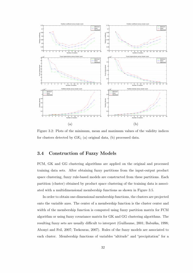
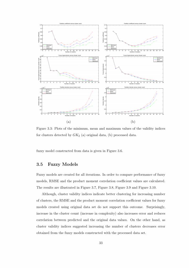


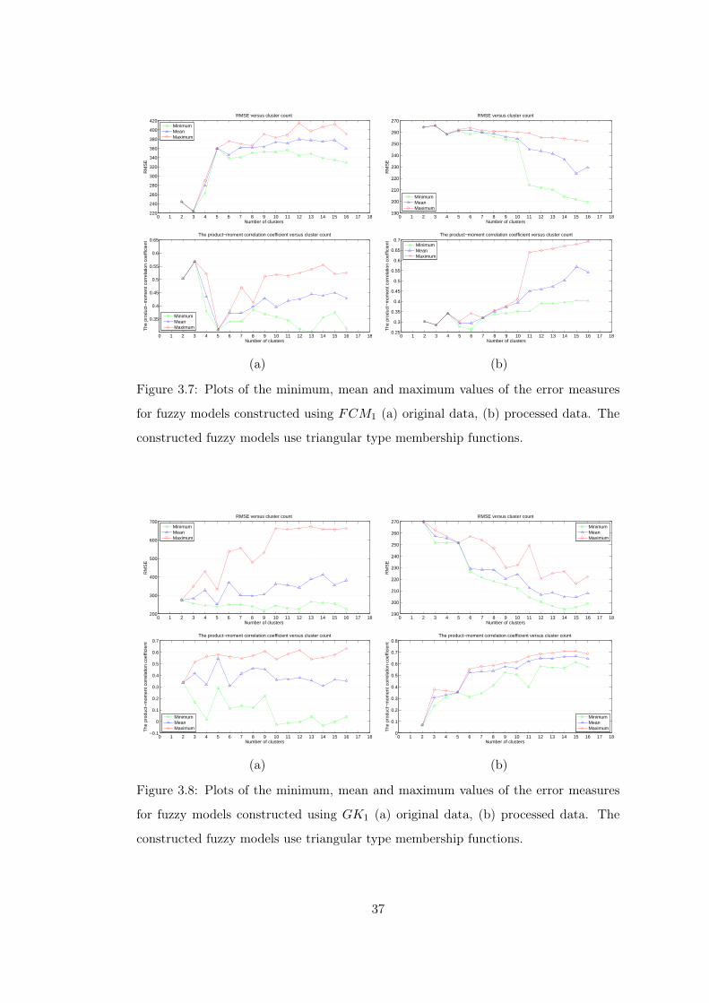


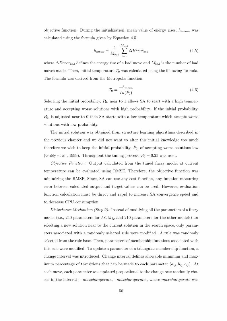


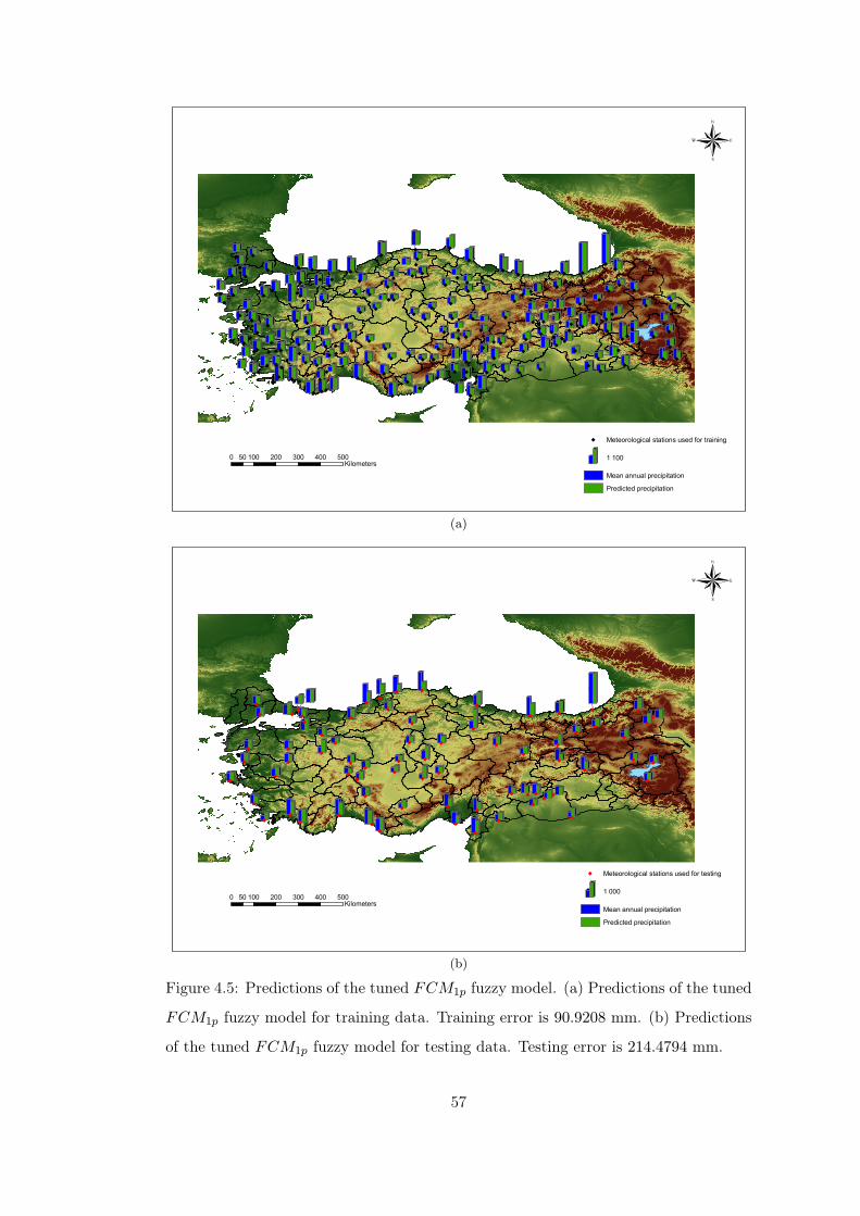
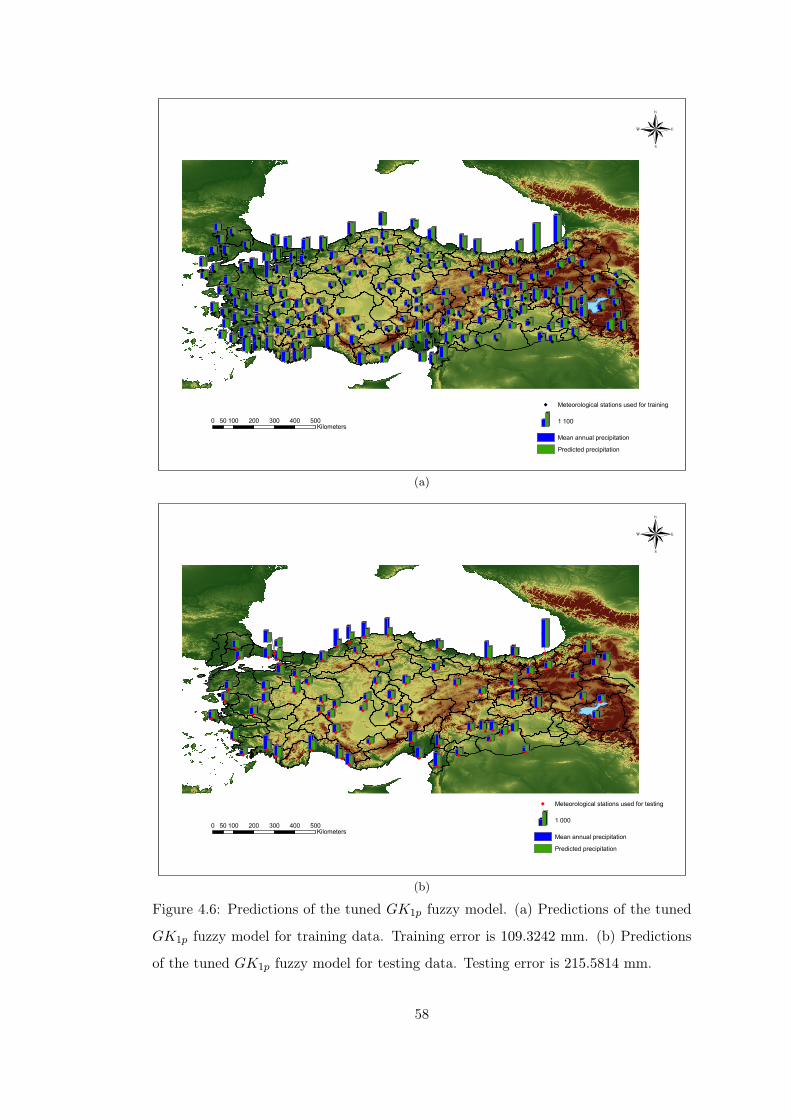


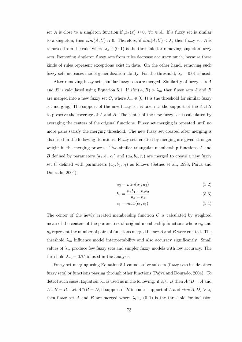


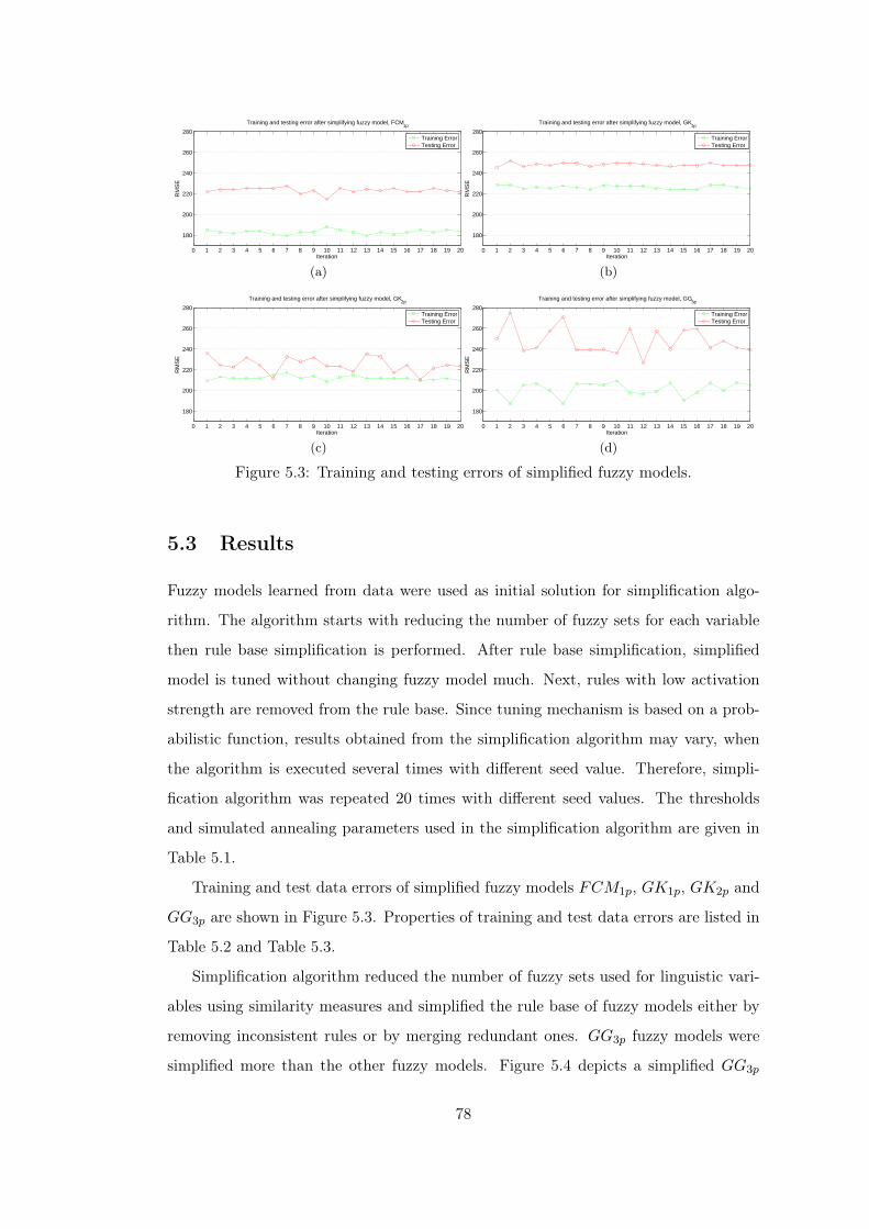


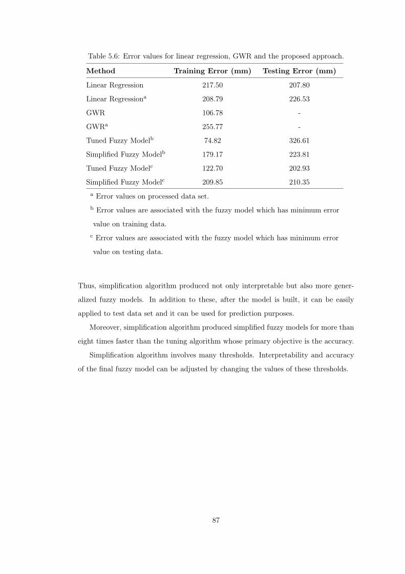


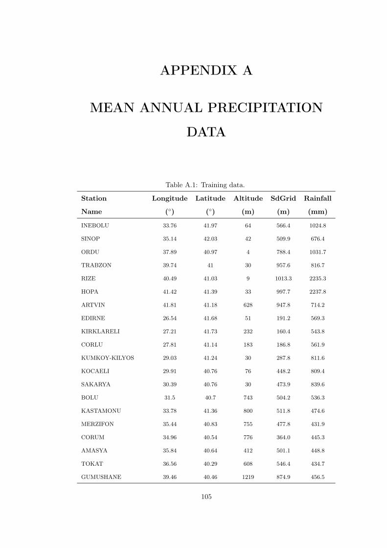

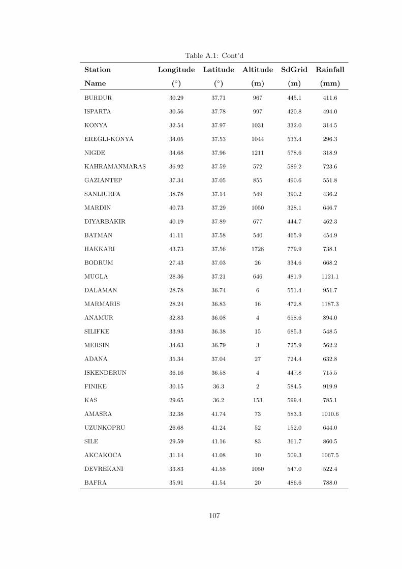

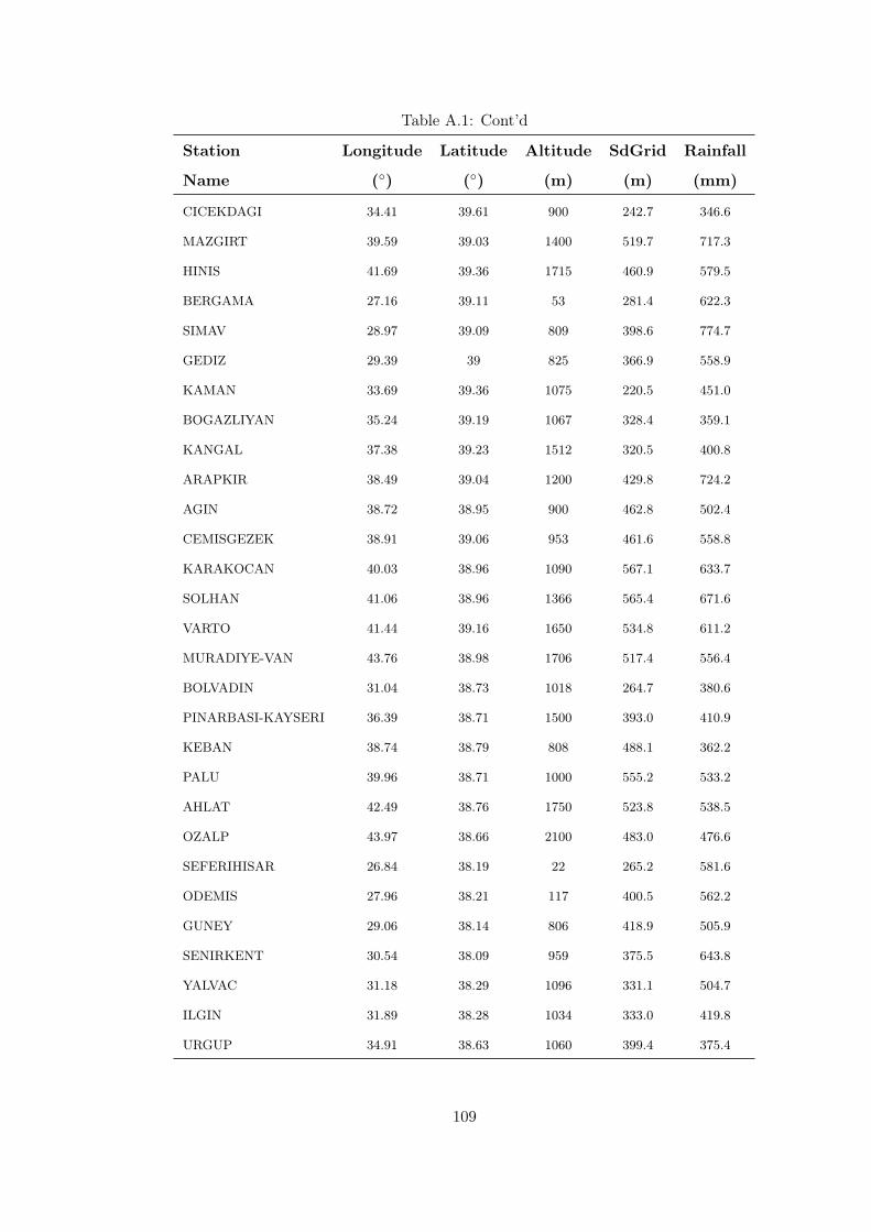
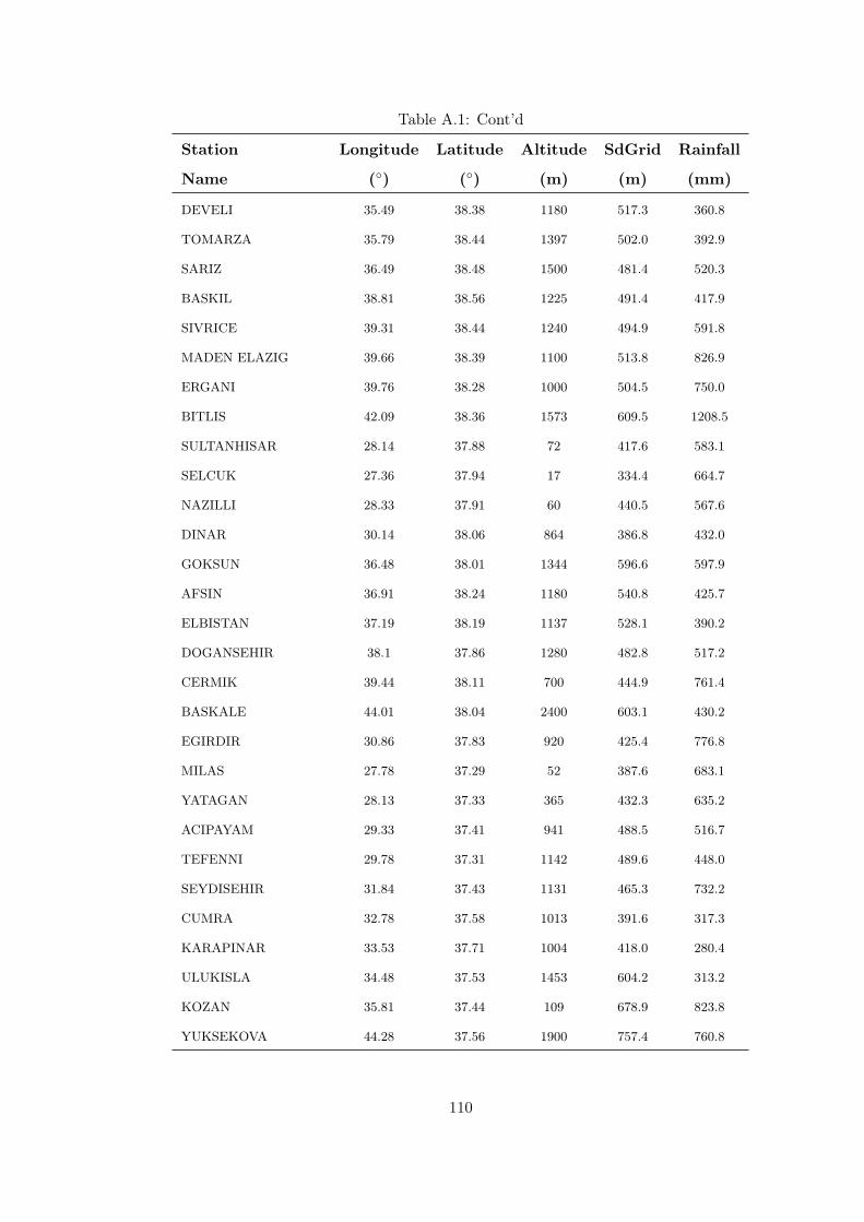


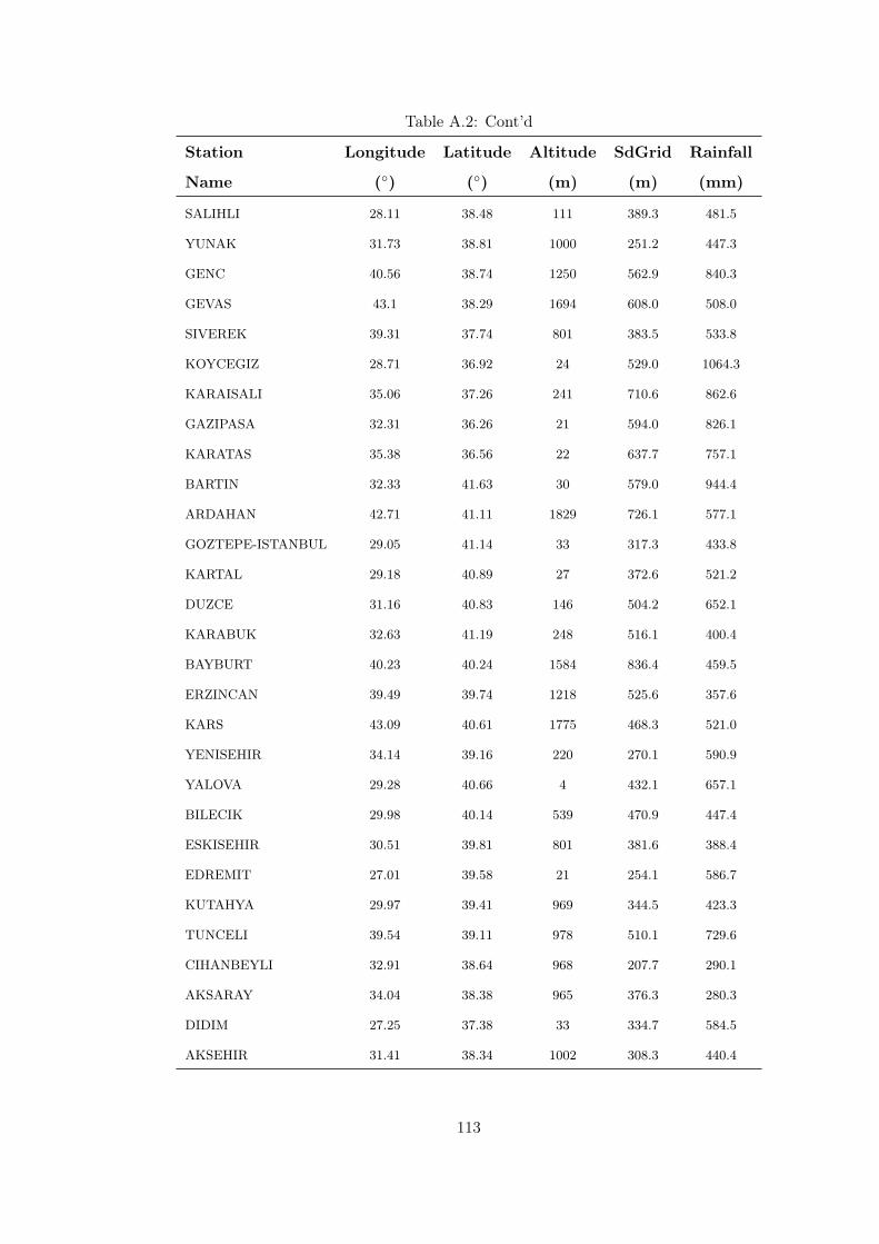


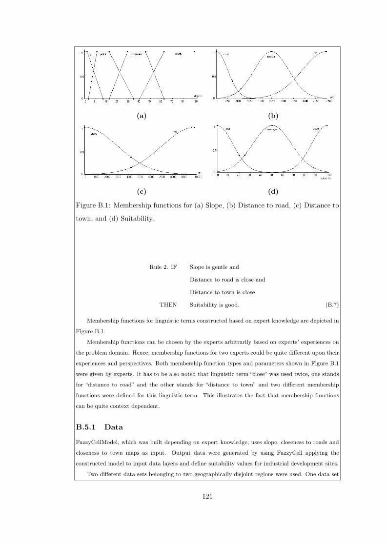


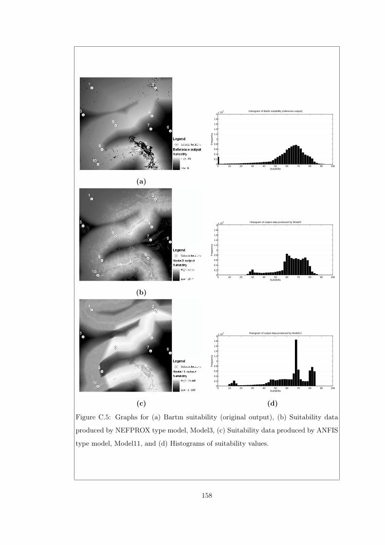


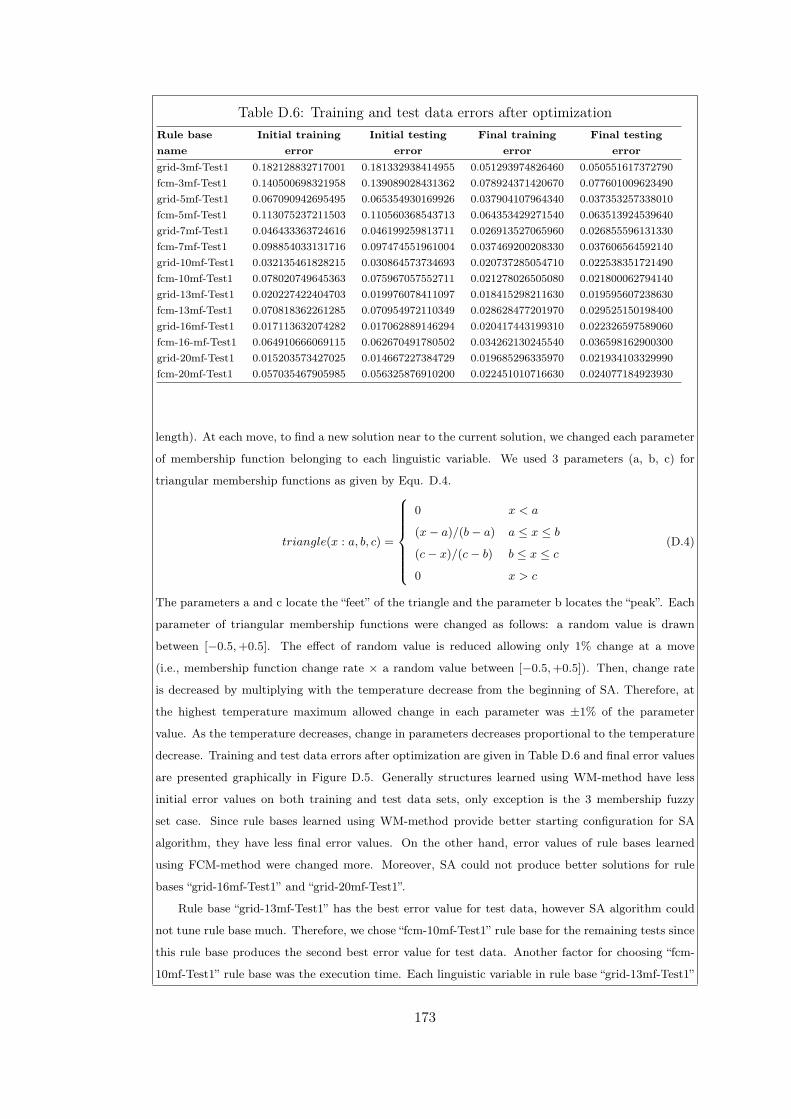
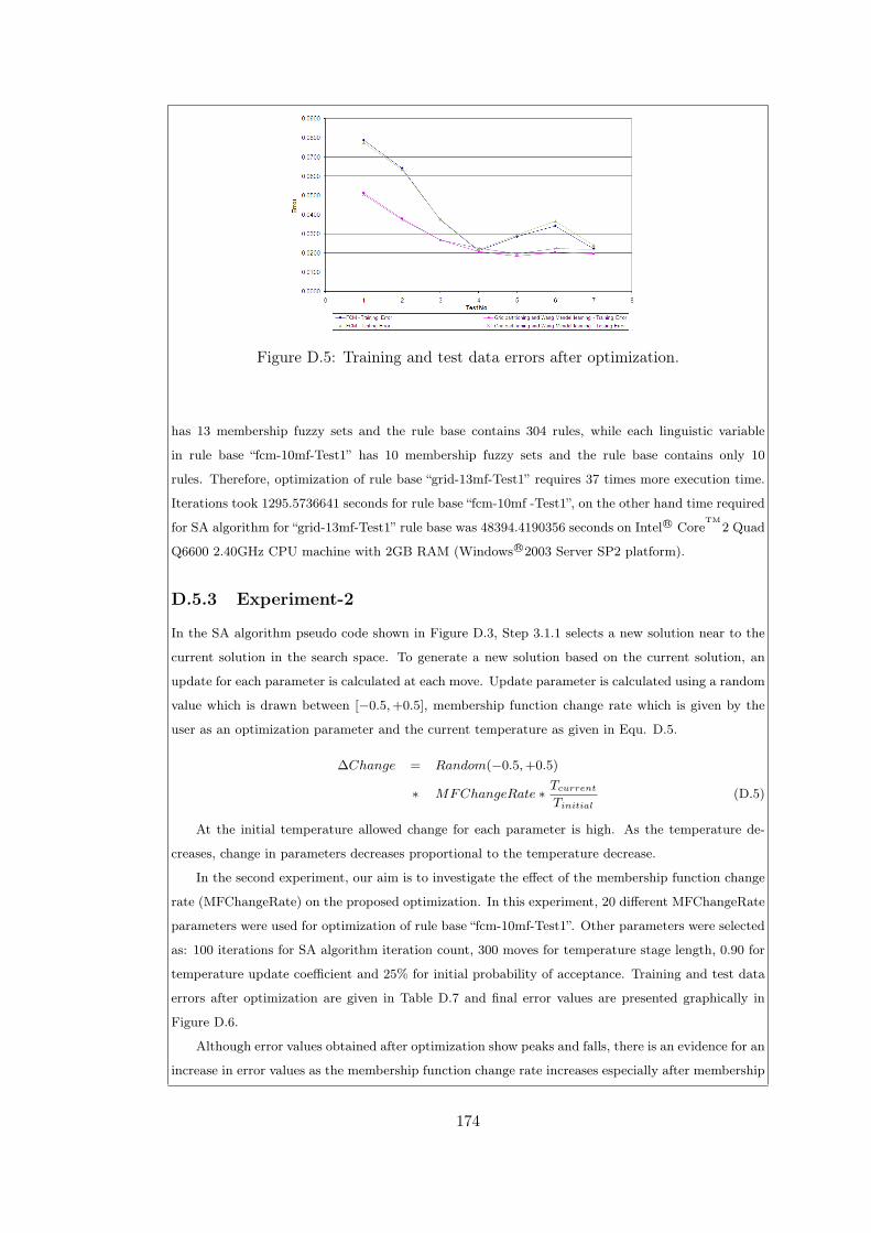


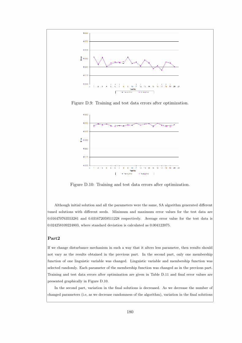


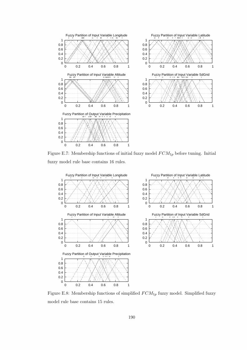


![Index [assets.cambridge.org]assets.cambridge.org/97811070/21259/index/9781107021259_index.pdfIndex ... Index](https://static.documents.pub/doc/80x56/5e6e9051865fe77870536fbb/-index-index-index.jpg)
![Bioassessment in complex environments: designing an index ......multimetric index [pMMI]) into a single index (the California Stream Condition Index [CSCI]). Evaluation of index performance](https://static.documents.pub/doc/80x56/6100690503752443811dbfcc/bioassessment-in-complex-environments-designing-an-index-multimetric-index.jpg)


![2 3 4 5 void ordered_fill (float* array, int array_length) { int index; for (index = 0; index < array_length; index++) { array[index] = index; }](https://static.documents.pub/doc/80x56/56649e0d5503460f94af6e07/2-3-4-5-void-orderedfill-float-array-int-arraylength-int-index-for.jpg)

