Laboratory Module 1 Indexing X-Ray Diffraction Patterns LEARNING OBJECTIVES Upon completion of this module you will be able to index an X-ray diffraction pattern, identify the Bravais lattice, and calculate the lattice parameters for crystalline materials. BACKGROUND We need to know about crystal structures because structure, to a large extent, determines properties. X-ray diffraction (XRD) is one of a number of experimental tools that are used to identify the structures of crystalline solids. The XRD patterns, the product of an XRD experiment, are somewhat like fingerprints in that they are unique to the material that is being examined. The information in an XRD pattern is a direct result of two things: (1) The size and shape of the unit cells determine the relative positions of the diffraction peaks; (2) Atomic positions within the unit cell determine the relative intensities of the diffraction peaks (remember the structure factor?). Taking these things into account, we can calculate the size and shape of a unit cell from the positions of the XRD peaks and we can determine the positions of the atoms in the unit cell from the intensities of the diffraction peaks. Full identification of crystal structures is a multi-step process that consists of: (1) Calculation of the size and shape of the unit cell from the XRD peak positions; (2) Computation of the number of atoms/unit cell from the size and shape of the cell, chemical composition, and measured density; (3) Determination of atom positions from the relative intensities of the XRD peaks We will only concern ourselves with step (1), calculation of the size and shape of the unit cell from XRD peak positions. We loosely refer to this as “indexing.” The laboratory module is broken down into two sections. The first addresses how to index patterns from cubic materials. The second addresses how to index patterns from non-cubic materials.
LEARNING OBJECTIVES Upon completion of this module you will be able to index an X-ray diffraction pattern, identify the Bravais lattice, and calculate the lattice parameters for crystalline materials.
BACKGROUND We need to know about crystal structures because structure, to a large extent, determines properties. X-ray diffraction (XRD) is one of a number of experimental tools that are used to identify the structures of crystalline solids. The XRD patterns, the product of an XRD experiment, are somewhat like fingerprints in that they are unique to the material that is being examined. The information in an XRD pattern is a direct result of two things:
(1) The size and shape of the unit cells determine the relative positions of the diffraction peaks;
(2) Atomic positions within the unit cell determine the relative intensities of the diffraction peaks (remember the structure factor?).
Taking these things into account, we can calculate the size and shape of a unit cell from the positions of the XRD peaks and we can determine the positions of the atoms in the unit cell from the intensities of the diffraction peaks. Full identification of crystal structures is a multi-step process that consists of:
(1) Calculation of the size and shape of the unit cell from the XRD peak positions; (2) Computation of the number of atoms/unit cell from the size and shape of the cell,
chemical composition, and measured density; (3) Determination of atom positions from the relative intensities of the XRD peaks
We will only concern ourselves with step (1), calculation of the size and shape of the unit cell from XRD peak positions. We loosely refer to this as “indexing.” The laboratory module is broken down into two sections. The first addresses how to index patterns from cubic materials. The second addresses how to index patterns from non-cubic materials.
PART 1 PROCEDURE FOR INDEXING CUBIC XRD PATTERNS
When you index a diffraction pattern, you assign the correct Miller indices to each peak (reflection) in the diffraction pattern. An XRD pattern is properly indexed when ALL of the peaks in the diffraction pattern are labeled and no peaks expected for the particular structure are missing.
This is an example of a properly indexed diffraction pattern. All peaks are accounted for. One now needs only to assign the correct Bravais lattice and to calculate lattice parameters. How to we correctly index a pattern? The correct procedures follow.
PROCEDURE FOR INDEXING AN XRD PATTERN The procedures are standard. They work for any crystal structure regardless of whether the material is a metal, a ceramic, a semiconductor, a zeolite, etc… There are two methods of analysis. You will do both. One I will refer to as the mathematical method. The second is known as the analytical method. The details are covered below.
Mathematical Method Interplanar spacings in cubic crystals can be written in terms of lattice parameters using the plane spacing equation:
2 2
2 2
1 h k ld a
2+ +=
You should recall Bragg’s law ( 2 sindλ θ= ), which can be re-written either as:
2 2 24 sindλ θ= OR 2
22sin
4dλθ =
Combining this relationship with the plane spacing equation gives us a new relationship:
2 2 2 2
2 2
1 4h k ld a 2
sin θλ
+ += = ,
which can be rearranged to:
( )2
2 22sin
4h k l
aλθ
⎛ ⎞= +⎜ ⎟
⎝ ⎠2 2+
The term in parentheses 2
24aλ⎛
⎜⎝ ⎠
⎞⎟ is constant for any one pattern (because the X-ray
wavelength λ and the lattice parameters a do not change). Thus 2sin θ is proportional to . This proportionality shows that planes with higher Miller indices will diffract
at higher values of θ.
2 2h k l+ + 2
Since 2
24aλ⎛
⎜⎝ ⎠
⎞⎟ is constant for any pattern, we can write the following relationship for any
two different planes:
( )
( )
22 2 2
1 1 1221
2 22 2 2 2
2 2 22
4sinsin
4
h k la
h k la
λθθ λ
⎛ ⎞+ +⎜ ⎟
⎝ ⎠=⎛ ⎞
+ +⎜ ⎟⎝ ⎠
or ( )( )
2 2 221 1 11
2 2 2 22 2 2 2
sinsin
h k l
h k lθθ
+ +=
+ +.
The ratio of 2sin θ values scales with the ratio of 2 2h k l 2+ + values. In cubic systems, the first XRD peak in the XRD pattern will be due to diffraction from planes with the lowest Miller indices, which interestingly enough are the close packed planes (i.e.: simple cubic, (100), 2 2h k l 2+ + =1; body-centered cubic, (110) =2; and face-centered cubic, (111) =3).
2 2h k l+ + 2
22 2h k l+ +
Since h, k, and l are always integers, we can obtain h k2 2 2l+ + values by dividing the 2sin θ values for the different XRD peaks with the minimum one in the pattern (i.e., the 2sin θ value from the first XRD peak) and multiplying that ratio by the proper integer
(either 1, 2 or 3). This should yield a list of integers that represent the various values. You can identify the correct Bravais lattice by recognizing the sequence of allowed reflections for cubic lattices (i.e., the sequence of allowed peaks written in terms of the quadratic form of the Miller indices).
2 2h k l+ + 2
2
2
2
2
Primitive = 1,2,3,4,5,6,8,9,10,11,12,13,14,16… 2 2h k l+ +Body-centered = 2,4,6,8,10,12,14,16… 2 2h k l+ +Face-centered = 3,4,8,11,12,16,19,20,24,27,32… 2 2h k l+ +Diamond cubic = 3,8,11,16,19,24,27,32… 2 2h k l+ + The lattice parameters can be calculated from:
( )2
2 22sin
4h k l
aλθ
⎛ ⎞= +⎜ ⎟
⎝ ⎠2 2+
which can be re-written as:
( )2
2 2 2 224sin
a h k lλθ
= + + 2 2 2
2sina h k lλ
θ= + + OR
Worked Example Consider the following XRD pattern for Aluminum, which was collected using CuKα radiation.
Index this pattern and determine the lattice parameters. Steps:
(1) Identify the peaks. (2) Determine 2sin θ . (3) Calculate the ratio 2sin θ / 2
minsin θ and multiply by the appropriate integers. (4) Select the result from (3) that yields 2 2h k l 2+ + as an integer. (5) Compare results with the sequences of 2 2h k l 2+ + values to identify the Bravais
lattice. (6) Calculate lattice parameters.
Here we go!
(1) Identify the peaks and their proper 2θ values. Eight peaks for this pattern. Note: most patterns will contain α1 and α2 peaks at higher angles. It is common to neglect α2 peaks.
Analytical Method This is an alternative approach that will yield the same results as the mathematical method. It will give you a nice comparison. Recall:
( )2
2 2 2 22sin
4h k l
aλθ
⎛ ⎞= + +⎜ ⎟
⎝ ⎠ and
2
2 = constant4aλ⎛ ⎞
⎜ ⎟⎝ ⎠
for all patterns
If we let K = 2
24aλ⎛ ⎞
⎜⎝ ⎠
⎟ , we can re-write these equations as:
( )2 2 2sin 2K h k lθ = + +
For any cubic system, the possible values of 2 2h k l 2+ + correspond to the sequence:
2 2h k l+ + 2 = 1,2,3,4,5,6,8,9,10,11… If we determine 2sin θ for each peak and we divide the values by the integers 2,3,4,5,6,8,9,10,11…, we can obtain a common quotient, which is the value of K corresponding to = 1. 2 2h k l+ + 2
K is related to the lattice parameter as follows:
2
24K
aλ⎛
= ⎜⎝ ⎠
⎞⎟ OR
2a
Kλ
=
If we divide the 2sin θ values for each reflection by K, we get the 2 2h k l 2+ + values. The sequence of values can be used to label each XRD peak and to identify the Bravais lattice.
2 2h k l+ + 2
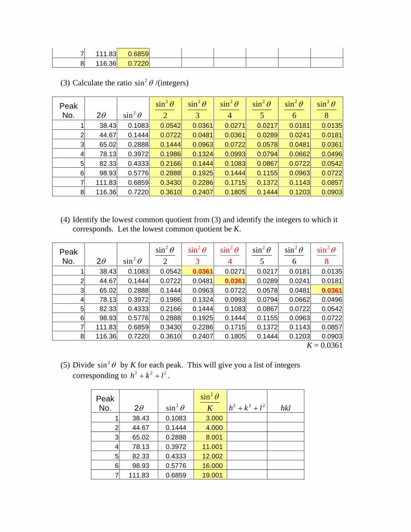
Let’s do an example for the Aluminum pattern presented above. Steps:
(1) Identify the peaks. (2) Determine 2sin θ . (3) Calculate the ratio 2sin θ /(integers) (4) Identify the lowest common quotient from (3) and identify the integers to which it
corresponds. Let the lowest common quotient be K. (5) Divide 2sin θ by K for each peak. This will give you a list of integers
corresponding to . 2 2h k l+ + 2
2(6) Select the appropriate pattern of 2 2h k l+ + values and identify the Bravais lattice. (7) Calculate lattice parameters.
Sequence suggests a Face-Centered Cubic Bravais Lattice
(7) Calculate lattice parameters.
1.540562 A2 2 0.0361
aK
λ= = = 4.0541 Å
These methods will work for any cubic material. This means metals, ceramics, ionic crystals, minerals, intermetallics, semiconductors, etc…
PART 2 PROCEDURE FOR INDEXING NON-CUBIC XRD PATTERNS
The procedures are standard and will work for any crystal. The equations will differ slightly from each other due to differences in crystal size and shape (i.e., crystal structure). As was the case for cubic crystals, there are two methods of analysis that involve calculations. You will do both. One I will refer to as the mathematical method. The second I will refer to as the analytical method. Both the mathematical and graphical methods require some knowledge of the crystal structure that you are dealing with and the resulting lattice parameter ratios (e.g., c/a, b/a, etc…). This information can be determined graphically using Hull-Davey charts. We will first introduce the concept of Hull-Davey charts prior to showing how to proper index patterns.
Hull-Davey Charts
The graphical method developed by Hull and Davey1 are convenient for indexing diffraction patterns, in particular for systems of lower symmetry. The reason is that this method allows one to determine structure even if lattice parameters are unknown. The mathematical methods that will be illustrated in later sections of this module require such knowledge, in particular the values of the various lattice parameter ratios (c/a, b/a, c/b etc…). The steps involved in constructing and indexing patterns using Hull-Davey charts is very straightforward. First, consider the plane spacing equations for the crystal structures of interest. Some examples are shown below:
Hexagonal 2 2
2 2
1 43
h hk k ld a
⎛ ⎞+ + 2
2c= +⎜ ⎟
⎝ ⎠
Tetragonal 2 2 2
2 2
1 h k ld a
+2c
= +
Orthorhombic 2 2
2 2 2
1 h k ld a b c
2
2= + +
Etc. You should recall Bragg’s law ( 2 sindλ θ= ), which can be re-written either as:
2 2 24 sindλ θ=
or
22
2sin4dλθ =
Combining Bragg’s law with the plane spacing equations yields the relationship:
Hexagonal 2 2 2
2 2 2
1 4 4sin3
h hk k ld a c
2
2
θλ
⎛ ⎞+ += + =⎜ ⎟
⎝ ⎠
Tetragonal 2 2 2 2
2 2 2 2
1 4h k ld a c
sin θλ
+= + =
Orthorhombic 2 2 2 2
2 2 2 2 2
1 4h k ld a b c
sin θλ
= + + =
Etc… which can be rearranged in terms of sin2θ to:
1 A.W. Hull and W.P. Davey, Phys. Rev., vol. 17, pp. 549, 1921; W.P. Davey, Gen. Elec. Rev., vol. 25, pp. 564, 1922.
Hexagonal 2 2 2
22 2
4sin4 3
h hk k la c
λθ2⎡ ⎤⎛ ⎞ ⎛ ⎞+ +
= = +⎢ ⎥⎜ ⎟ ⎜ ⎟⎝ ⎠ ⎝ ⎠⎣ ⎦
Tetragonal 2 2 2 2
22 2sin
4h k l
a cλθ
⎛ ⎞⎛ += +⎜ ⎟⎜
⎝ ⎠⎝
⎞⎟⎠
Orthorhombic 2 2 2 2
22 2 2sin
4h k la b c
λθ⎛ ⎞⎛
= + +⎜ ⎟⎜⎝ ⎠⎝
⎞⎟⎠
You should note that as unlike cubic systems where 2
24aλ⎛
⎜⎝ ⎠
⎞⎟ is constant, your results for
non-cubic systems will depend upon ratios of lattice parameters (i.e., c/a, b/a, etc.) and your interaxial angles (i.e., α, β, γ). We will illustrate this (“sort of”) below. This is due to the non-equivalence of indices in these systems (e.g., tetragonal – 001 ≠ 100; orthorhombic – 001 ≠ 010 ≠ 100; etc…). Let’s concentrate on hexagonal systems for the time being. I may ask you to derive relationships for tetragonal and orthorhombic systems in a homework assignment. As noted previously, the mathematical method requires knowledge of the c/a ratio. We don’t know what it is so we need to construct a Hull-Davey chart. To accomplish this goal, we must first rewrite our revised d-spacing equations as follows:
( )
2 2 2 2
2 2 2 2
22 2
2
1 4 4sin3
42log 2log log3 (
h hk k ld a c
ld a h hk kc a
θλ
⎛ ⎞+ += + =⎜ ⎟
⎝ ⎠⇓
/ )⎡ ⎤
= − + + +⎢ ⎥⎣ ⎦
Letting the term in brackets equal s, we finally end up with:
[ ]2log 2log logd a= − s
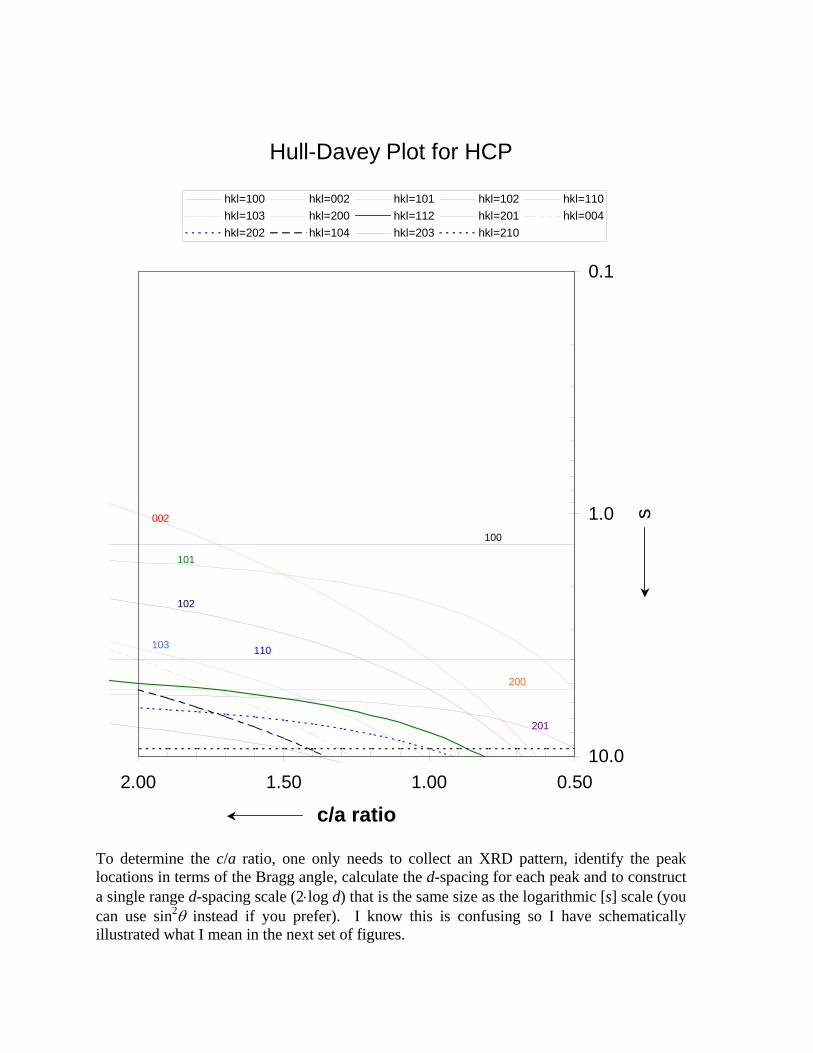
We can now construct the Hull-Davey chart by plotting the variation of log [s] with c/a for different hkl values. One axis will consist of c/a values while the other will consist of -log [s] values with the origin set at log [1] = 0. A representative chart is presented on the next page.
To determine the c/a ratio, one only needs to collect an XRD pattern, identify the peak locations in terms of the Bragg angle, calculate the d-spacing for each peak and to construct a single range d-spacing scale (2⋅log d) that is the same size as the logarithmic [s] scale (you can use sin2θ instead if you prefer). I know this is confusing so I have schematically illustrated what I mean in the next set of figures.
h1k1l1
h2k2l2
h3k3l3
h4k4l4
c/a ratio
log [s]
+
d scale
sin2θ-scale
1.0 1.0 1.0
+
Next, you need to calculate the d-spacing or sin2θ values for the observed peaks and mark them on a strip laid along side the appropriate d- or sin2θ - scale.
h1k1l1
h2k2l2
h3k3l3
h4k4l4
c/a ratio
log [s]
+
sin2θ-scale
d scale
1.0 1.0 1.0
+
The strip should be moved horizontally and vertically across the log [s] – c/a plot until a position is found where each mark on your strip coincides with a line on the chart. This is illustrated schematically on the next figure.
Please keep in mind that my illustrations for the Hull-Davey method are SCHEMATIC. This method is very difficult to convey. You should consult the classical references to find
out more information about this technique.
h1k1l1
h2k2l2
h3k3l3
h4k4l4
c/a ratio
log [s]
+
+
0.10
10.0
10.0
1.0
d scale
1.0 1.0
This is our c/a ratio for the pattern!
This method really does work as I showed you in class. Once you know your c/a ratio, you can index the XRD pattern. As we noted above, there are two ways to do this. The first is the mathematical method.
Mathematical Method for Non-Cubic Crystals Recall the following equation:
( )2 2
2 2 22 2
4sin4 3 ( / )
lh hk ka c
λθ⎛ ⎞ ⎡
= + + +⎜ ⎟ a⎤
⎢ ⎥⎝ ⎠ ⎣ ⎦
Note that the lattice parameter a and the ratio of lattice parameters c/a are constant for a
given diffraction pattern. Thus, 2
24aλ⎛
⎜⎝ ⎠
⎞⎟ is constant for any pattern. The pattern can now be
indexed in by considering the terms in brackets:
( )2 243
h hk k+ +
2
2( / )l
c a
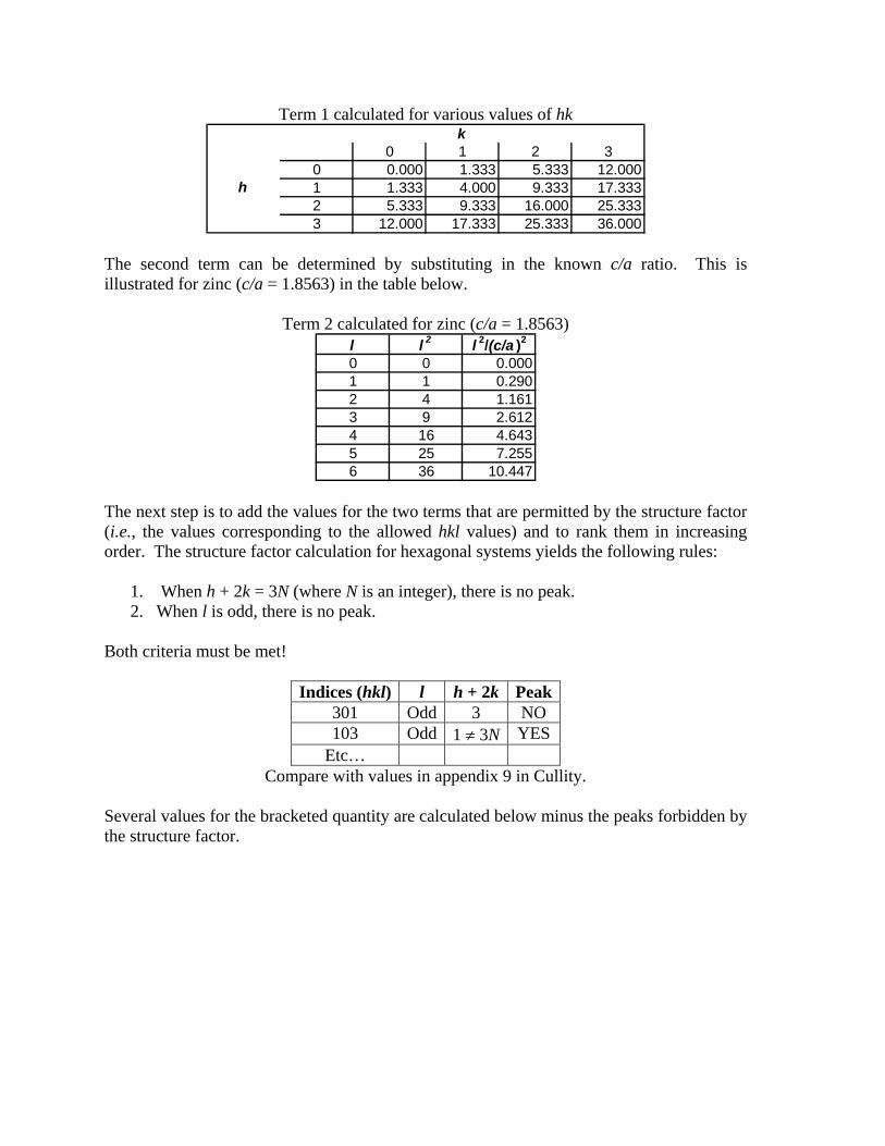
Let’s start with term 1. This term only depends on the indices h and k. Thus its value can be calculated for different values of h and k. This is done below for various hk values.
The next step is to add the values for the two terms that are permitted by the structure factor (i.e., the values corresponding to the allowed hkl values) and to rank them in increasing order. The structure factor calculation for hexagonal systems yields the following rules:
1. When h + 2k = 3N (where N is an integer), there is no peak. 2. When l is odd, there is no peak.
Both criteria must be met!
Indices (hkl) l h + 2k Peak301 Odd 3 NO 103 Odd 1 ≠ 3N YES
Etc… Compare with values in appendix 9 in Cullity.
Several values for the bracketed quantity are calculated below minus the peaks forbidden by the structure factor.
The values in this table have been calculated for specific (hkl) planes. We can assign specific hkl values for each of the peaks in a hexagonal unknown by noting that the sequence of peaks will be the same as indicated in the table. Lattice parameters can be determined in two ways: We can calculate a by looking for peaks where l = 0 (i.e., hk0 peaks). If you substitute l = 0 into:
( )2 2
2 2 22 2
4sin4 3 ( / )
lh hk ka c
λθ⎛ ⎞ ⎡
= + + +⎜ ⎟ a⎤
⎢ ⎥⎝ ⎠ ⎣ ⎦
you will get,
( )2
2 22
4sin4 3
h hk ka
λθ⎛ ⎞ 2⎡ ⎤= +⎜ ⎟ +⎢ ⎥⎣ ⎦⎝ ⎠
OR
2 2
3 sina h hk kλ
θ= + +
You can now perform this calculation for every hk0 peak, which will yield values for a. Similarly, values for c can be determined by looking for 00l type peaks. In these instances, h = k = 0. Thus,
( )2 2
2 2 22 2
4sin4 3 ( / )
lh hk ka c
λθ⎛ ⎞ ⎡
= + + +⎜ ⎟ a⎤
⎢ ⎥⎝ ⎠ ⎣ ⎦
becomes
2sinc lλ
θ=
Worked Example Consider the following XRD pattern for Titanium, which was collected using CuKα radiation.
20 30 40 50 60 70 80 90 100
Titanium Powder (-325 mesh)
Two Theta
Inte
nsity
(co
unts
)
CuKα radiation λ = 1.540562 Å
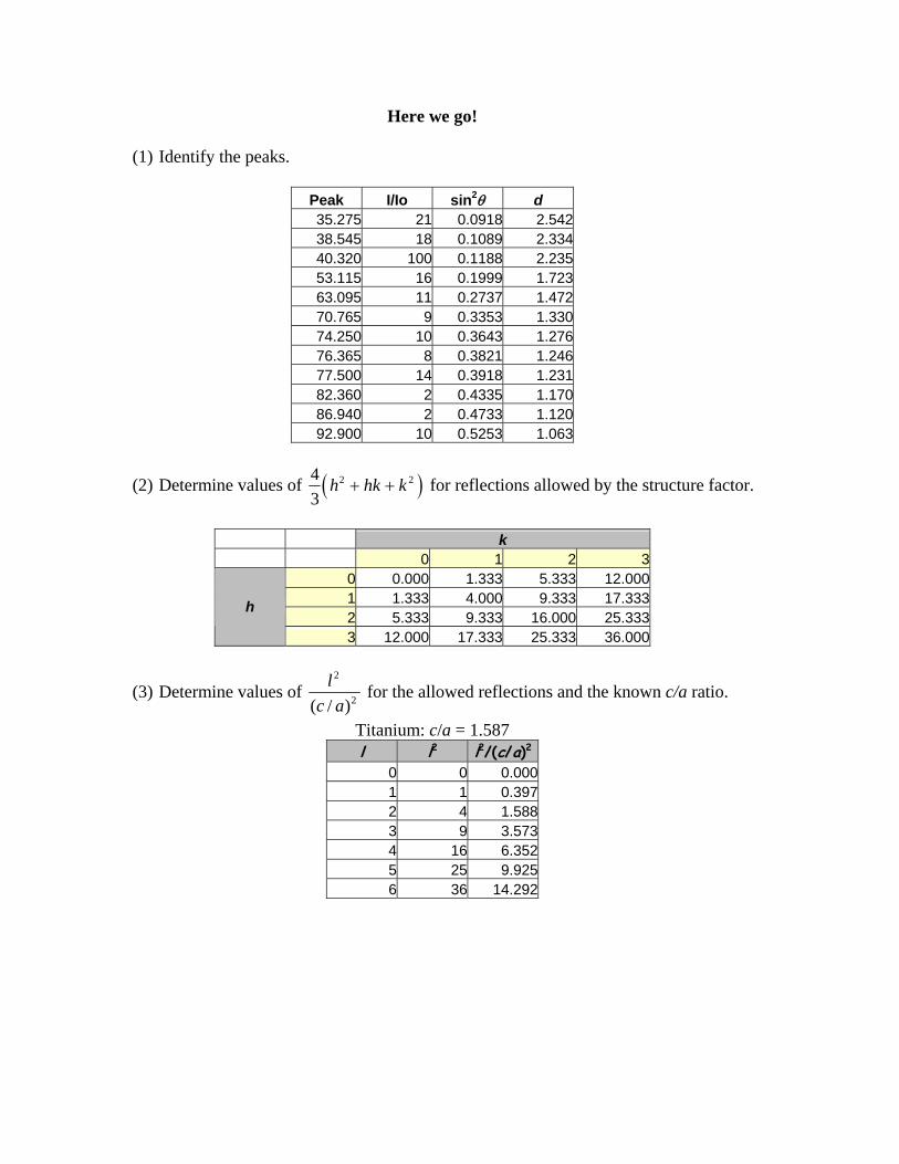
Index this pattern and determine the lattice parameters. Steps:
(1) Identify the peaks.
(2) Determine values of ( 243
h hk k+ + )2 for reflections allowed by the structure factor.
(3) Determine values of 2
2( / )l
c a for the allowed reflections and the known c/a ratio
(4) Add the solutions from parts (2) and (3) together and re-arrange them in increasing order.
(5) Use this order to assign indices to the peaks in your diffraction pattern. (6) Look for hk0 type reflections and calculate a for these reflections. (7) Look for 00l type reflections. Calculate c for these reflections.
Pretty good correlation with ICDD value. Actual c/a for Titanium is 1.5871 This method, though effective for most powder XRD data, can yield the wrong results if XRD peaks are missing from your XRD pattern. In other words, missing peaks can cause you to assign the wrong hkl values to a peak. Other methods should be available.
Analytical Method for Non-Cubic Crystals To accurately apply this technique, one must first consider our altered plane spacing equation:
( )2 2
2 2 22 2
4sin34 (
lh hk ka c
λθ⎛ ⎞ ⎡
= + + +⎜ ⎟ / )a⎤
⎢ ⎥⎝ ⎠ ⎣ ⎦
Since a and c/a are constants for any given pattern, we can re-arrange this equation to:
( )2 2 2sin A h hk k Clθ = + + + 2
where 2
23A
aλ
= and 2
24C
cλ
= . Since h, k, and l are always integers, the term in
parentheses, can only have values like 0, 1, 3, 4, 7, 9, 12… and l2h hk k+ + 2 2 can only have values like 0, 1, 4, 9,…. We need to calculate 2sin θ for each peak, divide each 2sin θ value by the integers 3, 4, 7, 9… and look for the common quotient (i.e., the 2sin / nθ value that is equal to one of the observed 2sin θ values). The 2sin θ values representing this common quotient refer to hk0 type peaks. Thus this common quotient can be tentatively assigned as A. We can now re-arrange terms in our modified equation to obtain C. This is done as follows:
( )
( )
2 2 2
2 2 2
sin
sin
2
2
A h hk k Cl
Cl A h hk k
θ
θ
= + + +
⇓
= − + +
We get the value of C by subtracting from each 2sin θ the values of n⋅A (i.e., A, 3A, 4A, 7A,…) where A is the common quotient that we identified above. Next, we need to look for the remainders that are in the ratio of 1, 4, 9, 16…, which will be peaks of the 00l type. We can determine C from these peaks. The remaining peaks are neither hk0-type nor 00l type. Instead they are hkl-type. They can be indexed from a combination of A and C values. Let’s do an example. Worked Example Steps:
(1) Identify the peaks and calculate 2sin θ for each peak. (2) Divide each 2sin θ value by the integers 3, 4, 7, 9…. (3) Look for the common quotient. (4) Let the lowest common quotient represent A. (5) Assign hk0 type indices to peaks. (6) Calculate 2sin θ - nA where n = 1, 3, 4, 7….
(7) Look for the lowest common quotient. From this we can identify 00l type peaks. Recall, that 001 is not allowed for hexagonal systems. The first 00l type peak will be 002. We can calculate C from:
2 2 2 2sin ( )C l A h hk kθ⋅ = − ⋅ + +
2in
(8) Look for values of s θ that increase by factors of 4, 9… (this is because l = 1, 2, 3… and l2 = 1, 4, 9…). Peaks exhibiting these characteristics are 00l type peaks, which can be assigned the indices 004, 009, etc…). Also note that the values of
2sin θ will be some integral number times the value observed in (7) which indicates the indices of the peak
(9) Peaks that are neither hk0 nor 00l can be identified using combinations of our calculated A and C values.
(10) Calculate the lattice parameters from the values of A and C.
Confused yet? You could be. I was the first time I learned these things. Let me show you an example that should make all things clear.
Here we go! Consider the diffraction pattern for Titanium as shown below. This one is a little different than the specimen that we analyzed above. Intensity (%)
Steps to success:1. Calculate sin2θ for each peak2. Divide each sin2θ value by integers 3, 4, 7… (from h2+hk+k2 allowed by the structure factor)3. Look for lowest common quotient.4. Let lowest common quotient = A .5. Peaks with lowest common quotient are hk 0 type peaks. Assign allowed hk 0 indices to peaks.
6. Subtract from each sin2θ value 3A , 4A , 7A … (from h 2+hk +k 2 allowed by the structure factor)
7. Look for lowest common quotient (LCQ). From this you can identify 00l -type peaks. The first allowed peak for hexagonal systems is 002. Determine C from the equation: C ⋅ l 2 = sin2θ-A (h 2+hk +k 2) since h =0 and k =0, then: C=LCQ/l 2 = sin2θ/l 2
8. Look for values of sin2θ that increase by factors of 4, 9, 16... (because l = 1,2,3,4..., l 2=1,4,9,16...) The peaks exhibiting these characteristics are 00l -type peaks (002...).
We identify the 4th peak as 102 because we observe the LCQ for sin2θ-1A. Recall that the 1 comes from the quadratic form of Miller indices (i.e., h 2+hk +k 2=1).
We identify the 8th peak as 112 because we observe the LCQ for sin2θ-3A. Recall that the 1 comes from the quadratic form of Miller indices (i.e., h 2+hk +k 2=3).
HOW DO THESE VALUES COMPARE WITH THOSE FROM THE ICDD CARDS?
9. Peaks that are not hk 0 or 00l can be identified using combinations of A and C values. This is accomplished by considering: sin2θ = C ⋅l 2 + A (h 2+hk +k 2) Cycle through allowed values for l and hk , and compare sin2θ value to labeled peaks.
10. Once A and C are known, the lattice parameters can be calculated.
sin2θ = C ⋅l 2 + A ⋅ (h 2+hk +k 2)
10. Once A and C are known, the lattice parameters can be calculated.