STATE OF INDIANA INDIANA UTILITY REGULATORY COMMISSION PETITION OF INDIANAPOLIS POWER & LIGHT COMPANY ("IPL") FOR AUTHORITY TO INCREASE RATES AND CHARGES FOR ELECTRIC UTILITY SERVICE AND FOR APPROVAL OF: (1) ACCOUNTING RELIEF, INCLUDING IMPLEMENTATION OF MAJOR STORM DAMAGE RESTORATION RESERVE ACCOUNT; (2) REVISED DEPRECIATION RATES; (3) THE INCLUSION IN BASIC RATES AND CHARGES OF THE COSTS OF CERTAIN PREVIOUSLY APPROVED QUALIFIED POLLUTION CONTROL PROPERTY; (4) IMPLEMENTATION OF NEW OR MODIFIED RATE ADJUSTMENT MECHANISMS TO TIMELY RECOGNIZE FOR RATEMAKING PURPOSES LOST REVENUES FROM DEMAND- SIDE MANAGEMENT PROGRAMS AND CHANGES IN (A) CAPACITY PURCHASE COSTS; (B) REGIONAL TRANSMISSION ORGANIZATION COSTS; AND (C) OFF SYSTEM SALES MARGINS; AND (5) NEW SCHEDULES OF RATES, RULES ANDREGULATIONS FOR SERVICE. ) ) ) ) ) ) ) ) ) ) ) ) ) ) ) ) ) CAUSE NO. 44576 IN THE MATTER OF THE INDIANA UTILITY REGULATORY COMMISSION'S INVESTIGATION INTO INDIANAPOLIS POWER & LIGHT COMPANY'S ONGOING INVESTMENT IN, AND OPERATION AND MAINTENANCE OF, ITS NETWORK FACILITIES ) ) ) ) ) CAUSE NO. 44602 VERIFIED DIRECT TESTIMONY OF GLENN A. WATKINS – PUBLIC’S EXHIBIT NO. 14 ON BEHALF OF THE INDIANA OFFICE OF UTILITY CONSUMER COUNSELOR JULY 27, 2015
Transcript
STATE OF INDIANA
INDIANA UTILITY REGULATORY COMMISSION PETITION OF INDIANAPOLIS POWER & LIGHT COMPANY ("IPL") FOR AUTHORITY TO INCREASE RATES AND CHARGES FOR ELECTRIC UTILITY SERVICE AND FOR APPROVAL OF: (1) ACCOUNTING RELIEF, INCLUDING IMPLEMENTATION OF MAJOR STORM DAMAGE RESTORATION RESERVE ACCOUNT; (2) REVISED DEPRECIATION RATES; (3) THE INCLUSION IN BASIC RATES AND CHARGES OF THE COSTS OF CERTAIN PREVIOUSLY APPROVED QUALIFIED POLLUTION CONTROL PROPERTY; (4) IMPLEMENTATION OF NEW OR MODIFIED RATE ADJUSTMENT MECHANISMS TO TIMELY RECOGNIZE FOR RATEMAKING PURPOSES LOST REVENUES FROM DEMAND-SIDE MANAGEMENT PROGRAMS AND CHANGES IN (A) CAPACITY PURCHASE COSTS; (B) REGIONAL TRANSMISSION ORGANIZATION COSTS; AND (C) OFF SYSTEM SALES MARGINS; AND (5) NEW SCHEDULES OF RATES, RULES ANDREGULATIONS FOR SERVICE.
)))))))))))))))))
CAUSE NO. 44576
IN THE MATTER OF THE INDIANA UTILITY REGULATORY COMMISSION'S INVESTIGATION INTO INDIANAPOLIS POWER & LIGHT COMPANY'S ONGOING INVESTMENT IN, AND OPERATION AND MAINTENANCE OF, ITS NETWORK FACILITIES
)))))
CAUSE NO. 44602
VERIFIED DIRECT TESTIMONY
OF
GLENN A. WATKINS – PUBLIC’S EXHIBIT NO. 14
ON BEHALF OF THE
INDIANA OFFICE OF UTILITY CONSUMER COUNSELOR
JULY 27, 2015
TABLE OF CONTENTS
PAGE
I. INTRODUCTION..............................................................................................................1 II. CLASS COST OF SERVICE ...........................................................................................2
A. Generation Plant ....................................................................................................6 1. Probability of Dispatch Method .............................................................15 2. Base-Intermediate Peak (“BIP”) Method ..............................................18 3. Peak & Average (“P&A”) Method .........................................................20
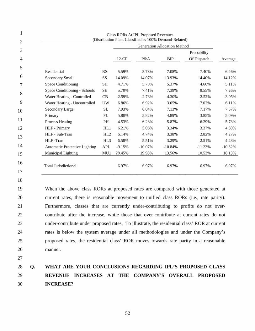
B. Transmission Plant ..............................................................................................24
C. Distribution Plant.................................................................................................25
III. IPL PROPOSED MIGRATION ADJUSTMENT ........................................................45 IV. CLASS REVENUE DISTRIBUTION ...........................................................................48 V. RATE DESIGN ................................................................................................................53
A. Residential Service ...............................................................................................53 1. Customer Charges ...................................................................................54 2. Declining-Block Rate Structure ..............................................................64
B. Water Heating (Rate Schedules CW and UW) .................................................68
C. Small Commercial Rate Design ..........................................................................69
D. Large Commercial/Industrial Rate Design .......................................................70 E. Interruptible Credit .............................................................................................70
1
VERIFIED DIRECT TESTIMONY OF GLENN A. WATKINS 1 ON BEHALF OF 2
INDIANA OFFICE OF UTILITY CONSUMER COUNSELOR 3 4 5
I. INTRODUCTION 6
7
Q. PLEASE STATE YOUR NAME AND BUSINESS ADDRESS. 8
A. My name is Glenn A. Watkins. My business address is 9030 Stony Point Parkway, Suite 9
580, Richmond, Virginia 23235. 10
11
Q. WHAT IS YOUR PROFESSIONAL AND EDUCATIONAL BACKGROUND? 12
A. I am a Principal and Senior Economist with Technical Associates, Inc., which is an 13
economics and financial consulting firm with an office in Richmond, Virginia. Except 14
for a six month period during 1987 in which I was employed by Old Dominion Electric 15
Cooperative, as its forecasting and rate economist, I have been employed by Technical 16
Associates continuously since 1980. 17
18
During my 34-year career at Technical Associates, I have conducted hundreds of 19
marginal and embedded cost of service, rate design, cost of capital, revenue requirement, 20
and load forecasting studies involving electric, gas, water/wastewater, and telephone 21
utilities throughout the United States and Canada and have provided expert testimony in 22
Massachusetts, Michigan, New Jersey, North Carolina, Ohio, Pennsylvania, Vermont, 24
Virginia, South Carolina, Washington, and West Virginia. In addition, I have provided 25
expert testimony before State and Federal courts as well as before State legislatures. A 26
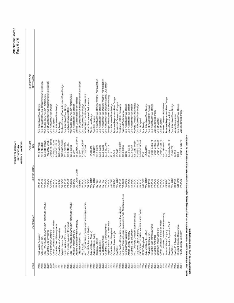
more complete description of my education and experience is provided in Attachment 27
GAW-1. 28
29
Q. WHAT IS THE PURPOSE OF YOUR TESTIMONY IN THIS PROCEEDING? 30
A. Technical Associates has been retained by the Indiana Office of Utility Consumer 31
Counselor (“OUCC”) to assist in its evaluation of the accuracy and reasonableness of 32
Indianapolis Power & Light Company’s (“IPL” or “Company”) retail class cost of service 33
2
study, proposed distribution of revenues by class, rate design, and other tariff issues. The 1
purpose of my testimony, therefore, is to comment on IPL’s proposals on these issues and 2
to present my findings and recommendations based on the results of the studies I have 3
undertaken on behalf of the OUCC. 4
5
II. CLASS COST OF SERVICE 6
7
Q. PLEASE BRIEFLY EXPLAIN THE CONCEPT OF A CLASS COST OF 8
SERVICE STUDY (“CCOSS”) AND ITS PURPOSE IN A RATE PROCEEDING. 9
A. Generally, there are two types of cost of service studies used in public utility ratemaking: 10
marginal cost studies and embedded, or fully allocated, cost studies. Consistent with the 11
practices of the Indiana Utility Regulatory Commission (“Commission”), IPL has 12
utilized a traditional embedded cost of service study for purposes of establishing the 13
overall revenue requirement in this case, as well as for class cost of service purposes. 14
15
Embedded class cost of service studies are also referred to as fully allocated cost studies 16
because the majority of a public utility’s plant investment and expense is incurred to 17
serve all customers in a joint manner. Accordingly, most costs cannot be specifically 18
attributed to a particular customer or group of customers. To the extent that certain costs 19
can be specifically attributed to a particular customer or group of customers, these costs 20
are directly assigned to that customer or group in the CCOSS. Since most of the utility’s 21
costs of providing service are jointly incurred to serve all or most customers, they must 22
be allocated across specific customers or customer rate classes. 23
24
It is generally accepted that to the extent possible, joint costs should be allocated to 25
customer classes based on the concept of cost causation. That is, costs are allocated to 26
customer classes based on analyses that measure the causes of the incurrence of costs to 27
the utility. Although the cost analyst strives to abide by this concept to the greatest 28
extent practical, some categories of costs, such as corporate overhead costs, cannot be 29
attributed to specific exogenous measures or factors, and must be subjectively assigned 30
or allocated to customer rate classes. With regard to those costs in which cost causation 31
3
can be attributed, there is often disagreement among cost of service experts on what is an 1
appropriate cost causation measure or factor; e.g., peak demand, energy usage, number of 2
customers, etc. 3
4
Q. IN YOUR OPINION, HOW SHOULD THE RESULTS OF A CCOSS BE 5
UTILIZED IN THE RATEMAKING PROCESS? 6
A. Although there are certain principles used by all cost of service analysts, there are often 7
significant disagreements on the specific factors that drive individual costs. These 8
disagreements can and do arise as a result of the quality of data and level of detail 9
available from financial records. There are also fundamental differences in opinions 10
regarding the cost causation factors that should be considered to properly allocate costs 11
to rate schedules or customer classes. Furthermore, and as mentioned previously, 12
numerous subjective decisions are required to allocate the myriad of jointly incurred 13
costs. 14
15
In these regards, two different cost studies conducted for the same utility and time period 16
can, and often do, yield different results. As such, regulators should consider CCOSS 17
only as a guide, with the results being used as one of many tools to assign class revenue 18
responsibility when cost causation factors cannot be realistically ascribed to some costs. 19
20
Q. HAVE THE HIGHER COURTS OPINED ON THE USEFULNESS OF COST 21
ALLOCATIONS FOR PURPOSES OF ESTABLISHING REVENUE 22
RESPONSIBILITY AND RATES? 23
A. Yes. In an important regulatory case involving Colorado Interstate Gas Company and 24
the Federal Power Commission (predecessor to FERC), the United States Supreme Court 25
stated: 26
But where as here several classes of services have a common use of the 27 same property, difficulties of separation are obvious. Allocation of costs 28 is not a matter for the slide-rule. It involves judgment on a myriad of 29 facts. It has no claim to an exact science.1 30
31
1 324 U.S. 581, 65 S. Ct. 829.
4
Q. DOES YOUR OPINION, AND THE FINDINGS OF THE U.S. SUPREME 1
COURT, IMPLY THAT COST ALLOCATIONS SHOULD PLAY NO ROLE IN 2
THE RATEMAKING PROCESS? 3
A. Not at all. It simply means that regulators should consider the fact that cost allocation 4
results are not surgically precise and that alternative, yet equally defensible approaches 5
may produce significantly different results. In this regard, when all reasonable cost 6
allocation approaches consistently show that certain classes are over or under 7
contributing to costs and/or profits, there is a strong rationale for assigning smaller or 8
greater percentage rate increases to these classes. On the other hand, if one set of 9
reasonable cost allocation approaches show dramatically different results than another 10
reasonable approach, caution should be exercised in assigning disproportionately larger 11
or smaller percentage increases to the classes in question. 12
13
Q. PLEASE EXPLAIN HOW YOU PROCEEDED WITH YOUR ANALYSIS OF 14
IPL’S CCOSS. 15
A. In conducting my independent analysis, I reviewed the structure and organization of the 16
Company’s CCOSS and reviewed the accuracy and completeness of the primary drivers 17
(allocators) used to assign costs to rate schedules and classes. Next, I reviewed IPL’s 18
selection of allocators to specific rate base, revenue, and expense accounts. I then 19
verified the accuracy of IPL’s CCOSS model by replicating its results using my own 20
computer model. Finally, I adjusted certain aspects of the Company’s study to better 21
reflect cost causation and cost incidence by rate schedule and customer class. It should 22
be noted that I originally completed my analyses based on the Company’s original filing. 23
On May 4, 2015, the Company filed its Fifth Revisions To Direct Testimony which 24
revised the testimony of Company witness Stephen Gaske. As a result of Mr. Gaske’s 25
revisions, I then incorporated his changes in my analyses such that my testimony and 26
schedules reflect Mr. Gaske’s May 4, 2015 revisions to his class cost of service study and 27
revenue distribution. 28
29
5
Q. NOTWITHSTANDING ANY CONCEPTUAL DISAGREEMENTS ON HOW 1
INDIVIDUAL COSTS SHOULD BE ALLOCATED ACROSS CLASSES, DID 2
YOU FIND THE COMPANY’S STUDY TO BE ACCURATE? 3
A. From an arithmetic perspective, I discovered what appears to be one minor error in the 4
CCOSS study sponsored by IPL witness Dr. Gaske. 5
6
Q. PLEASE DISCUSS THE MINOR ERROR YOU DISCOVERED WITHIN DR. 7
GASKE’S CCOSS. 8
A. This error relates only to the lighting classes and has no impact on other classes within 9
the CCOSS. IPL has two lighting rate classes: Automatic Protective Lighting (“APL”); 10
and, Municipal Lighting (“MU”). Dr. Gaske’s CCOSS utilizes current rate revenues of 11
$5,943,255 for rate APL and $10,747,745 for rate MU. However, his detailed revenue 12
proof indicates that APL’s rate revenues are $6,428,908 while MU’s rate revenues are 13
$10,262,445. It should be noted that these differences equally offset each other such that 14
the total lighting rate revenues are the same in both his CCOSS and revenue proof. 15
Furthermore, this correction does not impact any other rate class’ CCOSS results and has 16
no material impact on Dr. Gaske’s CCOSS findings as it relates to the two lighting rate 17
classes. A comparison of Dr. Gaske’s lighting rates of return to those corrected to 18
comport with his revenue proof is shown below: 19
20
21
22
23
24
25
Q. ARE THERE CERTAIN ASPECTS OF ELECTRIC UTILITY EMBEDDED 26
CCOSS THAT TEND TO BE MORE CONTROVERSIAL THAN OTHERS? 27
A. Yes. For decades, cost allocation experts and to some degree, utility commissions, have 28
disagreed on how generation and certain distribution plant accounts should be allocated 29
across classes. Beyond a doubt, these two issue areas are the most contentious and often 30
have the largest impact on the results of achieved class rates of return (“ROR”). 31
Rates of Return at Current Rates Rate IPL IPL Class As-Filed Study Corrected
APL -15.64% -12.28% MU 34.30% 29.89%
6
A. Generation Plant 1
2
Q. BEFORE I DISCUSS SPECIFIC COST ALLOCATION METHODOLOGIES, 3
PLEASE EXPLAIN HOW GENERATION/PRODUCTION-RELATED COSTS 4
ARE INCURRED; I.E., PLEASE EXPLAIN THE COST CAUSATION 5
CONCEPTS RELATING TO GENERATION/PRODUCTION RESOURCES. 6
A. Utilities design and build generation facilities to meet the energy and demand 7
requirements of their customers on a collective basis. Because of this, and the physical 8
laws of electricity, it is impossible to determine which customers are being served by 9
which facilities. As such, production facilities are joint costs; i.e., used by all customers. 10
Because of this commonality, production-related costs are not directly known for any 11
customer or customer group and must somehow be allocated. 12
13
If all customer classes used electricity at a constant rate (load) throughout the year, there 14
would be no disagreement as to the proper assignment of generation-related costs. All 15
analysts would agree that energy usage in terms of kilowatt-hour (“kWh”) would be the 16
proper approach to reflect cost causation and cost incidence. However, such is not the 17
case in that IPL experiences periods (hours) of much higher demand during certain times 18
of the year and across various hours of the day. Moreover, all customer classes do not 19
contribute in equal proportions to these varying demands placed on the generation 20
system. To further complicate matters the electric utility industry is unique in that there 21
is a distinct energy/capacity trade-off relating to production costs. That is, utilities design 22
their mix of production facilities (generation and power supply) to minimize the total 23
costs of energy and capacity, while also ensuring there is enough available capacity to 24
meet peak demands. The trade-off occurs between the level of fixed investment per unit 25
of capacity kilowatt (“kW”) and the variable cost of producing a unit of output (kWh). 26
Coal and nuclear units require high capital expenditures resulting in large investment per 27
kW, whereas smaller units with higher variable production costs generally require 28
significantly less investment per kW. Due to varying levels of demand placed on the 29
system over the course of each day, month, and year there is a unique optimal mix of 30
7
production facilities for each utility that minimizes the total cost of capacity and energy; 1
i.e., its cost of service. 2
3
Therefore, as a result of the energy/capacity cost trade-off, and the fact that the service 4
requirements of each utility are unique, many different allocation methodologies have 5
evolved in an attempt to equitably allocate joint production costs to individual classes. 6
7
Q. PLEASE EXPLAIN. 8
A. Total production costs vary each hour of the year. Theoretically, energy and capacity 9
costs should be allocated to customer classes each and every hour of the year. This 10
would result in 8,760 hourly allocations. Although such an analysis is certainly possible 11
with today’s technology, hourly supply (generation) and demand (customer load) data is 12
required to conduct such hour-by-hour analyses. While most utilities can and do record 13
hourly production output, they often do not estimate class loads on an hourly basis (at 14
least not for every hour of the year). With these constraints in mind, several allocation 15
methodologies have been developed to allocate electric utility generation plant 16
investment and attendant costs. Each of these methods has strengths and weaknesses 17
regarding the reasonableness in reflecting cost causation. 18
19
Q. APPROXIMATELY HOW MANY COST ALLOCATION METHODOLOGIES 20
EXIST RELATING TO THE ALLOCATION OF GENERATION PLANT? 21
A. The current National Association of Regulatory Utility Commissioners (“NARUC”) 22
Electric Utility Cost Allocation Manual discusses at least thirteen embedded demand 23
allocation methods, while Dr. James Bonbright notes the existence of at least 29 demand 24
allocation methods in his treatise Principles of Public Utility Rates.2 25
26
Q. BRIEFLY DISCUSS THE STRENGTHS AND WEAKNESSES OF COMMON 27
GENERATION COST ALLOCATION METHODOLOGIES. 28
A. A brief description of the most common fully allocated cost methodologies and attendant 29
strengths and weaknesses are as follows: 30
2 Principles of Public Utility Rates, Second Edition, page 495.
8
Single Coincident Peak (“1-CP”) -- The basic concept underlying the 1-CP method is 1
that an electric utility must have enough capacity available to meet its customers' peak 2
coincident demand. As such, advocates of the 1-CP method reason that customers (or 3
classes) should be responsible for fixed capacity costs based on their respective 4
contributions to this peak system load. The major advantages to the 1-CP method are that 5
the concepts are easy to understand, the analyses required to conduct a CCOSS are 6
relatively simple, and the data requirements are significantly less than some of the more 7
complex methods. 8
9
The 1-CP method has several shortcomings, however. First, and foremost, is the fact that 10
the 1-CP method totally ignores the capacity/energy trade-off inherent in the electric 11
utility industry. That is, under this method, the sole criterion for assigning one hundred 12
percent of fixed generation costs is the classes' relative contributions to load during a 13
single hour of the year. This method does not consider, in any way, the extent to which 14
customers use these facilities during the other 8,759 hours of the year. This may have 15
severe consequences because a utility's planning decisions regarding the amount and type 16
of generation capacity to build and install is predicated not only on the maximum system 17
load, but also on how customers demand electricity throughout the year, i.e., load 18
duration. To illustrate, if a utility such as IPL had a peak load of 3,000 mW and its actual 19
optimal generation mix included an assortment of coal, hydro, combined cycle and 20
combustion turbine units, the total cost of capacity is significantly higher than if the 21
utility only had to consider meeting 3,000 mW for 1 hour of the year. This is because the 22
utility would install the cheapest type of plant (i.e., peaker units) if it only had to consider 23
one hour a year. 24
25
There are two other major shortcomings of the 1-CP method. First, the results produced 26
with this method can be unstable from year to year. This is because the hour in which a 27
utility peaks annually is largely a function of weather. Therefore, annual peak load 28
depends on when severe weather occurs. If this occurs on a weekend or holiday, relative 29
class contributions to the peak load will likely be significantly different than if the peak 30
occurred during a weekday. The other major shortcoming of the 1-CP method is often 31
9
referred to as the "free ride" problem. This problem can easily be seen with a summer 1
peaking utility that peaks about 5:00 p.m. Because street lights are not on at this time of 2
day, this class will not be assigned any capacity costs and will, therefore, enjoy a “free 3
ride” on the assignment of generation costs that this class requires. 4
5
4-CP -- The 4-CP method is identical in concept to the 1-CP method except that the peak 6
loads during the highest four months are utilized. This method generally exhibits the 7
same advantages and disadvantages as the 1-CP method. 8
9
Summer and Winter Coincident Peak (“S/W Peak”) -- The S/W Peak method was 10
developed because some utilities’ annual peak load occurs in the summer during some 11
years and in the winter during others. Because customers' usage and load characteristics 12
may vary by season, the S/W Peak attempts to recognize this. This method is essentially 13
the same as the 1-CP method except that two hours of load are considered instead of one. 14
This method has essentially the same strengths and weaknesses as the 1-CP method, and 15
in my opinion, is no more reasonable than the 1-CP method. 16
17
12-CP -- Arithmetically, the 12-CP method is essentially the same as the 1-CP method 18
except that class contributions to each monthly peak are considered. Although the 12-CP 19
method bears little resemblance to how utilities design and build their systems, the results 20
produced by this method better reflect the cost incidence of a utility’s generation facilities 21
than does the 1-CP or 4-CP methods. 22
23
Most electric utilities have distinct seasonal load patterns such that there are high system 24
peaks during the winter and summer months, and significantly lower system peaks during 25
the spring and autumn months. By assigning class responsibilities based on their 26
respective contributions throughout the year, consideration is given to the fact that 27
utilities will call on all of their resources during the highest peaks, and only use their 28
most efficient plants during lower peak periods. Therefore, the capacity/energy trade-off 29
is implicitly considered to some extent under this method. 30
31
10
The major shortcoming of the 12-CP method is that accurate load data is required by 1
class throughout the year. This generally requires a utility to maintain ongoing load 2
studies. However, once a system to record class load data is in place, the administration 3
and maintenance of such a system is not overly cumbersome for larger utilities. 4
5
Peak and Average (“P&A”) -- The various P&A methodologies rest on the premise that 6
a utility's actual generation facilities are placed into service to meet peak load and serve 7
consumers demands throughout the entire year. Hence, the P&A method assigns capacity 8
costs partially on the basis of contributions to peak load and partially on the basis of 9
consumption throughout the year. Although there is not universal agreement on how 10
peak demands should be measured or how the weighting between peak and average 11
demands should be performed, most electric P&A studies use class contributions to 12
coincident-peak demand for the "peak" portion, and weight the peak and average loads 13
based on the system coincident load factor, e.g., the load factor represents the portion 14
assigned based on consumption (average demand). 15
16
The major strengths of the P&A method are that an attempt is made to recognize the 17
capacity/energy trade-off in the assignment of fixed capacity costs, and that data 18
requirements are minimal. 19
20
Although the recognition of the capacity/energy trade-off is admittedly arbitrary under 21
the P&A method, most other allocation methods also suffer some degree of arbitrariness. 22
A potential weakness of the P&A method is that a significant amount of fixed capacity 23
investment is allocated based on energy consumption, with no recognition given to lower 24
variable fuel costs during off-peak periods. To illustrate this shortcoming, consider an 25
off-peak or very high load factor class. This class will consume a constant amount of 26
energy during the many cheaper off-peak periods. As such, this class will be assigned a 27
significant amount of fixed capacity costs, while variable fuel costs will be assigned on a 28
system average basis. This can result in an overburdening of costs if fuel costs vary 29
significantly by hour. However, if the consumption patterns of the utility's various 30
11
classes are such that there is little variation between class time differentiated fuel costs on 1
an overall annual basis, the P&A method can produce fair and reasonable results. 2
3
Average and Excess (“A&E”) -- The A&E method also considers both peak demands 4
and energy consumption throughout the year. However, the A&E method is much 5
different than the P&A method in both concept and application. The A&E method 6
recognizes class load diversity within a system, such that all classes do not call on the 7
utility's resources to the same degree, at the same times. Mechanically, the A&E method 8
weights average and excess demands based on system coincident load factor. Individual 9
class "excess" demands represent the difference between the class non-coincident peak 10
demand and its average annual demand. The classes' "excess" demands are then summed 11
to determine the system excess demand. Under this method, it is important to distinguish 12
between coincident and non-coincident demands. This is because if coincident, instead 13
of non-coincident, demands are used when calculating class excesses, the end result will 14
be exactly the same as that achieved under the 1-CP method. 15
16
Although the A&E method bears virtually no resemblance to how generation systems are 17
designed, this method can produce fair and reasonable results for some utilities. This is 18
because no class will receive a “free-ride” under this method, and because recognition is 19
given to average consumption as well as to the additional costs imposed by not 20
maintaining a perfectly constant load. 21
22
A potential shortcoming of this method is that customers that only use power during off-23
peak periods will be overburdened with costs. Under the A&E method, off-peak 24
customers will be assigned a higher percentage of capacity costs because their non-25
coincident load factor may be very low even though they call on the utility's resources 26
only during off-peak periods. As such, unless fuel costs are time differentiated, this class 27
will be assigned a large percentage of capacity costs and may not receive the benefits of 28
cheaper off-peak energy costs. Another weakness of the A&E method is that extensive 29
and accurate class load data is required. 30
31
12
Base/Intermediate/Peak (“BIP”) -- The BIP method is also known as a production 1
stacking method, explicitly recognizes the capacity and energy tradeoff inherent with 2
generating facilities in general, and specifically, recognizes the mix of a particular 3
utility’s resources used to serve the varying demands throughout the year. The BIP 4
method classifies and assigns individual generating resources based on their specific 5
purpose and role within the utility’s actual portfolio of production resources and also 6
assigns the dollar amount of investment by type of plant such that a proper weighting of 7
investment costs between expensive base load units relative to inexpensive peaker units is 8
recognized within the cost allocation process. 9
10
A major strength of the BIP method is explicit recognition of the fact that individual 11
generating units are placed into service to meet various needs of the system. Expensive 12
base load units, with high capacity factors run constantly throughout the year to meet the 13
energy needs of all customers. These units operate during all periods of demand 14
including low system load as well as during peak use periods. Base load units are, 15
therefore, classified and allocated based on their roles within the utility’s portfolio of 16
resource; i.e., energy requirements. 17
18
At the other extreme are the utility’s peaker units that are designed, built, and operated 19
only to run a few hours of the year during peak system requirements. These peaker units 20
serve only peak loads and are, therefore, classified and allocated on peak demand. 21
22
Situated between the high capacity cost/low energy cost base load units and the low 23
capacity cost/high energy cost peaker units are intermediate generating resources. These 24
units may not be dispatched during the lowest periods of system load but, due to their 25
relatively efficient energy costs, are operated during many hours of the year. 26
Intermediate resources are classified and allocated based on their relative usage to peak 27
capability ratios; i.e., their capacity factor. 28
29
Finally, hydro units are evaluated on a case-by-case basis. This is because there are 30
several types of hydro generating facilities including run of the river units that run most 31
13
of the time with no fuel costs, and units powered by stored water in reservoirs that 1
operate under several environmental and hydrological constraints including flood control, 2
downstream flow requirements, management of fisheries, and watershed replenishment. 3
Within the constraints just noted and due to their ability to store potential energy, these 4
units are generally dispatched on a seasonal or diurnal basis to minimize short-term 5
energy costs and also assist with peak load requirements. Pumped storage units are 6
unique in that water is pumped up to a reservoir during off-peak hours (with low energy 7
costs) and released during peak hours of the day. Depending on the characteristics of a 8
unit, hydro facilities may be classified as energy-related (e.g., run of the river), peak-9
related (e.g., pumped storage) or a combination of energy and demand-related (traditional 10
reservoir storage). The potential weakness of the BIP method is the same as under other 11
methods where no recognition is given to lower variable fuel costs during off-peak 12
periods. 13
14
Probability of Dispatch -- The Probability of Dispatch method is the most theoretically 15
correct as well as the most equitable method to allocate generation costs when specific 16
data is available. Under this approach, each generation asset (plant or unit) is evaluated 17
on an hourly basis for every hour of the year. Each generating asset’s capital costs are 18
assigned to individual hours based upon how that individual plant is dispatched or 19
utilized. As such, investment or capital costs are distributed based on how a particular 20
plant is actually utilized. For example, the investment costs associated with base load 21
units which operate almost continuously throughout the year, are spread throughout 22
several hours of the year while the investment cost associated with individual peaker 23
units which operate only a few hours during peak periods are assigned to only a few peak 24
hours of the year. The hourly capacity costs for each generating asset are summed to 25
develop hourly investments. These hourly investments are then assigned to individual 26
rate classes based on hourly contributions to peak load. As such, the Probability of 27
Dispatch method requires a significant amount of data such that hourly output from each 28
generator is required as well as detailed load studies encompassing each hour of the year 29
(8,760 hours). 30
31
14
Equivalent Peaker ("EP") -- The EP method combines certain aspects of traditional 1
embedded cost methods with those used in forward-looking marginal cost studies. The 2
EP method often relies on planning information in order to classify individual generating 3
units as energy or demand-related and considers the need for a mix of base load 4
intermediate and peaking generation resources. 5
6
The EP method has substantial intuitive appeal in that base load units that operate with 7
high capacity factors are allocated largely on the basis of energy consumption with costs 8
shared by all classes based on their usage, while peaking units that are seldom used and 9
only called upon during peak load periods are allocated based on peak demands to those 10
classes contributing to the system peak load. However, this method requires a significant 11
level of assumptions regarding the current (or future) costs of various generating 12
alternatives. 13
14
Q. MR. WATKINS, YOU HAVE DISCUSSED THE STRENGTHS AND 15
WEAKNESSES OF THE MORE COMMON GENERATION ALLOCATION 16
METHODOLOGIES. ARE ANY OF THESE METHODS CLEARLY INFERIOR 17
IN YOUR VIEW? 18
A. Yes. In my opinion the 1-CP and seasonal CP (such as 4-CP) methods do not reasonably 19
reflect cost causation for integrated electric utilities because these methods totally ignore 20
the utilization of a utility’s facilities. Perhaps the simplest way to explain this is to 21
consider that the methodology selected is used to allocate generation plant investment. 22
Generation investment costs vary from a low of a few hundred dollars per kW of capacity 23
for high operating cost (energy cost) peakers to several thousand dollars per kW for base 24
load nuclear facilities with low operating costs. If a utility were only concerned with 25
being able to meet peak load with no regard to operating costs, it would simply install 26
inexpensive peakers. Under such an unrealistic system design, plant costs would be 27
much lower than in reality but variable operating costs (primarily fuel costs) would be 28
astronomical and would result in a higher overall cost to serve customers. The 1-CP and 29
seasonal CP methods totally ignore this very important fact. 30
31
15
Q. WHAT COST ALLOCATION METHODOLOGY DID DR. GASKE UTILIZE TO 1
ALLOCATE GENERATION PLANT COSTS WITHIN HIS CCOSS? 2
A. Dr. Gaske utilized the 12-CP method to allocate IPL’s generation assets. 3
4
Q. HAVE YOU CONDUCTED ALTERNATIVE STUDIES THAT MORE 5
ACCURATELY REPRESENT THE CAPACITY AND ENERGY TRADE-OFFS 6
EXHIBITED IN IPL’S GENERATION PLANT INVESTMENT? 7
A. Yes. As indicated earlier, there is no single, or absolute, correct method to allocate joint 8
generation costs. While some methods are superior to others, it is my opinion that the 9
results of multiple, yet reasonable, methods should be considered in evaluating class 10
profitability as well as class revenue responsibility. 11
12
In my opinion, the Probability of Dispatch, BIP and P&A methods better reflect the 13
capacity/energy tradeoffs that exist within an electric utility’s generation-related costs. 14
This is particularly true and important for IPL given the fact that the preponderance of its 15
investment in generation plant is associated with base load generation facilities. As such, 16
I have conducted alternative CCOSS utilizing each of these three allocation 17
methodologies. 18
19
1. Probability of Dispatch Method 20
21
Q. PLEASE EXPLAIN HOW YOU CONDUCTED YOUR CCOSS UTILIZING THE 22
PROBABILITY OF DISPATCH METHOD. 23
A. As discussed earlier, the Probability of Dispatch method is the most theoretically correct 24
methodology to assign embedded (historical) generation plant investment. However, the 25
data required to utilize this methodology is often not available because this approach 26
requires detailed hourly output data for each generating facility as well as hourly class 27
loads. In this case, IPL provided both of these critical data sets. As such, I was able to 28
conduct CCOSS utilizing the Probability of Dispatch method. 29
30
16
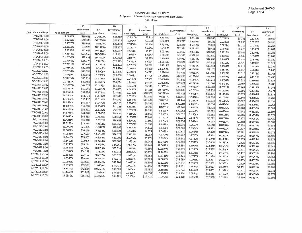
The first step in conducting the Probability of Dispatch method is to assign individual 1
generating plant investments to specific hours. In accordance with the procedures set 2
forth in the NARUC: Electric Utility Cost Allocation Manual,3 each plant’s total gross 3
investment and accumulated depreciation was assigned pro-ratably to each hour of the 4
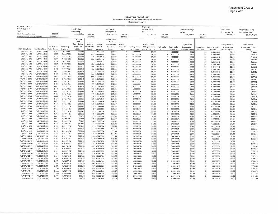
year based on each respective unit’s load (output) in that hour. My Attachment GAW-2 5
provides two pages of these hourly assignments. It should be noted that this exercise 6
actually assigns costs to 8,760 hours; however, my Attachment GAW-2 only 7
encompasses several of the first hours in the test year to avoid attachments exceeding 125 8
pages each. My filed workpapers contain the details of this assignment for each and 9
every hour of the test year. Page 1 of Attachment GAW-2 provides the assignment of 10
gross plant, while page 2 of this Attachment provides the assignment of each plant’s 11
depreciation reserve. This separate assignment is required due to differences in the net 12
book value of IPL’s various generation facilities. 13
14
Once hourly investment costs are known, these costs were then assigned to individual 15
rate classes on an hour-by-hour basis. As indicated earlier, IPL provided individual class 16
loads for each hour of the test year. As such, each class’ relative contribution to the total 17
system load in a given hour, is multiplied by the hourly generation investment cost. The 18
hourly class investment cost were then summed for all hours of the year to develop class 19
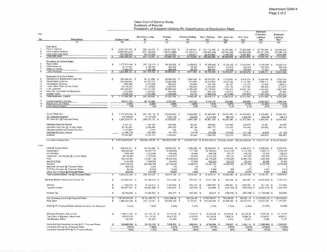
responsibility for IPL’s net generation plant. Attachment GAW-3 provides summaries of 20
the hourly assignment of generation costs to individual rate classes. The class assignment 21
to every hour of the test year are provided in my filed workpapers. 22
23
Q. PLEASE PROVIDE A SUMMARY OF THE RESULTS OBTAINED UTILIZING 24
THE PROBABILITY OF DISPATCH METHOD. 25
A. First it should be noted that the following summary and comparison utilizes all other 26
allocations and procedures used by Dr. Gaske in conducting his revised 12-CP CCOSS. 27
The following table provides an apples-to-apples comparison of Dr. Gaske’s revised 12-28
CP results to those obtained utilizing the Probability of Dispatch method: 29
3 1992 Edition, page 62.
17
1
2
3
4
5
6
7
8
9
10
11
12
13
14
15
16
17
As can be seen in the table above, there are significant differences for some classes and 18
minimal differences for other classes. For example, the residential rate of return 19
(“ROR”) increases from 2.48% to 4.00%, while several of the industrial classes RORs are 20
significantly reduced. A summary of my Probability of Dispatch CCOSS results are 21
provided in my Attachment GAW-4, while the details are provided in my filed 22
workpapers. 23
24
Q. CAN YOU QUALITATIVELY EXPLAIN WHY THE PROBABILITY OF 25
DISPATCH METHOD PRODUCES SIGNIFICANTLY DIFFERENT RESULTS 26
FOR SOME CLASSES? 27
A. Yes. IPL’s portfolio of generating assets is overwhelmingly comprised of base load coal 28
units that operate at very high capacity factors such that they provide energy to the 29
system throughout the year. At the same time, IPL has a much smaller investment in 30
intermediate and peaker units. The Probability of Dispatch method properly recognizes 31
CCOSS Comparison Utilizing IPL’s Procedures Except For The Allocation of Generation Plant
(Rate of Return At Current Rates) IPL
Revised Probability
Of Class 12-CP Dispatch
Residential RS 2.48% 4.00%Secondary Small SS 13.41% 13.71%Space Conditioning SH 2.79% 2.75%Space Conditioning-Schools SE 3.95% 6.63%Water Heating-Controlled CB -7.14% -7.10%Water Heating-Uncontrolled UW 2.87% 2.99%Secondary Large SL 7.26% 6.51%Primary PL 4.32% 2.48%Process Heating PH 3.13% 4.82%HLF-Primary HL1 3.93% 1.34%HLF-Sub-Tran HL2 3.50% 0.58%HLF-Tran HL3 3.24% -0.22%Automatic Protective Lighting APL -12.28% -13.45%Municipal Lighting MU1 29.89% 11.20% Total 4.88% 4.88%
18
the fact that IPL’s base load units are much more expensive and assigns these costs based 1
on its actual dispatch (operation) during the year. The 12-CP method does not recognize 2
the investment or operational characteristics of IPL’s generation portfolio as it simply 3
allocates the Company’s total combined investment in generation plant based on twelve 4
peak hours of the year. As such, the 12-CP method under-assigns generation costs to the 5
high load factor industrial classes and over-assigns costs to the lower load factor 6
residential class. 7
8
2. Base-Intermediate-Peak (“BIP”) Method 9
10
Q. PLEASE EXPLAIN HOW YOU CONDUCTED YOUR CCOSS UTILIZING THE 11
BASE-INTERMEDIATE-PEAK METHOD. 12
A. In order to reflect the capacity/energy trade-off inherent in IPL’s mix of generating 13
resources, each plant’s maximum capacity (mW) and output (mWh) during the test year 14
is required. Attachment GAW-5 provides the classification between energy and demand 15
for IPL’s generation plant under the BIP method. The BIP method evaluates each plant 16
based on its capacity factor and variable fuel costs to determine whether that plant 17
operates to serve primarily energy needs throughout the year, only peak loads, or is of an 18
intermediate type that serves both energy and peak load requirements. To illustrate, the 19
Petersburg units are clearly base load units in that they are “must run” units and operate 20
throughout the entire year. While the Harding Street units are also largely base load 21
units, I have classified this plant between energy and demand based on its capacity factor. 22
23
Q. DOES ATTACHMENT GAW-5 HELP EXPLAIN THE CAPACITY/ENERGY 24
TRADE-OFF CONSIDERATION USED BY ELECTRIC UTILITIES IN 25
DEVELOPING A PARTICULAR MIX OF GENERATING FACILITIES? 26
A. Yes. As can be seen in Attachment GAW-5, IPL’s larger, more expensive, generating 27
plants have high capacity factors and lower fuel costs. The large base load units run most 28
hours of the year supplying energy to all customers. In contrast, the smaller, high 29
operating (fuel) cost plants tend to have lower capacity factors meaning they are 30
primarily used to meet peak loads. Because the vast preponderance of IPL’s investment 31
19
in generation plant is associated with its base load units, a very large percentage (83.9%) 1
of generation plant is classified as energy-related under the BIP method. 2
3
Q. PLEASE PROVIDE A SUMMARY OF RESULTS OBTAINED UTILIZING THE 4
BASE-INTERMEDIATE-PEAK METHOD. 5
A. The following summary and comparison utilizes all other allocations and procedures used 6
by Dr. Gaske in conducting his 12-CP CCOSS. The following table provides an apples-7
to-apples comparison of Dr. Gaske’s 12-CP results to those obtained utilizing the BIP 8
method: 9
10
11
12
13
14
15
16
17
18
19
20
21
22
23
24
25
26
As can be seen in the table above, there are significant differences for some classes and 27
minimal differences for other classes. For example, the residential ROR increases from 28
2.48% to 3.73%, while several of the industrial classes RORs are significantly reduced. 29
A summary of my BIP CCOSS results are provided in my Attachment GAW-6, while the 30
details are provided in my filed workpapers. 31
CCOSS Comparison Utilizing IPL’s Procedures Except For The Allocation of Generation Plant
(Rate of Return At Current Rates) IPL
Revised
Class 12-CP BIP Residential RS 2.48% 3.73% Secondary Small SS 13.41% 13.26% Space Conditioning SH 2.79% 3.40% Space Conditioning-Schools SE 3.95% 5.53% Water Heating-Controlled CB -7.14% -8.18% Water Heating-Uncontrolled UW 2.87% 0.31% Secondary Large SL 7.26% 6.47% Primary PL 4.32% 3.46% Process Heating PH 3.13% 4.41% HLF-Primary HL1 3.93% 1.31% HLF-Sub-Tran HL2 3.50% 1.08% HLF-Tran HL3 3.24% 0.44% Automatic Protective Lighting APL -12.28% -13.23% Municipal Lighting MU1 29.89% 14.33% Total 4.88% 4.88%
20
3. Peak & Average (“P&A”) Method 1
2
Q. PLEASE EXPLAIN HOW YOU CONDUCTED YOUR CCOSS UTILIZING THE 3
P&A METHOD. 4
A. I used IPL’s test year retail load factor of 53.66% in order to weight the energy (average) 5
portion versus the peak portion of the P&A allocator. 6
7
Q. WHAT MEASURE OF PEAK DEMAND DID YOU USE FOR THE DEMAND 8
PORTION OF THE P&A ALLOCATOR? 9
A. I used Dr. Gaske’s class contributions to the 1-CP demand rather than the 12-CP demand 10
to reflect the peak nature and responsibility of class loads.4 I have selected this measure 11
of peak demand because the 12-CP incorporates peak and non-peak months; i.e., spring 12
and fall demands. In my opinion, the use of class contributions to 1-CP better reflect the 13
spirit and concepts of the P&A method. 14
15
Q. WHAT ARE THE RESULTS OF YOUR CCOSS UTILIZING THE P&A 16
METHOD TO ALLOCATE GENERATION COSTS? 17
A. The following summary and comparison utilizes all other allocations and procedures used 18
by Dr. Gaske in conducting his 12-CP CCOSS. The following table provides an apples-19
to-apples comparison of Dr. Gaske’s 12-CP results to those obtained utilizing the P&A 20
method: 21
22
23
24
25
26
27
28
29
30
4 Per response to OUCC-18-1, Attachment 2.
21
1
2
3
4
5
6
7
8
9
10
11
12
13
14
15
16
17
Unlike the Probability of Dispatch and BIP methods, the P&A approach produces results 18
relatively similar to those obtained under the 12-CP method. A summary of my P&A 19
CCOSS results are provided in my Attachment GAW-7, while the details are provided in 20
my filed workpapers. 21
22
Q. EARLIER IN YOUR TESTIMONY YOU INDICATED THAT THE 23
PROBABILITY OF DISPATCH, BIP, AND P&A METHODS MAY NOT 24
PROPERLY RECOGNIZE CLASS VARIANCES IN VARIABLE GENERATION 25
COSTS. HAVE YOU EXAMINED WHETHER THERE ARE MATERIAL 26
DIFFERENCES IN CLASS FUEL COSTS WHEN ANALYZED ON AN HOURLY 27
BASIS? 28
A. Yes I have. As discussed earlier, IPL provided each generation plant’s hourly output 29
during the test year. In addition, in response to OUCC-18-9, Attachment 1, the Company 30
provided monthly fuel costs (per mWh) for each plant. With this data, I was able to 31
CCOSS Comparison Utilizing IPL’s Procedures Except For The Allocation of Generation Plant
(Rate of Return At Current Rates) IPL
Revised
Class 12-CP P&A Residential RS 2.48% 2.64% Secondary Small SS 13.41% 13.39% Space Conditioning SH 2.79% 3.71% Space Conditioning-Schools SE 3.95% 5.55% Water Heating-Controlled CB -7.14% -7.25% Water Heating-Uncontrolled UW 2.87% 2.92% Secondary Large SL 7.26% 7.37% Primary PL 4.32% 4.35% Process Heating PH 3.13% 4.77% HLF-Primary HL1 3.93% 2.88% HLF-Sub-Tran HL2 3.50% 2.28% HLF-Tran HL3 3.24% 2.33% Automatic Protective Lighting APL -12.28% -12.80% Municipal Lighting MU1 29.89% 21.02% Total 4.88% 4.88%
22
calculate hourly fuel costs by individual generating plant. These hourly fuel costs were 1
then assigned to individual rate classes on an hour-by-hour basis based on class hourly 2
loads also discussed previously.5 The end result of this analysis yielded very similar 3
hourly fuel costs across all classes such that all classes’ fuel costs are within 2.00% of the 4
system average annual fuel cost as shown below6: 5
6
7
8
9
10
11
12
13
14
15
16
17
Q. WHAT ARE YOUR CONCLUSIONS REGARDING THE PROPER 18
ALLOCATION OF IPL’S GENERATION PLANT? 19
A. IPL’s portfolio of generating assets is comprised predominately of large base load units 20
that serve the energy needs of IPL throughout the entire year. While IPL does indeed 21
rely upon intermediate and peaker units to some degree, the dollar investment in these 22
facilities pale in comparison to its base load investments. The Probability of Dispatch 23
and BIP methods are very detailed approaches that are theoretically sound and reasonably 24
reflect the capacity/energy trade-off in generation facilities specific to IPL’s investment. 25
As such, these two methods are the most “accurate” methods from a cost causation 26
perspective. While the P&A method is much simpler in its data requirements as well as 27
in its analytical application, and is admittedly somewhat arbitrary, it too recognizes the 28
5 The class hourly loads were provided at the sales (meter) level. Each class’ loads were adjusted for losses back to generation based on each class’ respective energy loss factor as provided in response to OUCC-18-1, Attachment 2. 6 The details of this analysis is provided in my filed workpapers.
IPL Class Hourly Fuel Costs Fuel Cost Deviation From
Class Per mWh Sys. Average Residential RS $26.30 -0.9%Secondary Small SS $26.73 0.7%Space Conditioning SH $26.61 0.2%Space Conditioning-Schools SE $26.42 -0.5%Secondary Large SL $26.97 1.6%Primary PL $26.28 -1.0%Process Heating PH $26.04 -1.9%HLF-Primary HL1 $26.35 -0.8%HLF-Sub-Tran HL2 $26.50 0.2%HLF-Tran HL3 $26.45 -0.4%Total $26.55 --
23
fact that much of IPL’s generation resources are utilized to meet energy requirements 1
throughout the year. It is my opinion that each of these methods should be considered in 2
evaluating class profitability. Furthermore, because the 12-CP method does not produce 3
results materially different than the P&A method, this approach can also be considered in 4
the context of class profitability. 5
6
Q. FOR THE RECORD, PLEASE PROVIDE A SUMMARY OF CLASS RATES OF 7
RETURN UNDER EACH OF THE FOUR GENERATION ALLOCATION 8
METHODOLOGIES YOU HAVE DISCUSSED. 9
A. The following table provides class rates of return at current rates utilizing all other 10
aspects of Dr. Gaske’s CCOSS (except for the minor correction to lighting revenues): 11
12
13
14
15
16
17
18
19
20
21
22
23
24
25
26
27
28
29
30
31
CCOSS Comparison Utilizing IPL’s Procedures Except For The Allocation of Generation Plant
(Rate of Return At Current Rates)
Probability of
12-CP P&A BIP Dispatch
Residential RS 2.48% 2.64% 3.73% 4.00%
Secondary Small SS 13.41% 13.39% 13.26% 13.71%
Space Conditioning SH 2.79% 3.71% 3.40% 2.75%
Space Conditioning - Schools SE 3.95% 5.55% 5.53% 6.63%
Water Heating - Controlled CB -7.14% -7.25% -8.18% -7.10%
Water Heating - Uncontrolled UW 2.87% 2.92% 0.31% 2.99%
Municipal Lighting MU1 29.89% 21.02% 14.33% 11.20%
Total Jurisdictional 4.88% 4.88% 4.88% 4.88%
24
B. Transmission Plant 1
2
Q. PLEASE EXPLAIN THE THEORIES ON HOW TRANSMISSION-RELATED 3
PLANT SHOULD BE ALLOCATED WITHIN AN EMBEDDED CCOSS. 4
A. There are two general philosophies relating to the proper allocation of transmission-5
related plant. The first philosophy is based on the premise that transmission facilities are 6
nothing more than an extension of generation plant in that transmission facilities simply 7
act as a conduit to provide power and energy from distant generating facilities to a 8
utility’s load center (specific service area). That is, generation facilities are often located 9
well away from load centers and near the resources required to operate generation 10
facilities. For example, coal generation facilities are commonly located near water 11
sources for steam and cooling or near coal mines and/or rail facilities. Similarly, natural 12
gas generators must be located in close proximity to large natural gas pipelines. 13
14
The second philosophy relates to the physical capacity of transmission lines. That is, 15
transmission facilities have a known and measurable load capability such that customer 16
contributions to peak load should serve as the basis for allocating these transmission 17
costs. While there is no doubt that any given electricity conductor (i.e., a transmission 18
line) has a physical load carrying capability, this rationale fails to recognize cost 19
causation in three regards. 20
21
First, an allocation based simply on contributions to a few hours of peak load fails to 22
recognize the fact that transmission facilities are indeed an extension of generation 23
facilities and are used to move the energy produced by the generators from remote 24
locations to where customers actually consume electricity. Second, and similar to the 25
concept of base load units producing energy to serve customers throughout the year, a 26
peak responsibility approach based on one or only a few hours of maximum demand fails 27
to recognize that transmission facilities are used virtually every hour of an entire year and 28
not just during periods of peak load. Third, any assumption that transmission costs are 29
related to peak load implies that there is a direct and linear relationship between cost and 30
load. In other words, one must assume that if load increases, the cost of transmission 31
25
facilities increases, in a direct and linear manner. This is simply not the case since there 1
are significant economies of scale associated with high voltage transmission lines. 2
3
Q. WHAT METHOD DID DR. GASKE USE TO ALLOCATE IPL’S 4
TRANSMISSION-RELATED COSTS? 5
A. Dr. Gaske allocated transmission-related costs based on the 12-CP method. 6
7
Q. WHAT IS YOUR OPINION REGARDING DR. GASKE’S USE OF THE 12-CP 8
METHOD TO ALLOCATE TRANSMISSION-RELATED COSTS? 9
A. In my opinion, the 12-CP approach strikes a reasonable balance between the two general 10
philosophies that were discussed above as it relates to the cost causation and allocation of 11
transmission-related costs. 12
13
C. Distribution Plant 14
15
Q. PLEASE EXPLAIN THE PHRASE "CLASSIFICATION OF DISTRIBUTION 16
PLANT." 17
A. It is generally recognized that there are no energy-related costs associated with 18
distribution plant. That is, the distribution system is designed to meet localized peak 19
demands. However, largely as a result of differences in customer densities throughout a 20
utility's service area, electric utility distribution plant sometimes is classified as partially 21
demand-related and partially customer-related. 22
23
Q. WHY IS DISTRIBUTION PLANT SOMETIMES CLASSIFIED AS PARTIALLY 24
CUSTOMER-RELATED AND PARTIALLY DEMAND-RELATED? 25
A. Even though investment is made in distribution plant and equipment to meet the needs of 26
customers at their required power levels, there may be considerable differences in both 27
customer densities and the mix of customers throughout a utility’s service area. 28
Therefore, if one were to allocate distribution plant investment based simply on class 29
contributions to peak demand, an inequitable allocation of these costs may result. As a 30
hypothetical, suppose a utility serves both an urban area and a rural area. In this 31
26
situation, many customers’ electrical needs are served with relatively few miles of 1
conductors, few poles, etc. in the urban area, while many more miles of conductors, more 2
poles, etc. are required to serve the requirements of relatively few customers in the rural 3
area. If the distribution of classes of customers (class customer mix) is relatively similar 4
in both the rural and urban areas, there is no need to consider customer counts (number 5
of customers) within the allocation process, because all classes use the utility’s joint 6
distribution facilities proportionately across the service area. However, if the customer 7
mix is such that commercial and industrial customers are predominately clustered in the 8
more densely populated urban area, while the less dense (rural) portion of the service 9
territory consists almost entirely of residential customers, it may be unreasonable to 10
allocate the total Company’s distribution investments based solely on demand; i.e., a 11
large investment in many miles of line is required to serve predominately residential 12
customers in the rural area while the commercial and industrial electrical needs are met 13
with much fewer miles of lines in the urban area. Under this circumstance, an allocation 14
of costs based on a weighting of customers and demand can be considered equitable and 15
appropriate. 16
17
Q. PLEASE PROVIDE AN EXAMPLE THAT ILLUSTRATES THE CONCEPTS OF 18
DENSITY AND CLASS CUSTOMER MIX AS THEY RELATE TO COST 19
ALLOCATIONS. 20
A. As a starting point, it is important to understand absolute and relative class relationships 21
of an electric utility’s number of customers, energy requirements, and maximum loads 22
(demands). In terms of simple customer counts, the number of residential accounts 23
make-up the overwhelming majority of any retail electric utility’s number of customers. 24
However, because residential customers tend to be small volume users compared to 25
commercial and industrial customers, the residential class is responsible for a 26
significantly smaller percentage of total kWH energy supplied or peak loads on the 27
system. For example, in IPL’s system, the following characteristics are exhibited: 28
29
30
31
27
1
2
3
4
5
6
7
While the table above shows the relative class differences between number of customers, 8
energy usage, and peak demands, the following table illustrates the absolute size 9
differences between IPL’s different types of customers: 10
11
12
13
14
15
16
17
With the above relationships explained, in order to understand the concepts of density 18
and class customer mix, consider examples of two hypothetical electric utilities each of 19
which are comprised of only two distribution lines: one line serving a densely populated 20
area (urban) and another line serving a sparsely populated area (rural). Furthermore, for 21
simplicity and explanatory purposes, assume there are only two classes of customers for 22
each utility: residential and commercial/industrial with the following characteristics: 23
24
25
26
27
28
29
30
31
Percentage of Total Jurisdictional Distribution System
Category
Customers
kWh
Peak Demand
(NCP) Residential 88.1% 38.3% 55.3% Comm./Ind. Distribution Voltage 11.7% 61.2% 44.2% Lighting 0.2% 0.5% 0.5%
Category
Average Annual kWh
Per Customer
(kWh) Residential 11,869 Comm./Ind. Distribution Voltage 143,120
Absolute Relative Number of Peak Peak Load Number of Peak
Class Customers Load Per Customer Customers Load Residential 110 550 5 83% 33% Comm./Ind. 22 1,100 50 17% 67% Total 132 1,650 -- 100% 100%
28
Utility A: 1
For Utility A, assume all commercial/industrial customers are located on the 2
urban (densely populated) distribution line such that the rural line only serves residential 3
customers as shown graphically below: 4
5
6
7
29
Because the urban line is much shorter in total distance, yet, serves the majority of 1
customers (and loads) and many more miles of line are required to serve relatively few 2
residential only customers in rural areas, it would be unfair, and inconsistent with cost 3
causation to allocate total system line costs only on utilization (kW) because 4
commercial/industrial customers arguably do not cause costs to be incurred for the rural 5
portion of the system. As such, some weighting of relative number of customers and 6
utilization is appropriate to allocate total system line costs. 7
8
Utility B: 9
For Utility B, assume that the relative mix of customers is evenly distributed 10
between the urban and rural lines. In other words, this utility’s configuration of 11
customers is as follows: 12
13
14
15
16
17
18
19
20
Number of Customers Urban Line Rural Line
Class Amount Percent Amount Percent Residential 100 83% 10 83% Comm./Ind. 20 17% 2 17% Total 120 100% 12 100%
30
1
2
As can be seen in the above table and charts, the relative imposition of costs across the 3
two classes for Utility B is the same for the urban and rural lines. That is, while there are 4
more absolute residential customers than commercial/industrial customers on both the 5
urban and rural lines, the proportion (mix) of customers is the same between urban and 6
rural. As such, an allocation of total system lines costs based on utilization (maximum 7
loads) is appropriate such that no consideration of customer counts is needed or desired. 8
Indeed, if distribution costs are classified and allocated partially on number of customers, 9
the residential class will be over burdened with cost responsibility creating a subsidy for 10
commercial/industrial customers. 11
12
Q. DOES THE CLASSIFICATION OF DISTRIBUTION PLANT INVESTMENT AS 13
PARTIALLY CUSTOMER-RELATED AND PARTIALLY DEMAND-RELATED 14
REFLECT ANY RELATIVE COST (PER MILE) DIFFERENCES BETWEEN 15
URBAN AND RURAL AREAS? 16
A. No. It is generally more expensive to install a mile of distribution circuit in an urban area 17
than in a rural area. However, although this cost difference may be substantial, this cost 18
difference is usually ignored due to record keeping limitations, in that all costs are simply 19
assumed to be uniform (averaged) across the rural and urban portions of a service area. 20
31
Q. DO YOUR EXAMPLES DISCUSSED ABOVE IMPLY THAT IT COSTS MORE 1
TO SERVE RURAL CUSTOMERS THAN URBAN CUSTOMERS AND THAT 2
PERHAPS A UTILITY’S RURAL CUSTOMERS SHOULD PAY MORE PER 3
UNIT THAN URBAN CUSTOMERS? 4
A. While it is possible that it technically costs more to serve a rural customer versus an 5
urban customer, regulatory policy in the United States has generally been not to price 6
discriminate based on customer densities, urban versus rural, or other geographic 7
differences. Rather, regulatory policy has been such that classes of customers with 8
similar usage and/or load characteristics are established for pricing purposes. In fact, 9
during my 34-plus years practicing utility costing and pricing across the Country, I have 10
not seen a rate structure that discriminates based on customer densities or other 11
geographic characteristics. 12
13
Q. IS THERE ACADEMIC SUPPORT FOR YOUR EXPLANATION AND 14
CONCEPTS REGARDING CUSTOMER DENSITIES AND CLASS CUSTOMER 15
MIXES? 16
A. Yes. In the well-known and often referenced, treatise Principles of Public Utility Rates, 17
Professor James Bonbright states that there: 18
is the very weak correlation between the area (or the mileage) of a 19 distribution system and the number of customers served by this system. 20 For it makes no allowance for the density factor (customers per linear mile 21 or per square mile). Our casual empiricism is supported by a more 22 systematic regression analysis in (Lessels, 1980) where no statistical 23 association was found between distribution costs and number of 24 customers. Thus, if the company’s entire service area stays fixed, an 25 increase in number of customers does not necessarily betoken any increase 26 whatever in the costs of a minimum-sized distribution system.7 27 28
Q. BEFORE I CONTINUE, IS IPL’s DISTRIBUTION SYSTEM COMPRISED OF 29
VARIOUS SUB-SYSTEMS? 30
A. Yes. As is the case with virtually every electric utility, IPL’s overall distribution system 31
is comprised of a primary voltage system and a secondary voltage system. The primary 32
7 Bonbright, Principles of Public Utility Rates, Second Edition, page 491.
32
system operates at higher voltage levels than the secondary system and generally consists 1
of plant and equipment between the substations and transformers. The lower voltage 2
secondary system can be thought of as operating downstream from the primary system 3
and delivers electricity to small end-users. 4
5
Q. BRIEFLY DESCRIBE THE TYPES OF INVESTMENT (EQUIPMENT) 6
UTILIZED IN IPL’s DISTRIBUTION SYSTEM. 7
A. For accounting purposes, IPL’s distribution plant is grouped into various accounts. 8
These accounts include: Land and Land Rights (Account 360); Structures and 9
Improvements (Account 361); Station Equipment (Account 362); Poles, Towers and 10
Q. HAVE YOU CONDUCTED ANALYSES TO DETERMINE IF A 1
CLASSIFICATION OF DISTRIBUTION PLANT AS PARTIALLY CUSTOMER-2
RELATED IS APPROPRIATE FOR IPL? 3
A. Yes, I have. 4
5
Q. PLEASE EXPLAIN. 6
A. Dr. Gaske has made an a priori assumption that it is appropriate to allocate a portion of 7
its distribution plant based on customer counts and a portion based on demand levels. As 8
indicated earlier, the only reason why it may be appropriate to allocate a portion of 9
distribution plant expenses based on number of customers, rather than peak demand, is 10
due to the possibility that the mix of customers varies significantly across the customer 11
density levels within IPL’s service territory. In this regard, I evaluated this assumption 12
by conducting an analysis of the distribution, or mix, of IPL’s customer classes across its 13
service area. 14
15
Through discovery, the Company provided a data base of the number of customers by 16
rate schedule for each postal zip-code within its service area. I then evaluated the mix of 17
customers by rate class for each postal zip-code within the IPL service area. In order to 18
evaluate whether any differences exist in the distribution of customers across various 19
customer density areas, I calculated the number of total IPL distribution customers 20
(excluding lighting customers) per square mile for each non-Post Office Box zip-code to 21
serve as a measure of density for relatively small geographic areas. I was then able to 22
readily compare IPL’s mix of customers throughout its service area and delineate 23
between sparsely populated and densely populated areas (in terms of number of IPL 24
customers). As a further refinement, I also evaluated the distribution of customers on a 25
stratified basis. That is, for each customer group (residential, small 26
commercial/industrial, and large commercial/industrial)8 I separated small geographical 27
areas (zip codes) into four separate strata (highest to lowest customer densities). I 28
8 Dr. Gaske developed his non-coincident peak (“NCPs”) demands based on these same three customer groups, which then serves as the basis for his allocation of the “demand” portion of each distribution plant account.
34
examined each stratum (by customer group) to determine if any significant differences in 1
customer mix occur within each stratum. 2
3
This analysis of the distribution of the various customer groups by density provided a 4
basis to determine whether: (a) utilization alone (demand) is an appropriate and fair 5
method to allocate distribution costs; or, (b) whether a weighting of customers and 6
utilization (demand) is appropriate in order to reasonably reflect the imposition or 7
causation of costs. 8
9
If there is any basis for a customer classification of distribution plant, this analysis should 10
show a negative correlation between the residential customer mix (residential percentage 11
of total customers) and density across IPL’s service area. In other words, the percentage 12
of residential customers (by zip-code) should decline as customer density per square mile 13
increases from the least dense areas to the most dense areas of IPL’s service territory. 14
Similarly, if Dr. Gaske’s assumption is correct, you should see a distinct positive 15
correlation between non-residential customer mixes and customer densities by zip-code. 16
The graph below shows the percentage of total customers by rate group (Y axis) 17
compared to total customers per square mile (X axis): 18
19
20
21
22
23
24
25
26
27
28
29
30
35
36
As can be seen in the graph above, there is absolutely no correlation or trend between the 1
distribution of customers (customer mix) and density levels for any of the three customer 2
groups. Indeed, and as shown in the graph, the correlation coefficients for all three 3
customer groups are essentially zero. 4
5
As discussed earlier, I also analyzed this data on a stratified basis. A summary of the 6
approach and data utilized for the stratification analysis is provided below: 7
8
9
10
11
12
13
14
15
16
17
18
19
20
21
22
Q. WHAT ARE YOUR FINDINGS AS A RESULT OF THIS ANALYSIS? 23
A. IPL’s customers are dispersed in a reasonably proportional manner throughout its service 24
area. In fact, the distribution of residential customers is somewhat greater in the more 25
densely populated zip codes than the less densely populated zip codes, which is contrary 26
to the hypothesis and is opposite of what would be expected if one were to accept the 27
notion that distribution investment should be classified as partially customer-related. 28
As important is the fact that in the less dense areas of IPL’s service territory (which 29
requires more miles of distribution lines and number of poles to serve fewer customers), 30
9 Excludes Lighting.
Percent of Total Distribution Customers9
Class
Customers Per Sq.
Mile (Density)
Count Of Zip
Codes
Simple Avg.
Weighted Avg.
Number
% of Class
Residential Strata 1 1,704 Min to 4,944 Max 13 86.50% 87.38% 191,066 40.8% Strata 2 1,025 Min to 1,703 Max 13 85.24% 86.00% 175,414 37.5% Strata 3 138 Min to 1,024 Max 13 87.25% 87.69% 87,270 18.7% Strata 4 Less Than 138 14 83.25% 84.87% 14,090 3.00% Total 53 467,840 100.0% Small Comm./Ind. Strata 1 1,704 Min to 4,944 Max 13 12.36% 11.72% 25,632 39.2% Strata 2 1,025 Min to 1,703 Max 13 13.46% 12.83% 26,177 40.0% Strata 3 138 Min to 1,024 Max 13 11.69% 11.27% 11,218 17.2% Strata 4 Less Than 138 14 15.61% 14.10% 2,340 3.6% Total 53 65,367 100.0% Large Comm./Ind. Strata 1 1,704 Min to 4,944 Max 13 1.14% 0.90% 1,959 35.3% Strata 2 1,025 Min to 1,703 Max 13 1.31% 1.17% 2,382 42.9% Strata 3 138 Min to 1,024 Max 13 1.06% 1.04% 1,034 18.6% Strata 4 Less Than 138 14 1.14% 1.03% 171 3.2% Total 53 5,546 100.0%
37
the Company actually serves a larger percentage of commercial/industrial customers than 1
in the more densely populated areas within IPL’s service territory. 2
3
As a result of these analyses, it cannot be said that the less populated portions of IPL’s 4
service area (which require significant investment to serve few customers) are 5
disproportionately required to serve any one class of customers. As such, IPL’s 6
distribution plant and expenses should be assigned to classes based only on utilization 7
(peak demand) and any consideration of customer counts is improper for the allocation of 8
distribution plant. Therefore, my studies indicate that IPL’s distribution plant should be 9
classified as 100% demand-related. 10
11
Q. DOES THE NARUC ELECTRIC COST ALLOCATION MANUAL INDICATE IF 12
AN A PRIORI ASSUMPTION IS APPROPRIATE REGARDING WHETHER 13
DISTRIBUTION COSTS MUST BE CLASSIFIED AS PARTIALLY CUSTOMER-14
RELATED AND PARTIALLY DEMAND-RELATED? 15
A. No. In fact, the NARUC Manual (published in 1992) states the following: 16
To ensure that costs are properly allocated, the analyst must first classify 17 each account as demand-related, customer-related, or a combination of 18 both. The classification depends upon the analyst’s evaluation of how the 19 costs in these accounts were incurred. In making this determination, 20 supporting data may be more important than theoretical considerations. 21 22 Allocating costs to the appropriate groups in a cost study requires a special 23 analysis of the nature of distribution plant and expenses. (page 89) 24
25
Q. HAS NARUC PROVIDED MORE RECENT GUIDANCE CONCERNING THE 26
CLASSIFICATION OF DISTRIBUTION PLANT THAN WHAT WAS 27
PUBLISHED IN THE 1992 NARUC ELECTRIC COST ALLOCATION 28
MANUAL? 29
A. Yes. The 1992 NARUC Manual was written in an era when all retail utility services 30
were bundled (generation, transmission and distribution). Subsequent to the unbundling 31
of retail rates in the mid to late 1990’s by several state jurisdictions, NARUC 32
commissioned a study to examine the costing and pricing of electric distribution service 33
in further detail. In December 2000, NARUC published a report entitled: Charging For 34
38
Distribution Services: Issues in Rate Design. As part of the Executive Summary this 1
report states: 2
The usefulness of cost analyses of the distribution system in designing rate 3 structures and setting rate levels depends in large measure upon the 4 manner in which the studies are undertaken. Cost studies (both marginal 5 and embedded) are intended, among other things, to determine the nature 6 and causes of costs, so that they can then be reformulated into rates that 7 cost-causers can pay. Such studies must of necessity rely on a host of 8 simplifying assumptions in order to produce workable results; this is 9 especially true of embedded cost studies. Moreover, it is often the case 10 that many of the costs (e.g., administrative and general) that distribution 11 rates recover are not caused by provision of distribution service, but are 12 assigned to it arbitrarily. Too great dependence on cost studies is to be 13 captured by their underlying assumptions and methodological flaws. 14 Utilities and commissions should be cautious before adopting a particular 15 method on the basis of what may be a superficial appeal. More important, 16 however, is the concern that a costing method, once adopted, becomes the 17 predominant and unchallenged determinant of rate design. (page 67) 18 19
With specific regard to classification and allocation of certain distribution plant (poles, 20
wires and transformers), Chapter IV of this report is devoted to the costing of distribution 21
services. With respect to embedded cost analyses this updated NARUC report states: 22
There are a number of methods for differentiating between the customer 23 and demand components of embedded distribution plant. The most 24 common method used is the basic customer method, which classifies all 25 poles, wires, and transformers as demand-related and meters, meter-26 reading, and billing as customer-related. This general approach is used in 27 more than thirty states. A variation is to treat poles, wires, and 28 transformers as energy-related driven by kilowatt-hour sales but, though it 29 has obvious appeal, only a small number of jurisdictions have gone this 30 route. 31 32 Two other approaches sometimes used are the minimum size and zero-33 intercept methods. The minimum size method operates, as its name 34 implies, on the assumption that there is a minimum-size distribution 35 system capable of serving customers minimum requirements. The costs of 36 this hypothetical system are, so the argument goes, driven not by customer 37 demand but rather by numbers of customers, and therefore they are 38 considered customer costs. The demand-related cost portion then is the 39 difference between total distribution investment and the customer-related 40 costs. The zero-intercept approach is a variation on the minimum size. 41 Here the idea is to identify that portion of plant that is necessary to give 42 customers access but which is incapable of serving any level of demand. 43 The logic is that the costs of this system, because it can serve no demand 44
39
and thus is not demand-related, are necessarily customer-related. 1 However, the distinction between customer and demand costs is not 2 always clear, insofar as the number of customers on a system (or particular 3 area of a system) will have impacts on the total demand on the system, to 4 the extent that their demand is coincident with the relevant peak (system, 5 areal, substation, etc.). 6 7 Any approach to classifying costs has virtues and vices. The first potential 8 pitfall lies in the assumptions, explicit and implicit, that a method is built 9 upon. In the basic customer method, it is the a priori classification of 10 expenditures (which may or may not be reasonable). In the case of the 11 minimum-size and zero-intercept methods, the threshold assumption is 12 that there is some portion of the system whose costs are unrelated to 13 demand (or to energy for that matter). From one perspective, this notion 14 has a certain intuitive appeal these are the lowest costs that must be 15 incurred before any or some minimal amount of power can be delivered 16 but from another viewpoint it seems absurd, since in the absence of any 17 demand no such system would be built at all. Moreover, firms in 18 competitive markets do not indeed, cannot price their products according 19 to such methods: they recover their costs through the sale of goods and 20 services, not merely by charging for the ability to consume, or access. 21 (pages 29 & 30) 22
23 24
In summary, when all of the facts and guidelines are known, it is clear to me that: (a) 25
data and analysis specific to each utility is more appropriate and preferred over an a 26
priori assumption that distribution plant must be partially customer-related; and, (b) 27
many (if not most) state regulatory commissions endorse a method in which all 28
distribution plant from substations through line transformers is classified and allocated 29
based solely on demand. A copy of the entire Chapter (IV) from the 2000 NARUC 30
Publication discussing costing studies is provided in my Attachment GAW-8. 31
32
Q. WHY IS THE CLASSIFICATION OF DISTRIBUTION PLANT IMPORTANT IN 33
CCOSS ANALYSES? 34
A. The classification of distribution plant may be the single most important factor affecting 35
class rates of return. To illustrate the importance of this issue, consider the residential 36
class: whereas this class may account for only 40% to 50% of peak demand, it is 37
responsible for a much higher percentage of the number of customers. Therefore, given 38
40
the level of investment associated with distribution plant, wide variations in class rates of 1
return can result from different customer/demand classifications. 2
3
Q. HOW DID DR. GASKE CLASSIFY DISTRIBUTION PLANT BETWEEN 4
CUSTOMER-RELATED AND DEMAND-RELATED COMPONENTS? 5
A. In response to OUCC-18-17 and OUCC-18-18, the Company indicated that its fixed asset 6
accounts records do not contain data relating to the installed footage of overhead and 7
underground conductors. As such, in response to OUCC-18-20, Dr. Gaske indicated that 8
he used replacement costs provided by IPL engineering personnel. 9
10
In other words, the Company does not maintain records in sufficient detail in order to 11
conduct studies based on actual costs and circuit miles of its distribution system. This 12
data is critical in classifying distribution plant under industry accepted practices. Rather, 13
Dr. Gaske was forced to rely upon estimates of current costs provided by IPL’s 14
engineering staff. I will discuss these deficiencies later in my testimony. 15
16
When a decision is made to classify a portion of distribution plant as customer-related 17
and a portion as demand-related, there are two industry accepted methods: the first is 18
known as the Minimum-Size approach while the second is known as the Zero-Intercept 19
approach. Dr. Gaske has attempted to utilize the Minimum-Size approach. Under this 20
method, the cost per unit (per pole or per circuit mile) of the minimum-sized equipment 21
actually installed is multiplied by the total number of units within the distribution system 22
(poles or circuit miles) which then serves as the total minimum system cost for a 23
particular distribution plant account. This total minimum system cost is then divided by 24
the total cost for the account such that the quotient serves as the customer percentage; i.e., 25
the minimum-size cost divided by the total cost equals the customer percentage. 26
27
There is a significant bias embedded within the so-called Minimum-Size method in that 28
the theory underlying both the Minimum-Size and Zero-Intercept methods is that there is 29
some level of cost required to simply connect customers with no load. In other words, 30
the loads that customers place on the system are related to peak demand such that there 31
41
are some costs required to simply connect customers to the system. The bias that results 1
under the Minimum-Size approach is that even the smallest sized conductor actually 2
installed has load carrying capability, and in fact, is installed to meet the collective loads 3
of the customers on a particular distribution line segment. Therefore, there is a 4
substantial level of demand-related costs within the “minimum-size” costs used within 5
this method. 6
7
Q. DO YOU HAVE DISAGREEMENTS REGARDING DR. GASKE’S MINIMUM-8
SIZE STUDIES RELATING TO SPECIFIC ACCOUNTS? 9
A. Yes. As is typically the case, Dr. Gaske has conducted separate analyses for Account 364 10
With regard to Dr. Gaske’s Minimum-Size analyses for distribution poles, he has used a 12
30-foot pole as a “minimum-size” secondary voltage pole and a 35-foot pole as a 13
“minimum-size” primary voltage poles. While the Company may indeed typically use 30 14
to 35-foot poles as a minimum, it must recognized that the reason for these minimum 15
heights is to accommodate telecommunication lines and cables on the same pole, which 16
are typically installed below the energized electrical lines. In response to OUCC-18-21, 17
the Company’s design standards require a minimum separation of 40 inches between 18
telecommunication cables and energized lines for secondary voltage poles and 40-60 19
inches for primary voltage poles. Because of this required separation to accommodate 20
telecommunication carriers, IPL’s distribution poles are clearly longer than they 21
otherwise would be. This has nothing to do with the need to simply connect electrical 22
customers, but rather, is no more than an accommodation for telecommunication 23
infrastructure. 24
25
In addition, the Company was able to provide an inventory of its actual distribution poles 26
by height in response to OUCC-18-20. This asset inventory report indicates that IPL has 27
15, 18, 20, and 25-foot poles actually installed in its distribution system which are clearly 28
less expensive than a 30-foot pole.10 29
10 It should be remembered that the cost used by Dr. Gaske are engineering estimates of replacement costs such that IPL’s engineers only provided cost estimates for poles as short as 30 feet.
42
Q. PLEASE DISCUSS YOUR DISAGREEMENTS WITH DR. GASKE’S MINIMUM-1
SIZE ANALYSES SPECIFIC TO OVERHEAD AND UNDERGROUND 2
CONDUCTORS. 3
A. In order to explain my disagreements with Dr. Gaske’s Minimum-Size analyses as it 4
relates to overhead and underground conductors, one must understand how an electrical 5
circuit is configured. All electric distribution systems are comprised of both single-phase 6
and multi-phase (3-phase) circuits. While some single-phase circuits are comprised of 7
only two wires, current practices are to generally install three-wire single-phase circuits, 8
while virtually all three-phase circuits require four conductors. Furthermore, three-phase 9
circuits tend to be comprised of larger size conductors than do single-phase circuits. In 10
this regard, the NARUC: Electric Cost Allocation Manual states the following as it 11
relates to studies conducted using the Minimum-Size approach: 12
Overhead Conductors – 13 Multiply average installed book cost per mile of minimum size 14 conductor by the number of circuit miles to determine the customer 15 component. Balance of plant account is demand component. 16 (Note: two conductors in minimum system.)11 17
18
Underground Conductors – 19
Multiply average installed book cost per mile of minimum size 20 cable by the circuit miles to determine the customer component. 21 Balance of plant Account 367 is demand component. (Note: one 22 cable with ground sheath is minimum system.) Account 366 23 conduit is assigned, based on ratio of cable account.12 24
25
In examining the data utilized by Dr. Gaske it is apparent that he has not considered or 26
reflected circuit miles, nor has he utilized a two-wire circuit as set forth in the NARUC 27
Manual for a minimum-size circuit. In response to OUCC-18-20, the data provided to 28
Dr. Gaske by IPL includes the total footage associated with various types of both single-29
bare wire as well as multiplex cables. In other words, single-bare wire is a single wire 30
that is only a component of a complete circuit. Multiplex cables are comprised of 31
numerous conductors (usually three to four) within the cable that do normally constitute 32 11 Electric Utility Cost Allocation Manual, National Association of Regulatory Utility Commissioners, 1992 Edition, page 91. 12 Id.
43
an entire circuit. Dr. Gaske has mismatched single wires and complete circuits within his 1
analysis. Furthermore, and as indicated earlier, because of the limited information 2
available to Dr. Gaske it is impossible to determine the number of total circuit miles as 3
well as what the cost of a two-wire circuit mile would be. 4
5
Q. ARE YOU AWARE OF ANY OTHER CASE IN INDIANA IN WHICH 6
SUFFICIENT RECORDS WERE NOT AVAILABLE TO PROPERLY CONDUCT 7
A MINIMUM-SIZE OR ZERO-INTERCEPT ANALYSIS TO SEPARATE 8
DISTRIBUTION COSTS BETWEEN CUSTOMER-RELATED AND DEMAND-9
RELATED COMPONENTS? 10
A. Yes. In Cause No. 43526 involving Northern Indiana Public Service Company 11
(“NIPSCO”), the Commission’s Final Order states: 12
Mr. Greneman [Company witness] testified that primary lines, secondary 13 lines and line transformers were classified as 100% demand-related 14 because NIPSCO’s property records were not sufficiently detailed as to 15 reliably support a zero-intercept or minimum system analysis. [page 82] 16
17
The Commission’s Final Order responded to the municipal intervenors’ recommendation 18
that NIPSCO be required to conduct a Minimum-Size analysis in the future by stating: 19
Based upon those factors, and the arguments raised by Dr. Swan [OUCC] 20 against the use of a minimum system approach, the Commission finds 21 NIPSCO need not modify its cost of service study to reflect the minimum 22 distribution system analysis. [page 86] 23
24
Q. WHAT ARE YOUR RECOMMENDATIONS CONCERNING THE 25
CLASSIFICATION OF DISTRIBUTION PLANT IN THIS CASE? 26
A. Based on my customer density/mix analysis of IPL’s distribution system, it is apparent 27
that all of IPL’s distribution system should be classified as 100% demand-related. In this 28
regard, I have conducted my various CCOSSs utilizing a 100% demand classification of 29
distribution plant. Furthermore, the Minimum-Size study conducted by Dr. Gaske is 30
based entirely on severely deficient data and estimates. Moreover, Dr. Gaske’s approach 31
is not in accordance with accepted industry practices. As such, no credibility can be 32
given to Dr. Gaske’s Minimum-Size study. 33
34
44
Q. WHAT ARE THE CCOSS RESULTS UTILIZING THE GENERATION 1
ALLOCATION METHODS YOU DISCUSSED EARLIER AND ALSO 2
CLASSIFIES DISTRIBUTION PLANT AS 100% DEMAND-RELATED? 3
A. The following provides a summary of my CCOSS results at current rates under each 4
allocation method wherein distribution costs are classified as 100% demand-related: 5
6
7
8
9
10
11
12
13
14
15
16
17
18
19
20
21
22
23
A summary of these CCOSS results are provided in my Attachment GAW-9 which 24
consists of four pages (one page for each methodology). The details of each CCOSS are 25
provided in my filed workpapers. 26
27
Q. WHAT ARE YOUR CONCLUSIONS REGARDING CLASS COST 28
ALLOCATIONS RELATING TO THIS CASE? 29
A. As can be seen in the table above, while absolute class RORs vary across allocation 30
methodologies, there are relative consistencies across several classes. The residential 31
100% Demand Distribution Plant Rate of Return At Current Rates
Probability of
12-CP P&A BIP Dispatch
Residential RS 2.94% 3.11% 4.27% 4.56%
Secondary Small SS 13.95% 13.93% 13.79% 14.27%
Space Conditioning SH 2.06% 2.94% 2.65% 2.02%
Space Conditioning - Schools SE 3.22% 4.76% 4.74% 5.79%
Water Heating - Controlled CB -5.54% -5.69% -6.92% -5.48%
Water Heating - Uncontrolled UW 3.93% 3.99% 1.08% 4.07%
ROR at current rates tends to be lower than the system average regardless of allocation 1
approach, while the small commercial classes (SS and SL) tend to be greater than the 2
system average ROR and large volume classes (PL, PH, HL1, HL2 and HL3) tend to be 3
significantly below the system average ROR. With regard to the lighting classes, the 4
APL class is consistently shown to have a negative rate of return while the municipal 5
lighting class consistently has exceptionally high ROR at current rates. 6
7
These profitability patterns across methodologies can then be used as a tool in evaluating 8
reasonable individual class increases. 9
10
III. IPL PROPOSED MIGRATION ADJUSTMENT 11
12
Q. ON PAGE 13 OF HIS DIRECT TESTIMONY, DR. GASKE PROPOSES A $1.187 13
MILLION MIGRATION ADJUSTMENT. PLEASE EXPLAIN HOW THIS 14
PROPOSED MIGRATION ADJUSTMENT IS REFLECTED IN THE 15
COMPANY’S RATE APPLICATION. 16
A. The Company’s proposed migration adjustment does not impact IPL’s overall revenue 17
requirement or its overall requested increase. Rather, Dr. Gaske has incorporated his 18
proposed migration adjustment totally within his rate design proposals. In other words, 19
whereas the Company is requesting an increase in its total revenue requirement of 20
$67.774 million, Dr. Gaske has designed rates and charges to collect an additional 21
$68.961 million. This difference of $1.187 million reflects the amount of revenue that 22
Dr. Gaske contends will not be realized under his rate design due to lost revenues 23
associated with customer migrations. 24
25
Q. PLEASE EXPLAIN THE BASIS FOR IPL’S PROPOSED MIGRATION 26
ADJUSTMENT. 27
A. IPL’s migration adjustment relates only to two small commercial rate classes: SS and 28
SL. Specifically, Dr. Gaske has calculated those customers currently served under rate 29
schedule SS that would realize lower total electric bills if they elected to switch 30
(migrated) to rate schedule SL. In addition, he has also calculated those individual 31
46
customers served under rate schedule SL that would realize lower total electric bills if 1
they elected to switch (migrated) to rate schedule SS. Dr. Gaske’s analyses shows there 2
is a maximum potential customer savings of $13,284 for those SS customers that could 3
migrate to SL and a maximum potential customer savings of $1,173,229 for those SL that 4
customers that could migrate to SS. 5
6
Q. PLEASE EXPLAIN THE MAJOR DIFFERENCES BETWEEN RATE 7
SCHEDULES SS AND SL. 8
A. As indicated earlier, both of these rate schedules are designed for small commercial 9
customers. Rate SS is an energy only rate and is available to customers whose maximum 10
load is estimated to be less than 75 kW. Rate SL is a demand plus energy rate in which 11
the minimum billed demand is 50 kW per month (regardless of actual demand) that is 12
also subject to an annual 60% annual demand ratchet. 13
14
Q. SHOULD THE COMPANY’S PROPOSED MIGRATION ADJUSTMENT BE 15
APPROVED BY THE COMMISSION? 16
A. No, the Company’s proposed migration adjustment should be rejected for several 17
reasons. As with most utilities, commercial and industrial customers have a host of rate 18
schedule options on which to take service. Under the terms and conditions of the tariff, 19
the customer has the right and option to select the rate schedule that meets their specific 20
needs and desires subject to the limitations of availability set forth in the tariff. As 21
business customers, it is reasonable to conclude that there are rationale reasons why a 22
customer has opted to be served under either an energy only rate (SS) or a demand plus 23
energy rate (SL). 24
25
During the test year, IPL had a total number of SS customers of 47,372 and a total 26
number of SL customers of 4,515. With this many customers, one can be reasonably 27
certain that every customer has not selected its absolute optimal rate schedule over a short 28
period of time and indeed, there will be customers who might theoretically be slightly 29
better off under a different rate schedule. However, for reasons that will vary from 30
customer to customer, they have selected which rate schedule to be served by. 31
47
Furthermore, the Company has evaluated a very short time period (12 months). It is well 1
known that small commercial customers tend to be very weather sensitive such that the 2
usage and load characteristics of individual customers exhibited during the test year may 3
not portray the same picture under a different weather pattern. 4
5
In response to OUCC-18-27, the Company provided a listing of each customer that would 6
potentially save due to migrating from SL to SS or SS to SL. In this response, the 7
Company provided each customer’s total bill under both rate schedules. Based on this 8
response, the Company has identified approximately 505 customers that would benefit by 9
switching from rate schedule SL to SS. I evaluated the percent savings that would be 10
realized due to this migration. Approximately 73% of these 505 customers (367) would 11
realize savings less than 10.00% if they elected to switch rate schedules. Similarly, the 12
Company identified six customers that would benefit by switching from rate schedule SS 13
to SL. Of these six customers with potential savings, all six would realize savings less 14
than 10.00%. Given the relatively minor level of savings that could be achieved by the 15
vast majority of customers, there is very little probability or incentive for these customers 16
to change rate schedules. 17
18
The next reason the Company’s proposal should be rejected is that IPL has indicated that 19
it will notify potential customers of savings if they switch rate schedules (presumably in a 20
mail insert or separate mailing). Clearly, every customer will not respond to the 21
notification provided by IPL let alone act upon it. However, the Company’s proposal 22
assumes that each and every potential customer will switch to its most advantageous rate 23
schedule. This assumption goes beyond speculation in that it is clearly unrealistic. 24
25
Finally, the Company’s proposed adjustment is a bit disingenuous from a public policy or 26
public service perspective. That is, the Company’s current rate structure has been in 27
effect for almost 20 years and it has apparently not offered a customer notification service 28
during this long time period. In other words, IPL has been happy to enjoy the additional 29
revenue it receives from inefficient customer rate selection but for purposes of this case, 30
48
for an additional $1.187 million of revenue collection, it represents that it will now 1
provide this service to its customers. 2
3
IV. CLASS REVENUE DISTRIBUTION 4
5
Q. WHAT ARE THE GENERAL CRITERIA THAT SHOULD BE CONSIDERED IN 6
ESTABLISHING CLASS REVENUE RESPONSIBILITY FOR ELECTRIC 7
UTILITY RATES? 8
A. There are several criteria that should be considered in evaluating class or rate revenue 9
responsibility. First, class cost allocation results should be considered, but as discussed 10
in detail earlier in my testimony, CCOSS results are not surgically precise. They should 11
only be used as a guide and as one of many tools in evaluating class revenue 12
responsibility. Other criteria that should be considered include: gradualism, wherein 13
rates should not drastically change instantaneously; rate stability, which is similar in 14
concept to gradualism but relates to specific rate elements within a given rate structure; 15
affordability of electricity across various classes as well as a relative comparison of 16
electricity prices across classes; and, public policy concerning current economic 17
conditions as well as economic development. 18
19
Because embedded class cost allocations cannot be considered surgically precise and the 20
fact that other criteria to be considered in evaluating class revenue responsibility are 21
clearly subjective in nature, proper class revenue distribution can be deemed more of an 22
art than a science. In this regard, there is no universal mathematical methodology that 23
can be applied across all utilities or across all rate classes. However, most experts and 24
regulatory commissions agree on certain broad parameters regarding class revenue 25
increases. These include: some movement towards allocated cost of service; and, 26
maximum/minimum percentage changes across individual rate classes. 27
28
29
30
49
Q. DOES IPL WITNESS GASKE CLAIM TO HAVE CONSIDERED AND 1
REFLECTED THE VARIOUS SUBJECTIVE CRITERIA AS WELL AS THE 2
BROAD PARAMETERS DISCUSSED ABOVE WITHIN HIS CLASS REVENUE 3
DISTRIBUTION PROPOSAL? 4
A. Yes. Although Dr. Gaske utilized a mathematical approach to develop his proposed class 5
revenue increases, his methodology was based on three major requirements.13 First, no 6
class receives a rate decrease; second, he increased or decreased revenue to eliminate 7
20.00% of the “subsidy” at current rates; and, third, he mitigated individual class rate 8
revenues to no more than a 10.00% increase. 9
10
Q. PLEASE PROVIDE A SUMMARY OF THE COMPANY’S PROPOSED CLASS 11
REVENUE INCREASE. 12
A. As indicated earlier in my testimony, the Company’s class rate designs and attendant 13
revenues reflect a $1.186 million proposed migration adjustment such that under IPL’s 14
proposal its designed rates will generate a total revenue increase of $68.961 million 15
which is greater than the Company’s requested revenue requirement increase of $67.774 16
million. The following table provides a summary of current and IPL proposed revenue 17
excluding Riders 21 and 22.14 18
19
20
21
22
23
24
25
26
27 13 This is based on Mr. Gaske’s initially filed testimony. Although Mr. Gaske did not modify his class revenue distribution recommendation with his May 4, 2015 revised testimony, he has struck the “20 percent of subsidy at current rates” consideration in his revised testimony. 14 Rider 21 (Green Power) and Rider 22 (Core DSM) are reconcilable riders that will continue at the same rate and revenue levels; i.e., will not be reflected in base rates. As such, these riders are excluded for purposes of this comparison.
50
1
2
3
4
5
6
7
8
9
10
11
12
13
14
15
16
17
18
19
20
21
22
It should be noted that the table above (as well as Dr. Gaske’s revenue proof) indicates a 23
slight revenue reduction to the municipal street lighting (MU) class. However, Dr. Gaske 24
proposes no change in rates to MU such that the revenue reduction is attributable to a 25
small adjustment between per books revenues and those calculated under his revenue 26
proof. 27
28
Q. HAVE YOU CONDUCTED ANALYSES TO EVALUATE THE 29
REASONABLENESS OF DR. GASKE’S PROPOSED CLASS REVENUE 30
INCREASES? 31
INDIANAPOLIS POWER & LIGHT COMPANY Company Proposed Class Revenue Distribution
IPL
Current Proposed Percent Percent of Revenue Revenue Increase Increase Sys. Average
Other Non-Rate Revenues $20,161,991 $21,872,959 $1,710,968 Migration Adjustment -$1,186,513 Total Base Rate Revenue $1,165,526,629 $1,234,487,266 $67,774,125
Rider 21: Green Power $45,368 $45,368 $0 Rider 22: Core DSM $31,664,001 $31,664,001 $0 Sales For Resale $6,324,121 $6,324,121 $0
TOTAL IPL REVENUE $1,203,560,119 $1,272,520,756 $67,774,125
51
A. Yes. I have evaluated Dr. Gaske’s proposed class revenue increases both in terms of 1
relative class magnitudes as well as in terms of whether his proposed changes reflect a 2
reasonable movement towards allocated cost of providing service. 3
4
Q. PLEASE EXPLAIN YOUR EVALUATION OF DR. GASKE’S PROPOSED 5
CLASS REVENUE DISTRIBUTION IN TERMS OF RELATIVE MAGNITUDES. 6
A. A common technique utilized in the industry is to evaluate class percentage increases 7
relative to the overall system increases. While there are no hard and fast rules, a common 8
practice is that no class should receive an increase greater than approximately 150% of 9
the system average percentage increase. Furthermore, I am of the opinion that no class 10
should receive a rate decrease when there is a significant overall increase to the total 11
Company’s revenue requirement. In this regard, and with the exception of Rate CB, Dr. 12
Gaske’s proposed revenue distribution fulfills this criteria. Furthermore, no class 13
receives a rate reduction (subject to the explanation for MU described above).15 14
15
Q. PLEASE EXPLAIN YOUR EVALUATION OF DR. GASKE’S PROPOSED 16
CLASS REVENUE DISTRIBUTION IN TERMS OF MOVEMENT TOWARDS 17
ALLOCATED COST OF PROVIDING SERVICE. 18
A. As discussed earlier in my testimony, class cost allocations are not an exact science. 19
However, they should serve as a guide in evaluating class revenue responsibility. In this 20
regard, I have evaluated class rates of return under Dr. Gaske’s proposed rates and 21
revenues utilizing each of the four cost allocation methodologies I have presented.16 The 22
following table provides class rates of return at Dr. Gaske’s proposed revenues under 23
each of the four allocation methodologies: 24
25
26
27
15 Mr. Gaske proposes to increase Rate CB by 9.44% which is 161% of the system average percentage increase. 16 These methodologies reflect distribution plant classified as 100% demand-related and include the 12-CP, P&A, BIP and Probability of Dispatch methods to allocate production-related plant.
52
1
2
3
4
5
6
7
8
9
10
11
12
13
14
15
16
17
18
When the above class RORs at proposed rates are compared with those generated at 19
current rates, there is reasonable movement to unified class RORs (i.e., rate parity). 20
Furthermore, classes that are currently under-contributing to profits do not over-21
contribute after the increase, while those that over-contribute at current rates do not 22
under-contribute under proposed rates. To illustrate, the residential class’ ROR at current 23
rates is below the system average under all methodologies and under the Company’s 24
proposed rates, the residential class’ ROR moves towards rate parity in a reasonable 25
manner. 26
27
Q. WHAT ARE YOUR CONCLUSIONS REGARDING IPL’S PROPOSED CLASS 28
REVENUE INCREASES AT THE COMPANY’S OVERALL PROPOSED 29
INCREASE? 30
Class RORs At IPL Proposed Revenues (Distribution Plant Classified as 100% Demand-Related)
Generation Allocation Method
Probability
12-CP P&A BIP Of Dispatch Average
Residential RS 5.59% 5.78% 7.08% 7.40% 6.46%
Secondary Small SS 14.09% 14.07% 13.93% 14.40% 14.12%
Space Conditioning SH 4.71% 5.70% 5.37% 4.66% 5.11%
Space Conditioning - Schools SE 5.70% 7.41% 7.39% 8.55% 7.26%
Water Heating - Controlled CB -2.59% -2.78% -4.30% -2.52% -3.05%
Water Heating - Uncontrolled UW 6.86% 6.92% 3.65% 7.02% 6.11%
Municipal Lighting MU1 28.45% 19.98% 13.56% 10.53% 18.13%
Total Jurisdictional 6.97% 6.97% 6.97% 6.97% 6.97%
53
A. In my opinion, Dr. Gaske’s proposed class revenue distribution is reasonable. His 1
proposal reasonably reflects gradualism and at the same time, moves classes towards 2
allocated cost of service. 3
4
Q. IN THE EVENT THE COMMISSION AUTHORIZES AN OVERALL REVENUE 5
INCREASE LESS THAN THE $67.774 MILLION REQUESTED BY IPL, HOW 6
SHOULD THE ULTIMATE INCREASE BE DISTRIBUTED ACROSS RATE 7
SCHEDULES? 8
A. I recommend that any overall increase be distributed to rate classes in proportion to the 9
class increases proposed by Dr. Gaske. To be clear, there should be no rate reduction to 10
the MU class, regardless of the overall increase authorized in this case. 11
12
V. RATE DESIGN 13
14
A. Residential Service 15
16
Q. PLEASE EXPLAIN IPL’S CURRENT RESIDENTIAL RATE STRUCTURE. 17
A. IPL’s residential customers are served under Rate Schedule RS. In the most general 18
terms, the residential rate structure is comprised of a fixed monthly customer charge plus 19
a declining block energy charge. However, IPL’s residential customer charge is 20
somewhat atypical from the industry norm in that the fixed monthly customer charge 21
varies depending on monthly usage. That is, for those customer bills in which usage is 22
less than 325 kWh, the fixed monthly charge is $6.70. However, if the customer’s 23
monthly usage is greater than 325 kWh, the fixed monthly charge is increased to $11.00. 24
25
With respect to usage (energy) charges, the first 500 kWh is currently priced at 9.3346¢ 26
per kWh including fuel and ECCR rider. For usage greater than 500 kWh, the energy 27
charge is decreased to 7.0346¢ per kWh. Then, only in circumstances in which a 28
customer has electric space or water heating, the energy charge is further reduced to 29
5.8146¢ per kWh for all usage greater than 1,000 kWh. 30
31
54
Finally, the Company offers two ancillary rate schedules in which water heating may be 1
metered and billed separately from all other usage (at the customer’s request). These 2
ancillary schedules are Rate CW (Controlled Water Heating Service) and Rate UW 3
(Uncontrolled Water Heating Service). Under these ancillary rate schedules, customers 4
currently pay an additional fixed monthly customer charge of $4.60 (over and above the 5
customer charge paid under rate RS) plus an energy charge for water heating usage only 6
of 6.1752¢ per kWh for Rate CW and 7.2052¢ per kWh for Rate UW. The difference 7
between these two ancillary water heating rate schedules is that Rate CW includes a 8
water heating control device owned by the Company in which IPL may interrupt water 9
heating load up to six hours per day while Rate UW is uncontrolled water heating with no 10
curtailment provisions. 11
12
1. Customer Charges 13
14
Q. DOES IPL PROPOSE SIGNIFICANT INCREASES TO FIXED MONTHLY 15
CUSTOMER CHARGES? 16
A. Yes. IPL witness Gaske proposes to increase the small volume (below 325 kWh) 17
residential customer charges from $6.70 to $11.25 per month, or by 68%. Similarly, for 18
customers above 325 kWh he proposes to increase the residential customer charges from 19
$11.00 to $17.00 per month, or by 55%. 20
21
Q. HOW DOES DR. GASKE SUPPORT HIS EXCEPTIONALLY LARGE 22
INCREASES TO THE FIXED MONTHLY CUSTOMER CHARGES? 23
A. In response to OUCC-18-26, Dr. Gaske opined: 24
Ideally, in order to properly reflect costs and provide appropriate price 25 signals, customers without demand meters should pay straight-fixed 26 variable rates that recover all fixed costs in the Customer Charge with no 27 fixed costs recovered in the Energy Charge. 28
29
In this regard, Dr. Gaske states on page 11, lines 2 through 8 of his direct testimony: 30
For the Residential class the cost-based customer charge would be 31 approximately $65 and for the Small Secondary rate schedule the cost-32 based customer charge would be approximately $168. Thus, although the 33
55
increases in customer charges for these rate schedules move in the 1 direction of recovering more of the fixed costs in the customer charge, a 2 substantial portion of fixed costs will still be recovered in the variable 3 energy charge component of the rates for these customers. 4
5
Q. ARE IPL’s PROPOSED 55% TO 68% INCREASES TO RESIDENTIAL 6
CUSTOMER CHARGES REASONABLE OR IN THE PUBLIC INTEREST? 7
A. No. The proposed increases violate the regulatory principle of gradualism, violate the 8
economic theory of efficient competitive pricing, and are contrary to effective 9
conservation efforts. 10
11
Q. DOES IPL’S PROPOSAL TO COLLECT A SUBSTANTIAL PORTION OF 12
RESIDENTIAL BASE RATE REVENUE FROM FIXED MONTHLY CHARGES 13
COMPORT WITH THE ECONOMIC THEORY OF COMPETITIVE MARKETS 14
OR THE ACTUAL PRACTICES OF SUCH COMPETITIVE MARKETS? 15
A. No. The most basic tenet of competition is that prices determined through a competitive 16
market ensure the most efficient allocation of society’s resources. Because public 17
utilities are generally afforded monopoly status under the belief that resources are better 18
utilized without duplicating the fixed facilities required to serve consumers, a 19
fundamental goal of regulatory policy is that regulation should serve as a surrogate for 20
competition to the greatest extent practical.17 As such, the pricing policy for a regulated 21
public utility should mirror those of competitive firms to the greatest extent practical. 22
23
Q. PLEASE BRIEFLY DISCUSS HOW PRICES ARE GENERALLY STRUCTURED 24
IN COMPETITIVE MARKETS. 25
A. Under economic theory, efficient price signals result when prices are equal to marginal 26
costs.18 It is well known that costs are variable in the long-run. Therefore, efficient 27
pricing results from the incremental variability of costs even though a firm’s short-run 28
cost structure may include a high level of sunk or “fixed” costs or be reflective of excess 29
17 James C. Bonbright, et al., Principles of Public Utility Rates, p. 141 (Second Edition, 1988). 18 Strictly speaking, efficiency is achieved only when there is no excess capacity such that short-run marginal costs equal long-run marginal costs. In practice, there is usually at least some excess capacity present such that pricing based on long-run marginal costs represents the most efficient utilization of resources.
56
capacity. Indeed, competitive market-based prices are generally structured based on 1
usage; i.e. volume-based pricing. 2
3
Q. PLEASE BRIEFLY EXPLAIN THE ECONOMIC PRINCIPLES OF EFFICIENT 4
PRICE THEORY AND HOW SHORT-RUN FIXED COSTS ARE RECOVERED 5
UNDER SUCH EFFICIENT PRICING. 6
A. Perhaps the best known micro-economic principle is that in competitive markets (i.e., 7
markets in which no monopoly power or excessive profits exist) prices are equal to 8
marginal cost. Marginal cost is equal to the incremental change in cost resulting from an 9
incremental change in output. A full discussion of the calculus involved in determining 10
marginal costs is not appropriate here. However, it is readily apparent that because 11
marginal costs measure the changes in costs with output, short-run “fixed” costs are 12
irrelevant in efficient pricing. This is not to say that efficient pricing does not allow for 13
the recovery of short-run fixed costs. Rather, they are reflected within a firm’s 14
production function such that no excess capacity exists and that an increase in output will 15
require an increase in costs -- including those considered “fixed” from an accounting 16
perspective. As such, under efficient pricing principles, marginal costs capture the 17
variability of costs, and prices are variable because prices equal these costs. 18
19
Q. PLEASE EXPLAIN HOW EFFICIENT PRICING PRINCIPLES ARE APPLIED 20
TO THE ELECTRIC UTILITY INDUSTRY. 21
A. Universally, utility marginal cost studies include three separate categories of marginal 22
costs: demand, energy, and customer. Consistent with the general concept of marginal 23
costs, each of these costs vary with incremental changes. Marginal demand costs 24
measure the incremental change in costs resulting from an incremental change in peak 25
load (demand). Marginal energy costs measure the incremental change in costs resulting 26
from an incremental change in kWh (energy) consumption. Marginal customer costs 27
measure the incremental change in costs resulting from an incremental change in number 28
of customers. 29
30
31
57
Particularly relevant here is understanding what costs are included within, and the 1
procedures used to determine, marginal customer costs. Since marginal customer costs 2
reflect the measurement of how costs vary with the number of customers, they only 3
include those costs that directly vary as a result of adding a new customer. Therefore, 4
marginal customer costs only reflect costs such as service lines, meters, and incremental 5
billing and accounting costs. 6
7
Q. PLEASE EXPLAIN HOW THIS THEORY OF COMPETITIVE PRICING 8
SHOULD BE APPLIED TO REGULATED PUBLIC UTILITIES, SUCH AS IPL. 9
A. Due to IPL’s investment in system infrastructure, there is no debate that many of its 10
short-run costs are fixed in nature. However, as discussed above, efficient competitive 11
prices are established based on long-run costs, which are entirely variable in nature. 12
13
Marginal cost pricing only relates to efficiency. This pricing does not attempt to address 14
fairness or equity. Fair and equitable pricing of a regulated monopoly’s products and 15
services should reflect the benefits received for the goods or services. In this regard, 16
those that receive more benefits should pay more in total than those who receive fewer 17
benefits. Regarding electricity usage, i.e., the level of kWh consumption is the best and 18
most direct indicator of benefits received. Thus, volumetric pricing promotes the fairest 19
pricing mechanism to customers and to the utility. 20
21
The above philosophy has consistently been the belief of economists, regulators, and 22
policy makers for many years. For example, consider utility industry pricing in the 23
1800s, when the industry was in its infancy. Customers paid a fixed monthly fee and 24
consumed as much of the utility commodity/service as they desired (usually water). It 25
soon became apparent that this fixed monthly fee rate schedule was inefficient and unfair. 26
Utilities soon began metering their commodity/service and charging only for the amount 27
actually consumed. In this way, consumers receiving more benefits from the utility paid 28
more, in total, for the utility service because they used more of the commodity. 29
30
31
58
Q. IS THE ELECTRIC UTILITY INDUSTRY UNIQUE IN ITS COST 1
STRUCTURES, WHICH ARE COMPRISED LARGELY OF FIXED COSTS IN 2
THE SHORT-RUN? 3
A. No. Most manufacturing and transportation industries are comprised of cost structures 4
predominated with “fixed” costs. Indeed, virtually every capital intensive industry is 5
faced with a high percentage of fixed costs in the short-run. Prices for competitive 6
products and services in these capital-intensive industries are invariably established on a 7
volumetric basis, including those that were once regulated, e.g., motor transportation, 8
airline travel, and rail service. 9
10
Accordingly, IPL’s position that its fixed costs should be recovered through fixed 11
monthly charges is incorrect. Pricing should reflect the Company’s long-run costs, 12
wherein all costs are variable or volumetric in nature, and users requiring more of the 13
Company’s products and services should pay more than customers who use less of these 14
products and services. Stated more simply, those customers who conserve or are 15
otherwise more energy efficient, or those who use less of the commodity for any reason, 16
pay less than those who use more electricity. 17
18
Q. HOW ARE HIGH FIXED CUSTOMER CHARGE RATE STRUCTURES 19
CONTRARY TO EFFECTIVE CONSERVATION EFFORTS? 20
A. High fixed charge rate structures actually promote additional consumption because a 21
consumer’s price of incremental consumption is less than what an efficient price structure 22
would otherwise be. A clear example of this principle is exhibited in the natural gas 23
transmission pipeline industry. As discussed in its well-known Order 636, the FERC’s 24
adoption of a “Straight Fixed Variable” (“SFV”) pricing method19 was a result of national 25
policy (primarily that of Congress) to encourage increased use of domestic natural gas by 26
promoting additional interruptible (and incremental firm) gas usage. The FERC’s SFV 27
pricing mechanism greatly reduced the price of incremental (additional) natural gas 28
consumption. This resulted in significantly increasing the demand for, and use of, natural 29
19 Under Straight Fixed Variable pricing, customers pay a fixed charge that is designed to recover all of the utility’s fixed costs.
59
gas in the United States after Order 636 was issued in 1992. 1
2
FERC Order 636 had two primary goals. The first goal was to enhance gas competition 3
at the wellhead by completely unbundling the merchant and transportation functions of 4
pipelines.20 The second goal was to encourage the increased consumption of natural gas 5
in the United States. In the introductory statement of the Order, FERC stated: 6
The Commission’s intent is to further facilitate the unimpeded operation of 7 market forces to stimulate the production of natural gas... [and thereby] 8 contribute to reducing our Nation’s dependence upon imported oil… .21 9
10
With specific regard to the SFV rate design adopted in Order 636, FERC stated: 11
Moreover, the Commission’s adoption of SFV should maximize pipeline 12 throughput over time by allowing gas to compete with alternate fuels on a 13 timely basis as the prices of alternate fuels change. The Commission believes it 14 is beyond doubt that it is in the national interest to promote the use of clean and 15 abundant gas over alternate fuels such as foreign oil. SFV is the best method 16 for doing that.22 17 18
Recently, some public utilities have begun to advocate SFV residential pricing. The 19
companies claim a need for enhanced fixed charge revenues. To support their claim, the 20
companies argue that because retail rates have been historically volumetric based, there 21
has been a disincentive for utilities to promote conservation, or encourage reduced 22
consumption. However, the FERC’s objective in adopting SFV pricing suggests the 23
exact opposite. The price signal that results from SFV pricing is meant to promote 24
additional consumption, not reduce consumption. Thus, a rate structure that is heavily 25
based on a fixed monthly customer charge sends an even stronger price signal to 26
consumers to use more energy. 27
28
Q. ARE CONSERVATION AND EFFICIENCY GAINS A NEW RISK TO PUBLIC 29
UTILITIES? 30
31
20 Federal Energy Regulatory Commission, Docket Nos. RM91-11-001 and RM87-34-065, Order No. 636 (Apr. 9, 1992), p. 7. 21 Id. p. 8 (alteration in original). 22 Id. pp. 128-129.
60
A. No. Conservation through efficiency gains has been ongoing for many years and is not a 1
new risk. As a result, even though average residential electric usage per appliance has 2
been declining, utilities have remained financially healthy and have continued their 3
investments under volumetric pricing structures. Also, FERC’s movement to straight 4
fixed variable pricing for pipelines was unquestionably initiated to promote additional 5
demand for natural gas, not less, and did in fact do so. 6
7
Q. AS A PUBLIC POLICY MATTER, WHAT IS THE MOST EFFECTIVE TOOL 8
THAT REGULATORS HAVE TO PROMOTE COST EFFECTIVE 9
CONSERVATION AND THE EFFICIENT UTILIZATION OF RESOURCES? 10
A. Unquestionably, one of the most important and effective tools that this, or any, regulatory 11
Commission has to promote conservation is by developing rates that send proper pricing 12
signals to conserve and utilize resources efficiently. A pricing structure that is largely 13
fixed, such that customers’ effective prices do not properly vary with consumption, 14
promotes the inefficient utilization of resources. Pricing structures that are weighted 15
heavily on fixed charges are much more inferior from a conservation and efficiency 16
standpoint than pricing structures that require consumers to incur more cost with 17
additional consumption. 18
19
Q. A CUSTOMER’S TOTAL ELECTRIC BILL IS COMPRISED OF A BASE RATE 20
COMPONENT, A FUEL ADJUSTMENT CLAUSE (“FAC”) RIDER; AND 21
VARIOUS OTHER RIDERS. THESE FUEL AND OTHER RIDERS ARE 22
VOLUMETRICALLY PRICED AND REPRESENT A SIGNIFICANT PORTION 23
OF A CUSTOMER’S BILL. DOES THE VOLUMETRIC PRICING OF THESE 24
COMPONENTS ELIMINATE THE NEED FOR A PROPER PRICING SIGNAL 25
FROM BASE RATES? 26
A. No, certainly not. The fact that significant revenue may be collected volumetrically 27
through trackers does not lessen the need for reasonable design of the underlying base 28
rates. 29
30
31
61
Q. NOTWITHSTANDING THE EFFICIENCY REASONS AS TO WHY 1
REGULATION SHOULD SERVE AS A SURROGATE FOR COMPETITION, 2
ARE THERE OTHER RELEVANT ASPECTS TO THE PRICING STRUCTURES 3
IN COMPETITIVE MARKETS VIS A VIS THOSE OF REGULATED 4
UTILITIES? 5
A. Yes. In competitive markets, consumers, by definition, have the ability to choose various 6
suppliers of goods and services. Consumers and the market have a clear preference for 7
volumetric pricing. Utility customers are not so fortunate in that the local utility is a 8
monopoly. The only reason utilities are able to achieve pricing structures with high fixed 9
monthly charges is due to their monopoly status. In my opinion, this is a critical 10
consideration in establishing utility pricing structures. Competitive markets and 11
consumers in the United States have demanded volumetric based prices for generations. 12
Hence, a regulated utility’s pricing structure should not be allowed to counter the 13
collective wisdom of markets and consumers simply because of its market power. 14
15
Q. HAVE YOU CONDUCTED ANY STUDIES OR ANALYSES TO INDICATE THE 16
LEVELS AT WHICH IPL’S RESIDENTIAL CUSTOMER CHARGES SHOULD 17
BE ESTABLISHED? 18
A. Yes. In designing public utility rates, there is a method that produces maximum fixed 19
monthly customer charges and is consistent with efficient pricing theory and practice. 20
This technique considers only those costs that vary as a result of connecting a new 21
customer and which are required in order to maintain a customer’s account. This 22
technique is a direct customer cost analysis and uses a traditional revenue requirement 23
approach. Under this method, capital cost provisions include an equity return, interest, 24
income taxes, and depreciation expense associated with the investment in service lines 25
and meters. In addition, operating and maintenance provisions are included for customer 26
metering, records, and billing. 27
28
Under this direct customer cost approach, there is no provision for corporate overhead 29
expenses or any other indirect costs as these costs are more appropriately recovered 30
through energy (kWh) charges. 31
62
Q. HAVE YOU CONDUCTED DIRECT CUSTOMER COST ANALYSES 1
APPLICABLE TO IPL’S RESIDENTIAL CLASS? 2
A. Yes. I conducted a direct customer cost analyses for each of IPL’s metered classes. The 3
details of this analysis are provided in my Attachment GAW-10. As indicated in this 4
Attachment, the residential direct customer cost is at most $4.78 per month. It should be 5
noted that my customer cost analyses is based on the Company’s proposed return on 6
equity of 10.93%. If a lower cost of equity is used, the resulting customer costs are 7
somewhat reduced. 8
9
Q. WHY IS IT APPROPRIATE TO EXCLUDE CORPORATE OVERHEAD AND 10
OTHER INDIRECT COSTS IN DEVELOPING RESIDENTIAL CUSTOMER 11
CHARGES? 12
A. Like all electric utilities, IPL is in the business of providing electricity to meet the energy 13
needs of its customers. Because of this and the fact that customers do not subscribe to 14
IPL’s services simply to be “connected,” overhead and indirect costs are most 15
appropriately recovered through volumetric energy charges. 16
17
Q. EARLIER IN YOUR TESTIMONY YOU INDICATED THAT DR. GASKE 18
CLAIMS THAT HIS “COST-BASED” RESIDENTIAL CUSTOMER CHARGE IS 19
APPROXIMATELY $65 PER MONTH. PLEASE EXPLAIN HOW DR. GASKE 20
ARRIVED AT THIS LEVEL. 21
A. Dr. Gaske’s figure of $65 per residential customer per month includes virtually all of the 22
Company’s allocated non-variable (primarily fuel) costs to the residential class. In other 23
words, in addition to the direct costs required to connect and maintain a customer’s 24
account, Dr. Gaske has included all demand-related costs including the fixed costs 25
associated with generation plant, transmission plant, and distribution plant. Moreover, 26
Dr. Gaske’s $65 amount reflects the vast preponderance of general plant and other 27
overhead expenses such as general and administrative expenses. In other words, Dr. 28
Gaske would collect virtually all of the non-fuel residential revenue requirement through 29
fixed monthly customer charges. 30
31
63
Q. HOW MUCH OF THE NON-FUEL RESIDENTIAL REVENUE REQUIREMENT 1
IS INCLUDED WITHIN DR. GASKE’S “CUSTOMER COSTS?” 2
A. In his Attachment JDT-3, page 14, Dr. Gaske has allocated $502.135 million in total 3
costs (including required return) to the residential class. Of this amount, $159.315 4
million are fuel-related expenses. Therefore, Dr. Gaske’s allocated non-fuel residential 5
revenue requirement is $342.820 million ($502.135 minus $159.315). Dr. Gaske 6
calculates a residential customer cost of $65.81 per month and when multiplied by the 7
number of residential customer bills, a $335.406 million “customer cost” revenue 8
requirement is obtained. As such, Dr. Gaske’s calculated customer cost represents 97.8% 9
of the total residential non-fuel revenue requirement. As discussed earlier in my 10
testimony regarding the proper pricing of customer costs, Dr. Gaske’s analyses is nothing 11
more than an attempt to recover all non-variable costs from fixed monthly customer 12
charges. 13
14
Q. BASED ON YOUR OVERALL EXPERIENCE AS WELL AS THE STUDIES AND 15
ANALYSES YOU HAVE CONDUCTED FOR THIS CASE, WHAT IS YOUR 16
RECOMMENDATION REGARDING THE APPROPRIATE CUSTOMER 17
CHARGES FOR IPL’S RESIDENTIAL CUSTOMERS? 18
A. IPL’s two tiered residential customer charge structure is atypical for the industry. The 19
customer charge varies dependent upon usage such that if a customer uses less than 325 20
kWh in a given month, the customer charge is $6.70. If a customer uses more than 325 21
kWh, the customer charge is $11.00. While there is no cost basis for this fixed charge 22
differential, in recognition of rate continuity I do not propose to eliminate the differential 23
by adding a single customer charge applied to all customer bills. With this framework 24
and considering all factors including costs, gradualism, and rate continuity, I recommend 25
that the current customer charges and structure be maintained. 26
27
Q. PLEASE BRIEFLY SUMMARIZE WHY YOUR RECOMMENDATION TO 28
MAINTAIN THE CURRENT LEVEL OF CUSTOMER CHARGES IS 29
APPROPRIATE. 30
31
64
A. It must be remembered that my proposed rate design will allow the Company a 1
reasonable opportunity to recover all of its costs and earn a fair rate of return. Utility’s 2
advocate higher fixed customer charges in order to minimize their risks by guaranteeing 3
revenue recovery through fixed charges. Whether electricity rates are largely volumetric 4
priced or largely based on fixed charges, the reality is the utility will collect its required 5
revenues. This is particularly relevant in this case since the Company has adjusted actual 6
test year energy usages (kWh) for normal weather. Rate designs structured largely based 7
on volumetric charges promote conservation, are efficient, and are in accordance with 8
pricing practices in competitive markets. 9
10
Finally, no cross-subsidization issues are created across customers within the same class 11
as long as the fixed customer charge recovers the incremental cost of connecting and 12
maintaining each customer’s account. Indeed, the incremental cost of connecting and 13
maintaining a residential customer’s account is under $5.00 per month. My 14
recommendation to maintain the current residential customer charges of $6.70 (monthly 15
usage less than 325 kWh) and $11.00 (monthly usage greater than 325 kWh) is 16
considerably higher than this incremental cost. At the same time, my recommendation to 17
maintain the current two-tiered structure and current rate level adheres to the accepted 18
ratemaking principle of rate continuity. 19
20
2. Declining-Block Rate Structure 21
22
Q. PLEASE PROVIDE A TABLE SHOWING THE CURRENT RESIDENTIAL 23
DECLINING-BLOCK RATE STRUCTURE ALONG WITH A COMPARISON OF 24
THE RATES UNDER EACH USAGE BLOCK. 25
A. The following table provides a comparison of current residential base energy rates: 26
27
28
29
30
31
Usage Current Percentage of Block Base Rate 1st Usage Block
First 500 kWh $0.0670 100% Over 500 kWh $0.0440 66% Heating Only: Over 1,000 kWh $0.0318 47%
65
As can be seen above, the current declining-block rate structure is significant in that the 1
second block which would apply to all usage above 500 kWh (for non-heating customers) 2
is only 66% of the first 500 kWh and for heating customers using at least 1,000 kWh, the 3
tail block is less than half (47%) of the rate charged to small volume users using less than 4
500 kWh. 5
6
Q. WHAT IS THE GENERAL PUBLIC POLICY REGARDING DECLINING-7
BLOCK ENERGY RATES? 8
A. In 1978, Congress passed the Public Utility Regulatory Policies Act (“PURPA”). Among 9
other things, PURPA established various conservation initiatives and mandates for 10
electric utilities. Included in this Act is a clear policy to eliminate declining-block energy 11
rates unless supported by costs. Specifically, PURPA states: 12
DECLINING BLOCK RATES – The energy component of a rate, or the 13 amount attributable to the energy component in a rate, charged by any 14 electric utility for providing electric service during any period to any class 15 of electric consumers may not decrease as kilowatt-hour consumption by 16 such class increases during such period except to the extent that such 17 utility demonstrates that the costs to such utility or providing electric 18 service to such class, which costs are attributable to such energy 19 component, decrease as such consumption increases during such period.23 20
21
Since this time, most states and commissions have abandoned the once prevalent 22
declining-block rate structures in favor of flat, or inverted, block rates. The general 23
policy supporting the elimination of such declining-block rates is that this type of rate 24
structure is clearly at odds with energy conservation due to the fact that the incremental 25
price of electricity decreases as consumption increases, thereby creating somewhat of an 26
incentive to use more and more electricity. Indeed, declining-block electricity rates 27
became popular in the 1960s and early-1970s and were used as a promotional tool to 28
encourage the increased usage of relatively cheap electricity during a time in which there 29
were significant natural gas shortages throughout the Country. 30
31
32
23 Subtitle B, SEC. 111(d)(2).
66
Q. BASED ON YOUR EXPERIENCE AROUND THE COUNTRY, ARE 1
RESIDENTIAL DECLINING-BLOCK ENERGY CHARGES OFTEN COST 2
JUSTIFIED? 3
A. For electric utilities that have non-seasonally differentiated rates, I have not seen a single 4
instance in which residential declining-block energy charges have been cost justified.24 5
6
Q. FOR PURPOSES OF THIS CASE, HAS IPL PROVIDED ANY JUSTIFICATION 7
FOR RESIDENTIAL DECLINING-BLOCK ENERGY RATES? 8
A. The only justification provided by the Company concerning declining-block rates is 9
discussed on pages 11 and 12 of Dr. Gaske’s direct testimony where he indicates: 10
IPL’s declining block rate structure for these rate schedules helps ensure 11 that an appropriate level of fixed costs are recovered from each customer 12 while also reducing the amount of fixed costs loaded into the marginal 13 energy charges of most customers. This blocking structure provides better 14 price signals for efficient consumption and also reduces the variability of 15 the Company’s earnings associated with year-to-year fluctuations in 16 usage. 17
18
As discussed earlier in my testimony, the recovery of fixed costs has nothing to do with 19
efficient pricing mechanisms. Indeed, Dr. Gaske’s advocacy for declining-block rates is 20
to minimize the risks to IPL by guaranteeing revenue recovery. 21
22
Q. AS PART OF YOUR INVESTIGATION, DID YOU REQUEST ADDITIONAL 23
INFORMATION CONCERNING THE COMPANY’S SUPPORT FOR 24
DECLINING-BLOCK RATES? 25
A. Yes. In OUCC-18-26, I requested the Company provide detailed explanations, including 26
quantitative analysis, as to the bases for IPL’s proposals for a declining-block rate 27
structure for some schedules. My Attachment GAW-11 provides the Company’s 28
complete response to this data request. The only justification provided in this response 29
was a reiteration of Mr. Gaske’s testimony. Specifically, the Company’s response stated: 30
31 24 Electric utilities that have seasonal rate structures (winter vs. summer) can often justify declining-block energy rates for the off-peak season. For example, in the southern United States, virtually all electric utilities are summer peaking such that declining-block rates can sometimes be justified from a cost basis for the winter period. Similarly, in New England and the Pacific Northwest, declining-block summer rates can sometimes be cost justified.
67
. . . the purpose of declining-block Energy Charges is to recover fixed 1 costs from customers who do not have demand meters in a way that helps 2 ensure that each customer pays a reasonable share of the fixed costs of the 3 system, while trying to reduce (i) the distortion in marginal price signals 4 posed by recovering fixed costs in a variable charge, and (ii) the 5 variability of the Company’s recovery of fixed costs associated with year-6 to-year fluctuations in usage. 7
8
Perhaps most interesting is the Company’s statement in response to OUCC-18-26: 9
. . . The reason for changing to flat-rate demand charges is that there is no 10 good economic justification for declining-block demand charges . . . 11
12
On the one hand, the Company clearly states that there is no cost justification for 13
declining-block demand charges, but on the other hand, supports declining-block energy 14
charges for those rate schedules that are based only on energy usage. Indeed, IPL is 15
proposing the elimination of declining-block demand charges. 16
17
Q. WHAT ARE YOUR RECOMMENDATIONS CONCERNING IPL’S 18
DECLINING-BLOCK ENERGY RATES? 19
A. I recommend that these declining-block energy rates be eliminated gradually to a flat rate 20
structure. However, this restructuring of residential and small commercial rates should 21
be done in a gradual and systematic manner to avoid rate shock to large volume heating 22
customers. Specifically, I recommend that declining-block rates be phased-out in equal 23
increments over three rate cases (this case plus the next two rate cases) such that for this 24
rate case, the differential between the first and second block will be reduced from 65.67% 25
to 77% and the differential between the first and third (heating) block will be reduced 26
from 47.46% to 65% as shown below: 27
28
29
30
31
32
33
34
Residential Base Rate Energy Charge Percentage of First Usage Block
Usage Current This Next Rate Case Block Rates Rate Case Rate Case Plus 2
Q. PLEASE PROVIDE YOUR RECOMMENDATIONS REGARDING THE 3
ANCILLARY WATER HEATING RATE SCHEDULES CW AND UW? 4
A. There is no need to have separate ancillary rate schedules devoted to water heating 5
appliances. Indeed, these rate schedules are not efficient, are unneeded, and are nothing 6
more than promotional rates for electric water heating. I concur with the Company’s 7
proposal to close these rate schedules to new service installations, but further recommend 8
that these rate schedules be eliminated in the Company’s next rate case. For purposes of 9
this case, I recommend that the fixed monthly customer charges not be changed and 10
remain at the current level of $4.60. In this regard I note that Dr. Gaske proposes to 11
increase the CW customer charge from $4.60 per month to $7.10 per month while he 12
proposes the UW customer charge from $4.60 per month to $27.00 per month. Dr. 13
Gaske’s proposed increases are illogical and make little sense for a customer to continue 14
under these ancillary rate schedules. To illustrate, the most popular residential water 15
heater is 50 gallons which uses approximately 410 kWh per month. Under Dr. Gaske’s 16
rate design, a residential customer that is currently served under both RS for its main 17
electricity use and UW as an ancillary rate schedule would pay approximately $52 per 18
month for water heating.25 However, if this customer did not elect to use ancillary Rate 19
UW, his water heating cost would only be about $30 per month if billed under Rate RS.26 20
21
Q. SHOULD IPL CONTINUE ITS CONTROLLED WATER HEATING SERVICE? 22
A. Yes. Water heater load control has proven to be an effective demand-side management 23
tool that benefits all stakeholders. In this regard, IPL should continue with this water 24
heating load control program by simply offering a monthly credit of $3.00 to $5.00 for 25
customers that elect to participate in the water heater load control program. 26
27
28
29
25 UW customer charge of $27.00 plus 410 kWh times $0.060973/kWh. 26 This utilizes Dr. Gaske’s proposed RS second usage block rate of $0.073000 times 410 kWh.
69
C. Small Commercial Rate Design 1
2
Q. PLEASE EXPLAIN THE RATE STRUCTURE ASSOCIATED WITH SMALL 3
SECONDARY GENERAL SERVICE RATE SS. 4
A. Similar to residential Rate RS, this rate schedule is comprised of a two-tiered customer 5
charge and a declining-block energy only rate. Currently, the customer charge for those 6
bills with energy usage under 5,000 kWh is $11.38 per month, while the customer charge 7
for bills with energy usage over 5,000 kWh is $32.14 per month. Dr. Gaske proposes to 8
increase these customer charges to $30.00 and $50.00 per month, respectively. My 9
concerns over the excessively large percentage increases to the SS customer charges 10
mirror those for the residential class. As shown in my Attachment GAW-10, the direct 11
monthly customer cost associated with Rate SS is at most $12.53. 12
13
Q. WHAT ARE YOUR RECOMMENDATIONS REGARDING THE RATE DESIGN 14
FOR RATE SCHEDULE SS? 15
A. I recommend increasing the small volume Rate SS customer charge (0 - 5,000 kWh) to 16
$12.50 per month, which represents a 9.8% increase. In the interest of rate continuity, I 17
recommend a similar percentage increase to the large volume Rate SS customer charge of 18
approximately 9.8% to $35.30 per month. With regard to declining-block rates and 19
similar to my discussion of this rate structure for residential customers, I also recommend 20
the gradual elimination of these declining-block rates. However, it should be noted that 21
the current differential between the first and second usage blocks are not nearly as 22
precipitous as that exhibited within the residential class. Currently, the Rate SS tail block 23
is priced at 80.1% of the first usage block. I recommend moving towards a flat rate 24
structure such that the tail block will be priced at 90% of the first usage block.27 25
26
27
28
29
27 Because the rate differential for Rate SS is relatively small, this gradual elimination of the declining-block rate structure can be accomplished in this case and in IPL’s next rate case; i.e., in two rate cases.
70
D. Large Commercial/Industrial Rate Design 1
2
Q. IN GENERAL, WHAT RATE DESIGN CHANGES DOES IPL PROPOSE FOR 3
THE LARGE COMMERCIAL/INDUSTRIAL CLASSES? 4
A. In general, IPL proposes to eliminate its declining-block demand charges in favor of flat 5
rate demand charges. 6
7
Q. DO YOU SUPPORT THIS RATE STRUCTURE CHANGE? 8
A. Yes. 9
10
Q. DO YOU HAVE ANY CONCERNS REGARDING IPL’S PROPOSED DEMAND 11
CHARGES? 12
A. Yes. IPL proposes exceptionally large increases to its demand charges with attendant 13
rate decreases to the respective energy charges. For example, the Company proposes to 14
increase the current Rate SL demand charge from $10.18 (for demand over 500 kW) to 15
$18.27. This represents almost an 80% increase (79.57%). Increases of this magnitude 16
certainly violate the accepted regulatory concepts of gradualism and rate continuity. 17
Similar large demand charge increases are proposed for rate schedules: Large Primary 18
Service (Rate PL); and, the High Load Factor rate schedules (Rates HL-1, HL-2, and HL-19
3). While such increases may be cost justified, I am concerned about the large impact 20
this will have on lower load factor customers within these rate schedules. As such, I 21
recommend that IPL reduce its percentage increases to demand charges by 50%. 22
23
E. Interruptible Credit 24
25
Q. DOES IPL PROPOSE ANY CHANGES TO ITS RIDER 14, INTERRUPTIBLE 26
POWER CREDIT? 27
A. Yes. IPL is proposing to increase the contracted curtailable credit (discount) from $3.00 28
per kW per month to $6.00 per kW per month. 29
30
71
Q. HOW MANY CUSTOMERS PARTICIPATE AND HOW MUCH 1
INTERRUPTIBLE LOAD IS CURRENTLY CONTRACTED UNDER RIDER 14? 2
A. According to IPL’s most recent (October 2014) Integrated Resource Plan (“IRP”), there 3
is one customer that participates under this Rider with a contracted interruptible load of 4
9.3 mW. 5
6
Q. HAS IPL PROVIDED ANY JUSTIFICATION TO SUPPORT ITS PROPOSED 7
$6.00 INTERRUPTIBLE CREDIT? 8
A. Yes. In response to OUCC-18-29, the Company provided a detailed analysis of its 9
avoided costs associated with a new peaking generating unit. In this response, the 10
Company’s analysis supports a theoretical avoided cost of $5.98 per kW per month. 11
Furthermore, the public version of IPL’s 2014 IRP indicates that the Company’s avoided 12
costs during the last four years have been between $7.19 and $7.42 per kW per month. 13
14
Q. DO YOU HAVE ANY CONCERNS OR DISAGREEMENTS WITH THE 15
COMPANY’S PROPOSED DOUBLING OF THE INTERRUPTIBLE CREDIT? 16
A. Yes. First, it should be remembered that IPL’s firm ratepayers pay for this discount. As 17
a result, it stands to reason that firm ratepayers should receive a benefit from this 18
discounted rate. However, the Company has not requested any curtailments in recent 19
history. In response to OUCC-18-14, IPL indicated that there have been no curtailments 20
or interruptions during the last three years. In this regard, it should be remembered that 21
in January 2014, Indiana experienced extreme weather conditions during the Polar Vortex 22
as well as exceptionally high temperatures and peak load demands during the summer of 23
2012. 24
25
In this regard, I would have no objection to increasing the curtailable credit to $6.00 if 26
IPL would actually utilize this resource that ratepayers are paying for. While IPL may 27
not have capacity generation constraints that would otherwise call for the curtailments 28
during periods of high demand, the Company does purchase a significant level of energy 29
in the MISO wholesale market. As such, even though there may be no “capacity” 30
reasons to curtail customers, there certainly have been economic justifications to curtail 31
72
this customer in order to reduce purchased energy costs. Had IPL curtailed this customer 1
during high wholesale energy price periods, firm ratepayers would have received a 2
benefit from this program that they are paying for. 3
4
The tariff provisions for Rider 14 currently allow for economic curtailments. 5
Specifically, the tariff indicates: 6
In addition to interruptions for system integrity, the Company may call, at 7 its discretion, for a limited number of curtailments when the market price 8 of power is at or above $100/MWh (“Dispatchable Curtailment”). 9
10 11
Although I have not examined MISO’s historic hour-ahead or day-ahead locational 12
marginal prices (“LMP”), I do know that wholesale electric energy prices have been 13
exceptionally high in the mid-west and eastern United States during several periods of 14
extreme weather, such as during the Polar Vortex of January 2014. Furthermore, IPL’s 15
tariff provision limiting economic curtailments only when the market price is at or above 16
$100 per mWh is arbitrary and provides limited benefit to firm ratepayers. NIPSCO has 17
a similar interruptible rider in which the Company may call an interruption when the 18
applicable real-time LMPs for the Company’s load zone are reasonably forecasted by the 19
Company to be in excess of the Company’s current Commission-approved purchased 20
power benchmark that is utilized to develop the Company’s fuel cost charge.28 21
22
Q. WHAT ARE YOUR RECOMMENDATIONS CONCERNING IPL’S 23
INTERRUPTIBLE POWER RIDER 14? 24
A. I recommend that IPL begin utilizing this tool that captive ratepayers are currently paying 25
for, otherwise this rate credit Rider should be discontinued. Specifically, the tariff should 26
be revised to reflect language similar to that contained in NIPSCO’s Rider 675 wherein 27
the Company may call an interruption when the real-time LMP is reasonably forecasted 28
to be in excess of IPL’s purchased power benchmark. Furthermore, the Commission 29
should direct IPL to prudently utilize this tool when economic conditions warrant rather 30
28 NIPSCO Rider 675.
73
than the current practice of simply providing a credit to this customer with no attendant 1
benefits to its other customers. 2
3
Q. DOES THIS COMPLETE YOUR TESTIMONY? 4
A. Yes. 5
Attachment GAW-1 Page 1 of 6
EDUCATION
1982 - 1988 1980 - 1982 1976 - 1980
POSITIONS
Mar. 1993-Present
Apr. I 990-Mar. 1993 Aug. 1987-Apr. 1990 Feb. 1987-Aug. 1987 May 1984-Jan. 1987 May 1982-May 1984 Sep. 1980-May 1982
EXPERIENCE
1. Public Utility Regulation
BACKGROUND & EXPERIENCE PROFILE
GLENN A. WATKINS VICE PRESIDENT/SENIOR ECONOMIST
TECHNICAL ASSOCIATES, INC.
M.B.A., Virginia Commonwealth University, Richmond, Virginia B.S., Economics; Virginia Commonwealth University A.A., Economics; Richard Bland College of The College of William and Mary, Petersburg, Virginia
Vice President/Senior Economist, Technical Associates, Inc. (Mar. 1993-June 1995 Traded as C. W. Amos of Virginia) Principal/Senior Economist, Technical Associates, Inc. Staff Economist, Technical Associates, Inc., Richmond, Virginia Economist, Old Dominion Electric Cooperative, Richmond, Virginia Staff Economist, Technical Associates, Inc. Economic Analyst, Technical Associates, Inc. Research Assistant, Technical Associates, Inc.
A. Costing Studies -- Conducted, and presented as expert testimony, numerous embedded and marginal cost of service studies. Cost studies have been conducted for electric, gas, telecommunications, water, and wastewater utilities. Analyses and issues have included the evaluation and development of alternative cost allocation methods with particular emphasis on ratemaking implications of distribution plant classification and capacity cost allocation methodologies. Distribution plant classifications have been conducted using the minimum system and zerointercept methods. Capacity cost allocations have been evaluated using virtually every recognized method of allocating demand related costs (e.g., single and multiple coincident peaks, noncoincident peaks, probability ofloss of load, average and excess, and peak and average).
Embedded and marginal cost studies have been analyzed with respect to the seasonal and diurnal distribution of system energy and demand costs, as well as cost effective approaches to incorporating energy and demand losses for rate design purposes. Economic dispatch models have been evaluated to determine long range capacity requirements as well as system marginal energy costs for ratemaking purposes.
B. Rate Design Studies -- Analyzed, designed and provided expert testimony relating to rate structures for all retail rate classes, employing embedded and marginal cost studies. These rate structures have included flat rates, declining block rates, inverted block rates, hours use of demand blocking, lighting rates, and interruptible rates. Economic development and special industrial rates have been developed in recognition of the competitive environment for specific customers. Assessed alternative time differentiated rates with diurnal and seasonal pricing structures. Applied Ramsey (Inverse Elasticity) Pricing to marginal costs in order to adjust for embedded revenue requirement constraints.
Attachment GAW-1 Page 2 of 6
GLENN A. WATKINS
C. Forecasting and System Profile Studies -- Development of long range energy (Kwh or Mct) and demand forecasts for rural electric cooperatives and investor owned utilities. Analysis of electric plant operating characteristics for the determination of the most efficient dispatch of generating units on a system-wide basis. Factors analyzed include system load requirements, unit generating capacities, planned and unplanned outages, marginal energy costs, long term purchased capacity and energy costs, and short term power interchange agreements.
D. Cost of Capital Studies -- Analyzed and provided expert testimony on the costs of capital and proper capital structures for ratemaking purposes, for electric, gas, telephone, water, and wastewater utilities. Costs of capital have been applied to both actual and hypothetical capital structures. Cost of equity studies have employed comparable earnings, DCF, and CAPM analyses. Econometric analyses of adjustments required to electric utilities cost of equity due to the reduced risks of completing and placing new nuclear generating units into service.
E. Accounting Studies -- Performed and provided expert testimony for numerous accounting studies relating to revenue requirements and cost of service. Assignments have included original cost studies, cost of reproduction new studies, depreciation studies, lead-lag studies, Weather normalization studies, merger and acquisition issues and other rate base and operating income adjustments.
II. Transportation Regulation
A. Oil and Products Pipelines -- Conducted cost of service studies utilizing embedded costs, I.C.C. Valuation, and trended original cost. Development of computer models for cost of service studies utilizing the "Williams" (FERC l54-B) methodology. Performed alternative tariff designs, and dismantlement and restoration studies.
B. Railroads -- Analyses of costing studies using both embedded and marginal cost methodologies. Analyses of market dominance and cross-subsidization, including the implementation of differential pricing and inverse elasticity for various railroad commodities. Analyses of capital and operation costs required to operate "stand alone" railroads. Conducted cost of capital and revenue adequacy studies of railroads.
III. Insurance Studies
Conducted and presented expert testimony relating to market structure, performance, and profitability by line and sub-line of business within specific geographic areas, e.g. by state. These studies have included the determination of rates of return on Statutory Surplus and GAAP Equity by line - by state using the NArC methodology, and comparison of individual insurance company performance vis a vis industry Country-Wide performance.
Conducted and presented expert testimony relating to rate regulation of workers compensation, automobile, and professional malpractice insurance. These studies have included the determination of a proper profit and contingency factor utilizing an internal rate of return methodology, the development of a fair investment income rate, capital structure, cost of capital.
Other insurance studies have included testimony before the Virginia Legislature regarding proper regulatory structure of Credit Life and P&C insurance; the effects on competition and prices resulting from proposed insurance company mergers, maximum and minimum expense multiplier limits, determination of specific class code rate increase limits (swing limits); and investigation of the reasonableness ofNCCI's administrative assigned risk plan and pool expenses.
IV. Anti-Trust and Commercial Business Damage Litigation
Analyses of aJleged claims of attempts to monopolize, predatory pricing, unfair trade practices and economic losses. Assignments have involved definitions of relevant market
Attachment GAW-1 Page 3 of 6
GLENN A. WATKINS
areas(geographic and product) and performance of that market, the pricing and cost allocation practices of mailUfacturers, and the economic performance of manufacturers' distributors.
Performed and provided expert testimony relating to market impacts involving automobile and truck dealerships, incremental profitability, the present value of damages, diminution in value of business, market and dealer performance, future sales potential, optimal inventory levels, fair allocation of products, financial performance; and business valuations.
MEMBERSHIPS AND CERTIFICATIONS
Member, Association of Energy Engineers (1998) Certified Rate of Return Analyst, Society of Utility and Regulatory Financial Analysts (1992) Member, American Water Works Association National Association of Business Economists Richmond Association of Business Economists National Economics Honor Society
Allocated Sales for Resale Allocated other Rev @ Current Rates Allocated Additional Conned. Fee Rev Allocaled Miqrcrtion !mpad Subtotal
IPL total Proposed Rev
O&M @ Current Rates Depreciation Amortization Taxes oter than Income @ Current Rates Fuel Non FAC Fuel Subtolal Bad Debt increase @ Proposed Rates PUC Fee Increase @ Proposed Rates Other Tax Increase @ Proposed Rates Total Expense Before Tax @ Proposed Rates
Earnings Before Interest and Income Tax
Interest Taxable Income
Income Tax
Nel Operating Income @ Proposed Ra1es Rate Base
ROR @ IPL Proposed Rates (Before Correction for Migration)
Eliminate Migration Adjustment Tax Effect of Migration Adjustment Net Migrntion Effect
136.893.598 55.645.422 25.770.166 $ 4 .382,049 S 235.649 S 6 .97% 6.76% L '-=1 5.41 '(,1 9,' 9%1 100% 97% : TalCo l 136%
(4.517) 10,516 ~.63. ! 5.80'41
-6~ 83%
Attachment GAW-4 Page 2 of 2
Line
No.
1 2 3 4
5 6 7 8
9 10 11 12 13 14 15 16
17 18 19
Less:
Class Cost of Service Study Summary of Results Probability of Dispatch Utilizing IPL Classification of Distribution Plant
Automatk Protective Lighting
Ooscriptto.o 5VSb1m Total Seco ndary la llie
SL Primary
PL Process Heat ing
PH HLF - Primary
HL1 HLF - Sub-Tran
HL2 HLF -Tran
HU APL
Municipal Lighting
MU1 tAl (6) (Q (J) f1tl j[) (M) fM [OJ (f')
Rate Base Plant in Service Accumulated Reserve Other Rate Base ttems idtiJ Ra:te BW!
Revenues at Current Rates Retail Sales Other Revenue Sales for Resale Total Revenues
Expenses at Corrent Rates Operations & Maintenance Expenses Depreciation Expense Amortization Expense Taxes Other Than Income Taxes Fuel Expenses Non-FAC Trackable Fuel Expenses Income Taxes Tota l ",,~es · eum.n;
Current O~eratin9 Income Return at Current Rates Index Rate of Return
AIkx:.ated s.Jes, for Resale AJlocated other Rev @ Current Rates Allocated Additional Conned Fee Rev Allocated Migration Impact Subtotal
IPL tolal Proposed Rev
O&M ® Current Rates Depreciation Amortization Taxes ater than Income @ Current Rates Fuel Non FAC Fuel Subtotal Bad Debt increase @ Proposed Rates PUC Fee Increase @ Proposed Rates other Tax Increase 1m: Pmposed Rmes Total ~ 6efo<e TO)<@ Proposed RBI ..
Earnings Before Interest and Income Tax
Interest Taxable Income
Income Tax
Net Operaling Income @ Proposed Rates Rate Base
ROR @ lPL Proposed Rates (Before Correction for Migration)
Eliminate Migration Adjustment Tax Effect of Migration Adjustment Net Migration Effect
"O! ... ~37.2"" S <50;160,582 102,786,3Sl S "3-.443.124
176,B97,001 68.164.039 36.878.935 S 6.021,892
S 71.820.000 30.471.861 S 6.811 .943 2.863.945 S 105.077.001 37.692.178 S 30,066,992 3.157.947
S 40.730.000 S 14.610.261 11.654.582 S 1.224.085
S 136.167.00144 53.553.777 88 25.224,35209 S 4.797.8070' $ 1.964.992.430 833.708.932 186,374,490 5 78,357,429
693% 6.42% 13.53% 612%
S 1.186.513.00 469.787.59 $ 134.012.89 43.227.13 459,91676 182.099.30 51.946.15 16.75572
726.590 287.688 82.067 26.471
$ '36,1S93~95 S 53.841._ $ 25,306~$ 4.624.275 S 11.'8% ""'i8\iL
6.97'1\ 6~1 13.$8~ 100%1 93%j 1i5'"
1.621.358 S 103931
1.725.289 $
9.108 15.270
28 (:1 ~~§l
22.868
1.748.156.65
484.988 267.045
9.899 56.662
627.592 ~
1.457.126 11
101 1.238
1,458.476 S
289.681
95.330 194.350
75.334 S
214,340.37 $ 2.608.230 $
8.22%
1.53783 590 09
942
21S~88
44.356 1.ill
47.913
250 1.097
90 (40}
1,403
49.316.57
27.0457 12.397
471 2.975
19,068
W 62.670
39 5
5S 62.769
('3.452)
4.040 (17.492)
(6.780)
(6.671 .93) 110.529
-6,04%
40.31 15.63
25
(8,507) S
115.705 ~
122._
610 1.799
92 (IOn
2.394
125.38752
44.989 22.580
830 5.064
46.665 Z!!!
120.867 37
9 11%2
12.1 .015
4,373
7.694 (3.322)
(1.288)
5.660.22 210.520
269%
10733 4160
66
5.726 Z-72%
me.
Attachment GAW-6 Page 2 of 2
Line
No.
5 6 7 8
10 11 12 13 14 15 16
DI~'5eriJ:l tion
Rate Base Plant in Service Accumulated Reserve Other Rate Base ttems iOtaiRAU:~
Revenues at CUrn!nt Rates Retail Sales other Revenue Sales for Resale Total Revenues
CKl
Expenses at CUrTl!nt Rates Operations & Maintenance Expenses Depreciation Expense Amortization Expense Taxes other Than Income Taxes Fuel Expenses Non-FAG Trackable Fuel Expenses Income Taxes Total Expenses - Current
17 Current Operating Income 18 Return at Current Rates 19 Index Rate of Retum
AJkX8IOCS Sales tor ResaJa Allocated other Rev @ Current Rates Allocated Additional Connect Fee Rev 6hp1Qd Mic@~n lmead Subtotal
IPL total Proposed Rev
O&M @ CUrrent Rates Depreciation Amortization Taxes Oter than Income @ Current Rates Fuel Non FAC Fuel Subtotal Bad Debt increase @ Proposed Rates PUC Fee Increase @ PfOposed Rates Other Tax Inct~ G Prooosad Rates ToIaJ Ex<>e!I<e Befo", TlDtC F'lvpooed Rate.
Earnings Before Interest and Income Tax
Interest Taxable Income
Income Tax
Net Operating Income @ Proposed Rates Rate Base
ROR @ IPL Proposed Rates (Before Correction for Migration)
Eliminate Migration Adjustment Tax Effect of Migration Adjustment Net Migration Effect
Class Cost of Service Study Summary of Results Peak & Average Uti lizing IPL Classification of Distribution Plant
Line
Np. Desc-rfDtlon
Rate Base Plant in Service Accumulated Reserve Other Rate Base ttems I otal Kate Base
(AI SvstemTotal
(8)
4,501,131,701 (2,827,661,271 )
2!l1 ,5Z2,OOO
Resident ia l RS
Secondary Small SS
(C)
2,087,475,635 $ (1,335,655,819)
1st!,10),081 81.922]97 S
10)
419,292,020 (261 ,452,976)
27.710,446 ~
S pace Cond itioning SH
IEl
173,177,125 (107,080,433)
1' ,057.56l!
Space Conditio ning - Schools
SE If)
5,702,584 (3,4fj2,145)
365,659 ,O!l8
S
Water Heat ing ~
Contro lled
"8 (G)
271,484 (190,407)
18,091) S e~U61
Wafer Heating -Uncontrolled
UW (Ilj
439.806 (288,335)
lO,4()9 S 1&1 .<8,.e
Revenues at Current Rates Retail Sa les $ 1.177.074,009 465.528.940 136,179 ,718 45.434.316 1,621.358 44356 115,705 Other Revenue 20,161,991 12.678.107 1.639.615 492236 15.270 1.097 1.799 Sales for Resale 6324121 2,&lQ.296 571 ,6<3 256 601 200 433 Total Revenues 1.203.560,121 480,&41.3<13 13S.180,97!t -<6,183.153 ~ <5,653 1",981
Expenses at Current Rates 9 Operations & Maintenance Expenses
10 Depreciation Expense 11 Amortization Expense 12 Taxes Other Than Income Taxes 13 Fuel Expenses 14 Non-fAC Trackable Fuel Expenses 15 Income Taxes 16 Total Expenses - Current
Allocated Sales for Resale Allocated other Rev @ Current Rates Allocated Additional Connect Fee Rev Allocated Migration Impact Subtotal
IPl total Proposed Rev
less: O&M ~ Current Rates Depreciation Amortization Taxes Oter than Income @ Current Rates Fuel Non FAC Fuel Subtotal Bad Oebt increase @ Proposed Rates PUC Fee Increase @ Proposed Rates Other Tax Increase S Pm2!!!!!:! Ra1'l~S TOlal Expen .. &[0'" TaJ<@Prnposed f/,;!!""
Earnings Before Interest and Income Tax
Interest Taxable Income
Income Tax
Net Operating Income @ Proposed Rates Rate Base
ROR em IPL Proposed Rates (Before Correction for Migration)
Eliminate Migration Adjustment Tax Effect of Migration Adjustment Net Migration Effect
A first question to be answered when designing rates is what does it cost to provide the service? What are the causes and magnitudes of the relevant costs? It s helpful to observe that the costs recovered by distribution-level rates have historically extended far beyond the distribution system Are there other costs, not directly related to distribution services, that distribution rates are expected to recover? What follow here are an overview of utility costing methodologies and a discussion of some practical considerations to keep in mind when determining rate structures.
A. Utility Plant Costing Methods
Utilities and regulatory commissions use a variety of methods for determining and allocating cost responsibility among customers and customer classes. There are two general types 0 f cost study, embedded and marginal. Embedded, or fully distributed, seeks to identify and assign the historical, or acco unting, cost s that make up a utility s revenu e requ irement. Marginal, as the name connotes, aims at determining the change in total costs imposed on the system by a change in output (whether measured by kilowatt-hour, kilowatt, customer, customer group, or other relevant cost driver). Each commission around the country uses these studies in its own way to inform the rate design process; in the end, most commissions rely on embedded cost studies for ultimate allocations and price levels, constrained as they are by a legal requirement to set rates that ofrer the prudent utility a reascnable opportunity to earn a mir rate of return on its assets used in service to public." The allocations, however, are often structured to reflect at least relative differences in the marginal costs of providing a company s various services.
1. Cost Causation
There is broad agreement in the literature that distribution investment is causally related to peak demand. Numbers of customers on the system and energy needs are alsc seen to drive costs, but there is less ofa consensus on these points or on their implications for rate design. In addition, not all jurisdictions employ the same methods for analyzing the various cost components, and there is of course a wide range of views on their nature marginal, embedded, fixed, variable, joint, common,34 etc. and thus on how they should be recovered in rates.
33. NARUC, p. 32.
34. The costs ofmultiple products or services supplied by the same plant or process are either common or joint. Common are those that generally do not vary with changes in output. The classic example is the
president s desk, which is needed to run the finn as a \\hole but is incremental to the provision of no plrticular good or service. Another example is that of an airline flight, the majority of whose costs are incurred in a single lump and do not vary with the number ofpa,ssengers carried. Put another way, common costs are those for which the unit of production (the single flight), which is the basis of ccst incurrence, is larger than the unit of sale (a
(continued ... )
Attachment GAW-8 Page 3 of 13
. ,
• J
CHARGING FOR DISTRIBUTION UTILITY SERVICES PAGE 29
Numbers of customers, usage, and demand, however, are only part of the story. Other filctors also play an important role: geo graphy (particularly population density), system design (e.g., aerial versus underground lines), and the utility s business practices (fur example, the extent of expenditures on billing, answering customers questions/complaints, etc.). The implications of such factors on rate design is unclear, however: one can charge for services on the basis of numbers of customers, usage, and demand, but not on the basis of other such factors. 35
2. Embedded Costs
a. Cost Classification: Customers. Demand. and Energy
Traditionally, customer costs are those that are seen to vary with the number of customers on the system service drops (the line from the distribution radial to the home or business), meters, and billing and collection. Some utilities and jurisdictions also include some portion ofthe primary and secondary distribution plant (poles, wires, and transfurmers) in these DOStS, on the ground that they also are driven more by numbers of customers than by demand or energy. Similar reasoning leads to the designation of the costs of customer service and customer premises equipment as customer-related. But, since the system and its components are sized to serve a maximum level of anticipated demand, the notion that there are any customer costs (aside from perhaps metering and billing) that are not more properly categorized as demand can be challenged (see Subsections 3 and 4, below).
Utilities classify significant portions of their embedded distribution investment as demand-related, reasoning that it is designed and installed to serve a customer or group of customers according to their contribution to some peak load (system, substation, etc.). Substations are a typical example of such costs, but so too may be a significant portion of the wires and related filcilities, since they are sized, at least in part, to serve a peak demand.
There are a number of methods fur difrerentiating between the customer and demand components of embedded distribution plant. The most common method used is the basic customer method, which classifies all poles, wires, and transfurmers as demand-related and meters, meter-reading, and billing as customer-related. This general approach is used in more than thirty states. A
34. (".continued) single ticket to a single passenger). Kahn, Vol. I, p. 77. If services p'oduced in cerumon can be produced in varying proportions, it may then be possible to identify separate marginaltyoduction oosts foc each.
Products that ar e produced in fixed proportions (e.g., cotton fiber and cottonseed oil, beef and hides, mutton and wool) are characterized by joint costs. For that aspect of their production process that is joint, the products have no separately identifiable marginal costs. ld., p. 79. See also Bonbright, pp. 355-360.
35. These other cost factors can have huge efrects on prices. Three distrib..ttion utilities in the American south, owned by the same holding company and using the same costing methodology, recently proposed new metering, customer service rates, and delivery rates. The rates, designed as a rombination of monthly per-cu&omer and perkW of peak demand charges, vary from company to ccmpany by ratios ranging from 1.25 to 1.9.
Attachment GAW-8 Page 4 of 13
CHARGfNG FOR DISTRIBUTION UTILITY SERVICES PAGE 30
variation is to treat po les, wires, and transformers as energy-related driven by kilowatt-hour sales but, though it has obvious appeal, only a small number of jurisdictions have gone this route.
Two other approaches sometimes used are the mlUilllUm size and zero-intercept methods. The minimum size method operates, as its name implies, on the assumption that there is a minimum-size distribution system capable of serving customers minimum requirements. The costs of this hypothetical system are, so the argument goes, driven not by customer demand but rather by numbers of customers, and therefure they are considered customer costs. The demandrelated cost portion then is the difference between total distribution investment am the customerrelated costs. The zero-intercept approach is a variation on the minimum size. Here the idea is to identiry that portion ofplant that is necessary to give customers access but which is incapable of serving any level of demand. The logic is that the costs of this system, because it can serve no demand am thus is not demam-related, are necessarily customer-related.'· However, the distinction between customer am demand costs is not always clear, insomr as the number of customers on a system (or parti:ular area of a system) will have impacts on the total demand on the system, to the extent that their demand is coincident with the relevant peak (system, areal, substation, etc.).
Any approach to classirying costs has virtues and vices. The first potential pitfall lies in the assumptions, explicit and implicit, that a method is built upon. In the basic customer method, it is the a priori classification of expenditures (which mayor may not be reasonable). In the case of the minimum-size and zero-intercept methods, the threshold assumption is that there is some portion of the system whose costs are unrelated to demand (or to energy for that matter). From one perspective, this notion has a certain intuitive appeal these are the lowest costs that must be incurred before any or some minimal amount of power can be delivered but from another viewpoint it seems absurd, since in the absence of any demand no such system would be built at all. Moreover, firms in competitive markets do not imeed, cannot price tbeir products according to such methods: they recover their costs through the sale of goods and services, not merely by charging for the ability to consume, or access.
Other assumptions are of a more technical nature. What constitutes the mrnnnum system? What are the proper types of equipment to be modeled? What cost data are applicable (historical, current installations, etc.)? Doesn t the minimum system in fact include demand costs, since such a system can serve some amount of demand? The zero-intercept method attempts to model a system that has no demand-serving capability whatsoever, but what remains is not necessarily a system whose costs are driven any more by the number of customers than it is by geographical considerations, whose causative properties are neither squarely demand- nor customer-related Does use of an abstract minimum system place a disproportionate share of the cost burden on
36. It is called zero-intercept because it relates installed cost to current carrying capacity or demand rating, creat[ing] a curve fa- varirus sizes of the equipment involved, using regressioo techniques, and ex.tend[ing] the curve to a no-load intercept. NARUC, p. 92.
Attachment GAW-8 Page 5 of 13
-
CHARGING FOR DISTRIBUTION UTILITY SERVICES PAGE 31
certain customers or classes, in certain cases even resulting in double-counting? The answers chosen to these and other questions will have impacts upon the respective assignments (by type and customer class) of costs. 37
Historically, the investment decisions of system planners in vertically-integrated utilities were constrained by the least total cost objective: simply, that they would make that combination of investments that were expected, given their assessments of risk, to meet expected demand for service over some reasonable planning horizon. Given the inability to store electricity and the typical obligation to serve all customers on demand, a utility was required to have sufficient capacity available to meet peak demand. And, if its only obligation were to meet peak demand, then it would install only the most inexpensive capacity. However, it had also to serve energy needs at other times, and it is a general characteristic of electric generation technology that as capacity costs decrease variable operating costs increase. There is, therefore, a trade-off between capacity and energy costs that system planners considered when building (or purchasing) new capacity, if they hoped to minimize total costs. Put another way, significant portions of generating capacity were purchased not to meet demand, but to serve energy, when the fuel cost savings that the more expensive generation would produce were greater than the additional costs of that capacity. These incremental capacity costs were therefore correctly viewed as energy costs.
A similar kind of analysis can inform the design of distribution systems, as it also does transmission. The question is whether there is some amount of capacity in excess of the minimum needed to meet peak demand that can cost-effectively be installed. The additional capacity larger substations, conductors, transformers will reduce energy losses; ifthe cost of energy saved is greater than that of the additional capacity, then the investment will be cost-effective and should be made." For the purposes of cost analysis and rate design, these kinds ofdistribution investments are rightly treated as energy-related.39
b. Cost Allocation
As a general matter, distribution fucilities are designed and operated to serve localized area loads. Substations are designed to meet the maximum expected load of the distribution feeders radiating from them. The feeders are designed to meet at least the maximum expected loads at the primary
37. Sterzinger, George, The Customer Charge and Problems of Double Allocation of Coots, Public Utilities Fortnightly, July 2,1981, p. 31; see also Bonbright, p. 347-348.
38. Losses vary with the square of the Ired. We note also that there is oome minimum amoont of lcsses that cannot be avoided, and that con doctors must be sized such that the losses can re absocbed while still meeting peak load. To this degree, losses impose a capacity, rather than energy, rust.
39. An unhappy crnsequence of separating distributim and transmission planning from that of generation in restructured markets is the potential loss of this capacity-versus-energy consideration when making new investment. Certainly, without some sort of regulatory or legislative requiremen~ wires-only oompanies have no generation cost-savings motive to guide their planning decisions.
Attachment GAW-8 Page 6 of 13
. ;
CHARGING FOR DISTRIBUTION UTILITY SERVICES PAGE 32
and secondary service levels. (As noted above, some investment in distribution capacity may be seen as reducing energy losses rather than serving peak demand.) For costing purposes it is the relevant subsystem s (substation, feeder, etc.?) peak that matters, but these peaks mayor may not be coincident with each other or with the overall system s peak. There can be significant variation among them. Consequently, one practice is to allocate the costs of substations and primary feeders (which usually enjoy relatively bigh load factors) to customer class non-coincident peaks and to allocate secondary feeders and line transfurmers (with lower load factors) to the individual customer s maximum demand.40 ill addition, costs are allocated according to voltage level; customers taking service at higher levels are typically not assigned any of the costs of the lowervoltage systems that do not serve them. Costs are then allocated among customer rate groups (or classes) which requires, among other things, information and judgments about coincidence of demand when customers of different classes share facilities, as is often the case.
3. Marginal Costs
For the reasons stated earlier, it is the long-run marginal cost that is most relevant to designing rates. It can be described as the cost of that lumpy, geograpbically dispersed set of investments that a utility must make if demand continues to grow after the distribution system has initially been built out.
a. Demand and Energy
As already noted, the drivers of distribution costs are typically seen to be peak demand (itself driven by both customer demand and numbers of customers) and energy needs: ' For the purposes of marginal cost analysis, it is also necessary to identify investments that are not made to serve incremental demands, but are made fur some other purpose reliability, replacement of existing systems, etc. The costs of these investments are generally not included in marginal cost calculations, although, in certain cases, there may be legitimate arguments to the contrary. 42
40. Class non-coinciden t peak may not be the best measure of cost causation, since much of the system serves a variety of customer classes. Chernick, Paul, From Here to Efficiency: Securing Demand-Management Resources, Vol. 5, 1993, p. 81. Ideally, the object is to design rates that refiectthe costs of customers contributions to the relevant peak.
41. It is oorth noting that, in the short run, distril:ution costs vary more cla;ely with numbers of Olstomers than with load (except in capacity-constrained areas). For rate design, with its focus on the long run, this fact need not be a distractirn. It does, hovvever, have implications for setting revenue requirements. We address this question in Chapter V, below.
42. For instance, at the time that an investment to replace existing facilities (whose loads, let us say, are not expected to change over some extended period) is being contemplated, there are costs that can potentially be avoided. In the extreme, replacement would be unnecessary if all custcmers served by the :facility '\\ere to decide to go offgrid. Other, more likely alternatives involve combinations of end-use efficiency, distrirutedgeneration, and smaller, more efficient distribution technologies. On-these bases, the marginal or, more reasonably, the larger
(continued ... )
Attachment GAW-8 Page 7 of 13
--,
• 1
CHARGING FOR DISTRIBUTION UTILITY SERVICES PAGE 33
Many of the same cost classification and assignment questions that pervade embedded cost analyses also recur in marginal cost studies, although their answers have different analytical effects. Whereas an embedded cost study strives to identify and assign total historical costs to classes of service (on the basis of any of a number of principles, including cost causation and fairness), a marginal cost analysis aims to determine the cost consequences of changes in output and thus the value of resources that must beused to serve incremental demand Therefore, costs that are unafrected by changes in output (which describes all connnon and many joint costs) are excluded from the costs under examination. 43
The study period for a marginal cost analysis is forward-looking and should be of sufficient duration to assure that all incremental demand is related to the investments forecast to serve that demand: a mismatch oftiming and investment could result in signiflCantly over- or understated costs. Those incremental costs are then discounted to their present value and annualized over the planning horizon. This has the effect of smoothing out the lumpiness of investment in relation to changes in demand.44 This analysis relates changes in total costs to changes in demand (aggregating demand increases caused by the addition of customers with those caused by increases in demand per customer).45 Since new customers create additional demand, this approach is not unreasonable.
Even so, some jurisdictions consider certain costs customer-related and treat them separately for the purpose of marginal cost analysis. Customer premises equipment that which is dedicated specifically to individual customers and unrelated to variations in demand (meters and perhaps service drops) are probably the only distribution costs that can be directly assigned to customers (except in the cases of customers who have additional facilities transformers, wires, even
42. ( ... continued) incremental costs of distribution can be calculated. Ifreplacement ofthe particular component of the s~tem is forecast for some time in the future, then its expected future costs would need to be discounted apprcpriately to yield a present-value incremental cost.
43. Because marginal cost is defined as the change in total cost arising from a change in output, all costs are, strictly speaking, included in the ana lysis. It just happens that most are netted out, to reveal those that are caused by the dJ.ange in output. As a practical matter, however, an analyst may simply identify the costs that vary with output and exclude the rest. It is this seccnd apprmch, however, that raises debates about the nature of costs and whether they should be included in the analysis. Are they joint or common? Do they vary with demand, energy, customers, er not at all? Resclving the issues usually requires large doses of judgment.
44. An alternative approach is to calculate the cost (sa vings) ofadvancing (deferring) by one year the planned stream of investments to meet the increment (decrement) in demand. This approach yields a cost that is equal to the value of the marginal investments for one year (which is the same as the economic carrying charge on those investmen Is). This method is often used, for example, to detennine an annual cost per kW of generating capacity.
45. For sizing much of the distributicn system, demand is the critical facter. One customer oontributing six kilowatts to peak demand has the same impact as two each contributing three kilowatts.
Attachment GAW-8 Page 8 of 13
....
CHARGING FOR DISTRIBUTION UTILITY SERVICES PAGE 34
substations, dedicated solely to their needs ).46 Some jurisdictions also consider other facilities (line transformers, secondary level conductors) in some measure customer-related, but, to the extent that they are jointly-used to serve more than one customer, it may be diffIcult to establish that the addition or loss of anyone customer will affect the costs of those facilities 4
? In any event, if some costs are deemed marginal customer costs (which means that they are avoidable only at the time ofhook-up), it by no means follows that they should be recovered in recurring monthly frxed fees (see Section V.A.5., below).
Other approaches sometimes used to resolve the cost-causation question are the mImmum system and zero intercept methods. Here, instead ofusing embedded cost data, the distribution system is modeled to determine the cost (in current dollars) of a hypothetical system that could serve all customers minimum demand or (in the case ofzero-intercept) that could provide voltage but not power.48 This cost would be deemed customer-related and separated from the total incremental cost previously determined, to identifY the demand (or, more properly, the demand- and energy-related) portion. For the reasons stated earlier, we challenge the wisdom of these approaches. 49
Other methodological difficuhies may also arise. By defmition, j oint and common costs are not marginal, but occasionany they creep into the analysis, when, for example, they make use of what are in effect average, not marginal, investments and expenditures. 50 And, as with embedded costs, marginal costs are typically broken out by customer class. Here, again, the analysis requires
46. Mter the meter, the customer service drop is t)pically seen as the least danand-related component of the system: it is sized to eKceed any realistic maximum demand that the consumer might impose and it v.ill1ast a very long time. However, although it is true that no investment would be made unless a customer were present, it is also true that the amount of the initial investment increases as the customer s forecasted load increases. Thus, customer investments can be seen as demand-related, as can investments farther up the system transfonners, wires, and substations whose sizing depends on expected peak demand. Bouford, James D., Standardized Component Method fur the Determination of Marginal and A wided Demand Cost at the Distribution Level, Central Maine Power Company, (unpublished and undated), pp. 3-4.
47. NARUC, p. 136.
48. A handbook published by the National Economic Re;earch Associates (NERA\ which is often cited in support of the minimum system distribution cost classification, states that only the laber costs necessary to put together a minimum system and no conductor and transfurmer costs are custcmer-related NERA, HowTo Quantify Marginal Costs: Topic 4, (prepared for the Electric Utility Rate Design Study, March 10, 1977), pp. 76.
49. California, for instance, has rejected the minimum system approach to marginal costs, favoring instead a method which uses the weighted average of the costs of continuing to serve existing customers and the costs of initiating service to new customers.
50. Set; e.g., NARUC, p. 127, which notes that, because calculating marginal distribution and custcmer costs can be difficul t, it is still common for analysts to use some variation ofa projected embedded methodology for these elements, rather than a strictly marginal approach. This tack is justified by the sweeping assumption that projected embedded distribution costs are a reasonable approximation of marginal costs. The assumption is, however, contestable. PERC accounting requirements, which fonn the basis of most embedded cost analyses, include in distribution certain, and often su1:stantial, administrative and general (A&G) costs (Accounts 920 to 935). A&G is not caused by the provision of distribution service.
Attachment GAW-8 Page 9 of 13
CHARGING FOR DISTRIBUTION UTILITY SERVICES PAGE 35
reasonable assessments of the coincidence of demand, when customers of different classes share facilities.
Another dimension of cost, and perhaps most revealing, is the geographic. There are several aspects to it. First are the topographical and meteorological characteristics of the area over which the distribution system is laid. Elevations, plant life, weather, soil conditions, and so on all have effucts on costs. So too demography, which is captured partly by demand and numbers of customers, but also atrecting costs is the density of customers in an area (sometimes expressed as customers per mile). These influences combine in assorted ways, with themselves but also with changes in load and rates of investment, to produce variations in costs from one area of the distribution system to another. It is not unusual to see marginal distribution costs varying greatly from one place to another, even when the distances between the different areas is comparatively short. Table 1 describes the significant variations in costs for incremental distribution investments in a large mid-western utility.
Average Area Specific Annual Cost Average High System High-Low @15% Marginal Marginal
Marginal Marginal Capital Cost Costs per Costs per Costs per kW Costs perkW Recovery kWh@20% kWh@20%
Factor Load Factor" Load Factor
Transmission $230 NA $34 $0.02 $0.04
Distribution $960 $1,575 - 0 $140 $0.08 $0.135 Lines
Distribution $60 $300 - 0 $9 $0.0015 $0.025 Transfurmers
Total $1,250 $1,875 - 0 $183 $.1015 $0.20
Table 1
Diffurentiating marginal costs along these lines will tell a utility where investment (whether in new facilities, end-use effICiency, or distributed generation) is needed and what the minimum value of that investment is. Whether for rate-making purposes this information is useful should distribution rates be geographically deaveraged? is a tougher question. We take it up in Chapter V, below.
51. Th is is estimated load factor for the incremental distribution investment alone, not for the entire distribution system altogether. Incremental in vestment to meet peak needs typically manifests low load factors; 20% is a conservatively high estimate.
Attachment GAW-8 Page 10 of 13
CHARGING FOR DISTRIBUTIONUTILlTY SERVICES PAGE 36
4. Key Concern in Determining Costs: Follow the Money
The occasionally technical and arcane matters taken up in embedded and marginal cost studies are, of course, important, but it is perhaps more important to bear in mind that, in rate design cases, what is fundamentally at issue is who should bear what revenue responsibilities. In the interplay between cost allocation and rate structures, the de bate over money is played out. First is the question of what costs will be categorized as distrihution, as opposed to transmission or generation in the case of vertically integrated utilities, or perhaps competitive services in other instances. This is no small matter, since significant portions of a frrm s joint and common costs (typically, administrative and general) are often attributed to the distribution business, even though there is no causal relationsbip between them Then there is the designation of a cost as either customer or demand, which will affect both how costs are divvied up among classes and who within each class will pay them (i.e., both inter- and intra-class allocations). While there is a touch of cynicism in the observation that there is no shortage ofacademic argnments to justify particular outcomes, it is nevertheless largely true. Always be aware of the revenue effects of a particular rate structure. Who benefits, who loses? Fixed prices, because they recover revenues by customer rather than by usage, invariably shift a larger proportion of the system s costs to the lower-volume consumers (residential and small business). The positions that interested parties take with respect to rate design should, in part, be considered in light of their impacts on class revenue burdens and on the profitability of the utility. Here the admonition to be pmctical cannot be stressed enough. Seemingly small changes in a rate design can have very significant consequences for different customers.52
52. Consider the fullowing example (the hypothetical rates cover distribution ,.,rvices only). A residential customer using 500 kWh per month and paying $0.05 per delivered kWh and a monthly customer charge of$5.00 sees a monthly bill of$30. If rates ~re revised so that residential customers paid a fixed charge of$20 per month plus $0.02 cenlB per kWh, a cuslomer using 500 kWh woold receive the same total bill of$30. For this customer, the rate redesign is revenue neutral. Howewf, for a customer using 300 kWh/mooth, the monthlybill under the original rate structure is $20 and, under the new rates, is $26 a 30% increase, even though there is no change in usage. For a customer using700 kWh/month, the criginal bill is $40 and the revised bill is $34, a 15% reduction.
Consider again the customer using 500 kWh/month. If, under the original rate structure, she reduced her electricity use to 300 kWh per month (whether by load reduction, demand-side managemen~ the installation ofa rooftop solar electric s)Stem, or some combination of these 'l'tions), she woold reduce her bill by$IO. However, under the revised rate structure, she would only reduce her bill by $4.
Whether the implcts of a rate design change are immediate and su1:stantial depends, of course, rn a variety of mctors. The extent to which cla~ cost allocations are altered will detennine whether particular customers total bills (all else being equal) will go up or down. Even those changes that are meant to be class revenue-neutral will affect indi vidual customer bills: as already noted, shifts from usage-based to fixed charges
recover disproportionately higher revenues from low-volume users and then, more subtly, there are the effects (roth positive and negative) on bills and revenues that flow from demand responses to the changes in rate structure.
Attachment GAW-8 Page 11 of 13
CHARGING FOR DISTRIBUTION UTILITY SERVICES PAGE 37
5. Usage Sensitivity: What s Avoidable?
a. Peak Demand and Sizing the Wires
Distribution investment is made to serve an expected level of demand over a period of time, often determined by the useful life of the equipment. To the extent that, once a network (or component of it) is built, there is excess capacity in it, the marginal cost of using that excess capacity will be quite low (po ssibly very close to zero, insofar as there is little in the way ofvariable cost). It is this phenomenon that the short-run marginal cost of delivering a kilowatt-hour is zero that underlies the argument that there should be no per-kilo watt-hour charge for doing so.
As peak load grows, it will press up against the capacity limits of the system At the time of constraint, the marginal cost of delivering a kilowatt-hour is, in fact, significantly greater than zero: at a minimum it is the cost of the additional investment needed to carry that marginal kilowatt-hour to end-users. 53 At that point, presumably, the new investment is made, and it is sized to minimize the total costs of delivery over the long term and thus, as before, there is suddenly excess capacity causing once again the marginal cost to full to almost zero.
This non-linearity of investment with demand is a characteristic of much of the distribution system, the closer one gets to the end-user. To the extent that there are not an infinite nnmher of equipment sizes to enable precise matching of investment and demand, excess capacity is almost necessarily built into the system, from substation facilities to feeders, transformers, customer service drops. But this has less to do with the finitude of equipment options than it does with the least total cost planning objective (optimizing total constrnction and operations costs over the investment horizon). The analytical key is to view the system over a time period long enough to smooth out the lumpiness of investment in relation to changes in demand. 54
What emerges from such analysis is the recognition that there are costs associated with load growth, savings generated by reductions in load growth, and savings flowing from reductions in existing load. These values, not necessarily equal to each other, reflect in part the fungibility of significant portions ofthe system (e.g., substations and feeders). Capacity unused, or freed up, by one customer can be used by others. 55
Sometimes cited as an interesting and somewhat anomalous characteristic of some distribution investment, specifically that closest to customers (such as the service drop) is its manirestation of positive marginal costs with load growth but seemingly zero marginal (or avoided) costs with load reductions. This is bccause, so the argument goes, load reduction makes no capacity available for
53. And it may indeed be greater) if the value to conswners of th at marginal delivery is greater than the cost of the additional investment. See Appendix A.
54. The justification for analyzing costs over the long run, and for setting prices on that basis, is discussed in Appendix A
55. Chernick, Vol. 5, p. 68.
Attachment GAW-8 Page 12 of 13
.... ,
CHARGING FOR DISTRIBUTION UTILITY SERVICES PAGE 38
alternative uses, that did not already exist. This not so, however, because the inability to re-use capacity does not mean that there is no value to not using it. At the very least, future replacement costs can be deferred and the equipment installed on replacement can be down-sized, thereby reducing costs for all users.56
The differences in costs and savings associated with load growth, reduced growth rates, and reductions in existing load may leave some room for debate about their implications for rate design; but, given the declining-cost nature of the distribution system, these differences will probably have less ofan impact than will the need to recover an embedded revenue requirement. The critical point here is that distribution costs vary primarily with load over the longer term.
b. Energy: The Costs of Throughput
As discussed earlier, to the extent that distribution investments are made to offset energy needs, there are necessarily costs associated with avoiding those investments. Losses, heat build-up, frequency of overloads, etc., are aspects of energy use that affect distribution investment and operations; thus there are marginal energy costs in distribution. Whether avoiding those costs make alternatives to distribution cost-efrective is an empirical question But, for purposes of rate design, it is sufficient to say that these marginal costs should be understood and appropriately reflected in rates. They are unquestionably volumetric in nature .
B. Conclusion: The Costs of Distribution Services
Cost studies are intended to provide useful information about the causes and magnitudes of costs, to inform a rate design process that is guided by the general principle that those who cause a cost should pay that cost. However, the usual drivers ascribed to distribution costs (both embedded and marginal) describe only part of the story, and the force-fitting of square costs into round drivers can lead to rate designs that will not best promote long-run dynamic efficiency. This is
especially true of embedded cost studies, in which a central objective is to assign or allocate costs to particular services or classes of customers, even though many of those costs cannot be assigned unequivocally according to the principle of causation. By their very nature, many utility costs are joint or common to two 0 r more services; consequently there can be no unshakeable assertion that \lny one service in fact caused a cost and, therefore, that a particular rate element should recover it. And marginal cost studies often suffer from this deficiency as well. This means that regulators should be very careful before relying upon what are essentially (though not necessarily
56. Id., pp. 68-71. Also affected is the magnitude and cost of over-sizing equipment in order to serve forecast demand. See also NERA, pp. 17-18.
Attachment GAW-8 Page 13 of 13
. i
.1
. ,
CHARGING FOR DISTRIBUTION UTILITY SERVICES PAGE 39
unreasonable) arbitrary cost assignments for the purposes of designing rates. 51 Too great a dependence on cost studies is to be captured by their underlying assumptions and methodological flaws. Utilities and commissions should be cautious before adopting a particular method on the basis of what may be a superficial appeal. More important, however, is the concern that a costing method, once adopted, becomes tbe predominant and unchallenged determinant of rute design.
Marginal cost analysis demonstrates that distribution costs vary with load in the long run. This has important implications for rate design. Embedded cost analysis, though it relies on a priori assumptions about causes (and allocations therefore) of historical costs, is useful in rate design at least insofar as it informs the process of reconciling marginal cost-based rates with revenue requirements.58 We recognize that there are honest disagreements over approaches to both kinds of analysis." But what is important here is for regulators to be aware of the fundamental relationships between costs and demand fur electric service, in order to devise rates that best serve the objectives they seek.
57. To ensure that [embedded distribution plant 1 costs are properly allocated, the analyst must first classity each accoont as demand-related, customer-related, or a oombination ofbofu. The classification depends upon the analyst s evaluation of how the costs in there aCcolBlts were incurred. NARUC, p. 89. Interestingly, the manual, in a table on page 34, acknowledges that there is an energy-related component to eml:edded distribution costs, but is otherwise silent 00 the question.
58. Bonbright, pp. 366-367. Bonbright expresses some skepticism as to the usefulness of most embedded cost studies ror rate design, on the ground that they often ignore the relationship 1:etween cost causation and apportionmen t. One may suspect that the choice of [allocation] fonnula depends, not on principles of cost imputation but rather on types of apportionment Vv'hich tend to justifY vmatever rate structure is advocated fur noncost reasons. [d., p. 368.
59. See, e.g., Chernick, Vol. 5, pp. 58-83, and NARUC, pp. 86-104 and 137-146.
Attachment GAW-9 Page 1 of 8Class Cost of Service Study
Summary of Results 12-CP Utilizing 100% Demand Classification of Distribution Plant
Une
Na. Oes.criJl tiD" SVS111tm Total
Rate Base PlantinSeMce ~mul:ltid Rase:veOtt..er RmE-Base Hems (oiiil Rine Base
(AI (81
4,501 .131,701 s (2.827.661,271) _'19J2~OOO 1
Residential RS {c1
2,026,648,998 (1.281.725.077)
127.7<6.'0l 8120610;32<
Secondary Small 55 (0)
411,173,624 S (254 ,863.809)
.~~Hrs s
Spa ce Conditioning 8M
Space Conditioning -Schools
Water Heating ""Controlled
CB (E)
190,001,422 S (118,991,841)
11.841.6U
SE (F)
6.440,255 S (3.959,215)
~l>1,002 <,882.0<3 S
(G)
226,406 (153,781)
'6.186
Water Heating ~ Uncontro lled
I1W (H)
408.753 (262.406)
2ll,128 "i'7U
5 6 7 !
Revenues at Current Rates Retail Sales 11n,074.009 465,52B.940 136.179.718 45,434,316 1.621,358 44 .356 115.705 Other Revenue 20.161.991 12,379.429 1.609.906 530.797 16.603 935 1.677 Sales for Resale 6 .3:1'.121 2.672,S1;3 570.1167 773000 l C;O,6 194 <85 Total Revenues '.2!l3.560.12' $ 48ll.S81.= '38.360.591 45.238.172 1.11<7,977 S <5,<85 S 117,867
Expenses at Current Rates 9 Operations & Maintenance Expenses S 396,494,451 183,197,792 S 37,108,494 15,763.603 537,163 22.882 S 3B,630 10 Depreciation Expense 200,925,821 89,532,918 19,164,809 8,555,757 298,740 9,865 18.553 11 Amortization Expense 7,656,489 3,415,063 698.461 324.155 11.130 363 679 12 Taxes Other Than Income Taxes 45.114.501 20.398.836 4,212,243 1,863,136 63,413 2,384 4,237 13 Fuel Expenses 435,543,947 159,315,107 39,754,620 18,234,219 627.592 19.068 46.665 14 Non-FAC Trackable Fuel Expenses 7,413,035 2.813.880 674,845 312.712 10,939 301 740 15 tnOlJm! Taxes 16 Tdlt:tl ExJxmses-Ctlrmnt
Class Cost of Service Study Summary of Results 12-CP Utilizing 100% Demand Classification of Distribution Plant
Automatic Protective Lighting
Oescrh:nlon Svsn:m Tog,1 Secondary Large
SL Primary
PL Process Heating
PH HLF -Primary
HLl HLF - Sub-Tran
HL2 HLF -Tran
HU APL
Municipal Lighting
MUl CA) tal m IJI (K) (l) (M) (N) (0) (P]
fQteBase Plant in Service At:l:lUl'lIulared R61&rve Other Rate Base Items lata! RMS&Se
Revenues at Current Rates Retail Sales Other Revenue Sales for Resale Total Revenues
Expenses at Current Rates Operations & Maintenance Expenses Depreciation Expense Amortization Expense Taxes Other Than Income Taxes Fuel Expenses N~FAC Trackable Fuel Expenses Income Taxes Total Expenses - Current
Current Operating Income Return at Current Rates Index Rate of Return
Allocated Sales for Resale Allocated other Rev @ Current Rates Allocated Additional Connect Fee Rev Al1rx:a11X1 Mlonrlipn 1mmtd Subtotal
IPL total Proposed Rev
O&M @ Current Rates Depreciation Amortization Taxes Oter than Income @ CUrrent Rates Fuel Non FAC Fuel Subtotal Bad Debt increase @ Proposed Rates PUC Fee Increase @ Proposed Rates other Tax Increase@ Proposed Rates Total Expense Before Tax @ Proposed Rates
Earnings Before Interest and Income Tax
Interest Taxable Income
Income Tax
Net Operating Income @ Proposed Rates Rate Base
ROR@ IPL Proposed Rates (Before Correction for Migration)
Eliminate Migration Adjustment Tax Effect of Migration Adjustment Net Migration Effect
142!l!1.133 7 ;.J73,.~32 !'9.18~ (2,590) t571.94!!) (111.731) !51,!!0!!l ",00937Zl 2SI .711:l $ 1.107.64&.377 S =J!>< .581 85All5:2S0 $ 5.178,8"2 S M z140,309 S '4.660.~ S 21,4-<2.009 a,~.1l48 S 8."'0,,70
ADocaled Sales for Resale Allocated other Rev @ Current Rates Allocated AddItional Connect Fee Rev
~ Subtotal
IPL total Proposed Rev
O&M @ Current Rates Depreciation Amortization Taxes Dterthan Income@ Current Rates Fuel Non FAC Fuel Subtotal Bad Debt increase @ Proposed Rates PUC Fee Increase @ Proposed Rates Other Tax lna"ease @ Proposed Rates Total Expense Before Tax@ProposedRates
Earnings Before Interest and Income Tax
Interest Taxable Income
Income Tax
Na! Ope:~ lnooma @ Proposed Rlltes Rate Base
ROR @ IPL Proposed Rates (Before Correction for Migration)
E~minate Migration Adjustment Tax Effect of Migration Adjustment Net Migration Effect
RateB ... Plant in Service Accumulated Reserve Other Rate Base Items lotil'lRii!le~
Revenues at Current Rates RmilSa!es Other Revenue Sales for Resale Total Revenues
(A)
Expenses at CUrrent RatEs Operations & MaOeoanc:e 8;:tenses Depreciation Exponse Amof1ization~ Taxes Other Than Income Taxes Fuel Expenses Non-FAC Tracleable Fuel Expenses Income Taxes Total Expenses - Current
17 Current Operating Income 18 Return at Current Rates 19 Index Rate of Return
Less: O&M @ Current Rates Depreciation Amortization Taxes Oter than Income @ Current Rates Fuel Non fAC Fuel Subtotal Bad Debt increase @ Proposed Rates PUC Fee Increase @ Proposed Rates Other Tax Increase ~ Pro~sed Rates Total Expense Before Tax@ Proposed Rates
Earnings Before Interest and Income Tax
Inter ... Taxable Income
Income Tax
Net Operating tncome @ Proposed Rates Rate Base
ROR @ IPL Proposed Rates (Before Correction for Migration)
Eliminate Migration Adjustment Tax Effect of Migration Adj..mment Net Migration Effect
1.1n,D74.009 S 267702.173 S 89,530,832 S 5,428.692 91,:169.462 15102253 22.324 .. 851 6.428908 S 20.161 ,991 2.889,331 894.466 63.687 891 .525 124.465 159 .. 458 226 .352 6324.121 1'!;97!39 5<9105 11,;127 580.970 99.741 " • .946 17.&4&
1 '>~3,"".12.1 S 29:!.I~~.~_3~~~_S_ M23,705 92.841357 ~ 15.325,<59 22.6;;3,254 S 6,61l,11)8
396,494,451 8i ,423.625 S 28.133,Sn S 1.788,196 S 29,000,641 4.690,424 S 6,696,618 S 200,925,821 47 ,410.183 15.878.667 966.919 16,657,001 2,735,024 3,964,521
Class Cost of Service Study Summary of Results Probability of Dispatch Utilizing 100% Demand Classification of Distribution Plant
Secondar/ Large Primary Process Heating HLF - Primary HLF - Su~Tran HLF -Tran SL Pl PH Hl1 Hl2 HU (I) (J) (K) (l) (M) (N)
1,002 130,446 S 351,829,040 S 21,632,743 348,840,078 55.381,895 S 77.353,800 S (611 604,566) (208,392,935) 113,460,346) 1205,546,895) (30,763,398) (42,849.209)
tS6lllll.231 22.625,5:12 .~:;~ 1B:fntU u aa,.;$! 5.467.953 dlt)@,l1; $ 1 6iD.D61,~ OS f iB_400:~ 5 J!l..972~3 .i
Automatic Protective lighting
APl 10)
58.709,717 150,934,517)
04..94.9,051 )
1,177.074,009 S 28:"_702.173 S 89,530.832 $ 5.428.692 91 ~369.462 S 15.102.253 $ 22.324851 S 6428,908 20.161 .991 ::: aS9,331 894.466 63.6S7 891.525 124,465 159-458 226.352
With respect to the discussion in IPL Witness Gaske's Direct Testimony, Pages 11 and 12, please provide detailed explanations, including quantitative analyses, as to the bases for IPL's proposals for a declining-block rate structure for some classes, and a flat rate structure for other classes. Include in this response specific explanations and analyses for each rate class wherein a declining-block rate structure or flat rate structure is proposed.
Objection:
Response:
No change is being proposed to the structure of any of the Energy Charge blocks. Customers who currently have declining-block Energy Charges will continue to have declining block rates, and customers who currently have flat-rate Energy Charges will continue to have flat rates.
Ideally, in order to properly reflect costs and provide appropriate price signals, customers without demand meters should pay straight-fixed variable rates that recover all fixed costs in the Customer Charge, with no fixed costs recovered in the Energy Charge. However, in order to hold the Customer Charge below costs it is common to recover some portion of fixed costs in the Energy Charge.
As described in the cited testimony, the purpose of declining-block Energy Charges is to recover fixed costs from customers who do not have demand meters in a way that helps to ensure that each customer pays a reasonable share ofthe fixed costs of the system, while trying to reduce (i) the distortion in marginal price signals posed by recovering fixed costs in a variable charge, and (ii) the variability of the Company's recovery of fixed costs associated with year-to-year fluctuations in usage. Thus, declining-block rates are a second-best alternative to adopting a straight-fixed variable rate design. Over time, in future rate filings, it would be appropriate to reduce the use of declining-block Energy Charges by increasing the Customer Charge.
There are four Rate Codes that have declining-block Energy Charges: RS, SS, SE and PH. No changes are proposed to the consumption levels covered by each block in these rate schedules. The continuation of the existing Energy Charge structures for all Rate Codes is intended to minimize changes in the rate structures experienced by customers.
The charge for each block of the SS, SE and PH rates was increased by the same amount in order to retain the same dollar difference and price signals between the blocks of each of these rates. For the RS rate, the Energy Charge increase was greater in blocks 2 and 3 than in the first block. For example, Block 1 is increased by 0.59 mills, Block 2 is increased by 2.65 mills, and Block 3 is increased by 2.25 mills. The amount of the changes in each block of the RS rate design was specifically designed to ensure that the amount of overall bill increase experienced by a smaller
Attachment GAW-11 Page 1 of 2
Data Request OUCC DR 18 - 26
With respect to the discussion in IPL Witness Gaske's Direct Testimony, Pages 11 and 12, please provide detailed explanations, including quantitative analyses, as to the bases for IPL's proposals for a declining-block rate structure for some classes, and a flat rate structure for other classes. Include in this response specific explanations and analyses for each rate class wherein a declining-block rate structure or flat rate structure is proposed.
Objection:
Response:
No change is being proposed to the structure of any of the Energy Charge blocks. Customers who currently have declining-block Energy Charges will continue to have declining block rates, and customers who currently have flat-rate Energy Charges will continue to have flat rates.
Ideally, in order to properly reflect costs and provide appropriate price signals, customers without demand meters should pay straight-fixed variable rates that recover all fixed costs in the Customer Charge, with no fixed costs recovered in the Energy Charge. However, in order to hold the Customer Charge below costs it is common to recover some portion of fixed costs in the Energy Charge.
As described in the cited testimony, the purpose of declining-block Energy Charges is to recover fixed costs from customers who do not have demand meters in a way that helps to ensure that each customer pays a reasonable share ofthe fixed costs of the system, while trying to reduce (i) the distortion in marginal price signals posed by recovering fixed costs in a variable charge, and (ii) the variability of the Company's recovery of fixed costs associated with year-to-year fluctuations in usage. Thus, declining-block rates are a second-best alternative to adopting a straight-fixed variable rate design. Over time, in future rate filings, it would be appropriate to reduce the use of declining-block Energy Charges by increasing the Customer Charge.
There are four Rate Codes that have declining-block Energy Charges: RS, SS, SE and PH. No changes are proposed to the consumption levels covered by each block in these rate schedules. The continuation of the existing Energy Charge structures for all Rate Codes is intended to minimize changes in the rate structures experienced by customers.
The charge for each block of the SS, SE and PH rates was increased by the same amount in order to retain the same dollar difference and price signals between the blocks of each of these rates. For the RS rate, the Energy Charge increase was greater in blocks 2 and 3 than in the first block. For example, Block 1 is increased by 0.59 mills, Block 2 is increased by 2.65 mills, and Block 3 is increased by 2.25 mills. The amount of the changes in each block of the RS rate design was specifically designed to ensure that the amount of overall bill increase experienced by a smaller
residential customer would be less than that experienced by a larger residential customer. The effect of that design can be seen in column (E) on page 1 of Petitioner's Witness JSG Attachment-6. A customer who uses 100 kWh would experience a monthly bill increase of $4.61, while larger customers would experience progressively larger increases in their monthly bills. As noted on page 16, lines 6-7 of Dr. Gaske's testimony, this rate design ensures that approximately 90 percent of the residential customers will experience a rate increase of less than $10 per month.
The proposed rate design would eliminate declining-block Demand Charges for rates SL, PL, HL1, HL2 and HL3. The reason for changing to flat-rate demand charges is that there is no good economic justification for declining-block demand charges and the differences between the rates for each block in the existing rate structure are relatively small. Consequently, moving to flat rate Demand Charges would not be a major change.
Attachment GAW-11 Page 2 of 2
residential customer would be less than that experienced by a larger residential customer. The effect of that design can be seen in column (E) on page 1 of Petitioner's Witness JSG Attachment-6. A customer who uses 100 kWh would experience a monthly bill increase of $4.61, while larger customers would experience progressively larger increases in their monthly bills. As noted on page 16, lines 6-7 of Dr. Gaske's testimony, this rate design ensures that approximately 90 percent of the residential customers will experience a rate increase of less than $10 per month.
The proposed rate design would eliminate declining-block Demand Charges for rates SL, PL, HL1, HL2 and HL3. The reason for changing to flat-rate demand charges is that there is no good economic justification for declining-block demand charges and the differences between the rates for each block in the existing rate structure are relatively small. Consequently, moving to flat rate Demand Charges would not be a major change.